


Languages
Pages
Legal


Board of Governors of the Federal Reserve System
International Finance Discussion Papers
Number 876
September 2006
An Empirical Analysis of Specialist Trading Behavior at the New York Stock Exchange
Sigridur Benediktsdottir
NOTE: International Finance Discussion Papers are preliminary materials circulated to stimulate discussion and critical comment. References in publications to International Finance Discussion Papers (other than an acknowledgment that the writer has had access to unpublished material) should be cleared with the author or authors. Recent IFDPs are available on the Web at www.federalreserve.gov/pubs/ifdp/.
An Empirical Analysis of Specialist Trading Behaviorat the New York Stock Exchange
Sigríður Benediktsdóttir�
AbstractI establish stylized empirical facts about the trading behavior of New York Stock
Exchange specialists. Speci�cally, I look at the e¤ect of future price movements, thespecialist�s explicit role, and the specialist�s inventory levels on specialist trading behav-ior. The motivation for this empirical study is to infer whether the specialist behaveslike an active investor who has an information advantage which he obtains while actingas a broker for other traders. If this were the case, one would expect that the specialistwould engage in a pro�t maximizing strategy, buying low and selling high, which isopposite to the prediction of the traditional inventory model.I �nd that specialists behave like active investors who seek to buy stocks when
prices are low and to sell when prices are high. I also �nd that when specialists are notperforming their trading obligations of being on the opposite side of the market theyare in almost 85 percent of their trades, buying low and selling high. The �ndings ofthis paper indicate that the NYSE specialist is best represented in theoretical models asa constrained pro�t maximizing, informed investor rather than as a zero pro�t trader.
JEL Codes: G10; G14
Keywords: Market microstructure; Specialist; NYSE; Market maker
�Economist in the Division of International Finance of the Board of Governors of the Federal Re-serve System. I thank George Hall, Matthiew Spiegel, Robert Shiller and Tony Smith for helpfulcomments and suggestions. For questions or comments, please contact Sigridur Benediktsdottir, email:[email protected]. The views in this paper are solely the responsibility of the author andshould not be interpreted as re�ecting the views of the Board of Governors of the Federal Reserve Systemor of any other person associated with the Federal Reserve System. All errors are sole responsibility of theauthors.
1
1 Introduction
This paper examines empirically the trading behavior of specialists on the New York Stock
Exchange. A specialist at the NYSE enjoys an exclusive right to make the market in securities
assigned to him. With this comes the a¢ rmative obligation of maintaining a �fair and
orderly market�in the assigned security. This entails providing liquidity when liquidity is
low, keeping prices somewhat continuous and acting as an agent for other traders. In return
the specialist earns income through the bid-ask spread. In addition, the specialist uses the
bid ask spread to insure himself against asymmetric information. Furthermore the NYSE
specialist enjoys a �last move�advantage which may give rise to additional trading pro�ts.
I �nd that when inventory levels and the specialist�s explicit role is taken into account,
the specialist behaves like active investors who seek to buy stocks when prices are low and
to sell when prices are high. Another important result of the paper is that when it comes
to generating income, the specialist loses money on market making trades while he makes a
pro�t on self-initiated trades, this even despite that fact that liquidity trades by de�nition
include the spread pro�t. Last I �nd that a specialist�s trades are informative about future
short term price movement.
In the past, the theoretical literature has emphasized inventory-based models when mod-
eling the trading and price setting behavior of specialists. If a specialist faces inventory car-
rying costs or is risk averse, he will actively control his inventory position by setting prices
to induce movements towards desired inventory levels. In a seminal contribution Garman
(1976) modeled market makers as zero pro�t individuals who adjust prices in order to avoid
failure under order uncertainty. His main conclusion was that the optimal bid-ask prices were
monotone decreasing functions of the dealer�s inventory position, while the spread remained
�xed. Stoll (1978) and O�Hara and Old�eld (1986), to name a few, extended this model but
eventually came to the same main conclusion, that is that the bid-ask prices depended on
the specialist�s inventory position. However, empirical studies connected to these inventory
2
models have found only weak evidence of short-run inventory e¤ects (Madhavan and Smidt
1991, and Hasbrouck and So�anos 1993). Madhavan and Smidt (1993) examined inventory
behavior over long horizons and also found only weak evidence for inventory e¤ects. Overall,
empirical research suggests that specialists�inventories have only a weak e¤ect on changes in
ask and bid prices. Madhavan and Panchapagesan (2000) even found that the only signi�-
cant inventory e¤ects were in the opposite direction to what the theory predicts. In an e¤ort
to explain these contradictions, Madhavan and So�anos (1998) found that specialists control
their inventories through the timing and direction of their trades rather than by adjusting
their quotes. This implies that the current inventory control model of specialists excludes
some important features which also a¤ect specialists behavior.
By assuming that the specialist is an informed pro�t maximizer I do �nd evidence that
specialists control their inventories through the timing and direction of their trades. The
assumption that the specialist is an informed pro�t maximizer is motivated by two theoretical
papers. First, Spiegel and Subrahmanyam (1996) modeled the specialist as a competitive
trader who attempts to pro�t from minute-by-minute price �uctuations, as opposed to other
traders who �nd continuous monitoring of market movements prohibitively costly. Second,
Benveniste, Marcus and Wilhelm (1992) explicitly modeled the relationship between the
specialist and the �oor brokers as being informative for the specialist. In both of these
models, the specialist will buy when prices are low and sell when prices are high. This is
the exact opposite of the behavior predicted by inventory control models. A recent empirical
paper by Harris and Panchapagesan (2003) �nds that specialists use information from the
limit order book to guide trading. Trade is not only in�uenced by order imbalance, but
also by individual order properties, such as duration and price of limit orders relative to the
market.
The empirical model below tests the connection between specialist trading behavior,
specialists� inventories, and security prices. There is no attempt here to infer how the
specialist gets his information, whether from continuously monitoring the market or from
other �oor brokers. Rather, the purpose is to infer from the specialist�s behavior if he is
informed and if he pro�ts from that information. The analysis of 143 stocks on the NYSE
3
provides evidence that, when comparing prevailing midpoints of quotes, specialist do sell
at the high and buy at the low. They therefore behave as competitive traders attempting
to pro�t from minute-by-minute price �uctuations. This contradicts the general view of
the mainstream literature, which is that specialists are suppliers of immediacy to ordinary
traders, and that the bid-ask spread is both the price they impose for the provision of
this service and an insurance against asymmetric information (for example Glosten and
Milgrom 1985). A main result of my paper is that specialists receive compensation from
pro�table self-initiated trading rather than just from the bid-ask spread. The results are
statistically more signi�cant for more liquid stocks, for which the specialists role of market
making may be less important. Inventory positions also play a role in specialists�actions. If
there is an inventory imbalance, specialists will adjust the direction of their trades to correct
for it. This is in accordance with Madhavan and So�anos (1998). One of the strongest
characteristics of specialist behavior is being on the opposite side of the market when there
is an order imbalance. Doing this so - which is unpro�table in the time period investigated
here, lets specialists ful�ll their obligation to the NYSE of maintaining a orderly market in
the assigned security. Specialist�s trades turn out to be informative about future short term
price movement. That is, if a specialist initiates a trade at a price above the prevailing
midquote, the price of the stock is more likely to move up in the near term, indicating
that these specialists�trades are informative about future price movements. This leads to
the last question explored in this paper. When it comes to generating income, what is
more pro�table for the specialist: trades that he initiates or trades in which he is a liquidity
provider? Despite the fact that liquidity trades by de�nition include spread pro�t, the overall
pro�t from specialist-initiated trades is higher for the stocks I examine. In the sample, the
specialists lose money on market making trades while making a pro�t on self-initiated trades.
In the United States there has been a movement towards so-called automated trading
systems (ATSs) which operate without any explicitly designated market makers. Interna-
tional exchanges have also widely adopted ATSs.1 In response to these market trends, the
1The Electronic Communication Networks�s ECN in the United States use fully automated trading sys-tems. There are also electronic markets in for example the United Kingdom, Canada and Germany.
4
NYSE recently merged with ArcaEx, one of the leading Electronic Communication Networks
(ECNs). The NYSE has stated that it will adopt a hybrid model of trading, where �oor
trading and electronic trading will coexist. This change will reduce the monopoly power of
the specialist due to decreased order �ow, and it may also be a move towards phasing out
the increasingly debated specialist system entirely.2 Before that happens, it is important
to understand the role of the specialist in the current trading environment. This paper
contributes to that e¤ect.
This paper is organized as follows. Section two discusses the empirical model. Section
three describes the data. Section four presents the empirical results. Section �ve discusses
how di¤erent strategies contribute to the specialist´s pro�t. Finally, section six concludes.
2 The Empirical Model
The question of interest is whether future price movements a¤ect specialists�trades. Spe-
cialists�trading decisions potentially reveal more about their private information than their
quotes, since other traders have trading priority at the quoted price. The dependent variable
in the model is therefore whether specialists are buying or selling, with one of the indepen-
dent variables being future prices. The maintained hypothesis is that specialists have some
information about future prices.
Previous theoretical research identi�es other factors likely to a¤ect the direction of spe-
cialist trading activity at the transaction level for an individual stock. As mentioned in the
introduction, empirical tests of inventory control theory have found only very weak or no
relations between inventory levels and prices. On the other hand, Madhavan and So�anos
(1998) found that specialists control their inventories through the timing and direction of
their trades. Inventory is therefore included in this model where it is expected that higher
inventory will cause the market maker to take the seller side in a trade more frequently.
The bid-ask spread can also a¤ect specialist trading activity. Seppi (1997) presents a
2Specialists have been accused of trading ahead of the market for their own pro�t, harming other investors.Seven specialist �rms settled such charges by paying a �ne of 247 million dollars. In the spring of 2005 �fteenspecialists were charged in a criminal indictment for making illegitimate trades at customers�expense.
5

model of a strategic specialist who faces competition from the limit order book. He shows
that specialists are more likely to participate when the bid-ask spread is wide by improving
the bid or ask price. Such actions can be pro�table and also satisfy the specialist�s a¢ rmative
exchange obligation to provide liquidity and maintain price continuity.
Accordingly, the specialist buying or selling at time t is modeled as follows,
yt = �0 + �1Invt + �2SSprdt + �3PChgt+� + ut (1)
where the indicator variable yt is equal to one if the specialist is buying and equal to zero if
the specialist is selling.
Invt is the specialist�s pre-trade signed inventory position (positive when long and nega-
tive when short). In accordance with Madhavan and So�anos (1998), the hypothesis is that
�1 is negative, that is, when the specialist has a high inventory position he uses the direction
of the trade to get rid of some of his risk.
SSprdt is the pre-trade posted dollar spread multiplied by the sign of the trade (positive
for trades classi�ed as buyer-initiated and negative for seller-initiated). The hypothesis is
that �2 is negative, indicating that specialists are more active on the opposite side of a
trade when the spread is wider, since that takes into account specialists a¢ rmative exchange
obligation to provide liquidity and maintain price continuity.
PChgt+� is the signed percentage change calculated at the midpoint of the prevailing bid
and ask quotes eight trades into the future. The hypothesis is that �3 is positive, i.e., that
specialists are buying low and selling high.
3 The Data
The time series data used in this paper consists of trade-by-trade information from the
Trade, Order, Record, and Quote database (TORQ database). The TORQ database contains
transactions and quotes for a sample of 144 stocks from November 1990 through January
1991. The age of this data is an issue but due to the NYSE data sharing policy, more recent
data are not available. The TORQ data set consists of four di¤erent �les, one of which
6
includes detailed information on the identity of traders. This information is only partially
complete. Certain traders� identities, including those of the specialists, are intentionally
not revealed. In such cases, the relevant �elds are not concealed, but merely left blank.
Specialist trades are identi�ed using an algorithm that was developed by Edward (1999)
and later re�ned by Panchapagesan (1999). Omission of a trader�s identity code is used to
�ag transactions as possibly involving a specialist. Using �lters based on prior knowledge
of the data �les and the NYSE�s policies and procedures, the algorithm was re�ned by
Panchapagesan (1999) to identify specialist trades. This algorithm was veri�ed by replicating
studies that used validated specialist trade data and it was found to be highly accurate
(Panchapagesan 1999). For a further discussion of the algorithm for identifying specialist
trades, see Appendix A.
A procedure suggested by Lee and Ready (1991) is used to classify trades as buyer- or
seller-initiated. Speci�cally, the trade price is compared with the midpoint of the prevailing
bid and ask quotes. A 15-second lag on quotes is used to correct for di¤erences in the clock
speed with which trades and quotes are reported. Trades whose prices are above (below)
the midpoint are classi�ed as buyer-initiated (seller-initiated). Trades at the quote midpoint
generally cannot be classi�ed in this manner. However, following Madhavan and So�anos
(1998), mid-quote trades where specialists participate are classi�ed as seller-initiated (buyer-
initiated) if the specialist is buying (selling). That is, the specialist is speci�ed as the liquidity
provider.
An opening share inventory for each day and each stock is constructed as the sum of all
signed specialist trades. Since the inventory level at the start of the sample is not observed,
the inventory level is only correct up to an unknown constant.
Out of the 144 stocks in the TORQ database, 143 are used in this paper.3 All major
results are given in trade frequency groups, with the stocks that trade with the highest
frequency in this period in frequency 1 and those that trade with the lowest frequency in
frequency 5.
Table 1 presents summary statistics on these frequency groups of stocks for November
3One stock was too thinly traded in this period to yield any results.
7
1990 through January 1991. The sample stocks vary widely in important dimensions.
Specialists for the most frequently traded stocks trade those shares on average almost once
every minute, while for the least frequently traded stocks the specialist trades the shares
on average less than once an hour. The specialist participation rate is inversely related to
trading frequency, as would be expected because market making responsibilities are more
essential for thinly traded stocks.
The data that is going to be of most interest is inventory data, spread data and the
change in the mid-quote eight trades into the future. These are the data which are used in
the model presented in the previous section. Table 1 gives the summary of these data for
the �ve frequency groups mentioned above.
It is obvious that the units of these numbers vary greatly in magnitude, and this will
have to be kept in mind when the results in the next section are interpreted. Inventories,
for example, are in thousands, while price changes are in eighths of a dollar. The standard
deviation of the inventory is lower for stocks with lower trading frequency. This is presumably
because the increased risk of holding a position in a stock that is not very liquid leads to more
inventory targeting. Also the standard deviation of prices goes up as the trading frequency
declines, since stocks that are more thinly traded tend to have more volatile prices, and
also since eight trades into the future is a longer time period for thinly traded stocks. As
expected, the average spread is highest for the least liquid stocks.
As mentioned above, the age of this dataset is an issue, and it is important to keep in
mind that there have been many changes made to the rules and regulations of the NYSE
since these data were collected. One of the more important changes for the specialist
may have been the opening of the limit order book in January 2002. Boehmer, Saar, and
Yu (2005) �nd that specialists participation rate decreased after the limit order books were
opened to other traders. This is consistent with an increased trading risk due to a decrease in
information advantage. Other important changes occurred in June 1997, when NYSE began
trading stocks in "sixteenths" of a dollar, and in January 2001, when decimal pricing was fully
implemented. �Last trade�advantage becomes even more important in the new environment
because the opportunity cost of increasing the buy price or of lowering the sell price has
8
decreased. As a result the specialist participation rate appears to have increased considerably,
indicating an increase in the use of information advantage.4 Without more recent specialist
speci�c trade data, the exact e¤ects of these regulatory changes are unknown. However, the
non-availability of more up-to-date data of this type does not change the basic hypothesis of
this paper, which is that specialists trade on the information they have. This paper cannot
say whether specialists still enjoy the same information advantage or to what extent they
can trade on their information.
4 Empirical results
4.1 Binary Estimation
The model that will be estimated is the above mentioned binary model that estimates
whether the specialist is buying or selling,
yt = � + �1Invt + �2SSprdt + �3PChgt+8 + ut (2)
yi=1 when the specialist buysyi=0 when the specialist sells.
Equation 2 is estimated with both probit and logit MLE estimation methods, where each
observation is treated as a single draw from a Bernoulli distribution.
Table 2 present the results from the individual probit estimations. As mentioned before,
the prior hypothesis is that the coe¢ cient for Inv is negative, SSprd is negative and Pchg is
positive, which means that these are tested against a one sided alternative. The constant is on
the other hand tested against a two sided alternative since no prior exists about the outcome
of that estimator. For goodness of �t a pseudo-R2 is reported as well as the likelihood ratio
test statistic. The results for the probit and logit estimations are similar, consistent with
a moderate balance between 0s and 1s for the dependent variable. Thus only the results of
the probit estimation are reported here and in the rest of the paper.
The main result of the probit estimation is that in seventy-�ve percent of the stocks (107
out of 143) the price coe¢ cient is positive, and that it is signi�cantly so in twenty-eight4See the NYSE website, http://www.nysedata.com/factbook/viewer_interactive.asp?hidCategory=3.
9

percent of the cases. This supports the main hypothesis that specialists buy stocks when
prices are about to go up and sell them when prices are about to down. This indicates that
market makers obtain pro�ts from exploiting future price �uctuations; presumably, they are
able to earn these pro�ts from the comparative advantage gained by continuously monitoring
markets. These results are robust to changes in the number of future trades used for the
price change estimation, that is, with price changes estimated either four or sixteen trades
into the future. This means that the initial assumption that market makers are informed
utility maximizers may be appropriate when theoretical models of specialist behavior are
developed.
It is interesting to see that future price changes a¤ect the specialist di¤erently depending
on the frequency group of the stock. There seems to be a inverted U-shape relationship
between the liquidity of the stock and the opportunity the specialist has to time the market,
since the lowest future price change coe¢ cients are in the highest-trading and in the lowest-
trading frequency. In the highest trading frequency this result is economically intuitive since
these markets are more e¢ cient and the specialist is therefore not in as good a position
to predict and take advantage of future prices and take advantage of them. As for the
most thinly traded stocks, it is likely that the specialist�s role of providing liquidity is more
important proportionally than pro�t maximization, which would explain why the future
price change coe¢ cient becomes smaller as stocks become more thinly traded.
The inventory coe¢ cient is negative and signi�cantly so in thirty percent of the cases.
This supports the empirical results in Madhavan and So�anos (1998), who �nd that spe-
cialists control their inventories through the timing and direction of their trades rather than
through the adjustment of their quotes. The magnitude of the inventory e¤ects is strongest
in the most thinly traded stocks. This is economically intuitive because the time between
trades, and hence inventory carrying costs, tend to be greater in less liquid stocks. This will
cause the specialist in a thinly traded stock to want to promptly reverse his position to a
optimal inventory level.
The coe¢ cient of the variable signed spread is negative and signi�cantly so in ninety
eight percent of the regressions. This strongly supports the hypothesis that specialists are
10
more active on the opposite side of a trade when the spread is wider, a¢ rming their exchange
obligation to provide liquidity and maintain price continuity. These obligations also appear
to increase as the stocks become less liquid, with the coe¢ cient being highest for the least
liquid group.
The marginal e¤ects can be seen in table 3 where the slope is estimated at the mean of
each of the regressors.5 If prices go up by an eighth of a dollar in the future, the decision to
buy (1) goes up by 0.2325. If inventories go up by 10,000, the decision to buy goes down by
-0.06 for all stocks. It is interesting to see if any one of the exogenous parameters is driving
the endogenous variable in any one direction. The e¤ect of each coe¢ cient is determined
in table 4 for the mean of the regressor multiplied by the slope coe¢ cients. To clarify even
further that none of the variables drive the resulting endogenous variables, the absolute
value of the standard deviation of the regressor times the slope is also given. The magnitude
results indicate that no single variable dominates the specialist�s choice whether to sell or
buy. The spread size has the greatest e¤ect in all groups of stocks though, indicating that
the role of specialists in providing liquidity is an important factor in their decision to buy or
sell.
4.2 Predictions
With the estimators for the model in hand it is of interest to investigate how well the model
does in predicting whether a specialist will buy or sell at speci�c points in time. Table 5
gives the outcome of sample prediction probabilities for the �ve groups of stocks. November
and December data was used to estimate probit and logit models and the models were then
used to predict specialist activities in January. The naive prediction is both out of sample
and in sample, which gives the best possible naive alternative to the models�prediction.
A stock has a naive prediction of yi = 0 if P(buy) is < 0:5: For out of sample data, the
naive prediction number of sells and buys are counted in November and December, for the
in sample naive prediction the number of sells and buys in January are counted. As before,
5Even though �current practice favors averaging the individual marginal e¤ects� (Greene 1997) this isdone since same answers can be expected in large samples.
11
only the probit results are displayed. The results for the logit estimation were similar.
The results indicate that the model presented and estimated above improves predictions
considerably. The probit model correctly predicts the direction of the specialist�s trade in
66% of all trades while an in sample naive predictor only predicts it correctly in less than
57% of all trades. For some trade frequency groups the di¤erence is even greater. The probit
model does increasingly well in predicting the direction of trade for trading frequencies one
through four, with 61% prediction accuracy for the most frequently traded stocks and tops
it with almost 70% accuracy for trading frequency group four. The model does not do as
well for the least liquid stocks, but still does better than the naive predictors. The results
suggest that the independent variables in the model do have a real e¤ect on the specialists
decision whether to buy or sell.
To re�ne the predictions a rolling update was made of the model to assess its performance
when information is updated. November and December data was used to predict two trading
days in January, then the data from those two trading days was added and the model
estimated again and those results used to predict other two days into the future. This
rolling prediction was done for group one, two, and three. It was not done for the other two
groups since those stocks were too thinly traded to yield signi�cant results. Updating the
model with new data does not make a huge di¤erence in the predictability, as can be seen in
table 5 panel B. It does improve the probit predictions in all the groups but only marginally,
the greatest improvement is in group three which is only half a percent improvement from
66.74% to 67.21%. This indicates that the model is robust when used for predictions up to
a month into the future.
5 Trades Initiated by the Specialist
A specialists has two separate roles, he has to be a liquidity provider in the stock he is
assigned to, and as shown above, he is an active trader trying to pro�t from short term
price �uctuations. It is therefore interesting to try to split the trades into two categories,
those done to ful�ll market making obligations and those done to maximize pro�ts. In this
12
section the trades are decomposed into trades initiated by the specialist and trades initiated
by other traders. It is assumed that the trades that are initiated by the specialist are pro�t
maximizing trades.
As before, the procedure by Lee and Ready (1991) is used to classify trades as buyer- or
seller-initiated and mid-quote trades are speci�ed as market making trades. Table 6 gives
the summary of the data.
In most of the trades, seventy one percent on average, the specialist is at the opposite
side of the market; he is providing liquidity. When he is a liquidity provider, he collects the
spread as a payment for his services and also as an insurance against information trading.
As expected, the specialist�s role as a liquidity provider increases as the stocks become more
thinly traded, with seventy seven percent of trades being liquidity providing trades for the
most thinly traded stocks.
Table 7 gives an overview of what the specialist does when he initiates trades. In eighty
�ve percent of cases, the specialist buys (sells) the stock when the price is at a low (high).
This is a pro�t maximizing strategy. For the more liquid stocks this is even a higher pro-
portion, going up to 89% of trades for the most liquid stocks, while only about two thirds of
initiated trades are a buy at low and sell at high for the least liquid stocks. In the remainder
of this section, I will look at the pro�ts specialists make from initiated trades as opposed
to market making trades. Trading pro�ts are de�ned similarly to Hasbrouck and So�anos
(1993). They can be measured either on a cash �ow basis or a market-to-market basis, and
are respectively de�ned as follows:
�t = invt�1(pt � pt�1) (3)
Ft = pt(invt�1 � invt):
Since there is a limit to the current data set it is assumed that inventories at the beginning
of the time period are zero. It is also assumed that inventories at the end of the period are
zero, that is the inventory position accumulated during the period will be liquidated at
market prices at the end of the period. One can also think of this as meaning that the
inventories on hand are evaluated at current market prices. This means that both methods
13
of evaluating pro�ts are equivalent, since:TXt=1
�t � Ft = pT invT � p0inv0: (4)
The short sample period may cause a problem here with the end of period selling/buying
of the whole inventory. If the horizon is short, and therefore the total pro�ts not as high,
inventory selling/buying may be driving the results. To test for the robustness of the results
the end of period inventories were sold/bought for a number of di¤erent prices, end of period
mid-quote, average price of the period, maximum price of the period, and the minimum price
of the period. These di¤erent exercises did not lead to a di¤erent conclusion than what is
presented below, which are the results for end of period mid-quote.
All trades that the specialist initiates are buys above mid-quote and sells below mid-
quote, so there is no bid/ask spread bounce incorporated into the pro�ts from those buys
and sells. On the other hand the bid/ask spread bounce does decrease the potential loss
that is incurred from market making. Taking this to the extreme, it is worth noting that
if the mid-quote were the same throughout the sample then the pro�t from market making
would be no less than zero. Loss from initiating a trade would, however, be no less than
one eighth times the amount bought or sold. This can be seen quite simply by looking at
trading pro�ts.
Assume that the mid-quote is �xed throughout the sample. All market making buys are
executed at the mid-quote or below pb � midq, all market making sells are executed at the
mid-quote or above ps � midq
FMt = pt(invt�1 � invt) (5)
FMt � midq � (invt�1 � invt) for sell
FMt � midq � (invt�1 � invt) for buy
where M stands for market making, then,
NXt=1
FMt � 0 (6)
if inv0 = invN = 0:
14

By same reasoning, trading pro�ts for initiated trades would be:
F It = pt(invt�1 � invt) (7)
F It � (midq � 18)� (invt�1 � invt) for sell
F It � (midq +1
8)� (invt�1 � invt) for buy
where I stands for initiated trade, then,
NXt=1
FMt � 0� 18
NXt=1
abs [invt�1 � invt] (8)
if inv0 = invN = 0:
So trading pro�ts for market making are in part due to the spread, while there is no such
thing in the initiated trade pro�ts. In table 8 there is a summary of how much pro�t comes
from each trading strategy. That is total revenues from that strategy summed over stocks
divided by total trading turnover. The results for the least liquid stocks are omitted due
to very infrequent trading in them. As shown in table 6, there are only on average twenty
seven specialist initiated trades over the whole period for the least liquid stocks which does
not give a good estimate of pro�tability.
Most noteworthy is that fact that the specialist is always doing better in the initiated
trades than in the market making trades. This is so even though there is a bid ask spread
bounce incorporated into the market making pro�ts. For all the stocks, liquidity trades have
a loss of 0.2 cents per dollar while initiated trades have a pro�t of 0.112 cents per dollar.
The di¤erence is most in the lowest frequency where the specialist was making 0.36 cents per
dollar on initiated trades while he was loosing 0.59 cents a dollar on market making trades.
On average specialists were losing money in this period, prices were going down, and their
market making obligations appear to have been dominating.
It is worth noting, however, that the results are very di¤erent between stocks. For
individual stocks, 63 out of the 115 reported in table 8 had a higher pro�t for liquidity
trades, that is around �fty �ve percent. The main results did not change when some of the
assumptions changed, for example, if the end of period inventory was sold of at average prices
15

in the period instead of end of period mid-quote, 62/115 stocks still had a higher initiated
trade pro�t. Pro�t for all the reported stocks changed from -0.096 cents per dollar to -1.06
cents per dollar, while liquidity trades had a loss of -0.125 cents per dollar and initiated
trades had a pro�t of 0.044 cents per dollar (results not shown).
This further strengthens the main results of this paper, that specialists do pro�t from
trades that they initiate, which strongly supports the hypothesis that they have some infor-
mation about short term price �uctuations.
5.1 Future Price Movement
Since it appears that the specialist is mostly buying low and selling high it may be the case
that specialist initiated trade is a good estimate of the future short run price change in a
stock. The estimated model for the future price change is
�pt = �0 + �1Tradet + ut;
where �pt is the change in the mid-quote eight trades into the future and Tradet is one if
the trade is a specialist initiated buy and negative one if it is a specialist initiated sell. The
hypothesis is that �1 is positive, indicating that specialists initiate buys low and initiate sells
high.
There were too few observations in the lowest frequency stocks to estimate the model.
For many of the stocks, the Durbin Watson test indicated the presence of �rst order auto-
correlation, so the Newey West procedure was used to estimate the disturbances. �1 was
tested against a one sided alternative, since the prior is that it should be positive. As we
have no priors for �0; it was tested against a two sided alternative. The results for the more
frequently traded stocks are presented in table 9.
The goodness of a �t of the model is not very high. Adjusted R2 goes from being 1% in
the highest frequency to being 4% in the lowest frequency. Still eighty �ve percent of the
trade coe¢ cients are positive as predicted and almost sixty percent of them are signi�cant
at the 10% level. This does indicate that specialist initiated trading does contain some
information about future price movements. This information can, however, not be backed
16
out of NYSE daily trading data since traders identies are not revealed. Across the trade
frequencies, trade is most often signi�cant in frequencies two and three. This indicates that
trade is more e¢ cient in trading frequency group one. The reason that the trade coe¢ cient
is less signi�cant in the lowest frequency is probably due to the number of observations.
6 Discussion
The main implications of the above empirical analysis is that specialists do behave like active
investors with information advantages. Up until now most theories about specialists�trading
behavior have focused on inventory control models which predict that specialists change their
prices to a¤ect their inventory position. This means that prices would move down after a
specialist purchase and move up after a specialist sale. Empirical research has failed to bear
out the main hypothesis of inventory control models, motivating this paper. Theories that
assume that the specialist has an informational advantage from continuously monitoring the
market or from continuous trading relationships predict, oposite to inventory control models,
that specialists would buy stocks when prices are low and sell stocks when prices are high.
The above analysis substantiates that specialists do behave like active investors while also
managing their inventories. By controling for specialists�market making obligations I do
�nd that specialists�trading direction is a¤ected by future prices. They are indeed buying
low and selling high.
It is quite noteworthy to see that when specialists are not performing their trading oblig-
ations by being on the opposite side of a market they are in almost eighty �ve percent of
the trades buying low and selling high. This is the most convincing evidence supporting
the theory that specialists are informed about future price movements. Specialists trading
direction is e¤ective in explaining future price movements when market making trades are
excluded from the dataset, indicating that monitoring the specialist actions may be prof-
itable. For the general trading public it is, however, impossible to monitor specialist trades
since information on traders�identity is not public.
Trading pro�ts were mostly negative in this period, but despite that, the trading pro�ts
17

for specialist initiated trades were positive in three out of four frequency groups. Furthermore
there were always higher losses incurred on the market making trades than on the specialist
initiated trades, even though the former trades incorporate spread pro�t.
It seems clear from the above results that the market maker is best represented as a
pro�t maximizing informed investor rather than a zero pro�t trader. This gives rise to
several interesting avenues for future research. It may be interesting to incorporate the
above results into a theoretical model which could yield a testable hypothesis on available
trade data. Another interesting aspect is to formalize a model with reputation to see how
the �oor brokers and specialists interact when the specialists are pro�t maximizing traders.
Empirically it is also interesting to investigate if the same results hold in other markets where
specialists have similar privileges and obligations.
18
References
[1] Admati, A.R. and P�eiderer, P. 1989. �Divide and Conquer: A theory of intraday and
day-of-the week mean e¤ects�Review of Financial Studies 2, 189-223.
[2] Amihud, Y., Mendelson, H., 1980. �Dealership market: market making with inventory�
Journal of Financial Economics 8,31-53
[3] Boehmer, E., Gideon, S. and Yu, L., 2005. �Lifting the Veil: An Analysisi of Pre-Trade
Transparency at the NYSE�Journal of Finance 60, 783-815
[4] Garman, M.B., 1976. �Market Microstructure�Journal of Financial Economics, 3 257-
275.
[5] Edwards, A. K., 1999, �NYSE Specialists Competing with Limit Orders: A Source of
Price Improvement�working paper, Securities and Exchange Commission.
[6] Easley, D., and O�Hara, M., 1987. �Price, Trade Size, and Information in Securities
Markets�, Journal of Financial Economics 19, 69-90.
[7] French and Roll, 1986, �Stock return variances: The arrival of information and the
reaction of traders�Journal of Financial Economics 17, 5-26.
[8] Glosten, L. R., andMilgrom, P.R., 1985. �Bid, Ask and Transaction Prices in a Specialist
Market with Heterogeneously Informed Traders�, Journal of Financial Economics, 14,
71-100.
[9] Greene, William H. �Econometric Analysis� (Prentice Hall, Upper Saddle River, New
Jersey, 1993).
[10] Hamilton, James D. �Time Series Analysis� (Princeton University Press, Princeton,
New Jersey, 1994).
19

[11] Harris, Lawrence E. and _Panchapagesan, Vankatesh, 2003. �The Information-Content
of the Limit Order Book: Evidence from NYSE Specialist Trading Decisions�work in
progress, version Febuary 27, 2003.
[12] Hasbrouck, J, 1992. Using the TORQ Database.
[13] Hasbrouck, J., So�anos, G., 1993. �The trades of market-makers: an analysis of NYSE
specialists�Journal of Finance 48, 1565-1594.
[14] Ho, T., and Stoll H., 1981. �Optimal Dealer Pricing Under Transactions and Return
Uncertainty�Journal of Finance 38, 1053-1074.
[15] Ho, T., and Stoll H., 1983. �The dynamics of dealer markets under competition�Journal
of Financial Economics 9, 47-73.
[16] Huang, Roger D. and Stoll, Hans R. 1997. �The Components of the Bid-Ask Spread: A
General Approach�The Review of Financial Studies, Vol. 10, No. 4, 995-1034.
[17] Judge, Hill, Gri¢ ths, Lutkepohl and Lee. �Introduction to the Theory and Practice of
Econometrics�(John Wiley & Sons, New York: 1988)
[18] Kavajecz, A. Kenneth, 1999. �A Specialist�s Quoted Depth and the Limit Order Book�
Journal of Finance Vol. LIV, No 2, 747-771.
[19] Lee, C. and Ready, M., 1991. �Inferring trade direction from intra day data�Journal
of Finance 46, 733-746.
[20] Madhava, A., and Smidt S., 1991. �A Bayesian model of intraday specialist pricing�
Journal of Financial Economics 30, 99-134.
[21] Madhavan, A., and Panchapagesan, V., 2000. �Price Discovery in Auction Markets: A
Look Inside the Black Box�The Review of Financial Studies, Vol. 13, No. 3. 627-658.
[22] Madhavan, A., and Smidt S., 1993. �An analysis of Changes in Specialist Inventories
and Quotations�Journal of Finance 48, 1595-1628.
20
[23] Madhavan, A., and So�anos, 1998. �An empirical analysis of NYSE specialist trading�
Journal of Financial Economics 48, 159-188.
[24] New York Stock Exchange, 2003 web page.
[25] O�Hara and Old�eld, 1986, �The Microeconomics of Market Making�Journal of Finan-
cial and Quantitative Analysis, Vol 21, No. 4, 361-376.
[26] O�Hara, Maureen. �Market Microstructure Theory�(Blackwell Publishers Ltd.Malden
1995).
[27] Panchapagesan, Vankatesh, 1999. �Identifying Specialist Trades in the TORQ Data - A
Simple Algorithm�working paper, Washington University in St. Louis..
[28] Seppi, Duane J., 1997, �Liquidity Provision with Limit Orders and a Strategic Special-
ist�Review of Financial Studies 10, 103-150.
[29] Spiegel, M., and Subrahmanyam, A., 1996. �On Intraday Risk Premia� Journal of
Finance 50, 319-339.
[30] Stoll, H. 1978, �The supply of Dealer Service in Securities Markets�Journal of Finance
33, 1133-1151.
21

7 Appendix A.
The four �les that form the TORQ data are: the Consolidated Transaction �le (CT), the
Consolidated Quotes �le (CQ), the system Order Database �le (SOD) and the Consolidated
Audit Trail �le (CD)6. The time series data in this paper uses all but the Consolidated
Transaction (CT) �le. The following is based on identifying specialist buys, identifying
specialist sells is symmetric.
Specialist buys are represented by audit records (CD) where the:
1. Account type (�BUYACCT�) is missing. NYSE rule 132 mandates the provision of
account information for audit trail purposes by all traders. Therefore, account types
cannot be missing in the audit data unless they were systematically excluded. Since
specialist�s account type (S) is missing in the TORQ data, the necessary condition for
a specialist buy is that the buyer account type should be blank. Additional re�nements
are needed because account types can be missing for nonspecialist trades as well.
2. Source (�BTYPe�) is D2, L2 or blank, i.e. the source of the buyer must be from the
crowd side, and must not be �uncompared�.
3. For ITS trades (NYSE executing market or committing market), they must not have a
matching record in the System Order Database (SOD). This is because ITS buys with
missing account type that are not in SOD are likely to represent specialist buys.
This makes up a transaction �le for specialists7. To match quotes with trades the trans-
action �le for specialists is run together with the Consolidated Quotes �le, connecting these
two �les through date and time. A 15-second lag is used to correct for di¤erence in the
clock speed with which trades and quotes are reported (Madhavan and So�anos, 1998).
An example of a specialist buy from a TORQ CD data �le can be seen in table 10:
6For further discussion about the TORQ data base see Hasbrouck (1992)7For further discussion about this algorithm see Panchapagesan (1999) and Madhavan and Panchapagesan
(2000)
22

Table 1: Summary Statistics
The sample contains 65 trading days for 143 stocks in the TORQ database. Each frequency groupaverage represents the simple mean of the daily averages of stocks within that frequency.
Freq. 1 (high) Freq. 2 Freq. 3 Freq. 4 Freq. 5 (low)Av. trades per day 354 64 28 13 5Av. participation rate 20.3% 22.2% 26.5% 30.8% 36.4%Inventory 13,749 5,852 -3,517 -5,826 -7,908
(std) (103,871) (25,922) (16,074) (11,541) (10,049)Price Change -0.0018 -0.0026 -0.0049 -0.0056 -0.0140
(std) (0.0485) (0.0562) (0.0752) (0.1227) (0.2107)Spread 0.4407 0.4742 0.4829 0.4815 0.5394
(std) (0.6446) (0.3860) (0.2193) (0.1842) (0.3304)
Table 2: Probit Analysis of Specialist Trading
This table reports the results of 143 probit maximum likelihood estimations, divided into5 frequency groups, for Nov. 1990 -Jan.1991. Each cell contains the mean of the estimatedparameters for that frequency group and below is the percent of stocks for which the estimate issigni�cant at the 5% level.
All 1 (high) 2 3 4 5 (low)Constant -0.134 -0.111 -0.079 -0.171 -0.131 -0.177
45% 62% 55% 41% 36% 29%Inv �000 -0.017 -0.001 -0.002 -0.006 -0.017 -0.060
30% 31% 31% 28% 32% 29%SSprd -1.699 -0.937 -1.175 -1.467 -1.819 -3.151
98% 100% 100% 100% 100% 89%PChg 5.075 1.417 8.281 6.702 4.794 4.137
28% 38% 38% 24% 18% 21%P-R2 0.298 0.210 0.256 0.318 0.346 0.363LR 549 1642 556 295 154 69
23
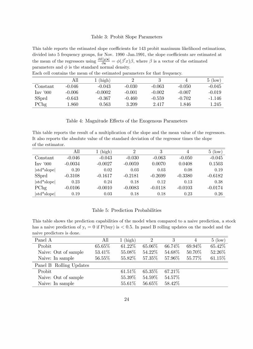
Table 3: Probit Slope Parameters
This table reports the estimated slope coe¢ cients for 143 probit maximum likelihood estimations,divided into 5 frequency groups, for Nov. 1990 -Jan.1991, the slope coe¢ cients are estimated at
the mean of the regressors using @E[yjx]@x
= �(�0x)�, where � is a vector of the estimatedparameters and � is the standard normal density.Each cell contains the mean of the estimated parameters for that frequency.
All 1 (high) 2 3 4 5 (low)Constant -0.046 -0.043 -0.030 -0.063 -0.050 -0.045Inv �000 -0.006 -0.0002 -0.001 -0.002 -0.007 -0.019SSprd -0.643 -0.367 -0.460 -0.559 -0.702 -1.146PChg 1.860 0.563 3.209 2.417 1.846 1.245
Table 4: Magnitude E¤ects of the Exogenous Parameters
This table reports the result of a multiplication of the slope and the mean value of the regressors.It also reports the absolute value of the standard deviation of the regressor times the slopeof the estimator.
All 1 (high) 2 3 4 5 (low)Constant -0.046 -0.043 -0.030 -0.063 -0.050 -0.045Inv �000 -0.0034 -0.0027 -0.0059 0.0070 0.0408 0.1503jstd*slopej 0.20 0.02 0.03 0.03 0.08 0.19SSprd -0.3108 -0.1617 -0.2181 -0.2699 -0.3380 -0.6182jstd*slopej 0.23 0.24 0.18 0.12 0.13 0.38PChg -0.0106 -0.0010 -0.0083 -0.0118 -0.0103 -0.0174jstd*slopej 0.19 0.03 0.18 0.18 0.23 0.26
Table 5: Prediction Probabilities
This table shows the prediction capabilities of the model when compared to a naive prediction, a stockhas a naive prediction of yi = 0 if P(buy) is < 0:5: In panel B rolling updates on the model and thenaive predictors is done.
Panel A All 1 (high) 2 3 4 5 (low)Probit 65.65% 61.22% 65.06% 66.74% 69.94% 65.42%Naive: Out of sample 53.41% 55.08% 54.22% 54.68% 50.70% 52.26%Naive: In sample 56.55% 55.82% 57.35% 57.96% 55.77% 61.15%
Panel B Rolling UpdatesProbit 61.51% 65.35% 67.21%Naive: Out of sample 55.39% 54.59% 54.57%Naive: In sample 55.61% 56.65% 58.42%
24

Table 6: Trades of the Specialist
This table presents the average number of trades in each category and below the percentage in eachcategory. Trades are speci�ed as liquidity providing trades if the specialist is a buyer to a sellerinitiated trade and vice versa. A trade is buyer (seller) initiated if the trade price is above (below)the prevailing midpoint of the quotes. Trades at the midpoint are speci�ed as liquidity trades.
All 1 (high) 2 3 4 5 (low)Total 1563 5379 1350 584 293 116Initiated Trades 446 1629 339 140 69 27
29% 30% 25% 24% 23% 23%Liquidity Trades 1117 3751 1011 444 224 89
71% 70% 75% 76% 77% 77%
Table 7: Trades Initiated
All 1 (high) 2 3 4 5 (low)Total 446 1629 339 140 69 27Buy at Low/ Sell at High 379 1447 258 103 44 18
85% 89% 76% 74% 64% 66%Other 67 182 81 37 25 9
15% 11% 24% 26% 36% 34%
Table 8: Pro�ts for Trading Strategy Cents/Dollar
This table presents the average pro�ts from trading strategies for each trading frequency.Each number represents a simple mean of the variables for each trading frequency. If theliquidity trades pro�ts are corrected for the bid/ask bounce the di¤erence becomeseven more pronounced.
All 1 (high) 2 3 4Total -0.096 -0.079 -0.050 0.059 -0.322Initiated Trades 0.112 0.064 -0.030 0.060 0.364Liquidity Trades -0.200 -0.134 -0.075 -0.018 -0.588
25
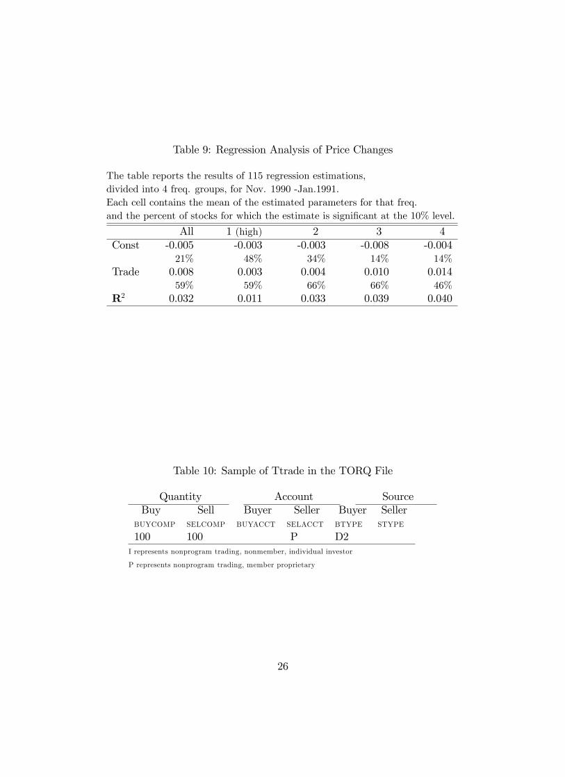
Table 9: Regression Analysis of Price Changes
The table reports the results of 115 regression estimations,divided into 4 freq. groups, for Nov. 1990 -Jan.1991.Each cell contains the mean of the estimated parameters for that freq.and the percent of stocks for which the estimate is signi�cant at the 10% level.
All 1 (high) 2 3 4Const -0.005 -0.003 -0.003 -0.008 -0.004
21% 48% 34% 14% 14%Trade 0.008 0.003 0.004 0.010 0.014
59% 59% 66% 66% 46%R2 0.032 0.011 0.033 0.039 0.040
Table 10: Sample of Ttrade in the TORQ File
Quantity Account SourceBuy Sell Buyer Seller Buyer Seller
BUYCOMP SELCOMP BUYACCT SELACCT BTYPE STYPE
100 100 P D2I represents nonprogram trading, nonmember, individual investor
P represents nonprogram trading, member proprietary
26
Top Related