


Languages
Pages
Legal


An Analysis of Consumer Debt Restructuring Policies∗
Nuno Clara† Joao F. Cocco‡
March 2016
Abstract
We solve a quantitative dynamic model of borrower behavior, whose income is subject
to individual specific and aggregate shocks. Lenders provide loans competitively. Reces-
sions are characterized by lower expected earnings growth and a higher likelihood of a
large drop in earnings. The model generates procyclical credit demand and countercycli-
cal default. We analyze alternative debt restructuring policies aimed at reducing default
during recessions: (i) interest rate reduction; (ii) maturity extension; and (iii) refinancing.
Outcomes are best for the maturity extension policy that allows borrowers to temporarily
make interest-only payments on the loan. Not all borrowers exercise the option. The
maturity extension policy leads to lower default rates, higher consumer welfare, and a
smaller drop in consumption during recessions, without significantly increasing cash-flow
risk for lenders.
∗We would like to thank Francisco Gomes, Ralph Koijen, Henri Servaes and seminar participants at Erasmus
University and London Business School for comments.†Department of Finance, London Business School.‡Department of Finance, London Business School, CEPR and CFS.
1 Introduction
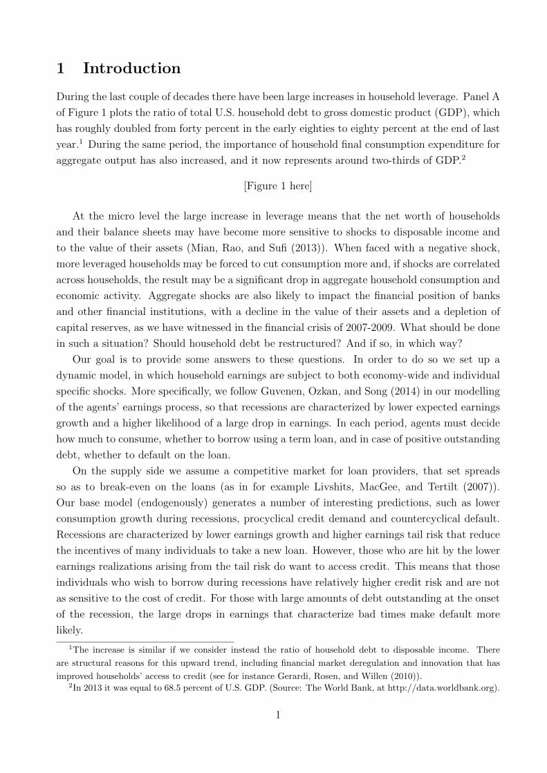
During the last couple of decades there have been large increases in household leverage. Panel A
of Figure 1 plots the ratio of total U.S. household debt to gross domestic product (GDP), which
has roughly doubled from forty percent in the early eighties to eighty percent at the end of last
year.1 During the same period, the importance of household final consumption expenditure for
aggregate output has also increased, and it now represents around two-thirds of GDP.2
[Figure 1 here]
At the micro level the large increase in leverage means that the net worth of households
and their balance sheets may have become more sensitive to shocks to disposable income and
to the value of their assets (Mian, Rao, and Sufi (2013)). When faced with a negative shock,
more leveraged households may be forced to cut consumption more and, if shocks are correlated
across households, the result may be a significant drop in aggregate household consumption and
economic activity. Aggregate shocks are also likely to impact the financial position of banks
and other financial institutions, with a decline in the value of their assets and a depletion of
capital reserves, as we have witnessed in the financial crisis of 2007-2009. What should be done
in such a situation? Should household debt be restructured? And if so, in which way?
Our goal is to provide some answers to these questions. In order to do so we set up a
dynamic model, in which household earnings are subject to both economy-wide and individual
specific shocks. More specifically, we follow Guvenen, Ozkan, and Song (2014) in our modelling
of the agents’ earnings process, so that recessions are characterized by lower expected earnings
growth and a higher likelihood of a large drop in earnings. In each period, agents must decide
how much to consume, whether to borrow using a term loan, and in case of positive outstanding
debt, whether to default on the loan.
On the supply side we assume a competitive market for loan providers, that set spreads
so as to break-even on the loans (as in for example Livshits, MacGee, and Tertilt (2007)).
Our base model (endogenously) generates a number of interesting predictions, such as lower
consumption growth during recessions, procyclical credit demand and countercyclical default.
Recessions are characterized by lower earnings growth and higher earnings tail risk that reduce
the incentives of many individuals to take a new loan. However, those who are hit by the lower
earnings realizations arising from the tail risk do want to access credit. This means that those
individuals who wish to borrow during recessions have relatively higher credit risk and are not
as sensitive to the cost of credit. For those with large amounts of debt outstanding at the onset
of the recession, the large drops in earnings that characterize bad times make default more
likely.
1The increase is similar if we consider instead the ratio of household debt to disposable income. There
are structural reasons for this upward trend, including financial market deregulation and innovation that has
improved households’ access to credit (see for instance Gerardi, Rosen, and Willen (2010)).2In 2013 it was equal to 68.5 percent of U.S. GDP. (Source: The World Bank, at http://data.worldbank.org).
1

It is in the context of this model that we quantitatively evaluate the effects of alternative
consumer debt restructuring policies, that involve some form of concession given to borrowers
during recessions, either in the form of interest or principal reduction, or in facilitating a loan
restructuring. More specifically, we evaluate the following policies: (i) interest rate reduction;
(ii) loan maturity extension, i.e. temporarily allow for interest-only payments on the term
loan, with a corresponding increase in its maturity; and (iii) facilitate loan refinancing during
recessions, i.e. allowing borrowers to prepay the existing loan and to take out a new one.
Our motivation for studying the effects of debt restructuring during recessions is two fold.
First, from an aggregate point of view, leverage and defaults pose particular challenges during
bad times (Kiyotaki and Moore (1997)). They may lead to a downward economic spiral, the
severity of which may be reduced by the debt restructuring policies that we study. Second,
recessions are characterized by lower earnings growth and higher risk, but these aggregate events
are far beyond the control of individual borrowers, which should help to mitigate moral hazard
concerns.3
Another important aspect of our analysis is that we allow all borrowers, regardless of their
savings or income, to take advantage of the restructuring policies if they wish to do so. In
the context of our model with perfect information it would be straightforward to study more
complex restructuring policies, for example that depend on savings. We abstract from this
since implementing these more complex policies in practice may be difficult, as borrowers are
likely to have private information that they may not have an incentive to disclose. Furthermore,
a policy that is made available to all has the additional advantage of being less likely to be
perceived as a bail out of a specific group of individuals. For government sponsored/subsidized
restructuring programs this may be an important consideration, and it may facilitate their
political implementation.
We evaluate the restructuring policies along several dimensions, including their impact on
borrower welfare, defaults, consumption, and on the properties of lenders’ cash-flows. Although
there are trade-offs among the policies, the one that leads to better outcomes is loan maturity
extension. Compared to the base model without debt restructuring, it generates lower uncon-
ditional default rates, lower default rates and a smaller drop in consumption in recessions, and
an improvement in borrower welfare (measured in utility terms, from an ex-ante point of view).
From the lenders perspective, the losses that arise from the postponing of loan principal repay-
ments are offset by the drop in default rates and by the additional interest payments received.
It is also important that not all borrowers decide to exercise the option to extend loan matu-
rity. The lower earnings growth and higher earnings risk that characterize recessions, and the
uncertainty regarding how long the recession will take, lead better off precautionary borrowers
to keep on making the scheduled loan repayments and in this way reduce their leverage. This
3Even though the events that trigger the possibility of restructuring are not the result of borrowers’ actions,
the policies that we study are not immune to moral hazard. As our model results will show, the expectation of
debt restructuring in bad times affects agents’ consumption and borrowing behaviour also in good times.
2
mitigates the impact of the policy on lender cash-flows.
The policy of allowing for a reduction in the loan interest rate in bad times is too costly,
since all borrowers want to take advantage of it.4 It implies that the loan interest rate must
increase sufficiently in good times to compensate lenders for the significantly lower cash-flows
that they will receive in recessions. This reduces the benefits of the policy. On the other hand,
not all borrowers decide to refinance their loans in recessions. Only those who are worse off do
so. This helps to reduce default rates in recessions. However, the increase in debt outstanding
for the refinanced loans means that lender losses on those for which there is default are on
average higher. Lenders need to be compensated for this up-front, which reduces the benefits
of the policy. But the main disadvantage of this policy is its impact on lender cash-flows: they
become significantly more volatile and there is a large number of periods in which lenders need
to have significant amounts of capital to extend loans.
Our paper is related to a large literature on debt and default, and their implications for both
the macroeconomy and asset prices. Seminal papers include Alvarez and Jermann (2000), Fay,
Hurst, and White (2002), and Chatterjee, Corbae, Nakajima, and Rios-Rull (2007). Athreya
(2005) and Livshits (2014) provide surveys of the literature on consumer credit and default. Our
paper is also related to several others that study default in the context of the recent financial
crisis (for example Corbae and Quintin (2015), Adelino, Gerardi, and Willen (2013)). Adelino,
Gerardi, and Willen (2013) is particularly relevant since they address the question of why more
lenders chose not to renegotiate home mortgages. They do not find evidence to support the
notion that renegotiation was hampered by the fact that loans had previously been securitized.
Instead they develop a model that points towards the roles of redefault and self-cure risk in
reducing the benefits of renegotiation for investors. In our model there is also redefault and
self-cure, but we show that the quantitative outcomes depend on the type of restructuring.
Some recent papers have studied the household deleveraging process that takes place during
bad times and its aggregate economic implications (see for instance the important contribution
of Guerrieri and Lorenzoni (2009)). Due to the characteristics of the earnings process, some of
the agents in our model want to (endogenously) deleverage in bad times. And we show that
in order for lenders to be able to break-even in recessions, they may need to restrict access to
credit to the riskiest borrowers. In this way our paper also contributes to the understanding
of the deleveraging process. But its main contribution is to model and quantitatively evaluate
alternative forms of debt restructuring. In order to be able to do so we simplify along certain
dimensions that have been the focus of the above literature (for example we do not solve en-
dogenously for the equilibrium risk-free rate). In addition, we consider a setting with perfect
information and focus on the quantitative implications of the different restructuring policies.
Therefore our approach is very different from the theoretical model of Kovrijnykh and Livshits
(2013) where debt restructuring arises with a positive probability in an optimal screening mech-
anism that deals with an adverse selection friction (the lender cannot observe the cost of default
4The same would be true for a policy that allows for a loan principal reduction.
3
of the borrower).
Our paper is structured as follows. Section 2 describes the model, which we parameterize
in section 3. Section 4 is the main results section. Section 5 extends the main model by
introducing the possibility of credit rationing. The final section concludes.
2 The Model
The demand for credit comes from agents who in each period decide how much to consume,
borrow, and whether to default on existing debt. Lenders provide loans at a rate such that on
average they break-even. In our base model there is no option to restructure the debt. This
base model provides a benchmark to which we compare the effects of alternative restructuring
policies. In this section we describe in detail the several features of the model. Even though we
solve endogenously for the loan premium, our model is in several dimensions partial equilibrium.
This allows us to model in more detail the different restructuring policies.
2.1 Aggregate state
In each period the economy may either be in an expansion or in a recession. An exogenous
transition probability matrix governs the evolution between these states. We define the indicator
function Icyclet to be equal to one if the economy is in an expansion in period t, and zero
otherwise. The demand for credit comes from consumers who are endowed with stochastic
earnings. The state of the economy affects the expected earnings growth and risk.
Risk-free interest rates are also exogenously given, but stochastic. Let r1t denote the
expected log gross real return on a risk-free (of default) one-period bond, so that r1t = log(1 +
R1t). We assume that it follows an AR(1) process:
r1t = µr(1− φr) + φrr1,t−1 + ωt, (1)
where ωt is a normally distributed white noise shock with mean zero and variance σ2ω. We let
innovations to short-term interest rates be correlated with the business cycle variable.
2.2 Agents preferences and earnings
In each period a new set of consumers/households enters our economy and remains in it for T
periods. We model the consumption and debt choices of these agents. Let ti denote the period
in which the agent indexed by i enters the economy. We assume that his/her preferences are
time separable and exhibit constant relative risk aversion:
max Eti
ti+T∑t=ti
βt−tii
C1−γiit
1− γi+ βTi bi
W 1−γii,ti+T+1
1− γi, (2)
4
where βi is the time discount factor, Cit is consumption, and γi is the coefficient of relative risk
aversion. The agent derives utility from both consumption and terminal real wealth, Wi,ti+T+1,
which can be interpreted as the remaining lifetime utility from reaching age T + 1 with wealth
Wi,ti+T+1 or as the utility derived from a bequest. The parameter bi measures the relative
importance of the utility derived from terminal wealth. Individuals are heterogeneous and
our notation uses the subscript i to take this into account. It is worth noting that the above
preferences give rise to a precautionary savings motive, with relative prudence equal to γi + 1.
Each individual that enters the economy is endowed with a stream of stochastic earnings.
There is considerable evidence that the nature of the income risk faced by households varies
over the business cycle. Several papers have provided evidence for and modeled countercyclical
income risk, either in the form of countercyclical variances (among these are Constantinides
and Duffie (1996), Krusell and Smith (1997), Storesletten, Telmer, and Yaron (2007)) or of
countercyclical left-skewness of shocks (Mankiw (1986), Kocherlakota and Pistaferri (2009),
Chen, Michaux, and Roussanov (2013)).
More recently, Guvenen, Ozkan, and Song (2014) have used a large dataset from the U.S.
Social Security Administration to provide evidence for countercyclical left-skewness of earnings
shocks. In recessions large increases in earnings become less likely and large drops become
much more likely. We use their earnings process specification in our model. Let Yit denote the
stream of non-tradable stochastic real earnings of individual i. As usual, we use a lower case
letter to denote the natural log of the variable, so that yit ≡ log(Yit). Log real earnings is equal
to the sum of a transitory (εit) and a persistent (zit) components. Innovations to the persistent
component feature a mixture of normals:
yit = zit + εit, (3)
zit = ρzi,t−1 + ηit, (4)
where εit ∼ N (0, σε) and:
ηit =
η1it ∼ N (µ1,Icyclet, σ1), with probability p1
η2it ∼ N (µ2,Icyclet, σ2), with probability 1− p1,
(5)
where recall the subscript Icyclet indicates whether period t is an expansion or a recession. This
setup allows us to capture important deviations of earnings growth from normality, including
negative skewness and excess kurtosis, and business cycle variation in expected earnings growth
through the different means of the normal distributions. The higher probability of a large drop
in earnings in recessions is likely to affect borrowers incentives to default on the loans and the
benefits of debt restructuring.
We model the tax code in the simplest possible way, by considering a linear taxation rule.
Gross labor income and interest earned are taxed at the constant tax rate φ.
5
2.3 Demand for loans and default
The demand for credit comes from consumers. We model a multi-period (installment) loan
with initial maturity τ . In each period agents with no debt outstanding decide whether to
borrow using such loan. They may wish to do so to smooth consumption over the life-cycle
(earnings grow on average over time) and/or in response to a negative earnings shock. Let t′i
denote the period in which agent i has decided to take out the currently outstanding loan, so
that the remaining loan maturity is given by mit = τ − (t − t′i). Furthermore, let the amount
borrowed by individual i at loan initiation be given by Kit. This amount may depend on
borrower characteristics and the aggregate state at the time that the loan is taken out.
We assume that loans are adjustable-rate, with interest rate given by the one-period bond
rate plus a credit risk premium ψit:
Rloanit = R1t + ψit. (6)
The premium on the loan compensates lenders for the risk of default on the loan outstanding
by borrower i at time t. The subscripts i and t allow for the possibility that the premium depends
on borrower characteristics and aggregate variables at the time that the loan was taken out
(and the premium determined). The loan premium remains fixed over the life of the loan.5 The
period t installment due on the loan (Lit) is given by:
Lit = Rloanit Dit + ∆Di,t+1 (7)
where Dit is the principal amount outstanding on the loan at date t and ∆Di,t+1 is the loan
principal repayment due in that period. In order to simplify the solution of the problem, we
follow Campbell and Cocco (2015) in assuming that the loan principal repayments are the same
as the agent would have to make on loan with a fixed rate, equal to the mean rate on a τ -period
bond plus the credit risk premium.6
This simplifies the problem since then the current level of the outstanding debt is not a
state variable: the loan interest rate, the initial amount borrowed, and the remaining maturity
pin down the currently outstanding level of debt (and principal repayments due).
Borrowers choose in each period whether to default on the loan. We assume that loans
are non-recourse, but in case of default borrowers are excluded from credit markets for the
remaining time horizon. In addition, default carries a utility penalty in the period that the
agent defaults equal to λ, which can be interpreted as a social stigma cost (as in for instance
Gross and Souleles (2002) and Guiso, Sapienza, and Zingales (2013)).
5In the parameterization section we will set τ < T , so that the same individual may take out multiple (not
concurrent) loans over the period in which he/she is in our economy.6To model long-term interest rates, we assume that the log expectation hypothesis holds. That is, we
assume that the log yield on a long-term n-period real bond, rnt = log(1 +Rnt), is equal to the expected sum of
successive log yields on one-period real bonds which are rolled over for n periods plus a constant term premium
ξn.
6
In the baseline model we rule out loan prepayment, but later on we will consider this
possibility. More precisely, we will allow for the possibility that borrowers prepay the loan at a
cost equal to a percentage θP of the currently outstanding loan balance (in the baseline model
we set this cost to infinity). In addition, to simplify the model we assume that borrowers are
only allowed to take out one loan at a time.
2.4 Banks
We assume a competitive market for loan providers that set the loan premium so as to on
average break-even. In our model with perfect information each loan premium could depend
on all the state variables of the problem at the time that the loan is initiated, including the
levels of savings, earnings, and so on. But given the large number of state variables this would
make the problem intractable. Therefore, for most of the cases considered we assume that the
loan premium is the same for all borrowers and time periods. Furthermore, we assume that all
agents who have not previously defaulted are able to access credit. In section 5 we relax these
assumptions and allow for the possibility that credit availability and loan premia depend on
the aggregate state of the economy and on borrower variables such as his/her earnings at loan
initiation.
In period t′i in which agent i takes out a new loan, lender cash-flows are given by:
CF lenderit = −Kit (8)
In periods t subsequent to loan origination and prior to loan maturity, i.e. when t > t′i and
t ≤ t′i + τ , and for the case of no previous default lender cash-flows are given by:
CF lenderit = Lit if 1defit = 0 (9)
CF lenderit = 0 if 1defit = 1 (10)
where 1defit is an indicator function that takes a value of one if the consumer defaults in period
t. Lenders do not recover anything in case of default. We calculate the present discounted value
of the above loan cash-flows using both the risk-free interest rate and a risk-adjusted discount
rate that reflects the fact that cash-flow is more valuable in recessions.7
We use these present value calculations, averaged across all loans granted, to endogenously
determine the loan premium so that lenders’ profitability is the same across the different re-
structuring policy scenarios that we study.
7Our model is in several dimensions partial equilibrium so that we cannot endogenously derive a pricing
kernel. However, we use the model to parameterize an exogenously specified pricing kernel. We give further
details below.
7
2.5 Restructuring policies
We model several private sector led restructuring policies.8 These restructuring policies involve
some form of concession given to borrowers during recessions. We focus on recessions since from
an aggregate point of view leverage and defaults pose particular challenges during bad times
(Kiyotaki and Moore (1997)). They may lead to a downward economic spiral, the severity of
which may be reduced by the debt restructuring policies that we study. In addition, recessions
are aggregate events that are far beyond the control of individual borrowers, which should help
to mitigate moral hazard concerns.
In a recession, lenders offer borrowers the choice of whether to restructure or modify the
loan, who in turn choose whether to accept the offer or not. We assume that lenders commit
to making such offer at loan initiation. Alternatively, one can think of the restructuring as
a borrower option that is included in the initial loan agreement. A simplifying assumption
is that we allow all borrowers, regardless of their savings or income to take advantage of the
restructuring policy (if they wish to do so). In the context of our model with perfect information
it would be straightforward to study more complex restructuring policies, for example in which
the offer to modify the loan depends on borrowers’ savings or income. In our baseline model we
do not analyze such policies since implementing them in reality may be difficult: the information
required is not always available to lenders (or the government) and borrowers may not have
an incentive to disclose it. In the recent financial crisis some lenders and policy makers were
reluctant to offer borrowers mortgage modifications due to a concern that even those who were
not at an immediate risk of default would pretend otherwise so as to benefit from the concessions
(Adelino, Gerardi, and Willen (2013)). Our goal is to study the efficacy of restructuring policies
that are simple and have few information requirements.9
The first restructuring policy that we model is the possibility of extending loan maturity
during recessions. Under this alternative, if borrowers decide to take advantage of it, debt
service will temporarily comprise only interest, with principal loan repayments restarting the
following period, and loan maturity extended by a period. For multi-year recessions, borrowers
choose whether to exercise the option to extend maturity in each of the recession years. Lender
cash-flows for the periods in which the loan is restructured are given by:
CF lenderit = DitR
loanit if 1matit = 1 (11)
where 1matit is an indicator function that takes a value one if at time t agent i chooses to extend
the maturity of the loan.
8These are often referred as the main methods of private debt restructuring that do not re-
quire governmental sponsorship. But the restructuring policies that we study could also be govern-
ment supported. See for example the IMF Staff Position Note on Household Debt, available at
https://www.imf.org/external/pubs/ft/spn/2009/spn0915.pdf.9In addition, a policy that is made available to all borrowers has the additional advantage of being less likely to
be perceived as a bail out of a specific group of individuals. For government sponsored/subsidized restructuring
programs this may be an important consideration, that may facilitate their political implementation.
8

The second restructuring policy that we consider is a modification to the loan terms, in the
form of a loan interest rate reduction during recession period t. In recessions borrowers still
need to pay the principal due according to the original repayment schedule, but the interest
payment required is lower so that:
CF lenderit = Dit(R
loanit −∆R) + ∆Di,t+1 if 1rateit = 1 (12)
where ∆R is the interest rate reduction offered. Borrower choice in this case is trivial: all agents
will take-up the offer to modify the loan (the indicator function 1rateit will always be equal to
one when the choice is offered).
The third policy that we model is loan refinancing: borrowers are allowed to take out a new
loan but they must use part of the proceeds to repay the previously outstanding debt. Let 1refitbe an indicator function that takes the value of one if the agent restructures his debt, and zero
otherwise, and tR the period in which the loan is restructured. Lender cash-flow is given by:
CF lenderit = DitR
loanit +Dit −Ki,tR if 1refit = 1 (13)
where the first two terms correspond to the repayment of the pre-existing debt and the last
term the loan taken out in the re-structuring.
2.6 The optimization problem
To more clearly evaluate the effects of the alternative policies that we study, we first solve the
model for a case in which restructuring is not possible. We then analyze each one of the three
restructuring policies at a time.
The timing within a period is as follows. The agent starts period t with wealth Wit and labor
income Yit is realized. Following Deaton (1991) we define cash-on-hand as Xit = Wit + Yit. In
each period the agent decides how much to consume Cit, whether to take out a new loan (if no
loan outstanding nor previous default), and whether or not to default on the loan outstanding
(if any). Agents take loan terms as given. For the scenarios in which restructuring is possible,
an additional choice variable in recessions is whether to restructure the loan.
The state variables are: the time period t, whether the economy is in an expansion or re-
cession (Icyclet ), the real interest rate (R1t), cash-on-hand (Xit), the level of permanent income
(Zit), the initial loan amount (Kit), the remaining loan maturity (mit), and whether the agent
has previously defaulted on his/her debt (Idefit ). Each of the three problems for when restruc-
turing is allowed does not require any additional state variables.10 We setup the consumer
problem recursively and define two distinct value functions: Vit(·) is the value in case of no
10This is because of instead of keeping track of the period when the currently outstanding loan was initiated
we keep track of the number of remaining loan periods. When loan maturity is extended the remaining number
of loan periods is unchanged.
9
previous default and loan repayment in period t and V defit (·) is the value of defaulting in period
t. In case of no previous default the Bellman equation for this problem is given by:
Vit(Xit, Zit, Icyclet , R1t, Kit,mit) = max{U(Cit) + βEt max[Vi,t+1(·), V def
i,t+1(.)]} (14)
where V def denotes the value obtained from defaulting on the debt. It is given by:
V defit (Xit, Zit, I
cyclet , R1t) = max{U(Cit)− λ+ βEtV
defi,t+1(·)} (15)
In case of no previous default the agent maximizes equation (14) subject to the law of
motion for cash-on-hand and the other model restrictions. In case of previous default the agent
maximizes (15) (except that the stigma cost of default is only paid in the period in which
default occurs).
In periods when the agent does not default nor take out a new loan, cash-on-hand evolves
according to (if there is no debt outstanding Lit is equal to zero):
Xi,t+1 = (Xit − Cit − Lit)(1 + (1− φ)R1t) + (1− φ)Yi,t+1 if 1defit = 0 (16)
In periods in which the agent takes out a new loan:
Xi,t+1 = (Xit − Cit − Lit +Kit)(1 + (1− φ)R1t) + (1− φ)Yi,t+1 (17)
where Lit denotes the last payment on any previously outstanding loan. In case of default the
law of motion for cash-on-hand is simply given by:
Xi,t+1 = (Xit − Cit)(1 + (1− φ)R1t) + (1− φ)Yi,t+1 if 1defit = 1 (18)
For the case in which there is the possibility of extending loan maturity the equation describing
the evolution of cash-on-hand is:
Xi,t+1 = (Xit − Cit −DitRLoanit )(1 + (1− φ)R1t) + (1− φ)Yi,t+1 if 1matit = 1 (19)
And for the refinancing policy, in periods when the agent refinances the loan:
Xi,t+1 = (Xit−Cit−Dit(1+RLoanit )+Ki,tR)(1+(1−φ)R1t)+(1−φ)Yi,t+1 if 1refit = 1 (20)
The problem of the agent cannot be solved analytically. We solve it numerically via backward
induction, using grid search, non-linear value function interpolation and gaussian quadrature
methods. We give details on the numerical solution technique in Appendix A. The agent solves
his/her problem given the loan premium.
In each period t a new set of agents enters the economy and they remain in it for T periods.
They take the loan premium that they are offered as given. Banks provide loans to these
agents and set the loan premium so as to on average break-even across all loans granted. In the
baseline version of the model we simplify by assuming a similar loan premium for all agents and
10
time periods, so that ψit = ψ. However, when we compare across restructuring policies we solve
endogenously for the loan premium so that lenders’ profitability is the same across the different
scenarios. Furthermore, in section 5 we allow for the possibility that the loan premium varies
over time with the aggregate state of the economy and that banks screen borrowers based on
their earnings.
It is important to note that even though we solve endogenously for loan premia our model
is not a full general equilibrium one: we do not clear the market for consumer loans nor do we
solve endogenously for the risk-free rate. By simplifying along these dimensions we are able to
model with much more realism the different restructuring policies.
3 Parameterization
We use a combination of approaches to parameterize the model, including data, parameter
values from the literature, and calibration. Each period corresponds to one year.
3.1 Business cycle, interest rates and earnings
To parameterize the annual transition probability matrix for expansions/recessions we use the
NBER Business Cycle Dates, from 1855 to 2013. The latter data are quarterly, so we first
classify each calendar year as a recession year if for three or four quarters during that year the
economy was in a recession. According to this classification, the proportion of recession years is
22%, so that the economy is in a recession on average for one year in every five. The transition
probabilities between expansion/recession are reported in Panel A of Table 1.
[Table 1 here]
We choose the earnings process parameters to match the cyclicality of earnings documented
by Guvenen, Ozkan, and Song (2014). We use their “persistent-plus-transitory” specification
and report their estimated parameters in Panel B of Table 1. Recall that their error structure
features a mixture of two normals, whose moments are denoted by (1) and (2) in the table. As
Guvenen, Ozkan, and Song (2014) explain, the two normals can be economically interpreted as
between-job (1) and with-in jobs (2) earning changes, or as idiosyncratic and aggregate shocks.
In any given year, with probability p1, the agent changes job and his/her earnings shocks have
a large standard deviation, equal to 0.325 (determined mainly by idiosyncratic factors). With
probability 1 − p1 the agent does not change jobs, earnings growth is mainly determined by
aggregate factors, and it has low dispersion. The means of the normal distributions are such
that expected earnings growth is considerable lower in recessions than in expansions.
11

3.2 Preferences
In our benchmark parameterization we set the coefficient of relative risk aversion (γ) equal to
2 and the subjective discount factor (β) equal to 0.80. Given the large consumer loan interest
rate observed in the data we need to use a sufficiently low value for β to provide the agent with
the appropriate incentives to take on consumer debt. In order to reduce further the agent’s
incentives to save, we set the bequest parameter to zero. We interpret the agents in the model
as being at an early stage of the life-cycle and not yet concerned with saving for retirement.
Accordingly, we set T equal to twenty. The benchmark preference parameters are summarized
in Panel C of Table 1.
3.3 Interest rates and loan parameters
We follow Campbell and Cocco (2015) in the parameterization of the log real interest rate. We
set the average log real interest rate to 1.2%, the persistence coefficient to 0.825, the standard
deviation of shocks to 1.8%, and the term premium to 0.5% (Panel D of Table 1). We have
used the data to calculate mean real interest rates in recession and expansion years. The mean
real interest rate in recessions (expansions) is 2.44% (1.54%). The difference is not statistically
significant, so that in our baseline parameterization the level of real interest rates does not
depend on whether the economy is in an expansion or recession.11
There are two main types of household debt: consumer debt (credit card debt, consumer
loans) and mortgage debt. In terms of their relative importance, consumer debt constitutes
around one-third and mortgage debt around two-thirds of the total outstanding household
debt.12 These two types of debt differ along several important dimensions. Consumer debt is
predominantly unsecured (car loans are an exception) and mortgage debt is secured. Accord-
ingly, house values that tend to fluctuate with aggregate economic conditions are an important
determinant of the value of mortgage debt. Consumer debt is more prevalent among lower
income households whereas mortgage debt is more prevalent among higher income households.
In the U.S. consumer debt tends to be predominantly (but not exclusively) adjustable-rate
whereas long-term fixed rate are the predominant form of mortgage contracts. The loans in our
model are most similar to unsecured consumer loans, so that we use data on this type of debt
to parameterize them.
In Figure 2 we plot the evolution over time of consumer loan spreads (both credit card
debt and personal loans spreads). Spreads are on average higher for credit card debt than
for personal loans. Furthermore, spreads tend to fluctuate over time, mainly as a result of
fluctuations in interest rates. Spreads tend to increase in recessions, and to remain high for
11It would be straightforward to relax this assumption and study the quantitative effects of a reduction in
interest rates in bad times.12The weight of both consumer debt and mortgage debt on disposable income has significantly increased over
time: mortgage debt and consumer debt represented 40% and 15% of disposable income in the early eighties
compared to roughly 70% and 25% at the end of 2014, respectively.
12
a number of years after the end of the recession, so that when we compare the average level
of the spread between recessions and expansions their difference is not statistically significant
(first two rows of Table 2).
[Figure 2 here]
In several of the experiments that we carry out we solve endogenously for loan spreads.
However, in order to do so from first principles we would need estimates of the costs and
normal profits of loan providers, which we do not have. To overcome this difficulty, we first
solve our model setting the loan premium equal to the average value observed in the data
of (roughly) 8% (for personal loans, which better resemble the type of loan we model). We
then calculate the profits of loan providers, which we take to be the normal profits. In the
experiments that we carry out we solve for the loan premium that generates this same level of
average profits.13
[Table 2 here]
We use data from the Survey of Consumer Finances to parameterize the loan amount (Kit).
In these data the average value of consumer installment loans outstanding (excluding education
and auto loans) per household has increased from 5.8 thousand dollars in 1989 to 15.9 thousand
dollars in 2013 (conditional on the household holding positive debt). Dividing the latter value by
the average number of adult household members of 1.6 gives us an average amount outstanding
of 9.93 thousand dollars. With this in mind, we set the loan amount in our model to ten
thousand dollars.14
A final loan related parameter that we need to calibrate is the utility penalty in case of
default (λ). We choose its value so that our baseline model (roughly) matches the average
default rates observed in the data. There are several measures of default that we could use,
including delinquency rates, charge-off rates, and personal bankruptcy filings. For the former
two we have data by loan type, that we plot in Figure 3, Panels A and B, respectively. For
consumer loans delinquency rates are on average higher than charge-off rates, equal to 3.5% and
2.5% respectively. Some of the loans that are past due are eventually repaid, so that lenders
do not incur a loss.
A third default measure is bankruptcy filings. It is defined as the proportion of households
that file for bankruptcy in a given year. As Panel C of figure 3 shows there has been a large
increase in filings over time from an annual rate of less than half a percent in the early eighties
13In the baseline model we set the premium equal to 8% for both recessions and expansions, and focus on
unconditional profits, but in section 5 we relax this assumption. The fact that the average loan premium is
not statistically different across expansions/recessions does not mean that lenders do not differentiate between
loans granted at different stages of the business cycle, since the riskiness of the loans granted may be different.
We will come back to this, important point, later in the paper.14In a future version of the paper we plan to expand the set of loan choices available to agents.
13

to values over one percent in the more recent years.15 With these several data sources in mind,
in our baseline parameterization we target an average default rate of 2%, somewhat higher than
bankruptcy filings but lower than annual charge-off rates on consumer loans.
[Figure 3 here]
It is important to note that we set λ to be the same in expansions and recessions. Therefore
any model generated differences in default rates between recessions and expansions are due to
differences in earnings characteristics and the choices of the agents in the model. In the data
we observe delinquency and charge-off rates that are significantly higher in recessions than in
expansions (the last column of Table 2 reports the t-statistic for a test for the equality of means
for recessions and expansions). In the last two rows of Table 2 we report percentage changes in
total U.S. consumer debt outstanding (also as a ratio of household disposable income). The last
row shows that consumer debt as a ratio of disposable income is procyclical, which contrasts
with the countercyclical nature of default rates. In our baseline calibration we do not allow
agents to prepay their loans (the prepayment cost is set equal to infinity). The loan parameters
are summarized in Panel E of Table 1.
3.4 Risk adjusted discount factors
In order to be able to compare across restructuring policies we need to calculate the present
discounted value of the lenders’ cash-flows. We compute such present values using both risk-
free interest rates and risk-adjusted discount rates. The former do not take into account that
cash-flows received during recessions tend to be more valuable than cash-flows received during
good times. In order to somehow take this into account, similar to the approach of Campbell
and Cocco (2015), we use our model to derive risk-adjusted discount rates.
We proceed in steps. First, we solve the model for agents with a coefficient of relative risk
aversion equal to 0.5, a rate of time preference β equal to 0.99 and a bequest motive intensity
b equal to one. Such agents may be interpreted as the long-horizon version of the more myopic
agents in our model of consumer debt (agents with β equal to 0.80 and a b equal to zero).16
Second, we use our model results for such agents to calculate expected consumption growth
rates for different states of the world (recession/expansion and low/high risk-free interest rates),
averaged across all agents. Finally, we use these consumption growth rates to derive a pricing
kernel for each state of the world. The implicit assumption is that the marginal utility of
a representative long-horizon agent is the relevant metric for pricing cash-flows received in
15The annual average over the last decade is 1.05%. The large drop in 2006 follows the passage of the
Bankruptcy Abuse Prevention and Consumer Protection Act of 2005, which was effective October 2005.
Bankruptcy rates have since then increased.16The reason why we set the coefficient of relative version to a lower value of 0.5 is that otherwise the
calculations described below predict an unrealistically high risk-free rate.
14
different states of the world. Table 3 reports the values of the discount rates.17 We will perform
sensitivity analysis on these.
[Table 3 here]
3.5 Simulated data
We use the stochastic processes for the exogenous variables and the policy functions for the
agent choices to generate simulated data. We first generate four hundred different paths for
the aggregate variables (recession/expansion and the level of interest rates) over a forty year
period. In each of these periods a new set of five hundred agents enters the economy, for whom
we generate earnings and simulate choices over their twenty year horizon (after which they
drop out from our simulated data). Finally, we discard all the data corresponding to the first
twenty years of the aggregate variables. This ensures that in each period a new set of agents
enters our economy at the same time that a set of agents drops out from our sample. Thus
the total number of observations is four million (four hundred aggregate paths × five hundred
individuals per aggregate path/period × twenty periods). We generate simulated data for the
different experiments that we carry out, but the realizations for the random variables are the
same throughout. The results that we discuss in the next section are based on these simulated
data.
4 Results
We first describe the baseline model results in which there is no debt restructuring. We then
evaluate the impact of the different restructuring policies.
4.1 Baseline results
The first three rows of Table 4 report the first three moments of log earnings growth. The
table reports both unconditional moments and moments conditional on whether the economy
is in a recession or in an expansion. Earnings moments result directly from our specification
and parameterization of the earnings process and are the same for all the experiments that we
carry out. On average log earnings grow at an annual rate of 2.7%, but there are significant
differences between recessions and expansions, with average annual growth rates of −0.8% and
3.7%, respectively. The standard deviation of log earnings growth is fairly high, but similar for
17Since the discount rates for future cash-flows are higher in recessions than in expansions, cash-flows received
during recessions are more valuable. It is important to note that our model is not a general equilibrium one,
and that we do not clear the market for consumer loans. We are simply using the consumption choices of the
long-horizon agents to specify a pricing kernel that takes into account differences in marginal utility across states
of the world.
15
recessions and expansions. Recessions are riskier because of the higher probability of a large
drop in earnings, as reflected in left-skewness of the earnings growth distribution.
[Table 4 here]
To better understand the effects of debt we briefly discuss the results from a model where
borrowing is not allowed. Panel B of Table 4 reports measures for the first three moments of log
consumption growth, based on agents’ optimal choices, for such a model. As expected, earnings
characteristics are reflected on consumption choices and properties. Average log consumption
growth is negative during recessions, so that agents cutback on consumption during bad times.
They do so because they expect lower earnings growth, but also because earnings risk is higher
and they have a precautionary savings motive. These two channels lead to a drop in average
log consumption growth during recessions that is slightly higher (in absolute value) than the
drop in average log earnings growth. In spite of this, agents are able to achieve some smoothing
of idiosyncratic earnings shocks: the standard deviation of log consumption growth is 0.29
compared to a standard deviation of log earnings growth equal to 0.35. The final row of
Panel B reports the average savings generated from the model. They are equal to roughly one
thousand dollars, reflecting the fact that agents in our model do not have much of an incentive
to save. Thus one should not interpret our buffer-stock model of saving and borrowing behavior
as being one of a representative consumer.
In Panel C we report results for the baseline model with consumer debt. Average annual
log consumer growth is considerably smaller than in the model without debt, 2.2% compared
to 3.1%, respectively. Therefore, debt allows agents to achieve better lifetime consumption
smoothing. The difference in consumption growth rates between recessions and expansions is
larger, though. When the economy is hit by a recession, those agents who have debt outstand-
ing are forced to cut consumption by more, as part of their earnings are used to meet debt
repayments. The quantitative effects are significant: a drop in consumption of 2.7% during
recessions, compared to a drop of 1.3% in the model without debt. The larger drop in con-
sumption growth that takes place during recessions helps to explain why the model with debt
generates larger skewness in log consumption growth than the model without debt. Debt is
beneficial for the agents in our model: the welfare gain of agents from having access to credit,
calculated in the form of an equivalent consumption variation, is 1.93% of annual consumption.
The last two rows of Table 4 report lenders’ average net present values (at loan initiation)
of loan cash-flows (using either the risk-free interest rate or the risk-adjusted discount rate to
discount future cash-flows). Their unconditional values are equal to 1.476 and 0.680 thousand
dollars, respectively. We interpret the latter value as being the one that covers the costs and
normal profits of loan providers. In the different restructuring experiments that we carry out
we solve for the loan premium that matches this value.
Table 4 also reports average net present values at loan initiation for loans initiated in
recessions and in expansions. There are significant differences across the cycle, particularly
16
when one considers the risk-adjusted calculations. Loans granted in recessions are on average
riskier and achieve significantly lower profitability, suggesting that lenders should increase loan
premia during bad times. However, in the data we did not find statistically significant differences
in average premia in recessions and expansions, so that in this section we set the loan premium
to be the same across these periods.18
To better understand the model generated business cycle debt dynamics, Panel A of Table
5 reports the probability that agents decide to take out a new loan (conditional on them
being allowed to do so, i.e. not having a loan outstanding nor having previously defaulted).
On average in each period one in four agents decide to take a new loan. High interest rates
reduce the demand for debt: the probability that a new loan is initiated when interest rates
are high is 24% compared to 26% when interest rates are low. The differences over the cycle
are quantitatively more significant: the probability that a new loan is initiated in a recession
is 18% compared to 27% in an expansion. Recessions are characterized by lower expected
earnings growth and higher earnings risk, both of which reduce agents’ incentives to borrow.
The lower incentives to borrow in bad times are reflected in the policy functions: for given
levels of permanent income and interest rates, the cash-on-hand threshold below which agents
do not take on any debt is higher in recessions than in expansions.
[Table 5 here]
There is however an additional channel: recessions are characterized by a higher probability
of a large drop in earnings. Those agents who are hit by the drop do want to borrow. This
is visible in Panels B and C of Table 5 where we compare average earnings for those agents
who decide to take out a new loan and for those who decide not to borrow. As expected, those
agents with lower earnings and savings are the ones who decide to take out a loan. Interestingly,
the differences in earnings relative to those who decide not to borrow are larger in recessions
than in expansions. The ratio of average earnings between those who do not take out a new
loan and those who do so is 1.7 (1.5) in recessions (expansions). Thus, our model generates
fairly rich business cycle debt dynamics: recessions are characterized by a lower overall demand
for credit, but also by a shift in the composition of borrowers towards relatively high risk (low
earnings) agents.
The final Panel of Table 5 reports the probability that agents take a new loan in the period
when the previous loan matures.19 These probabilities are considerably higher than those in
Panel A that are not conditional on individuals/periods in which a previous loan matures.
This reflects the fact that there is persistence in earnings and in the set of agents who find it
beneficial to borrow.
While the demand for credit in our model is procyclical, default is countercyclical. In Panel
A of Table 6 we report annual default probabilities. Average annual default rates are as high as
18In section 5 we relax this assumption and allow for the possibility that the loan premium is higher for loans
granted in recessions.19Recall that for tractability we have assumed that individuals may only have one loan outstanding at a time.
17

2.8% in recessions, compared to 1.6% in expansions. The average unconditional annual default
rate is 1.8% which is the value targeted by our calibration of the utility cost of default λ. Recall
that this cost is the same during good times and bad times, so that the differences in default
rates over the cycle arise from the different earnings characteristics. During recessions more
borrowers are hit by a large drop in their earnings, and the resulting lower cash-on-hand leads
them to default. Default probabilities are higher when interest rates are high than when they
are low, but the quantitative difference is smaller than the difference in default rates between
expansions and recessions.
Panels B and C of Table 6 compare the characteristics of those who decide to default to
those who decide not to do so. On average defaulting agents have lower earnings, they have
recently experienced a large negative earnings shock, and they tend to have higher levels of
outstanding debt.
The default rates reported in Panel A are per period, i.e. based on the proportion of loans
outstanding at the beginning of the period for which there is default in that period. Some of
these loans were initiated in recessions and others in expansions. In the last panel of Table 6
we report per loan default probabilities, conditional on the state of the economy when the loan
was initiated (and not when default occurred). These default probabilities are calculated using
one observation per loan and they are not annualized, thus their larger values. Loans granted in
recessions are considerably riskier than loans granted in expansions. This is because recessions
are persistent and characterized by lower earnings growth and higher earning risk, and because
agents who take out loans in recessions tend to have lower earnings.
[Table 6 here]
As an illustration of the effects at work in our model in Figure 4 we plot simulated cross
sectional means of log earnings and consumption growth, leverage and default for an economy
calibrated to match the 1993-2013 period in terms of the business cycle and interest rate fluctu-
ations. We simulate the optimal decisions for five thousand agents. Recession years correspond
to the shaded areas in the figure. Earnings and consumption growth decline in recessions. Con-
sumption growth also responds to the fluctuations in the real interest rate that we plot in the
second panel. In the third panel we plot two measures of leverage: the ratio of total outstanding
debt to total earnings and the growth rate in total debt outstanding. There is a deleveraging
in the economy during recessions, with a negative growth rate in total debt outstanding (right
scale). The fourth panel in the figure plots default rates: they increase in recessions and when
interest rates go up. The decline in interest rates that took place in the recession year of 2001
helps to explain why the model predicted default rates for this year are not as high as those for
the 2008 recession. The last panel of Figure 4 plots lender cash-flows. They tend to be higher
in periods in which there is deleveraging.
[Figure 4 here]
18

4.2 Restructuring Policies
We now study the effects of allowing for debt restructuring. We evaluate the impact of the
policies on several variables, including consumption, demand for credit, default, agents’ welfare,
and lenders’ cash-flows. To facilitate the comparison we first report results for the same loan
premium as in the baseline model. But we also solve (and report results) for loan premia
endogenously determined so that lenders’ expected profitability is the same as in the baseline
model. We consider the effects of each of the restructuring policies one at a time, but we use
the same realizations for the shocks throughout.
4.2.1 Loan maturity extension
When a recession hits borrowers have the option to extend loan maturity by one period and to
temporarily make only interest payments on the loan. Panel B of Table 7 reports the effects of
this restructuring policy for a constant loan premium of 8%. And to facilitate the comparison
in Panel A we report the previously discussed baseline model results where restructuring is
not allowed. From the comparison of the consumption growth rates we see that the policy
allows agents to better smooth consumption over the life-cycle: the unconditional average log
consumption growth is equal to 2.1% compared to 2.2% in the baseline model. Agents are
also better able to smooth consumption across aggregate states: the average growth rate of
consumption in recessions is now higher and the difference between recessions and expansions
smaller. The fact that debt has now become more attractive is reflected in the higher probability
that agents decide to take out a loan: 26.4% compared to 24.9% in the baseline model.
[Table 7 here]
Even though in economies where restructuring is possible leverage is on average higher,
annual default probabilities are marginally lower. The main difference as far as default is
concerned is the shift that occurs from recessions to expansions. The fewer agents who default
in bad times do so at higher values of outstanding debt: 8.7 compared to 8.4 thousand dollars.
Lenders’ average net present values of loan cash-flows are higher than in the base case (both
when discounted at the riskfree rate and at the risk-adjusted discounted rate). The slightly
higher losses in case of default are more than offset by the fact that on average loans last longer,
with larger amounts of debt outstanding (due to the deferment of principal repayments), and
lenders earn the premium on those loans that do not default. In a competitive market one
might expect loan premia to decrease so that lenders profitability is the same as in the base
model.
In Panel C of Table 7 we report the results for a loan premium calculated so that lenders’
unconditional risk-adjusted net present value of loan cash-flows is the same as in the base
case (0.68 thousand dollars). Since lenders’ cash-flows depend on agents’ choices and the latter
depend on the loan premium, the calculation of the premium that generates the same net present
19
value requires us to solve several iterations of our model to find a fixed point. The loan premium
that yields such fixed point is 7.225%. This lower loan premium contributes to a further
reduction in default probabilities and makes debt even more attractive: the unconditional
probability of a new loan increases to 0.3 and the welfare gain of the option to extend maturity,
calculated as the certainty equivalent consumption stream that makes the individual as well off
as in the case when restructuring is not possible, increases to 0.75%.20
In order to investigate further the decision to restructure, in Table 8 we report the proportion
of borrowers who exercise the option to extend maturity. Not all borrowers decide to extend
maturity: the overall proportion of those who decide to do so is 0.57, it is at its highest level of
0.80 early on, and it declines over the life of the loan, except in the last period when it increases
again (third column of Panel A).21 In the last period, when faced with a recession, a higher
proportion of borrowers take a cautious approach and extend maturity. Of those who do not
extend, 45% do so to take out a new loan and in this way access new funds (Panel B).
Both for the baseline model and for the model with the maturity extension option, the
probabilities of a new loan conditional on the previous one maturing are higher than the un-
conditional probabilities of a new loan, so that there is persistence in the borrowers who decide
to make use of debt to finance consumption. For instance, for the baseline model the probability
of a new loan upon maturity of the previous one is 0.50 (0.41) for an expansion (recession), and
the corresponding unconditional probability is 0.27 (0.18) as reported in the first row of Table
5. The agents with lower earnings are the ones who decide to borrow, and there is persistence
in earnings.
[Table 8 here]
In Panel C we report average earnings for those agents who decide to extend loan maturity.
Before the last period of the loan the agents who do so are those with intermediate earnings.
Those with very low earnings default, those with high earnings repay as planned. In the last
loan period those with lower earnings repay and take out a new loan. The values for average
earnings are 14.4, 20.3 and 38.4 for those who decide to repay and take out a new loan, extend
loan maturity, and repay and not take a out a new loan, respectively (conditional on a recession,
Panel D).
The last panel of Table 8 reports the proportion of agents/periods for which there is a given
loan amount outstanding (for agents who have not previously defaulted). Compared to the
baseline model, the probability mass on larger loan amounts is increased and there is a smaller
20For each scenario, including the benchmark case and the one in which restructuring is allowed, we compute
the certainty equivalent, i.e. the steady consumption stream that makes the agent as well-off in expected utility
terms. The welfare gain is then the percentage of the consumption stream that agents are willing to give up
not to have acess to the option to extend the loan maturity. We perform analogous calculations for the other
restructuring policies.21Due to the possibility of extending maturity, there is no longer a one-to-one mapping between amount
outstanding and loan period.
20
proportion of observations corresponding to agents/periods with zero loan amount outstanding.
Thus there is an increase in leverage in the economy both because agents are more likely to get
a new loan and because restructuring delays principal repayments.
4.2.2 Interest rate reduction
The second restructuring policy that we study is the option to obtain a reduction in the loan
interest rate of one hundred basis points during recessions. Borrowers still make the principal
repayments as scheduled, but the interest due on the outstanding debt is lower.22 All borrowers
(trivially) exercise the option (Panel A of Table 8), so that this policy may also be interpreted
as contingent debt, with lower servicing costs in bad times. These are precisely the times when
expected earnings growth is lower and when there is a higher probability of a large drop in
earnings. Borrowers benefit from debt structured in this way: the welfare gain relative to the
base case is 0.09% (Table 9, Panel B). There is however a less desirable aspect of the policy
which is the fact that ex-post, i.e. when a recession hits, all agents take advantage of it,
regardless of whether there has been a large fall in their earnings. This leads to a reduction in
lenders’ profitability.23
[Table 9 here]
In order for this policy to generate the same (unconditional) risk-adjusted net present value
per loan as the baseline model (of 0.68 thousand dollars per loan), the loan premium must
increase to 8.25% (Table 9, Panel C). This reduces the benefits of the policy for borrowers to
0.04%, a value significantly lower than the one we obtained for the maturity extension policy.
It is possible that other combinations of reduction in loan rate in recessions and higher loan
premium generate higher welfare gains for borrowers and the same profitability for lenders. But
the important shortcoming of this policy that ex-post all borrowers will want to take advantage
of it will still be there. This reduces the efficacy of the policy.
4.2.3 Refinancing
In our last policy experiment we allow agents to refinance their debt. This means that in
recessions they are allowed to take out a new loan even if there is debt outstanding, but they
must also use the proceeds from the new loan to repay any previously outstanding debt. The
22We have experimented with alternative values for the interest reduction. The main shortcoming of this
policy that we discuss below remains.23If it was possible to offer the option to restructure only to those who have lower cash-on-hand and earnings
the drop in lenders’ profitability would be smaller. In reality, it may be difficult for lenders to obtain complete
information on individuals’ savings and earnings. And borrowers may have the incentive to pretend that their
financial situation is worse than it actually is so as to benefit from the interest reduction. Furthermore, the
offering of an interest reduction only to a specific group of individuals may be perceived as a bail out of this
group.
21

results are shown in the last column of Table 8. Not all agents exercise the option to restructure
(Panel A), those with lower earnings do so (Panel C). These are the agents who benefit the
most from any additional funds that they access under the restructuring. There is however
a significant increase in leverage in this economy: the proportion of agents/periods with the
highest loan amount outstanding is 0.21 compared with 0.13 in the baseline model (Panel E).
The effects of the policy on consumption, default and borrower welfare are shown in Table
10. This policy allows for better life-cycle consumption smoothing and better consumption
smoothing across states than both the baseline model and the maturity extension policy, as
it can be seen by the lower average (unconditional) consumption growth rate and the smaller
difference in consumption growth rates across business cycle states.
For a constant loan premium, unconditional default rates are marginally lower than in the
baseline model and there is a significant shift in default from recessions to expansions. The
few agents who default in bad times do so at the highest possible value of outstanding debt
(otherwise the agents would simply refinance). The higher average loan losses in case of default
are a feature of this policy: 8.7 thousand dollars per loan compared to 8.4 thousand dollars per
loan in the baseline model.
[Table 10 here]
In spite of the higher average loan losses in case of default, lenders profitability is higher
than in both the baseline model and the maturity extension policy. The loan premium so that
lenders’ (unconditional) risk-adjusted net present value of cash-flows is equal to the baseline
value of 0.68 thousand dollars per loan is 6.785% (Panel C of Table 10), which is lower than
in the maturity extension policy (recall that it was equal to 7.225%). This lower premium
increases the welfare benefits of the policy for borrowers to 1.17% of annual consumption. The
main shortcoming of this policy is the large downside risk that it imposes on lenders’ cash-flows,
an issue that we now investigate.
4.2.4 Lenders’ cash-flows
If the risk-adjusted discount rates that we have derived fully capture the risks that financial
institutions face, the relevant properties of lender cash-flows are captured in the discounted
cash-flows. But one may reasonably question the extent to which the risk-adjusted discount
rates derived from consumption fully capture such risks, including funding risk, regulatory risks
arising from value at risk constraints, among others.
With this in mind, we use the simulated data to plot in Figure 5 the distribution of lenders’
cash-flows for the baseline model and for the different restructuring policies. Focusing first
on the unconditional distribution for the maturity extension policy, we see that shape of the
distribution is fairly similar to the benchmark model. In fact, under the maturity extension
policy lenders have higher average cash-flows and lower standard deviation of cash-flows. How-
ever, they face more downside risk: the skewness is -0.18 compared to -0.03 in the benchmark.
22
The comparison of the distributions for recessions and expansions helps us to understand why.
Relative to the baseline model, in the maturity extension policy the distribution of per-period
cash-flows in recessions is shifted to the left, as some borrowers exercise their option to postpone
principal repayments.
[Figure 5 here]
These effects are clearly visible in Table 11 where we report summary statistics for the
distributions of lenders’ cash-flows. Panel D reports the proportion of periods in which lenders
have negative cash-flows. The overall proportion for the maturity extension policy is 0.14
compared to 0.20 in the baseline model. The proportions conditional on recession (expansion)
are 0.12 (0.14) compared with 0.02 (0.26) in the baseline.
However, the value for recessions for the maturity extension policy is an order of magnitude
smaller than the value for the refinancing policy scenario: for the latter the proportion of
recession periods with negative cash-flows is as high as 0.73 as existing borrowers exercise the
option to refinance to access cash. As a result, the average per period lender cash-flows are
negative in recessions (Panel A), the only policy for which this happens. The large downside
risk in lenders cashflows for the refinancing policy is clearly visible in the last set of panels
in Figure 5. The overall skewness of lenders’ cash-flows is as high as -0.76. Therefore the
refinancing policy exposes lenders to very large downside cash-flow (and funding) risk which is
an important shortcoming of the policy.24
[Table 11 here]
In light of these results, a natural question to ask is the extent to which the net present
value of lenders’ cash-flows is sensitive to our previous choice of risk-adjusted discount rates.
In Figure 6 we address this question. More precisely, we consider the impact of a reduction
of ∆e in the discount rate in expansions and an increase in the discount rate in recessions of
∆r, calculated so that the overall average discount rate remains unchanged. Panel B plots the
results when we apply different values for the mean-preserving spreads to the previously used
risk-adjusted discount rates. Clearly, the net present value of lenders in the refinancing policy
scenario is the most sensitive to increases in the discount rate used in recessions. This arises
due to the fact under this policy lenders are much more often asked to provide additional cash
to borrowers in bad times.
[Figure 6 here]
The relatively lower cash-flows that lenders receive in recessions under the maturity exten-
sion restructuring policy economy also make this policy more sensitive to the increases in the
discount rate than the baseline model. However, as Panel B of Figure 8 shows the sensitivity
is an order of magnitude smaller than in the refinancing scenario.
24It may also lead financial institutions to violate value-at-risk constraints.
23
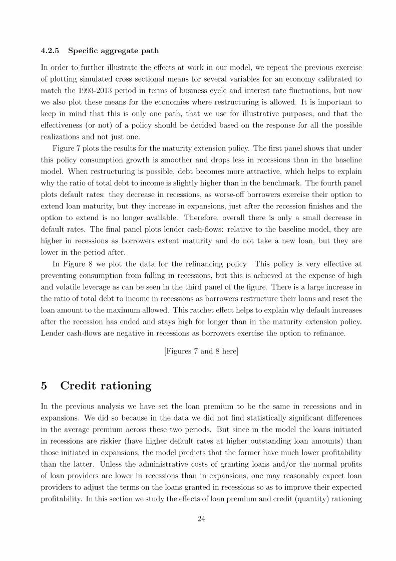
4.2.5 Specific aggregate path
In order to further illustrate the effects at work in our model, we repeat the previous exercise
of plotting simulated cross sectional means for several variables for an economy calibrated to
match the 1993-2013 period in terms of business cycle and interest rate fluctuations, but now
we also plot these means for the economies where restructuring is allowed. It is important to
keep in mind that this is only one path, that we use for illustrative purposes, and that the
effectiveness (or not) of a policy should be decided based on the response for all the possible
realizations and not just one.
Figure 7 plots the results for the maturity extension policy. The first panel shows that under
this policy consumption growth is smoother and drops less in recessions than in the baseline
model. When restructuring is possible, debt becomes more attractive, which helps to explain
why the ratio of total debt to income is slightly higher than in the benchmark. The fourth panel
plots default rates: they decrease in recessions, as worse-off borrowers exercise their option to
extend loan maturity, but they increase in expansions, just after the recession finishes and the
option to extend is no longer available. Therefore, overall there is only a small decrease in
default rates. The final panel plots lender cash-flows: relative to the baseline model, they are
higher in recessions as borrowers extent maturity and do not take a new loan, but they are
lower in the period after.
In Figure 8 we plot the data for the refinancing policy. This policy is very effective at
preventing consumption from falling in recessions, but this is achieved at the expense of high
and volatile leverage as can be seen in the third panel of the figure. There is a large increase in
the ratio of total debt to income in recessions as borrowers restructure their loans and reset the
loan amount to the maximum allowed. This ratchet effect helps to explain why default increases
after the recession has ended and stays high for longer than in the maturity extension policy.
Lender cash-flows are negative in recessions as borrowers exercise the option to refinance.
[Figures 7 and 8 here]
5 Credit rationing
In the previous analysis we have set the loan premium to be the same in recessions and in
expansions. We did so because in the data we did not find statistically significant differences
in the average premium across these two periods. But since in the model the loans initiated
in recessions are riskier (have higher default rates at higher outstanding loan amounts) than
those initiated in expansions, the model predicts that the former have much lower profitability
than the latter. Unless the administrative costs of granting loans and/or the normal profits
of loan providers are lower in recessions than in expansions, one may reasonably expect loan
providers to adjust the terms on the loans granted in recessions so as to improve their expected
profitability. In this section we study the effects of loan premium and credit (quantity) rationing
24
on loan profitability. We then evaluate the different restructuring policies in a setting where
risk-adjusted loan profitability is the same for loans granted in recessions and in expansions.
5.1 Prices versus quantities
There are at least two ways to (potentially) achieve higher profitability on the loans granted
in recessions. The first is to increase the loan premium. As previously discussed, in the data
we do not find strong evidence for it. The average loan premium is slightly higher in recessions
than in expansions, 8.6% compared to 8.1%, respectively, but the difference is not statistically
significant.
In spite of this evidence, we use our model to investigate the effects of increasing the premium
on loans granted in recessions. The solution to this more general model requires an additional
(binary) state variable, whether the currently outstanding loan (if any) was initiated in a
recession or in an expansion.
The results are shown in Table 12. We report results for a loan premium in recessions equal
to 8.0% (the baseline, Panel A), 8.6% (the value in the data, Panel B) and for a considerably
higher value of 15% (Panel C). Due to its higher cost, debt becomes less attractive as an
instrument to smooth consumption over time and across states. This leads to a reduction in
the demand for loans. The higher cost of debt also explains why the default probabilities are
now higher than before. Default rates increase during both recessions and expansions: some of
the loans on which there is default in expansions were granted in recessions and they carry a
higher premium. The lower attractiveness of debt leads borrowers to default earlier in the life
of the loan, at higher values of outstanding debt.
[Table 12 here]
The third row of each panel of Table 12 reports the annual default rates calculated using
loan/year as the unit of observation. That is: we calculate the proportion of loans outstanding
at the beginning of the period for which there is default in that period. Therefore, these default
rates are conditional on the business cycle upon default, i.e. whether the loan defaulted during
a recession or an expansion. These default probabilities can more easily be compared with
the (annual) default rates usually reported in the data. Since our loans are multiperiod, they
contribute to the calculation of annual default probabilities in more than one year (unless there
is immediate default).
We can also calculate default probabilities using one observation per loan. That is: we can
calculate the proportion of loans for which there is default over the whole life of the loan, also
conditional on the state of the business cycle at loan inception (and not at default). We report
them in the fourth row of each panel (these are not annual default probabilities).
When the loan premium for loans initiated in recession increases, so do the default proba-
bilities on these loans. The quantitative effects are significant: for an increase in loan premium
25
for loans granted in recessions from 8% to 15% there is an increase in their default rate from
13% to 21%. This helps to explain why in spite of the large increase in premium there is a rela-
tively smaller effect on the net present value of these loans, that increases from -0.025 to 0.211.
The latter value is still much lower than the net present value for loans granted in expansions
(at a premium of 8%). This shows that increases in the premium are somewhat ineffective in
improving loan profitability: as the premium increases the riskier borrowers are the ones who
will still demand credit, so that expected default rates and loan losses go up.
An alternative way for lenders to improve the profitability of loans granted in recessions is
to deny credit to the riskiest borrowers. We model a simple credit rationing rule: borrowers
with permanent income below a given threshold z are not able to take out a new loan in
recessions (they may still have debt outstanding from a loan taken out in an earlier period).
This rule could be implemented by requiring that borrowers present proof of their earnings (e.g.
payslips) prior to being approved for the loan.25 In terms of our model, it means that if the
(log) permanent income of borrower i in recession period t is such that:
zit < z (21)
then this borrower is not given a new loan. Since the level of permanent income is a state variable
of the model, the implementation of the above restriction does not require an additional state
variable. We solve endogenously for the cut-off z, so as to equate the risk-adjusted profitability
of the loans granted in recessions and in expansions. This cut-off is −0.45 which means that
during a recession 8% of the overall population of agents are excluded from the loan market.
This is 26% of the set of agents that do decide to take out a new loan.
The results are shown in Table 13. The probability of a new loan being granted in recessions
decreases, from 18% to 15%. Some of the borrowers who are refused credit during the recession
period eventually take out a new loan when aggregate economic conditions change. But in spite
of this, there still is a decline in the probability of a new loan being taken out in expansions.
The reason is that debt is now overall less attractive: borrowers will not be able to access a new
loan precisely in the states of the world when they may need it the most, when their income is
low. The lower attractiveness of debt helps to explain the small increase in annual default prob-
abilities. Recall that these annual recession (expansion) default probabilities include default by
loans that began in expansions (recessions).
[Table 13 here]
In the third row of Table 13 we report cumulative default probabilities for loans granted in
recessions/expansions (one observation per loan). As a result of riskier borrowers being denied
credit, default rates for loans that began in recessions drop considerably, from 13.3% to 6.2%.
25Payslips provide proof of total income and not of permanent income, the difference arising from temporary
fluctuations in income. In the model we consider a screening rule based on permanent income since it simplifies
considerably the solution of the model.
26

On the other hand, default rates for loans granted in expansions rise slightly, as some of the
risky agents who are excluded from borrowing in recessions shift their demand to expansions.
5.2 Restructuring policies
We now evaluate the effects of the different restructuring policies (interest rate reduction,
maturity extension, refinancing), but in a setting in which lenders engage in credit rationing
during recessions, so as to equate the profitability of loans granted at different stages of the
business cycle. For comparability, the results that we report for the different restructuring
policies are for the same level of credit rationing as above (i.e. borrowers with zit < −0.45 are
denied a new loan in recessions). As before, we let borrowers decide whether or not they wish
to take advantage of the policies, and we allow all borrowers (including those below the credit
rationing cut-off) to take advantage of them. We adjust the loan premium so that risk-adjusted
profitability is the same throughout.
The results are reported in Table 14. The first panel reports the results for the model where
debt restructuring is not possible, and the following panels reports the results for the different
restructuring policies.
[Table 14 here]
Focusing first on the maturity extension policy, the reduction in the loan premium so that
profitability remains the same is larger for loans initiated in expansions than for those initiated
in recessions. Cash-flow in recessions is more valuable than in expansions. Furthermore, the
option to extend loan maturity is more likely to be exercised for loans initiated in recessions.
Lenders need to be compensated for this through a higher loan interest rate. This is in spite
of the slightly higher default rates for loans initiated in expansions than for those initiated
in recessions. As before, the maturity extension policy allows borrowers to better smooth
consumption over time (smaller average consumption growth) and across the cycle (smaller
difference in average consumption growth across recessions and expansions). The policy leads
to a reduction in overall average lender cash-flows in recessions and an increase in expansions.
The proportion of recession periods in which lenders have negative cash-flows increases from
0.5 percent to 5.5 percent.
As before, the policy of allowing for a reduction in loan interest rate in bad times to 7%
is fairly ineffective (Panel C of Table 14). Ex-post all individuals will want to take advantage
of it. The loan premium, both for loans initiated in recession and expansion, must increase
to account for this, reducing the benefits of the policy along several dimensions (consumption
smoothing, borrower welfare, default probabilities).
Panel D reports the results for the refinancing policy. As before, from a borrower perspective,
this policy is the most effective. However, it comes at the expense of very volatile lender cash-
flows, which become on average very negative during recessions. Therefore, the main trade-offs
27

and conclusions are similar to the analysis in which lenders do not restrict borrowers’ access to
credit in bad times.
6 Conclusion
We have quantitatively evaluated the trade-offs of alternative consumer debt restructuring
policies. We have done so in the context of a dynamic model in which agents face earnings risk,
both of idiosyncratic and aggregate sources. Recessions are characterized by lower expected
earnings growth and a higher probability of a large drop in earnings. As a result, agents are more
likely to cutback on consumption during bad times and the demand for credit is procyclical.
However, those agents who experience the realization of a large drop in earnings in recessions
do want to borrow so that the pool of new borrowers becomes riskier. And those who have
previously outstanding debt are more likely to default, which explains the countercyclicality of
default rates.
Among the three debt restructuring policies that we have analyzed the one that leads to
better outcomes is loan maturity extension. It leads to slightly lower default rates, a smaller
drop in consumption in recessions, and increased borrower welfare. Interestingly, not all bor-
rowers decide to take up the option to extend the loan maturity. Only those who have lower
cash-on-hand do so. For the remainder, the lower expected earnings growth and the higher risk
that characterize recessions lead them to want to deleverage, also for precautionary reasons.
Under this policy lenders receive lower average but still positive cash-flows in recessions.
A loan modification policy characterized by a decrease in the loan interest rate in recessions
turns out to be too costly for lenders. Ex-post, i.e. when faced with the recession, all borrowers
wish to benefit from the reduction, regardless of their financial position. Lenders need to be
compensated for this ex-ante, so that the benefits of the policy are reduced. The final policy
that we have considered is to give borrowers the option to refinance the loan during bad times.
This involves taking out a new loan and repaying the previous one. Even though this policy
is very effective in reducing the effects of recessions on consumption and default, it has a very
large impact on the properties of the cash-flows of lenders. They become on average negative in
recessions and they have substantial downside risk. Therefore, given the trade-offs, the maturity
extension policy results in more balanced outcomes.
Our model provides important insights on the optimal clauses to be included on consumer
loan contracts. In particular, our analysis supports the idea that it would be beneficial for
lenders to include clauses that allow borrowers to extend the loan maturity in case of a recession.
This would contribute to a reduction in default rates and a smaller fall in consumption in
bad times, and potentially help to prevent or attenuate the downward spirals that seem to
characterize recessions. Policymakers also have an important role to play, by putting in place
the relevant legal and institutional framework that facilitates such restructuring of loans.
28

References
Adelino, M., K. Gerardi, and P. Willen (2013): “Why don’t lenders renegotiate more
home mortgages? Redefaults, self-cures and securitization,” Journal of Monetary Economics,
60(7), 835–853.
Alvarez, F., and U. Jermann (2000): “Efficiency, equilibrium, and asset pricing with risk
of default,” Econometrica, 68(4), 775–797.
Athreya, K. (2005): “Equilibrium Models of Personal Bankruptcy: A Survey,” Federal Re-
serve Bank of Richmond Quarterly, 91(2), 73–98.
Campbell, J. Y., and J. F. Cocco (2015): “A model of mortgage default,” The Journal of
Finance, 70(4), 1495–1554.
Chatterjee, S., D. Corbae, M. Nakajima, and J. Rios-Rull (2007): “A quantitative
theory of unsecured credit with risk of default,” Econometrica, 75(6), 1525–1589.
Chen, H., M. Michaux, and N. Roussanov (2013): “Houses as ATMs? Mortgage refi-
nancing and macroeconomic uncertainty,” Discussion paper, National Bureau of Economic
Research.
Constantinides, G. M., and D. Duffie (1996): “Asset pricing with heterogeneous con-
sumers,” Journal of Political economy, pp. 219–240.
Corbae, D., and E. Quintin (2015): “Leverage and the foreclosure crisis,” Journal of
Political Economy, 123(1), 1–65.
Deaton, A. (1991): “Saving and Liquidity Constraints,” Econometrica: Journal of the Econo-
metric Society, 59(5), 1221–1248.
Fay, S., E. Hurst, and M. White (2002): “The household bankruptcy decision,” American
Economic Review, 92(3), 706–718.
Gerardi, K. S., H. S. Rosen, and P. S. Willen (2010): “The impact of deregulation
and financial innovation on consumers: The case of the mortgage market,” The Journal of
Finance, 65(1), 333–360.
Gross, D. B., and N. S. Souleles (2002): “An empirical analysis of personal bankruptcy
and delinquency,” Review of Financial Studies, 15(1), 319–347.
Guerrieri, V., and G. Lorenzoni (2009): “Equilibrium Models of Personal Bankruptcy:
A Survey,” Econometrica, 77(6), 1751–1790.
Guiso, L., P. Sapienza, and L. Zingales (2013): “The determinants of attitudes toward
strategic default on mortgages,” The Journal of Finance, 68(4), 1473–1515.
29

Guvenen, F., S. Ozkan, and J. Song (2014): “The nature of countercyclical income risk,”
Journal of Political Economy, 122(3), 621–660.
Kiyotaki, N., and J. Moore (1997): “Credit cycles,” Journal of Political Economy, 105(2),
211–248.
Kocherlakota, N., and L. Pistaferri (2009): “Asset pricing implications of Pareto opti-
mality with private information,” Journal of Political Economy, 117(3), 555–590.
Kovrijnykh, N., and I. Livshits (2013): “Screening as a Unified Theory of Delinquency,
Renegotiation and Bankruptcy,” Working Paper.
Krusell, P., and A. A. Smith (1997): “Income and wealth heterogeneity, portfolio choice,
and equilibrium asset returns,” Macroeconomic dynamics, 1(02), 387–422.
Livshits, I. (2014): “Recent Developments in Consumer Credit and Default Literature,”
Working Paper.
Livshits, I., J. MacGee, and M. Tertilt (2007): “Consumer bankruptcy: A fresh start,”
The American Economic Review, 97(1), 402–418.
Mankiw, N. G. (1986): “The equity premium and the concentration of aggregate shocks,”
Journal of Financial Economics, 17(1), 211–219.
Mian, A., K. Rao, and A. Sufi (2013): “Household Balance Sheets, Consumption, and the
Economic Slump,” The Quarterly Journal of Economics, 128(4), 1687–1726.
Storesletten, K., C. I. Telmer, and A. Yaron (2007): “Asset pricing with idiosyncratic
risk and overlapping generations,” Review of Economic Dynamics, 10(4), 519–548.
Tauchen, G., and R. Hussey (1991): “Quadrature-based methods for obtaining approxi-
mate solutions to nonlinear asset pricing models,” Econometrica: Journal of the Econometric
Society, 59(2), 371–396.
30

A Appendices
A.1 Numerical Solution
We take the loan premium and the form of debt restructuring available as given and solve the
agent’s problem using backward induction. In the last period (t = T ) the policy functions are
trivial, the agent simply decides whether or not to default on the outstanding debt. Absent
the stigma cost agents would always default in the last period since the threat of exclusion
from credit markets no longer plays a role. In other words, in the last period the psychological,
legal and financial costs of default are the only mechanism preventing default. In case of no
default the agent repays the principal amount still outstanding and consumes his cash-on-hand.
In this period the value function corresponds to the indirect utility function. We then iterate
backwards.
For every period t prior to T , and for each combination of values for the state variables, we
optimize over the choice variables using a discrete grid search. We use an equally spaced grid for
cash-on-hand (Xt) and for the log level of permanent income (zt). The upper and lower bounds
for these grids were chosen to be non-binding at all times. And in order to improve accuracy and
efficiency of the solution we let the boundaries for the grid zt to increase from period t to T . The
density functions of the random variables (i.e. shocks to the earnings process and to interest
rates) were approximated using Gaussian quadrature (Tauchen and Hussey (1991)). For points
that do not lie on the state space grid, we evaluate the value function using a cubic spline
interpolation for the cash-on-hand grid and a linear interpolation for the permanent income
grid. We calculate the value function associated with all possible values for the choice/control
variables and optimize over these. In this way we obtain the optimal choices of consumption,
borrowing, default, and whether to restructure the loan.
We use the optimal choices of the agents to calculate the cash-flows of lenders. If their
present value is higher (lower) than in the baseline model where the option to restructure is
not available we decrease (increase) the loan premium and solve the agent’s problem again. We
repeat the process until we find a fixed point in which the present value of the risk-adjusted cash-
flows of lenders is the same in the model with restructuring and in the baseline model where
debt restructuring is not available. We repeat this process for each of the debt restructring
policies analyzed.
31

A.2 Data Description
In this section we describe the sources for the data that we use in the paper.
Household Debt - Data on US household debt is taken from the Federal Reserve Database,
namely from the Z.1 Financial Accounts (table L.100). Total Household Debt is the sum of
Mortgage Debt, Consumer Debt and Other.26
• Home Mortgages - Includes loans made under home equity lines of credit and home equity
loans secured by junior lien (unique identifier Z1/Z1/FL153165105.Q).
• Consumer Credit - Outstanding credit extended to individuals for household, family,
and other personal expenditures, excluding loans secured by real estate (unique identifier
Z1/Z1/FL153166000.Q).
• Other loans - Includes cash accounts at brokers and dealers and syndicated loans to
nonfinancial corporate business by nonprofits and domestic hedge funds (unique identifier
Z1/Z1/FL383169005.Q
Disposable Income, GDP, Inflation and Recession Periods
• Nominal GDP Data - The nominal GDP data is again from the Z.1 Financial Accounts
from the Federal Reserve (unique Identifier: Z1/Z1/FA086902005.Q).
• Disposable Income Data - The disposable income data is from the Bureau of Economic
Analysis (Table 2.1. Personal Income and Its Disposition)27
• Recession Periods - The recession periods are defined according to the NBER business
cycle dates.28
• Inflation Data - The inflation data is the Consumer Price Index for All Urban Consumers
from FRED (unique identifier: CPIAUCSL).29
• Expected Inflation Data - The expected inflation data is taken from the University of
Michigan Inflation Expectation Survey available from FRED (unique identifier: MICH).30
Credit Spreads
• Consumer Debt - We take data for interest rates on credit card plans, 24-month personal
loans and 48-months new car loans from the FED. Interest rates for new-car loans and
26The latest statistical release can be found here: http://www.federalreserve.gov/releases/Z1/Current/
z1.pdf27The FED uses data on Disposable Income from BEA on its calculations: http://www.federalreserve.
gov/releases/housedebt/about.htm.
Data can be found here: http://www.bea.gov/iTable/iTable.cfm?ReqID=9&step=1#reqid=9&step=3&
isuri=1&904=2014&903=58&906=q&905=1929&910=x&911=128http://www.nber.org/cycles.html29http://research.stlouisfed.org/fred2/series/CPIAUCSL#30https://research.stlouisfed.org/fred2/series/MICH
32

personal loans at commercial banks are simple unweighed averages of each bank’s most
common rate and for credit card accounts, the rate for all accounts is the stated APR
averaged across all credit card accounts at all reporting banks.
• Treasury Bills - t-bill rates are taken from the FED, except for the 1-month t-bill which
is from the Kenneth French library (i.e. from Ibbotson Associates) given this series is
longer than the FED.
Non-performing Loans - Data on charge-off rates and Delinquency rates is taken from FED.
The data is compiled quarterly by the Federal Financial Institutions Examination Council.31
The data on personal bankruptcy filling rates is from Administrative Office of the U.S. Courts
and the U.S. Census Bureau.32
• Charge-off rates - Charge-offs are the value of loans and leases removed from the books
and charged against loss reserves. The charge off rate is the net charge-off (gross charge-
offs minus recoveries) during a quarter divided by the average level of it loans outstanding
over that quarter. The figure is then annualized.
• Delinquency rates - Delinquent loans and leases are those past due thirty days or more
and still accruing interest as well as those in nonaccrual status. The delinquency ratio is
the ratio between the dollar amount of a bank’s delinquent loans to the dollar amount of
total loans outstanding. The rate is then annualized.
• Bankruptcy filling rates - Personal bankruptcy filling rates rates are the total number of
households who file for bankruptcy in the U.S. (annual non-business fillings) divided by
the total number of U.S. households.
31http://www.federalreserve.gov/releases/chargeoff/32http://www.uscourts.gov/report-name/bankruptcy-filings and http://www.abi.org/newsroom/
bankruptcy-statistics
33
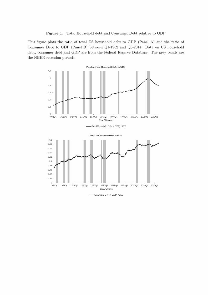
Figure 1: Total Household debt and Consumer Debt relative to GDP
This figure plots the ratio of total US household debt to GDP (Panel A) and the ratio of
Consumer Debt to GDP (Panel B) between Q1-1952 and Q3-2014. Data on US household
debt, consumer debt and GDP are from the Federal Reserve Database. The grey bands are
the NBER recession periods.
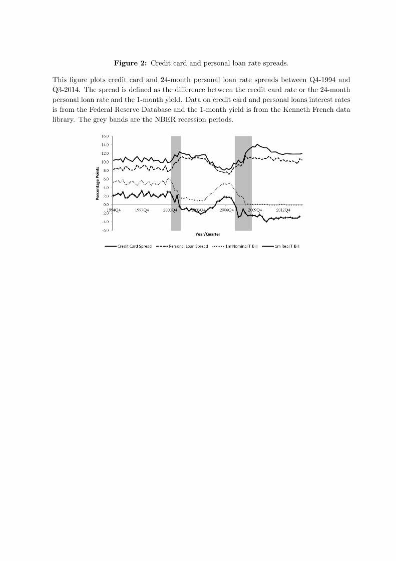
Figure 2: Credit card and personal loan rate spreads.
This figure plots credit card and 24-month personal loan rate spreads between Q4-1994 and
Q3-2014. The spread is defined as the difference between the credit card rate or the 24-month
personal loan rate and the 1-month yield. Data on credit card and personal loans interest rates
is from the Federal Reserve Database and the 1-month yield is from the Kenneth French data
library. The grey bands are the NBER recession periods.
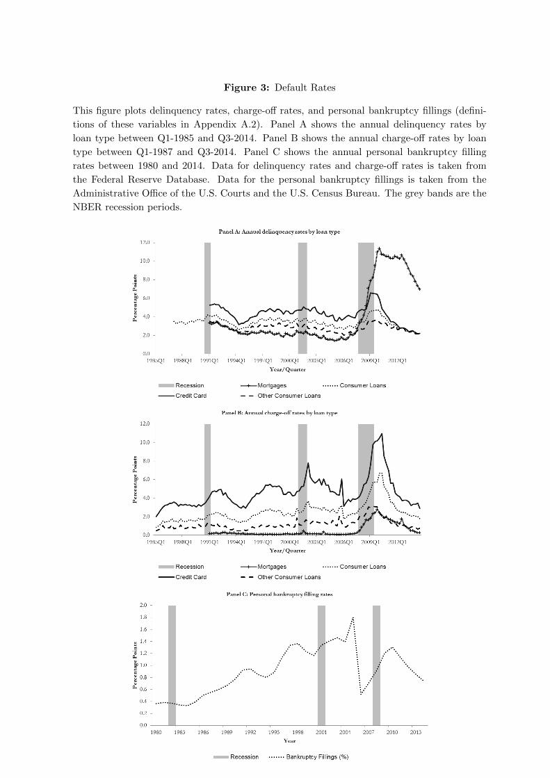
Figure 3: Default Rates
This figure plots delinquency rates, charge-off rates, and personal bankruptcy fillings (defini-
tions of these variables in Appendix A.2). Panel A shows the annual delinquency rates by
loan type between Q1-1985 and Q3-2014. Panel B shows the annual charge-off rates by loan
type between Q1-1987 and Q3-2014. Panel C shows the annual personal bankruptcy filling
rates between 1980 and 2014. Data for delinquency rates and charge-off rates is taken from
the Federal Reserve Database. Data for the personal bankruptcy fillings is taken from the
Administrative Office of the U.S. Courts and the U.S. Census Bureau. The grey bands are the
NBER recession periods.
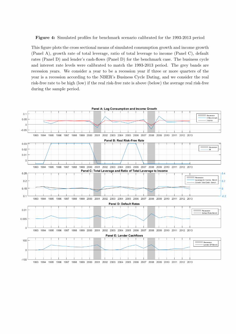
Figure 4: Simulated profiles for benchmark scenario calibrated for the 1993-2013 period
This figure plots the cross sectional means of simulated consumption growth and income growth
(Panel A), growth rate of total leverage, ratio of total leverage to income (Panel C), default
rates (Panel D) and lender’s cash-flows (Panel D) for the benchmark case. The business cycle
and interest rate levels were calibrated to match the 1993-2013 period. The grey bands are
recession years. We consider a year to be a recession year if three or more quarters of the
year is a recession according to the NBER’s Business Cycle Dating, and we consider the real
risk-free rate to be high (low) if the real risk-free rate is above (below) the average real risk-free
during the sample period.
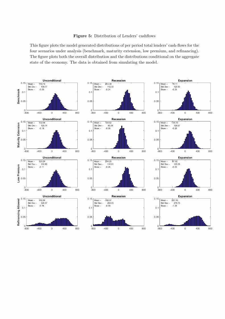
Figure 5: Distribution of Lenders’ cashflows
This figure plots the model generated distributions of per period total lenders’ cash-flows for the
four scenarios under analysis (benchmark, maturity extension, low premium, and refinancing).
The figure plots both the overall distribution and the distributions conditional on the aggregate
state of the economy. The data is obtained from simulating the model.

Figure 6: Mean-Preserving Spreads
This figure plots the lenders’ net present value per loan considering a decrease of the discount
rate in expansions and an increase of the discount rate in recessions while keeping the average
discount rate the same (mean-preserving spreads). The x-axis is the change in the expansion
discount rate. Panel A (Panel B) plots the NPVs discounted at the risk-free rate (risk-adjusted
discount rate) and the mean-preserving spread is applied to this rate.

Figure 7: Simulated profiles for benchmark and maturity extension scenarios calibrated for
the 1993-2013 period
This figure plots the cross sectional means of simulated consumption growth and income growth
(Panel A), growth rate of total leverage and ratio of total leverage to income (Panel C), default
rates (Panel D) and lender’s cash-flows (Panel E) for the benchmark (solid lines) and maturity
extension (dotted lines) scenarios. The business cycle and interest rate levels were calibrated
to match the 1993-2013 period. The grey bands are recession years. We consider a year to be
a recession year if three or more quarters of the year is a recession according to the NBER’s
Business Cycle Dating, and we consider the real risk-free rate to be high (low) if the real
risk-free rate is above (below) the average real risk-free during the sample period.

Figure 8: Simulated profiles for benchmark and refinancing scenarios calibrated for the 1993-
2013 period
This figure plots the cross sectional means of simulated consumption growth and income growth
(Panel A), growth rate of total leverage and ratio of total leverage to income (Panel C), default
rates (Panel D) and lender’s cash-flows (Panel E) for the benchmark (solid lines) and refinancing
(dotted lines) scenarios. The business cycle and interest rate levels were calibrated to match
the 1993-2013 period. The grey bands are recession years. We consider a year to be a recession
year if three or more quarters of the year is a recession according to the NBER’s Business
Cycle Dating, and we consider the real risk-free rate to be high (low) if the real risk-free rate
is above (below) the average real risk-free during the sample period.

Table 1: Baseline parameters.
This table reports the baseline model parameters.
Description Parameter Value
Panel A: Business Cycle Transition Probabilities
Prob (Recession | Recession) 0.37
Prob (Recession | Expansion) 0.18
Panel B: Labor Income Process
Log permanent income AR(1) coefficient ρ 0.979
Prob. aggregate/idiosyncratic shock p1 0.49
Mean log earnings growth expansion (1) µ1E 0.119
Mean log earnings growth expansion (2) µ2E -0.026
Mean log earnings growth recession (1) µ1R -0.102
Mean log earnings growth recession (2) µ2R 0.094
St. dev permament income shock (1) σ1 0.325
St. dev permament income shock (2) σ2 0.001
St. dev. temporary shock σε 0.186
Tax Rate φ 20%
Panel C: Time and Preference parameters
Subjective discount factor β 0.8
Risk aversion γ 2
Number of periods T 20
Bequest motive b 0
Panel D: Real Interest Rate
Mean log real rate µr 0.012
Log real rate AR(1) coefficient φr 0.825
St. dev. of real rate σr 0.018
Term-premiun ξ 0.005
Panel E: Consumer Loans
Loan premium ψ 8.00%
Loan amount K $10k
Loan maturity τ 5 years
Default utility penalty λ 0.160
Prepayment cost θP ∞

Table 2: Means of different variables over the business cycle.
This table reports the mean for several variables, also conditional on the economy being in
a recession or an expansion. The variables are defined in the appendix. We use the NBER
business cycle dates to define recession/expansion periods. The last column reports the t-
statistics for tests of the difference in means across recesssions/expansions. The symbols ***,
** and * denote statistical significance at the 1%, 5% and 10% levels, respectively.
Unconditional Recession Expansion t-stat Rec=Exp
Spread: Personal loan - 1m t-bill 8.52 8.10 8.60 0.92
Spread: Credit card loan - 1m t-bill 11.06 11.26 11.03 -0.55
Charge-off rate on cons. loans 2.50 3.18 2.41 -2.47**
Charge-off rate on credit card 4.63 5.50 4.51 -2.08*
Charge-off rate on other cons. loans 1.17 1.86 1.07 -3.74***
Delinquency rate on cons. loans 3.41 3.92 3.33 -4.55***
Delinquency rate on credit card 4.29 5.22 4.15 -4.79***
Delinquency Rate on other cons. loans 2.82 3.12 2.78 -3.14***
∆ (Cons. debt) 2.00 0.97 2.24 3.23***
∆ (Cons. debt/Disp. inc.) 0.39 -0.32 0.55 2.07**
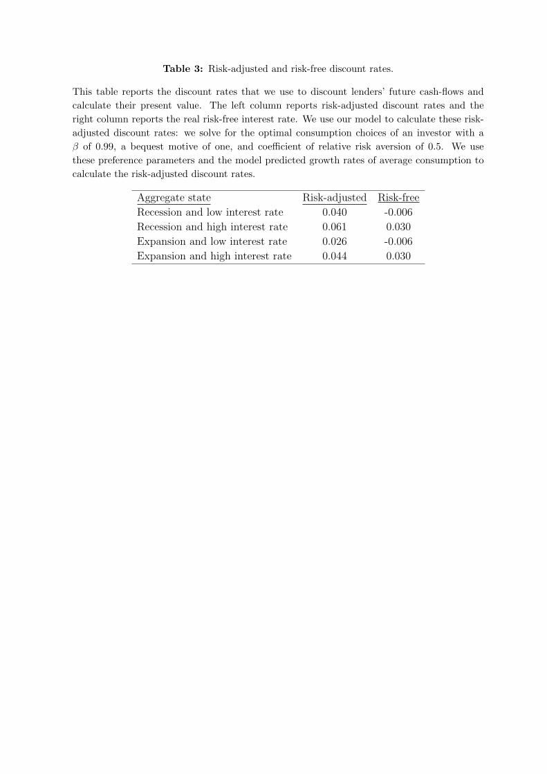
Table 3: Risk-adjusted and risk-free discount rates.
This table reports the discount rates that we use to discount lenders’ future cash-flows and
calculate their present value. The left column reports risk-adjusted discount rates and the
right column reports the real risk-free interest rate. We use our model to calculate these risk-
adjusted discount rates: we solve for the optimal consumption choices of an investor with a
β of 0.99, a bequest motive of one, and coefficient of relative risk aversion of 0.5. We use
these preference parameters and the model predicted growth rates of average consumption to
calculate the risk-adjusted discount rates.
Aggregate state Risk-adjusted Risk-free
Recession and low interest rate 0.040 -0.006
Recession and high interest rate 0.061 0.030
Expansion and low interest rate 0.026 -0.006
Expansion and high interest rate 0.044 0.030
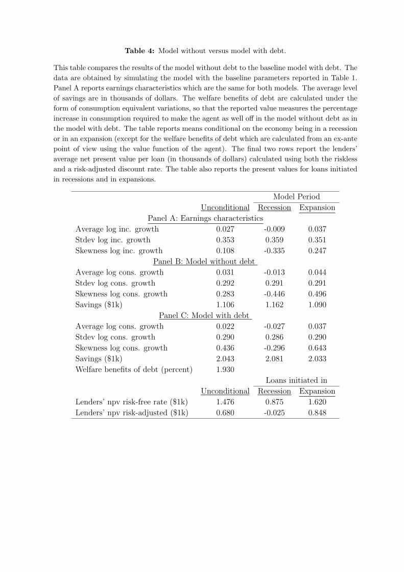
Table 4: Model without versus model with debt.
This table compares the results of the model without debt to the baseline model with debt. The
data are obtained by simulating the model with the baseline parameters reported in Table 1.
Panel A reports earnings characteristics which are the same for both models. The average level
of savings are in thousands of dollars. The welfare benefits of debt are calculated under the
form of consumption equivalent variations, so that the reported value measures the percentage
increase in consumption required to make the agent as well off in the model without debt as in
the model with debt. The table reports means conditional on the economy being in a recession
or in an expansion (except for the welfare benefits of debt which are calculated from an ex-ante
point of view using the value function of the agent). The final two rows report the lenders’
average net present value per loan (in thousands of dollars) calculated using both the riskless
and a risk-adjusted discount rate. The table also reports the present values for loans initiated
in recessions and in expansions.
Model Period
Unconditional Recession Expansion
Panel A: Earnings characteristics
Average log inc. growth 0.027 -0.009 0.037
Stdev log inc. growth 0.353 0.359 0.351
Skewness log inc. growth 0.108 -0.335 0.247
Panel B: Model without debt
Average log cons. growth 0.031 -0.013 0.044
Stdev log cons. growth 0.292 0.291 0.291
Skewness log cons. growth 0.283 -0.446 0.496
Savings ($1k) 1.106 1.162 1.090
Panel C: Model with debt
Average log cons. growth 0.022 -0.027 0.037
Stdev log cons. growth 0.290 0.286 0.290
Skewness log cons. growth 0.436 -0.296 0.643
Savings ($1k) 2.043 2.081 2.033
Welfare benefits of debt (percent) 1.930
Loans initiated in
Unconditional Recession Expansion
Lenders’ npv risk-free rate ($1k) 1.476 0.875 1.620
Lenders’ npv risk-adjusted ($1k) 0.680 -0.025 0.848
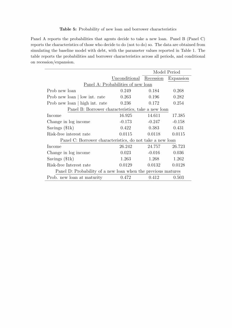
Table 5: Probability of new loan and borrower characteristics
Panel A reports the probabilities that agents decide to take a new loan. Panel B (Panel C)
reports the characteristics of those who decide to do (not to do) so. The data are obtained from
simulating the baseline model with debt, with the parameter values reported in Table 1. The
table reports the probabilities and borrower characteristics across all periods, and conditional
on recession/expansion.
Model Period
Unconditional Recession Expansion
Panel A: Probabilities of new loan
Prob new loan 0.249 0.184 0.268
Prob new loan | low int. rate 0.263 0.196 0.282
Prob new loan | high int. rate 0.236 0.172 0.254
Panel B: Borrower characteristics, take a new loan
Income 16.925 14.611 17.385
Change in log income -0.173 -0.247 -0.158
Savings ($1k) 0.422 0.383 0.431
Risk-free interest rate 0.0115 0.0118 0.0115
Panel C: Borrower characteristics, do not take a new loan
Income 26.242 24.757 26.723
Change in log income 0.023 -0.016 0.036
Savings ($1k) 1.263 1.268 1.262
Risk-free Interest rate 0.0129 0.0132 0.0128
Panel D: Probability of a new loan when the previous matures
Prob. new loan at maturity 0.472 0.412 0.503

Table 6: Probability of default and borrower characteristics
Panel A reports the probabilities that agents decide to default. Panel B (Panel C) reports the
characteristics of those who decide to default (not to default). The data are obtained from
simulating the baseline model with debt, with the parameter values reported in Table 1. The
table reports the probabilities and borrower characteristics across all periods, and conditional
on recession/expansion.
Model Period
Unconditional Recession Expansion
Panel A: Annual probabilities of default
Prob default 0.018 0.028 0.016
Prob default | low int. rate 0.016 0.025 0.014
Prob default | high int rate 0.021 0.031 0.018
Panel B: Borrower characteristics, default
Income 5.093 4.961 5.158
Change in log income -0.255 -0.354 -0.206
Outstanding debt 8.349 8.444 8.302
Risk-free interest rate 0.0140 0.0139 0.0141
Panel C: Borrower characteristics, do not default
Income 23.783 22.963 24.010
Change in log income 0.072 0.040 0.081
Outstanding debt 6.563 6.494 6.582
Risk-free interest rate 0.0118 0.0122 0.0117
Panel D: Probabilities of default per loan
Loans initiated in
Unconditional Recession Expansion
Prob default per loan 0.079 0.133 0.068
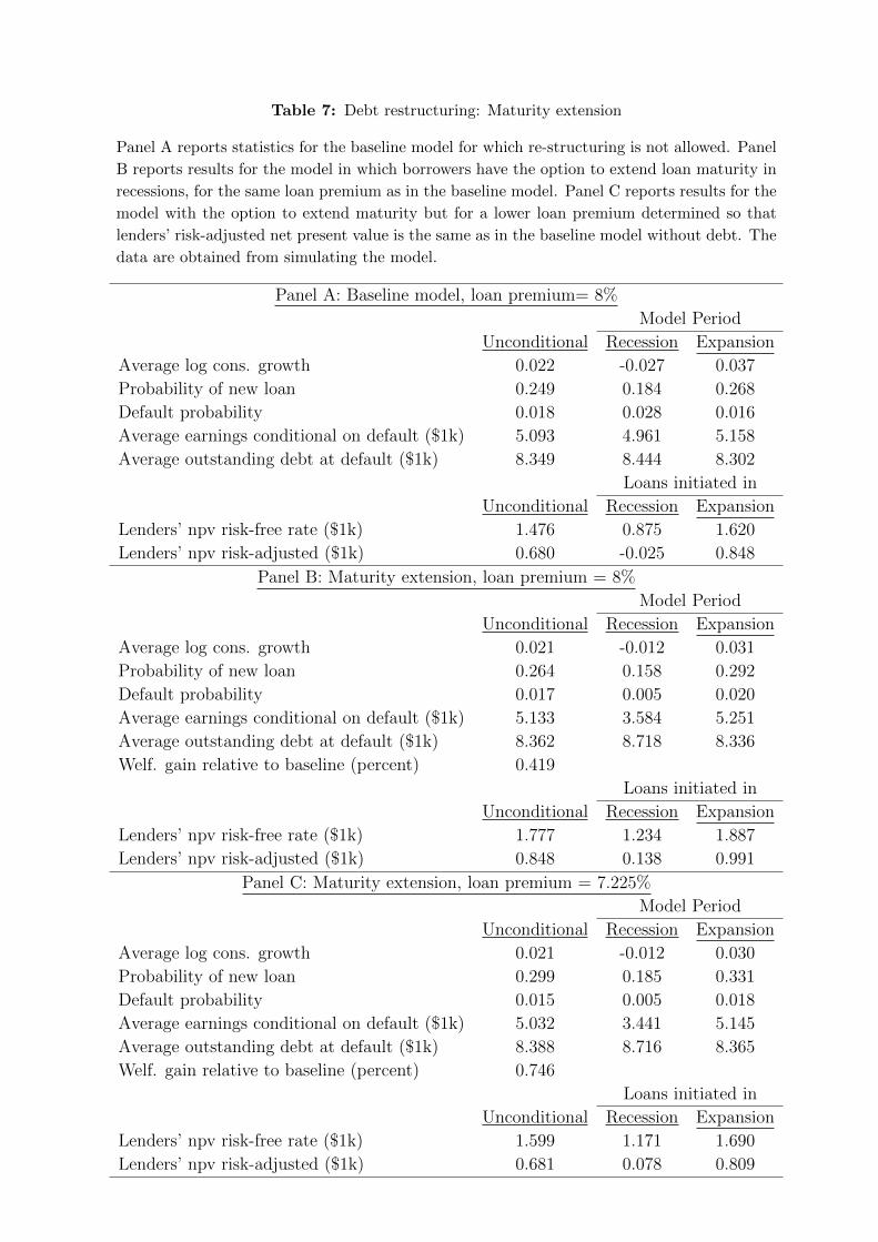
Table 7: Debt restructuring: Maturity extension
Panel A reports statistics for the baseline model for which re-structuring is not allowed. Panel
B reports results for the model in which borrowers have the option to extend loan maturity in
recessions, for the same loan premium as in the baseline model. Panel C reports results for the
model with the option to extend maturity but for a lower loan premium determined so that
lenders’ risk-adjusted net present value is the same as in the baseline model without debt. The
data are obtained from simulating the model.
Panel A: Baseline model, loan premium= 8%
Model Period
Unconditional Recession Expansion
Average log cons. growth 0.022 -0.027 0.037
Probability of new loan 0.249 0.184 0.268
Default probability 0.018 0.028 0.016
Average earnings conditional on default ($1k) 5.093 4.961 5.158
Average outstanding debt at default ($1k) 8.349 8.444 8.302
Loans initiated in
Unconditional Recession Expansion
Lenders’ npv risk-free rate ($1k) 1.476 0.875 1.620
Lenders’ npv risk-adjusted ($1k) 0.680 -0.025 0.848
Panel B: Maturity extension, loan premium = 8%
Model Period
Unconditional Recession Expansion
Average log cons. growth 0.021 -0.012 0.031
Probability of new loan 0.264 0.158 0.292
Default probability 0.017 0.005 0.020
Average earnings conditional on default ($1k) 5.133 3.584 5.251
Average outstanding debt at default ($1k) 8.362 8.718 8.336
Welf. gain relative to baseline (percent) 0.419
Loans initiated in
Unconditional Recession Expansion
Lenders’ npv risk-free rate ($1k) 1.777 1.234 1.887
Lenders’ npv risk-adjusted ($1k) 0.848 0.138 0.991
Panel C: Maturity extension, loan premium = 7.225%
Model Period
Unconditional Recession Expansion
Average log cons. growth 0.021 -0.012 0.030
Probability of new loan 0.299 0.185 0.331
Default probability 0.015 0.005 0.018
Average earnings conditional on default ($1k) 5.032 3.441 5.145
Average outstanding debt at default ($1k) 8.388 8.716 8.365
Welf. gain relative to baseline (percent) 0.746
Loans initiated in
Unconditional Recession Expansion
Lenders’ npv risk-free rate ($1k) 1.599 1.171 1.690
Lenders’ npv risk-adjusted ($1k) 0.681 0.078 0.809

Table 8: Debt restructuring: Summary statistics.
This table reports several summary statistics for the model with the different restructuring
policies. For comparison, the first column reports results for the baseline model in which
restructuring is not allowed. Panel A reports the proportion of borrowers who take up the
option to restructure the loan. Panel B reports the proportion of borrowers who decide to take
a new loan at maturity. Panel C (Panel D) reports average earnings for those who decide to
restructure (take or not a new loan at maturity). Panel E reports the overall distribution of
outstanding loan amounts (including both recessions and expansions). The table shows results
for the restructuring scenarios in which lenders’ risk-adjusted net present value is the same as
in the baseline model without debt. The data are obtained from simulating the model.
Baseline Mat. Ext. Low rate Refinancing
Prop. who exerc. option to restr. n/a 0.57 1.00 0.66
Panel A: Proportion who restructure, by outstanding loan amount
Amount = 10 n/a 0.80 1.00 0.79
8<Amount<10 n/a 0.66 1.00 0.66
6<Amount<8 n/a 0.49 1.00 0.55
4<Amount<6 n/a 0.25 1.00 0.37
2<Amount<4 n/a 0.51 1.00 n/a
Panel B: Probability of new loan at maturity
Recession 0.41 0.45 0.45 0.48
Expansion 0.50 0.57 0.54 0.57
Panel C: Average earn. for those who restructure, by outst. loan amount
Amount = 10 n/a 15.32 20.32 14.95
8<Amount<10 n/a 15.77 21.65 15.68
6<Amount<8 n/a 16.19 22.78 15.59
4<Amount<6 n/a 16.90 23.63 15.17
2<Amount<4 n/a 20.32 24.00 n/a
Panel D: Average earnings by decision to take a new loan at maturity
New loan given recession 14.74 14.38 14.88 16.30
No new loan given recession 31.45 38.40 31.59 34.72
New loan given expansion 17.50 17.66 17.52 18.55
No new loan given expansion 34.57 35.80 34.97 37.80
Panel E: Dist. of outstanding loan amount, given no previous default
Amount = 10 0.13 0.16 0.13 0.21
8<Amount<10 0.12 0.14 0.12 0.16
6<Amount<8 0.12 0.13 0.11 0.13
4<Amount<6 0.11 0.11 0.11 0.11
2<Amount<4 0.10 0.12 0.10 0.10
Amount = 0 0.42 0.34 0.43 0.30

Table 9: Debt restructuring: Low rate
Panel A reports statistics for the baseline model for which re-structuring is not allowed. Panel
B reports results for the model in which borrowers have the option to benefit from a reduction
of 1% in the loan interest rate in recessions. Panel C reports results for a model with the option
of a lower rate in recessions, but with a higher loan premium determined so that lenders’ risk-
adjusted net present value is the same as in the baseline model without debt. The data are
obtained from simulating the model.
Panel A: Baseline model, loan premium = 8%
Model Period
Unconditional Recession Expansion
Average log cons. growth 0.022 -0.027 0.037
Probability of new loan 0.249 0.184 0.268
Default probability 0.018 0.028 0.016
Average earnings conditional on default ($1k) 5.093 4.961 5.158
Average outstanding debt at default ($1k) 8.349 8.444 8.302
Loans initiated in
Unconditional Recession Expansion
Lenders’ npv risk-free rate ($1k) 1.476 0.875 1.620
Lenders’ npv risk-adjusted ($1k) 0.680 -0.025 0.848
Panel B: Loan premium = 8%, reduced by 1% in recessions
Model Period
Unconditional Recession Expansion
Average log cons. growth 0.022 -0.026 0.036
Probability of new loan 0.261 0.198 0.280
Default probability 0.018 0.026 0.016
Average earnings conditional on default ($1k) 5.064 4.883 5.148
Average outstanding debt at default ($1k) 8.354 8.492 8.291
Welf. gain relative to baseline (percent) 0.087
Loans initiated in
Unconditional Recession Expansion
Lenders’ npv risk-free rate ($1k) 1.446 0.894 1.583
Lenders’ npv risk-adjusted ($1k) 0.649 -0.011 0.813
Panel C: Loan premium = 8.25%, reduced by 1.25% in recessions
Model Period
Unconditional Recession Expansion
Average log cons. growth 0.022 -0.026 0.036
Probability of new loan 0.256 0.193 0.274
Default probability 0.018 0.026 0.016
Average earnings conditional on default ($1k) 5.074 4.886 5.159
Average outstanding debt at default ($1k) 8.370 8.494 8.314
Welf. gain relative to baseline (percent) 0.044
Loans initiated in
Unconditional Recession Expansion
Lenders’ npv risk-free rate ($1k) 1.485 0.894 1.630
Lenders’ npv risk-adjusted ($1k) 0.685 -0.011 0.856

Table 10: Debt restructuring: Refinance
Panel A reports statistics for the baseline model for which re-structuring is not allowed. Panel
B (and Panel C) report results for the model in which borrowers have the option to refinance
the loan in recessions, meaning that they are allowed to take a new one but must use the
proceeds to repay any previously outstanding debt. Panel B reports results for the same loan
premium as the baseline model and Panel C for a lower loan premium determined so that
lenders’ risk-adjusted net present value is the same as in the baseline model without debt. The
data are obtained from simulating the model.
Panel A: Baseline model, loan premium = 8%
Model Period
Unconditional Recession Expansion
Average log cons. growth 0.022 -0.027 0.037
Probability of new loan 0.249 0.184 0.268
Default probability 0.018 0.028 0.016
Average earnings conditional on default ($1k) 5.093 4.961 5.158
Average outstanding debt at default ($1k) 8.349 8.444 8.302
Loans initiated in
Unconditional Recession Expansion
Lenders’ npv risk-free rate ($1k) 1.476 0.875 1.620
Lenders’ npv risk-adjusted ($1k) 0.680 -0.025 0.848
Panel B: Refinance, loan premium = 8%
Model Period
Unconditional Recession Expansion
Average log cons. growth 0.020 0.003 0.025
Probability of new loan 0.284 0.218 0.303
Default probability 0.017 0.005 0.020
Average earnings conditional on default ($1k) 5.168 3.760 5.276
Average outstanding debt at default ($1k) 8.665 10.000 8.562
Welf. gain relative to baseline (percent) 0.723
Loans initiated in
Unconditional Recession Expansion
Lenders’ npv risk-free rate ($1k) 2.081 1.730 2.173
Lenders’ npv risk-adjusted ($1k) 0.989 0.457 1.128
Panel C: Refinance, loan premium = 6.875%
Model Period
Unconditional Recession Expansion
Average log cons. growth 0.020 0.005 0.024
Probability of new loan 0.327 0.255 0.347
Default probability 0.015 0.004 0.018
Average earnings conditional on default ($1k) 5.044 3.506 5.143
Average outstanding debt at default ($1k) 8.698 10.000 8.614
Welf. gain relative to baseline (percent) 1.165
Loans initiated in
Unconditional Recession Expansion
Lenders’ npv risk-free rate ($1k) 1.797 1.539 1.867
Lenders’ npv risk-adjusted ($1k) 0.692 0.252 0.811

Table 11: Properties of lender cash-flows
This table reports summary statistics on the properties of lenders’ per period cash-flows, both
overall and conditional on the aggregate state of the economy, for the baseline model and
for the models where restructuring is allowed. Panels A. B, and C report average, standard
deviation, and skewness of cash-flows, respectively. Panel D reports the proportion of periods
in which lenders have negative cash-flows. The data are obtained from simulating the model.
Unconditional Recession Expansion
Panel A: Mean cashflow (per period)
Baseline 118.15 255.39 79.11
Maturity extension 132.04 108.62 138.70
Low rate 120.25 234.25 87.82
Refinancing 142.35 -192.06 237.45
Panel B: Std. deviation of cashflow
Baseline 139.77 112.33 120.93
Maturity extension 120.74 93.39 126.66
Low rate 132.80 110.81 120.05
Refinancing 326.37 253.43 278.75
Panel C: Skewness cashflows
Baseline -0.03 -0.24 -0.25
Maturity extension -0.18 -0.08 -0.26
Low rate -0.11 -0.26 -0.25
Refinancing -0.76 -0.09 -1.28
Panel D: Proportion of periods with negative cashflows
Baseline 0.200 0.020 0.260
Maturity extension 0.140 0.120 0.140
Low rate 0.190 0.030 0.230
Refinancing 0.270 0.730 0.140

Table 12: Credit Rationing: Increasing Loan Premium in Recessions
This table reports statistics for the model in which the loan premium is increased for loans
taken in recessions. Panel A reports statistics for the baseline model in which the premium is
8.00% for both loans taken in recession and expansions. Panel B (Panel C) reports statistics for
the model in which the premium for loans taken in recessions is increased to 8.60% (15.00%).
The first three rows of each panel report means conditional on the economy being in a recession
or expansion. The last row of each panel reports means conditional on the business cycle at
loan initiation. The data are obtained from simulating the model.
Panel A: Loan Premium in Recessions: 8.00%
Model Period
Unconditional Recession Expansion
Average log cons. growth 0.022 -0.027 0.037
Probability of new loan 0.249 0.184 0.268
Default rates (annual) 0.018 0.028 0.016
Outstand. debt at default 8.349 8.444 8.302
Loans initiated in
Unconditional Recession Expansion
Default rates (per loan) 0.079 0.133 0.068
Lenders npv risk-adjusted 0.680 -0.025 0.848
Panel B: Loan Premium in Recessions: 8.60%
Model Period
Unconditional Recession Expansion
Average log cons. growth 0.022 -0.027 0.037
Probability of new loan 0.244 0.177 0.264
Default rates (annual) 0.019 0.028 0.016
Outstand. debt at default 8.390 8.484 8.343
Loans initiated in
Unconditional Recession Expansion
Default rates (per loan) 0.080 0.140 0.069
Lenders npv risk-adjusted 0.671 -0.021 0.841
Panel C: Loan Premium in Recessions: 15.00%
Model Period
Unconditional Recession Expansion
Average log cons. growth 0.023 -0.026 0.037
Probability of new loan 0.203 0.134 0.223
Default rates (annual) 0.022 0.033 0.019
Outstand. debt at default 8.664 8.751 8.622
Loans initiated in
Unconditional Recession Expansion
Default rates (per loan) 0.092 0.208 0.072
Lenders npv risk-adjusted 0.701 0.211 0.790
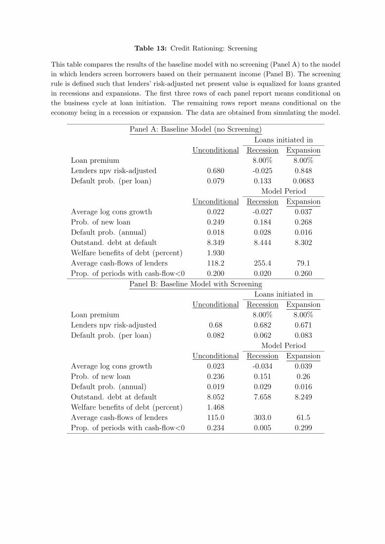
Table 13: Credit Rationing: Screening
This table compares the results of the baseline model with no screening (Panel A) to the model
in which lenders screen borrowers based on their permanent income (Panel B). The screening
rule is defined such that lenders’ risk-adjusted net present value is equalized for loans granted
in recessions and expansions. The first three rows of each panel report means conditional on
the business cycle at loan initiation. The remaining rows report means conditional on the
economy being in a recession or expansion. The data are obtained from simulating the model.
Panel A: Baseline Model (no Screening)
Loans initiated in
Unconditional Recession Expansion
Loan premium 8.00% 8.00%
Lenders npv risk-adjusted 0.680 -0.025 0.848
Default prob. (per loan) 0.079 0.133 0.0683
Model Period
Unconditional Recession Expansion
Average log cons growth 0.022 -0.027 0.037
Prob. of new loan 0.249 0.184 0.268
Default prob. (annual) 0.018 0.028 0.016
Outstand. debt at default 8.349 8.444 8.302
Welfare benefits of debt (percent) 1.930
Average cash-flows of lenders 118.2 255.4 79.1
Prop. of periods with cash-flow<0 0.200 0.020 0.260
Panel B: Baseline Model with Screening
Loans initiated in
Unconditional Recession Expansion
Loan premium 8.00% 8.00%
Lenders npv risk-adjusted 0.68 0.682 0.671
Default prob. (per loan) 0.082 0.062 0.083
Model Period
Unconditional Recession Expansion
Average log cons growth 0.023 -0.034 0.039
Prob. of new loan 0.236 0.151 0.26
Default prob. (annual) 0.019 0.029 0.016
Outstand. debt at default 8.052 7.658 8.249
Welfare benefits of debt (percent) 1.468
Average cash-flows of lenders 115.0 303.0 61.5
Prop. of periods with cash-flow<0 0.234 0.005 0.299
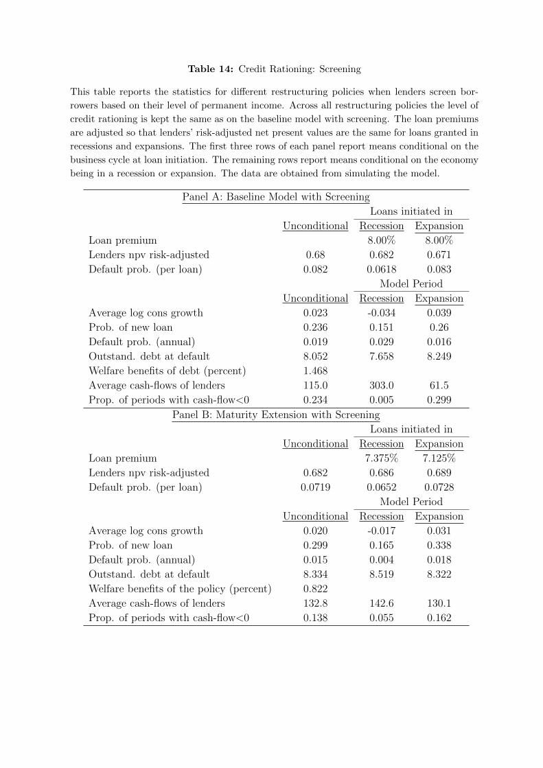
Table 14: Credit Rationing: Screening
This table reports the statistics for different restructuring policies when lenders screen bor-
rowers based on their level of permanent income. Across all restructuring policies the level of
credit rationing is kept the same as on the baseline model with screening. The loan premiums
are adjusted so that lenders’ risk-adjusted net present values are the same for loans granted in
recessions and expansions. The first three rows of each panel report means conditional on the
business cycle at loan initiation. The remaining rows report means conditional on the economy
being in a recession or expansion. The data are obtained from simulating the model.
Panel A: Baseline Model with Screening
Loans initiated in
Unconditional Recession Expansion
Loan premium 8.00% 8.00%
Lenders npv risk-adjusted 0.68 0.682 0.671
Default prob. (per loan) 0.082 0.0618 0.083
Model Period
Unconditional Recession Expansion
Average log cons growth 0.023 -0.034 0.039
Prob. of new loan 0.236 0.151 0.26
Default prob. (annual) 0.019 0.029 0.016
Outstand. debt at default 8.052 7.658 8.249
Welfare benefits of debt (percent) 1.468
Average cash-flows of lenders 115.0 303.0 61.5
Prop. of periods with cash-flow<0 0.234 0.005 0.299
Panel B: Maturity Extension with Screening
Loans initiated in
Unconditional Recession Expansion
Loan premium 7.375% 7.125%
Lenders npv risk-adjusted 0.682 0.686 0.689
Default prob. (per loan) 0.0719 0.0652 0.0728
Model Period
Unconditional Recession Expansion
Average log cons growth 0.020 -0.017 0.031
Prob. of new loan 0.299 0.165 0.338
Default prob. (annual) 0.015 0.004 0.018
Outstand. debt at default 8.334 8.519 8.322
Welfare benefits of the policy (percent) 0.822
Average cash-flows of lenders 132.8 142.6 130.1
Prop. of periods with cash-flow<0 0.138 0.055 0.162

Table 14 - continued
Panel C: Low Premium in recessions (7%) and Screening
Loans initiated in
Unconditional Recession Expansion
Loan premium 9.400% 8.500%
Lenders npv risk-adjusted 0.69 0.689 0.693
Default prob. (per loan) 0.0796 0.061 0.0828
Model Period
Unconditional Recession Expansion
Average log cons growth 0.022 -0.032 0.038
Prob. of new loan 0.239 0.156 0.263
Default prob. (annual) 0.019 0.028 0.016
Outstand. debt at default 8.054 7.614 8.26
Welfare benefits of the policy (percent) 0.005
Average cash-flows of lenders 116.6 281.4 69.7
Prop. of periods with cash-flow<0 0.220 0.007 0.281
Panel D: Refinancing and Screening
Loans initiated in
Unconditional Recession Expansion
Loan premium 8.250% 6.375%
Lenders npv risk-adjusted 0.685 0.685 0.685
Default prob. (per loan) 0.0726 0.0954 0.0681
Model Period
Unconditional Recession Expansion
Average log cons growth 0.019 0.003 0.024
Prob. of new loan 0.332 0.244 0.357
Default prob. (annual) 0.014 0.004 0.017
Outstand. debt at default 8.695 10.000 8.617
Welfare benefits of the policy (percent) 1.085
Average cash-flows of lenders 139.5 -180.8 230.5
Prop. of periods with cash-flow<0 0.262 0.680 0.143
Top Related