


Languages
Pages
Legal

AIRFOIL OPTIMIZATION FOR MORPHING AIRCRAFT
A Thesis
Submitted to the Faculty
of
Purdue University
by
Howoong Namgoong
In Partial Fulfillment of the
Requirements for the Degree
of
Doctor of Philosophy
December 2005

ii
I dedicate this thesis to my father, Young Kyu Namgoong in heaven.
iii
ACKNOWLEDGMENTS
Thanks to God for being my guidance of the journey of life.
It has been a privilege to be a student of Drs. William A. Crossley and Anastasios S.
Lyrintzis. I was able to open my eyes toward the world of design optimization and
morphing aircraft with a tremendous help from Dr. Crossley. I learned great knowledge
about aerodynamics and received precious advice from Dr. Lyrintzis. I will cherish and
miss the moments that we met together for five years.
Special thanks to my committee members, Dr. Scott D. King, Dr. Marc H. Williams
and Dr. Terrence A. Weisshaar for their invaluable comments and lectures. I also thank to
my colleagues and staffs in Purdue AAE department. This work was partially supported
by the Air Force Research Laboratory, contract F33615-00-C-3051, and by a Purdue
Research Foundation grant.
I would like to share this great moment with my lovely wife, Miran who completes
my life, and my beautiful son, Young who gives me another reason for living. I will not
forget the support from my three sisters, Ran, Eun and Yoon and my brothers in law. I
also like to thank my father and mother in law for their support and prayer.
Lastly, my deep appreciation goes to my mother, Mal Soon Park who showed me the
meaning of true love.
iv
TABLE OF CONTENTS
Page
LIST OF TABLES........................................................................................................... viii
LIST OF FIGURES ........................................................................................................... ix
ABSTRACT...................................................................................................................... xv
CHAPTER 1 INTRODUCTION ....................................................................................... 1
1.1 Background.............................................................................................................. 1
1.1.1 Airfoil Design Methods .................................................................................... 1
1.2 Issues in Airfoil Design Optimization ..................................................................... 4
1.2.1 Objective and Constraint Functions.................................................................. 4
1.2.2 Design Variables............................................................................................... 5
1.2.3 Global Optimization.......................................................................................... 9
1.2.4 Flow Models ..................................................................................................... 9
1.3 Morphing Aircraft.................................................................................................. 11
1.3.1 Return to the First Flight................................................................................. 11
1.3.2 Definition of Morphing Aircraft ..................................................................... 12
1.3.3 Morphing Aircraft Related Programs ............................................................. 12
1.4 Motivation of Research.......................................................................................... 17
1.4.1 Global Optimization Issues in Airfoil Optimization....................................... 17
1.4.2 Morphing Airfoil Design ................................................................................ 18
v
Page
1.5 Thesis Objectives ................................................................................................... 19
1.6 Thesis Organization ............................................................................................... 19
CHAPTER 2 TRANSONIC AIRFOIL OPTIMIZATION.............................................. 21
2.1 Design Variables.................................................................................................... 22
2.2 Base Airfoils .......................................................................................................... 28
2.3 Trimming ............................................................................................................... 31
2.4 Objective Function................................................................................................. 32
2.5 Accuracy of Function Evaluations......................................................................... 33
2.6 Computational Cost ............................................................................................... 38
2.6.1 Parallel Genetic Algorithm ............................................................................. 38
2.6.2 Gradient Based Optimization Method ............................................................ 40
2.7 Objectives and Fitness Function Formulation ....................................................... 40
2.7.1 Objectives ....................................................................................................... 40
2.7.2 Fitness Function Formulation ......................................................................... 41
2.8 Single-point Optimization Results Comparison .................................................... 43
2.8.1 GA Results ...................................................................................................... 43
2.8.2 GM Results ..................................................................................................... 53
2.9 Multi-point Optimization Results Comparison...................................................... 57
2.10 Lessons Learned from GA and GM Results ........................................................ 62
2.10.1 Multimodal Design Space............................................................................. 62
2.10.2 Computational Efficiency ............................................................................. 63
2.11 Summary .............................................................................................................. 64
CHAPTER 3 AIRFOIL OPTIMIZATION FOR MORPHING AIRCRAFT.................. 65
3.1 Problem Description .............................................................................................. 65
vi
Page
3.2 Objective Function Formulation ............................................................................ 67
3.2.1 Aerodynamics Only Investigation (Single-objective Approach).................... 67
3.2.2 Energy Based Optimization (Multi-objective Approach)............................... 68
3.2.3 Multi-objective Optimization.......................................................................... 69
3.3 Design Variables.................................................................................................... 72
3.3.1 Optimization Algorithm.................................................................................. 73
3.3.2 Flow Solver..................................................................................................... 73
3.4 Optimization Results.............................................................................................. 74
3.4.1 Aerodynamic-only Optimization Results ....................................................... 74
3.4.2 Energy Based Optimization Results ............................................................... 76
3.4.3 Cp and Energy Comparison............................................................................. 82
3.5 Transonic Morphing Airfoil................................................................................... 88
3.5.1 Problem Definition.......................................................................................... 88
3.5.2 Objective Function.......................................................................................... 88
3.5.3 Flow Solver, Design method and Parameters ................................................. 89
3.5.4 Aerodynamics-only Result.............................................................................. 89
3.5.5 Energy-based Design Results ......................................................................... 91
3.6 Summary ................................................................................................................ 99
CHAPTER 4 ACTUATION ENERGY MODELING INCLUDING AERODYNAMIC
WORK .................................................................................................... 100
4.1 Description of Concept ........................................................................................ 100
4.2 Formulation.......................................................................................................... 103
4.3 Sensorcraft Problem............................................................................................. 106
4.3.1 Problem Definition........................................................................................ 106
4.3.2 Stiffness Approximation ............................................................................... 107
4.4 Results and Comparison ...................................................................................... 109
vii
Page
4.4.1 Effect of Aerodynamic Work Term.............................................................. 109
4.4.2 Effect of Stiffness Change ............................................................................ 122
4.5 Summary .............................................................................................................. 130
CHAPTER 5 CONCLUSIONS ..................................................................................... 131
5.1 Future Directions ................................................................................................. 132
5.2 Contributions........................................................................................................ 133
LIST OF REFERENCES................................................................................................ 134
VITA............................................................................................................................... 139
viii
LIST OF TABLES
Table Page
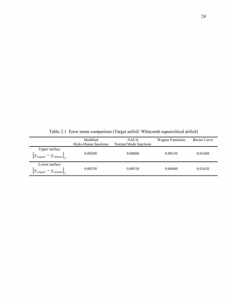
Table 2.1 Error norm comparison (Target airfoil: Whitcomb supercritical airfoil) ....... 24
Table 2.2 N-S solution comparison with experimental data........................................... 34
Table 2.3 Problem formulations ..................................................................................... 40
Table 2.4 Optimization methods..................................................................................... 42
Table 2.5 Single-point design result (GA)...................................................................... 44
Table 2.6 Single-point design result (GM) ..................................................................... 54
Table 2.7 Multi-point design result................................................................................. 57
Table 2.8 Comparisons of drag values and computational costs for GA and GM, (single-
point runs) ....................................................................................................... 63
Table 3.1 Airfoil design conditions ................................................................................ 66
Table 3.2 Drag comparison of aerodynamics only design.............................................. 74
Table 3.3 Drag and Relative Strain Energy comparison (weighted sum method).......... 76
Table 3.4 Drag and Relative Strain Energy comparison (ε-constraint method) ............. 78
Table 3.5 Transonic Morphing UAV Mission Profile .................................................... 88
Table 3.6 ε-constraint target values for Cd constraints ................................................... 97
Table 4.1 Actuation energy formulation....................................................................... 110
ix
LIST OF FIGURES
Figure Page
Figure 1.1 Discrete approach using airfoil coordinates ................................................... 6
Figure 1.2 Bezier approach using control points ............................................................. 7
Figure 1.3 The hierarchy of mathematical models ........................................................ 10
Figure 1.4 Front-view of Wright Flyer, illustrating wing warping (From Combs, Kill
Devil Hill, Houghton Mifflin, Boston,1979.) .............................................. 11
Figure 1.5 MAW modifications to F-111 (From NASA TM-4606).............................. 13
Figure 1.6 Flight-determined drag polar comparison (From NASA TM-4606)............ 13
Figure 1.7 Smart Technologies ...................................................................................... 14
Figure 1.8 Morphing airplane (NASA).......................................................................... 15
Figure 1.9 Sliding skins concept (Image: NextGen)...................................................... 16
Figure 1.10 Folding wing concept (Image: Lockheed Martin)........................................ 16
Figure 2.1 Shape functions ............................................................................................ 25
Figure 2.2 Original versus reconstructed airfoils........................................................... 26
Figure 2.3 NACA0012 with each shape function applied ............................................. 27
Figure 2.4 Configuration of base airfoils....................................................................... 28
Figure 2.5 Design space available using the NACA0012 base airfoil........................... 29
Figure 2.6 Design space available using the RAE2822 base airfoil .............................. 30
Figure 2.7 Design space available using the Whitcomb base airfoil ............................. 30
Figure 2.8 Schematics of trimming process................................................................... 32
Figure 2.9 Grid using 79 by 29 points (RAE2822 airfoil)............................................. 35
Figure 2.10 Grid using 129 by 30 points (RAE2822 airfoil)........................................... 35
Figure 2.11 Grid using 217 by 61 points (RAE2822 airfoil)........................................... 36
x
Figure Page
Figure 2.12 Pressure coefficient distribution of N-S prediction vs. published experiment
(RAE 2822 airfoil, M=0.74, α =3.19°) ....................................................... 36
Figure 2.13 Lift coefficient convergence history............................................................. 37
Figure 2.14 Drag coefficient convergence history........................................................... 37
Figure 2.15 Speed-up of parallel GA, computational wall time vs. number of CPUs..... 39
Figure 2.16 Best fitness value convergence history for all three GA runs. ..................... 44
Figure 2.17 Best airfoil shapes (top) and pressure coefficient distributions (bottom) in
selected generations of the GA using the NACA 0012 base airfoil. ........... 45
Figure 2.18 Best airfoil shapes (top) and pressure coefficient distributions (bottom) in
selected generations of the GA using the RAE 2822 base airfoil................ 46
Figure 2.19 Best airfoil shapes (top) and pressure coefficient distributions (bottom) in
selected generations of the GA using the Whitcomb supercritical base
airfoil............................................................................................................ 47
Figure 2.20 Mach contour for the NACA0012 airfoil (M=0.74, Cl=0.605, 64.12=α )
(top) and Mach contour for the best airfoil shape from 80th generations of
GA runs using the NACA0012 base airfoil (M=0.74, Cl=0.733)(bottom) .. 48
Figure 2.21 Mach contour for the RAE2822 airfoil (M=0.74, Cl=0.733)(top) and Mach
contour for the best airfoil shape from 80th generations of GA runs using the
RAE2822 base airfoil (M=0.74, Cl=0.733)(bottom).................................... 49
Figure 2.22 Mach contour for the Whitcomb airfoil (M=0.74, Cl=0.733)(top) and Mach
contour for the best airfoil shape from 80th generations of GA runs using the
Whitcomb base airfoil (M=0.74, Cl=0.733)(bottom)................................... 50
Figure 2.23 Best airfoil shapes from 80th generations of all three GA runs. ................... 52
Figure 2.24 Pressure coefficient distributions for best airfoils from 80th generations of
GA runs........................................................................................................ 52
Figure 2.25 Convergence history for CONMIN with unmodified base airfoils as the
starting shapes.............................................................................................. 54
Figure 2.26 Airfoil shape designs (top) and pressure coefficient distributions (bottom)
generated during CONMIN search using RAE2822 base airfoil................. 55
xi
Figure Page
Figure 2.27 Airfoil shape designs (top) and pressure coefficient distributions (bottom)
generated during CONMIN search using Whitcomb base airfoil................ 56
Figure 2.28 Airfoil shapes for base, single-point, two-point design [GA (above) and
CONMIN (below) results] ........................................................................... 58
Figure 2.29 Pressure coefficient distributions for two-point objective function results at
M=0.68 [GA (top) and CONMIN (bottom) results] .................................... 59
Figure 2.30 Pressure coefficient distributions for two-point objective function results at
M=0.74 [GA (top) and CONMIN (bottom) results] .................................... 60
Figure 2.31 Drag divergence diagram ............................................................................. 61
Figure 3.1 Notional high-altitude, long endurance aircraft concept .............................. 66
Figure 3.2 Internal linear spring model for strain energy .............................................. 69
Figure 3.3 Best airfoil shape (single-point optimization) .............................................. 75
Figure 3.4 Best airfoil shape (multi-point optimization) ............................................... 75
Figure 3.5 Weighted sum approach Pareto front ........................................................... 77
Figure 3.6 ε -Constraint approach Pareto front ............................................................. 78
Figure 3.7 Airfoil set found by multi-objective optimization including energy............ 79
Figure 3.8 Pareto set from N-Branch Tournament GA.................................................. 80
Figure 3.9 Airfoil shapes from energy based design (N-Branch tournament GA). ....... 81
Figure 3.10 Convergence history of Pareto set from N-Branch Tournament GA. .......... 81
Figure 3.11 Cp distribution comparison (top), Airfoil comparison (bottom)................... 83
Figure 3.12 Cp distribution comparison (top), Airfoil comparison (bottom)................... 84
Figure 3.13 Cp distribution comparison (top), Airfoil comparison (bottom) .................. 85
Figure 3.14 Strain energy distributions (U12) .................................................................. 86
Figure 3.15 Strain energy distributions (U23) .................................................................. 87
Figure 3.16 Strain energy distributions (U13) .................................................................. 87
Figure 3.17 Best airfoil shape (Single-point optimization) ............................................. 90
Figure 3.18 Best airfoil shape (Multi-point optimization)............................................... 90
Figure 3.19 Pareto-front of transonic morphing wing case ............................................. 91
Figure 3.20 Pareto-front of transonic morphing wing case (Rescaled picture) ............... 92
xii
Figure Page
Figure 3.21 Airfoil shapes from energy based design (N-Branch tournament GA) ........ 93
Figure 3.22 Airfoil shapes of Pareto front (Design condition 1) ..................................... 93
Figure 3.23 Airfoil shapes of Pareto front (Design condition 2) ..................................... 94
Figure 3.24 Cp distribution comparison (top), Airfoil shape comparison (bottom)........ 95
Figure 3.25 Cp distribution comparison (top), Airfoil shape comparison (bottom)........ 96
Figure 3.26 GA convergence history of ε-constraint method......................................... 98
Figure 3.27 Drag coefficient values................................................................................ 98
Figure 4.1 Aerodynamic force distributions on the airfoil surface............................. 101
Figure 4.2 The illustration of the aerodynamic work ................................................. 102
Figure 4.3 Simple spring airfoil structure model ........................................................ 104
Figure 4.4 Linear aerodynamic force variation........................................................... 105
Figure 4.5 Panel distribution on the airfoil ................................................................. 106
Figure 4.6 Normal component of aerodynamic force acting on the surface of the airfoil
at state-1(Cl=0.85) and state-2 (Cl=1.52)................................................... 107
Figure 4.7 Aerodynamic force distribution at each control point................................ 108
Figure 4.8 Pareto front comparison (GA Generation 1000) ........................................ 112
Figure 4.9 Airfoil shapes [Aerodynamic load included case, drag objective (0.85)] .. 113
Figure 4.10 Airfoil shapes [Strain energy only case, drag objective (0.85)] ................. 113
Figure 4.11 Airfoil shapes [Aerodynamic load included case, drag objective (0.78)] .. 114
Figure 4.12 Airfoil shapes [Strain energy only case, drag objective (0.78)] ................. 114
Figure 4.13 Airfoil shapes [Aerodynamic load included case, drag objective (0.75)] .. 115
Figure 4.14 Airfoil shapes [Strain energy only case, drag objective (0.75)] ................. 115
Figure 4.15 Strain Energy Distribution [Drag objective (0.85)].................................... 116
Figure 4.16 Aerodynamic force distribution on the airfoil surface at both design
conditions [Aerodynamic load included case, drag objective (0.85)] ....... 117
Figure 4.17 Magnified picture of the aerodynamic force distribution (Center area)
[Aerodynamic load included case, drag objective (0.85)] ......................... 118
Figure 4.18 Magnified picture of the aerodynamic force distribution (Trailing edge area)
[Aerodynamic load included case, drag objective (0.85)] ......................... 118
xiii
Figure Page
Figure 4.19 Cp distribution comparison [Drag objective (0.85)] .................................. 119
Figure 4.20 Cp distribution comparison [Drag objective (0.85)] .................................. 120
Figure 4.21 Cp distribution comparison [Drag objective (0.85)] .................................. 121
Figure 4.22 Pareto front for different stiffness .............................................................. 122
Figure 4.23 Airfoil shape comparison [Drag objective (0.85), Design Cl (0.85)] ......... 123
Figure 4.24 Airfoil shape comparison [Drag objective (0.85), Design Cl (0.18)] ......... 124
Figure 4.25 Airfoil shape comparison [Drag objective (0.85), Design Cl (1.52)] ......... 124
Figure 4.26 Airfoil shape comparison [Drag objective (0.75), Design Cl (0.85)] ......... 125
Figure 4.27 Airfoil shape comparison [Drag objective (0.75), Design Cl (1.18)] ......... 125
Figure 4.28 Airfoil shape comparison [Drag objective (0.75), Design Cl (1.52)] ......... 126
Figure 4.29 Airfoil shape comparison [Drag objective (0.85), Design Cl (1.52)] ......... 127
Figure 4.30 Airfoil shape comparison [Drag objective (0.85), Design Cl (1.52)] ......... 128
Figure 4.31 Airfoil shape comparison [Drag objective (0.87), Design Cl (0.85)] ......... 129
Figure 4.32 Airfoil shape comparison [Drag objective (0.87), Design Cl (1.52)] ......... 129
xiv
NOMENCLATURE
dC Coefficient of drag
idC Coefficient of drag at design condition i
lC Coefficient of lift
ilC Coefficient of lift at design condition i
mC Coefficient of pitching moment
fC Coefficient of skin friction
c Airfoil chord length
M Free stream Mach number
x Airfoil coordinate
12U Relative strain energy of airfoil 1 and airfoil 2
23U Relative strain energy of airfoil 2 and airfoil 3
13U Relative strain energy of airfoil 1 and airfoil 3
ω Weighting factor for multipoint design
iξ Design variables
ε Error tolerance
iα Reference drag coefficient
xv
ABSTRACT
Namgoong, Howoong, Ph.D., Purdue University, December, 2005. Airfoil Optimization for Morphing Aircraft. Major Professors: William A. Crossley and Anastasios S. Lyrintzis.
Continuous variation of the aircraft wing shape to improve aerodynamic performance
over a wide range of flight conditions is one of the objectives of morphing aircraft design
efforts. This is being pursued because of the development of new materials and actuation
systems that might allow this shape change. The main purpose of this research is to
establish appropriate problem formulations and optimization strategies to design an
airfoil for morphing aircraft that include the energy required for shape change. A
morphing aircraft can deform its wing shape, so the aircraft wing has different optimum
shapes as the flight condition changes. The actuation energy needed for moving the
airfoil surface is modeled and used as another design objective. Several multi-objective
approaches are applied to a low-speed, incompressible flow problem and to a problem
involving low-speed and transonic flow. The resulting solutions provide the best tradeoff
between low drag, high energy and higher drag, low energy sets of airfoil shapes. From
this range of solutions, design decisions can be made about how much energy is needed
to achieve a desired aerodynamic performance. Additionally, an approach to model
aerodynamic work, which would be more realistic and may allow using pressure on the
airfoil to assist a morphing shape change, was formulated and used as part of the energy
objective. These results suggest that it may be possible to design a morphing airfoil that
exploits the airflow to reduce actuator energy.
1
CHAPTER 1 INTRODUCTION
An airfoil is the two dimensional section shape of the wing of an aircraft. The shape
of the airfoil should be designed in the preliminary phase of aircraft development based
on the aircraft performance requirements. Airfoil design is very important for aircraft,
because the airfoil can determine, to a large extent, the aircraft’s performance. This is
especially true in the transonic regime, where aircraft speed is limited by drag divergence
caused by shock wave induced separation. With the assistance of optimization algorithms
and computational fluid dynamics (CFD), a new innovative airfoil shape that has
minimum drag could be designed with less development cost and fewer man-hours.
Firstly, this chapter reviews briefly the different airfoil design methods and discusses
the optimization method issues in designing airfoil. Secondly, morphing aircraft is
introduced to provide a framework for the research motivations.
1.1 Background
1.1.1 Airfoil Design Methods
Methods of aerodynamic shape design have been developed over the past century of
powered-aircraft history and can be categorized by four approaches1.
1) Cut-and-try approach
2) Indirect method
3) Inverse design techniques
3) Optimization techniques
2
In the cut-and-try approach, the design engineer specifies geometry based on the flow
field analysis result from wind-tunnel or flight tests. The Clark Y airfoil2 (1920s) is a
good example of this approach to airfoil design. The National Advisory Committee for
Aeronautics (NACA) 3 systematized this approach by perturbing successful airfoil
geometries to generate a series of related airfoils. The NACA “four-digit” airfoils (1930s)
are one of the most famous NACA series airfoils. Jacobs2, who was the leading
experimentalist in NACA, designed completely new airfoil shapes with large regions of
favorable pressure gradient, the laminar-flow airfoils. The most successful of the NACA
laminar-flow airfoils was the “six series”. NACA six-series laminar-flow airfoils were
used on almost all high-speed airplanes in the 1940s and 1950s and are still in use today.
The invention of the jet engine led the high speed flight era, and the drag divergence of
aircraft at high speed was a big problem in aircraft design. In 1960’s, Whitcomb4 of
NASA Langley proposed an airfoil shape with supersonic flow over a major portion of
the upper surface and subsonic drag rise well beyond the critical Mach number. This
supercritical airfoil was designed on the basis of intuitive reasoning and substantiating
experimentation. The cut-and-try design approach is time consuming and very expensive,
and it also depends on the engineer’s expertise.
Indirect methods are characterized by the fact the designer does not have control over
the geometry or over aerodynamic quantities such as lift, pitching moment and pressure
distribution directly. Rather than specifying such quantities, the designer manipulates a
number of non-physical parameters. The hodograph and fictitious gas methods are in this
category. One of the earliest indirect design procedures is the hodograph method by
Bauer, et al5. The hodograph method uses a variable transformation to the hodograph
plane, which linearizes the partial differential equations for compressible potential flow.
Solutions are constructed by superposition of fundamental solutions of the hodograph
equations. Theoretically, it is possible to model shock waves, but it turns out to be
difficult in practice. Hence, the hodograph method is limited to generating shock-free
flows. Another limitation of the hodograph method is that the concept cannot be extended
to three dimensions. This limitation has been overcome in the Sobieczky’s fictitious gas
concept6. When the solution to the fictitious gas flow problem is known, the correct
3
supersonic flow field inside the sonic surfaces is determined by solving an initial value
problem with the initial data given on the sonic surface. The new correct flow inside the
sonic “umbrella” defines a new stream surface that is tangent to the contour at the
intersection of the sonic surface and original body. In this way, part of the body is
modified, and it is considered as a shock-free redesign method. The drawback of this
method is that the redesign problem does not always have a useful solution. This is
associated with the character of the initial value problem to be solved in the supersonic
part of the flow field.
After the hodograph method was introduced, Barger and Brooks 7 published the
inverse method. The inverse method alters the airfoil iteratively to produce a pressure
distribution that matches a specified target distribution. The target pressures are used to
determine velocities along the airfoil surface. These velocities are the boundary
conditions for the flow field solution. After each iteration, the surface on which these
boundary conditions are applied is changed in an attempt to reduce the normal
component of velocity. When the normal component of velocity is zero, the surface is the
proper airfoil shape. One of the first transonic inverse methods was developed by Tranen8
(1974). Volpe and Menikc9 (1985) formulated the first correctly posed inverse method
for two-dimensional flow. Because the inverse shape design is based on the specified
pressure distribution, it contains the dilemma of choosing the “best” surface target
pressure for which a solution may not necessarily exist. Another drawback of the inverse
method for aerodynamic shape design is that it is capable of creating only single point-
designs. Therefore, the resulting shapes will have the desired aerodynamic characteristics
only at the design conditions. It is also difficult to treat geometric constraints.
In 1974, Hicks, et al.10, developed one of the first optimization methods for airfoil
design using Vanderplaats’s optimization module CONMIN11, which is based on the
feasible directions and the conjugate gradient method. Kennery12 developed an airfoil
design code in 1983, using a quasi-Newton optimization method, which is known to be
more efficient than the conjugate gradient method.
4
As another optimization approach, control theory has been applied to systems of
partial differential equations governing fluid flow 13, 14 . This is essentially a gradient
search optimization approach where the gradient information is obtained by formulating
and solving a set of adjoint partial differential equations rather than evaluating the
derivatives using finite differencing. The adjoint method has some difficulties, even
though it can acquire a solution faster than a typical gradient-based optimization
algorithm for which numerical derivatives are computed. One drawback is that it does not
always allow for flow separation. The method also suffers from a tendency to converge to
any of the numerous local minima, like most of the gradient search optimizers. An
additional drawback is that it requires the derivation of an entirely new system of partial
differential equations in terms of some non-physical adjoint variables and specification of
their boundary conditions.
Recently, stochastic optimization methods (e.g. genetic algorithms15 and simulated
annealing 16 ) are used for aerodynamic optimization. Since the 1980s, the Genetic
Algorithm (GA) has been applied to many engineering optimization problems17,18. Based
on Darwin’s “survival of the fittest” concept, the GA performs optimization tasks by
“evolving” a population of highly fit designs over many generations. The airfoil
optimization method has also many issues, and more details are described in next section.
1.2 Issues in Airfoil Design Optimization
Optimization algorithms have changed the traditional aircraft design process; and,
currently, many optimization techniques are applied during the airfoil design process.
The major issues of airfoil design optimization are summarized in this section.
1.2.1 Objective and Constraint Functions
A general form of the numerical optimization problem can be represented as Equation
(1.1). The selection of the appropriate objective function, design variables and constraint
functions are crucial to the success of the optimization methods. Conventionally, the
airfoil optimization problem is a drag minimization problem with constraints of lift,
moment, and/or thickness of the airfoil.
5
Minimize : )( iF ξ
Subject to : 0)( ≤ijg ξ j=1,J
Uii
Li ξξξ ≤≤ i=1,K
where, ξi: Design Variables
(1.1)
Airfoils designed for a single-point objective condition using the statement in
Equation (1.1) may have poor performance in flow conditions other than the design
condition. Some of the off-design performance problems of single-point optimization are
presented in Ref.19. To overcome the problem of single-point designs, a multi-point
optimization is suggested. Multiple objectives are combined into one objective using
weighting factors as shown in Equation (1.2).
Minimize : ∑=
M
mimm F
1)(ξω
Subject to : 0)( ≤ijg ξ j=1,J
where, mω =weight factors
0.11
=∑=
M
mmω
Uii
Li ξξξ ≤≤ i=1,K
(1.2)
Constraints should be applied to the optimization problem to acquire a reasonable
design result. In airfoil design optimization, lift is often constrained to be equal to a
prescribed value. Thickness of the airfoil also can be another constraint. A thin airfoil is
superior for aerodynamic performance. However, the thickness of the airfoil is confined
by structural stiffness and space for fuel. Pitching moment of the airfoil is also candidate
for constraints. An airfoil with a low pitching moment results in a wing that reduces the
aircraft’s trim drag.
1.2.2 Design Variables
Design variables that affect and control the value of the objective function are needed
in an optimization problem. A method to express the airfoil geometry accurately with few
6
variables is required in airfoil optimization. An airfoil is a smooth curve and there are
many different approaches to approximate the curve20.
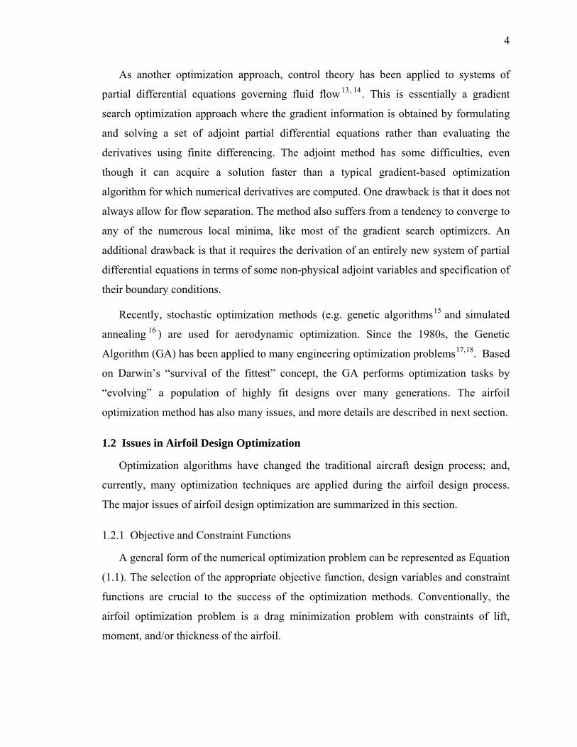
Discrete approach
The discrete approach uses the coordinates of the geometry illustrated in Figure 1.1 as
design variables. This approach is easy to implement, but the geometry changes are
limited by the number of design variables. It is difficult to maintain a smooth geometry
with a small number of design variables. Thus, the optimization solution may be
impractical to achieve.
Figure 1.1 Discrete approach using airfoil coordinates
Polynomial and spline approach
Using polynomial and spline representations for shape parameterization can reduce
the total number of design variables. A polynomial can describe a curve in a very
compact form with a small set of design variables. As an example, a curve can be
described as the polynomial shown in Equation (1.3)
∑−
=
=1
0
)(n
i
iiucuF (1.3)
Where n is the number of design variables, and u is the parameter coordinate along the
curve. The ic is a set of coefficient vectors corresponding to coordinates and the
components of these vectors can be used as design variables. The Bezier representation is
another mathematical form for representing curves.
∑−
=
=1
0, )()(
n
ipii uBpuF (1.4)
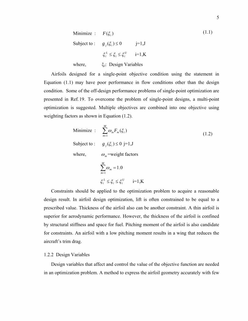
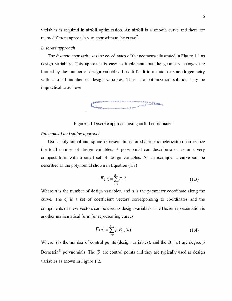
Where n is the number of control points (design variables), and the )(, uB pi are degree p
Bernstein21 polynomials. The ip are control points and they are typically used as design
variables as shown in Figure 1.2.
7
Figure 1.2 Bezier approach using control points
The Bezier form is an effective and accurate representation for shape optimization of
simple curves. However, complex curves require a high-degree Bezier form. As the
degree of a Bezier curve increases, so does the round-off error. Also, it is very inefficient
to compute a high-degree Bezier curve. A B-spline uses several low-degree Bezier
segments to cover the entire curve resulting in one composite curve. A multisegmented
B-spline curve can be described by
∑−
=
=1
0, )()(
n
ipii uNpuF (1.5)
Where ip are the B-spline control points, p is the degree, and )(, uN pi is the i-th B-spline
basis function of degree p. The drawback of the regular B-spline representation is its
inability to represent implicit conic sections accurately. However, a special form of B-
spline, nonuniform rational B-spline (NURBS) can represent quadric primitives as well
as free-form geometry. A NURBS curve is defined as
∑
∑
=
== n
iipi
n
iiipi
WuN
pWuNuR
1,
1,
)(
)()( (1.6)
Where the ip are the control points, iW are the weights, and the piN , are degree p B-spline
basis functions. Despite recent progress, it is still difficult to parameterize complex
shapes using polynomial and spline representations. This approach requires a large
number of control points, and optimization is prone to creating irregular or wavy
geometry with the spline representation.
Analytical approach (shape functions)
8
Hicks and Henne22 introduced a compact formulation for parameterization of airfoils.
The formulation is based on linearly adding shape functions to a baseline shape. The
contribution of each parameter is determined by the value of the participating coefficient
(which may be used as a design variable) associated with that function. The y-coordinates
of an airfoil can be expressed by Equation (1.7). The optimum geometry and the
efficiency of the design method may rely on the selection of the shape functions and the
number of shape functions used to represent the airfoil.
∑= )()( xfxy iiξ
(ξi: Design Variables, fi: Shape Functions, x : x coordinates of curve)
(1.7)
Mathematically, any continuous function or curve defined on a closed interval can be
represented by an infinite series of normal mode functions that form a complete set of
bases. However, an infinite number of series is not needed if the approximate curve
represented by shape functions is within the limit of a required norm of error tolerance.
Base airfoils can be added to this representation of an airfoil as shown in (1.8).
Especially for gradient-based optimization methods, starting from a typical airfoil would
be a reasonable strategy for searching the optimum airfoil. This would be achieved by
setting the initial values of 0iξ = . For a non-gradient-based method, such as the GA
(Genetic Algorithm), including a base airfoil will increase the “smoothness” of airfoil
shapes with the same upper and lower bounds on the shape function multiplier design
variables.
∑ξ+= )()()( Airfoil Base xfxyxy ii
(ξi: Design Variables, fi: Shape Functions)
(1.8)
This method is very effective for wing parameterization, but it is difficult to
generalize it for a complex geometry and hard to find very different shapes (i.e. the
design space is limited to the perturbations from the base shape available from the
)(xfiiξ terms).
9
1.2.3 Global Optimization
Gradient-based optimization
In the early stages of the design process, the search for optimal airfoil shapes
encompasses a broad range of possibilities. If the aerodynamic design space is smooth
enough (e.g. continuous first derivatives), Gradient-based Methods (GM) usually have
performance advantages over their global optimization counterparts. However, the
aerodynamic performance of an airfoil is very sensitive to the surface geometry, and it is
difficult to guarantee the convexness or unimodality of the objective functions used in
airfoil optimization. Moreover, in transonic airfoil design, the drag objective function
itself may be discontinuous due to shock waves23. When a CFD solver is used as the
function evaluator, the iterative nature of CFD can also lead to small discontinuities of
the design space and “false minima” due to the solver convergence tolerance. One of the
well-known concerns of using gradient-based optimization techniques is that they
conclude their search at a point where some form of the Kuhn-Tucker conditions are
satisfied; however, these conditions only describe a local optimum point. For airfoil
design, this means that an airfoil shape found by a gradient-based optimizer is likely the
locally optimal solution nearest to the initial airfoil shape.
Non gradient-based optimization
Recently, the Genetic Algorithm (GA) has emerged as a viable (although more
costly) alternative for airfoil optimization24, 25, 26 because of its global search nature. A
GA has the ability to search highly multimodal, discontinuous design spaces. The GA
also locates designs at, or near, the global optimum without requiring an initial design
point. If numerous local optimum points exist in the airfoil design space, global
optimization techniques will be an appropriate way to design airfoils despite the penalty
of computational time increases. Furthermore, parallel and/or distributed computing can
mitigate some of the computational expense associated with the GA.
1.2.4 Flow Models
The optimization algorithm requires a function evaluator, and the accuracy of the
function evaluator affects the reliability and validity of the optimum solution.
10
Computational Fluid Dynamics (CFD) algorithms have been developed for the past two
decades and are considered an important tool for aerodynamic design 27 . With the
development of CFD, the optimization method is combined with CFD and used as a
design method.
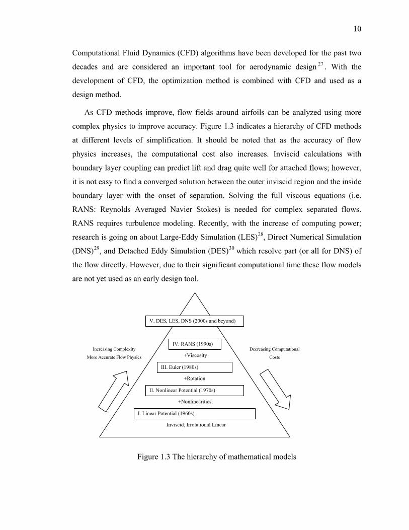
As CFD methods improve, flow fields around airfoils can be analyzed using more
complex physics to improve accuracy. Figure 1.3 indicates a hierarchy of CFD methods
at different levels of simplification. It should be noted that as the accuracy of flow
physics increases, the computational cost also increases. Inviscid calculations with
boundary layer coupling can predict lift and drag quite well for attached flows; however,
it is not easy to find a converged solution between the outer inviscid region and the inside
boundary layer with the onset of separation. Solving the full viscous equations (i.e.
RANS: Reynolds Averaged Navier Stokes) is needed for complex separated flows.
RANS requires turbulence modeling. Recently, with the increase of computing power;
research is going on about Large-Eddy Simulation (LES)28, Direct Numerical Simulation
(DNS)29, and Detached Eddy Simulation (DES)30 which resolve part (or all for DNS) of
the flow directly. However, due to their significant computational time these flow models
are not yet used as an early design tool.
Figure 1.3 The hierarchy of mathematical models
+Turbulence
I. Linear Potential (1960s)
II. Nonlinear Potential (1970s)
III. Euler (1980s)
Inviscid, Irrotational Linear
+Nonlinearities
+Rotation
+Viscosity Decreasing Computational
Costs
V. DES, LES, DNS (2000s and beyond)
Increasing Complexity
More Accurate Flow Physics
IV. RANS (1990s)
11
Several airfoil design methods are reviewed in this section. With the increase of
computer power and the development of numerical methods, the optimization approach is
widely used for designing airfoil and aircraft. Optimization would provide innovative
design and a logical, systematic, decision process. However, optimization is still
computationally expensive when using CFD for analysis.
1.3 Morphing Aircraft
Significant research has been carried out to understand how birds fly to gain
inspiration for improved man-made aircraft31. Birds can morph their wing shape to attain
maneuverability and maximum performance in different flight conditions. Recent
enhancement of materials and actuation technology has encouraged the concept of a
Morphing Aircraft. Morphing aircraft and related programs are briefly introduced in this
section to provide research motivations.
1.3.1 Return to the First Flight
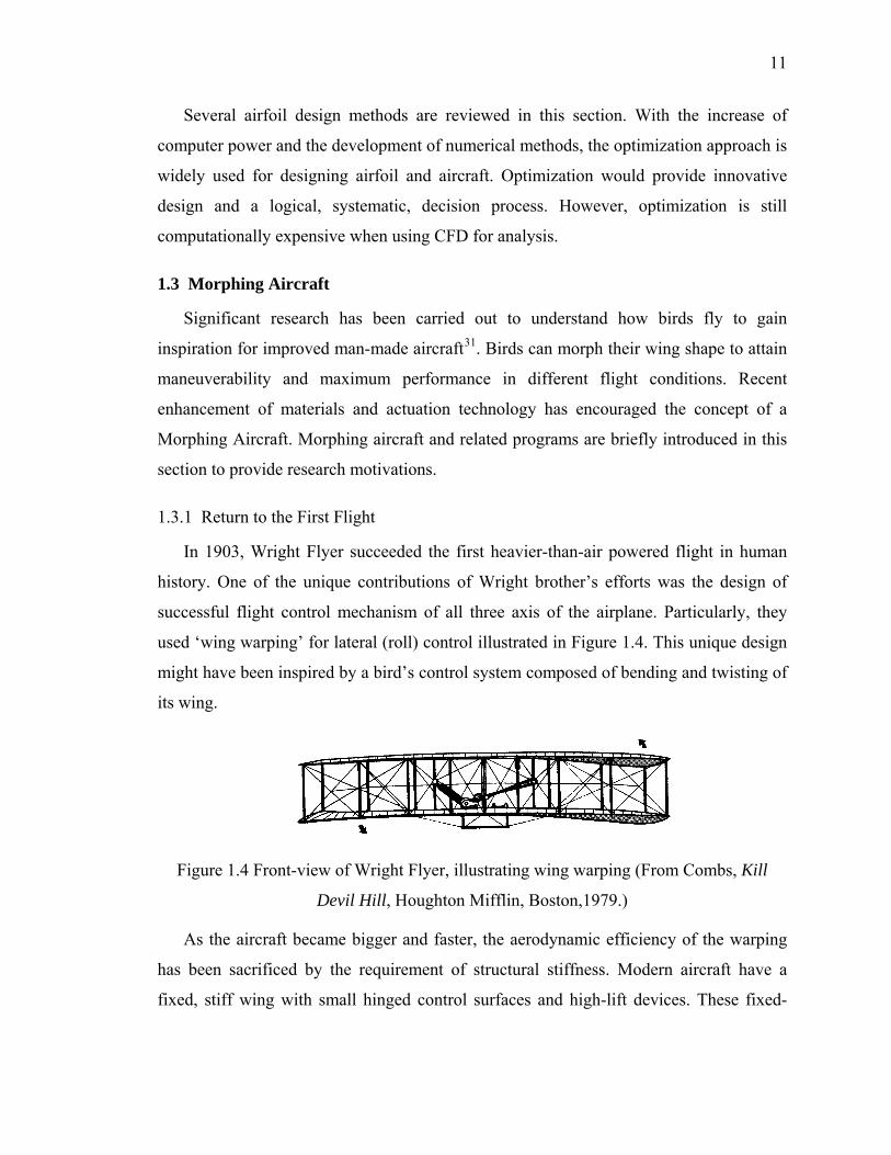
In 1903, Wright Flyer succeeded the first heavier-than-air powered flight in human
history. One of the unique contributions of Wright brother’s efforts was the design of
successful flight control mechanism of all three axis of the airplane. Particularly, they
used ‘wing warping’ for lateral (roll) control illustrated in Figure 1.4. This unique design
might have been inspired by a bird’s control system composed of bending and twisting of
its wing.
Figure 1.4 Front-view of Wright Flyer, illustrating wing warping (From Combs, Kill
Devil Hill, Houghton Mifflin, Boston,1979.)
As the aircraft became bigger and faster, the aerodynamic efficiency of the warping
has been sacrificed by the requirement of structural stiffness. Modern aircraft have a
fixed, stiff wing with small hinged control surfaces and high-lift devices. These fixed-
12
geometry wings are often designed for one mission capability or are designed as a
compromise among several capabilities. Also, discrete control surfaces deteriorate
aerodynamic efficiency by adding leakage and protuberance drag. Recently developed
smart material techniques can change the shape of the aircraft while maintaining stiffness.
This advancement turns our eye back on the first flying machine and draws our attention
to the design of a single aircraft that has multi-mission capability and aerodynamic
efficiency through morphing of the wing.
1.3.2 Definition of Morphing Aircraft
Usually, the word ‘morphing’ means substantial shape change or transfiguration. In
the context of NASA’s research on future flight vehicles31, morphing is defined as
‘efficient, multi-point adaptability’. Efficiency implies mechanical simplicity and system
weight reduction. Multi-point denotes accommodating diverse mission scenarios, and
adaptability means extensive versatility and resilience.
A Purdue research group defined the morphing aircraft as ‘A multi-role aircraft that,
through the use of “morphing technologies” (e.g. innovative actuators, effectors,
mechanisms), can change its shape to perform each of several dissimilar mission roles as
though the aircraft had been designed for each specific role’32.
Current conventional aircraft also reduce the penalties of single shape design through
the deflection of typical leading and trailing edge hinged control surfaces and high lift
devices. However, these hinged and discrete systems are highly complicated mechanical
devices with reliability problems and have gaps and external mechanisms that induce a
drag increase. A morphing aircraft may use smooth, deformable leading and trailing
edges, or possibly fully deformable airfoil sections instead of conventional discrete
movable surfaces.
1.3.3 Morphing Aircraft Related Programs
Mission Adaptive Wing (MAW) program
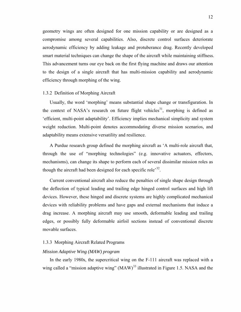
In the early 1980s, the supercritical wing on the F-111 aircraft was replaced with a
wing called a “mission adaptive wing” (MAW)33 illustrated in Figure 1.5. NASA and the
13
US Air Force launched a joint program called Advanced Fighter Technology Integration
(AFTI).
Figure 1.5 MAW modifications to F-111 (From NASA TM-4606)
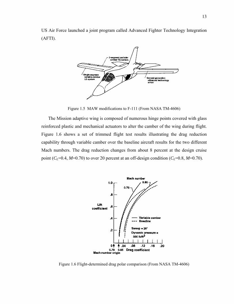
The Mission adaptive wing is composed of numerous hinge points covered with glass
reinforced plastic and mechanical actuators to alter the camber of the wing during flight.
Figure 1.6 shows a set of trimmed flight test results illustrating the drag reduction
capability through variable camber over the baseline aircraft results for the two different
Mach numbers. The drag reduction changes from about 8 percent at the design cruise
point (CL=0.4, M=0.70) to over 20 percent at an off-design condition (CL=0.8, M=0.70).
Figure 1.6 Flight-determined drag polar comparison (From NASA TM-4606)
14
Although the successful flight test of the MAW F-111 proved the benefits of variable
camber, the wing was generally considered too heavy and complex for practical
applications. The challenge was to find a way to easily bend a wing that is stiff and strong
enough to sustain the high loads of an aircraft in flight, with motors small enough to fit
inside its narrow space.
Smart Wing program
DARPA (Defense Advanced Research Projects Agency) initiated the Smart Wing
program34 in 1995 to incorporate the benefits of variable camber of MAW and variable
wing twist of Active Aeroelatic Wing (AAW). The overall objective of the Smart Wing
program was to develop smart technologies and demonstrate novel actuation systems to
improve the aerodynamic and aeroelastic performance of military aircraft. Many
researchers have investigated the use of fully integrated adaptive material actuator
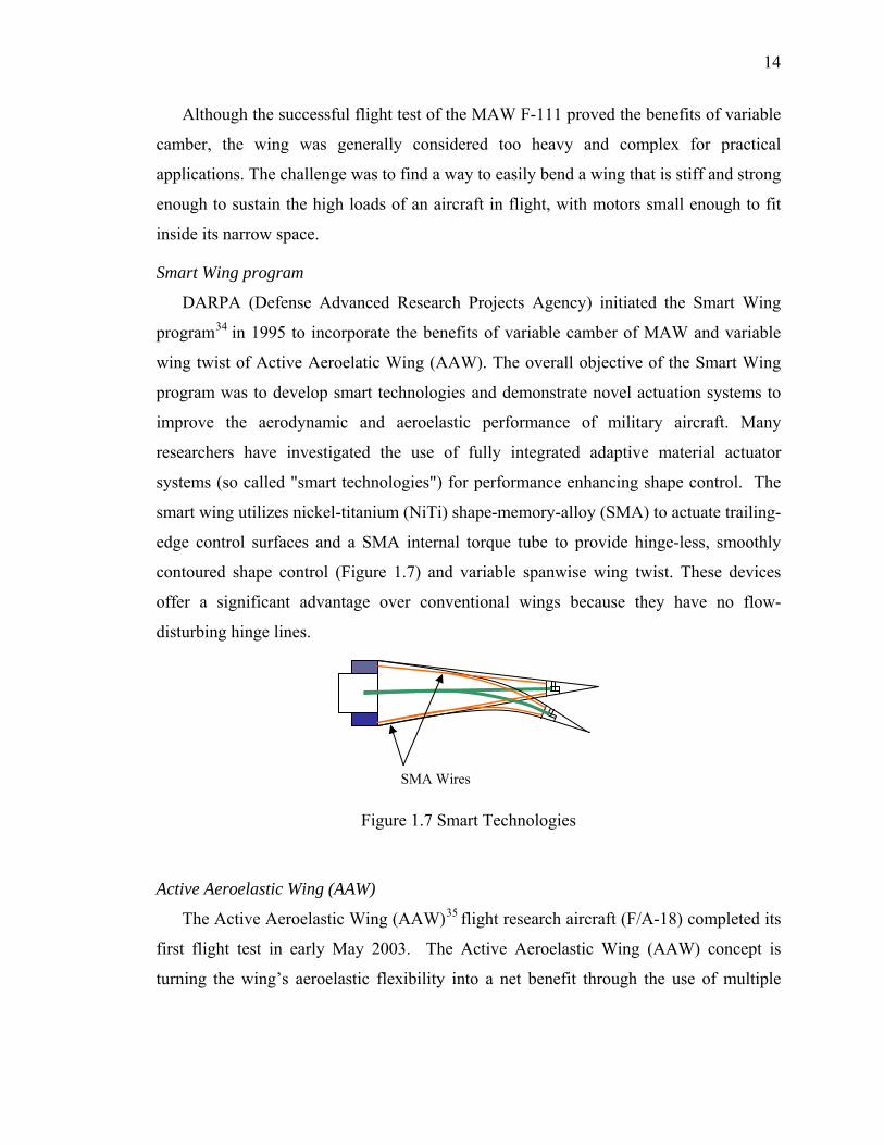
systems (so called "smart technologies") for performance enhancing shape control. The
smart wing utilizes nickel-titanium (NiTi) shape-memory-alloy (SMA) to actuate trailing-
edge control surfaces and a SMA internal torque tube to provide hinge-less, smoothly
contoured shape control (Figure 1.7) and variable spanwise wing twist. These devices
offer a significant advantage over conventional wings because they have no flow-
disturbing hinge lines.
Figure 1.7 Smart Technologies
Active Aeroelastic Wing (AAW)
The Active Aeroelastic Wing (AAW)35 flight research aircraft (F/A-18) completed its
first flight test in early May 2003. The Active Aeroelastic Wing (AAW) concept is
turning the wing’s aeroelastic flexibility into a net benefit through the use of multiple
SMA Wires
15
leading and trailing edge control surfaces activated by a digital flight control system.
AAW utilizes the energy of the air stream to achieve the desired wing twist with very
little control surface motion. The wing then creates the needed control forces with less
effort than an inflexible wing. At higher dynamic pressures, the AAW control surfaces
are used as "tabs" that promote wing twist for added control force capability instead of
trying to overcome control surface losses due to wing elastic twist. At these high dynamic
pressures, large amounts of control power can be generated using the control surfaces to
twist the wing. In the same design, the AAW control can also minimize drag at low wing
strain conditions and minimize structural loads at high wing strain conditions.
NASA’s Morphing Aircraft program
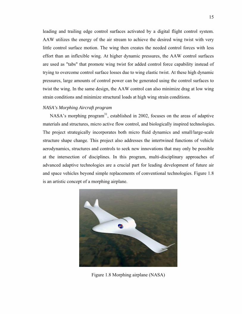
NASA’s morphing program31, established in 2002, focuses on the areas of adaptive
materials and structures, micro active flow control, and biologically inspired technologies.
The project strategically incorporates both micro fluid dynamics and small/large-scale
structure shape change. This project also addresses the intertwined functions of vehicle
aerodynamics, structures and controls to seek new innovations that may only be possible
at the intersection of disciplines. In this program, multi-disciplinary approaches of
advanced adaptive technologies are a crucial part for leading development of future air
and space vehicles beyond simple replacements of conventional technologies. Figure 1.8
is an artistic concept of a morphing airplane.
Figure 1.8 Morphing airplane (NASA)
16
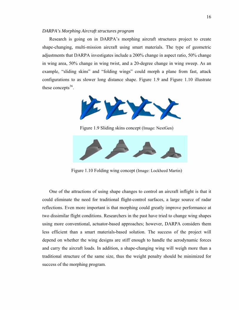
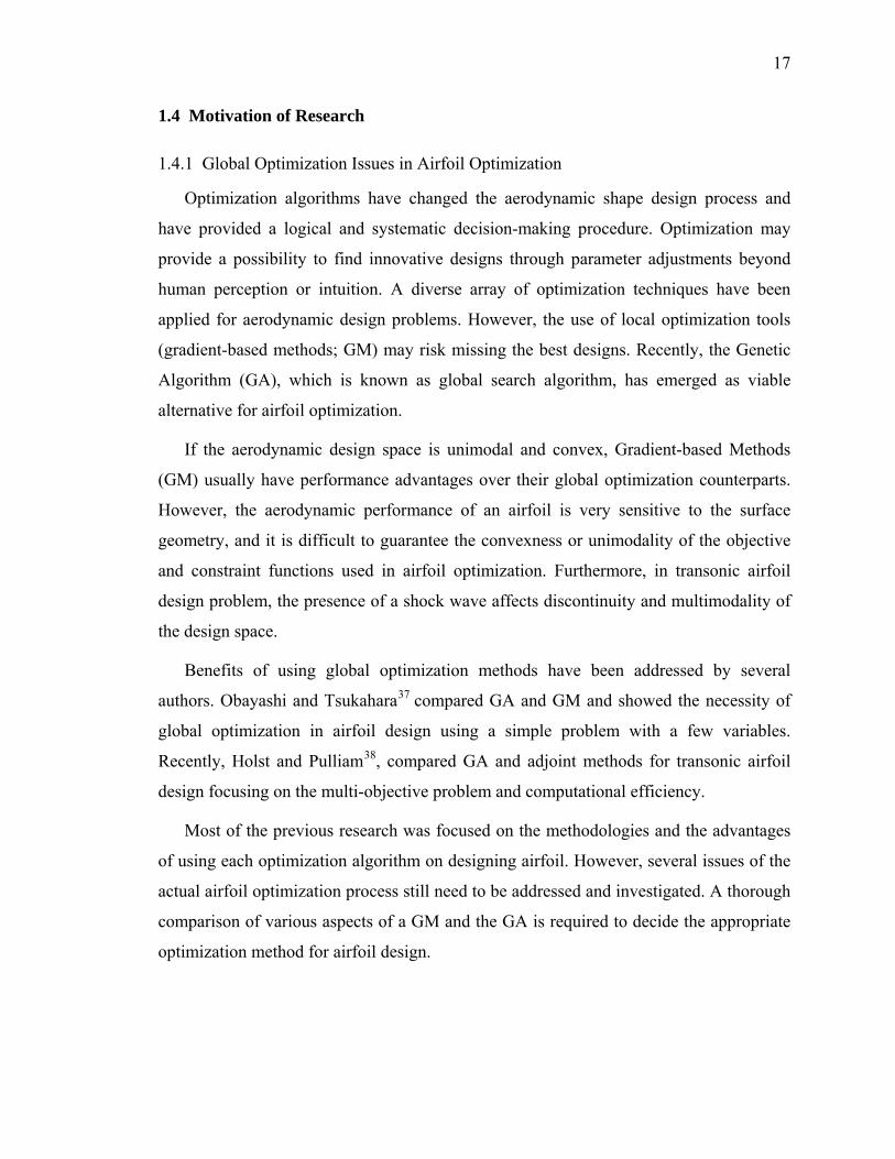
DARPA’s Morphing Aircraft structures program
Research is going on in DARPA’s morphing aircraft structures project to create
shape-changing, multi-mission aircraft using smart materials. The type of geometric
adjustments that DARPA investigates include a 200% change in aspect ratio, 50% change
in wing area, 50% change in wing twist, and a 20-degree change in wing sweep. As an
example, “sliding skins” and “folding wings” could morph a plane from fast, attack
configurations to as slower long distance shape. Figure 1.9 and Figure 1.10 illustrate
these concepts36.
Figure 1.9 Sliding skins concept (Image: NextGen)
Figure 1.10 Folding wing concept (Image: Lockheed Martin)
One of the attractions of using shape changes to control an aircraft inflight is that it
could eliminate the need for traditional flight-control surfaces, a large source of radar
reflections. Even more important is that morphing could greatly improve performance at
two dissimilar flight conditions. Researchers in the past have tried to change wing shapes
using more conventional, actuator-based approaches; however, DARPA considers them
less efficient than a smart materials-based solution. The success of the project will
depend on whether the wing designs are stiff enough to handle the aerodynamic forces
and carry the aircraft loads. In addition, a shape-changing wing will weigh more than a
traditional structure of the same size, thus the weight penalty should be minimized for
success of the morphing program.
17
1.4 Motivation of Research
1.4.1 Global Optimization Issues in Airfoil Optimization
Optimization algorithms have changed the aerodynamic shape design process and
have provided a logical and systematic decision-making procedure. Optimization may
provide a possibility to find innovative designs through parameter adjustments beyond
human perception or intuition. A diverse array of optimization techniques have been
applied for aerodynamic design problems. However, the use of local optimization tools
(gradient-based methods; GM) may risk missing the best designs. Recently, the Genetic
Algorithm (GA), which is known as global search algorithm, has emerged as viable
alternative for airfoil optimization.
If the aerodynamic design space is unimodal and convex, Gradient-based Methods
(GM) usually have performance advantages over their global optimization counterparts.
However, the aerodynamic performance of an airfoil is very sensitive to the surface
geometry, and it is difficult to guarantee the convexness or unimodality of the objective
and constraint functions used in airfoil optimization. Furthermore, in transonic airfoil
design problem, the presence of a shock wave affects discontinuity and multimodality of
the design space.
Benefits of using global optimization methods have been addressed by several
authors. Obayashi and Tsukahara37 compared GA and GM and showed the necessity of
global optimization in airfoil design using a simple problem with a few variables.
Recently, Holst and Pulliam38, compared GA and adjoint methods for transonic airfoil
design focusing on the multi-objective problem and computational efficiency.
Most of the previous research was focused on the methodologies and the advantages
of using each optimization algorithm on designing airfoil. However, several issues of the
actual airfoil optimization process still need to be addressed and investigated. A thorough
comparison of various aspects of a GM and the GA is required to decide the appropriate
optimization method for airfoil design.
18
1.4.2 Morphing Airfoil Design
Recently, a deformable wing concept was introduced as a future aircraft technology.
A newly introduced morphing aircraft can change its wing freely like a bird. Most of the
previous morphing aircraft related research was focused on device development for
changing the shape of the aircraft. However, a system level approach on the overall
performance of morphing aircraft including vehicle weight, size, cost has not been
investigated as much.
The concept of morphing aircraft has generated a new design goal for aerodynamic
configuration design and optimization area. Most aircraft wings are designed as a single
shape resulting in a compromise of performance at several design conditions. A single
point design will have performance penalties at flight conditions other than the design
condition. Generally, a multi-point problem formulation is used for airfoil or wing design.
The multi-point optimization includes tradeoffs between the multiple design objectives.
In the case of a morphing aircraft, the design objective is no longer a single aerodynamic
objective as in the conventional aerodynamic shape optimization. It does not require
aerodynamic tradeoffs between multiple design objectives. The morphing aircraft can
adjust the wing shape to the optimal shape for any flight condition encountered by the
aircraft. This adaptation will improve the aerodynamic performance of the aircraft.
However, morphing aircraft requires an extra mechanism to change the wing shape.
Therefore, to account for the total performance benefits of morphing aircraft, a new
design strategy is needed to embrace the variation of the wing shape in the optimization
process that addresses the effort needed to morph the shape of the airfoil.
Another issue of morphing aircraft optimization is how to model the morphing cost.
In previous research, Prock39 et al suggested using a simple strain energy model for
morphing aircraft design. This model is based on the assumption that the strain energy
stored in the wing will be similar to the energy required for the actuator. Also, it is
assumed that the actuator energy will be proportional to the morphing cost. This simple
spring actuation model, however, neglected the effect of aerodynamic load. In real flight
conditions, the effect of aerodynamic force cannot be neglected. If the stiffness of the
wing is very high, the strain energy will be enough to account for the actuation energy.
19
However, if the stiffness decreases, which is required for morphing aircraft, the
aerodynamic force is relatively more important and needs to be included in the actuation
energy model.
1.5 Thesis Objectives
The first objective of this research is to investigate the issues associated with using a
global search for transonic airfoil design by comparing the Genetic Algorithm (GA) with
a Gradient-based optimization method (GM). The issues to be addressed in this transonic
airfoil design study will include selecting design variables and their boundaries, trimming,
computational cost, existence of local optima, CFD grid selection and choosing the base
airfoil.
The second objective is to develop a design process and strategy that incorporates
morphing cost in the design of morphing airfoils, based on the method developed through
the transonic airfoil optimization. The resulting airfoil set should provide the desired
aerodynamic performance and also satisfy multiple missions with the smallest actuation
energy (morphing cost). This will show the tradeoffs between improved performance and
actuation energy.
The third objective is to improve the accuracy of the morphing energy model by
incorporating an aerodynamic load model. The suggested actuation model (morphing cost
model) with an aerodynamic load term would be more realistic compared to the simple
strain energy model.
1.6 Thesis Organization
In Chapter 2, most of the optimization issues discussed in section 1.2 are addressed
for the transonic airfoil optimization problem and the development of the transonic airfoil
optimization process is covered. Chapter 3 focuses on formulating a new objective
function for morphing aircraft optimization. The airfoil optimization strategies developed
in Chapter 2 are employed. Chapter 4 discusses the actuation energy modeling for the
morphing aircraft. Aerodynamic work is modeled and added to the simple strain energy

20
model used in Chapter3. Finally, Chapter 5 summarizes the work with concluding
remarks and future directions.
21
CHAPTER 2 TRANSONIC AIRFOIL OPTIMIZATION
To investigate the issues in airfoil optimization, drag minimization problem in the
transonic regime is selected as a test case. Transonic airflows present some of the most
complex challenges in aerodynamics because of the air behavior as it transitions from
subsonic to supersonic speeds. The feasible direction method (CONMIN module) and
Genetic Algorithm (GA) were selected as optimization algorithm.
In transonic flow, the major source of the drag is the ‘wave drag’ due to the shock
wave. Thus, it is expected that the gradient-based method will stop at the first shock free
conditions. However, the shock wave is not the only source of the drag in transonic flow.
Many different shock-free airfoils creating a several local minima may exist. This can be
tested by comparing the gradient based optimization results started from several different
initial points, and this will be shown in this chapter.
Because of the expected multimodal design space, a global optimization method
seems more appropriate for the transonic airfoil optimization problem. An accurate flow
solver, enough to resolve all the drag components, is needed to investigate the transonic
airfoil optimization problem, which will increase the computational time dramatically for
a global optimization technique.
Computational cost is a primary issue for the GA to be considered as an alternative to
a gradient-based method. Fortunately, the nature of the GA algorithm is well suited to
parallel processing and could reduce GA’s computational cost to an affordable level. The
parallelization issue of the GA is also presented in this chapter.
22
The detailed process of designing the minimum drag airfoil using the GA and GM
and the results comparisons between these two methods are presented to help to identify
the issues.
2.1 Design Variables
An airfoil shape can be regarded as a curve and there are many ways to parameterize
a curve. The intend is to represent the airfoil with a small number of variables with
certain accuracy and maintaining reasonable shapes during the search. Samareh 40
surveyed shape parameterization techniques and compared the pros and cons of each
method. However, there are no clear guidelines to select one most efficient
parameterization method.
The shape representation is especially important for global optimization. A large
number of design variables can increase computational cost. Also, during a global search,
a wide range of variable values may be investigated. If combinations of variables happen
to represent an unrealistic airfoil, e.g. with upper and lower surfaces crossed, the global
search method may likely encounter this combination.
To choose an appropriate shape representation and set of design variables, a simple
reconstruction test is performed. The reconstructed shape is acquired by the least-square
solution of the difference between the original airfoil shape and the regenerated airfoil
shape.
Two parameterization methods are tested. One is the analytical approach41 that uses
shape functions added to a base airfoil shape and the other is the spline40 approach. For
the analytical approach, the y-coordinate positions are represented by Equation (2.1).
Three different shape functions (modified Hicks-Henne41, NACA normal mode 42 and
Wagner functions43) are selected for this test, and the NACA0012 airfoil is used as the
base airfoil. As the design variables iξ vary from zero, the represented airfoil shape
varies from the base airfoil shape.
23
∑+= )()(),( Airfoil Base xfxyxy iii ξξ
(ξi: Design Variables, fi: Shape Functions)
(2.1)
A Bezier curve44, described in Equation (2.2), is tested as an example of a spline
approach, where the design variables are multiplied by a polynomial function. There is no
base airfoil in this case.
∑= )(),( , xBxy piii ξξ
(ξi: Design Variables, Bi,p: degree P Bernstein polynomials )
(2.2)
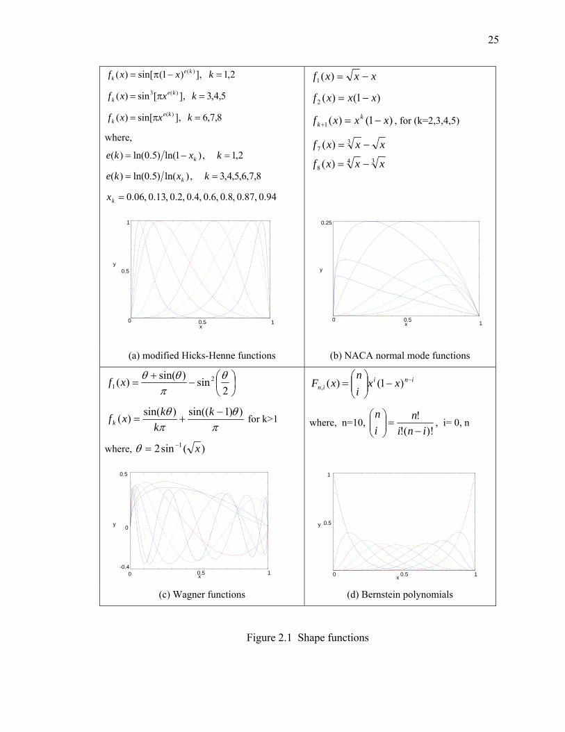
All shape functions used in this thesis and Bernstein polynomials are shown in Figure
2.1. For the investigation of shape representations, the Whitcomb supercritical airfoil45
are selected as a target airfoils; the NACA0012 is used as the base airfoil (as mentioned
above). Approximate sets of y-coordinates were regenerated by the solution design
variables ξ ′ that minimize (yactual – y(ξi)) at several ordinate(x) locations on the airfoil.
The least square solution is shown in Equation (2.3).
bAAA TTi
1)( −=′ξ
(b: y coordinate of target airfoil, A: matrix composed of x ordinate of each
shape functions)
(2.3)
A total of 16 design variables (8 variables for each surface) are used in this test. The
norm of the error was compared in Table 2.1, and the shape difference is compared in
Figure 2.2. Table 2.1 shows that the analytical method with the modified Hicks-Henne
functions has the best reconstruction capability for both the upper and lower surfaces.
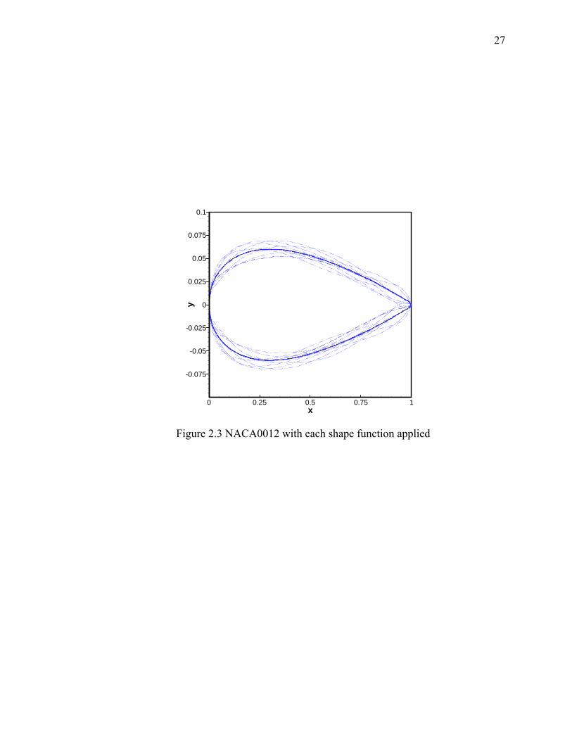
In this research, the analytical method with modified Hicks-Henne functions is
chosen for representing airfoils. The design variables are multipliers that determine the
magnitude of the shape function as it is added to the baseline shape. Figure 2.1 depicts
the shape functions and Figure 2.3 shows their individual effects on a baseline NACA
0012 airfoil when one of the ξ values is 0.015.
24
Table 2.1 Error norm comparison (Target airfoil: Whitcomb supercritical airfoil)
Modified Hicks-Henne functions
NACA Normal Mode functions
Wagner Functions Bezier Curve
Upper surface
2estimateoriginal yy −
0.00200
0.00088
0.00130
0.01680
Lower surface
2estimateoriginal yy −
0.00330
0.00510
0.00440
0.01620
25
Figure 2.1 Shape functions
2,1 ],)1(sin[)( )( =−π= kxxf kek
5,4,3 ],[sin)( )(3 =π= kxxf kek
8,7,6 ],sin[)( )( =π= kxxf kek
where,
2,1 ,)1ln()5.0ln()( =−= kxke k
8,7,6,5,4,3 ,)ln()5.0ln()( == kxke k
94.0 ,87.0 ,8.0 ,6.0 ,4.0 ,2.0 ,13.0 ,06.0=kx
xxxf −=)(1
)1()(2 xxxf −=
)1()(1 xxxf kk −=+ , for (k=2,3,4,5)
348
37
)(
)(
xxxf
xxxf
−=
−=
(a) modified Hicks-Henne functions (b) NACA normal mode functions
⎟⎠⎞
⎜⎝⎛−
+=
2sin)sin()( 2
1θ
πθθxf
πθ
πθ ))1sin(()sin()( −
+=k
kkxfk for k>1
where, )(sin2 1 x−=θ
iniin xx
in
xF −−⎟⎟⎠
⎞⎜⎜⎝
⎛= )1()(,
where, n=10, )!(!
!ini
nin
−=⎟⎟
⎠
⎞⎜⎜⎝
⎛, i= 0, n
(c) Wagner functions (d) Bernstein polynomials
1 0 0.5
0.25
x
y
0.5 1 0
0.5
1
x
y
0 0.5 1 -0.4
0
0.5
x
y
0 0.5 1
0.5
1
x
y

26
0 0.2 0.4 0.6 0.8 1X
-0.06
-0.04
-0.02
0
0.02
0.04
0.06
Y
WhitcombReconstructed (Hicks-Henne functions)
0 0.2 0.4 0.6 0.8 1X
-0.06
-0.04
-0.02
0
0.02
0.04
0.06
Y
WhitcombReconstructed (NACA mode functions)
(a) Hicks-Henne functions (b) NACA normal mode functions
0 0.2 0.4 0.6 0.8 1X
-0.06
-0.04
-0.02
0
0.02
0.04
0.06
Y
WhitcombReconstructed (Wagner functions)
0 0.2 0.4 0.6 0.8 1X
-0.06
-0.04
-0.02
0
0.02
0.04
0.06
Y
WhitcombReconstructed (Bezier functions)
(c) Wagner functions (d) Bezier curve
Figure 2.2 Original versus reconstructed airfoils
27
0 0.25 0.5 0.75 1x
-0.075
-0.05
-0.025
0
0.025
0.05
0.075
0.1
y
Figure 2.3 NACA0012 with each shape function applied
28
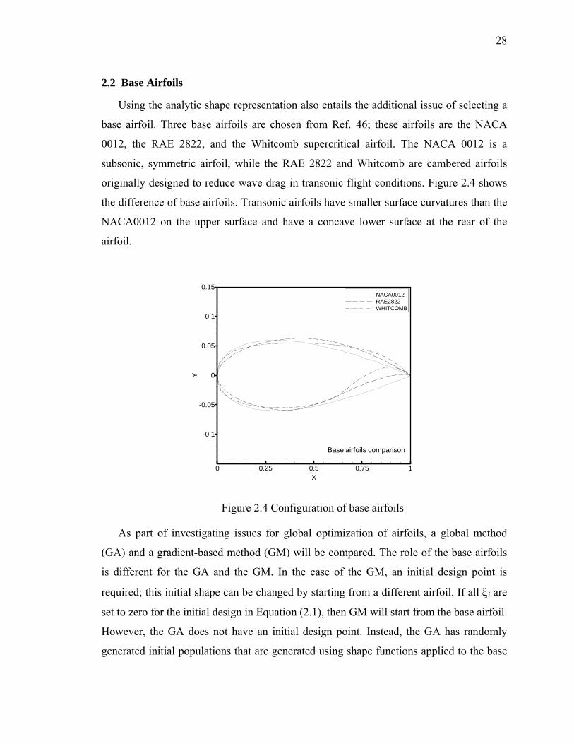
2.2 Base Airfoils
Using the analytic shape representation also entails the additional issue of selecting a
base airfoil. Three base airfoils are chosen from Ref. 46; these airfoils are the NACA
0012, the RAE 2822, and the Whitcomb supercritical airfoil. The NACA 0012 is a
subsonic, symmetric airfoil, while the RAE 2822 and Whitcomb are cambered airfoils
originally designed to reduce wave drag in transonic flight conditions. Figure 2.4 shows
the difference of base airfoils. Transonic airfoils have smaller surface curvatures than the
NACA0012 on the upper surface and have a concave lower surface at the rear of the
airfoil.
0 0.25 0.5 0.75 1X
-0.1
-0.05
0
0.05
0.1
0.15
Y
NACA0012RAE2822WHITCOMB
Base airfoils comparison
Figure 2.4 Configuration of base airfoils
As part of investigating issues for global optimization of airfoils, a global method
(GA) and a gradient-based method (GM) will be compared. The role of the base airfoils
is different for the GA and the GM. In the case of the GM, an initial design point is
required; this initial shape can be changed by starting from a different airfoil. If all ξi are
set to zero for the initial design in Equation (2.1), then GM will start from the base airfoil.
However, the GA does not have an initial design point. Instead, the GA has randomly
generated initial populations that are generated using shape functions applied to the base
29
airfoils. Therefore, through altering the base airfoils, the GA can have a different range of
design space (possible airfoil shapes) with the same values for the upper and lower
bounds on the design variables.
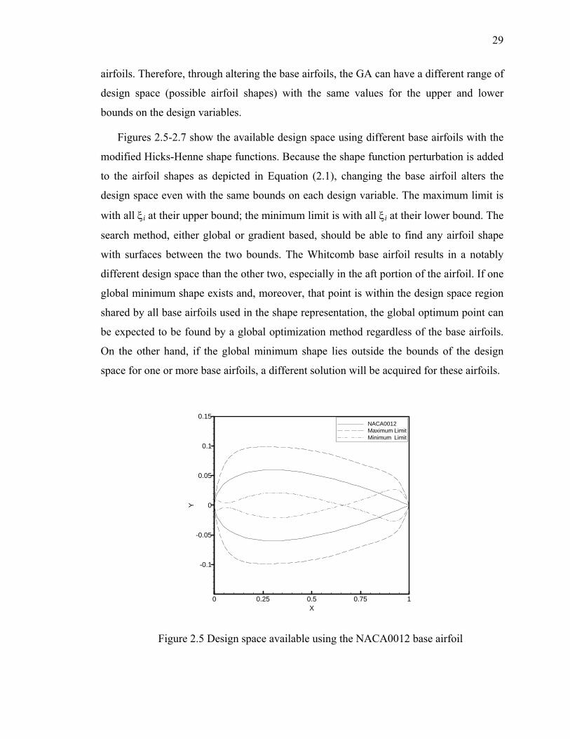
Figures 2.5-2.7 show the available design space using different base airfoils with the
modified Hicks-Henne shape functions. Because the shape function perturbation is added
to the airfoil shapes as depicted in Equation (2.1), changing the base airfoil alters the
design space even with the same bounds on each design variable. The maximum limit is
with all ξi at their upper bound; the minimum limit is with all ξi at their lower bound. The
search method, either global or gradient based, should be able to find any airfoil shape
with surfaces between the two bounds. The Whitcomb base airfoil results in a notably
different design space than the other two, especially in the aft portion of the airfoil. If one
global minimum shape exists and, moreover, that point is within the design space region
shared by all base airfoils used in the shape representation, the global optimum point can
be expected to be found by a global optimization method regardless of the base airfoils.
On the other hand, if the global minimum shape lies outside the bounds of the design
space for one or more base airfoils, a different solution will be acquired for these airfoils.
0 0.25 0.5 0.75 1X
-0.1
-0.05
0
0.05
0.1
0.15
Y
NACA0012Maximum LimitMinimum Limit
Figure 2.5 Design space available using the NACA0012 base airfoil
30
0 0.25 0.5 0.75 1X
-0.1
-0.05
0
0.05
0.1
0.15
Y
RAE2822Maximum LimitMinimum Limit
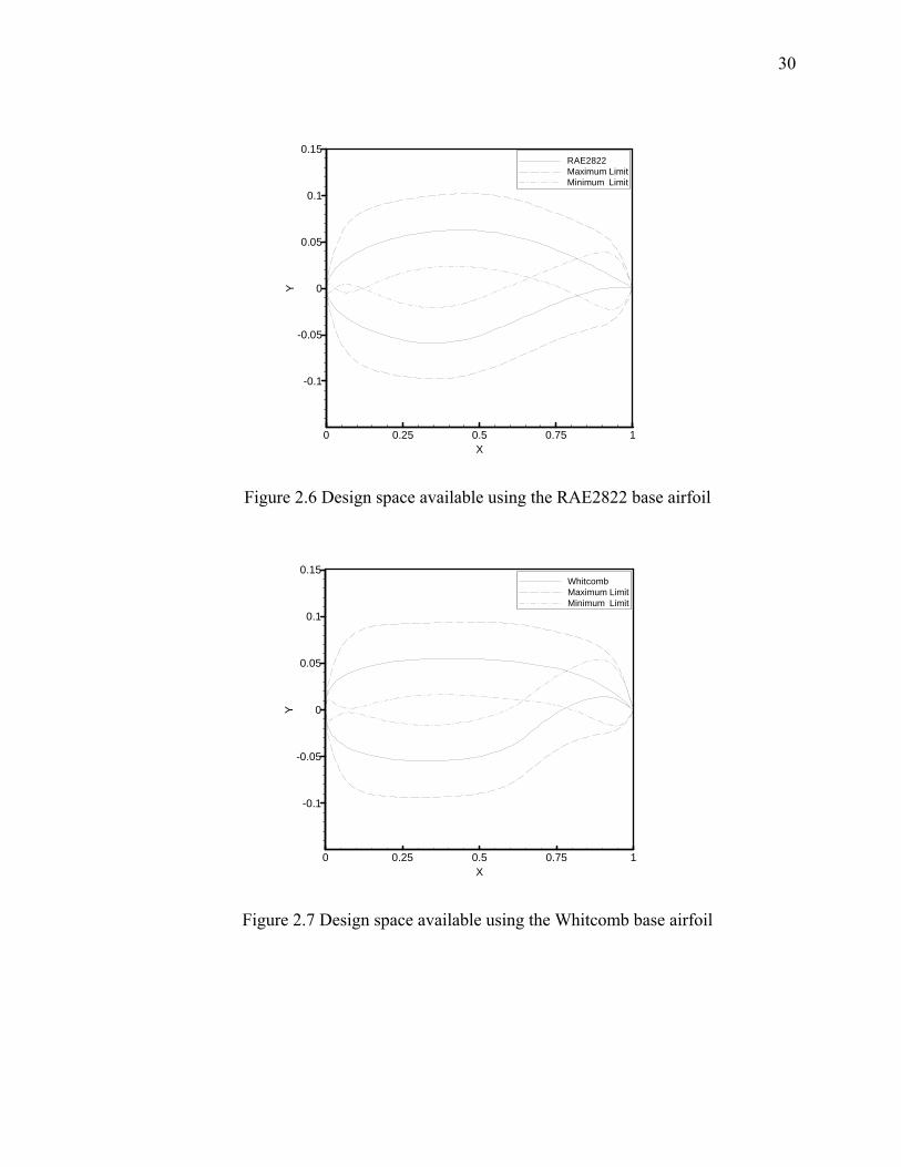
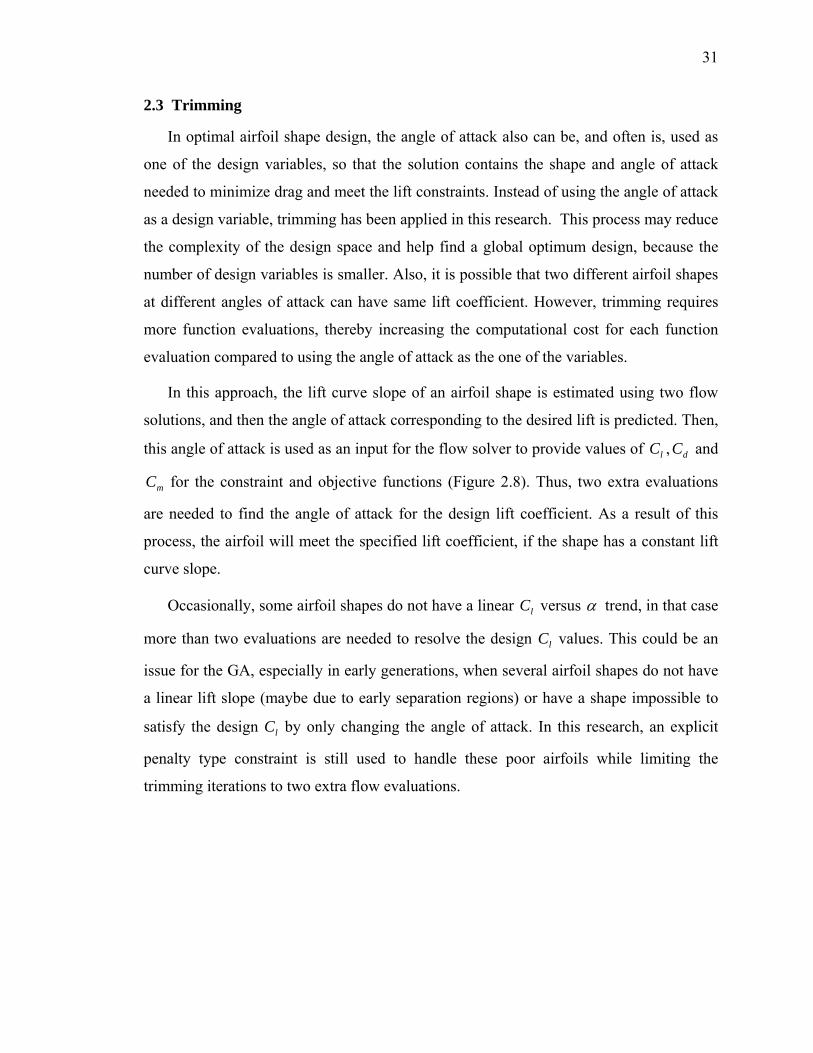
Figure 2.6 Design space available using the RAE2822 base airfoil
0 0.25 0.5 0.75 1X
-0.1
-0.05
0
0.05
0.1
0.15
Y
WhitcombMaximum LimitMinimum Limit
Figure 2.7 Design space available using the Whitcomb base airfoil
31
2.3 Trimming
In optimal airfoil shape design, the angle of attack also can be, and often is, used as
one of the design variables, so that the solution contains the shape and angle of attack
needed to minimize drag and meet the lift constraints. Instead of using the angle of attack
as a design variable, trimming has been applied in this research. This process may reduce
the complexity of the design space and help find a global optimum design, because the
number of design variables is smaller. Also, it is possible that two different airfoil shapes
at different angles of attack can have same lift coefficient. However, trimming requires
more function evaluations, thereby increasing the computational cost for each function
evaluation compared to using the angle of attack as the one of the variables.
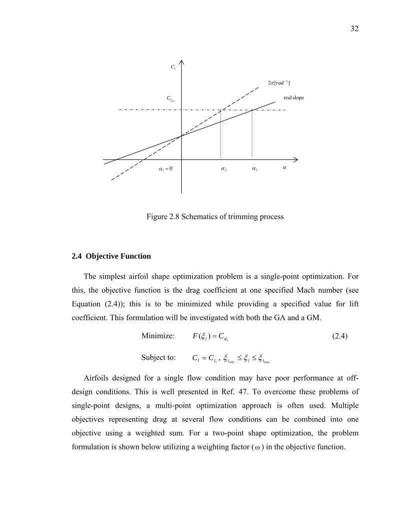
In this approach, the lift curve slope of an airfoil shape is estimated using two flow
solutions, and then the angle of attack corresponding to the desired lift is predicted. Then,
this angle of attack is used as an input for the flow solver to provide values of lC , dC and
mC for the constraint and objective functions (Figure 2.8). Thus, two extra evaluations
are needed to find the angle of attack for the design lift coefficient. As a result of this
process, the airfoil will meet the specified lift coefficient, if the shape has a constant lift
curve slope.
Occasionally, some airfoil shapes do not have a linear lC versus α trend, in that case
more than two evaluations are needed to resolve the design lC values. This could be an
issue for the GA, especially in early generations, when several airfoil shapes do not have
a linear lift slope (maybe due to early separation regions) or have a shape impossible to
satisfy the design lC by only changing the angle of attack. In this research, an explicit
penalty type constraint is still used to handle these poor airfoils while limiting the
trimming iterations to two extra flow evaluations.
32
Figure 2.8 Schematics of trimming process
2.4 Objective Function
The simplest airfoil shape optimization problem is a single-point optimization. For
this, the objective function is the drag coefficient at one specified Mach number (see
Equation (2.4)); this is to be minimized while providing a specified value for lift
coefficient. This formulation will be investigated with both the GA and a GM.
Minimize: 1
)( di CF =ξ
Subject to: 1ll CC = ,
maxmin iii ξξξ ≤≤
(2.4)
Airfoils designed for a single flow condition may have poor performance at off-
design conditions. This is well presented in Ref. 47. To overcome these problems of
single-point designs, a multi-point optimization approach is often used. Multiple
objectives representing drag at several flow conditions can be combined into one
objective using a weighted sum. For a two-point shape optimization, the problem
formulation is shown below utilizing a weighting factor ( ω ) in the objective function.
deslC
][2 1−radπ
slope real
lC
α01 =α 2α 3α
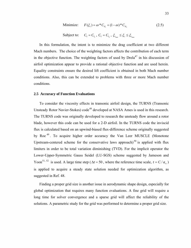
33
Minimize: 21
*)1(*)( ddi CCF ωωξ −+=
Subject to: 1ll CC = ,
2ll CC = , maxmin iii ξξξ ≤≤
(2.5)
In this formulation, the intent is to minimize the drag coefficient at two different
Mach numbers. The choice of the weighting factors affects the contribution of each term
in the objective function. The weighting factors of used by Drela47 in his discussion of
airfoil optimization appear to provide a rational objective function and are used herein.
Equality constraints ensure the desired lift coefficient is obtained in both Mach number
conditions. Also, this can be extended to problems with three or more Mach number
conditions.
2.5 Accuracy of Function Evaluations
To consider the viscosity effects in transonic airfoil design, the TURNS (Transonic
Unsteady Rotor Navier-Stokes) code48 developed at NASA Ames is used in this research.
The TURNS code was originally developed to research the unsteady flow around a rotor
blade, however this code can be used for a 2-D airfoil. In the TURNS code the inviscid
flux is calculated based on an upwind-biased flux-difference scheme originally suggested
by Roe 49 . To acquire higher order accuracy the Van Leer MUSCLE (Monotone
Upstream-centered scheme for the conservative laws approach)50 is applied with flux
limiters in order to be total variation diminishing (TVD). For the implicit operator the
Lower-Upper-Symmetric Gauss Seidel (LU-SGS) scheme suggested by Jameson and
Yoon51, 52 is used. A large time step ( 50=Δt , where the reference time scale, ∞= aCt / )
is applied to acquire a steady state solution needed for optimization algorithm, as
suggested in Ref. 48.
Finding a proper grid size is another issue in aerodynamic shape design, especially for
global optimization that requires many function evaluations. A fine grid will require a
long time for solver convergence and a sparse grid will affect the reliability of the
solutions. A parametric study for the grid was performed to determine a proper grid size.
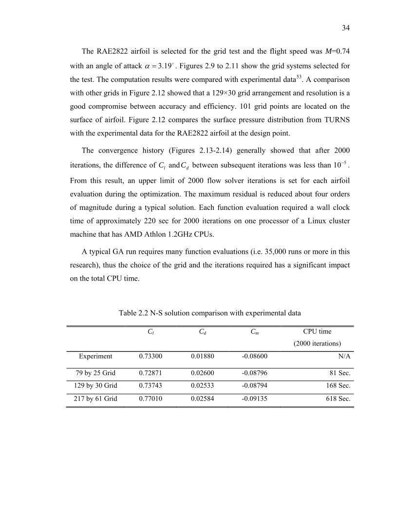
34
The RAE2822 airfoil is selected for the grid test and the flight speed was M=0.74
with an angle of attack 19.3=α . Figures 2.9 to 2.11 show the grid systems selected for
the test. The computation results were compared with experimental data53. A comparison
with other grids in Figure 2.12 showed that a 129×30 grid arrangement and resolution is a
good compromise between accuracy and efficiency. 101 grid points are located on the
surface of airfoil. Figure 2.12 compares the surface pressure distribution from TURNS
with the experimental data for the RAE2822 airfoil at the design point.
The convergence history (Figures 2.13-2.14) generally showed that after 2000
iterations, the difference of lC and dC between subsequent iterations was less than 510− .
From this result, an upper limit of 2000 flow solver iterations is set for each airfoil
evaluation during the optimization. The maximum residual is reduced about four orders
of magnitude during a typical solution. Each function evaluation required a wall clock
time of approximately 220 sec for 2000 iterations on one processor of a Linux cluster
machine that has AMD Athlon 1.2GHz CPUs.
A typical GA run requires many function evaluations (i.e. 35,000 runs or more in this
research), thus the choice of the grid and the iterations required has a significant impact
on the total CPU time.
Table 2.2 N-S solution comparison with experimental data
Cl Cd Cm CPU time
(2000 iterations)
Experiment 0.73300 0.01880 -0.08600 N/A
79 by 25 Grid 0.72871 0.02600 -0.08796 81 Sec.
129 by 30 Grid 0.73743 0.02533 -0.08794 168 Sec.
217 by 61 Grid 0.77010 0.02584 -0.09135 618 Sec.
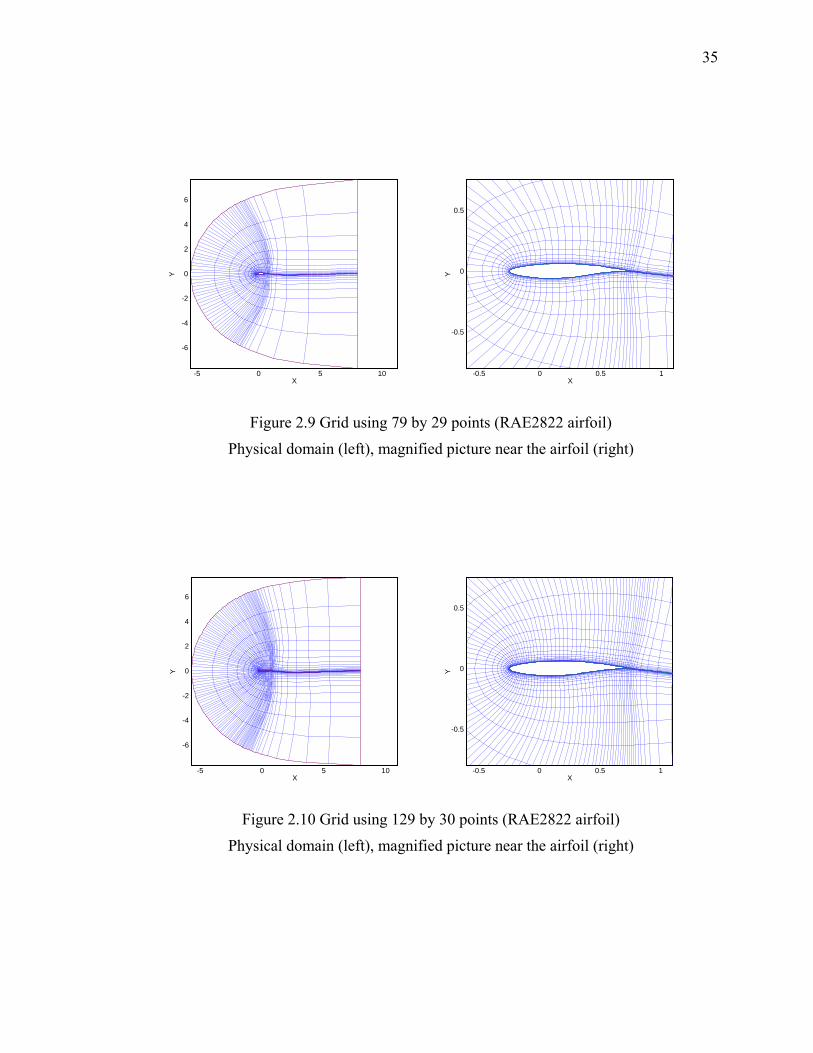
35
-5 0 5 10X
-6
-4
-2
0
2
4
6
Y
-0.5 0 0.5 1X
-0.5
0
0.5
Y
Figure 2.9 Grid using 79 by 29 points (RAE2822 airfoil)
Physical domain (left), magnified picture near the airfoil (right)
-5 0 5 10X
-6
-4
-2
0
2
4
6
Y
-0.5 0 0.5 1X
-0.5
0
0.5
Y
Figure 2.10 Grid using 129 by 30 points (RAE2822 airfoil)
Physical domain (left), magnified picture near the airfoil (right)
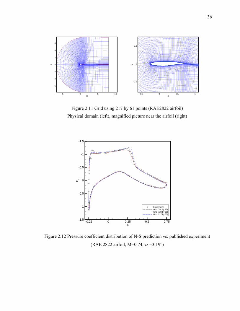
36
-5 0 5 10X
-6
-4
-2
0
2
4
6
Y
-0.5 0 0.5 1X
-0.5
0
0.5
Y
Figure 2.11 Grid using 217 by 61 points (RAE2822 airfoil)
Physical domain (left), magnified picture near the airfoil (right)
-0.25 0 0.25 0.5 0.75x
-1.5
-1
-0.5
0
0.5
1
1.5
Cp
ExperimentGrid (79 by 25)Grid (129 by 30)Grid (217 by 60)
Figure 2.12 Pressure coefficient distribution of N-S prediction vs. published experiment
(RAE 2822 airfoil, M=0.74, α =3.19°)
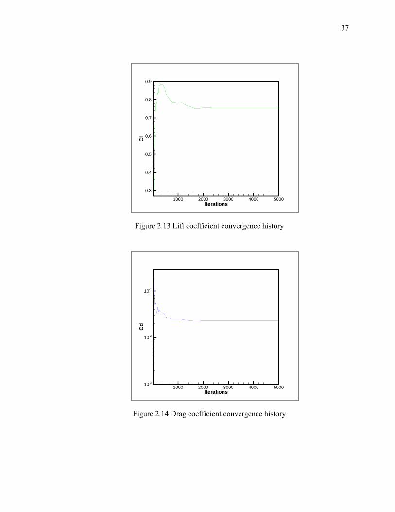
37
1000 2000 3000 4000 5000Iterations
0.3
0.4
0.5
0.6
0.7
0.8
0.9
Cl
Figure 2.13 Lift coefficient convergence history
1000 2000 3000 4000 5000Iterations
10-3
10-2
10-1
Cd
Figure 2.14 Drag coefficient convergence history
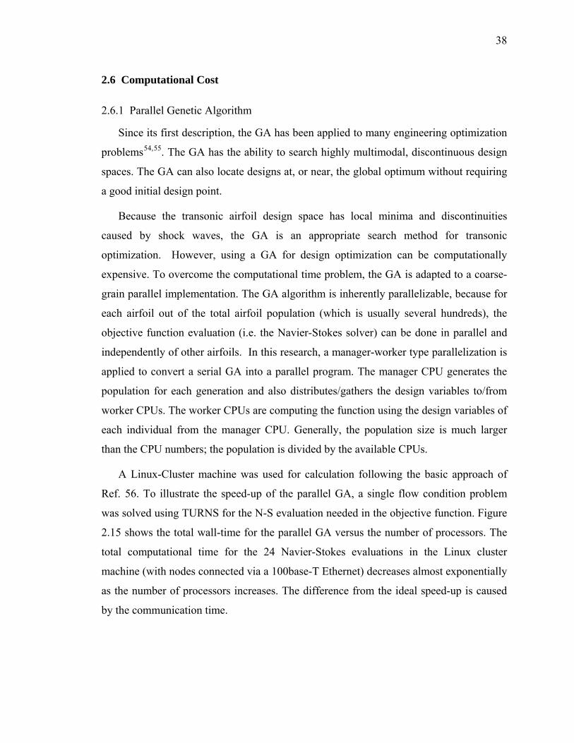
38
2.6 Computational Cost
2.6.1 Parallel Genetic Algorithm
Since its first description, the GA has been applied to many engineering optimization
problems54,55. The GA has the ability to search highly multimodal, discontinuous design
spaces. The GA can also locate designs at, or near, the global optimum without requiring
a good initial design point.
Because the transonic airfoil design space has local minima and discontinuities
caused by shock waves, the GA is an appropriate search method for transonic
optimization. However, using a GA for design optimization can be computationally
expensive. To overcome the computational time problem, the GA is adapted to a coarse-
grain parallel implementation. The GA algorithm is inherently parallelizable, because for
each airfoil out of the total airfoil population (which is usually several hundreds), the
objective function evaluation (i.e. the Navier-Stokes solver) can be done in parallel and
independently of other airfoils. In this research, a manager-worker type parallelization is
applied to convert a serial GA into a parallel program. The manager CPU generates the
population for each generation and also distributes/gathers the design variables to/from
worker CPUs. The worker CPUs are computing the function using the design variables of
each individual from the manager CPU. Generally, the population size is much larger
than the CPU numbers; the population is divided by the available CPUs.
A Linux-Cluster machine was used for calculation following the basic approach of
Ref. 56. To illustrate the speed-up of the parallel GA, a single flow condition problem
was solved using TURNS for the N-S evaluation needed in the objective function. Figure
2.15 shows the total wall-time for the parallel GA versus the number of processors. The
total computational time for the 24 Navier-Stokes evaluations in the Linux cluster
machine (with nodes connected via a 100base-T Ethernet) decreases almost exponentially
as the number of processors increases. The difference from the ideal speed-up is caused
by the communication time.
39
5 10 15 20 25 30Number of CPUs
500
1000
1500
200025003000
Com
puta
tiona
lWal
l-tim
e(S
ec.)
Ideal Speed-UpParallel GA
Figure 2.15 Speed-up of parallel GA, computational wall time vs. number of CPUs.
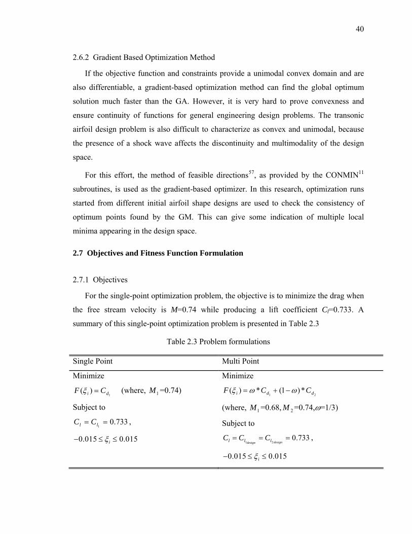
40
2.6.2 Gradient Based Optimization Method
If the objective function and constraints provide a unimodal convex domain and are
also differentiable, a gradient-based optimization method can find the global optimum
solution much faster than the GA. However, it is very hard to prove convexness and
ensure continuity of functions for general engineering design problems. The transonic
airfoil design problem is also difficult to characterize as convex and unimodal, because
the presence of a shock wave affects the discontinuity and multimodality of the design
space.
For this effort, the method of feasible directions57, as provided by the CONMIN11
subroutines, is used as the gradient-based optimizer. In this research, optimization runs
started from different initial airfoil shape designs are used to check the consistency of
optimum points found by the GM. This can give some indication of multiple local
minima appearing in the design space.
2.7 Objectives and Fitness Function Formulation
2.7.1 Objectives
For the single-point optimization problem, the objective is to minimize the drag when
the free stream velocity is M=0.74 while producing a lift coefficient Cl=0.733. A
summary of this single-point optimization problem is presented in Table 2.3
Table 2.3 Problem formulations
Single Point Multi Point
Minimize
1)( di CF =ξ (where, 1M =0.74)
Subject to
733.01
== ll CC ,
0.015 0.015iξ− ≤ ≤
Minimize
21*)1(*)( ddi CCF ωωξ −+=
(where, 1M =0.68, 2M =0.74,ω=1/3)
Subject to
733.021
===designdesign lll CCC ,
0.015 0.015iξ− ≤ ≤
41
A single-point design usually has poor performance in off-design conditions. To
overcome this, a multi-point design is suggested and applied herein. A two-point design
case was set-up to investigate the effects of the objective function selection. The two
design Mach numbers are M=0.68 and M=0.74 as suggested by Drela47. The design lift
coefficient is 0.733 for both Mach numbers. Thus, the drag coefficient at the second
design point (M=0.68) is also included in the objective function Equation (2.4) with the
weighting factor of ω=1/3 in Equation (2.5). To satisfy the lift coefficient condition, the
trimming used in single-point optimization was applied for each design condition
separately, which results in two different angles of attack one for each Mach number. The
computational time of the multi-point design increased to twice that of the single-point
design.
2.7.2 Fitness Function Formulation
For the Genetic Algorithm, constraint violations are added to the objective function
using an exterior penalty. Even though trimming is already applied, a lift coefficient
penalty term is added to the objective function to ensure that the lift coefficient constraint
is satisfied. This is because some airfoil shapes, particularly those in the initial, randomly
generated population, do not have a linear lift curve slope. For convenience, the fitness
function is multiplied by 100 to increase the value, because the order of magnitude of the
drag coefficient is very small. The equality lC constraint has been changed to an
inequality constraint to maintain the error smaller than the tolerance value (ε=0.002, see
Table 2.4).
The input values for GA are described in Table 2.4. The GA begins with a set of
solutions, represented by chromosomes, called the population. Solutions from one
population are taken and selected based on their fitness to form a new population. The
more suitable individuals, represented by binary code, receive more chances to reproduce.
More details of the GA can be found in Ref. 54. The population size and mutation rate
were selected using empirically derived guidelines58 for GA using tournament selection
and uniform crossover. Seven bits represent each of the 16 shape function multipliers, (8
for upper surface and 8 for lower surface) for a total chromosome length of 112 bits.
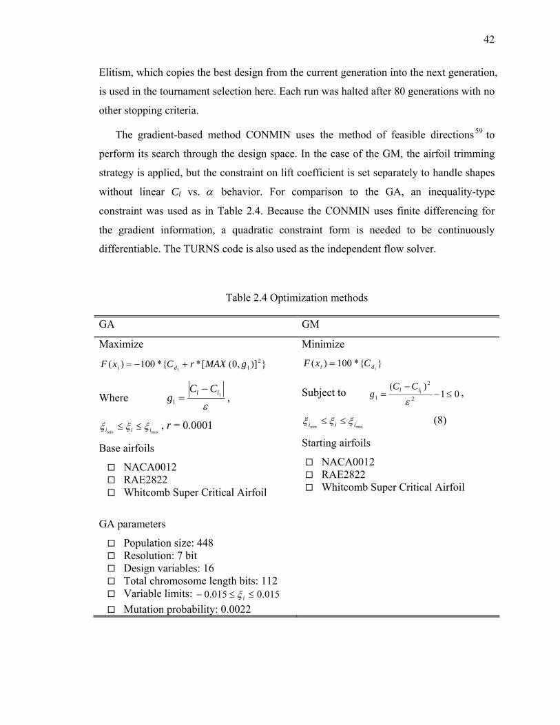
42
Elitism, which copies the best design from the current generation into the next generation,
is used in the tournament selection here. Each run was halted after 80 generations with no
other stopping criteria.
The gradient-based method CONMIN uses the method of feasible directions 59 to
perform its search through the design space. In the case of the GM, the airfoil trimming
strategy is applied, but the constraint on lift coefficient is set separately to handle shapes
without linear Cl vs. α behavior. For comparison to the GA, an inequality-type
constraint was used as in Table 2.4. Because the CONMIN uses finite differencing for
the gradient information, a quadratic constraint form is needed to be continuously
differentiable. The TURNS code is also used as the independent flow solver.
Table 2.4 Optimization methods
GA GM
Maximize
})],0([*{*100)( 211
gMAXrCxF di +−=
Where ε
1
1ll CC
g−
= ,
maxmin iii ξξξ ≤≤ , r = 0.0001
Base airfoils
NACA0012 RAE2822 Whitcomb Super Critical Airfoil
GA parameters
Population size: 448 Resolution: 7 bit Design variables: 16 Total chromosome length bits: 112 Variable limits: 015.0015.0 ≤≤− iξ Mutation probability: 0.0022
Minimize
}{*100)(1di CxF =
Subject to 01)(
2
2
11 ≤−
−=
εll CC
g ,
maxmin iii ξξξ ≤≤ (8)
Starting airfoils
NACA0012 RAE2822 Whitcomb Super Critical Airfoil
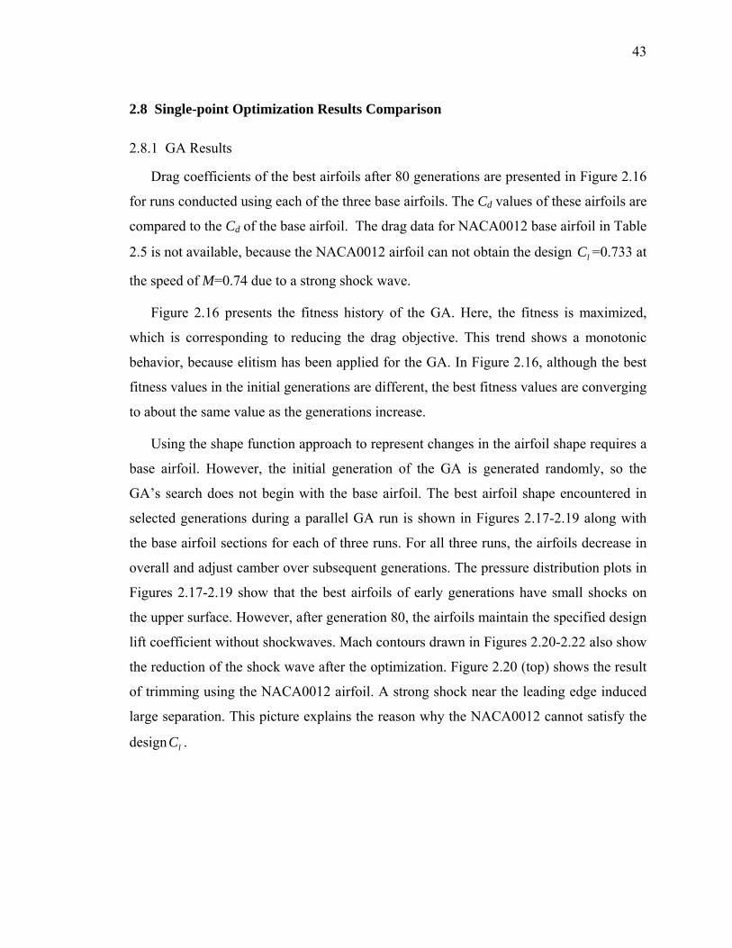
43
2.8 Single-point Optimization Results Comparison
2.8.1 GA Results
Drag coefficients of the best airfoils after 80 generations are presented in Figure 2.16
for runs conducted using each of the three base airfoils. The Cd values of these airfoils are
compared to the Cd of the base airfoil. The drag data for NACA0012 base airfoil in Table
2.5 is not available, because the NACA0012 airfoil can not obtain the design lC =0.733 at
the speed of M=0.74 due to a strong shock wave.
Figure 2.16 presents the fitness history of the GA. Here, the fitness is maximized,
which is corresponding to reducing the drag objective. This trend shows a monotonic
behavior, because elitism has been applied for the GA. In Figure 2.16, although the best
fitness values in the initial generations are different, the best fitness values are converging
to about the same value as the generations increase.
Using the shape function approach to represent changes in the airfoil shape requires a
base airfoil. However, the initial generation of the GA is generated randomly, so the
GA’s search does not begin with the base airfoil. The best airfoil shape encountered in
selected generations during a parallel GA run is shown in Figures 2.17-2.19 along with
the base airfoil sections for each of three runs. For all three runs, the airfoils decrease in
overall and adjust camber over subsequent generations. The pressure distribution plots in
Figures 2.17-2.19 show that the best airfoils of early generations have small shocks on
the upper surface. However, after generation 80, the airfoils maintain the specified design
lift coefficient without shockwaves. Mach contours drawn in Figures 2.20-2.22 also show
the reduction of the shock wave after the optimization. Figure 2.20 (top) shows the result
of trimming using the NACA0012 airfoil. A strong shock near the leading edge induced
large separation. This picture explains the reason why the NACA0012 cannot satisfy the
design lC .
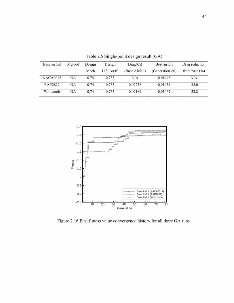
44
Table 2.5 Single-point design result (GA)
Base airfoil Method Design
Mach
Design
Lift Coeff.
Drag(Cd)
(Base Airfoil)
Best airfoil
(Generation-80)
Drag reduction
from base (%)
NACA0012 GA 0.74 0.733 N/A 0.01498 N/A
RAE2822 GA 0.74 0.733 0.02238 0.01454 -35.0
Whitcomb GA 0.74 0.733 0.02189 0.01462 -33.2
10 20 30 40 50 60 70 80Generation
-2.3
-2.2
-2.1
-2
-1.9
-1.8
-1.7
-1.6
-1.5
-1.4
Fitn
ess
Base Airfoil (NACA0012)Base Airfoil (RAE2822)Base Airfoil (Whitcomb)
Figure 2.16 Best fitness value convergence history for all three GA runs.
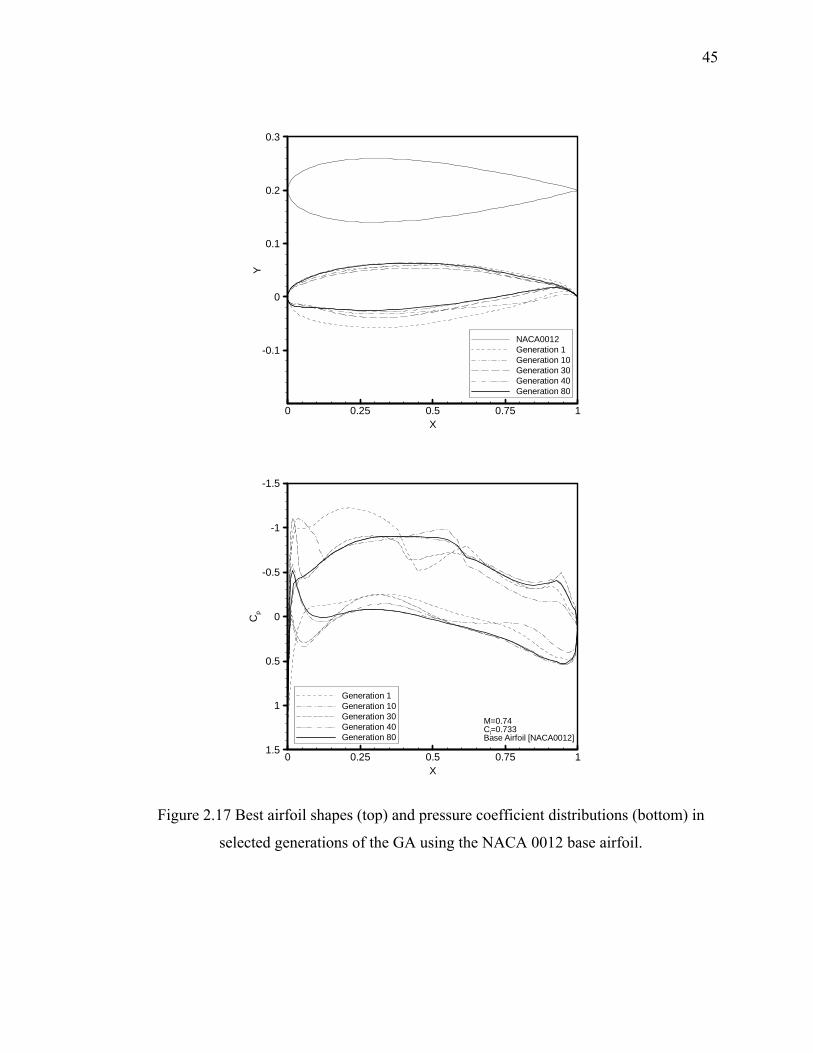
45
0 0.25 0.5 0.75 1X
-0.1
0
0.1
0.2
0.3
Y
NACA0012Generation 1Generation 10Generation 30Generation 40Generation 80
0 0.25 0.5 0.75 1X
-1.5
-1
-0.5
0
0.5
1
1.5
Cp
Generation 1Generation 10Generation 30Generation 40Generation 80
M=0.74Cl=0.733Base Airfoil [NACA0012]
Figure 2.17 Best airfoil shapes (top) and pressure coefficient distributions (bottom) in
selected generations of the GA using the NACA 0012 base airfoil.
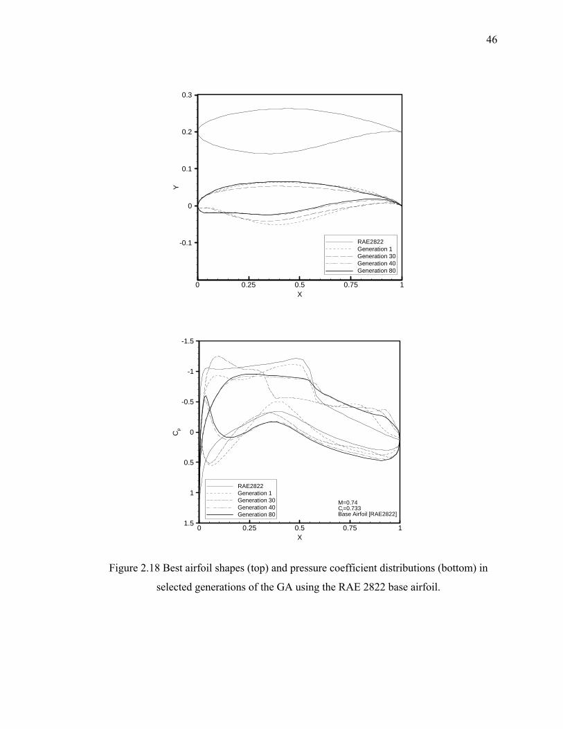
46
0 0.25 0.5 0.75 1X
-0.1
0
0.1
0.2
0.3
Y
RAE2822Generation 1Generation 30Generation 40Generation 80
0 0.25 0.5 0.75 1X
-1.5
-1
-0.5
0
0.5
1
1.5
Cp
RAE2822Generation 1Generation 30Generation 40Generation 80
M=0.74Cl=0.733Base Airfoil [RAE2822]
Figure 2.18 Best airfoil shapes (top) and pressure coefficient distributions (bottom) in
selected generations of the GA using the RAE 2822 base airfoil.
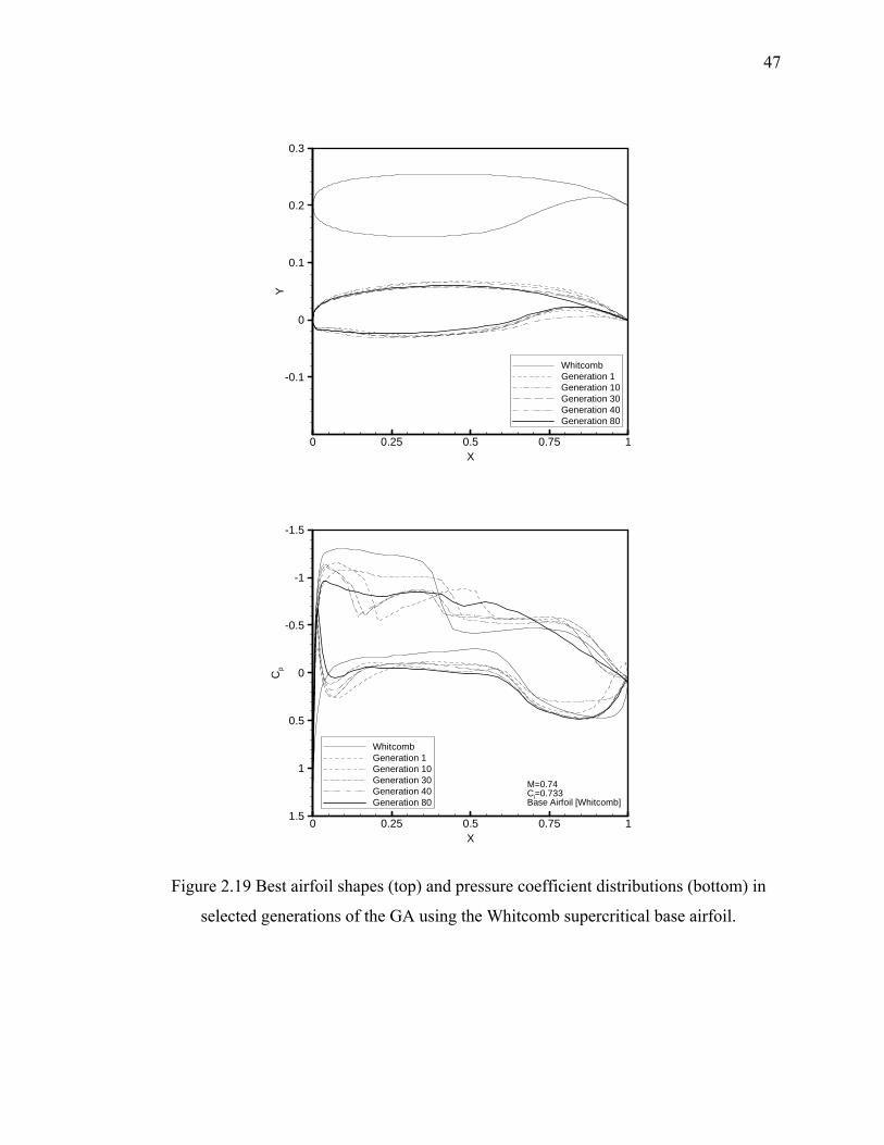
47
0 0.25 0.5 0.75 1X
-0.1
0
0.1
0.2
0.3
Y
WhitcombGeneration 1Generation 10Generation 30Generation 40Generation 80
0 0.25 0.5 0.75 1X
-1.5
-1
-0.5
0
0.5
1
1.5
Cp
WhitcombGeneration 1Generation 10Generation 30Generation 40Generation 80
M=0.74Cl=0.733Base Airfoil [Whitcomb]
Figure 2.19 Best airfoil shapes (top) and pressure coefficient distributions (bottom) in
selected generations of the GA using the Whitcomb supercritical base airfoil.
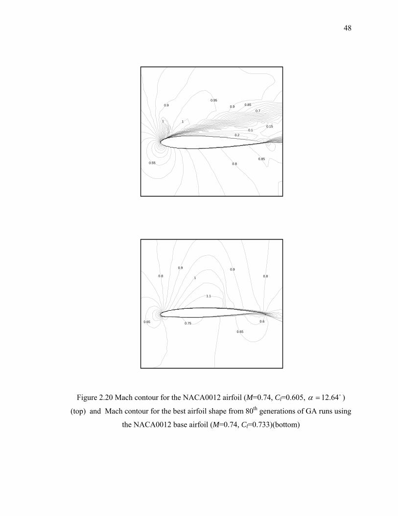
48
11
0.9 0.85
0.1
0.55
0.2
0.15
0.95
0.80.85
0.7
0.9
1
0.9
1.1
0.9
0.80.8
0.65 0.75
0.65
0.6
Figure 2.20 Mach contour for the NACA0012 airfoil (M=0.74, Cl=0.605, 64.12=α )
(top) and Mach contour for the best airfoil shape from 80th generations of GA runs using
the NACA0012 base airfoil (M=0.74, Cl=0.733)(bottom)
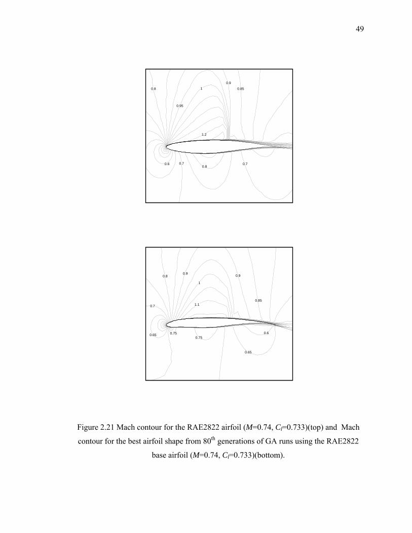
49
1
1.2
0.9
0.85
0.60.8
0.70.7
0.8
0.95
1
1.1
0.90.8
0.7
0.750.75
0.65
0.6
0.85
0.9
0.65
Figure 2.21 Mach contour for the RAE2822 airfoil (M=0.74, Cl=0.733)(top) and Mach
contour for the best airfoil shape from 80th generations of GA runs using the RAE2822
base airfoil (M=0.74, Cl=0.733)(bottom).
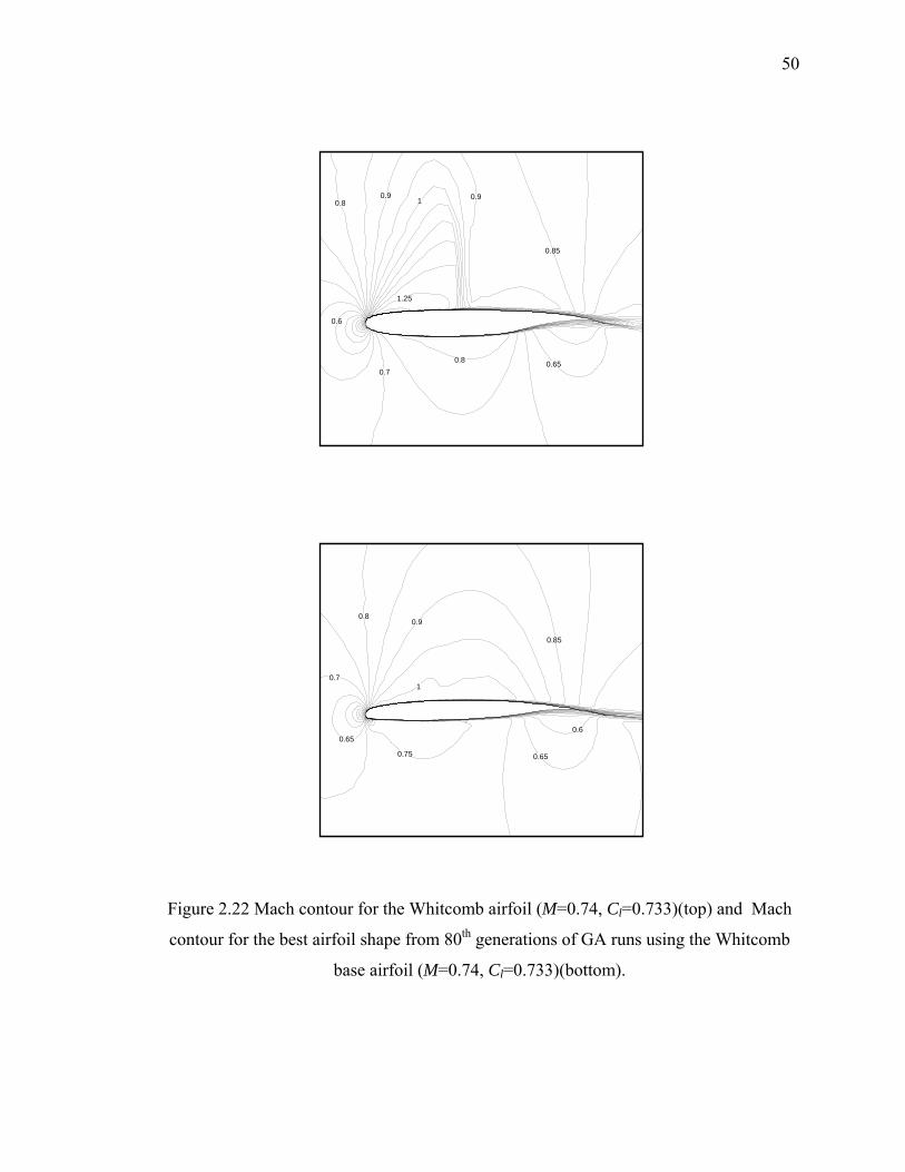
50
1.25
10.9
0.80.9
0.85
0.80.7
0.65
0.6
0.9
1
0.8
0.7
0.75 0.65
0.60.65
0.85
Figure 2.22 Mach contour for the Whitcomb airfoil (M=0.74, Cl=0.733)(top) and Mach
contour for the best airfoil shape from 80th generations of GA runs using the Whitcomb
base airfoil (M=0.74, Cl=0.733)(bottom).
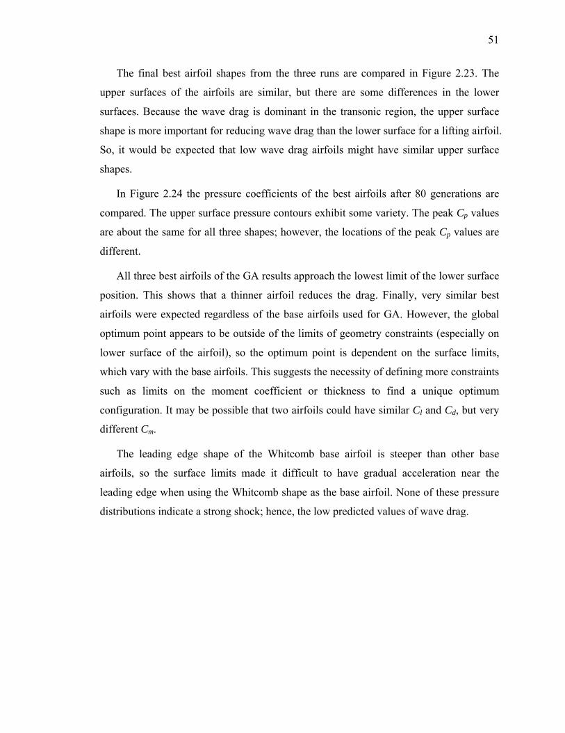
51
The final best airfoil shapes from the three runs are compared in Figure 2.23. The
upper surfaces of the airfoils are similar, but there are some differences in the lower
surfaces. Because the wave drag is dominant in the transonic region, the upper surface
shape is more important for reducing wave drag than the lower surface for a lifting airfoil.
So, it would be expected that low wave drag airfoils might have similar upper surface
shapes.
In Figure 2.24 the pressure coefficients of the best airfoils after 80 generations are
compared. The upper surface pressure contours exhibit some variety. The peak Cp values
are about the same for all three shapes; however, the locations of the peak Cp values are
different.
All three best airfoils of the GA results approach the lowest limit of the lower surface
position. This shows that a thinner airfoil reduces the drag. Finally, very similar best
airfoils were expected regardless of the base airfoils used for GA. However, the global
optimum point appears to be outside of the limits of geometry constraints (especially on
lower surface of the airfoil), so the optimum point is dependent on the surface limits,
which vary with the base airfoils. This suggests the necessity of defining more constraints
such as limits on the moment coefficient or thickness to find a unique optimum
configuration. It may be possible that two airfoils could have similar Cl and Cd, but very
different Cm.
The leading edge shape of the Whitcomb base airfoil is steeper than other base
airfoils, so the surface limits made it difficult to have gradual acceleration near the
leading edge when using the Whitcomb shape as the base airfoil. None of these pressure
distributions indicate a strong shock; hence, the low predicted values of wave drag.
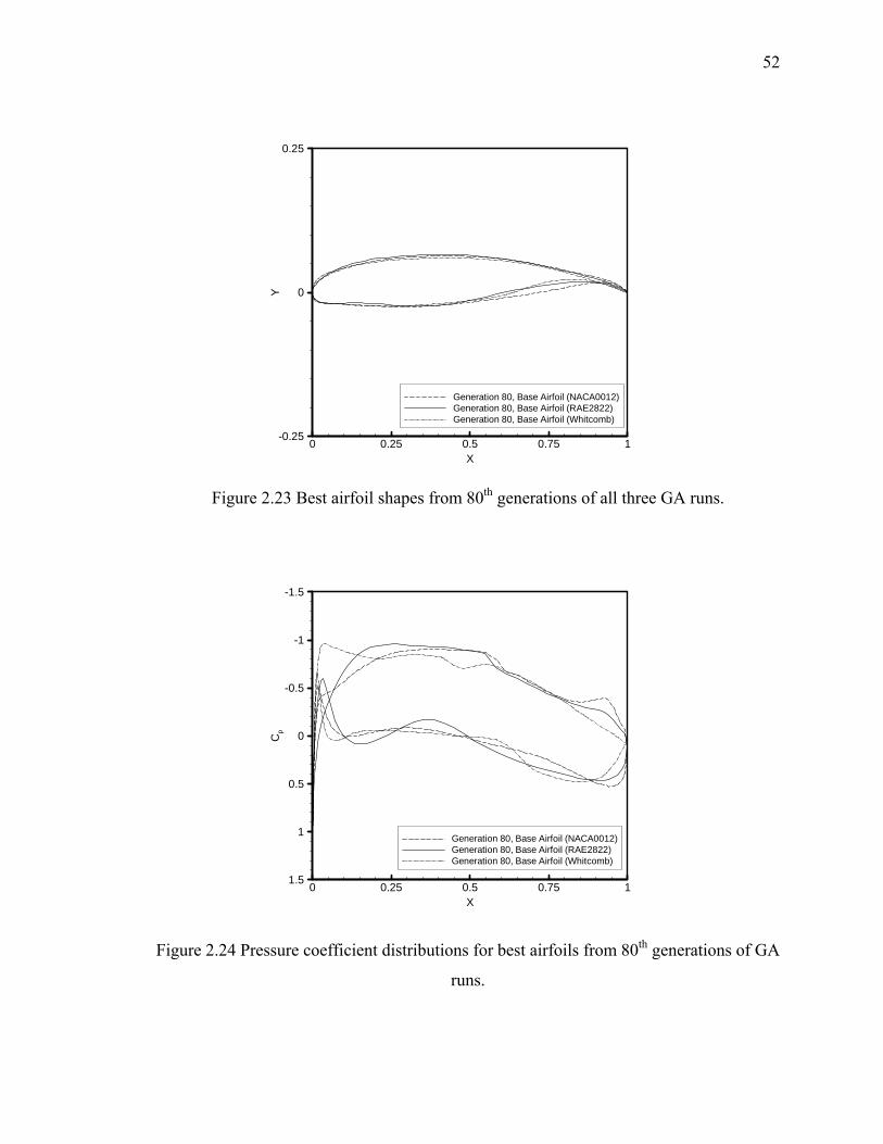
52
0 0.25 0.5 0.75 1X
-0.25
0
0.25
Y
Generation 80, Base Airfoil (NACA0012)Generation 80, Base Airfoil (RAE2822)Generation 80, Base Airfoil (Whitcomb)
Figure 2.23 Best airfoil shapes from 80th generations of all three GA runs.
0 0.25 0.5 0.75 1X
-1.5
-1
-0.5
0
0.5
1
1.5
Cp
Generation 80, Base Airfoil (NACA0012)Generation 80, Base Airfoil (RAE2822)Generation 80, Base Airfoil (Whitcomb)
Figure 2.24 Pressure coefficient distributions for best airfoils from 80th generations of GA
runs.
53
2.8.2 GM Results
The initial design for the search is the base airfoil. Figure 2.25 shows the convergence
history of the CONMIN program using the RAE2822 and the Whitcomb airfoil as the
starting point. In the CONMIN subroutine, the objective and constraint function values
are normalized and adjusted for calculations. In the formulation of the GA fitness
function, it is necessary to find good values for the lift coefficient penalty multiplier.
Similarly, scaling of variables is needed for the GM and to find the proper scale for the
numerical gradient. To determine these, trial and error is required.
When using the NACA0012 as the starting airfoil, CONMIN could not find any
feasible directions because of the strong shock wave associated with the NACA0012 at
the design conditions. As an outcome, no optimized airfoils could be found. This is noted
as N/A in Table 2.6.
Figure 2.26 (top) shows the change of the airfoil shape and the change of pressure
coefficient during the iterations with the RAE2822 as the starting airfoil. Only small
changes to the shape are made during the search. The airfoil is modified to reduce the
shock of the airfoils. The final airfoil surface pressure in Figure 2.26 (bottom) shows a
nearly isentropic compression on the upper surface.
Figure 2.27 also shows that the final airfoil shape does not change much when using
the Whitcomb airfoil as the base shape. The final airfoil starting from the Whitcomb
airfoil also does not have strong shock wave, but the negative peak value of upper surface
pressure is higher than the final airfoil from RAE2822.
A different converged solution was acquired from two different initial airfoils by the
use of the gradient-based search method. This supports the notion that the transonic
airfoil design space has many local optimum design points, and the GM simply finds the
local optimum nearest to the initial airfoil shape.
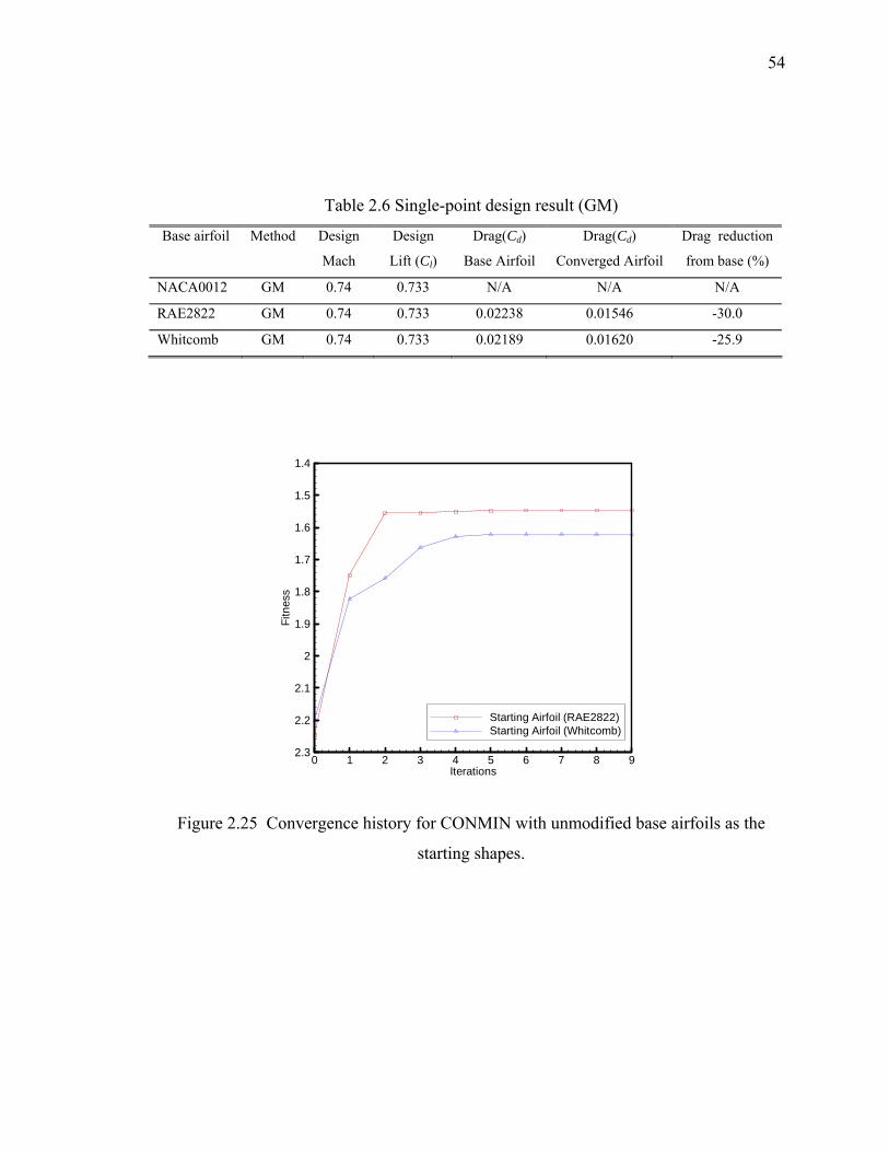
54
Table 2.6 Single-point design result (GM)
Base airfoil Method Design
Mach
Design
Lift (Cl)
Drag(Cd)
Base Airfoil
Drag(Cd)
Converged Airfoil
Drag reduction
from base (%)
NACA0012 GM 0.74 0.733 N/A N/A N/A
RAE2822 GM 0.74 0.733 0.02238 0.01546 -30.0
Whitcomb GM 0.74 0.733 0.02189 0.01620 -25.9
0 1 2 3 4 5 6 7 8 9Iterations
1.4
1.5
1.6
1.7
1.8
1.9
2
2.1
2.2
2.3
Fitn
ess
Starting Airfoil (RAE2822)Starting Airfoil (Whitcomb)
Figure 2.25 Convergence history for CONMIN with unmodified base airfoils as the
starting shapes.
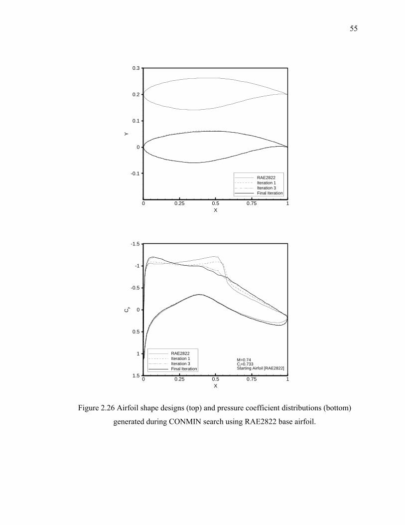
55
0 0.25 0.5 0.75 1X
-0.1
0
0.1
0.2
0.3
Y
RAE2822Iteration 1Iteration 3Final Iteration
0 0.25 0.5 0.75 1X
-1.5
-1
-0.5
0
0.5
1
1.5
Cp
RAE2822Iteration 1Iteration 3Final Iteration
M=0.74Cl=0.733Starting Airfoil [RAE2822]
Figure 2.26 Airfoil shape designs (top) and pressure coefficient distributions (bottom)
generated during CONMIN search using RAE2822 base airfoil.
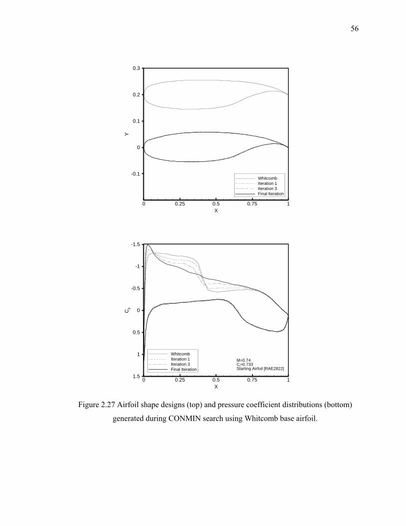
56
0 0.25 0.5 0.75 1X
-0.1
0
0.1
0.2
0.3
Y
WhitcombIteration 1Iteration 3Final Iteration
0 0.25 0.5 0.75 1X
-1.5
-1
-0.5
0
0.5
1
1.5
Cp
WhitcombIteration 1Iteration 3Final Iteration
M=0.74Cl=0.733Starting Airfoil [RAE2822]
Figure 2.27 Airfoil shape designs (top) and pressure coefficient distributions (bottom)
generated during CONMIN search using Whitcomb base airfoil.
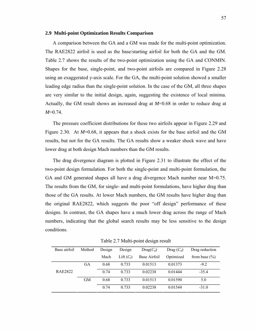
57
2.9 Multi-point Optimization Results Comparison
A comparison between the GA and a GM was made for the multi-point optimization.
The RAE2822 airfoil is used as the base/starting airfoil for both the GA and the GM.
Table 2.7 shows the results of the two-point optimization using the GA and CONMIN.
Shapes for the base, single-point, and two-point airfoils are compared in Figure 2.28
using an exaggerated y-axis scale. For the GA, the multi-point solution showed a smaller
leading edge radius than the single-point solution. In the case of the GM, all three shapes
are very similar to the initial design, again, suggesting the existence of local minima.
Actually, the GM result shows an increased drag at M=0.68 in order to reduce drag at
M=0.74.
The pressure coefficient distributions for these two airfoils appear in Figure 2.29 and
Figure 2.30. At M=0.68, it appears that a shock exists for the base airfoil and the GM
results, but not for the GA results. The GA results show a weaker shock wave and have
lower drag at both design Mach numbers than the GM results.
The drag divergence diagram is plotted in Figure 2.31 to illustrate the effect of the
two-point design formulation. For both the single-point and multi-point formulation, the
GA and GM generated shapes all have a drag divergence Mach number near M=0.75.
The results from the GM, for single- and multi-point formulations, have higher drag than
those of the GA results. At lower Mach numbers, the GM results have higher drag than
the original RAE2822, which suggests the poor “off design” performance of these
designs. In contrast, the GA shapes have a much lower drag across the range of Mach
numbers, indicating that the global search results may be less sensitive to the design
conditions.
Table 2.7 Multi-point design result
Base airfoil Method Design
Mach
Design
Lift (Cl)
Drag(Cd)
Base Airfoil
Drag (Cd)
Optimized
Drag reduction
from base (%)
0.68 0.733 0.01513 0.01373 -9.2 GA
0.74 0.733 0.02238 0.01444 -35.4
0.68 0.733 0.01513 0.01590 5.0
RAE2822
GM
0.74 0.733 0.02238 0.01544 -31.0
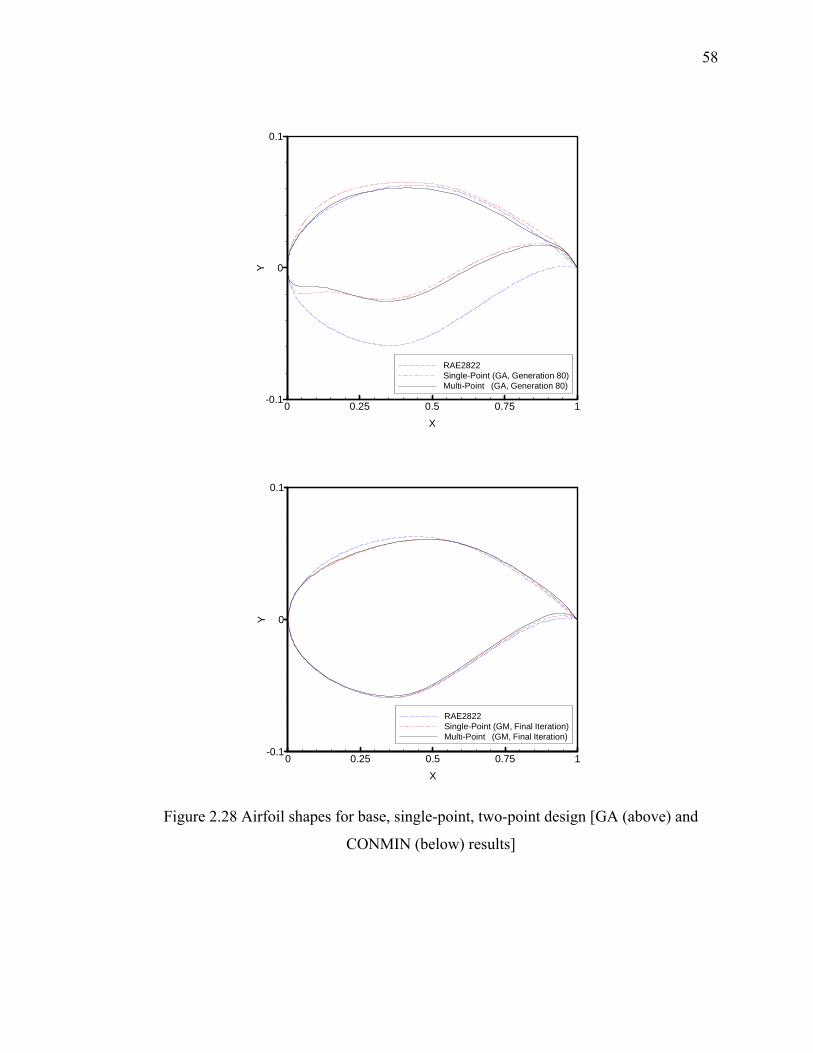
58
0 0.25 0.5 0.75 1
X
-0.1
0
0.1
Y
RAE2822Single-Point (GA, Generation 80)Multi-Point (GA, Generation 80)
0 0.25 0.5 0.75 1
X
-0.1
0
0.1
Y
RAE2822Single-Point (GM, Final Iteration)Multi-Point (GM, Final Iteration)
Figure 2.28 Airfoil shapes for base, single-point, two-point design [GA (above) and
CONMIN (below) results]
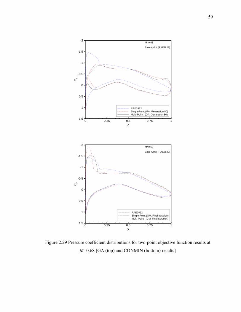
59
0 0.25 0.5 0.75 1X
-2
-1.5
-1
-0.5
0
0.5
1
1.5
Cp
RAE2822Single-Point (GA, Generation 80)Multi-Point (GA, Generation 80)
M=0.68
Base Airfoil [RAE2822]
0 0.25 0.5 0.75 1X
-2
-1.5
-1
-0.5
0
0.5
1
1.5
Cp
RAE2822Single-Point (GM, Final Iteration)Multi-Point (GM, Final Iteration)
M=0.68
Base Airfoil [RAE2822]
Figure 2.29 Pressure coefficient distributions for two-point objective function results at
M=0.68 [GA (top) and CONMIN (bottom) results]
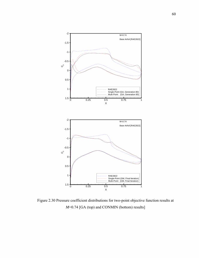
60
0 0.25 0.5 0.75 1X
-2
-1.5
-1
-0.5
0
0.5
1
1.5
Cp
RAE2822Single-Point (GA, Generation 80)Multi-Point (GA, Generation 80)
M=0.74
Base Airfoil [RAE2822]
0 0.25 0.5 0.75 1X
-2
-1.5
-1
-0.5
0
0.5
1
1.5
Cp
RAE2822Single-Point (GM, Final Iteration)Multi-Point (GM, Final Iteration)
M=0.74
Base Airfoil [RAE2822]
Figure 2.30 Pressure coefficient distributions for two-point objective function results at
M=0.74 [GA (top) and CONMIN (bottom) results]
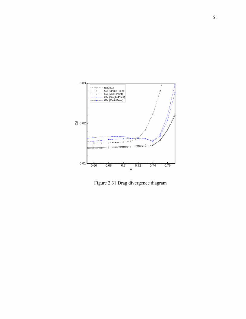
61
0.66 0.68 0.7 0.72 0.74 0.76M
0.01
0.02
0.03
Cd
rae2822GA (Single-Point)GA (Multi-Point)GM (Single-Point)GM (Multi-Point)
Figure 2.31 Drag divergence diagram
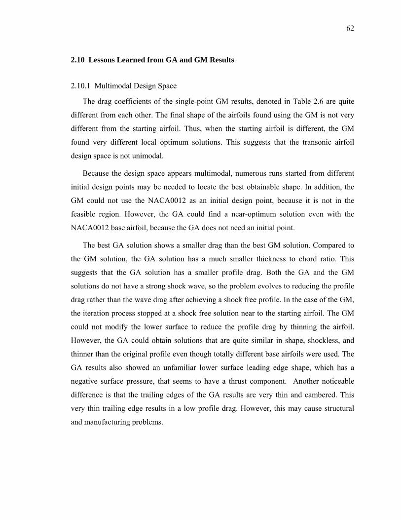
62
2.10 Lessons Learned from GA and GM Results
2.10.1 Multimodal Design Space
The drag coefficients of the single-point GM results, denoted in Table 2.6 are quite
different from each other. The final shape of the airfoils found using the GM is not very
different from the starting airfoil. Thus, when the starting airfoil is different, the GM
found very different local optimum solutions. This suggests that the transonic airfoil
design space is not unimodal.
Because the design space appears multimodal, numerous runs started from different
initial design points may be needed to locate the best obtainable shape. In addition, the
GM could not use the NACA0012 as an initial design point, because it is not in the
feasible region. However, the GA could find a near-optimum solution even with the
NACA0012 base airfoil, because the GA does not need an initial point.
The best GA solution shows a smaller drag than the best GM solution. Compared to
the GM solution, the GA solution has a much smaller thickness to chord ratio. This
suggests that the GA solution has a smaller profile drag. Both the GA and the GM
solutions do not have a strong shock wave, so the problem evolves to reducing the profile
drag rather than the wave drag after achieving a shock free profile. In the case of the GM,
the iteration process stopped at a shock free solution near to the starting airfoil. The GM
could not modify the lower surface to reduce the profile drag by thinning the airfoil.
However, the GA could obtain solutions that are quite similar in shape, shockless, and
thinner than the original profile even though totally different base airfoils were used. The
GA results also showed an unfamiliar lower surface leading edge shape, which has a
negative surface pressure, that seems to have a thrust component. Another noticeable
difference is that the trailing edges of the GA results are very thin and cambered. This
very thin trailing edge results in a low profile drag. However, this may cause structural
and manufacturing problems.
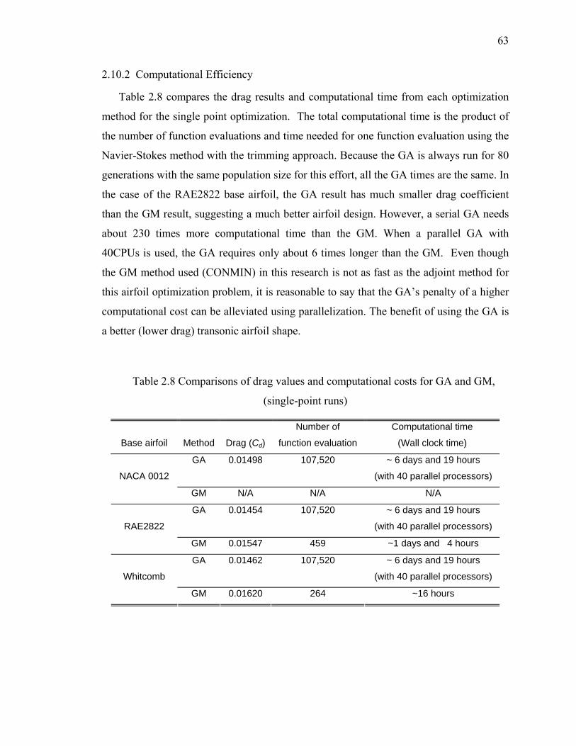
63
2.10.2 Computational Efficiency
Table 2.8 compares the drag results and computational time from each optimization
method for the single point optimization. The total computational time is the product of
the number of function evaluations and time needed for one function evaluation using the
Navier-Stokes method with the trimming approach. Because the GA is always run for 80
generations with the same population size for this effort, all the GA times are the same. In
the case of the RAE2822 base airfoil, the GA result has much smaller drag coefficient
than the GM result, suggesting a much better airfoil design. However, a serial GA needs
about 230 times more computational time than the GM. When a parallel GA with
40CPUs is used, the GA requires only about 6 times longer than the GM. Even though
the GM method used (CONMIN) in this research is not as fast as the adjoint method for
this airfoil optimization problem, it is reasonable to say that the GA’s penalty of a higher
computational cost can be alleviated using parallelization. The benefit of using the GA is
a better (lower drag) transonic airfoil shape.
Table 2.8 Comparisons of drag values and computational costs for GA and GM,
(single-point runs)
Base airfoil
Method
Drag (Cd)
Number of
function evaluation
Computational time
(Wall clock time)
GA 0.01498 107,520 ~ 6 days and 19 hours
(with 40 parallel processors)
NACA 0012
GM N/A N/A N/A
GA 0.01454 107,520 ~ 6 days and 19 hours
(with 40 parallel processors)
RAE2822
GM 0.01547 459 ~1 days and 4 hours
GA 0.01462 107,520 ~ 6 days and 19 hours
(with 40 parallel processors)
Whitcomb
GM 0.01620 264 ~16 hours
64
2.11 Summary
A manager-worker type parallel Genetic Algorithm has been developed and applied
for the transonic airfoil design problem.
The parameterization of the airfoil shape is one important issue that was investigated.
A simple reconstruction test showed that the analytical method using shape functions can
have good accuracy while keeping reasonable shapes. However, the selection of the base
airfoil is important for this method for both the GM and the GA.
Trimming is an another issue for optimization especially for the GA. Trimming can
simplify the design space, however, adding an external penalty type constraint is still
necessary to limit the computational cost increase.
Both the GA and the GM found shock-free airfoils. However, the GA results showed
smaller total drag than the GM results. This suggests the GA results have a smaller
profile drag than the GM results and the GA was not affected by the shock-free local
minima in transonic flow. Thus, by using the GA new shapes for the lower surfaces were
found.
The GM stopped at different shock-free conditions when changing the starting airfoil.
This suggests that the design space of transonic airfoil has probably numerous local
optimum points. The GA found airfoils with similar upper surface shapes. However, the
lower surfaces were different, because they are limited by the boundaries of the design
space. This implies that the global optimum point is outside of the boundaries for the
lower surfaces. This result suggests that it is an issue for using the GA to define a design
space boundary that includes the global optimum design.
Parallelization is a key issue in using the GA method in transonic airfoil optimization.
Without using parallel computing, the GA requires unrealistic CPU time when combined
with a high fidelity numerical solver such as a Navier-stokes solver. The nature of the
population-based search with small communication requirements makes the GA suitable
for an efficient parallelization and reduces the significant computation time to an
affordable level.
65
CHAPTER 3 AIRFOIL OPTIMIZATION FOR MORPHING AIRCRAFT
By varying the wing’s airfoil shape in flight, a morphing aircraft could meet a single
point aerodynamic objective at each point in its flight envelope. However, morphing
aircraft will require an actuation system to morph their shapes. One of the objectives of
this research is to include a measure of the energy needed for morphing as part of the
design objectives. This research is under the assumption that the energy needed to change
airfoil shape will be proportional to the actuation system weight.
A simple strain energy model has been introduced in Ref. 39 as an objective to
consider the shape variation of an aircraft wing. Prock39, et al. suggested a single-
objective optimization approach, that is setting the strain energy as a single objective
while addressing the aerodynamic performance via constraints.
In this research, a multi-objective optimization strategy is proposed instead of a single
objective approach. The relative strain energy is used as another design objective along
with a combined drag coefficient objective. Three different multi-objective optimization
methods are applied to this problem. Guided by the conclusions of Chapter 2, the parallel
GA is selected as an optimization algorithm for the airfoil optimization of a morphing
aircraft.
3.1 Problem Description
Some recent studies 60 by the US Air Force Research Laboratory (AFRL) have
focused upon a high-altitude, long-endurance aircraft platform. A notional representation
of this concept appears in Figure 3.1. This aircraft’s design mission includes a 40+ hour
loiter segment, during which the aircraft will experience a significant weight reduction as
it consumes most of its fuel. If the aircraft is intended to loiter at a constant altitude and
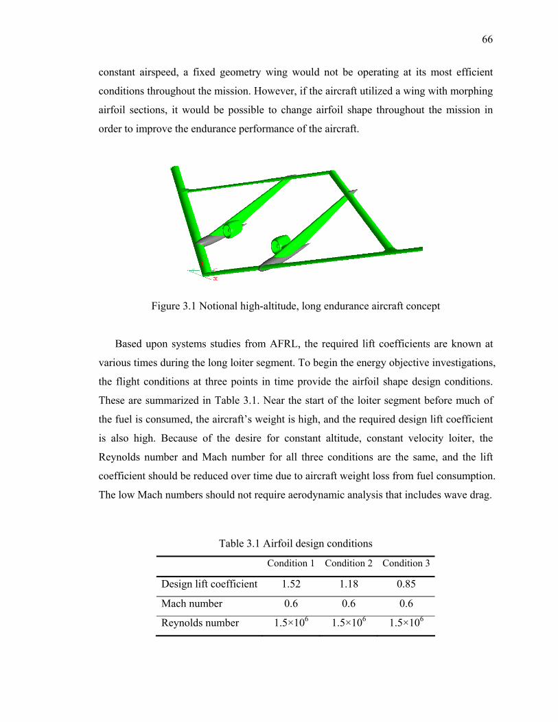
66
constant airspeed, a fixed geometry wing would not be operating at its most efficient
conditions throughout the mission. However, if the aircraft utilized a wing with morphing
airfoil sections, it would be possible to change airfoil shape throughout the mission in
order to improve the endurance performance of the aircraft.
Figure 3.1 Notional high-altitude, long endurance aircraft concept
Based upon systems studies from AFRL, the required lift coefficients are known at
various times during the long loiter segment. To begin the energy objective investigations,
the flight conditions at three points in time provide the airfoil shape design conditions.
These are summarized in Table 3.1. Near the start of the loiter segment before much of
the fuel is consumed, the aircraft’s weight is high, and the required design lift coefficient
is also high. Because of the desire for constant altitude, constant velocity loiter, the
Reynolds number and Mach number for all three conditions are the same, and the lift
coefficient should be reduced over time due to aircraft weight loss from fuel consumption.
The low Mach numbers should not require aerodynamic analysis that includes wave drag.
Table 3.1 Airfoil design conditions
Condition 1 Condition 2 Condition 3
Design lift coefficient 1.52 1.18 0.85
Mach number 0.6 0.6 0.6
Reynolds number 1.5×10⁶ 1.5×10⁶ 1.5×10⁶
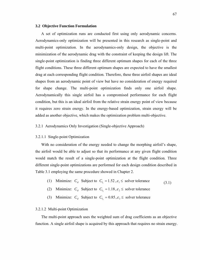
67
3.2 Objective Function Formulation
A set of optimization runs are conducted first using only aerodynamic concerns.
Aerodynamics-only optimization will be presented in this research as single-point and
multi-point optimization. In the aerodynamics-only design, the objective is the
minimization of the aerodynamic drag with the constraint of keeping the design lift. The
single-point optimization is finding three different optimum shapes for each of the three
flight conditions. These three different optimum shapes are expected to have the smallest
drag at each corresponding flight condition. Therefore, these three airfoil shapes are ideal
shapes from an aerodynamic point of view but have no consideration of energy required
for shape change. The multi-point optimization finds only one airfoil shape.
Aerodynamically this single airfoil has a compromised performance for each flight
condition, but this is an ideal airfoil from the relative strain energy point of view because
it requires zero strain energy. In the energy-based optimization, strain energy will be
added as another objective, which makes the optimization problem multi-objective.
3.2.1 Aerodynamics Only Investigation (Single-objective Approach)
3.2.1.1 Single-point Optimization
With no consideration of the energy needed to change the morphing airfoil’s shape,
the airfoil would be able to adjust so that its performance at any given flight condition
would match the result of a single-point optimization at the flight condition. Three
different single-point optimizations are performed for each design condition described in
Table 3.1 employing the same procedure showed in Chapter 2.
(1) Minimize: dC Subject to 52.11
=lC , ≤1ε solver tolerance
(2) Minimize: dC Subject to 18.12
=lC , ≤2ε solver tolerance
(3) Minimize: dC Subject to 85.03
=lC , ≤3ε solver tolerance
(3.1)
3.2.1.2 Multi-point Optimization
The multi-point approach uses the weighted sum of drag coefficients as an objective
function. A single airfoil shape is acquired by this approach that requires no strain energy.
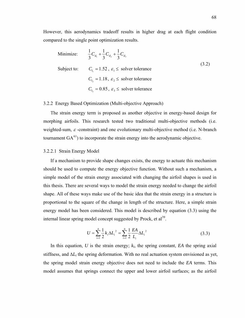
68
However, this aerodynamics tradeoff results in higher drag at each flight condition
compared to the single point optimization results.
Minimize: 321 3
131
31
ddd CCC ++
Subject to: 52.11
=lC , ≤1ε solver tolerance
18.12
=lC , ≤2ε solver tolerance
85.03
=lC , ≤3ε solver tolerance
(3.2)
3.2.2 Energy Based Optimization (Multi-objective Approach)
The strain energy term is proposed as another objective in energy-based design for
morphing airfoils. This research tested two traditional multi-objective methods (i.e.
weighted-sum, ε -constraint) and one evolutionary multi-objective method (i.e. N-branch
tournament GA61) to incorporate the strain energy into the aerodynamic objective.
3.2.2.1 Strain Energy Model
If a mechanism to provide shape changes exists, the energy to actuate this mechanism
should be used to compute the energy objective function. Without such a mechanism, a
simple model of the strain energy associated with changing the airfoil shapes is used in
this thesis. There are several ways to model the strain energy needed to change the airfoil
shape. All of these ways make use of the basic idea that the strain energy in a structure is
proportional to the square of the change in length of the structure. Here, a simple strain
energy model has been considered. This model is described by equation (3.3) using the
internal linear spring model concept suggested by Prock, et al39.
∑∑==
Δ=Δ=n
ii
i
n
iii L
LEALkU
1
2
1
2
21
21 (3.3)
In this equation, U is the strain energy; ki, the spring constant, EA the spring axial
stiffness, and ΔLi the spring deformation. With no real actuation system envisioned as yet,
the spring model strain energy objective does not need to include the EA terms. This
model assumes that springs connect the upper and lower airfoil surfaces; as the airfoil
69
morphs, the springs deform, which corresponds to an amount of strain energy. Figure 3.2
presents a simple illustration of this model. These springs are connected at points
corresponding to the ends of panels used by the aerodynamic analysis.
Internal springs connecting upper and lower surface
icL )/(Δ
icL )/(
Springs contract (or expand) to meet new airfoil shape
Figure 3.2 Internal linear spring model for strain energy
3.2.3 Multi-objective Optimization
When an optimization problem involves more than one objective function, the task of
finding the optimum is known as multi-objective optimization. For a multi-objective
optimization, the objective function is the vector-valued function as shown in Equation
(3.4).
Tk xfxfxfxf )](),...,(),([)( 21= (3.4)
In problems with more than one objectives, there is no single optimum solution.
There exist a number of solutions that are all considered optimal because tradeoffs
between conflicting objectives are important. Without any further information, no
solution from the set of optimal solutions can be said to be better than any other.
The decision variables Fx ∈* is Pareto optimal if there does not exist another
Fx ∈ such that )()( *xfxf ii ≤ for all ki ,...,1= and )()( *xfxf jj < for at least one j. This
definition says that *x is Pareto optimal if there exists no feasible vector of decision
variables Fx ∈ that would decrease some criterion without causing a simultaneous
increase in at least one other criterion. This concept almost always gives not a single
70
solution, but rather a set of solutions called the Pareto optimal set. The vectors *x corresponding to the solutions included in the Pareto optimal set are called
nondominated. The plot of the objective functions whose nondominated vectors are in the
Pareto optimal set is called the Pareto front (or Pareto frontier).
Several approaches have been proposed to find the Pareto optimal set. In this research,
a weighted sum method and constraint-ε methods are used as a first step to explore the
Pareto optimal set.
The weighted sum method combines a set of objectives into a single objective by pre-
multiplying each objective with a user-supplied weight and adding the weighted
objectives. The weight of an objective is usually chosen in proportion to the objective’s
relative importance in the problem. This method is the simplest approach and is easy to
implement. However, linear combinations of weights do not work when the Pareto front
is concave, regardless of the weight used.
To alleviate the difficulties faced by the weighed sum approach in solving problems
having nonconvex objective spaces, the constraint-ε method is used. This method keeps
one of the objectives and restricts the rest of the objectives within user-specified values.
The advantage of this method is that it can be used for any arbitrary problem with either
convex or nonconvex objective space. However, a vector of ε values determining the
location of the Pareto-optimal solution is needed.
3.2.3.1 Weighted Sum Approach
In the weighted sum approach, the strain energy term is added to the aerodynamic
term with a weight factor as denoted in Equation (3.5). The number of all the relative
strain energies (i.e. the change in strain energy when moving from any design shape to
another shape) between the N different airfoils is⎟⎟⎠
⎞⎜⎜⎝
⎛2N . In the case of three different
design conditions, there exist three different relative energies ( 12U , 23U , 13U ). The
definition of the strain energy is the same as shown in Equation (3.3). Instead of using the
sum of the three relative energies, the maximum value of the relative energies is used as
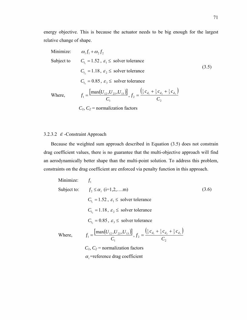
71
energy objective. This is because the actuator needs to be big enough for the largest
relative change of shape.
Minimize: 2211 ff ωω +
Subject to 52.11
=lC , ≤1ε solver tolerance
18.12
=lC , ≤2ε solver tolerance
85.03
=lC , ≤3ε solver tolerance
Where, ( )[ ]
1
1323121
,,maxC
UUUf = ,( )
2
31
31
31
2321
Cccc
f ddd ++=
C1, C2 = normalization factors
(3.5)
3.2.3.2 ε -Constraint Approach
Because the weighted sum approach described in Equation (3.5) does not constrain
drag coefficient values, there is no guarantee that the multi-objective approach will find
an aerodynamically better shape than the multi-point solution. To address this problem,
constraints on the drag coefficient are enforced via penalty function in this approach.
Minimize: 1f
Subject to: if α≤2 (i=1,2,….m)
52.11
=lC , ≤1ε solver tolerance
18.12
=lC , ≤2ε solver tolerance
85.03
=lC , ≤3ε solver tolerance
Where, ( )[ ]1
1323121
,,maxC
UUUf = ,( )
2
31
31
31
2321
Cccc
f ddd ++=
C1, C2 = normalization factors
iα =reference drag coefficient
(3.6)
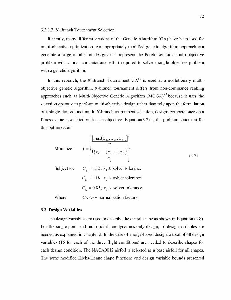
72
3.2.3.3 N-Branch Tournament Selection
Recently, many different versions of the Genetic Algorithm (GA) have been used for
multi-objective optimization. An appropriately modified genetic algorithm approach can
generate a large number of designs that represent the Pareto set for a multi-objective
problem with similar computational effort required to solve a single objective problem
with a genetic algorithm.
In this research, the N-Branch Tournament GA61 is used as a evolutionary multi-
objective genetic algorithm. N-branch tournament differs from non-dominance ranking
approaches such as Multi-Objective Genetic Algorithm (MOGA)62 because it uses the
selection operator to perform multi-objective design rather than rely upon the formulation
of a single fitness function. In N-branch tournament selection, designs compete once on a
fitness value associated with each objective. Equation(3.7) is the problem statement for
this optimization.
Minimize:
( )[ ]
( )⎪⎪⎭
⎪⎪⎬
⎫
⎪⎪⎩
⎪⎪⎨
⎧
++=
2
31
31
31
1
132312
321
,,max
Cccc
CUUU
fddd
Subject to: 52.11
=lC , ≤1ε solver tolerance
18.12
=lC , ≤2ε solver tolerance
85.03
=lC , ≤3ε solver tolerance
Where, C1, C2 = normalization factors
(3.7)
3.3 Design Variables
The design variables are used to describe the airfoil shape as shown in Equation (3.8).
For the single-point and multi-point aerodynamics-only design, 16 design variables are
needed as explained in Chapter 2. In the case of energy-based design, a total of 48 design
variables (16 for each of the three flight conditions) are needed to describe shapes for
each design condition. The NACA0012 airfoil is selected as a base airfoil for all shapes.
The same modified Hicks-Henne shape functions and design variable bounds presented
73
in Chapter 2 are used here. Thus, the same limits on upper and lower surface shapes are
provided.
∑+= )()()( Airfoil) (Base xfxyxy kikikk ξ
( kiξ : Design Variables, kif : Shape Functions)
(3.8)
3.3.1 Optimization Algorithm
The parallel genetic algorithm is used as an optimization algorithm as described
previously in Chapter 2. However, for the multiobjective design with energy as an
objective, the population size and other GA parameters are adjusted as follows (based on
the criteria of Reference 58), because the number of variables is increased to 48.
• Number of design variables = 48
• Bits per design variable = 7 bit
• Chromosome length = 336
• Population size = 1344
• Mutation probability = 0.00037
• Design variable limits = 015.0015.0 ≤≤− iξ
3.3.2 Flow Solver
In this stage of the research, a quick turn-around computational time is desired for the
flow evaluation. Thus, the well-known XFOIL63 code is selected as a function evaluator.
XFOIL uses a linear-vorticity panel method with a Karman-Tsien compressibility
correction for inviscid calculations. To model viscous layer influence, source
distributions are superimposed on the airfoil and wake. The boundary layer and the
transition equations are solved simultaneously with the inviscid flow field by a global
Newton method. At high angles of attack, XFOIL has difficulties obtaining a converged
solution as stall is approached. To prevent this problem, non converged solutions are
given a high penalty by setting the fitness function arbitrarily large via a penalty function
and are eventually eliminated during the design process. The solver tolerance value that
used for this penalty calculation is 0.002.
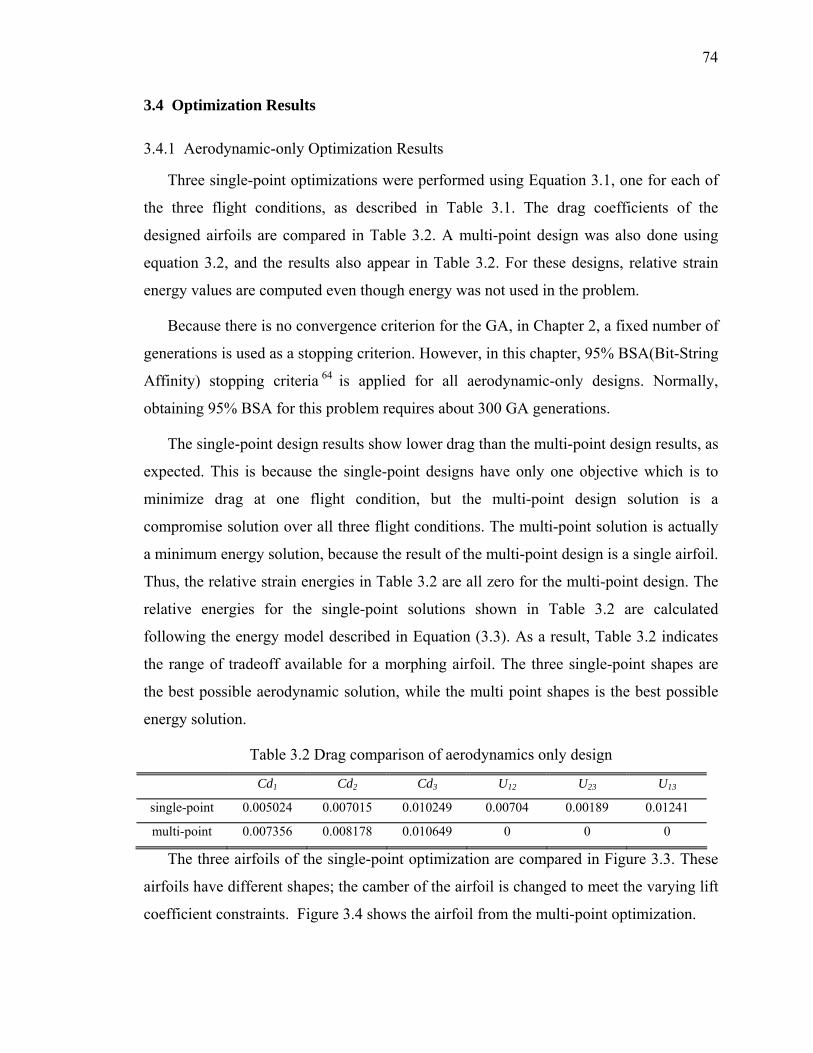
74
3.4 Optimization Results
3.4.1 Aerodynamic-only Optimization Results
Three single-point optimizations were performed using Equation 3.1, one for each of
the three flight conditions, as described in Table 3.1. The drag coefficients of the
designed airfoils are compared in Table 3.2. A multi-point design was also done using
equation 3.2, and the results also appear in Table 3.2. For these designs, relative strain
energy values are computed even though energy was not used in the problem.
Because there is no convergence criterion for the GA, in Chapter 2, a fixed number of
generations is used as a stopping criterion. However, in this chapter, 95% BSA(Bit-String
Affinity) stopping criteria 64 is applied for all aerodynamic-only designs. Normally,
obtaining 95% BSA for this problem requires about 300 GA generations.
The single-point design results show lower drag than the multi-point design results, as
expected. This is because the single-point designs have only one objective which is to
minimize drag at one flight condition, but the multi-point design solution is a
compromise solution over all three flight conditions. The multi-point solution is actually
a minimum energy solution, because the result of the multi-point design is a single airfoil.
Thus, the relative strain energies in Table 3.2 are all zero for the multi-point design. The
relative energies for the single-point solutions shown in Table 3.2 are calculated
following the energy model described in Equation (3.3). As a result, Table 3.2 indicates
the range of tradeoff available for a morphing airfoil. The three single-point shapes are
the best possible aerodynamic solution, while the multi point shapes is the best possible
energy solution.
Table 3.2 Drag comparison of aerodynamics only design
Cd1 Cd2 Cd3 U12 U23 U13
single-point 0.005024 0.007015 0.010249 0.00704 0.00189 0.01241
multi-point 0.007356 0.008178 0.010649 0 0 0
The three airfoils of the single-point optimization are compared in Figure 3.3. These
airfoils have different shapes; the camber of the airfoil is changed to meet the varying lift
coefficient constraints. Figure 3.4 shows the airfoil from the multi-point optimization.
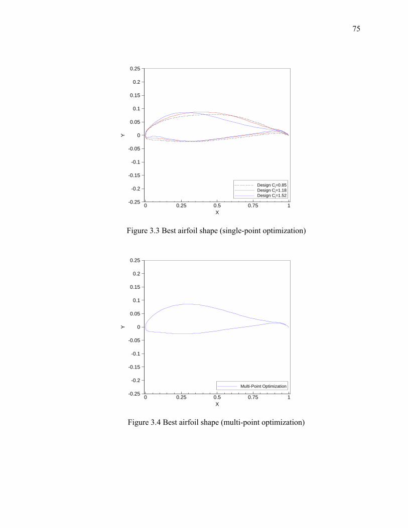
75
0 0.25 0.5 0.75 1X
-0.25
-0.2
-0.15
-0.1
-0.05
0
0.05
0.1
0.15
0.2
0.25
Y
Design Cl=0.85Design Cl=1.18Design Cl=1.52
Figure 3.3 Best airfoil shape (single-point optimization)
0 0.25 0.5 0.75 1X
-0.25
-0.2
-0.15
-0.1
-0.05
0
0.05
0.1
0.15
0.2
0.25
Y
Multi-Point Optimization
Figure 3.4 Best airfoil shape (multi-point optimization)
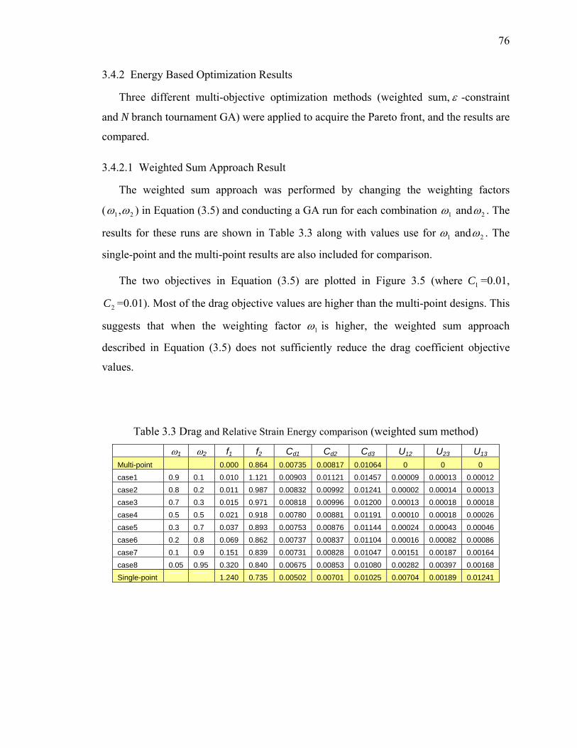
76
3.4.2 Energy Based Optimization Results
Three different multi-objective optimization methods (weighted sum, ε -constraint
and N branch tournament GA) were applied to acquire the Pareto front, and the results are
compared.
3.4.2.1 Weighted Sum Approach Result
The weighted sum approach was performed by changing the weighting factors
( 21,ωω ) in Equation (3.5) and conducting a GA run for each combination 1ω and 2ω . The
results for these runs are shown in Table 3.3 along with values use for 1ω and 2ω . The
single-point and the multi-point results are also included for comparison.
The two objectives in Equation (3.5) are plotted in Figure 3.5 (where 1C =0.01,
2C =0.01). Most of the drag objective values are higher than the multi-point designs. This
suggests that when the weighting factor 1ω is higher, the weighted sum approach
described in Equation (3.5) does not sufficiently reduce the drag coefficient objective
values.
Table 3.3 Drag and Relative Strain Energy comparison (weighted sum method)
ω1 ω2 f1 f2 Cd1 Cd2 Cd3 U12 U23 U13 Multi-point 0.000 0.864 0.00735 0.00817 0.01064 0 0 0 case1 0.9 0.1 0.010 1.121 0.00903 0.01121 0.01457 0.00009 0.00013 0.00012 case2 0.8 0.2 0.011 0.987 0.00832 0.00992 0.01241 0.00002 0.00014 0.00013 case3 0.7 0.3 0.015 0.971 0.00818 0.00996 0.01200 0.00013 0.00018 0.00018 case4 0.5 0.5 0.021 0.918 0.00780 0.00881 0.01191 0.00010 0.00018 0.00026 case5 0.3 0.7 0.037 0.893 0.00753 0.00876 0.01144 0.00024 0.00043 0.00046 case6 0.2 0.8 0.069 0.862 0.00737 0.00837 0.01104 0.00016 0.00082 0.00086 case7 0.1 0.9 0.151 0.839 0.00731 0.00828 0.01047 0.00151 0.00187 0.00164 case8 0.05 0.95 0.320 0.840 0.00675 0.00853 0.01080 0.00282 0.00397 0.00168 Single-point 1.240 0.735 0.00502 0.00701 0.01025 0.00704 0.00189 0.01241
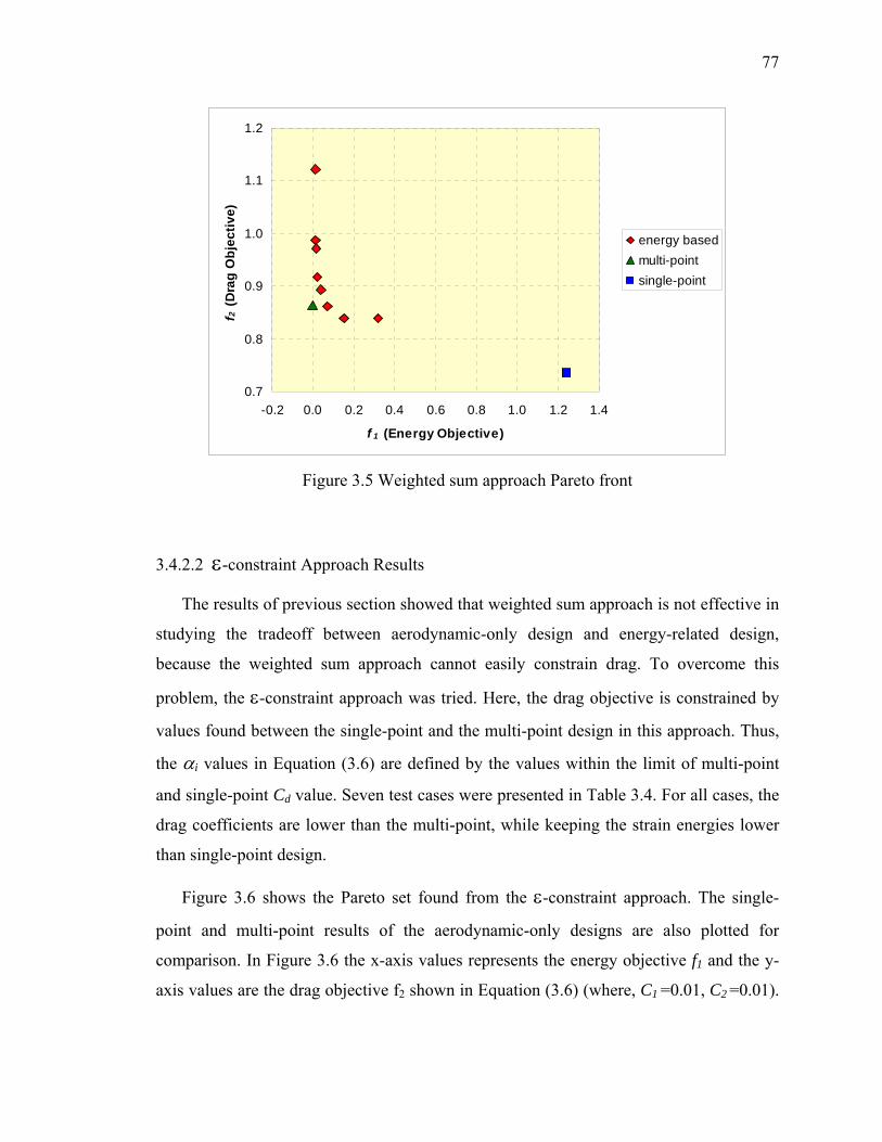
77
0.7
0.8
0.9
1.0
1.1
1.2
-0.2 0.0 0.2 0.4 0.6 0.8 1.0 1.2 1.4
f 1 (Energy Objective)
f 2 (D
rag
Obj
ectiv
e)energy basedmulti-pointsingle-point
Figure 3.5 Weighted sum approach Pareto front
3.4.2.2 ε-constraint Approach Results
The results of previous section showed that weighted sum approach is not effective in
studying the tradeoff between aerodynamic-only design and energy-related design,
because the weighted sum approach cannot easily constrain drag. To overcome this
problem, the ε-constraint approach was tried. Here, the drag objective is constrained by
values found between the single-point and the multi-point design in this approach. Thus,
the αi values in Equation (3.6) are defined by the values within the limit of multi-point
and single-point Cd value. Seven test cases were presented in Table 3.4. For all cases, the
drag coefficients are lower than the multi-point, while keeping the strain energies lower
than single-point design.
Figure 3.6 shows the Pareto set found from the ε-constraint approach. The single-
point and multi-point results of the aerodynamic-only designs are also plotted for
comparison. In Figure 3.6 the x-axis values represents the energy objective f1 and the y-
axis values are the drag objective f2 shown in Equation (3.6) (where, C1 =0.01, C2 =0.01).
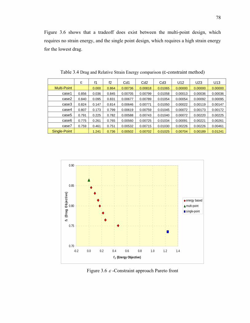
78
Figure 3.6 shows that a tradeoff does exist between the multi-point design, which
requires no strain energy, and the single point design, which requires a high strain energy
for the lowest drag.
Table 3.4 Drag and Relative Strain Energy comparison (ε-constraint method)
ε f1 f2 Cd1 Cd2 Cd3 U12 U23 U13 Multi-Point 0.000 0.864 0.00736 0.00818 0.01065 0.00000 0.00000 0.00000
case1 0.856 0.036 0.845 0.00705 0.00799 0.01058 0.00013 0.00036 0.00036 case2 0.840 0.095 0.831 0.00677 0.00789 0.01054 0.00054 0.00092 0.00095 case3 0.824 0.147 0.814 0.00646 0.00771 0.01050 0.00022 0.00119 0.00147 case4 0.807 0.173 0.799 0.00619 0.00759 0.01045 0.00072 0.00173 0.00172 case5 0.791 0.225 0.782 0.00588 0.00743 0.01040 0.00072 0.00220 0.00225 case6 0.775 0.261 0.765 0.00560 0.00725 0.01034 0.00091 0.00221 0.00261 case7 0.759 0.461 0.751 0.00532 0.00715 0.01030 0.00226 0.00226 0.00461
Single-Point 1.241 0.736 0.00502 0.00702 0.01025 0.00704 0.00189 0.01241
0.70
0.75
0.80
0.85
0.90
-0.2 0.0 0.2 0.4 0.6 0.8 1.0 1.2 1.4
f 1 (Energy Objective)
f 2 (D
rag
Obj
ectiv
e)
energy basedmulti-pointsingle-point
Figure 3.6 ε -Constraint approach Pareto front
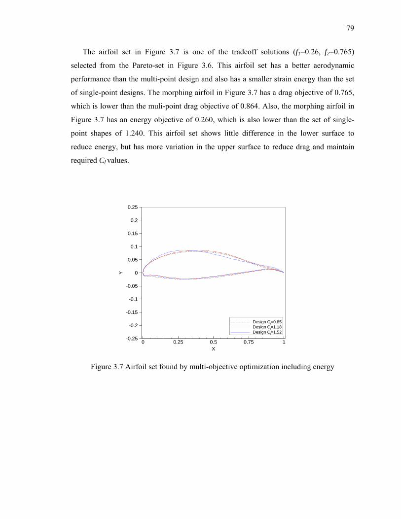
79
The airfoil set in Figure 3.7 is one of the tradeoff solutions (f1=0.26, f2=0.765)
selected from the Pareto-set in Figure 3.6. This airfoil set has a better aerodynamic
performance than the multi-point design and also has a smaller strain energy than the set
of single-point designs. The morphing airfoil in Figure 3.7 has a drag objective of 0.765,
which is lower than the muli-point drag objective of 0.864. Also, the morphing airfoil in
Figure 3.7 has an energy objective of 0.260, which is also lower than the set of single-
point shapes of 1.240. This airfoil set shows little difference in the lower surface to
reduce energy, but has more variation in the upper surface to reduce drag and maintain
required Cl values.
0 0.25 0.5 0.75 1X
-0.25
-0.2
-0.15
-0.1
-0.05
0
0.05
0.1
0.15
0.2
0.25
Y
Design Cl=0.85Design Cl=1.18Design Cl=1.52
Figure 3.7 Airfoil set found by multi-objective optimization including energy
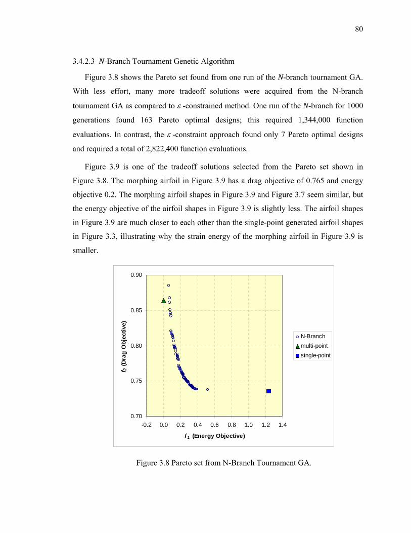
80
3.4.2.3 N-Branch Tournament Genetic Algorithm
Figure 3.8 shows the Pareto set found from one run of the N-branch tournament GA.
With less effort, many more tradeoff solutions were acquired from the N-branch
tournament GA as compared to ε -constrained method. One run of the N-branch for 1000
generations found 163 Pareto optimal designs; this required 1,344,000 function
evaluations. In contrast, the ε -constraint approach found only 7 Pareto optimal designs
and required a total of 2,822,400 function evaluations.
Figure 3.9 is one of the tradeoff solutions selected from the Pareto set shown in
Figure 3.8. The morphing airfoil in Figure 3.9 has a drag objective of 0.765 and energy
objective 0.2. The morphing airfoil shapes in Figure 3.9 and Figure 3.7 seem similar, but
the energy objective of the airfoil shapes in Figure 3.9 is slightly less. The airfoil shapes
in Figure 3.9 are much closer to each other than the single-point generated airfoil shapes
in Figure 3.3, illustrating why the strain energy of the morphing airfoil in Figure 3.9 is
smaller.
0.70
0.75
0.80
0.85
0.90
-0.2 0.0 0.2 0.4 0.6 0.8 1.0 1.2 1.4
f 1 (Energy Objective)
f 2 (D
rag
Obj
ectiv
e)
N-Branchmulti-pointsingle-point
Figure 3.8 Pareto set from N-Branch Tournament GA.
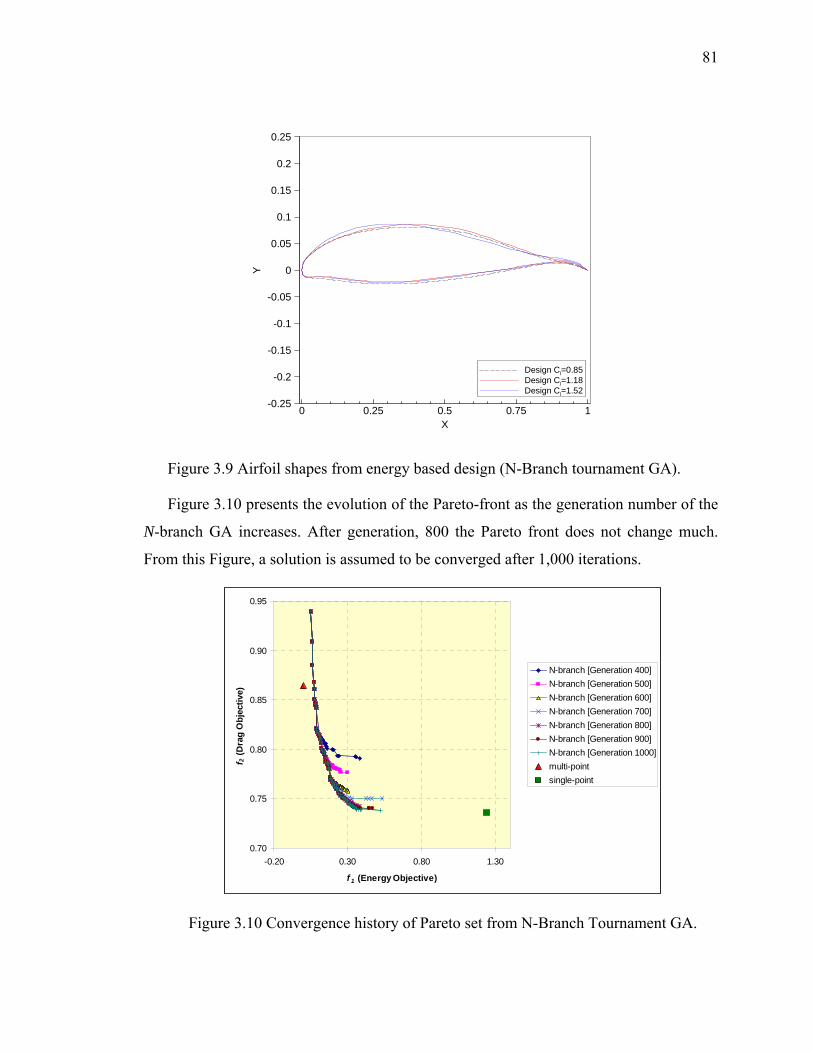
81
0 0.25 0.5 0.75 1X
-0.25
-0.2
-0.15
-0.1
-0.05
0
0.05
0.1
0.15
0.2
0.25
Y
Design Cl=0.85Design Cl=1.18Design Cl=1.52
Figure 3.9 Airfoil shapes from energy based design (N-Branch tournament GA).
Figure 3.10 presents the evolution of the Pareto-front as the generation number of the
N-branch GA increases. After generation, 800 the Pareto front does not change much.
From this Figure, a solution is assumed to be converged after 1,000 iterations.
0.70
0.75
0.80
0.85
0.90
0.95
-0.20 0.30 0.80 1.30
f 1 (Energy Objective)
f 2 (D
rag
Obj
ectiv
e)
N-branch [Generation 400]N-branch [Generation 500]N-branch [Generation 600]N-branch [Generation 700]N-branch [Generation 800]N-branch [Generation 900]N-branch [Generation 1000]multi-pointsingle-point
Figure 3.10 Convergence history of Pareto set from N-Branch Tournament GA.
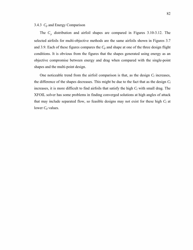
82
3.4.3 Cp and Energy Comparison
The pC distribution and airfoil shapes are compared in Figures 3.10-3.12. The
selected airfoils for multi-objective methods are the same airfoils shown in Figures 3.7
and 3.9. Each of these figures compares the Cp and shape at one of the three design flight
conditions. It is obvious from the figures that the shapes generated using energy as an
objective compromise between energy and drag when compared with the single-point
shapes and the multi-point design.
One noticeable trend from the airfoil comparison is that, as the design Cl increases,
the difference of the shapes decreases. This might be due to the fact that as the design Cl
increases, it is more difficult to find airfoils that satisfy the high Cl with small drag. The
XFOIL solver has some problems in finding converged solutions at high angles of attack
that may include separated flow, so feasible designs may not exist for these high Cl at
lower Cd values.
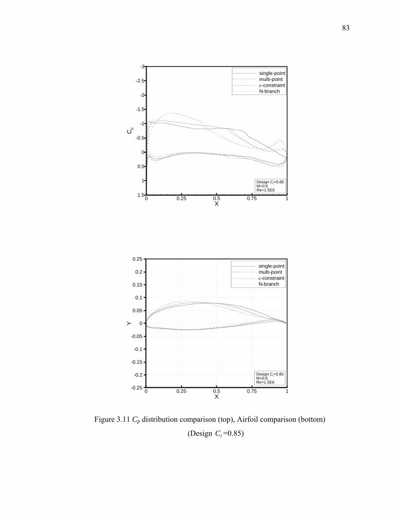
83
0 0.25 0.5 0.75 1X
-3
-2.5
-2
-1.5
-1
-0.5
0
0.5
1
1.5
Cp
single-pointmulti-pointε-constraintN-branch
Design Cl=0.85M=0.6Re=1.5E6
0 0.25 0.5 0.75 1X
-0.25
-0.2
-0.15
-0.1
-0.05
0
0.05
0.1
0.15
0.2
0.25
Y
single-pointmulti-pointε-constraintN-branch
Design Cl=0.85M=0.6Re=1.5E6
Figure 3.11 Cp distribution comparison (top), Airfoil comparison (bottom)
(Design lC =0.85)
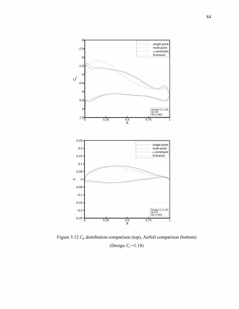
84
0 0.25 0.5 0.75 1X
-3
-2.5
-2
-1.5
-1
-0.5
0
0.5
1
1.5
Cp
single-pointmulti-pointε-constraintN-branch
Design Cl=1.18M=0.6Re=1.5E6
0 0.25 0.5 0.75 1X
-0.25
-0.2
-0.15
-0.1
-0.05
0
0.05
0.1
0.15
0.2
0.25
Y
single-pointmulti-pointε-constraintN-branch
Design Cl=1.18M=0.6Re=1.5E6
Figure 3.12 Cp distribution comparison (top), Airfoil comparison (bottom)
(Design lC =1.18)
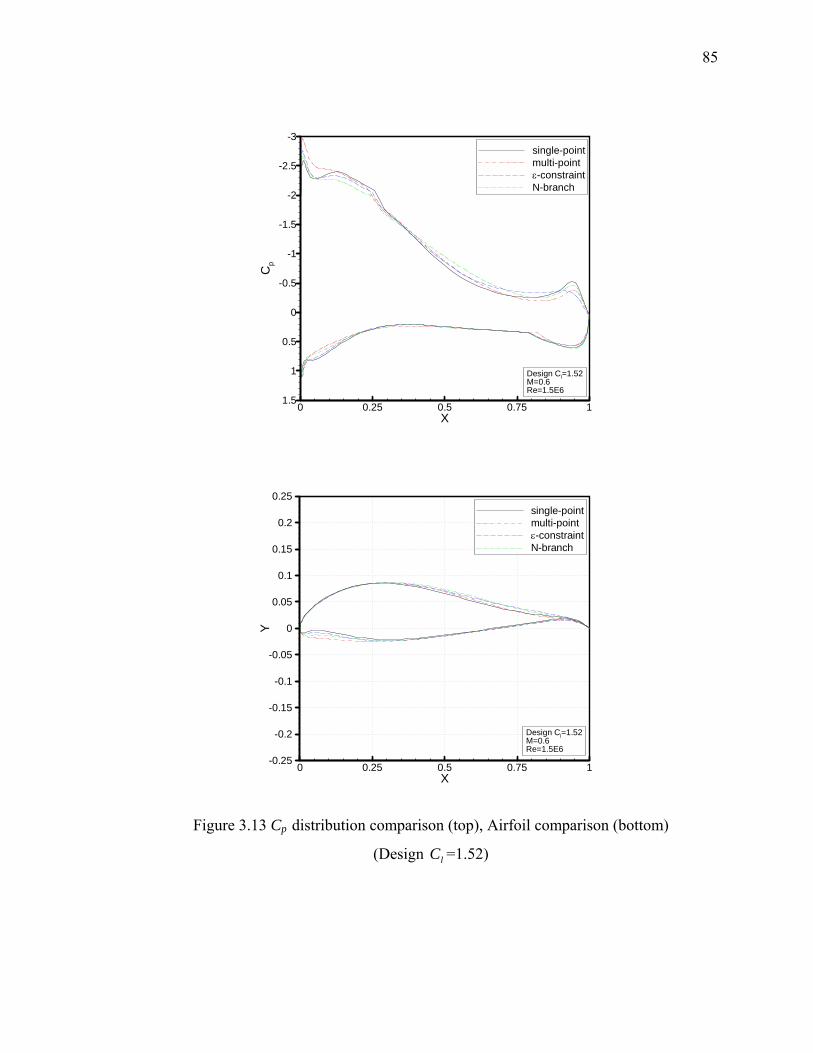
85
0 0.25 0.5 0.75 1X
-3
-2.5
-2
-1.5
-1
-0.5
0
0.5
1
1.5
Cp
single-pointmulti-pointε-constraintN-branch
Design Cl=1.52M=0.6Re=1.5E6
0 0.25 0.5 0.75 1X
-0.25
-0.2
-0.15
-0.1
-0.05
0
0.05
0.1
0.15
0.2
0.25
Y
single-pointmulti-pointε-constraintN-branch
Design Cl=1.52M=0.6Re=1.5E6
Figure 3.13 Cp distribution comparison (top), Airfoil comparison (bottom)
(Design lC =1.52)
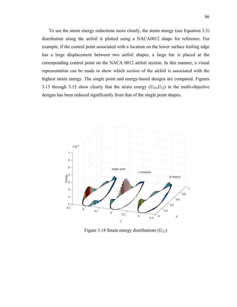
86
To see the strain energy reductions more clearly, the strain energy (see Equation 3.3)
distribution along the airfoil is plotted using a NACA0012 shape for reference. For
example, if the control point associated with a location on the lower surface trailing edge
has a large displacement between two airfoil shapes, a large bar is placed at the
corresponding control point on the NACA 0012 airfoil section. In this manner, a visual
representation can be made to show which section of the airfoil is associated with the
highest strain energy. The single point and energy-based designs are compared. Figures
3.13 through 3.15 show clearly that the strain energy (U23,U13) in the multi-objective
designs has been reduced significantly from that of the single point shapes.
0
0.2
0.4
0.6
0.8
1
0.10
0.10
0.10
0.10
1
2
3
4
5
6
7
x 10−4
X
y
Ene
rgy
single−point ε−constraint
N−branch
Figure 3.14 Strain energy distributions (U12)
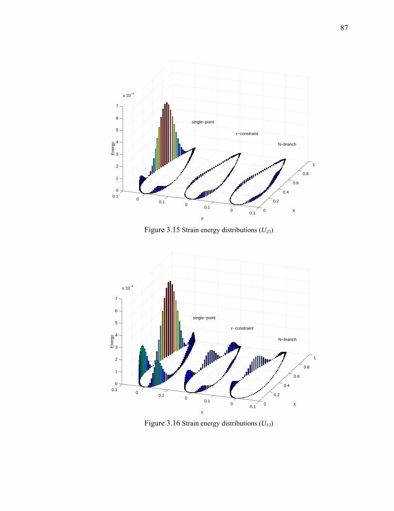
87
0
0.2
0.4
0.6
0.8
1
0.10
0.10
0.10
0.1 0
1
2
3
4
5
6
7
x 10−4
X
y
Ene
rgy
single−point
ε−constraint
N−branch
Figure 3.15 Strain energy distributions (U23)
0
0.2
0.4
0.6
0.8
1
0.10
0.10
0.10
0.1 0
1
2
3
4
5
6
7
x 10−4
X
y
Ene
rgy
single−point
ε−constraint
N−branch
Figure 3.16 Strain energy distributions (U13)
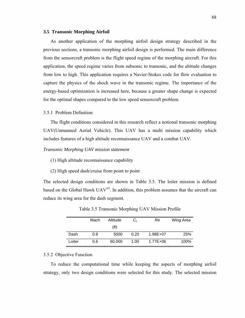
88
3.5 Transonic Morphing Airfoil
As another application of the morphing airfoil design strategy described in the
previous sections, a transonic morphing airfoil design is performed. The main difference
from the sensorcraft problem is the flight speed regime of the morphing aircraft. For this
application, the speed regime varies from subsonic to transonic, and the altitude changes
from low to high. This application requires a Navier-Stokes code for flow evaluation to
capture the physics of the shock wave in the transonic regime. The importance of the
energy-based optimization is increased here, because a greater shape change is expected
for the optimal shapes compared to the low speed sensorcraft problem.
3.5.1 Problem Definition
The flight conditions considered in this research reflect a notional transonic morphing
UAV(Unmanned Aerial Vehicle). This UAV has a multi mission capability which
includes features of a high altitude reconnaissance UAV and a combat UAV.
Transonic Morphing UAV mission statement
(1) High altitude reconnaissance capability
(2) High speed dash/cruise from point to point
The selected design conditions are shown in Table 3.5. The loiter mission is defined
based on the Global Hawk UAV65. In addition, this problem assumes that the aircraft can
reduce its wing area for the dash segment.
Table 3.5 Transonic Morphing UAV Mission Profile
Mach Altitude
(ft)
CL Re Wing Area
Dash 0.8 5000 0.20 1.98E+07 25%
Loiter 0.6 60,000 1.00 1.77E+06 100%
3.5.2 Objective Function
To reduce the computational time while keeping the aspects of morphing airfoil
strategy, only two design conditions were selected for this study. The selected mission
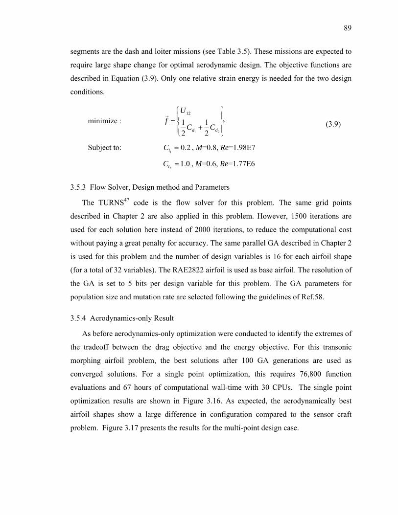
89
segments are the dash and loiter missions (see Table 3.5). These missions are expected to
require large shape change for optimal aerodynamic design. The objective functions are
described in Equation (3.9). Only one relative strain energy is needed for the two design
conditions.
minimize : ⎪⎭
⎪⎬⎫
⎪⎩
⎪⎨⎧
+=
21 21
21
12
dd CC
Uf
Subject to: 2.01
=lC , M=0.8, Re=1.98E7
0.12
=lC , M=0.6, Re=1.77E6
(3.9)
3.5.3 Flow Solver, Design method and Parameters
The TURNS47 code is the flow solver for this problem. The same grid points
described in Chapter 2 are also applied in this problem. However, 1500 iterations are
used for each solution here instead of 2000 iterations, to reduce the computational cost
without paying a great penalty for accuracy. The same parallel GA described in Chapter 2
is used for this problem and the number of design variables is 16 for each airfoil shape
(for a total of 32 variables). The RAE2822 airfoil is used as base airfoil. The resolution of
the GA is set to 5 bits per design variable for this problem. The GA parameters for
population size and mutation rate are selected following the guidelines of Ref.58.
3.5.4 Aerodynamics-only Result
As before aerodynamics-only optimization were conducted to identify the extremes of
the tradeoff between the drag objective and the energy objective. For this transonic
morphing airfoil problem, the best solutions after 100 GA generations are used as
converged solutions. For a single point optimization, this requires 76,800 function
evaluations and 67 hours of computational wall-time with 30 CPUs. The single point
optimization results are shown in Figure 3.16. As expected, the aerodynamically best
airfoil shapes show a large difference in configuration compared to the sensor craft
problem. Figure 3.17 presents the results for the multi-point design case.
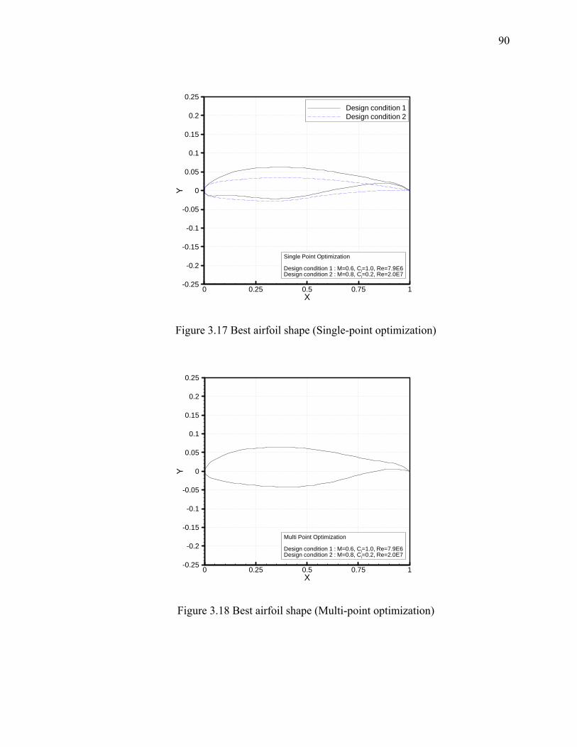
90
0 0.25 0.5 0.75 1X
-0.25
-0.2
-0.15
-0.1
-0.05
0
0.05
0.1
0.15
0.2
0.25
Y
Design condition 1Design condition 2
Single Point Optimization
Design condition 1 : M=0.6, Cl=1.0, Re=7.9E6Design condition 2 : M=0.8, Cl=0.2, Re=2.0E7
Figure 3.17 Best airfoil shape (Single-point optimization)
0 0.25 0.5 0.75 1X
-0.25
-0.2
-0.15
-0.1
-0.05
0
0.05
0.1
0.15
0.2
0.25
Y
Multi Point Optimization
Design condition 1 : M=0.6, Cl=1.0, Re=7.9E6Design condition 2 : M=0.8, Cl=0.2, Re=2.0E7
Figure 3.18 Best airfoil shape (Multi-point optimization)
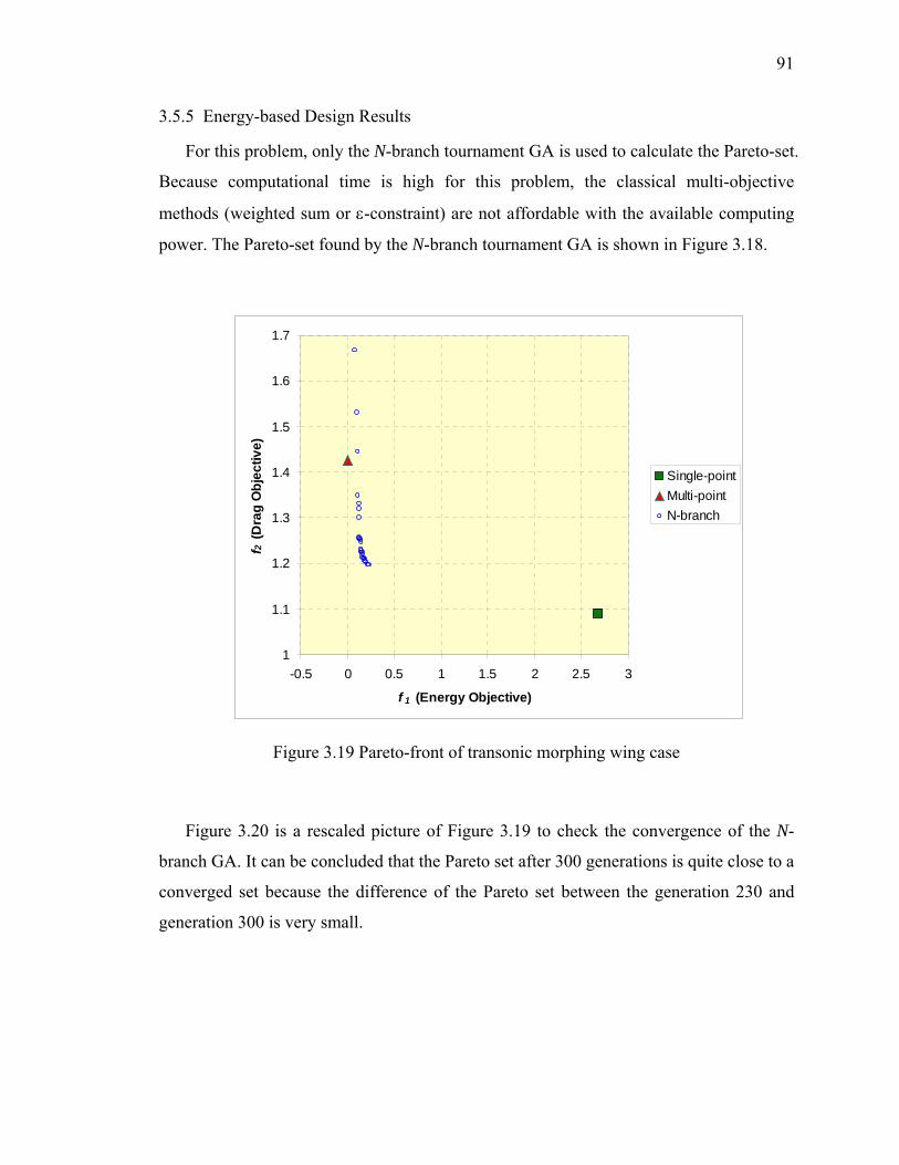
91
3.5.5 Energy-based Design Results
For this problem, only the N-branch tournament GA is used to calculate the Pareto-set.
Because computational time is high for this problem, the classical multi-objective
methods (weighted sum or ε-constraint) are not affordable with the available computing
power. The Pareto-set found by the N-branch tournament GA is shown in Figure 3.18.
1
1.1
1.2
1.3
1.4
1.5
1.6
1.7
-0.5 0 0.5 1 1.5 2 2.5 3
f 1 (Energy Objective)
f 2 (D
rag
Obj
ectiv
e)
Single-pointMulti-pointN-branch
Figure 3.19 Pareto-front of transonic morphing wing case
Figure 3.20 is a rescaled picture of Figure 3.19 to check the convergence of the N-
branch GA. It can be concluded that the Pareto set after 300 generations is quite close to a
converged set because the difference of the Pareto set between the generation 230 and
generation 300 is very small.
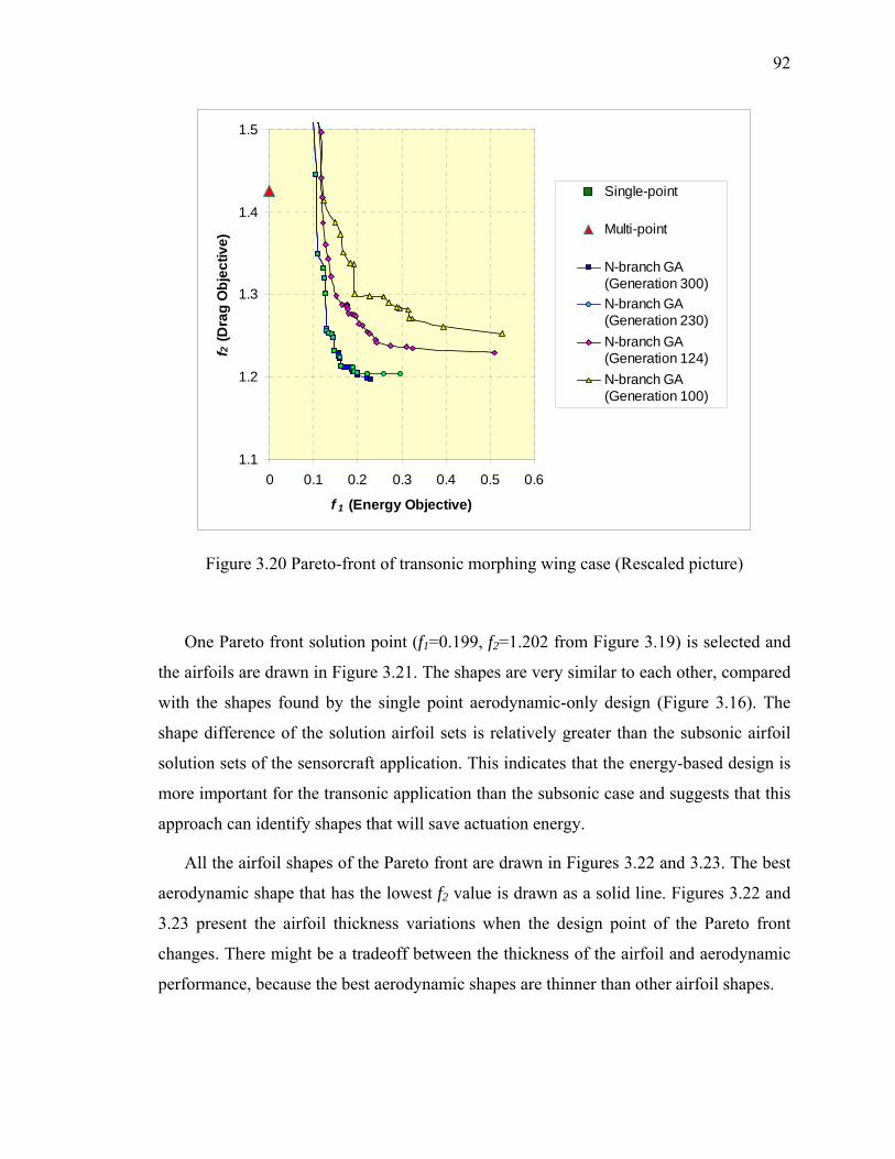
92
1.1
1.2
1.3
1.4
1.5
0 0.1 0.2 0.3 0.4 0.5 0.6
f 1 (Energy Objective)
f 2 (D
rag
Obj
ectiv
e)
Single-point
Multi-point
N-branch GA(Generation 300)N-branch GA(Generation 230)N-branch GA(Generation 124)N-branch GA(Generation 100)
Figure 3.20 Pareto-front of transonic morphing wing case (Rescaled picture)
One Pareto front solution point (f1=0.199, f2=1.202 from Figure 3.19) is selected and
the airfoils are drawn in Figure 3.21. The shapes are very similar to each other, compared
with the shapes found by the single point aerodynamic-only design (Figure 3.16). The
shape difference of the solution airfoil sets is relatively greater than the subsonic airfoil
solution sets of the sensorcraft application. This indicates that the energy-based design is
more important for the transonic application than the subsonic case and suggests that this
approach can identify shapes that will save actuation energy.
All the airfoil shapes of the Pareto front are drawn in Figures 3.22 and 3.23. The best
aerodynamic shape that has the lowest f2 value is drawn as a solid line. Figures 3.22 and
3.23 present the airfoil thickness variations when the design point of the Pareto front
changes. There might be a tradeoff between the thickness of the airfoil and aerodynamic
performance, because the best aerodynamic shapes are thinner than other airfoil shapes.
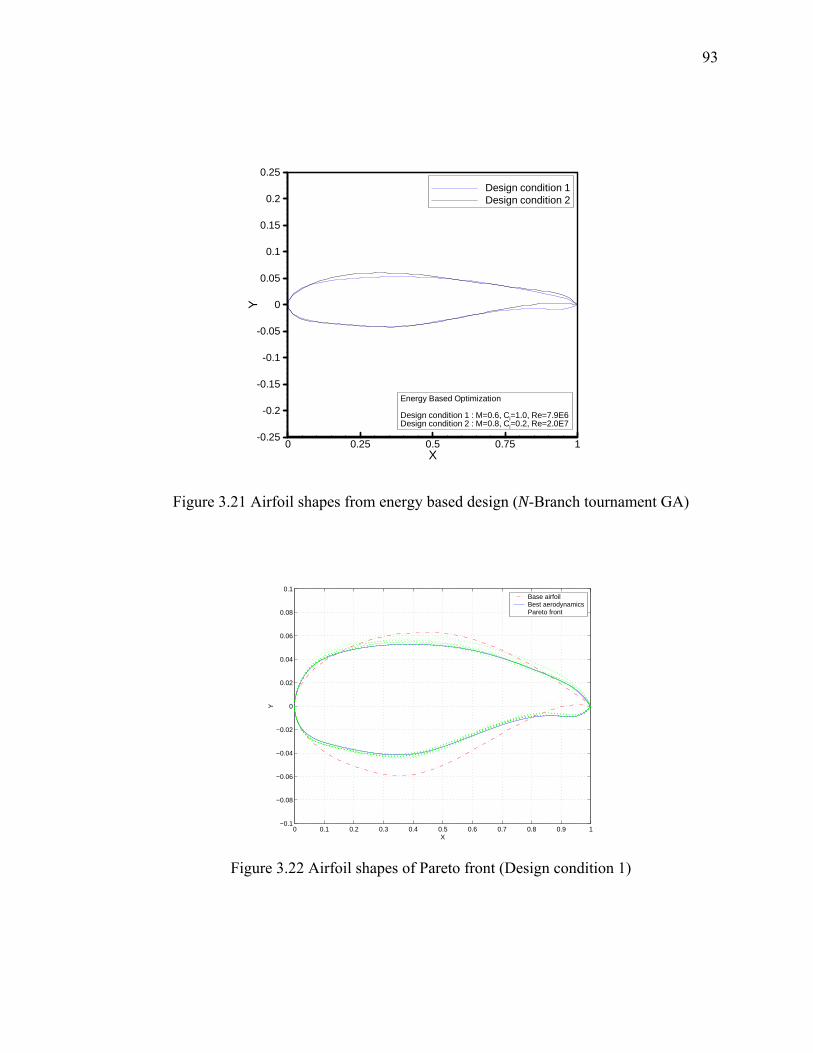
93
0 0.25 0.5 0.75 1X
-0.25
-0.2
-0.15
-0.1
-0.05
0
0.05
0.1
0.15
0.2
0.25
Y
Design condition 1Design condition 2
Energy Based Optimization
Design condition 1 : M=0.6, Cl=1.0, Re=7.9E6Design condition 2 : M=0.8, Cl=0.2, Re=2.0E7
Figure 3.21 Airfoil shapes from energy based design (N-Branch tournament GA)
0 0.1 0.2 0.3 0.4 0.5 0.6 0.7 0.8 0.9 1−0.1
−0.08
−0.06
−0.04
−0.02
0
0.02
0.04
0.06
0.08
0.1
X
Y
Base airfoilBest aerodynamicsPareto front
Figure 3.22 Airfoil shapes of Pareto front (Design condition 1)
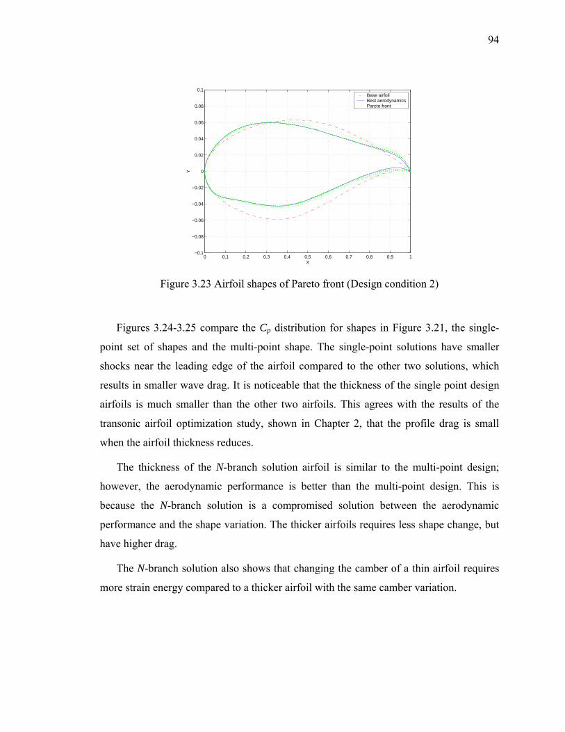
94
0 0.1 0.2 0.3 0.4 0.5 0.6 0.7 0.8 0.9 1−0.1
−0.08
−0.06
−0.04
−0.02
0
0.02
0.04
0.06
0.08
0.1
X
Y
Base airfoilBest aerodynamicsPareto front
Figure 3.23 Airfoil shapes of Pareto front (Design condition 2)
Figures 3.24-3.25 compare the Cp distribution for shapes in Figure 3.21, the single-
point set of shapes and the multi-point shape. The single-point solutions have smaller
shocks near the leading edge of the airfoil compared to the other two solutions, which
results in smaller wave drag. It is noticeable that the thickness of the single point design
airfoils is much smaller than the other two airfoils. This agrees with the results of the
transonic airfoil optimization study, shown in Chapter 2, that the profile drag is small
when the airfoil thickness reduces.
The thickness of the N-branch solution airfoil is similar to the multi-point design;
however, the aerodynamic performance is better than the multi-point design. This is
because the N-branch solution is a compromised solution between the aerodynamic
performance and the shape variation. The thicker airfoils requires less shape change, but
have higher drag.
The N-branch solution also shows that changing the camber of a thin airfoil requires
more strain energy compared to a thicker airfoil with the same camber variation.
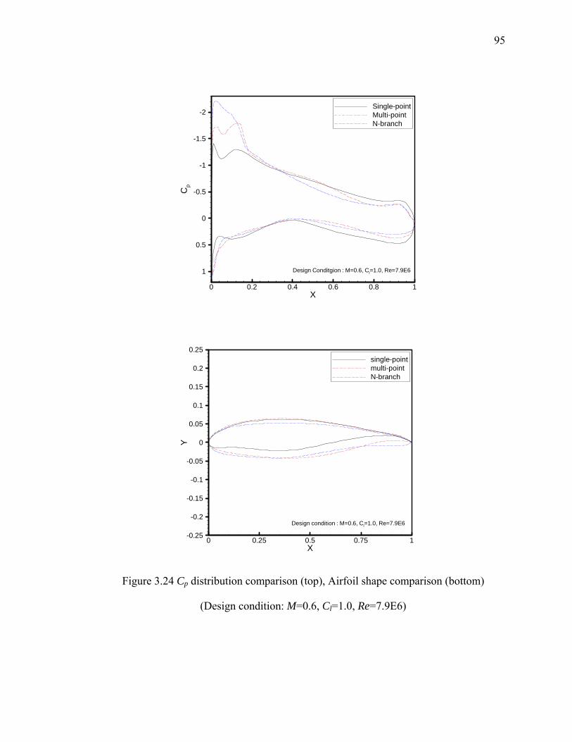
95
0 0.2 0.4 0.6 0.8 1X
-2
-1.5
-1
-0.5
0
0.5
1
Cp
Single-pointMulti-pointN-branch
Design Conditgion : M=0.6, Cl=1.0, Re=7.9E6
0 0.25 0.5 0.75 1X
-0.25
-0.2
-0.15
-0.1
-0.05
0
0.05
0.1
0.15
0.2
0.25
Y
single-pointmulti-pointN-branch
Design condition : M=0.6, Cl=1.0, Re=7.9E6
Figure 3.24 Cp distribution comparison (top), Airfoil shape comparison (bottom)
(Design condition: M=0.6, Cl=1.0, Re=7.9E6)
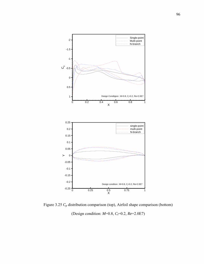
96
0 0.2 0.4 0.6 0.8 1X
-2
-1.5
-1
-0.5
0
0.5
1
Cp
Single-pointMulti-pointN-branch
Design Conditgion : M=0.8, Cl=0.2, Re=2.0E7
0 0.25 0.5 0.75 1X
-0.25
-0.2
-0.15
-0.1
-0.05
0
0.05
0.1
0.15
0.2
0.25
Y
single-pointmulti-pointN-branch
Design condition : M=0.8, Cl=0.2, Re=2.0E7
Figure 3.25 Cp distribution comparison (top), Airfoil shape comparison (bottom)
(Design condition: M=0.8, Cl=0.2, Re=2.0E7)
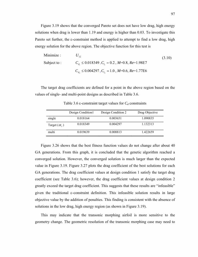
97
Figure 3.19 shows that the converged Pareto set does not have low drag, high energy
solutions when drag is lower than 1.19 and energy is higher than 0.03. To investigate this
Pareto set further, the ε-constraint method is applied to attempt to find a low drag, high
energy solution for the above region. The objective function for this test is
Minimize : 12U
Subject to : 018349.01
≤dC , 2.01
=lC , M=0.8, Re=1.98E7
004297.02
≤dC , 0.12
=lC , M=0.6, Re=1.77E6
(3.10)
The target drag coefficients are defined for a point in the above region based on the
values of single- and multi-point designs as described in Table 3.6.
Table 3.6 ε-constraint target values for Cd constraints
Design Condition1 Design Condition 2 Drag Objective
single 0.018164 0.003651 1.090835
Target ( iα ) 0.018349 0.004297 1.132313
multi 0.019639 0.008813 1.422659
Figure 3.26 shows that the best fitness function values do not change after about 40
GA generations. From this graph, it is concluded that the genetic algorithm reached a
converged solution. However, the converged solution is much larger than the expected
value in Figure 3.19. Figure 3.27 plots the drag coefficient of the best solutions for each
GA generations. The drag coefficient values at design condition 1 satisfy the target drag
coefficient (see Table 3.6); however, the drag coefficient values at design condition 2
greatly exceed the target drag coefficient. This suggests that these results are “infeasible”
given the traditional ε-constraint definition. This infeasible solution results in large
objective value by the addition of penalties. This finding is consistent with the absence of
solutions in the low drag, high energy region (as shown in Figure 3.19).
This may indicate that the transonic morphing airfoil is more sensitive to the
geometry change. The geometric resolution of the transonic morphing case may need to

98
be increased (e.g. finer resolution between discretized design variable values) to find
feasible solutions with low drag and low energy. This increase of geometric resolution
will require a larger computational effort, because the chromosome length and population
size would also need to increase significantly.
-450
-400
-350
-300
-250
-200
1 11 21 31 41 51 61 71 81 91Generations
Fitn
ess
func
tion
valu
e
Figure 3.26 GA convergence history of ε-constraint method
0
0.005
0.01
0.015
0.02
0.025
0.03
1 11 21 31 41 51 61 71 81 91
Generation
Dra
g co
effic
ient
Cd 1(M=0.6,Cl=1.0,Re=1.7E6)Cd 2(M=0.8,Cl=0.2,Re=2.0E7)
Figure 3.27 Drag coefficient values
99
3.6 Summary
The multi-objective optimization approach is applied for the morphing airfoil design
problem instead of the single-objective approach. The two objectives are minimization of
drag and morphing energy. Three different multi-objective optimization methods have
been chosen and the results are compared.
To calculate the energy objective for multi-point design conditions, the maximum
value is used instead of a weighted summation of the relative strain energy values. This is
because the actuator needs to be big enough to overcome the maximum actuation load.
The sensorcraft problem showed that minimizing the drag objective is more difficult
compared to minimizing the strain energy objective. Because of this, the weighted sum
approach is not appropriate for this problem, but the ε-constraint method and N-branch
tournament method do work for the sensorcraft problem. The N-branch tournament
method result showed that this method is very efficient in finding tradeoff solutions
compare to the ε-constraint method, because it could acquire more Pareto-front solutions
with one single run of GA.
As a second application of the morphing airfoil design strategy, transonic morphing
airfoils are designed. For the transonic example, a difference of the optimal shape for the
design conditions is greater than the subsonic case. This increases the importance of the
energy-based design strategy for transonic morphing airfoil design. There were no low
drag and low energy designs found by N-branch GA for transonic morphing airfoil and
this appears to be the result of low geometric resolution of the possible airfoil sets.
100
CHAPTER 4 ACTUATION ENERGY MODELING INCLUDING
AERODYNAMIC WORK
4.1 Description of Concept
The morphing airfoil design strategy described in the previous chapter does not
account for the effect of the external air load on the airfoil shape. If the structure of the
wing is very stiff so that deformation caused by the external aerodynamic load can be
ignored, then this assumption is quite appropriate. However, for a morphing aircraft, the
aerodynamic load should not be ignored, because the shape change requires a flexible
wing.
The pressure distribution acting on an airfoil can be represented by a series of forces
acting at specific control points on the airfoil. The direction and magnitude of these
forces depend on both the flight condition and the local shape of the airfoil. Figure 4.1
displays two airfoils, each designed to minimize drag at a different lift coefficient. The
aerodynamic forces acting on the airfoil are presented as vectors, and the two plots show
that if the airfoil shape and flight conditions change, the aerodynamic force distribution
also changes. Because the goal of the morphing airfoil is to change the shape of the
airfoil, there is a possibility to acquire some assist from the aerodynamic force, or the
possibility that the actuation effort needs to increase to overcome the aerodynamic force
and the structural stiffness.
Figure 4.2 illustrates how the variation in airfoil shape change impacts the direction
and magnitude of the aerodynamic forces. This, in turn, can affect the required effort
from the morphing actuators. In Figure 4.2, two exaggerated airfoil shapes are shown; the
black dashed shape represents the initial shape and the blue solid shape represents the
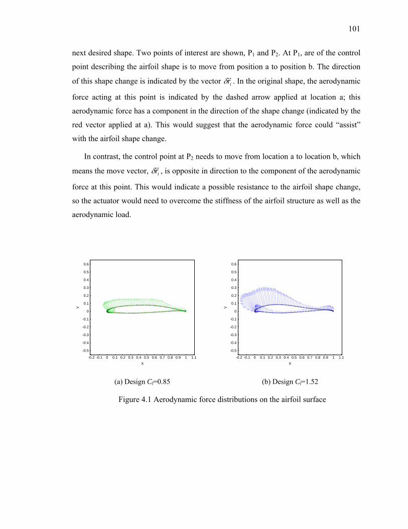
101
next desired shape. Two points of interest are shown, P1 and P2. At P1, are of the control
point describing the airfoil shape is to move from position a to position b. The direction
of this shape change is indicated by the vector irδ . In the original shape, the aerodynamic
force acting at this point is indicated by the dashed arrow applied at location a; this
aerodynamic force has a component in the direction of the shape change (indicated by the
red vector applied at a). This would suggest that the aerodynamic force could “assist”
with the airfoil shape change.
In contrast, the control point at P2 needs to move from location a to location b, which
means the move vector, irδ , is opposite in direction to the component of the aerodynamic
force at this point. This would indicate a possible resistance to the airfoil shape change,
so the actuator would need to overcome the stiffness of the airfoil structure as well as the
aerodynamic load.
-0.2 -0.1 0 0.1 0.2 0.3 0.4 0.5 0.6 0.7 0.8 0.9 1 1.1X
-0.5
-0.4
-0.3
-0.2
-0.1
0
0.1
0.2
0.3
0.4
0.5
0.6
Y
-0.2 -0.1 0 0.1 0.2 0.3 0.4 0.5 0.6 0.7 0.8 0.9 1 1.1
X
-0.5
-0.4
-0.3
-0.2
-0.1
0
0.1
0.2
0.3
0.4
0.5
0.6
Y
(a) Design Cl=0.85 (b) Design Cl=1.52
Figure 4.1 Aerodynamic force distributions on the airfoil surface
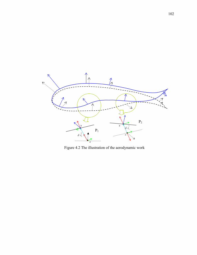
102
Figure 4.2 The illustration of the aerodynamic work
→
irδ
→
irδ
a
b b
a
P1
P2
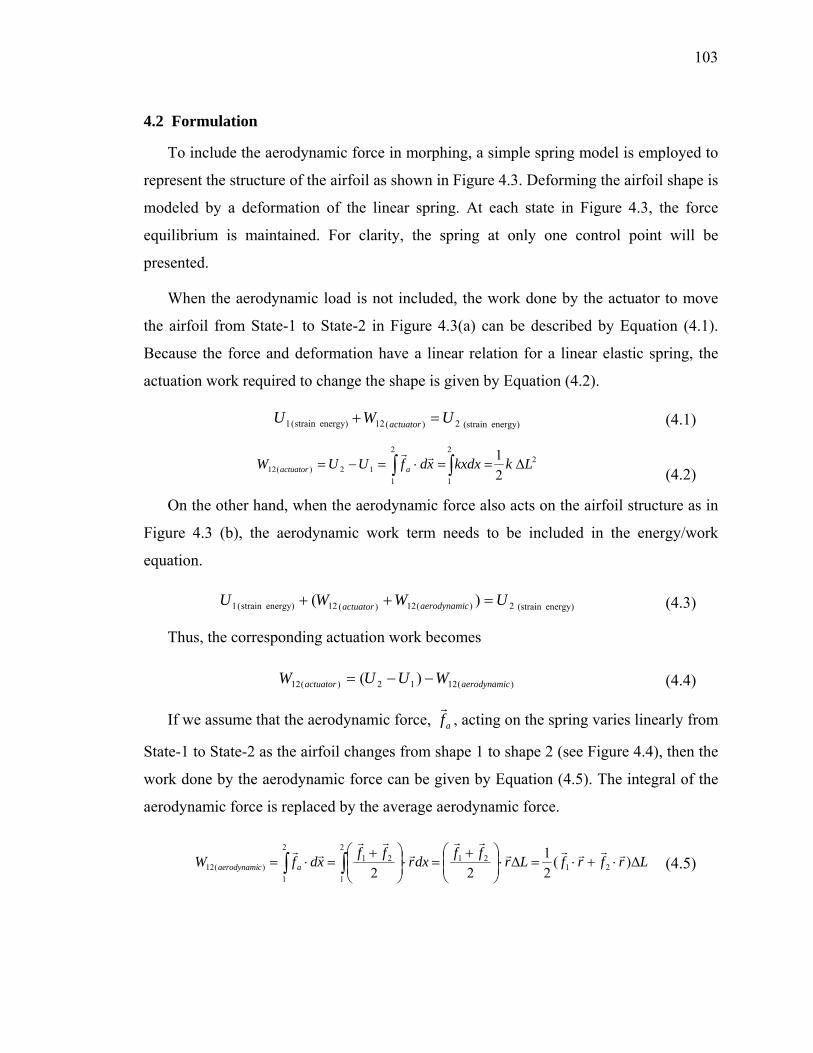
103
4.2 Formulation
To include the aerodynamic force in morphing, a simple spring model is employed to
represent the structure of the airfoil as shown in Figure 4.3. Deforming the airfoil shape is
modeled by a deformation of the linear spring. At each state in Figure 4.3, the force
equilibrium is maintained. For clarity, the spring at only one control point will be
presented.
When the aerodynamic load is not included, the work done by the actuator to move
the airfoil from State-1 to State-2 in Figure 4.3(a) can be described by Equation (4.1).
Because the force and deformation have a linear relation for a linear elastic spring, the
actuation work required to change the shape is given by Equation (4.2).
energy)(strain 2)(12energy)strain ( 1 UWU actuator =+
22
1
2
112)(12
21 LkkxdxxdfUUW aactuator Δ==⋅=−= ∫∫
(4.1)
(4.2)
On the other hand, when the aerodynamic force also acts on the airfoil structure as in
Figure 4.3 (b), the aerodynamic work term needs to be included in the energy/work
equation.
energy)(strain 2)(12)(12energy)strain ( 1 )( UWWU caerodynamiactuator =++ (4.3)
Thus, the corresponding actuation work becomes
)(1212)(12 )( caerodynamiactuator WUUW −−= (4.4)
If we assume that the aerodynamic force, af , acting on the spring varies linearly from
State-1 to State-2 as the airfoil changes from shape 1 to shape 2 (see Figure 4.4), then the
work done by the aerodynamic force can be given by Equation (4.5). The integral of the
aerodynamic force is replaced by the average aerodynamic force.
LrfrfLrffdxrffxdfW acaerodynami Δ⋅+⋅=Δ⋅⎟⎟⎠
⎞⎜⎜⎝
⎛ +=⋅⎟⎟
⎠
⎞⎜⎜⎝
⎛ +=⋅= ∫ ∫ )(
21
22 2121
2
1
2
1
21)(12
(4.5)
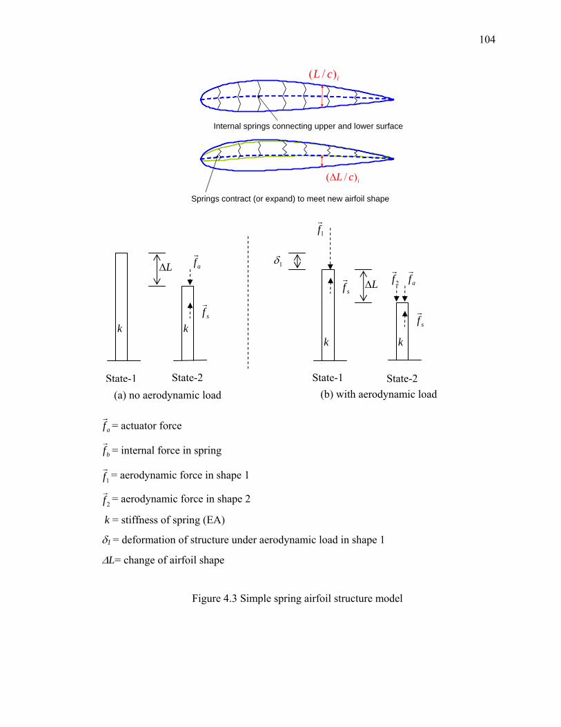
104
Internal springs connecting upper and lower surface
icL )/(Δ
icL )/(
Springs contract (or expand) to meet new airfoil shape
af = actuator force
bf = internal force in spring
1f = aerodynamic force in shape 1
2f = aerodynamic force in shape 2
k = stiffness of spring (EA)
δ1 = deformation of structure under aerodynamic load in shape 1
ΔL= change of airfoil shape
Figure 4.3 Simple spring airfoil structure model
LΔ
LΔ
1δ
1f
2f afaf
k kk k
State-1 State-2 (b) with aerodynamic load
sfsf
sf
State-2 State-1(a) no aerodynamic load
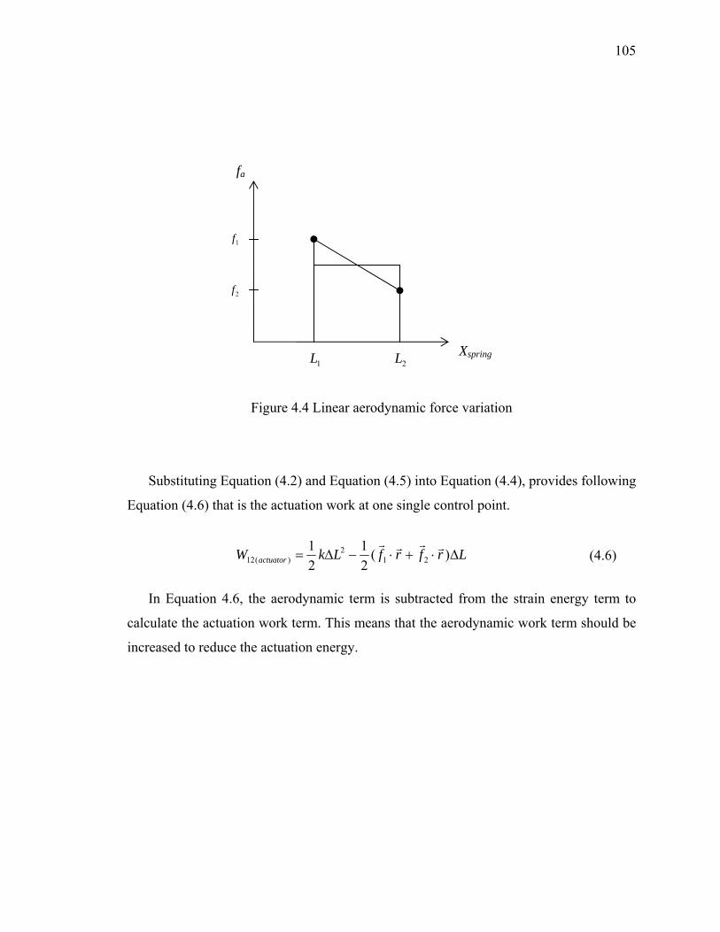
105
Figure 4.4 Linear aerodynamic force variation
Substituting Equation (4.2) and Equation (4.5) into Equation (4.4), provides following
Equation (4.6) that is the actuation work at one single control point.
LrfrfLkW actuator Δ⋅+⋅−Δ= )(21
21
212
)(12 (4.6)
In Equation 4.6, the aerodynamic term is subtracted from the strain energy term to
calculate the actuation work term. This means that the aerodynamic work term should be
increased to reduce the actuation energy.
Xspring
2f
1f
1L 2L
fa
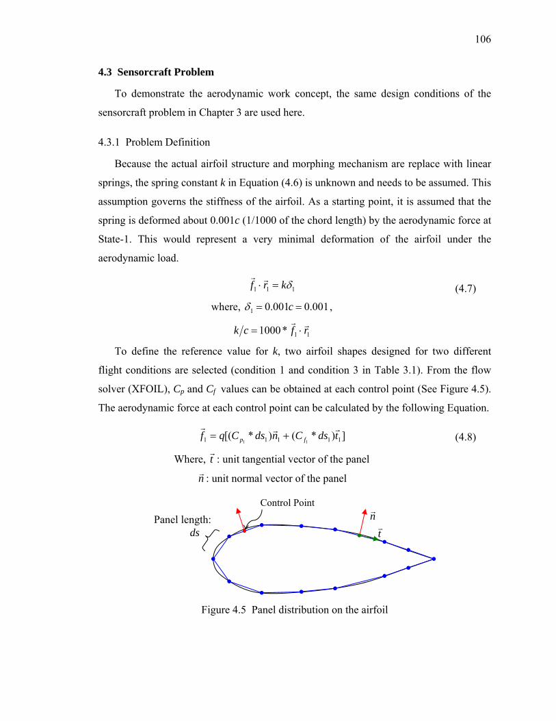
106
4.3 Sensorcraft Problem
To demonstrate the aerodynamic work concept, the same design conditions of the
sensorcraft problem in Chapter 3 are used here.
4.3.1 Problem Definition
Because the actual airfoil structure and morphing mechanism are replace with linear
springs, the spring constant k in Equation (4.6) is unknown and needs to be assumed. This
assumption governs the stiffness of the airfoil. As a starting point, it is assumed that the
spring is deformed about 0.001c (1/1000 of the chord length) by the aerodynamic force at
State-1. This would represent a very minimal deformation of the airfoil under the
aerodynamic load.
111 δkrf =⋅
where, 001.0001.01 == cδ ,
11*1000 rfck ⋅=
(4.7)
To define the reference value for k, two airfoil shapes designed for two different
flight conditions are selected (condition 1 and condition 3 in Table 3.1). From the flow
solver (XFOIL), Cp and Cf values can be obtained at each control point (See Figure 4.5).
The aerodynamic force at each control point can be calculated by the following Equation.
])*()*[( 11111 11tdsCndsCqf fp +=
Where, t : unit tangential vector of the panel
n : unit normal vector of the panel
(4.8)
Figure 4.5 Panel distribution on the airfoil
Panel length:
Control Point
dsn
t
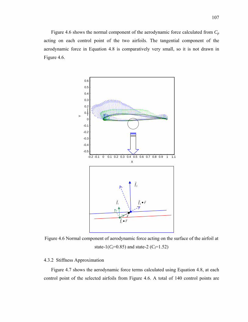
107
Figure 4.6 shows the normal component of the aerodynamic force calculated from Cp
acting on each control point of the two airfoils. The tangential component of the
aerodynamic force in Equation 4.8 is comparatively very small, so it is not drawn in
Figure 4.6.
-0.2 -0.1 0 0.1 0.2 0.3 0.4 0.5 0.6 0.7 0.8 0.9 1 1.1
X
-0.5
-0.4
-0.3
-0.2
-0.1
0
0.1
0.2
0.3
0.4
0.5
0.6Y
Figure 4.6 Normal component of aerodynamic force acting on the surface of the airfoil at
state-1(Cl=0.85) and state-2 (Cl=1.52)
4.3.2 Stiffness Approximation
Figure 4.7 shows the aerodynamic force terms calculated using Equation 4.8, at each
control point of the selected airfoils from Figure 4.6. A total of 140 control points are
1f
2f
rf •1
rf •2
r
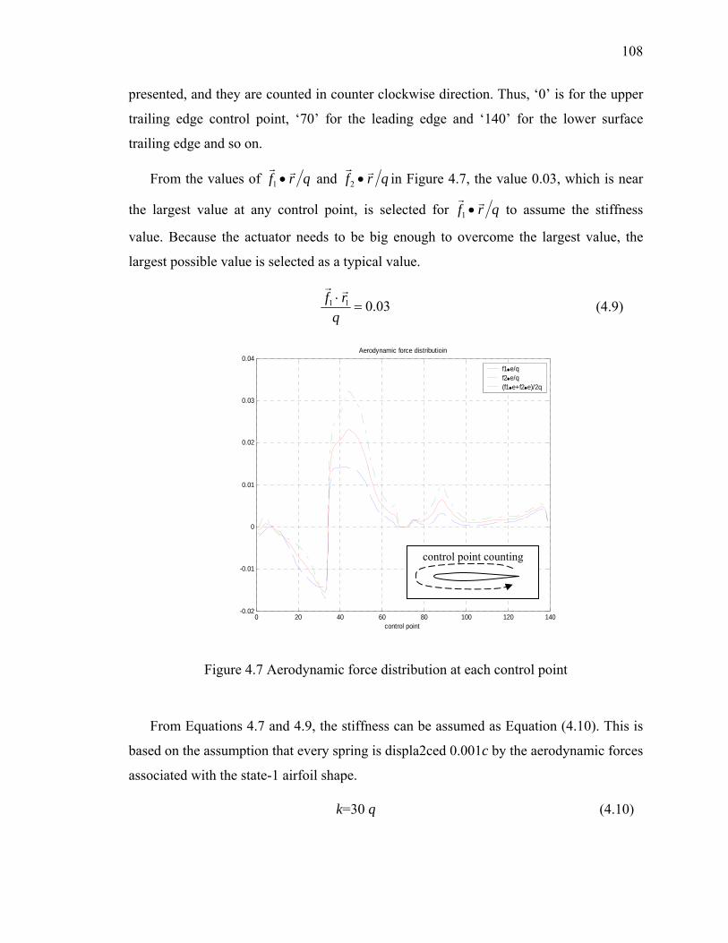
108
presented, and they are counted in counter clockwise direction. Thus, ‘0’ is for the upper
trailing edge control point, ‘70’ for the leading edge and ‘140’ for the lower surface
trailing edge and so on.
From the values of qrf •1 and qrf •2 in Figure 4.7, the value 0.03, which is near
the largest value at any control point, is selected for qrf •1 to assume the stiffness
value. Because the actuator needs to be big enough to overcome the largest value, the
largest possible value is selected as a typical value.
03.011 =⋅q
rf (4.9)
0 20 40 60 80 100 120 140-0.02
-0.01
0
0.01
0.02
0.03
0.04
control point
Aerodynamic force distributioin
f1•e/qf2•e/q(f1•e+f2•e)/2q
Figure 4.7 Aerodynamic force distribution at each control point
From Equations 4.7 and 4.9, the stiffness can be assumed as Equation (4.10). This is
based on the assumption that every spring is displa2ced 0.001c by the aerodynamic forces
associated with the state-1 airfoil shape.
k=30 q (4.10)
control point counting
109
Then, the substitution of Equation (4.10) into Equation (4.6) results in the following
⎥⎥⎦
⎤
⎢⎢⎣
⎡⎟⎟⎠
⎞⎜⎜⎝
⎛Δ
⋅+⋅−Δ= L
qrfrfLqW actuator
)(302
212)(12 (4.11)
This is the work the actuator must do to move the airfoil control point from shape 1 to
shape 2. If this is negative, this indicates the airloads could move the airfoil shape. In the
sensorcraft problem, where the speed and altitude are same for both design conditions,
Equation (4.11) can be rearranged as follows:
[ ]LqrfqrfLConstW actuator Δ⋅+⋅−Δ= )//(30. 212
)(12
Where,
])*()*[(/ 11111 11tdsCndsCqf fp +=
])*()*[(/ 22222 22tdsCndsCqf fp +=
(4.12)
Because the value of q is not changed by the geometry variation, but by the flight
condition, q can be considered as constant value in Equation 4.12. For the total actuator
work needed to morph the airfoil shape, Equation 4.12 is used for each spring modeled in
the airfoil, and these terms are added together.
4.4 Results and Comparison
4.4.1 Effect of Aerodynamic Work Term
The updated actuator work expression, Equation (4.12), is applied to the sensorcraft
problem. Objectives are to minimize the actuation energy and the drag at both flight
conditions when the design lift changes from high to low. For the sensorcraft problem,
the weight of the aircraft reduces as it consumes fuel. Thus, to maintain the same altitude,
the lift should be reduced. Three airfoils are designed for three different flight conditions
as shown in Table 3.1. The objective functions are shown in Equation (4.13). For
110
simplicity, U13 in Equation (2.7) is not included in this test. The airfoil will not change
from 1 to 3 because the lift coefficient is always decreasing.
Minimize: ⎪⎭
⎪⎬⎫
⎪⎩
⎪⎨⎧
++=
)31
31
31(100
),(
321
2312
ddd CCC
UUMaxf
Subject to: 52.11
=lC , ≤1ε solver tolerance
18.12
=lC , ≤2ε solver tolerance
85.03
=lC , ≤3ε solver tolerance
(4.13)
To investigate the effect of the aerodynamic work term in the actuation energy
formulation, two different N-branch GA runs are performed using two sets of different
actuation energy formulations shown in Table 4.1.
Table 4.1 Actuation energy formulation
Aerodynamic load included case Strain energy only case
⎥⎦
⎤⎢⎣
⎡Δ⋅+⋅−Δ= ∑
=
n
iii iiii
LqrfqrfLU1
12212
1212 ))//(30(100
⎥⎦
⎤⎢⎣
⎡Δ⋅+⋅−Δ= ∑
=
n
iii iiii
LqrfqrfLU1
23322
2323 ))//(30(100
⎥⎦
⎤⎢⎣
⎡Δ= ∑
=
n
ii
LU1
21212 )30(100
⎥⎦
⎤⎢⎣
⎡Δ= ∑
=
n
ii
LU1
22323 )30(100
1000 generations (which is considered to be converged), are calculated for each N-
branch GA run. Figure 4.8 compares the Pareto-set of aerodynamic load included versus
strain energy only case. Figure 4.8 shows that the objective values are not very different
for the two sets of results. One of the possible reasons is that it is very difficult to find
airfoils that satisfy the high design lift constraint with a low drag coefficient. The Pareto-
set shows that the aerodynamic force is acting adversely in most of the region. For this
sensorcraft example, the total actuation energy is larger than the strain energy alone for
designs with drag objectives below about 0.83. The reason why the very low energy
solutions appear to gain assistance from the aerodynamic load at the expense of drag
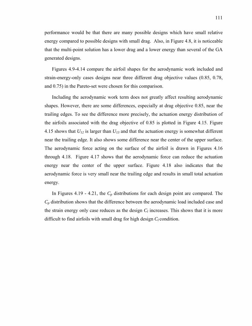
111
performance would be that there are many possible designs which have small relative
energy compared to possible designs with small drag. Also, in Figure 4.8, it is noticeable
that the multi-point solution has a lower drag and a lower energy than several of the GA
generated designs.
Figures 4.9-4.14 compare the airfoil shapes for the aerodynamic work included and
strain-energy-only cases designs near three different drag objective values (0.85, 0.78,
and 0.75) in the Pareto-set were chosen for this comparison.
Including the aerodynamic work term does not greatly affect resulting aerodynamic
shapes. However, there are some differences, especially at drag objective 0.85, near the
trailing edges. To see the difference more precisely, the actuation energy distribution of
the airfoils associated with the drag objective of 0.85 is plotted in Figure 4.15. Figure
4.15 shows that U12 is larger than U13 and that the actuation energy is somewhat different
near the trailing edge. It also shows some difference near the center of the upper surface.
The aerodynamic force acting on the surface of the airfoil is drawn in Figures 4.16
through 4.18. Figure 4.17 shows that the aerodynamic force can reduce the actuation
energy near the center of the upper surface. Figure 4.18 also indicates that the
aerodynamic force is very small near the trailing edge and results in small total actuation
energy.
In Figures 4.19 - 4.21, the Cp distributions for each design point are compared. The
Cp distribution shows that the difference between the aerodynamic load included case and
the strain energy only case reduces as the design Cl increases. This shows that it is more
difficult to find airfoils with small drag for high design Cl condition.
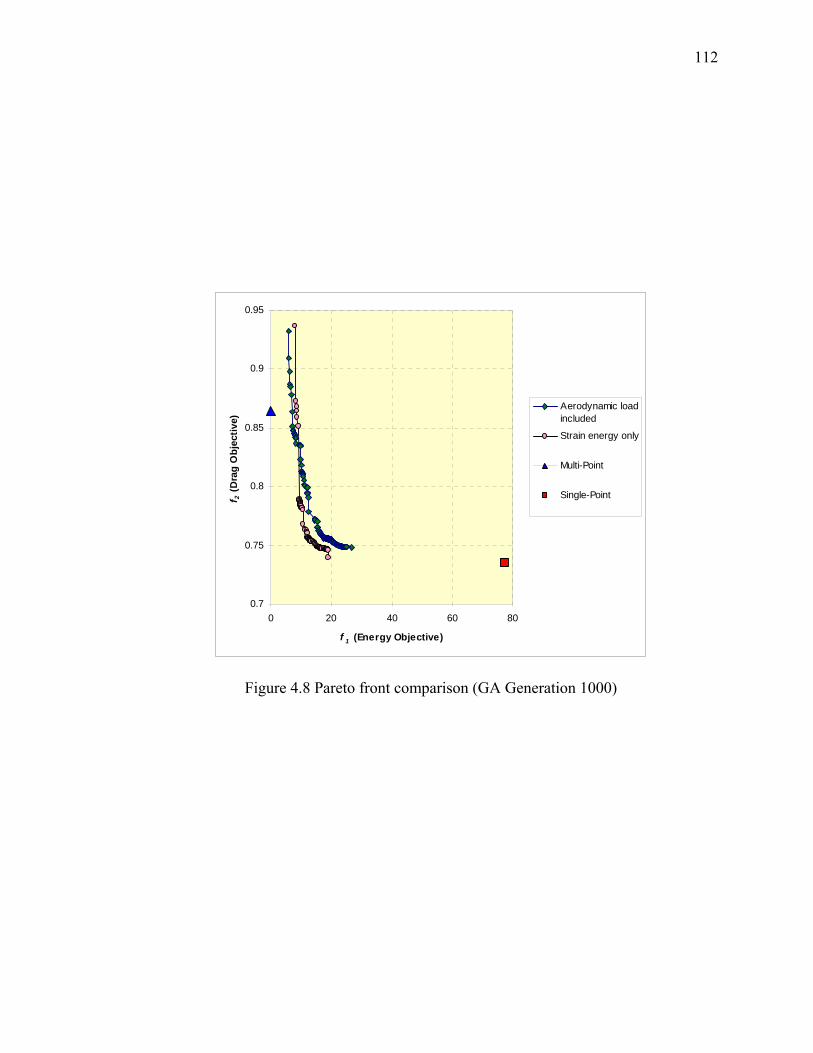
112
0.7
0.75
0.8
0.85
0.9
0.95
0 20 40 60 80
f 1 (Energy Objective)
f 2 (D
rag
Obj
ectiv
e)
Aerodynamic loadincluded
Strain energy only
Multi-Point
Single-Point
Figure 4.8 Pareto front comparison (GA Generation 1000)
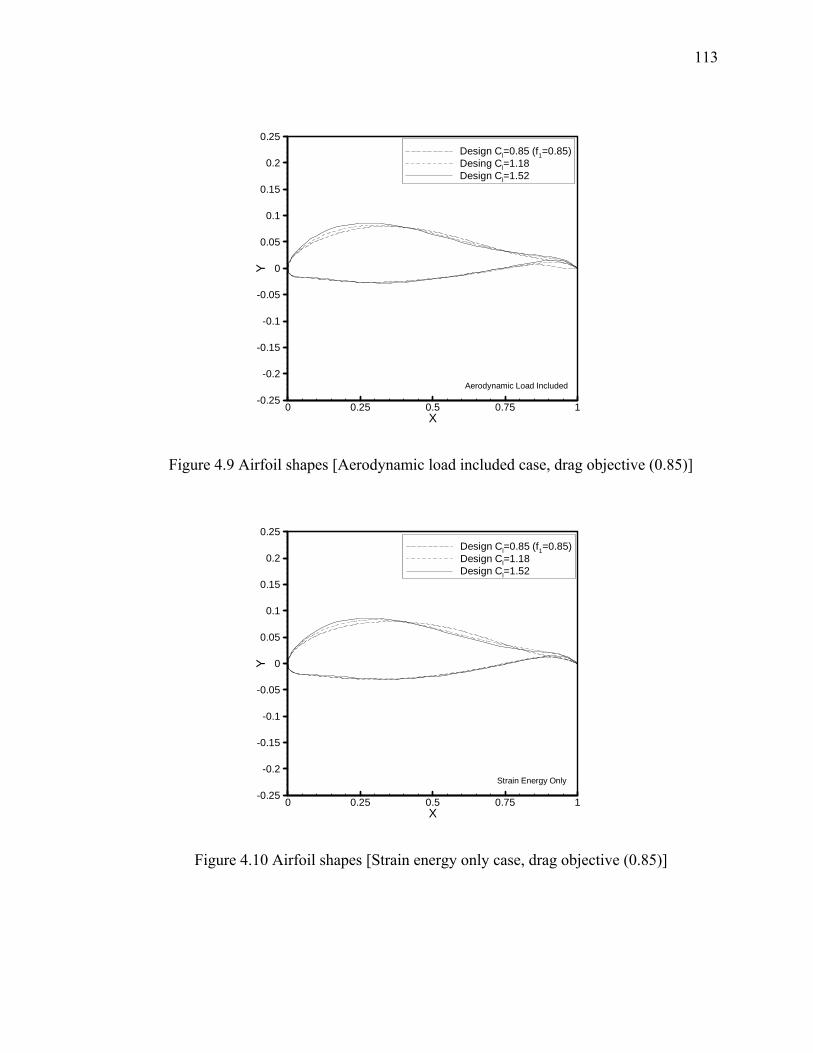
113
0 0.25 0.5 0.75 1X
-0.25
-0.2
-0.15
-0.1
-0.05
0
0.05
0.1
0.15
0.2
0.25
Y
Design Cl=0.85 (f1=0.85)Desing Cl=1.18Design Cl=1.52
Aerodynamic Load Included
Figure 4.9 Airfoil shapes [Aerodynamic load included case, drag objective (0.85)]
0 0.25 0.5 0.75 1X
-0.25
-0.2
-0.15
-0.1
-0.05
0
0.05
0.1
0.15
0.2
0.25
Y
Design Cl=0.85 (f1=0.85)Design Cl=1.18Design Cl=1.52
Strain Energy Only
Figure 4.10 Airfoil shapes [Strain energy only case, drag objective (0.85)]

114
0 0.25 0.5 0.75 1X
-0.25
-0.2
-0.15
-0.1
-0.05
0
0.05
0.1
0.15
0.2
0.25
Y
Design Cl=0.85 (F1=0.78)Design Cl=1.18Design Cl=1.52
Aerodynamic Load Included
Figure 4.11 Airfoil shapes [Aerodynamic load included case, drag objective (0.78)]
0 0.25 0.5 0.75 1X
-0.25
-0.2
-0.15
-0.1
-0.05
0
0.05
0.1
0.15
0.2
0.25
Y
Design Cl=0.85 (f1=0.78)Design Cl=1.18Design Cl=1.52
Strain Energy Only
Figure 4.12 Airfoil shapes [Strain energy only case, drag objective (0.78)]
115
0 0.25 0.5 0.75 1X
-0.25
-0.2
-0.15
-0.1
-0.05
0
0.05
0.1
0.15
0.2
0.25
Y
Design Cl=0.85 (f1=0.75)Design Cl=1.18Design Cl=1.52
Aerodynamic Load Included
Figure 4.13 Airfoil shapes [Aerodynamic load included case, drag objective (0.75)]
0 0.25 0.5 0.75 1X
-0.25
-0.2
-0.15
-0.1
-0.05
0
0.05
0.1
0.15
0.2
0.25
Y
Design Cl=0.85 (f1=0.75)Design Cl=1.18Design Cl=1.52
Strain Energy Only
Figure 4.14 Airfoil shapes [Strain energy only case, drag objective (0.75)]
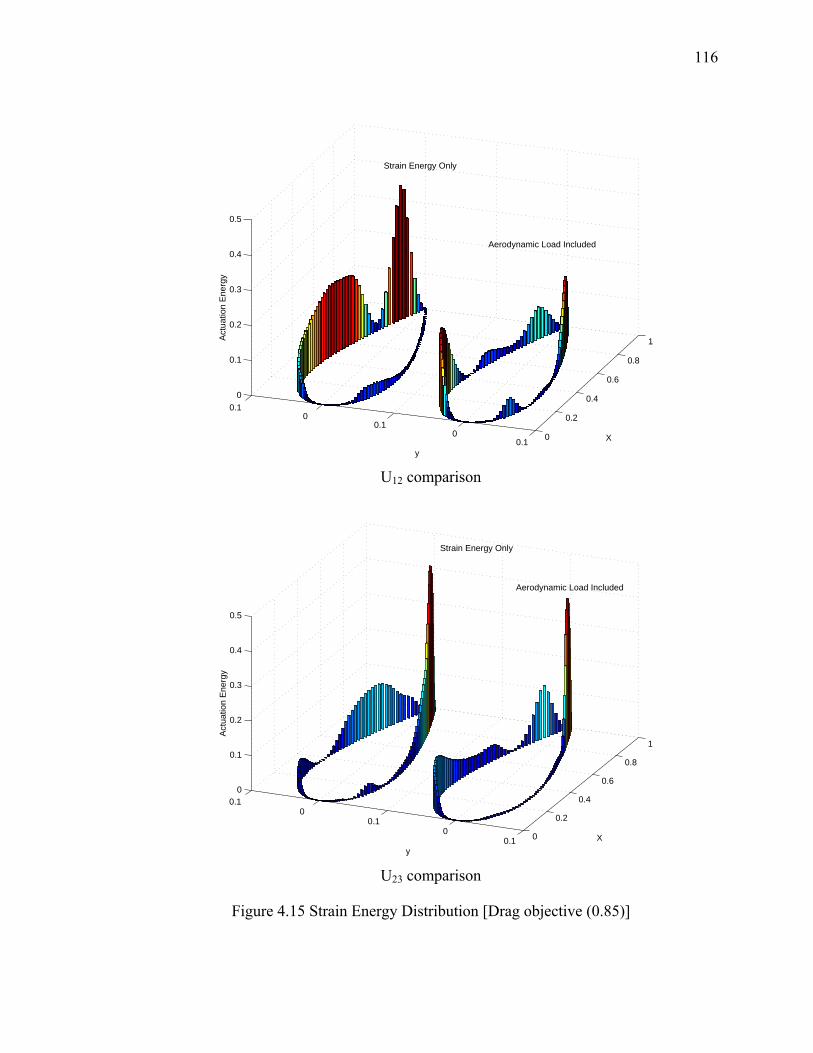
116
0
0.2
0.4
0.6
0.8
1
0.10
0.10
0.1 0
0.1
0.2
0.3
0.4
0.5
X
y
Act
uatio
n E
nerg
y
Strain Energy Only
Aerodynamic Load Included
U12 comparison
0
0.2
0.4
0.6
0.8
1
0.10
0.10
0.1 0
0.1
0.2
0.3
0.4
0.5
X
y
Act
uatio
n E
nerg
y
Strain Energy Only
Aerodynamic Load Included
U23 comparison
Figure 4.15 Strain Energy Distribution [Drag objective (0.85)]
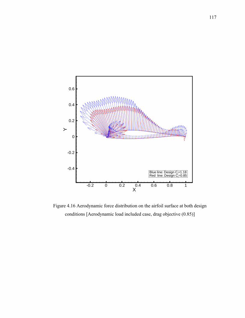
117
-0.2 0 0.2 0.4 0.6 0.8 1X
-0.4
-0.2
0
0.2
0.4
0.6
Y
Blue line: Design Cl=1.18Red line: Design Cl=0.85
Figure 4.16 Aerodynamic force distribution on the airfoil surface at both design
conditions [Aerodynamic load included case, drag objective (0.85)]
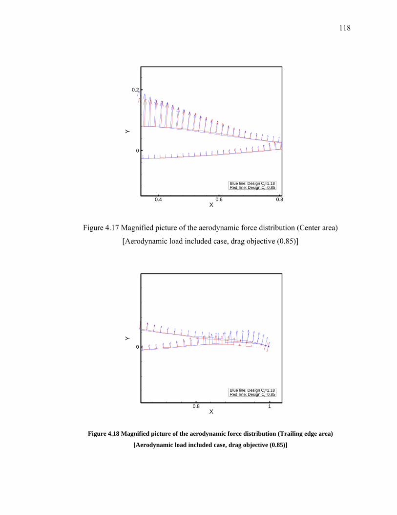
118
0.4 0.6 0.8X
0
0.2
Y
Blue line: Design Cl=1.18Red line: Design Cl=0.85
Figure 4.17 Magnified picture of the aerodynamic force distribution (Center area)
[Aerodynamic load included case, drag objective (0.85)]
0.8 1X
0
Y
Blue line: Design Cl=1.18Red line: Design Cl=0.85
Figure 4.18 Magnified picture of the aerodynamic force distribution (Trailing edge area)
[Aerodynamic load included case, drag objective (0.85)]
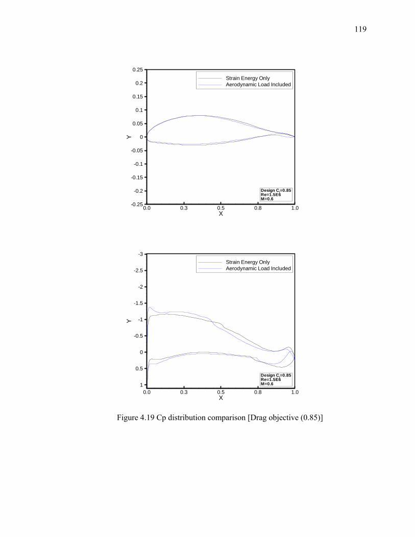
119
0.0 0.3 0.5 0.8 1.0X
-0.25
-0.2
-0.15
-0.1
-0.05
0
0.05
0.1
0.15
0.2
0.25
Y
Strain Energy OnlyAerodynamic Load Included
Design Cl=0.85Re=1.5E6M=0.6
0.0 0.3 0.5 0.8 1.0X
-3
-2.5
-2
-1.5
-1
-0.5
0
0.5
1
Y
Strain Energy OnlyAerodynamic Load Included
Design Cl=0.85Re=1.5E6M=0.6
Figure 4.19 Cp distribution comparison [Drag objective (0.85)]
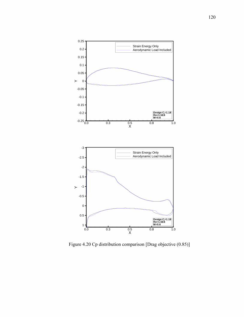
120
0.0 0.3 0.5 0.8 1.0X
-0.25
-0.2
-0.15
-0.1
-0.05
0
0.05
0.1
0.15
0.2
0.25
Y
Strain Energy OnlyAerodynamic Load Included
Design Cl=1.18Re=1.5E6M=0.6
0.0 0.3 0.5 0.8 1.0X
-3
-2.5
-2
-1.5
-1
-0.5
0
0.5
1
Y
Strain Energy OnlyAerodynamic Load Included
Design Cl=1.18Re=1.5E6M=0.6
Figure 4.20 Cp distribution comparison [Drag objective (0.85)]
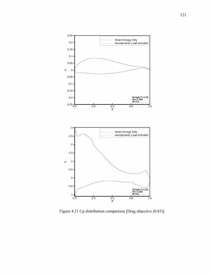
121
0.0 0.3 0.5 0.8 1.0X
-0.25
-0.2
-0.15
-0.1
-0.05
0
0.05
0.1
0.15
0.2
0.25
Y
Strain Energy OnlyAerodynamic Load Included
Design Cl=1.52Re=1.5E6M=0.6
0.0 0.3 0.5 0.8 1.0X
-3
-2.5
-2
-1.5
-1
-0.5
0
0.5
1
Y
Strain Energy OnlyAerodynamic Load Included
Design Cl=1.52Re=1.5E6M=0.6
Figure 4.21 Cp distribution comparison [Drag objective (0.85)]
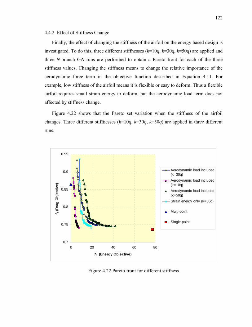
122
4.4.2 Effect of Stiffness Change
Finally, the effect of changing the stiffness of the airfoil on the energy based design is
investigated. To do this, three different stiffnesses (k=10q, k=30q, k=50q) are applied and
three N-branch GA runs are performed to obtain a Pareto front for each of the three
stiffness values. Changing the stiffness means to change the relative importance of the
aerodynamic force term in the objective function described in Equation 4.11. For
example, low stiffness of the airfoil means it is flexible or easy to deform. Thus a flexible
airfoil requires small strain energy to deform, but the aerodynamic load term does not
affected by stiffness change.
Figure 4.22 shows that the Pareto set variation when the stiffness of the airfoil
changes. Three different stiffnesses (k=10q, k=30q, k=50q) are applied in three different
runs.
0.7
0.75
0.8
0.85
0.9
0.95
0 20 40 60 80
f 1 (Energy Objective)
f 2 (D
rag
Obj
ectiv
e)
Aerodynamic load included(k=30q)Aerodynamic load included(k=10q)Aerodynamic load included(k=50q)Strain energy only (k=30q)
Multi-point
Single-point
Figure 4.22 Pareto front for different stiffness
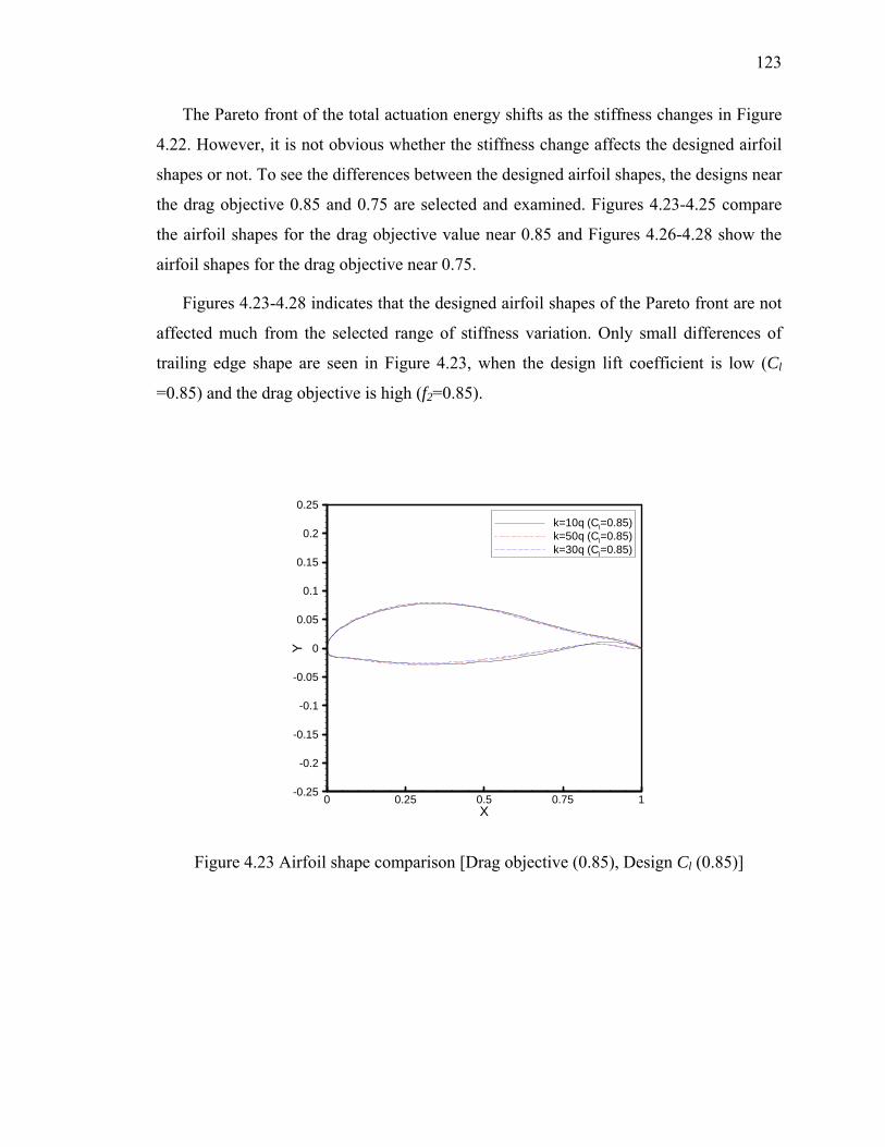
123
The Pareto front of the total actuation energy shifts as the stiffness changes in Figure
4.22. However, it is not obvious whether the stiffness change affects the designed airfoil
shapes or not. To see the differences between the designed airfoil shapes, the designs near
the drag objective 0.85 and 0.75 are selected and examined. Figures 4.23-4.25 compare
the airfoil shapes for the drag objective value near 0.85 and Figures 4.26-4.28 show the
airfoil shapes for the drag objective near 0.75.
Figures 4.23-4.28 indicates that the designed airfoil shapes of the Pareto front are not
affected much from the selected range of stiffness variation. Only small differences of
trailing edge shape are seen in Figure 4.23, when the design lift coefficient is low (Cl
=0.85) and the drag objective is high (f2=0.85).
0 0.25 0.5 0.75 1X
-0.25
-0.2
-0.15
-0.1
-0.05
0
0.05
0.1
0.15
0.2
0.25
Y
k=10q (Cl=0.85)k=50q (Cl=0.85)k=30q (Cl=0.85)
Figure 4.23 Airfoil shape comparison [Drag objective (0.85), Design Cl (0.85)]
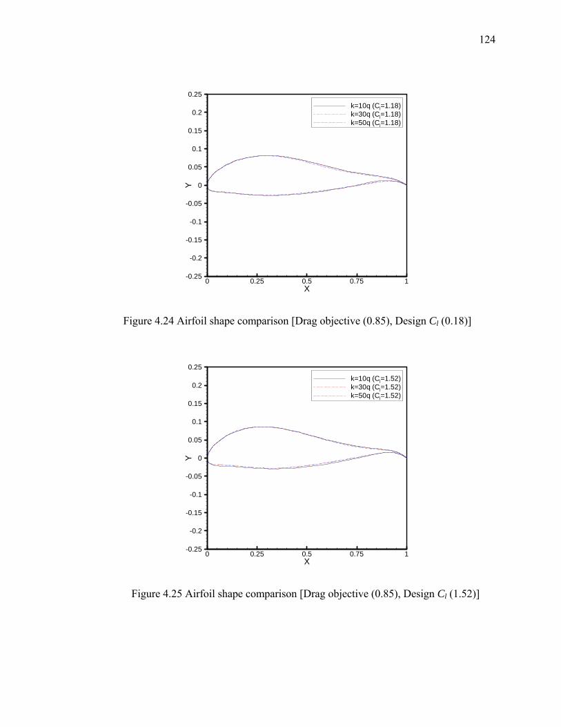
124
0 0.25 0.5 0.75 1X
-0.25
-0.2
-0.15
-0.1
-0.05
0
0.05
0.1
0.15
0.2
0.25
Y
k=10q (Cl=1.18)k=30q (Cl=1.18)k=50q (Cl=1.18)
Figure 4.24 Airfoil shape comparison [Drag objective (0.85), Design Cl (0.18)]
0 0.25 0.5 0.75 1X
-0.25
-0.2
-0.15
-0.1
-0.05
0
0.05
0.1
0.15
0.2
0.25
Y
k=10q (Cl=1.52)k=30q (Cl=1.52)k=50q (Cl=1.52)
Figure 4.25 Airfoil shape comparison [Drag objective (0.85), Design Cl (1.52)]
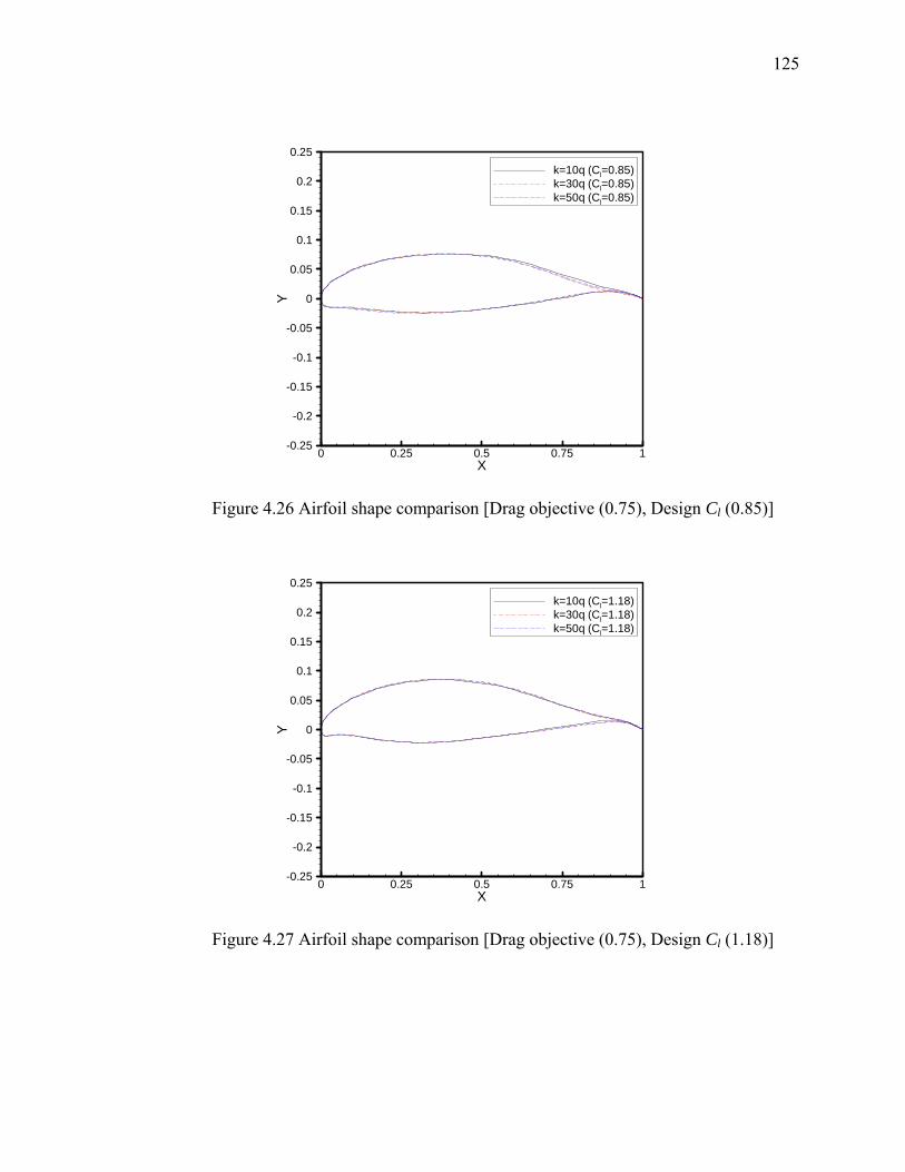
125
0 0.25 0.5 0.75 1X
-0.25
-0.2
-0.15
-0.1
-0.05
0
0.05
0.1
0.15
0.2
0.25
Y
k=10q (Cl=0.85)k=30q (Cl=0.85)k=50q (Cl=0.85)
Figure 4.26 Airfoil shape comparison [Drag objective (0.75), Design Cl (0.85)]
0 0.25 0.5 0.75 1X
-0.25
-0.2
-0.15
-0.1
-0.05
0
0.05
0.1
0.15
0.2
0.25
Y
k=10q (Cl=1.18)k=30q (Cl=1.18)k=50q (Cl=1.18)
Figure 4.27 Airfoil shape comparison [Drag objective (0.75), Design Cl (1.18)]
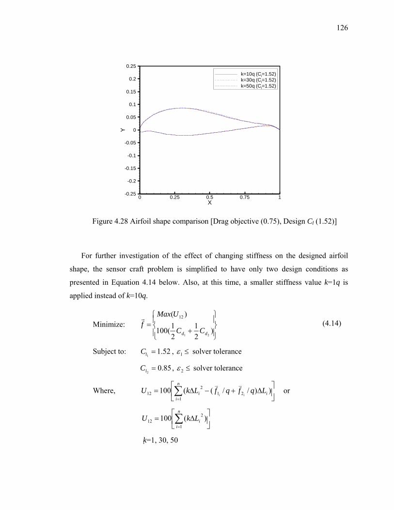
126
0 0.25 0.5 0.75 1X
-0.25
-0.2
-0.15
-0.1
-0.05
0
0.05
0.1
0.15
0.2
0.25
Y
k=10q (Cl=1.52)k=30q (Cl=1.52)k=50q (Cl=1.52)
Figure 4.28 Airfoil shape comparison [Drag objective (0.75), Design Cl (1.52)]
For further investigation of the effect of changing stiffness on the designed airfoil
shape, the sensor craft problem is simplified to have only two design conditions as
presented in Equation 4.14 below. Also, at this time, a smaller stiffness value k=1q is
applied instead of k=10q.
Minimize: ⎪⎭
⎪⎬⎫
⎪⎩
⎪⎨⎧
+=
)21
21(100
)(
21
12
dd CC
UMaxf
Subject to: 52.11
=lC , ≤1ε solver tolerance
85.02
=lC , ≤2ε solver tolerance
Where, ⎥⎦
⎤⎢⎣
⎡Δ+−Δ= ∑
=
n
iii LqfqfLkU
ii1
212
12 ))//((100 or
⎥⎦
⎤⎢⎣
⎡Δ= ∑
=
n
iiLkU
1
212 )(100
k=1, 30, 50
(4.14)
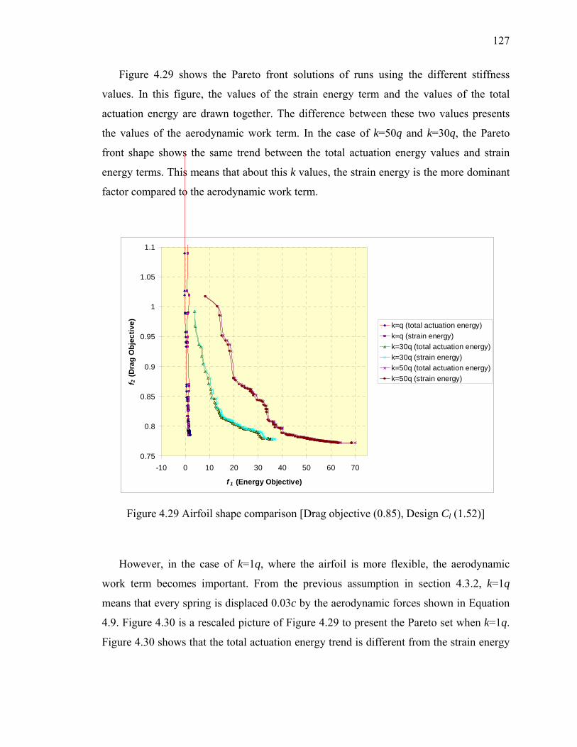
127
Figure 4.29 shows the Pareto front solutions of runs using the different stiffness
values. In this figure, the values of the strain energy term and the values of the total
actuation energy are drawn together. The difference between these two values presents
the values of the aerodynamic work term. In the case of k=50q and k=30q, the Pareto
front shape shows the same trend between the total actuation energy values and strain
energy terms. This means that about this k values, the strain energy is the more dominant
factor compared to the aerodynamic work term.
0.75
0.8
0.85
0.9
0.95
1
1.05
1.1
-10 0 10 20 30 40 50 60 70
f 1 (Energy Objective)
f 2 (D
rag
Obj
ectiv
e) k=q (total actuation energy)k=q (strain energy)k=30q (total actuation energy)k=30q (strain energy)k=50q (total actuation energy)k=50q (strain energy)
Figure 4.29 Airfoil shape comparison [Drag objective (0.85), Design Cl (1.52)]
However, in the case of k=1q, where the airfoil is more flexible, the aerodynamic
work term becomes important. From the previous assumption in section 4.3.2, k=1q
means that every spring is displaced 0.03c by the aerodynamic forces shown in Equation
4.9. Figure 4.30 is a rescaled picture of Figure 4.29 to present the Pareto set when k=1q.
Figure 4.30 shows that the total actuation energy trend is different from the strain energy
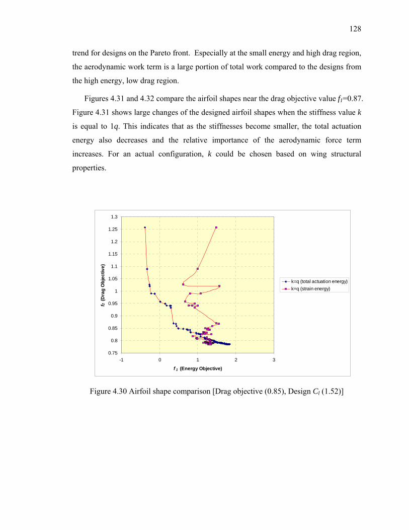
128
trend for designs on the Pareto front. Especially at the small energy and high drag region,
the aerodynamic work term is a large portion of total work compared to the designs from
the high energy, low drag region.
Figures 4.31 and 4.32 compare the airfoil shapes near the drag objective value f1=0.87.
Figure 4.31 shows large changes of the designed airfoil shapes when the stiffness value k
is equal to 1q. This indicates that as the stiffnesses become smaller, the total actuation
energy also decreases and the relative importance of the aerodynamic force term
increases. For an actual configuration, k could be chosen based on wing structural
properties.
0.75
0.8
0.85
0.9
0.95
1
1.05
1.1
1.15
1.2
1.25
1.3
-1 0 1 2 3
f 1 (Energy Objective)
f 2 (D
rag
Obj
ectiv
e)
k=q (total actuation energy)k=q (strain energy)
Figure 4.30 Airfoil shape comparison [Drag objective (0.85), Design Cl (1.52)]
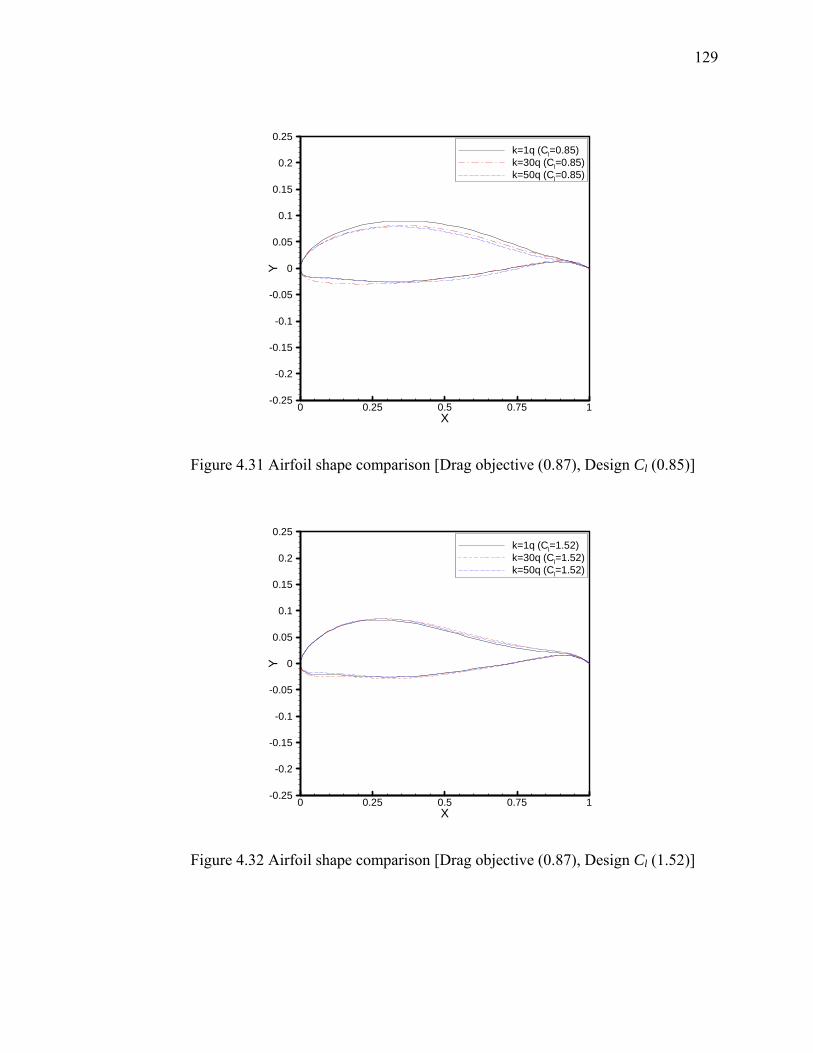
129
0 0.25 0.5 0.75 1X
-0.25
-0.2
-0.15
-0.1
-0.05
0
0.05
0.1
0.15
0.2
0.25
Y
k=1q (Cl=0.85)k=30q (Cl=0.85)k=50q (Cl=0.85)
Figure 4.31 Airfoil shape comparison [Drag objective (0.87), Design Cl (0.85)]
0 0.25 0.5 0.75 1X
-0.25
-0.2
-0.15
-0.1
-0.05
0
0.05
0.1
0.15
0.2
0.25
Y
k=1q (Cl=1.52)k=30q (Cl=1.52)k=50q (Cl=1.52)
Figure 4.32 Airfoil shape comparison [Drag objective (0.87), Design Cl (1.52)]
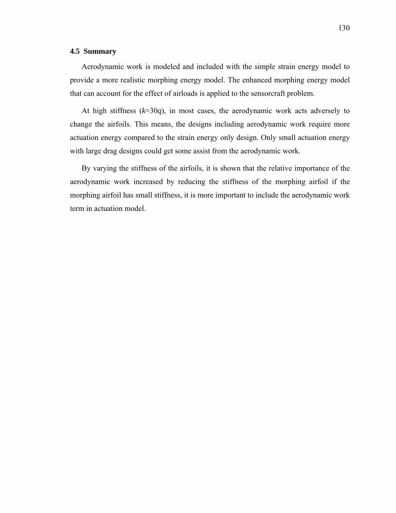
130
4.5 Summary
Aerodynamic work is modeled and included with the simple strain energy model to
provide a more realistic morphing energy model. The enhanced morphing energy model
that can account for the effect of airloads is applied to the sensorcraft problem.
At high stiffness (k=30q), in most cases, the aerodynamic work acts adversely to
change the airfoils. This means, the designs including aerodynamic work require more
actuation energy compared to the strain energy only design. Only small actuation energy
with large drag designs could get some assist from the aerodynamic work.
By varying the stiffness of the airfoils, it is shown that the relative importance of the
aerodynamic work increased by reducing the stiffness of the morphing airfoil if the
morphing airfoil has small stiffness, it is more important to include the aerodynamic work
term in actuation model.
131
CHAPTER 5 CONCLUSIONS
During the research, a parallel genetic algorithm based airfoil optimization strategy
using shape functions is developed. Transonic airfoil design issues are investigated by
comparing the GA(Genetic Algorithm) and a GM (Gradient based Method); this work
employs a Navier-Stokes solver for the transonic drag prediction. Through the research of
transonic airfoil design, it is shown that the GA is more robust in searching global
optimal solution than the GM and the GA combined with the Navier-Stokes code is
affordable for an airfoil design with the help of parallel computing.
There has been great interest in developing technologies that may enable a morphing
aircraft. Such an aircraft can change shape in flight, which would make it possible to
adjust the wing to the best possible shape for any flight condition encountered by the
aircraft. However, there is an actuation energy/cost associated with making these shape
changes. The concept of a morphing aircraft presents a tradeoff between the aerodynamic
performance and the energy or effort needed to morph the aircraft. The development of
optimization strategies incorporating morphing cost is essential during the morphing
aircraft design process to increase the benefits of using morphing technology.
Several multi-objective optimization strategies to design an airfoil set for morphing
aircraft are applied to a low-speed, incompressible flow problem and to a problem
involving low-speed and transonic flow. In the efforts, the relative strain energy needed
to change from on airfoil shape to another is presented as a design objective along with
the drag objective. From this multi-objective optimization strategies, it is identified the
best tradeoff designs of low actuation energy and low drag that lie between the multi-
point shape and the set of single-point shapes. Through these optimization processes,
132
engineers can approach a solution that maximizes the benefits of the morphing
technology, while minimizing the actuation cost.
A simple strain energy model to present morphing cost has been used in previous
work. A new aerodynamic work term is formulated and included into the actuation
energy model in this research. Including the aerodynamic work in morphing airfoil
optimization represents, using pressure on the airfoil to assist a morphing shape change.
In the case of the sensorcraft application, some airfoil sets with small strain energy could
get some assistance from the aerodynamic work. However, for most of the airfoil sets
satisfying the constraints, the aerodynamic force increases the total actuation energy. This
research also demonstrated that it is very important to include aerodynamic work term for
actuation energy calculation when the morphing aircraft wing structure is very flexible.
5.1 Future Directions
In Chapter 3, a simple spring model has been adapted to represent the morphing cost.
The spring model is adequate to show the concept and explain the energy-based design
strategy for morphing aircraft. The strain energy, formulated in the simple spring model,
depends only on the amount of deformation of the airfoil. In reality, the stiffness
distribution of the airfoil or wing will be different depending on the design of the
structure. If a detailed actuation method and structure design is provided, more realistic
actuation energy can be calculated and will generate more accurate designs. However, the
design strategy presented in this thesis can still work for these detailed designs.
Finally, the morphing airfoil problem can be extended to the supersonic flow regime.
This extension will require a dramatic change of the airfoil shape and the morphing cost
will be increased correspondingly. Because the larger change in shape might provide a
broader tradeoff between aerodynamic and actuation energy, the morphing airfoil
optimization strategy suggested in this thesis might contribute more to the supersonic
morphing airfoil design.
133
5.2 Contributions
A system-level design optimization strategy for a morphing airfoil incorporating
minimization of the morphing actuation energy and maximization of the aerodynamic
performance was previously not available. Most of the previous works related to a
morphing aircraft were focused on the development of a light weight actuator device
development. The design strategy presented in this thesis can provide the right reasons
and necessities for morphing aircraft development. Also, the strategy will provide the
directions and generate target shapes for the detail subsystem development and structure
design.
Also, a new aerodynamic work formulation on the morphing airfoil is demonstrated
in this thesis. This aerodynamic work term can be added to the strain energy term to
compute the total energy required for changing the shape of a morphing airfoil. The
aerodynamic work term provides a more realistic actuation energy model especially for a
flexible morphing aircraft. With this formulation, utilizing aerodynamic work suggests
that it is possible to design a morphing airfoil that exploits the airflow to reduce the input
actuation energy.
134
LIST OF REFERENCES
[1] Malone, J. B. et al., ”Airfoil Design Method Using the Navier-Stokes Equations,” Journal of
Aircraft, Vol.28, No3, 1989, pp.216-224.
[2] Anderson, J. D., The Airplane: A History of Its Technology, AIAA, Virgina, 2002.
[3] I.H.Abbott and A.E.V.Doenhoff, Theory of Wing Sections, Dover, New York, 1959.
[4] Harris, C. D., NASA Supercritical Airfoils, NASA TP 2969, 1990.
[5] Bauer, F., Garabedian, P., and Kron, D., A Theory of Supercritical Wing Sections, With
Computer Programs and Examples, Volume 66 of Lecture Notes in Economics and
Mathematical Systems, M.Beckmann and H.P. Kunzi, eds., Springer-Verlag, 1972.
[6] Sobieczky, H., New Design Concepts for High Speed Air Transport, Springer-Verlag, New
York, 1997.
[7] Barger, R. L., and Brooks, C.W., A Streamline Curvature Method for Design of Supercritical
and Subcritical Airfoils, NASA TN D-7770, 1974.
[8] Tranen, T. L., “A Rapid Computer Aided Transonic Airfoil Design Method,” AIAA Paper
74-501, 1974.
[9] Volpe, G., and Melnik, R. E., “A Method for Designing Closed Airfoils for Arbitrary
Supercritical Speed Distributions,” AIAA Paper 85-5023, 1985.
[10] Hicks, R. M., Murman, E. M., and Vaderplaats, G. N., An Assessment of Airfoil Design by
Numerical Optimization, NASA TM X-3092, 1974.
[11] Vanderplaats, G. N., CONMIN-A FORTRAN Program for constrained Function
Minimization, User’s Manual. NASA TM X-62282
[12] Kennelly, R. A., ”Improved Method for Transonic Airfoil Design-by-Optimization, AIAA
Paper 83-1864, 1983.
135
[13] Jameson, A., ”Aerodynamic Design Via Control Theory,” Inst. For Computer Application in
Science and Engineering, Rept. 88-64, NASA Langly, Hampton, VA., Nov.1988.
[14] Abergel. F., and Temam, R., ”On Some Control Problems in fluid Mechanics,” Theoretical
and Computational Fluid Dynamics, Vol. 1, 1990, pp. 303-325.
[15] Holland, J. H., Adaptation in Natural and Artificial Systems, Univ. of Michigan Press, Ann
Arbor, MI, 1974.
[16] Kirkpatrick C.D. et al.,”Optimisation by simulated annealing,” Science, 220, 1983, pp 671-
680.
[17] Goldberg, D. E., Genetic Algorithms in search optimization and machine learning, Addison-
Wesley, MA, 1989.
[18] Hajela, P., “Genetic Search - An Approach to the Nonconvex Optimization Problem,”
AIAA Journal, Vol. 28, No.7, Jul. 1990, pp. 1205-1210.
[19] Drela, M., “Pros & Cons of airfoil optimization,” Frontiers of Computational Fluid
Dynamics-1998,(D. A. Caughey and M. M. Hafez, eds.), World Scientific Publishers, 1998,
pp.363-381.
[20] Samareh, J. A., A Survey of Shape Parameterization Techniques, NASA CP 209136, 1999.
[21] Salomon, D., Computer Graphic and Geometric Modeling, Springer-Verlag, New York,
1999.
[22] Hicks, R. M., Henne, P. A., “Wing Design by Numerical Optimization,” AIAA Journal of
Aircraft, Vol.15, No.7, 1978, pp 407-412.
[23] Obayashi, S., and Tsukahara, T., “Comparison of Optimization Algorithms for
Aerodynamic Shape Design,” AIAA Journal, Vol.35, No.8., Aug. 1997, pp. 1413-1415.
[24] Holst L. T., and Pulliam H. T., “Aerodynamic Shape Optimization Using Real-Number-
Encoded Genetic Algorithm,” AIAA Paper 2001-2473, 2001.
[25] Quagliarella, D. and Della C. A., ”Genetic Algorithms Applied to the Aerodynamic Design
of Transonic Airfoils,” AIAA Paper 94-1896-CP, 1994.
[26] Oyama, A. “Multidisciplinary Optimization of Transonic Wing Design Based on
Evolutionary Algorithms Coupled with CFD Solver,” ECCOMAS, 2000.
136
[27] Jameson A., “Essential Elements of Computational Algorithms for Aerodynamic Analysis
and Design”, NASA CR 97-206268
[28] Rogallo, R. and Moin, P.,”Numerical Simulation of Turbulent Flows,” Annual Review of
Fluid Mechanics, Vol. 16, 1984, pp. 99-137.
[29] Moin, Parviz and Mahesh, Krishnan, “Direct Numerical Simulation: A Tool in Turbulence
Research,”Annual Reviw of Fluid Mechanics, Vol. 30, 1998, pp.539-578.
[30] Sparlart, P. R., Jou, W. H., Strelets, M., and Allmaras, S. R.,”comments on the Feasibility of
LES for Wings and on a Hybrid RANS/LES Approach,” in Advances in DNS/LES, ed. C.
Liu and Z. Liu, Greyden Press, 1997, pp. 137-149.
[31] McGowan, A.R. et al., ”Recent Results from NASA’s Morphing Project,” SPIE Paper
No.4698-11,9th International Symposium on Smart Structure and Materials, 2002,
SanDiego, California
[32] Weisshaar,T.,”Aeroelastic Tailoring for Energy Efficient Morphing Aircraft-Finding the
Right Stuff,” ICASE Morphing Lecture Series, 2001.
[33] Renken, J. H., “Mission Adaptive Wing Camber Control Systems for Transport Aircraft,”
AIAA Paper 85-5006, 1985.
[34] Kudva, J. N., Martin, C. A., Scherer, L. B., Jardine, A. P., McGowan, A. R., Lake, R. C.,
Sendecky, G. and Sanders, B., “Overview of the DARPA/AFRL/NASA Smart Wing
Program,” Proceedings of SPIE. Vol.3674, pp.230-236.
[35] Pendleton, E., Bessette, D., Kehoe, M., and Perry, B., “A Flight Research Program for
Active Aeroelastic Wing Technology,” AIAA Paper 96-1574, 1996.
[36] Marks, P.,”The next 100 years of flight,” NewScientist.com news service, Dec. 2003.
[37] Obayashi, S., and Tsukahara, T., “Comparison of Optimization Algorithms for
Aerodynamic Shape Design,” AIAA Journal, Vol.35, No.8., Aug. 1997, pp. 1413-1415.
[38] Holst L. T., and Pulliam H. T., “Aerodynamic Shape Optimization Using Real-Number-
Encoded Genetic Algorithm,” AIAA Paper 2001-2473, 2001.
[39] Prock, B. C., Weisshaar T. A., Crossley, W.A., ”Morphing airfoil shape change
optimization with minimum actuator energy as an objective,” 9th AIAA/ISSMO
Symposium on Multidisciplinary Analysis and Optimization, Atlanta, Georgia, 2002.
137
[40] Smareh, J. A., A Survey of Shape Parameterization Techniques, NASA CP 209136, 1999.
[41] Hager, J. O., Eyi, S., Lee, K. D., “Two-point transonic airfoil design using optimization for
improved off-design performace,” AIAA Journal of Aircraft, Vol.31, No5, 1994, pp. 1143-
1147.
[42] Chang, I, et al.. Geometric Analysis of Wing Sections, NASA TM 110346, 1995.
[43] Ramamoorthy, P., and Padmavathi, K., “Airfoil Design by Optimization, Journal of
Aircraft,” Vol. 14, pp. 219-221, 1977.
[44] Salomon, D., Computer Graphic and Geometric Modeling, Springer-Verlag, New York,
1999.
[45] Harris, D., C., NASA Supercritical Airfoils, NASA TP 2969, 1990.
[46] Selig, M., “UIUC Airfoil Data Site,” [http://amber.aae.uiuc.edu/~m-selig/ads.html],
accessed Feb. 2002.
[47] Drela, M., “Pros & Cons of airfoil optimization,” Frontiers of Computational Fluid
Dynamics-1998,(D. A. Caughey and M. M. Hafez, eds.), World Scientific Publishers, 1998,
pp.363-381.
[48] Srinivasan, G. R., Baeder, J. D., ”Flowfield of a Lifting Rotor in Hover: A Navier-Stokes
Simulation,” AIAA Journal, Vol.30, No.10, 1992, pp.2371-2378.
[49] Roe, P. L., “Approximate Riemann solvers, parameter vectors and difference schemes,”
Journal of Computational Physics, 43, 1981, pp. 357-72.
[50] Anderson, W. K., Thomas, J. L., and van Leer, B., “A Comparison of Finite Volume Flux
Vector Splitting for the Euler Equations,” AIAA Paper 85-0122, Jan. 1985.
[51] Jameson, A., and Yoon, S., “Lower-Upper Implicit Schemes with Multiple Grids for the
Euler Equaitons,” AIAA Journal, Vol. 25, No. 7, 1987, pp.929-935.
[52] Yoon,S.,and Jameson, A.,”An LU-SSOR Scheme for the Euler and Navier-Stokes
Equations,” AIAA Paper 87-0600, Jan.1987.
[53] “Experimental Data base for Computer Program Assessment”, AGARD advisory report,
No.138, 1979.
138
[54] Goldberg, D. E., Genetic Algorithms in search optimization and machine learning, Addison-
Wesley, MA, 1989.
[55] Hajela, P., “Genetic Search - An Approach to the Nonconvex Optimization Problem,”
AIAA Journal, Vol. 28, No.7, Jul. 1990, pp. 1205-1210.
[56] Jones, B. R., Crossley, W. A., Lyrintzis, A. S., “Aerodynamic and Aeroacoustic
Optimization of Airfoils via a Parallel Genetic Algorithm,” AIAA Journal of Aircraft, Vol.
37, No. 5, Nov.-Dec. 2000, pp. 1088-1096.
[57] Zoutendijk, G., Methods of Feasible Directions, Elsevier, Amsterdam, 1960.
[58] Williams, E. A., Crossley, W. A., “Empirically-derived population size and mutation rate
guidelines for a genetic algorithm with uniform crossover,” WSC2:2nd Online World
Conference on Soft Computing in Engineering Design and Manufacturing, June 1997.
[59] Zoutendijk, G., Methods of Feasible Directions, Elsevier, Amsterdam, 1960.
[60] Reich, W. G., Bowman, C. J., Sanders, B., “Large-Area Aerodynamic Control for High-
Altitude Long-Endurance Sensor Platforms,” Journal of Aircraft, Vol. 42, No.1, Jan 2005.
[61] Martin, E. T., Hassan, R. A., Crossley, W. A., “Comparison of the N-Tournament Genetic
Algorithm and the Multi-Objective Genetic Algorithm,” AIAA Journal, Vol.42, No.6, June
2004.
[62] Fonseca, C., and Fleming, P., “ Genetic Algorithms for Multiobjective Optimization:
Formulation, Discussion and Generalization,” Proceedings of the Fifth International
Conference on Genetic Algorithms, edited by S. Forrest, Morgan Kaufmann, San Mateo,
CA, 1993, pp.416-423.
[63] Drela, M., ”XFOIL: An Analysis and Design System for Low Reynolds Number Airfoils,”
Conference on Low Reynolds Number Airfoil Aerodynamics, University of Notre Dame,
June 1989.
[64] Crossley, W. A. , Nankani, K., Raymer, D. P., “ Comparison of Bit-String Affinity and
Consecutive Generation Stopping Criteria for Genetic Algorithms,” AIAA Paper 2004-449,
2004.
[65] “Global Hawk First Flight,” Aviation Week & Space Technology, March 9, 1998.
139
VITA
03/1989 - 02/1993 Bachelor of Science
Department of Aeronautical and Mechanical Engineering
Hankuk Aviation University, Seoul, Korea
03/1993 - 02/1995 Master of Science
Department of Aerospace Engineering
Korea Advanced Institute of Science and Technology (KAIST),
Taejon, Korea
03/1995 - 07/2000 Research Engineer
Aircraft Division
Korea Aerospace Research Institute, Taejon, Korea
08/2000 - 12/2005 Doctor of Philosophy
School of Aeronautics and Astronautics
Purdue University, West Lafayette, IN
Top Related