


Languages
Pages
Legal


International Journal of Communication Systems and Network Technologies
Vol.5, No.1, 2016
DOI- 10.18486/ijcsnt.2016.5.1.01 1
ISSN-2053-6283
Adaptive Cognitive System Applied to WSN Decisions at
Nodes with a Fuzzy Logic Approach
Marcel Stefan Wagner
Department of Electronic Systems Engineering, Polytechnic School, University of São Paulo, São Paulo, Brazil
Miguel Arjona Ramírez
Department of Electronic Systems Engineering, Polytechnic School, University of São Paulo, São Paulo, Brazil
Wagner Luiz Zucchi
Department of Electronic Systems Engineering, Polytechnic School, University of São Paulo, São Paulo, Brazil
Abstract -The Adaptive Cognitive System (ACS) presented here is based on the concept of cognition applied to
Wireless Sensor Networks (WSN) concerning aspects related to memory, history and decision making over
network node tasks. The use of cognitive features in the WSN scope allows the nodes to make better decisions
about conflicts or anomalies arising from node or route failures that probably will affect the performance
network as a whole. Moreover, with the use of cognitive aspects in feedback processes to make decisions in a
multilayer approach, it is possible to obtain an improvement in the data transmitted end-to-end by the nodes.
The decision process consists of adjustments in memory, queue, route protocols and energy consumption. A
Fuzzy Inference System (FIS) is proposed for decision making from the vector collected from the network, and
this logic determines the adjustments to be applied to the network. This inference system is expandable,
allowing other rules, metrics and parameters to be added to the analysis for more flexibility and improved
performance.
Keywords – Wireless; WSN; Cognitive Network; Fuzzy Logic.
I. Introduction
Wireless Sensor Networks (WSN) represent a major network
research area since it fosters different kinds of applications
and suits interests that range from a simple exchange of
information to the transmission and reception of significant
data. Safety aspects are not only the important parameters to
be explored in WSN.
Algorithms and protocols focused on the transmission
speed, packet delivery increase and node energy economy
are well surveyed in this field. But features related to
performance and Quality of Service (QoS) are important for
evaluating whether the network meets its goals and for rating
its acceptance.
Focusing on the improvement of network performance, this
work applies a number of cognitive processes within WSN
nodes to introduce intelligence based on memory and critical
analysis which provide the means for the decision making
process, that will be described in the section IV. The
combination of cognition with WSN to solve network
problems underlines the need for studies encompassing
different areas of expertise in search of elaborate alternative
solutions.
Cognitive parameters can be inserted in logical mechanisms
as the system’s intelligent part, allowing it to act on the
collected data obtained from network feedback vectors
according to history and memory aspects, observing yet the
network’s policies and purposes. Once the data are gathered,
the cognitive process is able to proceed to the decision
making stage.
In order to provide the means for node decisions, an analysis
based on a decision-threshold is made with system’s critical
table values collected from the network monitoring vector
parameters, as described in next sections. These vectors are
International Journal of Communication Systems and Network Technologies
Vol.5, No.1, 2016
DOI- 10.18486/ijcsnt.2016.5.1.01 2
ISSN-2053-6283
essential for system analysis because they are the source of
the critical tables. Specifically, these vectors are obtained
from Prowler simulator running over MATLAB platform.
Some researchers in this area treat the theme focusing on
prediction routing schemes, such as Jie Li et al [1], who
suggest a routing algorithm based on a traffic prediction
model known as Efficient Traffic Aware Multi-path Routing
(ETAMR). The ETAMR algorithm uses traffic distribution
and load to build a multi-path routing using a prediction
model. Metrics such as node energy consumption or even
network throughput are not considered in this model and are
the matter of their future works.
In contrast with [1], instead of relying on a prediction
mechanism to change some aspects of network routing, the
present work uses the actual readings of network data,
collected in predetermined intervals, to execute cognitive
processes and provide actuation on network aspects such as
routing. This allows for more coherent alterations, not only
in routing aspects, but in the nodes processing schemes,
buffer operation and energy consumption economy.
The algorithm developed here emphasizes the QoS regarding
end-to-end packet delivery ratio among network nodes in
scenarios with random node’s movement. Therefore, control
over the amount of energy consumption in the nodes will be
approached as part of the cognitive process.
In [10] another prediction model is presented and in [2] and
[11] the importance of WSN integration and application in
Internet of Things (IoT) meaning are considered. [3] and [5]
gives us examples of WSN simulations using NS-2 software.
[6] and [7] treat about cognition applied into WSN
environments. [4], [8] and [9] have examples of certain
difficulties or anomalies concerning sensor networks.
The rest of paper is organized as follows. Section II
describes the node’s internal architecture and interface into
block’s diagrams. Section III represents the environment
description and important features related to nodes
dimension. Section IV corresponds to the system’s
development and organization. Section V describes the
Fuzzy Logic implementation. Section VI shows the results.
Finally, concluding remarks and future survey directions are
given in Section VII.
II. Node Description
It is important to know the node’s internal architecture,
as well as the modules connections of sensor nodes.
Therefore, it can be viewed ahead the internal structure of
the sensor studied in this paper.
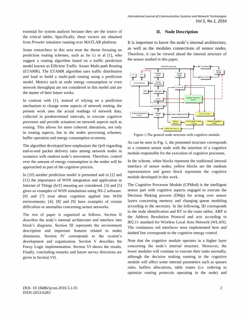
Figure 1.The general node structure with cognitive module.
As can be seen in Fig. 1, the presented structure corresponds
to a common sensor node with the insertion of a cognitive
module responsible for the execution of cognitive processes.
In the scheme, white blocks represent the traditional internal
interface of sensor nodes, yellow blocks are the medium
representation and green block represents the cognitive
module developed in this work.
The Cognitive Processor Module (CPMod) is the intelligent
sensor part with cognitive aspects engaged to execute the
Decision Making process (DMp) for acting over sensor
layers concerning memory and changing queue modeling
according to the necessity. In the following, ID corresponds
to the node identification and RT to the route tables. ARP is
the Address Resolution Protocol and acts according to
802.11 standard for Wireless Local Area Network (WLAN).
The continuous red interfaces were implemented here and
dashed line corresponds to the cognitive energy control.
Note that the cognitive module operates in a higher layer
concerning the node’s internal structure. Moreover, the
lower modules will continue to execute their tasks normally,
although the decision making running in the cognitive
module will affect some internal parameters such as queues
rules, buffers allocations, table routes (i.e. ordering to
optimize routing protocols operating in the node) and
International Journal of Communication Systems and Network Technologies
Vol.5, No.1, 2016
DOI- 10.18486/ijcsnt.2016.5.1.01 3
ISSN-2053-6283
antenna power gain to accomplish network performance
adjustments.
III. Environment and Node Details
This work considers the application of dynamic or
differentiated media. The study comprises networks with
random node movement, so it is not limited to a single
scenario. The network environment is variable, thus any link
between two nodes should be reestablished if any alteration
in the environment occur or due to the changes in nodes
positions, so the system can adapt to it and to its logical
routes configurations.
To identify the node dimensions for the environment
applied, the system-related variable is given by (1):
( ) (1)
From (1), FV represents the node variability number between
[0,1] for a single trajectory and it is composed by the
following: PV, accounting for the node position variation; RV,
accounting for the node radius variation; LV represents the
variation in the number of links established by nodes and NV
is the number of nodes variation in the network.
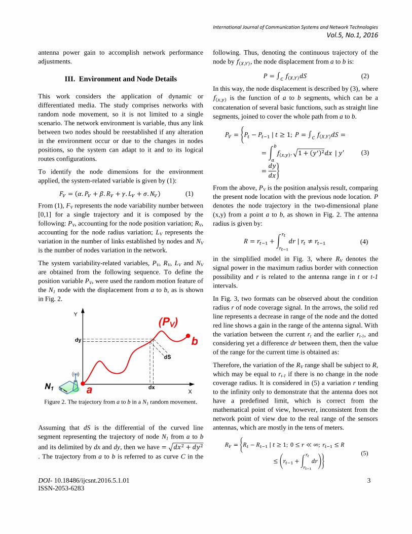
The system variability-related variables, PV, RV, LV and NV
are obtained from the following sequence. To define the
position variable PV, were used the random motion feature of
the N1 node with the displacement from a to b, as is shown
in Fig. 2.
Figure 2. The trajectory from a to b in a N1 random movement.
Assuming that dS is the differential of the curved line
segment representing the trajectory of node N1 from a to b
and its delimited by dx and dy, then we have √
. The trajectory from a to b is referred to as curve C in the
following. Thus, denoting the continuous trajectory of the
node by ( ), the node displacement from a to b is:
( ) (2)
In this way, the node displacement is described by (3), where
( ) is the function of a to b segments, which can be a
concatenation of several basic functions, such as straight line
segments, joined to cover the whole path from a to b.
{ ( )
∫ ( ) √ ( )
}
(3)
From the above, PV is the position analysis result, comparing
the present node location with the previous node location. P
denotes the node trajectory in the two-dimensional plane
(x,y) from a point a to b, as shown in Fig. 2. The antenna
radius is given by:
∫
(4)
in the simplified model in Fig. 3, where RV denotes the
signal power in the maximum radius border with connection
possibility and r is related to the antenna range in t or t-1
intervals.
In Fig. 3, two formats can be observed about the condition
radius r of node coverage signal. In the arrows, the solid red
line represents a decrease in range of the node and the dotted
red line shows a gain in the range of the antenna signal. With
the variation between the current rt and the earlier rt-1, and
considering yet a difference dr between them, then the value
of the range for the current time is obtained as:
Therefore, the variation of the RV range shall be subject to R,
which may be equal to rt-1 if there is no change in the node
coverage radius. It is considered in (5) a variation r tending
to the infinity only to demonstrate that the antenna does not
have a predefined limit, which is correct from the
mathematical point of view, however, inconsistent from the
network point of view due to the real range of the sensors
antennas, which are mostly in the tens of meters.
{
( ∫
)}
(5)

International Journal of Communication Systems and Network Technologies
Vol.5, No.1, 2016
DOI- 10.18486/ijcsnt.2016.5.1.01 4
ISSN-2053-6283
The range of the antenna signal is also directly linked to the
signal fading effect in the transmission medium, which in
wireless communications is Rayleigh, i.e. the greater the
distance between the nodes, the larger is the signal loss
according to the Rayleigh curve ( ) of the Probability
Density Function (PDF), which is directly related to distance
from the source node, and is presented in Fig. 4 and having
the notation R ~ Rayleigh( ), where is the scaling factor
for the signal fading.
Figure 3. Node signal coverage feature in WSN.
Equation (6) represents the PDF of x. As can be seen in Fig.
4, x is the distance and is the fading factor for the curve.
Fig. 4a shows the PDF for a sequence of 5 simulations of
and Fig. 4b shows the distribution function for the same 5
simulations of changes.
Figure 4. PDF and distribution function of Rayleigh for
communication channel.
It is also noted in Fig. 4a that the larger gets the straighter
the curve. Also, in Fig. 4b, as increases, the function
spreads wider.
( )
{
} (6)
Equation (7) shows the distribution function for the
presented Fig. 4b.
( ) {
} (7)
Therefore, considering the fading effect of (6) and applying
( ) from the (7) in the position equation (5), it has:
{ ( ( ))
( ∫
) ( ( ))}
(8)
After that, connections will probably will fail with 70%
chance and current connections will drop with over 85%.
)(1 ;10;1| Sneigneigttv RNNLtLLL (9)
With respect to the LV parameter, L is associated to the
number of links established by nodes. corresponds to
the number of neighboring nodes that should be inside the
radius area of source node.
1|1 tNNN ttv (10)
Equation (10) shows NV as the current number of nodes in
the network. It can be changed according to the insertion or
loss of nodes in the network. The ratios among PV, RV, LV
and NV are the factors α, β, γ and σ respectively, and are
given by:
∑( )
{
|
argmax( )|
|
argmax( )|
|
argmax( )|
|
argmax( )|
(11
)
International Journal of Communication Systems and Network Technologies
Vol.5, No.1, 2016
DOI- 10.18486/ijcsnt.2016.5.1.01 5
ISSN-2053-6283
Equation (11) refers to the proportions related to the
system’s variability factors: α, the position ratio; β, the node
radius ratio; γ, the ratio of the node’s possible connections
and σ, the ratio of number of nodes in the network.
The variables PV, RV, LV and NV are obtained from (2)-(10)
and the relations in the variability detection are presented in
pseudo-code part posted ahead, where t represents current
time and t-1 represents time in the previous step.
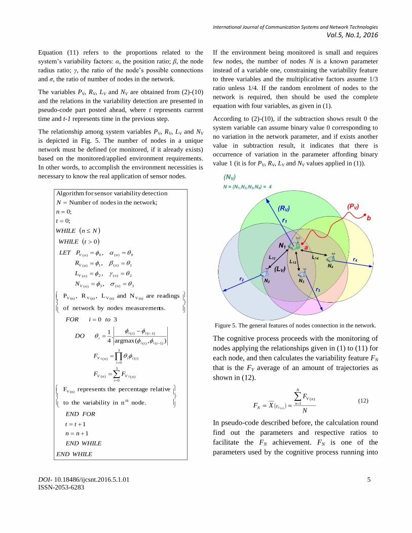
The relationship among system variables PV, RV, LV and NV
is depicted in Fig. 5. The number of nodes in a unique
network must be defined (or monitored, if it already exists)
based on the monitored/applied environment requirements.
In other words, to accomplish the environment necessities is
necessary to know the real application of sensor nodes.
WHILEEND
WHILEEND
nn
tt
FOREND
FF
F
DO
toiFOR
N
L
R
PLET
tWHILE
NnWHILE
t
n
N
iniVnV
i
tiiniV
titi
titi
i
nnV
nnV
nnV
nnV
1
1
node.ninyvariabilittheto
relativepercentagetherepresentsF
),(argmax.
4
1
30
ts.measuremennodesbynetworkof
readingsareNandL,R,P
,
,
,
,
0
;0
;0
network; in the nodes ofNumber
detectioniability sensor varfor Algorithm
th
(n)V
3
0)()(
3
0
)()(
)1()(
)1()(
(n)V(n)V(n)V(n)V
3)(3)(
2)(2)(
1)(1)(
0)(0)(
If the environment being monitored is small and requires
few nodes, the number of nodes N is a known parameter
instead of a variable one, constraining the variability feature
to three variables and the multiplicative factors assume 1/3
ratio unless 1/4. If the random enrolment of nodes to the
network is required, then should be used the complete
equation with four variables, as given in (1).
According to (2)-(10), if the subtraction shows result 0 the
system variable can assume binary value 0 corresponding to
no variation in the network parameter, and if exists another
value in subtraction result, it indicates that there is
occurrence of variation in the parameter affording binary
value 1 (it is for PV, RV, LV and NV values applied in (1)).
Figure 5. The general features of nodes connection in the network.
The cognitive process proceeds with the monitoring of
nodes applying the relationships given in (1) to (11) for
each node, and then calculates the variability feature FN
that is the FV average of an amount of trajectories as
shown in (12).
N
F
XF
N
nnV
FN nV
1
)(
)(
(12)
In pseudo-code described before, the calculation round
find out the parameters and respective ratios to
facilitate the FN achievement. FN is one of the
parameters used by the cognitive process running into

International Journal of Communication Systems and Network Technologies
Vol.5, No.1, 2016
DOI- 10.18486/ijcsnt.2016.5.1.01 6
ISSN-2053-6283
CPMod to provide Decision Making process (DMp)
and it will be described in next section.
IV. System Features and Development
The cognitive process uses the memory vector VM, the
variability feature FN (described in previous section) and the
input signal SI(n) to generate the output signal SO(n) that
controls the system with cognitive process.
In the cognitive process the comparator result is the mean
squared error (MSE) Ԑ between the received signal SI(n) and
the output signal SO(n) and it is used for system adequacy.
For a given input signal SI(n) composed by network
variability feature and memory vector (the memory vector
will be described further, but it comprises data obtained from
the network’s nodes regarding connections successes or
failures in addition to route information), the cognitive
process uses FN, VM and Ԑ to identify possible problems in
the network and to act on the output signal SO(n) with a
control vector VC.
Fig. 6 illustrates the interfaces and connections taking place
in the cognitive process regarding internal development of
initial CPMod (iCPMod).
The signal SI(n) derives from the combination of FN and VM,
while VC acts on SO(n). FN and VM are indicators of system
environment situation. With the analysis of these two
parameters, SI(n) signal can be composed for error
calculation. The results applying these indicators are shown
in the section VI.
Figure 6. Block diagram of the cognitive process interconnection.
A. Memory Vector
The Memory Vector VM is in the core of the adaptive
cognitive module studied here since it allows the cognitive
process to store information regarding network and its
nodes, establishing the history of the network situations and
memory.
This vector results from the compilation of instant data
regarding the monitored environment within time slots after
each 5 seconds is recommended. With VM it is possible to act
on the environment using the DMp to generate DM vectors.
RFSM VVVV ,, (13)
Equation (13) introduces VM matching to the memory vector
composed by: VS as the vector containing the successes of
nodes connections; VF as the vector containing the failures in
the nodes and VR as a vector of valid routes collected from
RT. The components of VS, VF and VR are described briefly
in Table I.
Table I. Memory Vector Components
Vec
tor
Ty
pe Components and Description
Description Components Decision
VS Success
Vector
Successful end-to-
end connection,
End-to-end delay,
Rate of effectively
delivered data.
By the
routes with a
higher
probability
of end-to-
end packet
delivery
success.
VF Failure Vector
Node disconnected
three times in a
row, Unresponsive
node with reply
message (RREP).
Avoiding
these nodes
for a given
period of
time.
VR Route Vector
Valid routes,
Origin node,
Destination node,
Number of hops to
destination.
By the best
route
according to
the valid
routes
history.
The VM application for the DM classification will be
described ahead and this feature is present on the CPMod as
an instance of DM analysis, as in (15).
B. Error Vector
Basically, the error vector Ԑ works with the relative error
MSE of the cognitive module measurements input SI(n) and
output SO(n) signals. SI(n) is composed by the variability

International Journal of Communication Systems and Network Technologies
Vol.5, No.1, 2016
DOI- 10.18486/ijcsnt.2016.5.1.01 7
ISSN-2053-6283
feature and memory vector, and SO(n) works with control
vector (described in D division of this section) and memory
vector.
{ ( ) estimate
( ) real value
( ) ∑( )
(14)
The composition of this feature appears in the third
parameter for DM analysis, as shown in (15).
C. Decision Making Vector
The procedure for Decision Making process (DMp) is
conducted by the cognitive process and it takes into the
account of environment variability feature FN, the memory
vector VM and the error Ԑ, seeking for the optimal network
configuration and the adjustment of the employed routing
protocol.
DM is assigned according to the expected quality of the task
and its action is directly related to the Decision Limit (DL).
The threshold DL corresponds to a probabilistic value for the
adjustment of the system resulting from the combination of
FN, VM and Ԑ according to the range entrance (DM
description) given in Table II.
,, MN VFDM (15)
Five abstraction levels were adopted based on Quality of
Experience (QoE) since they represent the network
conditions and allow VC actuation. DL is calculated using the
inverse of the average of DM composition as described in
(16).
For the measurement level regarding the network situation,
as mentioned before, DL is calculated based on the inverse
of DM average, according to (16). The graphical relationship
for DL is depicted in Fig. 7.
%100,1
(%)1001
,1
,,
(%),,
,,(%),,
1,,
DLX
XDLX
N
VF
X
MN
MN
MN
iii
MN
VF
VF
VF
N
i
MN
VF
(16)
The smaller DL, in percentage, the better is the network
condition and, similarly, the greater DL the worst is the
network situation, therefore more significant actions should
be taken by the CPMod. Furthermore, in order to keep the
network with controlled or regular situation, DL level must
be under 49.9% range.
Figure 7. Example of relationship between DL and DM.
Table I. Decision Making According To the Dl Threshold
DM
Descripti
on
DL Configuration
Decision
Limit (%)
Range a
Action about DM (with
DL)
Urgent 80.0 →
100
Reinitiates the routing table
in the nodes. The process
evaluates the index (FN, VM,
ε) originating the urgent
situation. VC is sent to
nodes.
Critical 70.0 →
79.9
The process evaluates
memory (VM) and error (ε).
Adjusts signal SO and reads
DL again. If the situation is
maintained a control vector
VC is sent to the node.
Attention 50.0 →
69.9
Adjusts SO(n) with signal
correction according to
detected error ε.
Regular 30.0 →
49.9
No need for changes but
decisions may be taken to
improve QoS. The system is
operating normally.
Controlle
d 0 → 29.9
Network without need for
changes. The system is
operating in better case.
a. Measurement level regarding the network situation.
In other case, the lower is the average in (16) for memory,
variability and error vectors, more critical the network
condition will be. It can be found in Fig. 7 an example of a

International Journal of Communication Systems and Network Technologies
Vol.5, No.1, 2016
DOI- 10.18486/ijcsnt.2016.5.1.01 8
ISSN-2053-6283
DM data reading composed by FN, VM and Ԑ vectors,
distributed in times t1, t2 and t3.
D. Control Vector
The iCPMod with DM sends a control data vector in SO to
define the nodes alterations according to the necessity of
change by using a control vector VC. This vector is defined
in (17) and it can be adapted to other actions according to the
network’s needs and to alterations in the settings (such as the
insertion of other parameters in the future development).
( ) (17)
With the settlements of VC on the output signal SO(n) it is
possible to organize the nodes. The nodes receive and make
alterations regarding memory amount sizing through the
final control vector to execute tasks. Queues and route
protocols (described as RT) can be addressed in this time,
correcting the issues related with these features, and energy
can be controlled by iCPMod. The cognitive processing
allows the system (in a general way) to readjust and, at the
same time, execute the network monitoring task. This
cognitive system also allows adaptation regarding monitored
aspects (e.g., the insertion of a monitoring vector of energy
levels at the nodes for a possible control by the cognitive
process and a raise in each node’s yield according to DL
adequacy) as well as DM and VC routing in SO(n).
For the optimization of ACS, a development with Fuzzy
Logic was realized for CPMod interaction, concerning the
DMp with respect to VC defined aspects in (17).
V. Fuzzy Logic Approach
Figure 8. ACS general architecture.
For the Fuzzy Logic implementation, it was defined the ACS
architecture as in the Fig. 8. It can be seen that CPMod have
interaction with the WSN and Fuzzy Logic blocks. It was
used the iCPMod for the algorithm derivation and the
CPMod for the block connected into ACS.
Figure 9. Inference Fuzzy diagram block.
The FIS is intended to be used by the CPMod as an
alternative solution for decision making. The inference
mechanism aggregates more coherent and fast network
analysis using the Fuzzy control and pertinence functions.
Considering the provisions of (18), the membership
functions are shown for the inference and to be applied
on the fuzzification and defuzzification steps.
{( ( ))| } and {( ( ))| }
( )
{ argmin( ( ) ( ))
argmax( ( ) ( ))
(18)
On behalf of the membership functions mentioned, the
triangular and trapezoidal functions were considered to be
part of pertinence functions, according to (19) and (20),
respectively.
ri ( ) max (min (
) ) (19)
The pertinence functions for the fuzzification are presented
in Figs. 10-13.
rap ( ) max (min (
) ) (20)
Equations (22)-(25) assume values from the (16), which
relates to five-fold the fuzzy membership degree of x in A.
( ) ( ( ) ( ) ( ) ) (21)
From (21), x represents the vector name data, T(x) vector
meanings set, G(x) the set of syntactic rules applied to x, M(x)
the semantic rule that assigns to each value generated by G(x)
Fuzzy set in x and X the universe of discourse that is the X
axis.

International Journal of Communication Systems and Network Technologies
Vol.5, No.1, 2016
DOI- 10.18486/ijcsnt.2016.5.1.01 9
ISSN-2053-6283
Figure 10. Percentage of input variable drop of packets.
( )
{
( ) * +
( ) * +
( ) * +
(22)
Figure 11. Percentage of input variable delay of packets.
( )
{
( ) * + ( ) * +
( ) * +
(23)
Figure 12. Percentage of input variable energy consumed by nodes.
( )
{
( ) * +
( ) * +
( ) * +
(24)
Figure 13. Percentage of input variable memory used by nodes.
( )
{
( ) * +
( ) * +
( ) * +
(25)
For the insertion of Fuzzy Logic into simulation scenario, it
was implemented the pertinence functions in MATLAB
software. The home screen of Fuzzy Logic is shown in Fig.
14 and represents the initial structure data analysis model in
software.
Figure 14. Home screen of Fuzzy Logic in MATLAB.
In screen, were created 4 fuzzification functions to model the
crisp data collected from the WSN (I) and 4 corresponding
defuzzification pertinence functions to 4 elements present in
VC (II). The item (III) is the use of chosen Mamdani model
for inference of the fuzzification membership functions and
(IV) is connected to operators and defuzzification method
used, which in this case is based on the centroid of
defuzzification membership functions.
The pertinence functions for the defuzzification are
presented in Figs. 15-18.
Equations (26)-(29) assume values from the (21), which
relates to five-fold the fuzzy membership degree of x in A.

International Journal of Communication Systems and Network Technologies
Vol.5, No.1, 2016
DOI- 10.18486/ijcsnt.2016.5.1.01 10
ISSN-2053-6283
Figure 15. Percentage of output variable Memory.
( )
{
( ) * +
( ) * +
( ) * +
(26)
Figure 16. Percentage of output variable Queue.
( )
{
( ) * + ( ) * +
( ) * +
(27)
Figure 17. Percentage of output variable Route.
( )
{
( ) * +
( ) * +
( ) * +
(28)
Figure 18. Percentage of output variable Energy.
( )
{
( ) * +
( ) * +
( ) * +
(29
)
The Center of Area (CoA) for calculating the centroid is
given by (30), which μout(ui) is the area of a membership
function and ui is the centroid position of the individual
membership function.
∑ ( )
∑ ( )
(30)
The rules are presented in the MATLAB formatting,
representing 162 lines of Fuzzy rules that comprises the
overall input-output surfaces present in results.
[System]
Name='ProcessoCognitivo3a'
Type='mamdani'
Version=2.0
NumInputs=4
NumOutputs=4
NumRules=162
AndMethod='min'
OrMethod='max'
ImpMethod='min'
AggMethod='max'
DefuzzMethod='centroid'
[Input1]
Name='Drop'
Range=[0 1]
NumMFs=3
MF1='Considerable':'trapmf',[0 0
0.2 0.5]
MF2='Verification':'trimf',[0.2
0.5 0.8]
[Rules]
1 1 1 3, 1 1 2 1 (1) : 1
1 2 1 3, 1 1 2 1 (1) : 1
1 3 1 3, 1 2 2 2 (1) : 1
1 4 1 3, 1 2 2 2 (1) : 1
1 5 1 3, 1 3 2 3 (1) : 1
1 6 1 3, 1 3 2 4 (1) : 1
1 1 2 3, 2 1 2 1 (1) : 1
1 2 2 3, 2 1 2 1 (1) : 1
1 3 2 3, 2 2 2 2 (1) : 1
1 4 2 3, 2 2 2 2 (1) : 1
1 5 2 3, 2 3 2 3 (1) : 1
1 6 2 3, 2 3 2 4 (1) : 1
1 1 3 3, 3 1 2 1 (1) : 1
1 2 3 3, 3 1 2 1 (1) : 1
1 3 3 3, 3 2 2 2 (1) : 1
1 4 3 3, 3 2 2 2 (1) : 1
1 5 3 3, 3 3 2 3 (1) : 1
1 6 3 3, 3 3 2 4 (1) : 1
1 1 2 2, 1 1 2 1 (1) : 1
1 2 2 2, 1 1 2 1 (1) : 1

International Journal of Communication Systems and Network Technologies
Vol.5, No.1, 2016
DOI- 10.18486/ijcsnt.2016.5.1.01 11
ISSN-2053-6283
MF3='Problem':'trapmf',[0.5 0.8
1 1]
[Input2]
Name='Delay'
Range=[0 1]
NumMFs=6
MF1='VL':'trimf',[0 0 0.2]
MF2='L':'trimf',[0 0.2 0.4]
MF3='M':'trimf',[0.2 0.4 0.6]
MF4='H':'trimf',[0.4 0.6 0.8]
MF5='VH':'trimf',[0.6 0.8 1]
MF6='E':'trimf',[0.8 1 1]
[Input3]
Name='Energy'
Range=[0 1]
NumMFs=3
MF1='Good':'trapmf',[0 0 0.2
0.4]
MF2='Acceptable':'trapmf',[0.2
0.4 0.6 0.8]
MF3='Bad':'trapmf',[0.6 0.8 1 1]
[Input4]
Name='Memory'
Range=[0 1]
NumMFs=3
MF1='Low':'trapmf',[0 0 0.2 0.4]
MF2='Considerable':'trapmf',[0.2
0.4 0.6 0.8]
MF3='Full':'trapmf',[0.6 0.8 1 1]
[Output1]
Name='Memory'
Range=[0 1]
NumMFs=3
MF1='Low':'trapmf',[0 0 0.2 0.5]
MF2='Good':'trimf',[0.2 0.5 0.8]
MF3='High':'trapmf',[0.5 0.8 1
1]
[Output2]
Name='Queue'
Range=[0 1]
NumMFs=3
MF1='Low':'trapmf',[0 0 0.2 0.4]
MF2='Reasonable':'trapmf',[0.2
0.4 0.6 0.8]
MF3='High':'trapmf',[0.6 0.8 1
1]
[Output3]
Name='Route'
Range=[0 1]
1 3 2 2, 1 2 2 2 (1) : 1
1 4 2 2, 1 2 2 2 (1) : 1
1 5 2 2, 1 2 2 3 (1) : 1
1 6 2 2, 1 2 2 4 (1) : 1
1 1 1 2, 1 1 2 1 (1) : 1
1 2 1 2, 1 1 2 1 (1) : 1
1 3 1 2, 1 1 2 2 (1) : 1
1 4 1 2, 1 1 2 2 (1) : 1
1 5 1 2, 1 2 2 3 (1) : 1
1 6 1 2, 1 2 2 4 (1) : 1
1 1 3 2, 3 2 2 1 (1) : 1
1 2 3 2, 3 2 2 1 (1) : 1
1 3 3 2, 3 2 2 2 (1) : 1
1 4 3 2, 3 2 2 2 (1) : 1
1 5 3 2, 3 3 2 3 (1) : 1
1 6 3 2, 3 3 2 4 (1) : 1
1 1 1 1, 1 1 1 1 (1) : 1
1 2 1 1, 1 1 1 1 (1) : 1
1 3 1 1, 1 2 1 2 (1) : 1
[Rules]
1 4 1 1, 1 2 1 2 (1) : 1
1 5 1 1, 1 2 1 3 (1) : 1
1 6 1 1, 1 2 1 4 (1) : 1
1 1 2 1, 2 1 2 1 (1) : 1
1 2 2 1, 2 1 2 1 (1) : 1
1 3 2 1, 2 2 2 2 (1) : 1
1 4 2 1, 2 2 2 2 (1) : 1
1 5 2 1, 2 2 2 3 (1) : 1
1 6 2 1, 2 2 2 4 (1) : 1
1 1 3 1, 3 1 1 1 (1) : 1
1 2 3 1, 3 2 1 1 (1) : 1
1 3 3 1, 3 2 2 2 (1) : 1
1 4 3 1, 3 2 2 2 (1) : 1
1 5 3 1, 3 2 2 3 (1) : 1
3 6 2 1, 2 3 2 5 (1) : 1
3 1 2 2, 2 2 2 3 (1) : 1
3 2 2 2, 2 2 2 3 (1) : 1
3 3 2 2, 2 2 2 4 (1) : 1
3 4 2 2, 2 2 2 4 (1) : 1
3 5 2 2, 3 2 2 5 (1) : 1
3 6 2 2, 3 2 2 5 (1) : 1
3 1 2 3, 2 2 2 3 (1) : 1
3 2 2 3, 2 2 2 3 (1) : 1
3 3 2 3, 3 3 2 4 (1) : 1
3 4 2 3, 3 3 2 4 (1) : 1
3 5 2 3, 3 3 3 5 (1) : 1
3 6 2 3, 3 3 3 5 (1) : 1
3 1 3 1, 2 2 2 4 (1) : 1
3 2 3 1, 2 2 2 4 (1) : 1
3 3 3 1, 2 3 2 4 (1) : 1
3 4 3 1, 2 3 2 4 (1) : 1
3 5 3 1, 3 3 2 5 (1) : 1
3 6 3 1, 3 3 2 5 (1) : 1
3 1 3 2, 3 2 2 4 (1) : 1
3 2 3 2, 3 2 2 4 (1) : 1
NumMFs=3
MF1='Empty':'trimf',[0 0 0.3]
MF2='Normal':'trapmf',[0 0.3
0.6 0.8]
MF3='Overload':'trapmf',[0.6 0.8
1 1]
[Output4]
Name='Energy'
Range=[0 1]
NumMFs=5
MF1='Controlled':'trapmf',[0 0
0.1 0.3]
MF2='Regular':'trimf',[0.1 0.3
0.5]
MF3='Attention':'trimf',[0.3 0.5
0.7]
MF4='Critical':'trimf',[0.5 0.7
0.9]
MF5='Urgent':'trapmf',[0.7 0.9 1
1]
[Rules]
2 3 1 2, 1 2 2 3 (1) : 1
2 4 1 2, 1 2 2 3 (1) : 1
2 5 1 2, 1 2 2 4 (1) : 1
2 6 1 2, 1 2 2 4 (1) : 1
2 1 1 3, 2 1 1 3 (1) : 1
2 2 1 3, 2 1 2 3 (1) : 1
2 3 1 3, 2 2 2 3 (1) : 1
2 4 1 3, 2 2 2 3 (1) : 1
2 5 1 3, 2 2 2 4 (1) : 1
2 6 1 3, 2 2 2 4 (1) : 1
2 1 2 1, 1 1 1 3 (1) : 1
2 2 2 1, 1 1 1 3 (1) : 1
2 3 2 1, 1 1 2 3 (1) : 1
2 4 2 1, 1 1 2 3 (1) : 1
2 5 2 1, 2 2 2 4 (1) : 1
2 6 2 1, 2 2 2 4 (1) : 1
2 1 3 1, 2 1 2 3 (1) : 1
2 2 3 1, 2 1 2 3 (1) : 1
2 3 3 1, 3 2 2 3 (1) : 1
2 4 3 1, 3 2 2 3 (1) : 1
2 5 3 1, 3 3 2 4 (1) : 1
2 6 3 1, 3 3 2 4 (1) : 1
2 1 2 2, 2 1 2 3 (1) : 1
2 2 2 2, 2 1 2 3 (1) : 1
2 3 2 2, 2 2 2 3 (1) : 1
2 4 2 2, 2 2 2 3 (1) : 1
2 5 2 2, 3 2 2 4 (1) : 1
2 6 2 2, 3 2 2 4 (1) : 1
2 1 2 3, 2 1 1 3 (1) : 1
2 2 2 3, 2 1 2 3 (1) : 1
2 3 2 3, 2 2 2 3 (1) : 1
2 4 2 3, 2 2 2 3 (1) : 1
3 3 3 2, 3 2 2 4 (1) : 1
3 4 3 2, 3 2 2 4 (1) : 1
3 5 3 2, 3 3 3 5 (1) : 1
3 2 1 2, 1 3 2 3 (1) : 1
3 3 1 2, 2 3 2 3 (1) : 1
3 4 1 2, 2 3 2 3 (1) : 1
3 5 1 2, 3 3 2 4 (1) : 1
3 6 1 2, 3 3 2 4 (1) : 1
3 1 1 3, 2 3 2 3 (1) : 1
3 2 1 3, 2 3 2 3 (1) : 1
3 3 1 3, 3 2 2 3 (1) : 1
3 4 1 3, 3 2 2 3 (1) : 1
3 5 1 3, 3 3 2 4 (1) : 1
3 6 1 3, 3 3 2 4 (1) : 1
3 1 2 1, 1 2 2 3 (1) : 1
3 2 2 1, 1 2 2 3 (1) : 1
3 3 2 1, 2 2 2 4 (1) : 1
2 4 3 3, 3 2 2 3 (1) : 1
2 5 3 3, 3 3 2 4 (1) : 1
2 6 3 3, 3 3 2 4 (1) : 1
3 1 1 1, 1 3 1 3 (1) : 1
3 2 1 1, 1 3 1 3 (1) : 1
3 3 1 1, 1 3 2 3 (1) : 1
3 4 2 1, 2 2 2 4 (1) : 1
3 5 2 1, 2 3 2 5 (1) : 1
3 6 3 2, 3 3 3 5 (1) : 1
3 1 3 3, 3 3 2 4 (1) : 1
3 2 3 3, 3 3 2 4 (1) : 1
3 3 3 3, 3 3 2 4 (1) : 1
3 4 3 3, 3 3 3 5 (1) : 1
2 5 2 3, 3 3 2 4 (1) : 1
2 6 2 3, 3 3 2 4 (1) : 1
2 1 3 2, 2 2 2 3 (1) : 1
2 2 3 2, 2 2 2 3 (1) : 1
2 3 3 2, 2 3 2 3 (1) : 1
2 4 3 2, 2 3 2 3 (1) : 1
2 5 3 2, 3 3 2 4 (1) : 1
2 6 3 2, 3 3 2 4 (1) : 1
2 1 3 3, 3 1 2 3 (1) : 1
2 2 3 3, 3 1 2 3 (1) : 1
2 3 3 3, 3 2 2 3 (1) : 1
3 4 1 1, 1 3 2 3 (1) : 1
3 5 1 1, 1 3 2 4 (1) : 1
3 6 1 1, 1 3 3 4 (1) : 1
3 1 1 2, 1 3 2 3 (1) : 1
3 5 3 3, 3 3 3 5 (1) : 1
3 6 3 3, 3 3 3 5 (1) : 1
1 6 3 1, 3 2 2 4 (1) : 1
2 1 1 1, 1 2 1 3 (1) : 1
2 2 1 1, 1 2 1 3 (1) : 1
2 3 1 1, 1 2 1 3 (1) : 1
2 4 1 1, 1 2 1 3 (1) : 1
2 5 1 1, 1 3 2 4 (1) : 1
2 6 1 1, 1 3 2 4 (1) : 1
2 1 1 2, 1 1 2 3 (1) : 1
International Journal of Communication Systems and Network Technologies
Vol.5, No.1, 2016
DOI- 10.18486/ijcsnt.2016.5.1.01 12
ISSN-2053-6283
2 2 1 2, 1 1 2 3 (1) : 1
The weight of all rules is the same, so the system can be in
the balanced state when inference runs over data collected
from WSN, in support of providing the results to CPMod
realize the DM.
VI. Results and Comments
Added either as vectors or only as another variable to the
network data reading, the mechanism gains robustness but
tends to lose processing response time since the cognitive
process needs to conduct a larger number of analysis with
the insertion of new monitoring elements, however this case
occur when the system is running in the initial stage.
In the study scenario were used 0-100 sensor nodes with
possibility to each node establishing 0-9 connections, and
each node has antenna radius variability of 3-5 meters and
displacement of 1-10 meters in random trajectory. For
simplicity, was adopted a basic antenna model. The data
collected from nodes were generated by Prowler simulation
over MATLAB.
As mentioned before, the CPMod operates according with
network/nodes situation. Nevertheless, the procedure to
execute data analysis (described in previous section) is based
on Table II and it is explained as follows.
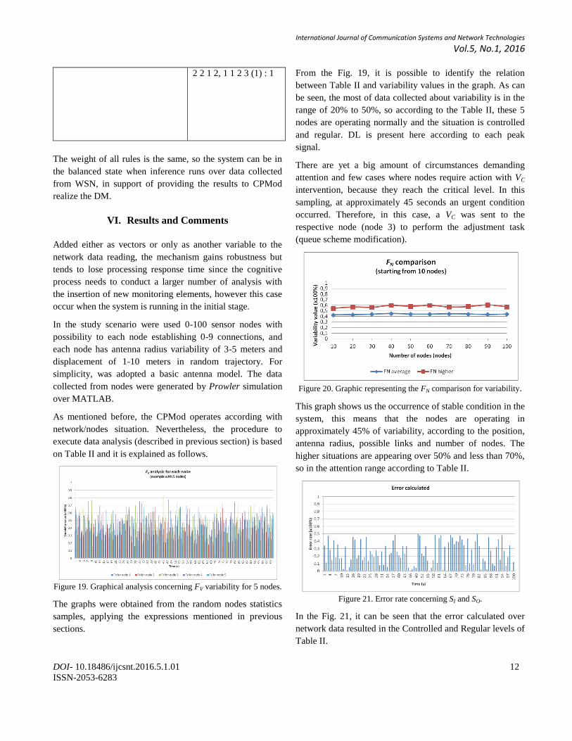
Figure 19. Graphical analysis concerning FV variability for 5 nodes.
The graphs were obtained from the random nodes statistics
samples, applying the expressions mentioned in previous
sections.
From the Fig. 19, it is possible to identify the relation
between Table II and variability values in the graph. As can
be seen, the most of data collected about variability is in the
range of 20% to 50%, so according to the Table II, these 5
nodes are operating normally and the situation is controlled
and regular. DL is present here according to each peak
signal.
There are yet a big amount of circumstances demanding
attention and few cases where nodes require action with VC
intervention, because they reach the critical level. In this
sampling, at approximately 45 seconds an urgent condition
occurred. Therefore, in this case, a VC was sent to the
respective node (node 3) to perform the adjustment task
(queue scheme modification).
Figure 20. Graphic representing the FN comparison for variability.
This graph shows us the occurrence of stable condition in the
system, this means that the nodes are operating in
approximately 45% of variability, according to the position,
antenna radius, possible links and number of nodes. The
higher situations are appearing over 50% and less than 70%,
so in the attention range according to Table II.
Figure 21. Error rate concerning SI and SO.
In the Fig. 21, it can be seen that the error calculated over
network data resulted in the Controlled and Regular levels of
Table II.

International Journal of Communication Systems and Network Technologies
Vol.5, No.1, 2016
DOI- 10.18486/ijcsnt.2016.5.1.01 13
ISSN-2053-6283
Figure 22. VM with tendency line according to the memory status.
From the Fig. 22, is understood that with the network time
running, the memory usage tends to be higher according to
the tendency line. It can be seen that exists 6 peaks
surrounding 80% memory usage, and in that cases VC is sent
to the respective nodes to try corrections in memory, queue
or route tables.
The idea that this mechanism will overload the network with
unnecessary data packets seems reasonable but, when the
sensors/actuators are synchronized within the nodes and
respective features after the initial setting stage, the system
pre-stabilizes and acts according to the alterations done by
the CPMod.
Using FN, VM and Ԑ parameters, the DMp can be executed
according to the Table II to regularize the nodes situations
regarding memory, queue, energy and route adjustments. DL
is obtained too from these parameters and tends to be near to
their higher values, concerning the average relation
described in (16).
The real strictly direct correlation between CPMod process
and QoS assurance is not depicted from the above graphs,
but it will be treated in a sequence work.
With respect to the Fuzzy Logic applied to DM in ACS
architecture, the surfaces of Figs. 23-32 present the specific
analysis surrounding each input-output element, according to
( ) coordinates. In the graphs, X and Y represent input
elements and Z represents the output of Fig. 9.
Figure 23. Surface of Drop x Delay x Memory.
From the Fig. 23, it can be seen that with growing of packets
dropped in network in conjunction with delay to transmit
data end-to-end indicates an elevated necessity for memory
available in nodes, or in other words, the memory will be a
bottleneck for the network soon.
Figure 24. Surface of Drop x Energy x Memory.
The Fig. 24 shows that even with low drop rate of packets, if
energy consumed by nodes raises over 60%, the memory is
also committed.
International Journal of Communication Systems and Network Technologies
Vol.5, No.1, 2016
DOI- 10.18486/ijcsnt.2016.5.1.01 14
ISSN-2053-6283
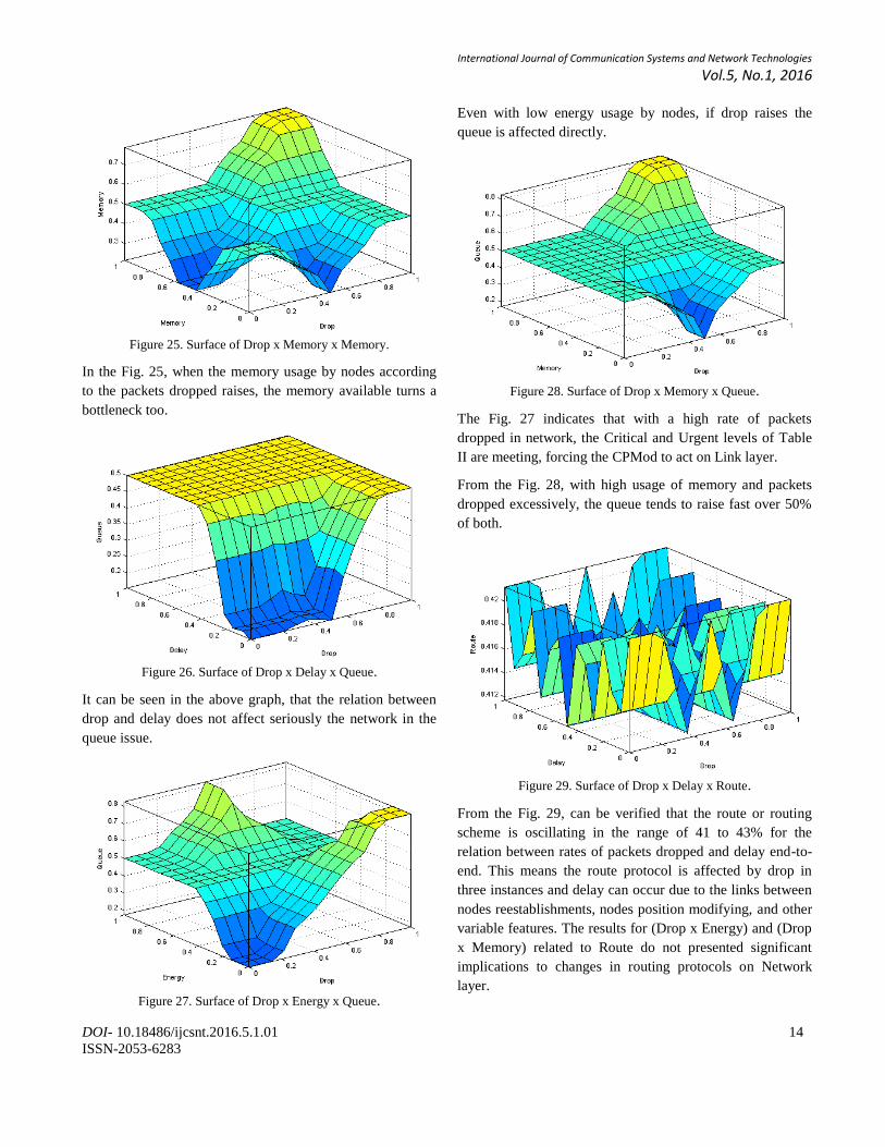
Figure 25. Surface of Drop x Memory x Memory.
In the Fig. 25, when the memory usage by nodes according
to the packets dropped raises, the memory available turns a
bottleneck too.
Figure 26. Surface of Drop x Delay x Queue.
It can be seen in the above graph, that the relation between
drop and delay does not affect seriously the network in the
queue issue.
Figure 27. Surface of Drop x Energy x Queue.
Even with low energy usage by nodes, if drop raises the
queue is affected directly.
Figure 28. Surface of Drop x Memory x Queue.
The Fig. 27 indicates that with a high rate of packets
dropped in network, the Critical and Urgent levels of Table
II are meeting, forcing the CPMod to act on Link layer.
From the Fig. 28, with high usage of memory and packets
dropped excessively, the queue tends to raise fast over 50%
of both.
Figure 29. Surface of Drop x Delay x Route.
From the Fig. 29, can be verified that the route or routing
scheme is oscillating in the range of 41 to 43% for the
relation between rates of packets dropped and delay end-to-
end. This means the route protocol is affected by drop in
three instances and delay can occur due to the links between
nodes reestablishments, nodes position modifying, and other
variable features. The results for (Drop x Energy) and (Drop
x Memory) related to Route do not presented significant
implications to changes in routing protocols on Network
layer.
International Journal of Communication Systems and Network Technologies
Vol.5, No.1, 2016
DOI- 10.18486/ijcsnt.2016.5.1.01 15
ISSN-2053-6283
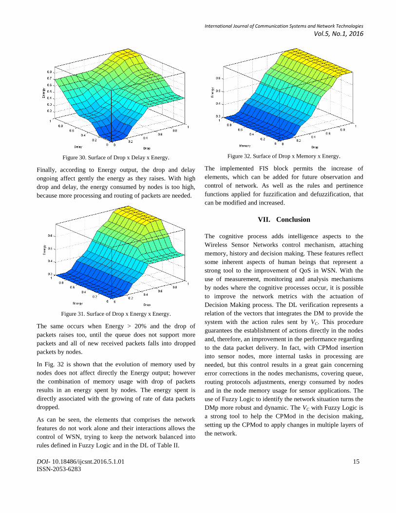
Figure 30. Surface of Drop x Delay x Energy.
Finally, according to Energy output, the drop and delay
ongoing affect gently the energy as they raises. With high
drop and delay, the energy consumed by nodes is too high,
because more processing and routing of packets are needed.
Figure 31. Surface of Drop x Energy x Energy.
The same occurs when Energy > 20% and the drop of
packets raises too, until the queue does not support more
packets and all of new received packets falls into dropped
packets by nodes.
In Fig. 32 is shown that the evolution of memory used by
nodes does not affect directly the Energy output; however
the combination of memory usage with drop of packets
results in an energy spent by nodes. The energy spent is
directly associated with the growing of rate of data packets
dropped.
As can be seen, the elements that comprises the network
features do not work alone and their interactions allows the
control of WSN, trying to keep the network balanced into
rules defined in Fuzzy Logic and in the DL of Table II.
Figure 32. Surface of Drop x Memory x Energy.
The implemented FIS block permits the increase of
elements, which can be added for future observation and
control of network. As well as the rules and pertinence
functions applied for fuzzification and defuzzification, that
can be modified and increased.
VII. Conclusion
The cognitive process adds intelligence aspects to the
Wireless Sensor Networks control mechanism, attaching
memory, history and decision making. These features reflect
some inherent aspects of human beings that represent a
strong tool to the improvement of QoS in WSN. With the
use of measurement, monitoring and analysis mechanisms
by nodes where the cognitive processes occur, it is possible
to improve the network metrics with the actuation of
Decision Making process. The DL verification represents a
relation of the vectors that integrates the DM to provide the
system with the action rules sent by VC. This procedure
guarantees the establishment of actions directly in the nodes
and, therefore, an improvement in the performance regarding
to the data packet delivery. In fact, with CPMod insertion
into sensor nodes, more internal tasks in processing are
needed, but this control results in a great gain concerning
error corrections in the nodes mechanisms, covering queue,
routing protocols adjustments, energy consumed by nodes
and in the node memory usage for sensor applications. The
use of Fuzzy Logic to identify the network situation turns the
DMp more robust and dynamic. The VC with Fuzzy Logic is
a strong tool to help the CPMod in the decision making,
setting up the CPMod to apply changes in multiple layers of
the network.
International Journal of Communication Systems and Network Technologies
Vol.5, No.1, 2016
DOI- 10.18486/ijcsnt.2016.5.1.01 16
ISSN-2053-6283
For future researches some issues should be treated as
follows: more nodes can be inserted into DM analysis, the
feature concerning energy usage can be explored expanding
FN, VM and VC, another control scheme can be defined as
complementary solution for DMp, add more elements in
Fuzzy block for observation and control of network, the
rules and pertinence functions can be modified and
increased, and comparisons with other WSN protocols
concerning control and metrics improvement in the network
point of view.
Acknowledgment
M.S.W. thanks all his coworkers and friends and especially
his wife for participating in the accomplishment of this work
that is a part of his PhD thesis.
This work was supported by Conselho Nacional de
Desenvolvimento Científico e Tecnológico (CNPq) under
Grant 307633/2011-0 and by Fundação de Amparo à
Pesquisa do Estado de São Paulo (FAPESP) under Grant
2012/24789-0.
References
[1] LI, J. et al., “Efficient Traffic Aware Multipath Routing
Algorithm in Cognitive Networks”, Fifth International
Conference on Genetic and Evolutionary Computing
(ICGEC), Xiamen, (2011) September.
[2] ALCARAZ, C. et al., “Wireless Sensor Networks and
the Internet of Things: Do We Need a Complete
Integration?”, Computer Science Department of
University of Malaga, 1st International Workshop on
the Security of the Internet of hings (SecIo ’10),
Tokyo, Japan, (2010) December.
[3] EZREIK, A. and GHERYANI, A., “Design and
Simulation of Wireless Network using NS-2”, 2nd
International Conference on Computer Science and
Information echnology (ICCSI ’2012), Singapore,
(2012) April.
[4] INTANAGONWIWAT, S.; GOVINDAN, R. and
ESTRIN, D., “Directed Diffusion: A Scalable and
Robust Communication Paradigm for Sensor
Networks”, Proceedings of the 6th
annual International
Conference on Mobile Computing and Networking
(MobiCom’2000), Boston, USA, (2000) August 6-11.
[5] SINGH, N.; LAL DUA, R. and MATHUR, V.,
“Network Simulator NS2-2.35”, International Journal
of Advanced Research in Computer Science and
Software Engineering (IJARCSSE), vol. 2, issue 5,
(2012) May, pp. 224-228.
[6] SOMOV, A.; DUPONT, C. and GIAFFREDA, R.,
“Supporting Smart-city Mobility with Cognitive
Internet of Things”, Conference of Future Network &
MobileSummit’2013, International Information
Management Corporation (IIMC), Portugal, Lisboa,
(2013) July.
[7] VIJAY, G.; BDIRA, E. B. A. and IBNKAHLA, M.,
“Cognition in Wireless Sensor Networks: A
Perspective”, IEEE Sensors Journal, vol. 11, n. 3,
(2011) March, pp. 582-592.
[8] WANG, Q., “Traffic Analysis & Modeling in Wireless
Sensor Networks and Their Applications on Network
Optimization and Anomaly Detection”, Macrothink
Institute, Network Protocols and Algorithms, vol. 2, n.
1, Sundsvall, Sweden, (2010), pp. 74-92.
[9] WEI YE et al., “Evaluating Control Strategies for
Wireless-Networked Robots Using an Integrated
Robot and Network Simulation”, Proceedings of the
IEEE International Conference on Robotics and
Automation (ICRA 2001), Seoul, Korea, (2001) May.
[10] ZHANG, N.; GUAN, J. and XU, C., “Traffic
Prediction Model for Cognitive Networks”,
Proceedings of International Conference on Advanced
Intelligence and Awareness Internet (AIAI’2011),
Shenzhen, China, (2011) October.
[11] ZHANG, M. et al., “Cognitive Internet of Things:
Concepts and Application Example”, International
Journal of Computer Science Issues (IJCSI), vol. 9,
issue 6, n. 3, November, (2012), pp. 151-158.
[12] GS omar, ripti Sharma, Brijesh Kumar, “Fuzzy
based Ant colony Optimization Approach for Wireless
Sensor Network”, Wireless Personal Communication,
Vol.84, No.1, pp.361-375, May 2015.
Top Related