


Languages
Pages
Legal

Acceleration Simulation of a Vehicle with a Continuously VariablePower Split Transmission
Zhijian Lu
Thesis submitted to the faculty of the College of Engineering and MineralResources at West Virginia University in partial fulfillment of the
requirements for the degree of
Master of Sciencein
Mechanical Engineering
James Smith, Ph.D., ChairVictor Mucino, Ph.D.
Gregory Thompson, Ph.D.
July 29, 1998
Morgantown, West Virginia
Keywords: CVT, Vehicle Simulation, Transmission
ii
Acceleration Simulation of a Vehicle with a Continuously Variable PowerSplit Transmission
Zhijian Lu
(ABSTRACT)
A continuously variable transmission system has often been considered forautomobiles. It offers the potential to allow the engine to operate at peak efficiencywithout disturbing the driver with discrete shifts. The application of CVTs in automobileshas been attempted for many years. This concept has been rapidly developed in the lasttwenty years. The shaft-to-shaft belt CVT is now the most commonly used CVT productin the automobiles. The main drawback of this kind of CVT is limited torque capacityand the modest power efficiency. This prevents the belt CVT from being used in thevehicles with large displacement engines.
A new concept involves a power split function. A continuously variable powersplit transmission (CVPST) is created by combining a V-belt CVT with a planetary geartrain. The V-belt CVT is used as a control unit. By using this technology, the powerflowing through the belt at low speeds is less than 50 percent. A step-up gearbox is usedto expand the CVPST ratio for the applications in automobiles. The CVPST enhances thetransmission torque capacity and improves the overall transmission efficiency.
This thesis involves the study of the CVPST system. Based on the analysis of thevehicle dynamics and the CVPST system, a computer program is developed. By usingthis program, the CVPST system design can be accomplished. The vehicle accelerationcan be simulated to evaluate the CVPST performance. The acceleration simulation ofvehicles equipped with standard (manual) and automatic transmissions is also possible tobe carried out.
iii
COPYRIGHT 1998
All rights reserved. No part of this book may be reproduced or transmitted in any
form or by any means, electronic or mechanical, including photocopying or by any
information storage and retrieval system, without the written permission of the author,
except where permitted by law.
iv
ACKNOWLEDGEMENTS
I would like to thank Dr. Victor Mucino for his guidance throughout my thesis
work. Also, I would like to extend my gratitude to Dr. Gregory Thompson for his wise
counsel and constructive comments. A special thanks to Dr. James Smith for making
everything possible.
Finally, thanks to my wife, Zhang Shenglan, and my son, Lu Qing, for their love
and faithful support. A special gratefulness to my mother for her love and moral support,
as they were just a phone call away from me.
v
TABLE OF CONTENTS
COPYRIGHT 1998 .......................................................................................................iii
ACKNOWLEDGEMENTS................................................................................................iv
TABLE OF CONTENTS ....................................................................................................v
LIST OF FIGURES..........................................................................................................viii
LIST OF TABLES...............................................................................................................x
LIST OF SYMBOLS..........................................................................................................xi
CHAPTER 1 INTRODUCTION........................................................................................1
CHAPTER 2 LITERATURE REVIEW.............................................................................5
2.1 Continuously Variable Transmission Introduction ...................................................5
2.1.1 All Gear CVT .....................................................................................................6
2.1.2 Traction Type CVT.............................................................................................6
2.1.3 Toroidal Type CVT ............................................................................................7
2.1.4 Hydraulic CVT ...................................................................................................8
2.1.5 Metal-V-Chain (MVC) CVT ..............................................................................8
2.1.6 Flat Belt CVT .....................................................................................................9
2.1.7 V-Belt CVT ........................................................................................................9
2.2 Performance of Metal V-Belt Continuously Variable Transmission ......................11
2.3 Power Split Technology ..........................................................................................12
2.4 Vehicle Drive Simulation ........................................................................................14
2.5 Problem Description and Thesis Objective .............................................................15
CHAPTER 3 VEHICLE DYNAMICS.............................................................................18
3.1 Newton’s Second Law.............................................................................................19
3.2 Dynamic Loads of a Vehicle ...................................................................................20
vi
3.2.1 Traction Force...................................................................................................20
3.2.2 Aerodynamic Drag............................................................................................24
3.2.2.1 Air Density ................................................................................................24
3.2.2.2 Drag Coefficient ........................................................................................25
3.2.2.3 Vehicle Relative Velocity..........................................................................25
3.2.3 Rolling Resistance ............................................................................................26
3.3 Vehicle Acceleration ...............................................................................................28
CHAPTER 4 CONTINUOUSLY VARIABLE POWER SPLIT TRANSMISSION(CVPST) ANALYSIS .....................................................................................30
4.1 Model of Study........................................................................................................30
4.2 System Analysis ......................................................................................................32
4.2.1 CVPST Ratio ....................................................................................................32
4.2.2 Power Split Factor ............................................................................................34
4.2.3 Power Flow.......................................................................................................35
4.3 CVPST System Design............................................................................................37
4.3.1 Determination of rg and rcg ...............................................................................37
4.3.2 Step-up Gear Ratio ...........................................................................................39
4.3.3 Design Example................................................................................................41
CHAPTER 5 SIMULATION EQUATIONS OF VEHICLE ACCELERATION ...........44
5.1 Simulation Equations for Constant Transmission Ratio and Efficiency.................44
5.1.1 Equation Simplification....................................................................................44
5.1.1.1 Engine Torque ...........................................................................................45
5.1.1.2 Rolling Resistance .....................................................................................46
5.1.1.3 Drag Term..................................................................................................46
5.1.2 Solution of the Equation for Constant Ratio and Efficiency ............................47
5.2 Simulation Equations for Variable Transmission Ratio and Efficiency..................48
5.2.1 Shift Velocity....................................................................................................50
5.2.2 Equations for Simulation ..................................................................................51
5.2.2.1 Transmission Ratio ....................................................................................51
5.2.2.2 CVPST Efficiency .....................................................................................51
5.2.3 Differential Equation and Solutions .................................................................53
vii
CHAPTER 6 ACCELERATION SIMULATION RESULTS AND ANALYSIS..........56
6.1 Simulation Conditions .............................................................................................56
6.1.1 Simulation Model .............................................................................................56
6.1.2 Shift Velocity....................................................................................................59
6.1.3 Simulation Assumptions...................................................................................61
6.2 Simulation of Torque–Limited Acceleration with a Standard Transmission..........61
6.2.1 Engine Torque ..................................................................................................61
6.2.2 Parameters for Simulation ................................................................................63
6.2.3 Simulation Results............................................................................................63
6.3 Simulation of Best Fuel Economy Acceleration with an Automatic Transmission 67
6.3.1 Torque Curve....................................................................................................67
6.3.2 Data for Simulation ..........................................................................................68
6.3.3 Simulation Results............................................................................................68
6.4 Acceleration Simulation of a Vehicle with a CVPST .............................................71
6.4.1 Simulation Model .............................................................................................71
6.4.2 Simulation of Stage I ........................................................................................72
6.4.3 Simulation of Stage II and III ...........................................................................73
6.4.4 Simulation Results............................................................................................74
6.5 Discussion of Results ..............................................................................................80
6.6 Conclusion...............................................................................................................82
6.7 Future Recommendations........................................................................................82
REFERENCES..................................................................................................................84
APPENDIX-A PROGRAM FLOW CHART AND CODE FOR SIMULATION ...........88
APPENDIX-B SIMULATION RESULTS OF A VEHICLE WITH A CVPST ..............98
VITA…………................................................................................................................100
viii
LIST OF FIGURES
Figure 1-1 A prototype of CVPST with a step-up gearbox (CK Eng., Canada). ...............3
Figure 2-1 Classification of continuously variable transmissions......................................5
Figure 2-2 V-belt type CVT (Hanses, 1997) ......................................................................9
Figure 2-3 Hybrid V-belt and metal pushing V-belt (Fujii et al, 1992, 1993) .................10
Figure 3-1 SAE vehicle axis system (Gillespie, 1992)....................................................19
Figure 3-2 Arbitrary forces acting on a vehicle (Gillespie, 1992)....................................20
Figure 3-3 Engine torque as a function of throttling valve opening and enginespeed (generated from Fig. 4, Yamaguchi et. al., 1993) .................................21
Figure 3-4 V8 engine (300 in3 ) map (Gillespie, 1992)....................................................22
Figure 3-5 Engine torque as a function of engine speed for five gear sets.......................23
Figure 3-6 Coefficients for determining rolling resistance coefficient by Eq. (3-16)(Gillepie, 1992)................................................................................................27
Figure 4-1 Arrangement of CVT and PGT.......................................................................30
Figure 4-2 Specific power low of Input-coupled type......................................................31
Figure 4-3 Specific power flow of Output-coupled type..................................................31
Figure 4-4 A basic CVPST system (Mucino et al, 1997).................................................32
Figure 4-5 An idealized planetary system ........................................................................33
Figure 5-1 Power Loss of CVT as a Function of Variator Ratio (by PhilippeArques) ............................................................................................................52
Figure 5-2 CVPST efficiency as a function of variator ratio ..........................................52
Figure 6-1 Simulation model of vehicle with standard or automatic transmission ..........57
Figure 6-2 Simulation model of a CVPST with a step-up gearbox..................................57
Figure 6-3 Characteristics of the engine for the simulation (Yamaguchi et. al.,1993)................................................................................................................58
Figure 6-4 Engine speed-vehicle velocity chart ...............................................................60
Figure 6-5 The maximum torque curve of the engine .......................................................62
Figure 6-6 General input data form for simulation...........................................................62
Figure 6-7 Multi-ratio transmission input data form........................................................63
Figure 6-8 Simulation result of a vehicle with a 5-speed transmission (TLA) ................64
Figure 6-9 (a) Vehicle velocity as a function of time (Standard, TLA) ............................65
Figure 6-9 (b) Vehicle acceleration as a function of time (Standard, TLA) .....................65
ix
Figure 6-9 (c) Vehicle displacement as a function of time (Standard, TLA)....................66
Figure 6-9 (d) Transmission ratio as a function of time (Standard, TLA) ........................66
Figure 6-10 Shift schedule for best fuel economy (Yamaguchi et. al.,1993)....................67
Figure 6-11 Fitted engine torque curves for BFEA..........................................................68
Figure 6-12 Transmission input data of an automatic transmission for BFEA................69
Figure 6-13 (a) Vehicle velocity as a function of time (Automatic, BFEA) ....................69
Figure 6-13 (b) Vehicle acceleration as a function of time (Automatic, BFEA) ..............70
Figure 6-13 (c) Vehicle displacement as a function of time (Automatic, BFEA)............70
Figure 6-14 Simulation results of a vehicle with an automatic transmission (BFEA) .....71
Figure 6-15 Simulation model of vehicles with a CVPST ...............................................72
Figure 6-16 Transmission input data form for CVPST ....................................................73
Figure 6-17 Engine speed-vehicle velocity chart for CVPST ..........................................74
Figure 6-18 Simulation results of torque-limited acceleration (TLA) with CVPST........75
Figure 6-19 Transmission ratio as a function of time (CVPST, TLA).............................76
Figure 6-20 (a) Vehicle velocity as a function of time (CVPST, TLA)..........................76
Figure 6-20 (b) Vehicle acceleration as a function of time (CVPST, TLA) ....................77
Figure 6-21 Transmission ratio as a function of time (CVPST, BFEA) ..........................77
Figure 6-22 (a) Vehicle velocity as a function of time (CVPST, BFEA) ........................78
Figure 6-22 (b) Vehicle acceleration as a function of time (CVPST, BFEA)..................78
Figure 6-23 Power flowing through the belt and gear as functions of variator ratio ........79
x
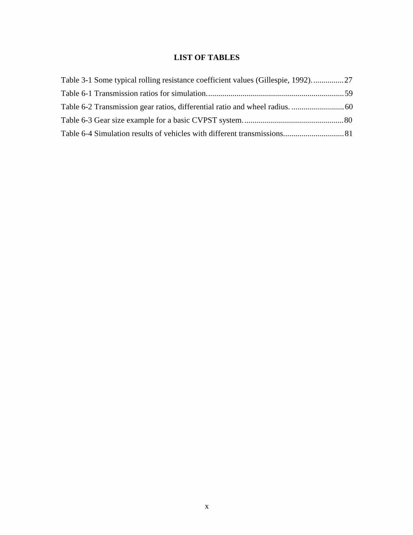
LIST OF TABLES
Table 3-1 Some typical rolling resistance coefficient values (Gillespie, 1992). ...............27
Table 6-1 Transmission ratios for simulation....................................................................59
Table 6-2 Transmission gear ratios, differential ratio and wheel radius. ..........................60
Table 6-3 Gear size example for a basic CVPST system. .................................................80
Table 6-4 Simulation results of vehicles with different transmissions..............................81
xi
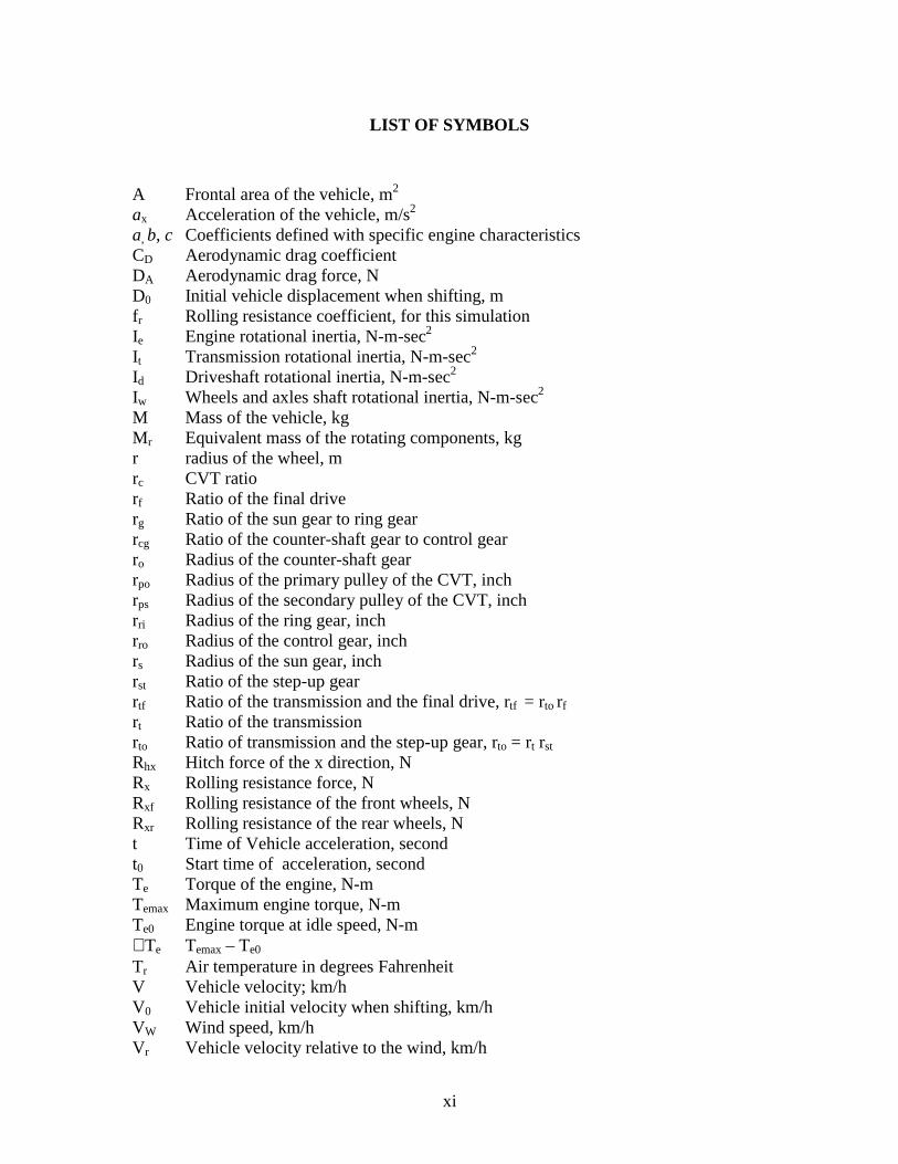
LIST OF SYMBOLS
A Frontal area of the vehicle, m2
ax Acceleration of the vehicle, m/s2
a, b, c Coefficients defined with specific engine characteristicsCD Aerodynamic drag coefficientDA Aerodynamic drag force, ND0 Initial vehicle displacement when shifting, mfr Rolling resistance coefficient, for this simulationIe Engine rotational inertia, N-m-sec2
It Transmission rotational inertia, N-m-sec2
Id Driveshaft rotational inertia, N-m-sec2
Iw Wheels and axles shaft rotational inertia, N-m-sec2
M Mass of the vehicle, kgMr Equivalent mass of the rotating components, kgr radius of the wheel, mrc CVT ratiorf Ratio of the final driverg Ratio of the sun gear to ring gearrcg Ratio of the counter-shaft gear to control gearro Radius of the counter-shaft gearrpo Radius of the primary pulley of the CVT, inchrps Radius of the secondary pulley of the CVT, inchrri Radius of the ring gear, inchrro Radius of the control gear, inchrs Radius of the sun gear, inchrst Ratio of the step-up gearrtf Ratio of the transmission and the final drive, rtf = rto rf
rt Ratio of the transmissionrto Ratio of transmission and the step-up gear, rto = rt rst
Rhx Hitch force of the x direction, NRx Rolling resistance force, NRxf Rolling resistance of the front wheels, NRxr Rolling resistance of the rear wheels, Nt Time of Vehicle acceleration, secondt0 Start time of acceleration, second Te Torque of the engine, N-mTemax Maximum engine torque, N-mTe0 Engine torque at idle speed, N-m∇Te Temax – Te0
Tr Air temperature in degrees FahrenheitV Vehicle velocity; km/hV0 Vehicle initial velocity when shifting, km/hVW Wind speed, km/hVr Vehicle velocity relative to the wind, km/h
xii
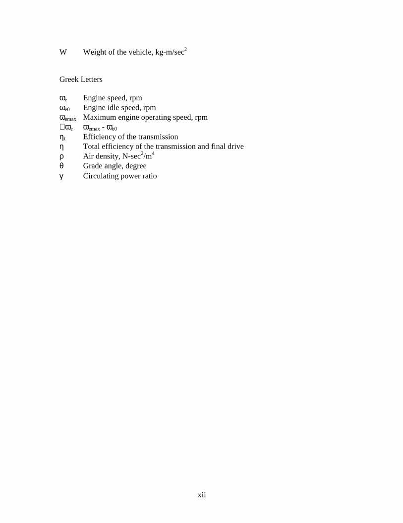
W Weight of the vehicle, kg-m/sec2
Greek Letters
ωe Engine speed, rpmωe0 Engine idle speed, rpmωemax Maximum engine operating speed, rpm∇ωe ωemax - ωe0
ηt Efficiency of the transmissionη Total efficiency of the transmission and final driveρ Air density, N-sec2/m4
θ Grade angle, degreeγ Circulating power ratio
1
CHAPTER 1 INTRODUCTION
A continuously variable transmission (CVT) provides a continuously variable
ratio between the power source of a vehicle and its wheels. CVT offers the potential to
allow the engine to operate at peak efficiency without disturbing the customer with
discrete shifts. For many years, CVTs have been considered by many as the next step in
the evolution of the automatic transmission. Incorporating CVTs in automobiles has been
attempted for many years. Almost every generation of automobile engineers has tried to
equip automobiles with CVT.
A century ago a rubber V-belt transmission was used in Benz and Daimler
gasoline-engine-powered vehicles. A very important development of CVT was the so-
called Variomatic in 1965 (Hendriks et. al., 1988). One million Volvo cars have been
equipped with this kind of transmission since the year 1975. The capacity of such a CVT
is limited by the power capacity of the weakest part, in this case, its rubber belt.
To enhance the CVT’s capacity, efficiency, and durability, many different kinds
of CVT have been developed in the past twenty years. Of all CVT’s, the metal pushing
block V-belt (MVB) CVT is the most important development. It has received very good
compactness values or power density values and higher power efficiency figures than
other types of traction, hydraulic, or electric CVTs (Hendriks et al., 1988).
MVB CVT has been equipped more than one million Japanese and European cars
since its development (Ashley, 1994). Of all the applications of CVTs in automobiles, 99
percent are found in Japan and Europe. Only about 1 percent is found in U.S. market.
These U.S. cars include the Honda Civic Hx and the Subaru Justy. The reason CVT is not
popularly used in the U.S. is that torque capacity limitations have restricted the
2
production of CVT applications to vehicles with very small displacement engines, 1.6 l or
less, while the top three selling vehicles in this country all have displacements of 3.0 l or
greater.
The present shaft-to-shaft CVT does not offer enough torque capacity. The
modest power efficiency of variable speed units, as compared to straight gears, is another
main reason that the CVT is not widely used (Guebeli et. al., 1993). Under dynamic
running conditions with a very low load at 35 km/h, the shaft-to-shaft CVT’s efficiency is
only 74 percent, while at the higher load of 90 km/h it reaches 90 percent (Bonthron,
1985).
In order to take advantage of the belt CVT and overcome its disadvantages, the
belt CVT conjugated with a gear train was invented (Lemmens, 1972, 1974, Takayama et
al., 1991). The newest development is the continuously variable power split transmission
(CVPST) which combines a planetary gear train with a V-belt CVT (Cowan, 1992,
Mucino et al.,1995, 1997). Two prototypes of CVPST were presented by CK Engineering
at TOPTEC-98 SAE Conference in Southfield, Michigan.
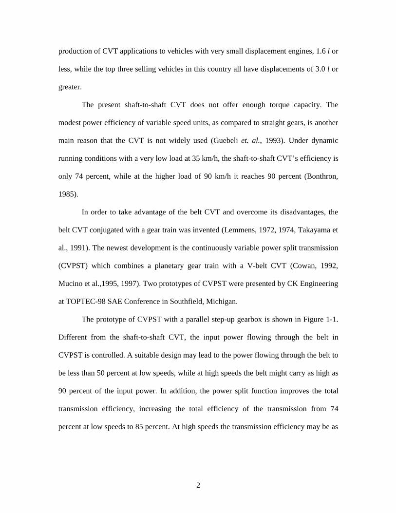
The prototype of CVPST with a parallel step-up gearbox is shown in Figure 1-1.
Different from the shaft-to-shaft CVT, the input power flowing through the belt in
CVPST is controlled. A suitable design may lead to the power flowing through the belt to
be less than 50 percent at low speeds, while at high speeds the belt might carry as high as
90 percent of the input power. In addition, the power split function improves the total
transmission efficiency, increasing the total efficiency of the transmission from 74
percent at low speeds to 85 percent. At high speeds the transmission efficiency may be as
3
high as 93 percent. The power split function expands the application opportunity of
CVTs, enabling the CVT to be incorporated in vehicles with large displacement engines.
Step-up gear sets
Planetary gear train
Belt drive as control gear set
V-belt CVT
Figure 1-1 A prototype of CVPST with a step-up gearbox (CK Eng., Canada).
The CVT currently used in small engine vehicles employs a metal pushing belt.
This kind of belt involves about 300 blocks and ten layers of bands. It is difficult to
manufacture and is thus very expensive (Hendriks et al., 1988). CVPST also promises to
use a rubber belt to replace the metal pushing belt for vehicles with small engines and
further to reduce the cost of the transmission.
CVPST for automotive applications was studied by Mucino et al. (1997). There
are several key parameters involved in the design of the CVPST. For a given vehicle and
a given engine, it is possible to choose suitable parameters for the CVPST to allow the
input power to split and flow through the gear and the belt as desired. Currently, there is
4
not a simulation package available for the acceleration simulation of a vehicle with a
CVPST. Based on the analysis of vehicle dynamics and the CVPST system, this thesis
work involves the acceleration performance simulation of vehicles equipped with a
CVPST. A computer program is developed to accomplish the CVPST system design
based on certain requirements, such as the power capacity of the belt and the overall ratio
of the transmission. In order to evaluate CVPST driveability, the computer program can
then complete the drive test and simulation of the designed CVPST for given engine
characteristics and a specific vehicle body. Using this package, acceleration simulations
of vehicles with standard or automatic transmissions can also be carried out and the
acceleration performance of different transmissions can be compared.
5
CHAPTER 2 LITERATURE REVIEW
2.1 Continuously Variable Transmission Introduction
Transmission systems used in vehicles can be grouped into two main types: step
and stepless ratio transmissions. The traditional multi-ratio transmissions, standard and
automatic, are both step ratio transmissions and have been widely familiar to people. The
continuously variable speed transmission (CVT) is relatively less familiar. Since the first
generation of CVT was used in the automotive industry in 1886, CVT development never
stopped. In the past twenty years, the development of the CVT includes all-gear,
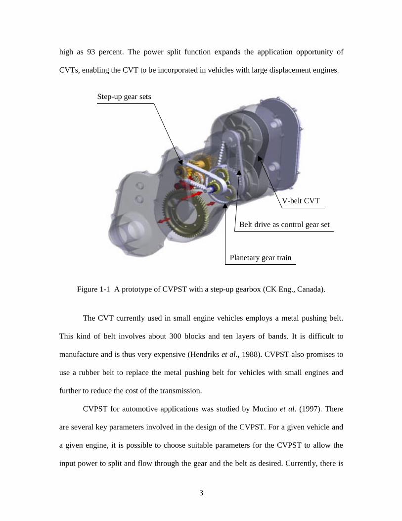
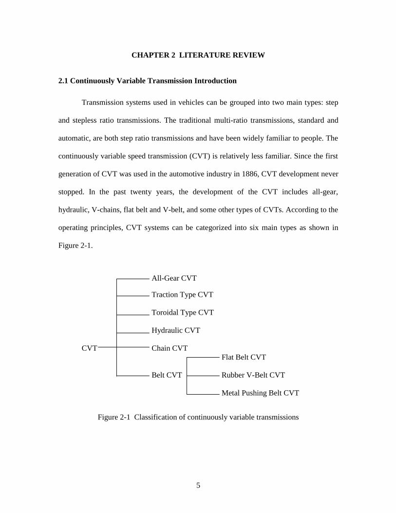
hydraulic, V-chains, flat belt and V-belt, and some other types of CVTs. According to the
operating principles, CVT systems can be categorized into six main types as shown in
Figure 2-1.
All-Gear CVT
Traction Type CVT
Toroidal Type CVT
Hydraulic CVT
CVT Chain CVTFlat Belt CVT
Belt CVT Rubber V-Belt CVT
Metal Pushing Belt CVT
Figure 2-1 Classification of continuously variable transmissions
6
2.1.1 All Gear CVT
An all gear CVT provides the continuous variable speed ratio by gear trains. This
mechanism is capable of producing a wide range of speed outputs, including very high
torque at low speed and very high speed at low torque. Cook (1975) invented an all gear
CVT which was different from many prior automatic transmissions requiring complex
fluid logic control. It is controlled by the input and output torque. The output shaft is
driven through both the input and intermediate shafts. A power source such as the
automobile engine is connected through a clutch to the transmission input shaft. A load
such as the automobile’s drive shaft is connected to the output shaft. At low engine
speeds, it provides the highest gear ratio. When the output torque reduces to a certain
level, all drive power is provided by the planetary gear train. Won (1989) disclosed
another all gear CVT completing gear ratio change by a combination of floating gearing
and differential gearing.
Epilogic, Inc. developed a fully geared CVT with a continuous variable ratio
range of 1:1 to 1:4 (Fitz and Pires, 1991). The target application was electric vehicles.
The ratio adjustment can be controlled with a simple, servo-driven actuator. The ratio
adjustment varies linearly with the control actuator displacement.
2.1.2 Traction Type CVT
Continuously variable traction roller transmissions include a continuously
variable transmission unit having an input disc, an output disc, and a pair of traction
rollers. The traction rollers come in frictional contact with the two discs and perform
control of a gear ratio by altering the contact state between the two discs and the traction
rollers. An extremely high contact force allows the rollers to transmit considerable power
7
without slippage. Tilting the rollers changes the drive ratio between the disks. The drive
is capable of an efficiency of over 98% at full forward and 80% in full reverse with
power ratings of several hundred horsepower (Hibi, 1993).
The earlier traction roller type CVT is difficult to adjust and screen the loading
nut at the same time in order to obtain a predetermined clearance between the disc
member. In addition, a preload of the disc spring is difficult to set to a constant value due
to susceptible variations in adjusting operation. A new patent (Hibi, 1993) solved these
problems, however, the high cost of the required high strength materials limits its
application. Continuous operation of the traction type transmission at a constant speed
ratio often leads to wear of the toroidal discs and subsequent control difficulties.
2.1.3 Toroidal Type CVT
A toroidal type CVT (Tanaka and Imanishi, 1994) consists of an input disk,
output disk and power rollers. The input disk is attached to an input shaft while the output
disk is fixed to an end of the output shaft. Trunnions are swung around respective pivot
axes transverse to the input shaft and the output shaft and are mounted on a support
bracket arranged on an inner surface of a casing or in the casing in which the toroidal
type CVT is housed. Power rollers are held between the input disk and the output disk. A
loading cam-type pressure device is provided between the input shaft and the input disk
to resiliently urge the input disk to the output disk. The pressure device comprises a cam
plate which rotates with the input shaft and a plurality of rollers held by a holder. The
rollers are rotatable around an axis which is radial to the center of the input shaft. When
the cam plate is rotated with the rotation of input shaft, the rollers are urged to the outer
cam surface of the input disk and the input disk is urged to the power rollers. The input
8
disk is rotated by the engagement of the pair of cam surfaces and the rollers. The rotation
of the input disk is transmitted to the output disk through the power rollers, so that the
output shaft fixed to the output disk is rotated. The ratio change is completed by swing
trunnions to incline a displaceable shaft so that the power rollers abut against the different
portion of the concave surfaces of the input and output shafts.
2.1.4 Hydraulic CVT
Hydraulic CVTs provide a continuously variable speed ratio by adjusting the
hydraulic motor speed. This involves the adjustment of the amount of hydraulic fluid in
the closed circuit. For a hydraulic CVT, either the hydraulic pump or the hydraulic motor
or both, are of the variable displacement type (Kawahara et al., 1990, Inoue, 1990,
Furnmoto et al., 1990). The speed ratio of this kind of CVTs is continuously variable
from forward to full reverse. The general large size requirement, high noise, low
efficiency and cost make this type of CVT unsuitable for automotive applications
(Kumm, 1991).
2.1.5 Metal-V-Chain (MVC) CVT
Common in all designs for MVC CVT is a set of fixed sheaves with opposing
movable sheaves, one for the input and one for the output shafts (Avramidis, 1986). The
power is transmitted from input to output shaft by a flexible steel chain. The continuously
variable speed ratio results from moving one set of sheaves together while allowing the
other set of sheaves to be forced apart, thus forcing the steel chain radially outward in one
sheave while inward in the other sheave. This changes the pitch diameters of the two
sheaves and results in stepless ratio change. The torque transmitting mechanism is
friction. Hence, the chain is actually a chain-type metal belt.
9
2.1.6 Flat Belt CVT
The Flat Belt CVT comprises two rotary disk assemblies. One of the assembles is
driven with an input shaft, and the other drives an output shaft to which varying loads
may be applied. The torque is transmitted from the input shaft to the output shaft by an
endless flat belt. There are contact pads located within slots in each of the disk
assemblies. The contact pads form two circles on which the flat belt rides. The
continuously variable diameter with respect to the center of each disk assembly produces
a continuously variable speed ratio (Kumm, 1986).
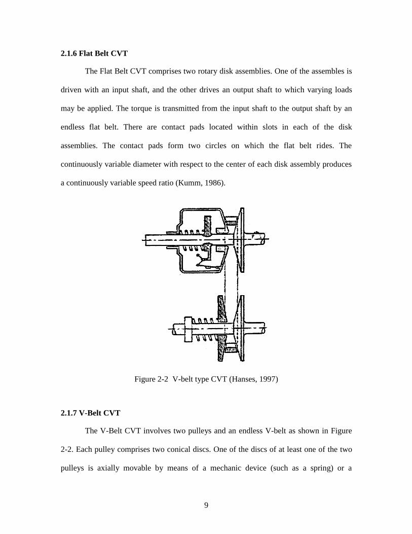
Figure 2-2 V-belt type CVT (Hanses, 1997)
2.1.7 V-Belt CVT
The V-Belt CVT involves two pulleys and an endless V-belt as shown in Figure
2-2. Each pulley comprises two conical discs. One of the discs of at least one of the two
pulleys is axially movable by means of a mechanic device (such as a spring) or a
10
hydraulic control cylinder. The continuously variable transmission ratio is available due
to the motion of the axially movable disc(s), which changes the radii on which the belt
rides. The simplest V-belt CVT is like the one introduced by Hendriks (1991). Most
recent developments of V-belt CVTs comprise a gear train. V-belt CVTs can be divided
into two groups according to whether the belt drive is subjected to the total input power.
The V-belt CVTs, in which the input power of the transmission totally passes through
(Moroto et al., 1986, Kawamoto, 1985, Robbins, 1993), usually have limited torque
transferring capacity. They are used for low power situations. To enhance the belt
capacity, Metal-V-Belt (MVB) (Hendriks et al., 1988) and dry hybrid-V-belt (HVB)
(Fujii et al., 1992, Yuki et al., 1995,) have been developed.
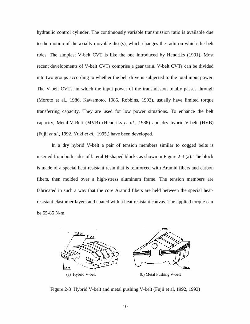
In a dry hybrid V-belt a pair of tension members similar to cogged belts is
inserted from both sides of lateral H-shaped blocks as shown in Figure 2-3 (a). The block
is made of a special heat-resistant resin that is reinforced with Aramid fibers and carbon
fibers, then molded over a high-stress aluminum frame. The tension members are
fabricated in such a way that the core Aramid fibers are held between the special heat-
resistant elastomer layers and coated with a heat resistant canvas. The applied torque can
be 55-85 N-m.
(a) Hybrid V-belt (b) Metal Pushing V-belt
Figure 2-3 Hybrid V-belt and metal pushing V-belt (Fujii et al, 1992, 1993)
11
The MVB was developed by Van Doorne’s Transmissie B. V. (VDT) in the
1980s. A complete belt unit consists of about 300 blocks connected by two sets of 10
steel bands inserted in the two sides of the metal blocks as shown in Figure 2-3 (b). The
multiple layers of the steel bands provide pretension forces, which correctly guides the
elements along the straight path between the two pulleys. Torque is transmitted from the
drive pulley to the driven pulley by compression between the blocks. Because it attains
very good compactness or power density values, MVB is the sole belt used for shaft-to-
shaft CVTs at present in vehicle applications. The standard metal pushing belt is being
applied in an engine range from 550 cc to 1.2 liter (Hendriks et. al., 1988). It is working
well for small cars. However, the metal pushing belt is very expensive due to the
difficulty in manufacturing. Also, the capacity of the belt is still not sufficient for the
shaft-to-shaft CVTs to be used for vehicles with large displacement engines.
2.2 Performance of Metal V-Belt Continuously Variable Transmission
The study of the performance of CVTs with MVB began early in the 1980’s. It
has been found that at the wider ratio range the CVT indicates an improvement in fuel
economy. Due to the use of a CVT, vehicle power can be controlled along an ideal engine
torque-speed line, which gives the best fuel consumption and emission characteristics for
all power demands of the vehicle. Thus, the engine efficiency could be improved by an
average of 30 percent over the city cycle and by 30 to 40 percent on highway cruise (Guo
et. al., 1988). Ishibash et al. (1989) reported that the optimized combination of the two-
stroke cycle engine and the CVT with other improvements enables fuel consumption to
be reduced by approximately 30 percent. However, if the CVT efficiency drops 5 percent,
this advantage is lost (Chana, 1986).
12
There were a few studies on the efficiency of the V-belt CVTs. Palmer and Bear
(1977) measured the efficiency of a CVT under various operating conditions such as the
variation in speeds, power outputs and speed ratios. It was found that the average CVT
efficiency was about 80 to 90 percent. A similar experiment was conducted by Bent
(1981), in which a relation between the axial force and the transmission efficiency was
determined. Under the dynamic operation condition, Bonthron (1985) found that the V-
belt CVT efficiency at low speeds was only 74 percent. The overall efficiency, speed loss
and torque loss of the CVT were measured by Chen et al. (1995). The results show that
the efficiency increases with an increase in external loads and is independent of the speed
variation.
2.3 Power Split Technology
Lemmens (1972) described combining a planetary gear train with a V-belt CVT to
produce a transmission. The input shaft is rotated by the power source. The input shaft
rotates drive pulleys of both the V-belt and the chain drive. The chain drive transmits the
rotation to the planetary carrier, while the V-belt transmits to the sun gear. The output
shaft of the transmission is the ring gear. The majority of the power is carried by the
planetary gear train, while the continuously variable V-belt drive is used to control the
speed of the sun gear to gain a neutral setting and an infinitely variable range of both
forward and reverse speeds. The power flowing through the V-belt is thus a reduced
reaction and is kept low. The same inventor improved his invention (Lemmens, 1974) to
provide a continuously variable fully automatic transmission by which the only manual
setting required is the choice among neutral, forward and reverse. This arrangement may
lead to power recirculation, and therefore it is not a real power split system.
13
Takayama et. al. (1989) presented a power split transmission which consists of a
V-belt type CVT and a two-way differential clutch. The power from the engine is
transmitted to the input shaft of the transmission. Two paths are operable to transmit the
power from the input shaft to the output shaft. The main power transmitting path is the
belt while the sub path is through the two-way differential clutch. When the CVT is near
the maximum ratio, the rotating speed of the output gear in the two-way differential
clutch becomes slower than that of the output gear. As a result, the output pulley shaft
obtains the power from the sub power path in addition to the power of the main path. It
becomes possible to increase driving power, and thus the acceleration force, and also to
decrease the load carried by the belt. Using this construction, the overall transmission
capacity is increased and the weight is decreased because of reducing the numbers of
clutches. Because the belt carries the most input power, this proposed arrangement is less
than optimum.
The combination of a flat belt CVT and a normal planetary mechanism was
presented in 1991 (Kumm, 1991). This system enhances the capacity and the efficiency
of the flat belt CVT and provides the reverse capability. In the low speed mode, the input
power is divided into two paths: the first path through the planetary gearing to the output
and a second path from the planetary gearing through the CVT back to the input shaft. In
the high speed mode, a clutch on the shafting from the planetary ring gear to the output
shaft is disengaged and another clutch is engaged. This permits the input power to be
transmitted directly through the CVT to the output shaft. Reverse output speeds are made
available by changing the radius ratio control direction in the CVT when in the low speed
14
mode without actuating the clutches. This arrangement eliminates the capacity limits of
the belt, but the torque transmitted by the gear train is greater than the input torque.
A variable speed transmission unit (any type) connected with a planetary gear
train was proposed by Cowan (1992, 1993). According to his invention, the sun gear and
the primary variator are mounted on the input shaft. The output shaft is connected to the
planetary carrier. There is a counter-shaft on which the secondary variator is mounted. A
counter-shaft gear is meshed with a control gear which is connected to the ring gear.
When the control gear is meshed with the counter-shaft gear through one or any odd
number of intermediate gears and/or high torque belts or chains (allowing the ring gear
and the counter-shaft gear to rotate in the same direction), the input power is split into
two paths. Part of the power flows through the variators then through the counter-shaft
gear to the ring gear. The rest goes directly through the sun gear. As a result, less power
is transmitted by the variator system. If a V-belt CVT is used as the variable speed
transmission unit, it is possible to achieve a function such that for a large input power
only a fraction of the total input power load is transmitted through the belt. This proposal
also exhibits the possibility that the function is achieved with a limited variator ratio
range, which enables the most mechanically efficient ratio range to be selected.
2.4 Vehicle Drive Simulation
The fuel economy of automobiles equipped with hydromechanical transmissions
was studied by simulation (Orshansky et. al., 1974). The simulation results showed that
significant improvements in fuel economy were abtainable by using a CVT to allow the
engine to operate close to best conditions. A program was developed to simulate the
powertrain for fuel economy and performance of a 5 ton truck equipped with a diesel
15
engine in 1988 (Phillips et. al., 1990). This program was further developed for general
purpose vehicle powertrain simulation. It can be used for vehicles equipped with standard
and automatic transmissions. A new development is the vehicle acceleration simulation
program appearing in the web site (Bowling, 1997). This program can be executed from
the internet to simulate the acceleration performance of a vehicle with an automatic
transmission. Due to the restriction of the software, it only can use linear torque curve for
simulation. Currently, there is not a package developed for the acceleration simulation of
a vehicle equipped with a continuously variable power split transmission.
2.5 Problem Description and Thesis Objective
CVTs are not widely accepted by the US market. Part of the reason is that CVTs
in production today do not exploit their theoretical fuel-saving potential (Schwab, 1990).
The problem may include a ratio rate of change lower than required, an optimized control
not achieved and an unconventionally heavier transmission (Thompson, 1992). In fact,
the most important point is that the capacity of the shaft-to-shaft CVTs is too low and the
overall efficiency of this kind of CVT needs improvement. Increasing the size of the belt
and transmission will diminish current CVT’s packaging advantages. The newly
developed CVTs need to provide greater capacity, higher efficiency and better response
(Nakano, 1992).
A V-belt CVT combined with a planetary gear train (PGT) provides a power split
technology as described by Cowan (1992, 1993) and Mucino et al. (1995, 1997) and
produces a continuously variable power split transmission (CVPST) system. This
technology makes it possible to design a system in which the power flowing through the
belt unit is controlled. Only part of the total input power is transmitted by the belt at low
16
speeds, while at high speeds the belt may transmit most of the input power. The output
torque obtained through the planetary output shaft is greater than the torque circulating
through the pulleys. This feature accomplishes two things: first the gear sizes required to
attain variable velocity ratios need not change due to the CVT connection between the
gear train and the output shaft; second, the belt capacity no longer limits the maximum
torque capacity of the system. Hence, the CVPST may enhance the transmission capacity
to enable the V-belt CVT to be used for vehicles with large displacement engines. For a
small vehicle, the CVPST makes it possible to use a regular rubber V-belt as a substitute
for the heavy and expensive metal pushing belt. The CVPST can also improve the total
transmission efficiency because only part of the power flows through the belt at low
speeds and the most efficient variator ratio range is selected. CVPST combined with a
step-up gearbox may expand the overall transmission ratio to a practically useful range
for the applications in automobiles. It promises to keep V-belt CVT’s advantages and to
overcome its drawbacks.
For a given engine map and a given vehicle body, a careful design must be done
to accomplish the power split function. This involves a CVPST parameter determination.
A practically useful CVPST should also result in good driveability and acceleration
performance. This thesis considers a CVPST system consisting of a V-belt CVT (hybrid
belt or metal pushing belt) and a planetary gear train plus a step-up gearbox. The
objective of this thesis work is the analysis of vehicle dynamics and the CVPST system,
and to develop a computer program to predict the following:
• CVPST system design based on the given conditions such as the belt power capacity
and the overall transmission ratio range;
17
• Dynamic drive test and acceleration simulation of a vehicle equipped with a CVPST
and a multi-ratio standard or automatic transmission; and
• Evaluation of the driveability and acceleration performance of a CVPST compared to
standard and automatic transmissions.
18
CHAPTER 3 VEHICLE DYNAMICS
A motor vehicle consists of many components distributed within its exterior
envelope. For acceleration, braking, and most turning analysis, the whole vehicle is often
treated as a lumped mass, except for the wheels. This lumped mass representing the body
is called the sprung mass while the wheels are denoted as unsprung masses. The vehicle
represented by the lumped mass is treated as a mass concentrated at its center of gravity
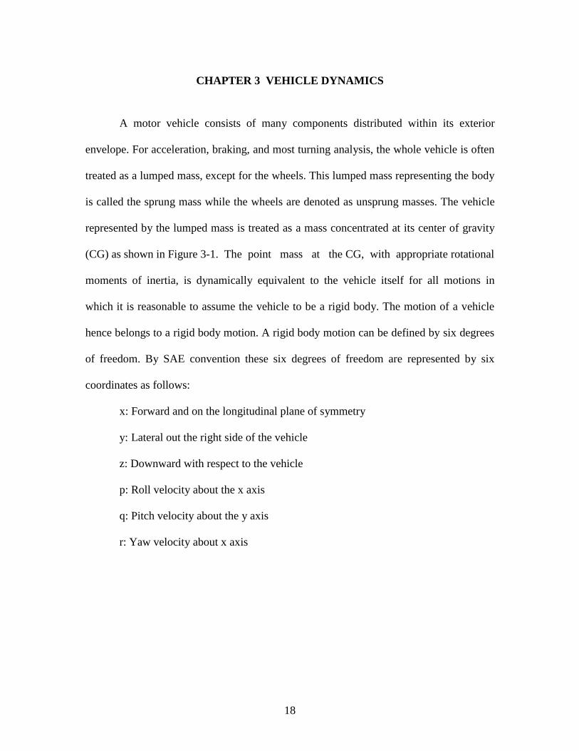
(CG) as shown in Figure 3-1. The point mass at the CG, with appropriate rotational
moments of inertia, is dynamically equivalent to the vehicle itself for all motions in
which it is reasonable to assume the vehicle to be a rigid body. The motion of a vehicle
hence belongs to a rigid body motion. A rigid body motion can be defined by six degrees
of freedom. By SAE convention these six degrees of freedom are represented by six
coordinates as follows:
x: Forward and on the longitudinal plane of symmetry
y: Lateral out the right side of the vehicle
z: Downward with respect to the vehicle
p: Roll velocity about the x axis
q: Pitch velocity about the y axis
r: Yaw velocity about x axis
19
Figure 3-1 SAE vehicle axis system (Gillespie, 1992)
Vehicle motion is usually described with the velocities (forward, lateral, vertical,
roll, pitch and yaw) with respect to the vehicle fixed coordinate system, where the
velocities are referenced to the earth’s fixed coordinate system. The earth’s fixed
coordinate system is normally selected to coincide with the vehicle’s fixed coordinate
system at the point where the maneuver is started. For the purpose of a drive test of a
vehicle used for the evaluation of different transmissions, it is sufficient to consider only
forward or longitudinal motion. The simulation of the vehicle in this paper is therefore
focused on the x direction to test the characteristics of the CVPST in comparison to
standard transmissions.
3.1 Newton’s Second Law
The fundamental law from which most vehicle analysis begins is Newton’s
Second Law. For the translational system in the x direction, the sum of the external forces
acting on the vehicle in this direction is equal to the product of the vehicle mass and the
acceleration in the x direction, i. e.,
xx MaF =∑ (3-1)
20
For the rotational system, the sum of the torques acting on a body about a given
axis is equal to the product of its rotational moment of inertia and the rotational
acceleration about the axis, i. e.,
∑ = αIT (3-2)
3.2 Dynamic Loads of a Vehicle
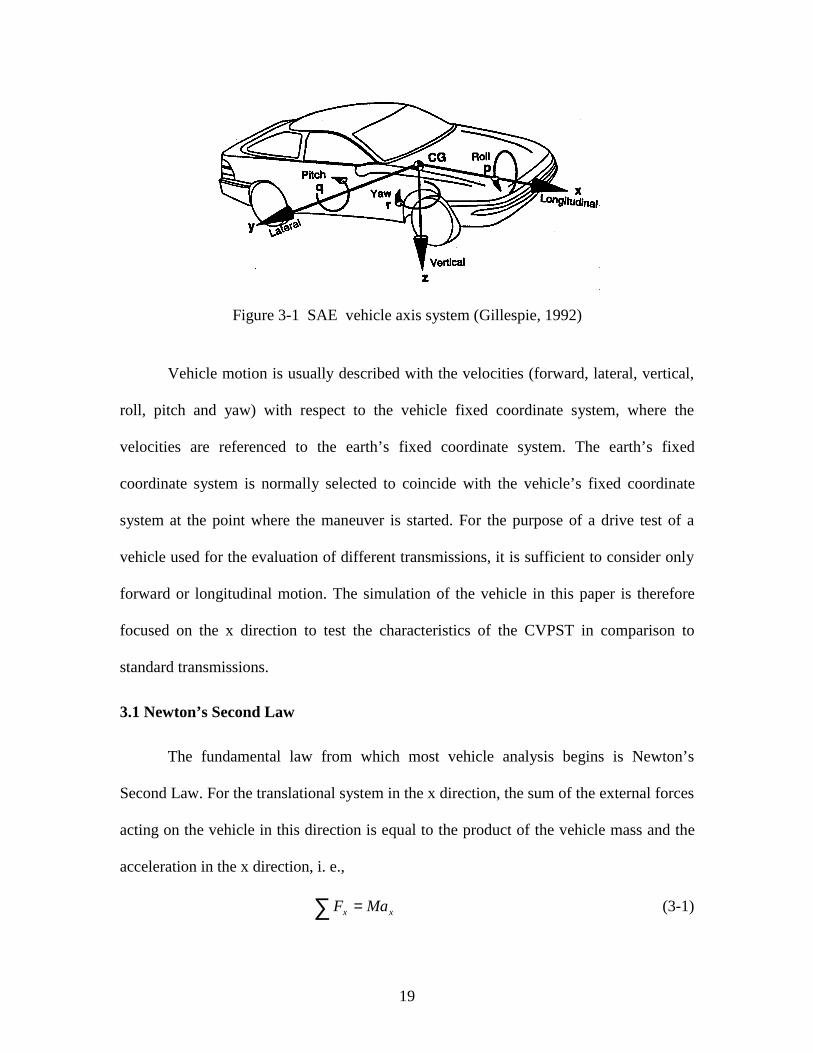
The arbitrary dynamic loads acting on a vehicle in the x-z plane are illustrated in
Figure 3-2. Among all these forces, Fxf and Fxr are traction forces, which push the vehicle
to move forward along the x direction. The rest of the forces in the x directio are road
resistance forces.
Figure 3-2 Arbitrary forces acting on a vehicle (Gillespie, 1992)
3.2.1 Traction Force
The traction force required to drive a vehicle comes from the engine. The engine
torque is transferred to the wheels through the power train. The traction force can be
calculated as:
( )[ ]2
22
r
aIrIrII
r
rTF x
wfdtftetfe
x +++−=η
(3-3)
21
The first term of the right-hand side of Eq. (3-3) is the traction force produced by
the engine. It is directly proportional to the engine output torque. The second term on the
right-hand side of Eq. (3-3) represents the loss of tractive force due to the inertia of the
engine and drive train components, including the clutch or torque converter, the gear box
rotating components, differential units and so on.
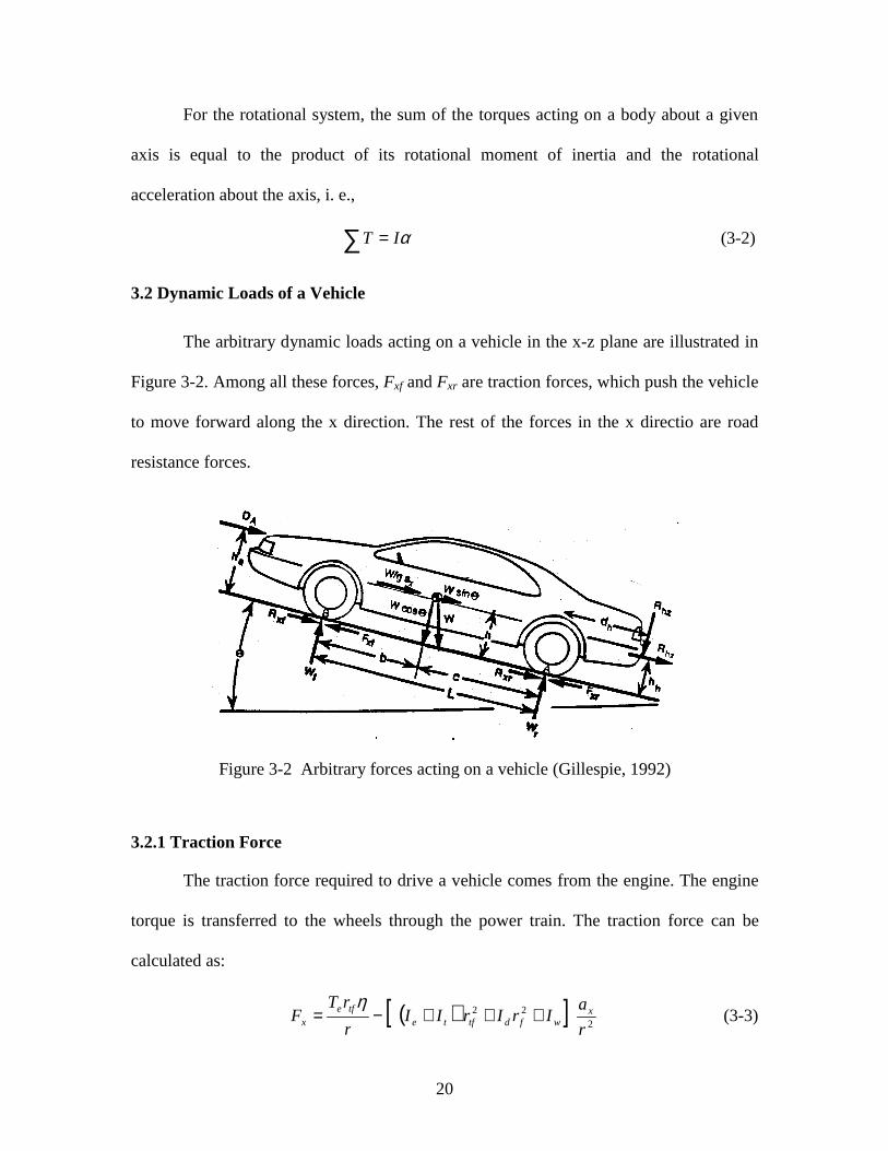
The engine output torque varies with the throttle valve opening and the engine
speed. For a given throttle valve opening, the engine torque varies with the engine speed.
A typical torque surface of a gasoline engine is shown in Figure 3-3.
Figure 3-3 Engine torque as a function of throttling valve opening and engine speed(generated from Fig. 4, Yamaguchi et. al., 1993)
It is noted from this figure that the engine torque is not a linear function of the
engine speed for a given throttle valve opening. For different throttle valve openings the
engine torque exhibits different features. In addition, the throttle valve opening is always
22
changing during the vehicle acceleration period. Therefore, the engine torque can not be
easily defined as some function. If the throttle valve opening is a function of the vehicle
speed determined by the control system, throttle valve opening at any engine speed is
known, thus the engine torque is given.
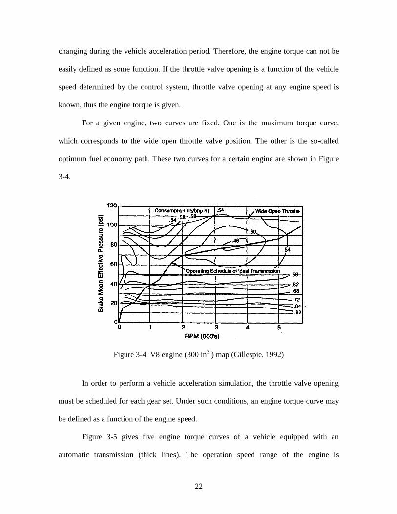
For a given engine, two curves are fixed. One is the maximum torque curve,
which corresponds to the wide open throttle valve position. The other is the so-called
optimum fuel economy path. These two curves for a certain engine are shown in Figure
3-4.
Figure 3-4 V8 engine (300 in3 ) map (Gillespie, 1992)
In order to perform a vehicle acceleration simulation, the throttle valve opening
must be scheduled for each gear set. Under such conditions, an engine torque curve may
be defined as a function of the engine speed.
Figure 3-5 gives five engine torque curves of a vehicle equipped with an
automatic transmission (thick lines). The operation speed range of the engine is
23
1000~3500 rpm. These five curves correspond to five transmission ratios. They are
defined by first scheduling the throttle valve opening. Once such curves are obtained,
acceleration simulation can be completed.
Error! Objects cannot be created from editing field codes.
Figure 3-5 Engine torque as a function of engine speed for five gear sets
Assume that the engine idling speed is ωe0, at which the engine torque is Te0, and
the maximum engine operating speed is ωemax, at which the engine reaches its torque Tef.
To find the vehicle acceleration, the torque curve between Te0 and Tef can be
approximately defined as a quadratic function of the engine speed ωe:
cbaT eee ++= ωω 2 (3-4)
The vehicle speed is directly proportional to the engine speed and dependent on
the gear ratios of the transmission and the final differential drive. The relationship
between the vehicle speed and the engine speed can be expressed as:
Vr
rtfe ⋅=ω (3-5)
Using Eq. (3-5) the engine torque can therefore be expressed as a function of the vehicle
velocity:
)( 2 cqVpVTe ++= (3-6)
where the two coefficients are:
2
=
r
rap tf (3-7)
and
24
r
rbq tf= (3-8)
3.2.2 Aerodynamic Drag
As a result of the air stream interacting with the vehicle, six components of forces
and moments are imposed. These components are drag and rolling moment in the
longitudinal direction, sideforce and pitching moment in the lateral direction, and lift and
yawing moment in the vertical direction. Among them, drag is the largest and most
important aerodynamic force encountered by vehicles at normal highway speeds. It acts
on the vehicle body in the direction of vehicle motion, i.e., x direction. Aerodynamic drag
is a function of vehicle relative velocity, Vr. It can be characterized by the equation:
ACVD DrA2
2
1 ρ= (3-9)
where ρ is the air density, A stands for the frontal area of the vehicle, while CD is called
the drag coefficient.
3.2.2.1 Air Density
The air density is variable depending on temperature, pressure, and humidity
conditions. Under standard conditions (59o F and 29.92 inches Hg or 15o C and 760 mm
of Hg) the density ρ = 0.00236 lb-sec2 /ft4 (1.225 N-sec2/m4). Density under other
conditions can be estimated for the prevailing pressure and temperature conditions by the
equation:
+
⋅=r
r
T
P
460
519
92.2900236.0ρ (3-10)
where:
Pr = Atmospheric pressure in inches of mercury
25
and Tr = Air temperature in degrees Fahrenheit,
or by the equation:
+
⋅=r
r
T
P
16.273
16.288
325.101225.1ρ (3-11)
where:
Pr = Atmospheric pressure in kiloPascale
and Tr = Air temperature in degrees Celsius.
3.2.2.2 Drag Coefficient
The drag coefficient varies over a broad range with different shapes, and should
be determined by wind tunnel tests for each specific vehicle. For a passenger car made in
the late 1980’s, the CD = 0.3 ~ 0.4. For a pick-up truck, the CD may be about 0.45
(Gillespie, 1992).
3.2.2.3 Vehicle Relative Velocity
Velocity used to evaluate aerodynamic drag is the relative velocity of the vehicle
to the wind. This velocity can be expressed as a summation of the vehicle velocity and
the component of wind velocity in the direction of the vehicle travel, i. e.,
Wr VVV += (3-12)
where Vw is the wind speed component in the direction of vehicle travel. When the wind
blows toward the vehicle a headwind is present. Wind blowing in the direction of vehicle
travel is a tailwind. For headwind, Vw is positive, while for tailwind Vw is negative.
Bringing Eq. (3-12) into Eq. (3-9), the drag can be defined as:
)2(2
1 22WWDA VVVVACD ++= ρ (3-13)
26
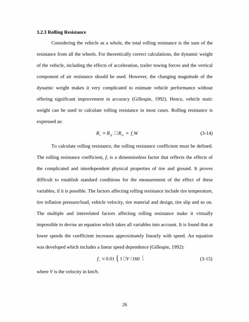
3.2.3 Rolling Resistance
Considering the vehicle as a whole, the total rolling resistance is the sum of the
resistance from all the wheels. For theoretically correct calculations, the dynamic weight
of the vehicle, including the effects of acceleration, trailer towing forces and the vertical
component of air resistance should be used. However, the changing magnitude of the
dynamic weight makes it very complicated to estimate vehicle performance without
offering significant improvement in accuracy (Gillespie, 1992). Hence, vehicle static
weight can be used to calculate rolling resistance in most cases. Rolling resistance is
expressed as:
WfRRR rxrxfx =+= (3-14)
To calculate rolling resistance, the rolling resistance coefficient must be defined.
The rolling resistance coefficient, fr is a dimensionless factor that reflects the effects of
the complicated and interdependent physical properties of tire and ground. It proves
difficult to establish standard conditions for the measurement of the effect of these
variables, if it is possible. The factors affecting rolling resistance include tire temperature,
tire inflation pressure/load, vehicle velocity, tire material and design, tire slip and so on.
The multiple and interrelated factors affecting rolling resistance make it virtually
impossible to devise an equation which takes all variables into account. It is found that at
lower speeds the coefficient increases approximately linearly with speed. An equation
was developed which includes a linear speed dependence (Gillespie, 1992):
( )160/101.0 Vfr += (3-15)
where V is the velocity in km/h.
27
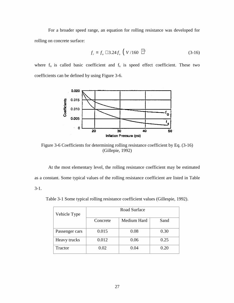
For a broader speed range, an equation for rolling resistance was developed for
rolling on concrete surface:
( ) 5.2160/24.3 Vfff sor += (3-16)
where fo is called basic coefficient and fs is speed effect coefficient. These two
coefficients can be defined by using Figure 3-6.
Figure 3-6 Coefficients for determining rolling resistance coefficient by Eq. (3-16)(Gillepie, 1992)
At the most elementary level, the rolling resistance coefficient may be estimated
as a constant. Some typical values of the rolling resistance coefficient are listed in Table
3-1.
Table 3-1 Some typical rolling resistance coefficient values (Gillespie, 1992).
Road SurfaceVehicle Type
Concrete Medium Hard Sand
Passenger cars 0.015 0.08 0.30
Heavy trucks 0.012 0.06 0.25
Tractor 0.02 0.04 0.20
28
3.3 Vehicle Acceleration
Knowing the traction force and each term of the road load, it is possible to predict
the acceleration performance of the vehicle. By using the Second Law, the equation takes
the form:
θsinWRDRFMa hxAxxx −−−−= (3-17)
Equation.(3-3) shows that the traction force term includes the engine torque and
rotational inertia terms. The rotational inertias are often lumped in with the mass of the
vehicle to obtain a simplified equation:
θη
sin)( WRDRr
rTaMM hxAx
tfexr −−−−=+ (3-18)
where Mr is called the equivalent mass of the rotating components. The combination of
the two masses is then called an effective mass. Let
M
MMk r+
= (3-19)
be the mass factor. The mass factor will depend on the operating gear. A representative
number is often taken as (Gillespie, 1992):
20025.004.01 tfrk ++= (3-20)
Using the mass factor k, Eq. (3-18) can be rewritten as
θη
sinWRDRr
rTkMa hxAx
tfex −−−−= (3-21)
The right-hand side of Eq. (3-21) involves the vehicle velocity (first and second
order), while the left-hand side involves vehicle’s acceleration, which is the first
derivative of velocity to time. When CVPST is used, both rtf and η are functions of the
29
velocity. Hence a general differential equation is encountered to solve for vehicle
acceleration performance. This equation can be expressed as follows:
0)()()( 2’ =+++ tCVtBVtAV (3-22)
Functions A(t), B(t), and C(t) depend on the torque curve, the rolling resistance
equation, and the transmission selection. For a standard transmission, the total ratio and
efficiency are fixed values at each gear set; while for a CVPST, they vary with the
velocity (or time). These functions will be defined in Chapter 5.
30
CHAPTER 4 CONTINUOUSLY VARIABLE POWER SPLIT TRANSMISSION
(CVPST) ANALYSIS
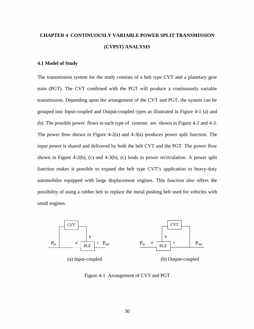
4.1 Model of Study
The transmission system for the study consists of a belt type CVT and a planetary gear
train (PGT). The CVT combined with the PGT will produce a continuously variable
transmission. Depending upon the arrangement of the CVT and PGT, the system can be
grouped into Input-coupled and Output-coupled types as illustrated in Figure 4-1 (a) and
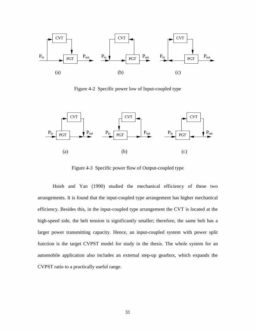
(b). The possible power flows in each type of systems are shown in Figure 4-2 and 4-3.
The power flow shown in Figure 4-2(a) and 4-3(a) produces power split function. The
input power is shared and delivered by both the belt CVT and the PGT. The power flow
shown in Figure 4-2(b), (c) and 4-3(b), (c) leads to power recirculation. A power split
function makes it possible to expand the belt type CVT’s application to heavy-duty
automobiles equipped with large displacement engines. This function also offers the
possibility of using a rubber belt to replace the metal pushing belt used for vehicles with
small engines.
CVT
PGTa
bcPin Pout
CVT
PGTa
b
cPin Pout
(a) Input-coupled (b) Output-coupled
Figure 4-1 Arrangement of CVT and PGT
31
CVT
PGTPin Pout
CVT
PGTPin Pout
CVT
PGTPin Pout
(a) (b) (c)
Figure 4-2 Specific power low of Input-coupled type
CVT
PGTPin Pout
CVT
PGTPin Pout
CVT
PGTPin Pout
(a) (b) (c)
Figure 4-3 Specific power flow of Output-coupled type
Hsieh and Yan (1990) studied the mechanical efficiency of these two
arrangements. It is found that the input-coupled type arrangement has higher mechanical
efficiency. Besides this, in the input-coupled type arrangement the CVT is located at the
high-speed side, the belt tension is significantly smaller; therefore, the same belt has a
larger power transmitting capacity. Hence, an input-coupled system with power split
function is the target CVPST model for study in the thesis. The whole system for an
automobile application also includes an external step-up gearbox, which expands the
CVPST ratio to a practically useful range.
32
4.2 System Analysis
4.2.1 CVPST Ratio
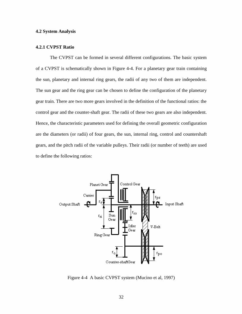
The CVPST can be formed in several different configurations. The basic system
of a CVPST is schematically shown in Figure 4-4. For a planetary gear train containing
the sun, planetary and internal ring gears, the radii of any two of them are independent.
The sun gear and the ring gear can be chosen to define the configuration of the planetary
gear train. There are two more gears involved in the definition of the functional ratios: the
control gear and the counter-shaft gear. The radii of these two gears are also independent.
Hence, the characteristic parameters used for defining the overall geometric configuration
are the diameters (or radii) of four gears, the sun, internal ring, control and countershaft
gears, and the pitch radii of the variable pulleys. Their radii (or number of teeth) are used
to define the following ratios:
Figure 4-4 A basic CVPST system (Mucino et al, 1997)
33
,ri
sg r
rr = ,
ro
ocg r
rr = and
ps
poc r
rr = (4-1)
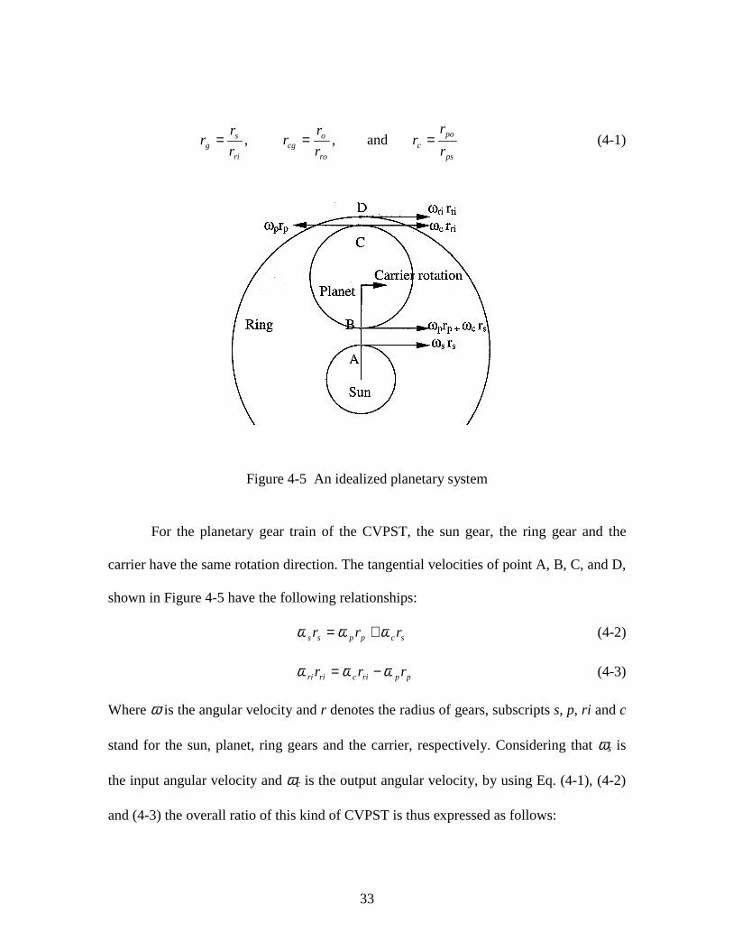
Figure 4-5 An idealized planetary system
For the planetary gear train of the CVPST, the sun gear, the ring gear and the
carrier have the same rotation direction. The tangential velocities of point A, B, C, and D,
shown in Figure 4-5 have the following relationships:
scppss rrr ωωω += (4-2)
ppricriri rrr ωωω −= (4-3)
Where ω is the angular velocity and r denotes the radius of gears, subscripts s, p, ri and c
stand for the sun, planet, ring gears and the carrier, respectively. Considering that ωs is
the input angular velocity and ωc is the output angular velocity, by using Eq. (4-1), (4-2)
and (4-3) the overall ratio of this kind of CVPST is thus expressed as follows:
34
cggc
gc
out
int rrr
rrr
++
==)1(
ωω
(4-4)
4.2.2 Power Split Factor
The key factor in distinguishing a power split system and a power recirculation
system is the circulating power ratio. If Pcir is used to stand for the circulating power and
Pc for the output power, the circulating power ratio is:
c
cir
P
P=γ (4-5)
If the input angular velocity of a differential planetary gear train is denoted as ωa, the
output angular velocity is ωc and the angular velocity of the element connected to the
control unit is ωb (see Figure 4-1a), then the circulating power ratio is (Mabie and
Reinholtz, 1987):
)(
)(
bac
acb
ωωωωωωγ
−−
= (4-6)
or
’1
)1(’
r
Rr
−−=γ (4-7)
where a
brωω
=’ and c
aRωω
= .
The circulating power ratio, γ, is a key factor. If γ is positive, it means that there is
power recirculating in the system. If γ is negative, a power split system is formed.
For the configuration of the CVPST shown in Figure 4-4, ina ωω = , outc ωω = ,
rib ωω = . Because the ring gear and the control gear have the same angular velocity and
it can be expressed in terms of input speed:
35
c
cginri r
rωω =
this gives:
c
cg
r
rr =’
Since R is the CVPST ratio given in Eq. (4-4), hence, for the configuration shown in
Figure 4-4, it gives:
cggc
cg
rrr
r
+−=γ (4-8)
It is obvious that this configuration is really a power split system because γ is always
negative.
4.2.3 Power Flow
The input power of the CVPST is split into two parts flowing through the gear
and the CVT belt, respectively. The amount of power flowing through the gear and the
CVT depends upon the ratios defined by Eq. (4-1). If neglecting the mechanical
efficiency of the transmission, the output power is equal to the input power. The power
flowing through the CVT is thus expressed as:
cggc
cg
in
CVT
rrr
r
P
P
+= (4-9)
The torque going into the sun gear and the CVT belt can be expressed by the
following equations (Mucino et al., 1997):
cggc
gc
in
PGT
rrr
rr
T
T
+= (4-10)
36
cggc
cg
in
CVT
rrr
r
T
T
+= (4-11)
g
g
PGT
out
r
r
T
T 1+= (4-12)
cg
gc
CVT
out
r
rr
T
T )1( += (4-13)
cg
gc
CVT
PGT
r
rr
T
T= (4-14)
By using these equations, the power flowing through the PGT and the CVT can be
calculated as follows:
incggc
cgininCVTCVT rrr
rTTP ωω
+== (4-15)
incggc
gcininPGTPGT rrr
rrTTP ωω
+== (4-16)
Since the tension in the CVT belt is
cggc
cg
ps
in
ps
CVTbelt rrr
r
r
T
r
TF
+== (4-17)
then the power through the CVT and the PGT can be expressed in terms of the belt
tension:
inpsbeltCVT rFP ω= (4-18)
)( psbeltininPGT rFTP −= ω (4-19)
For the CVPST it is desirable that at low speeds (rc = rcmax) the power flowing
through the belt be less than that flowing through the PGT, but at high speeds (rc = rcmin)
37
the power flowing through the belt should be greater than that flowing through the PGT.
These two situations are denoted by 1≥CVT
PGT
T
T and 1≤
CVT
PGT
T
T. From Eq. (4-14) these can
be rewritten as rcg ≤ rgrcmax and rcg ≥ rg rcmin. Hence, there must exist an intermediate
value of rc = rcm in which case rcg = rcm rg thus 1=CVT
PGT
T
T, where rcm is defined by the
following equation:
minminmax0 )( ccccm rrrcr +−= (4-20)
where c0 is introduced as the crossover coefficient which has the value between 0 and 1
and designates where the power crossover is to occur. Once the crossover coefficient is
given, the ratio of rg and rcg is fixed. Hence, one design degree of freedom is eliminated
by defining the crossover coefficient.
4.3 CVPST System Design
4.3.1 Determination of rg and rcg
A CVPST geometric configuration is determined by three ratios defined by Eq.
(4-1). For an actual application of CVPST a total ratio span is assumed to be given and is
denoted with rtmax and rtmin. If a standard belt CVT is used, a certain variator ratio span is
also fixed as rcmax and rcmin. Using Eq.(4-2) and considering that rc = rcmax when rt = rtmax
and rc = rcmin when rt = rtmin, the following two equations are obtained:
cggc
gct rrr
rrr
++
=max
maxmax
)1( (4-21)
and
38
cggc
gct rrr
rrr
++
=min
minmin
)1( (4-22)
From these two equations the gear ratios rg and rcg are expressed in terms of maximum
and minimum transmission and in terms of the maximum and minimum variator ratio.
The solutions for rg and rcg are (Mucino et. al., 1997):
)1()1( maxmaxminminminmax
minmaxminmax
−−−−
=tcttct
tcctg rrrrrr
rrrrr (4-23)
)1()1(
)(
minminmaxmaxmaxmin
minmaxminmax
−−−−
=tcttct
ttcccg rrrrrr
rrrrr (4-24)
Eq. (4-23) and (4-24) are used to determine rg and rcg by the high and low values
of the transmission and variator ratios. Knowing these two ratios, the crossover
coefficient c0 can be found.
If the crossover coefficient is first given, rg and rcg no longer are independent of
each other. In this case, Eq. (4-20) is used to find rcm which denotes the ratio of rcg to rg;
then either the maximum transmission ratio or the minimum transmission ratio is fixed,
while the other is found by solving Eq. (4-23) and (4-24) simultaneously. Assuming that
the maximum transmission ratio is fixed, the minimum transmission ratio is found by:
maxmin
max
max
minmin t
ccm
ccm
c
ct r
rr
rr
r
rr
++
= (4-25)
Once rcmin is found, Eq. (4-23) and (4-24) are used to find the values of rg and rcg.
The ratio values of rg and rcg may be further limited by the belt torque capacity.
Assume that the belt power capacity is known. If the total input torque is given, the
torque transferred by the PGT is also known as TPGT = Tin - TCVT. In this case, the ratio of
rcg to rg is also a fixed value which is given by:
39
PGT
CVTc
g
cg
T
Tr
r
r= (4-26)
Then similar steps are executed to find rtmin and then rg and rcg.
4.3.2 Step-up Gear Ratio
It is possible to produce a continuously variable transmission with a wide span of
overall ratios by using a step-up gearbox to expand the limited CVPST ratio span for the
automotive application. This enables the variator ratio to be chosen within a narrow range
in which the CVT has the maximum mechanical efficiency which improves the total
efficiency of the transmission. For the design of a CVPST system, the step-up gear ratio,
rst, needs to be determined.
It is assumed that the overall ratio of the transmission, including the CVPST and
the step-up gear is denoted as rto. This ratio can be expressed as:
sttto rrr = (4-27)
For a given CVPST ratio span, the overall ratio is obtained by setting the step-up gear
ratio. The step-up gear ratio is thus calculated by:
t
tost r
rr = (4-28)
When the vehicle starts acceleration at low speeds, the required torque is large. To
provide the vehicle enough traction force for acceleration and to split the most power
flowing through the PGT, the maximum total ratio is required and the maximum CVPST
ratio is used. In this case, the step-up gear ratio, denoted as rst1, is:
max
max1
t
tost r
rr = (4-29)
40
When the variator ratio decreases to its minimum value during the vehicle acceleration,
which means the CVPST ratio also reaches its minimum value, a shift occurs. The first
step-up gear set is separated and the second step-up gear set is meshed. To maintain a
continuous ratio, the second step-up gear ratio must satisfy the following relationship:
max
min12
t
tstst r
rrr ≥ (4-30)
Eq. (4-30) gives a lower bond for the second step-up gear ratio. When the vehicle reaches
the target velocity and starts to cruise at that velocity, an ideal state is that the variator
ratio becomes 1, which gives maximum transmission efficiency. In this case, the step-up
gear ratio should satisfy the following relationship:
thf
est rrV
rr
max
max2 6.3
ω=
where rth stands for the ratio of the CVPST with the maximum efficiency. If choosing
variator ratio to be 1, rth can be found as:
cgg
gth rr
rr
++
=1
Hence, the second step-up gear ratio is:
g
cgg
f
est r
rr
rV
rr
++
=1
6.3max
max2
ω(4-31)
Eq.(4-31) gives an upper bound for the step-up gear ratio. If overdrive is required, the
step-up gear ratio should be found by the given minimum total ratio:
th
tost r
rr min
2= (4-32)
41
From the analysis above, at least two step-up gear sets are necessary to construct a
continuous ratio span and to accomplish the vehicle acceleration and the change from the
acceleration to the cruise travel.
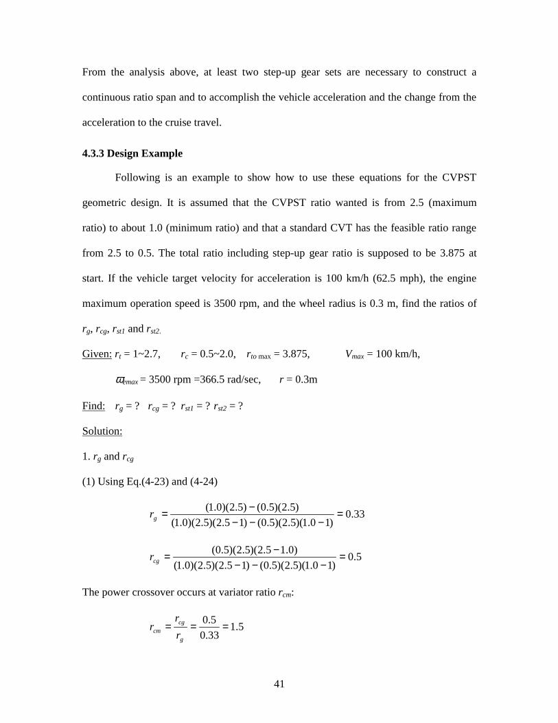
4.3.3 Design Example
Following is an example to show how to use these equations for the CVPST
geometric design. It is assumed that the CVPST ratio wanted is from 2.5 (maximum
ratio) to about 1.0 (minimum ratio) and that a standard CVT has the feasible ratio range
from 2.5 to 0.5. The total ratio including step-up gear ratio is supposed to be 3.875 at
start. If the vehicle target velocity for acceleration is 100 km/h (62.5 mph), the engine
maximum operation speed is 3500 rpm, and the wheel radius is 0.3 m, find the ratios of
rg, rcg, rst1 and rst2.
Given: rt = 1~2.7, rc = 0.5~2.0, rto max = 3.875, Vmax = 100 km/h,
ωemax = 3500 rpm =366.5 rad/sec, r = 0.3m
Find: rg = ? rcg = ? rst1 = ? rst2 = ?
Solution:
1. rg and rcg
(1) Using Eq.(4-23) and (4-24)
33.0)10.1)(5.2)(5.0()15.2)(5.2)(0.1(
)5.2)(5.0()5.2)(0.1( =−−−
−=gr
5.0)10.1)(5.2)(5.0()15.2)(5.2)(0.1(
)0.15.2)(5.2)(5.0( =−−−
−=cgr
The power crossover occurs at variator ratio rcm:
5.133.0
5.0 ===g
cgcm r
rr
42
The corresponding crossover coefficient is:
5.05.05.2
5.05.1
minmax
min0 =
−−=
−−
=cc
ccm
rr
rrc
(2) Setting the crossover coefficient c0 = 0.75, which leads to the power crossover to
occur closer to the low pulley ratio, and using Eq. (4-20)
rcm = (0.75)(2.5-0.5) + 0.5 = 2
then using Eq. (4-22)
9.05.25.02
5.22
5.2
5.0min =
++=tr
Now rg and rcg can be found by using Eq. (4-23) and (4-24). They are:
286.0)19.0)(5.2)(5.0()15.2)(5.2)(9.0(
)5.2)(5.0()5.2)(9.0( =−−−
−=gr
572.0)19.0)(5.2)(5.0()15.2)(5.2)(9.0(
)9.05.2)(5.2)(5.0( =−−−
−=cgr
(3) If the belt torque limit is 40% of the input torque at the low speed with rc = 2.5, then
using Eq. (4-26), (4-25), (4-23) and (4-24), rg and rcg can be found by the following steps:
67.14.01
4.05.2 =
−===
PGT
CVTc
g
cgcm T
Tr
r
rr
96.05.25.067.1
5.267.1
5.2
5.0min =
++=tr
315.0)196.0)(5.2)(5.0()15.2)(5.2)(96.0(
)5.2)(5.0()5.2)(96.0( =−−−
−=gr
527.0)196.0)(5.2)(5.0()15.2)(5.2)(96.0(
)96.05.2)(5.2)(5.0( =−−−
−=cgr
2. Step-up Gear ratios
Using Eq. (4-29), the first step-up gear ratio is found as:
43
55.1)5.2)(0.4(
5.151 ==str
If rg = 0.28 and rcg = 0.57 then rth = rt = 1.5 when rc = 1.0, therefore
66.0)5.1)(0.4)(100(
)3.0)(5.366(6.32 ==str
Since 395.1)9.0)(55.1(min1 ==tst rr < max2)5.2)(66.0(65.1 tst rr== , a continuous
ratio is obtained.
If overdrive is required and the minimum total transmission ratio is 0.694, then
the second step-up gear ratio should be:
46.05.1
694.02 ==str
Since 15.1)5.2)(46.0(max2 ==tst rr < 1.395, in order to obtain a continuous ratio,
some modification is required. Assuming that the minimum CVPST ratio is changeable,
the new rtmin is found by setting the two sides of Eq. (4-32) to be equal. This gives:
74.055.1
)5.2)(46.0(
1
max2min ===
st
tstt r
rrr
By using the new rtmin, rg and rcg can be found. They are rg = 0.19 and rcg = 0.71.
The corresponding power flowing through the belt is 60 percent of the input power. The
belt capacity should be checked after this modification.
The step-up gear ratio selection above enables the vehicle to have a continuously
variable transmission ratio span of 3.875~0.694.
44
CHAPTER 5 SIMULATION EQUATIONS OF VEHICLE ACCELERATION
Vehicle drive test and simulation involves the solution of the differential equation
(3-22). The solution of this equation depends upon certain conditions. For vehicles
equipped with a CVPST at low speeds, and for vehicles with standard transmissions or
automatic transmissions neglecting the change in torque converter efficiency, the total
ratio and efficiency for each gear set are constant. The engine speed may experience
high-low-high variations during the acceleration period. For vehicles with CVPST at
higher speeds, both the total ratio and efficiency are velocity (or time) dependent, while
the engine can operate at a constant speed. Hence, the solution for Eq. (3-22) is different.
Since vehicles with CVPST may encounter a fixed ratio and thus a fixed efficiency at low
speeds, in this chapter Eq. (3-22) is first solved by considering both the total ratio and
efficiency as constant. Then simulation equations for the CVPST are derived based on
some assumptions. The solution obtained in this chapter can also be used for the
simulation of vehicles equipped with step-ratio transmissions.
5.1 Simulation Equations for Constant Transmission Ratio and Efficiency
5.1.1 Equation Simplification
Using Eq. (3-6), (3-13), and (3-16), Eq. (3-22) may take the following form:
( )( ) WVffcqVpVr
rkMa so
tfx
5.22 160/24.3)( +−++=η
(5-1)
θρ sin)2(2
1 22 WRVVVVAC hxwwD −−++−
Obviously it is very difficult to find a theoretical solution for Eq. (5-1). If the
rolling resistance coefficient is defined as a linear function of the vehicle velocity, as
45
using Eq. (3-15), for a fixed gear ratio and mechanical efficiency, Eq. (5-1) may take the
following form:
CQVPVdt
dV ++= 2 (5-2)
where P, Q, and C are constant for each gear set. Eq. (5-2) is variable-separable, thus, a
theoretical solution is available for a given set of values of P, Q, and C. Unfortunately,
what kind of form the solution will take depends upon the values of P, Q, and C. There is
not a unique solution function. For example, if the right-hand side of Eq. (5-2) is
442 ++ VV , the solution involves 1/t; If it is 22 ++ VV , the solution is related to tan(t);
while 232 ++ VV may lead the solution to take the form of an exponential expression.
The uncertain solution of the function makes it very difficult to program if it is even
possible. To solve this equation for vehicle velocity and acceleration as functions of time,
Eq. (5-1) must be simplified based on some reasonable conditions.
5.1.1.1 Engine Torque
From the description in Chapter 3, the output torque of an engine is a function of
the engine speed and the throttle valve opening. For a vehicle equipped with a standard
transmission, the throttle valve opening is directly controlled by the driver. Different
drivers will produce different vehicle performance. For a vehicle equipped with an
automatic transmission, it might now be controlled by an electronic control system. This
allows the driver to select a preferred shift schedule mode by means of a control switch
operation. The common thing for such multi-ratio transmissions is that the engine speed
keeps varying in the vehicle acceleration process due to shifting. Different shift schedules
will produce different engine operating paths, thus producing different vehicle velocity
46
and acceleration characteristics. To simulate the vehicle acceleration performance, the
first step is to define the engine torque function.
For a given engine map, the engine torque can be defined as a function of vehicle
speed as described with Eq. (3-6) in Chapter 3. To avoid the second order term, the
quadratic torque curve is represented with several straight lines described as follows:
cqVTe += (5-3)
Each straight line is applied to Eq. (3-6) as the traction force term. For different gear
ratios and segments of torque curve, q and c should be calculated by using different rtf
values and torque curve parameters.
5.1.1.2 Rolling Resistance
The rolling resistance coefficient, as mentioned in Chapter 3, can be evaluated by
Eq. (3-15) or (3-16). Assume that the vehicle is accelerated from V = 0 to V = 120 km/h
(75 mph). If using Eq. (3-15):
( )=+= 160/)120~0(101.0rf 0.01 to 0.0175
If using Eq.(3-16) and considering 30 psi inflation pressure which corresponds to fo =
0.01 and fs = 0.005 from Figure 3-6, then
( ) =+= 5.2)160/)120~0(*005.0*24.301.0rf 0.01 to 0.0179
It is obvious that there is little difference between the results obtained by using
these two equations. Linear Eq. (3-15) simplifies the rolling resistance term and has little
effect on accuracy.
5.1.1.3 Drag Term
Drag term is related to the relative velocity of the vehicle. The wind speed is
assumed to be a constant for the simulation. Hence, the drag will vary with the vehicle
47
velocity. Theoretically, the drag term should be combined with the traction force term. If
the time interval of the simulation is small enough, the velocity change from step to step
is not large. It is therefore possible to use an estimated velocity to evaluate the drag. To
minimize the error, the vehicle velocity at the last simulation step plus the velocity
difference of the last two steps is used as the estimated vehicle velocity. This enables the
drag to be treated as a constant term at each step. In such a way the accuracy is sufficient.
5.1.2 Solution of the Equation for Constant Ratio and Efficiency
By representing the torque curve with several linear functions, using the linear
equation for rolling resistance, and treating drag as a constant term, Eq. (5-1) becomes:
hxWeDtf RVVACWVcqVr
r
dt
dVkM −+−++−+= 2)(
2
1)sin)160/1(01.0()( ρθ
η (5-4)
Eq. (5-4) can be simply expressed as
CQVdt
dV += (5-5)
where the coefficients Q and C are:
)16000
(1 Mg
qr
r
kMQ tf −=
η (5-6)
−+−+−= hxWeD
tf RVVACWcr
r
kMC 2)(
2
1)sin01.0(
1 ρθη
(5-7)
Ve is the estimated velocity. When t = 0 Ve = 0; when t = 0.1 second (simulation time
interval), Ve is assumed to be 0.1.
The vehicle velocity as a function of the acceleration time can be found by
solving Eq. (5-5). It gives:
−
+= −
Q
Ce
Q
QVCV ttQ )(0 0
6.3/6.3 (km/h) (5-8)
48
The vehicle acceleration and displacement, as functions of the acceleration time, can then
be obtained by finding the first derivative of Eq. (5-8) to time and integrating Eq. (5-8) to
time, respectively. They are:
)(0
0)6.3/( ttQx eQVCa −+= (m/s2) (5-9)
00)(
20 )()1(
6.3/0 Dtt
Q
Ce
Q
QVCD ttQ +−−−
+= − (m) (5-10)
Eq. (5-8), (5-9) and (5-10) can be used for the simulation of vehicles equipped
with standard and automatic transmissions, as well as the CVPST when the transmission
ratio is a constant value at low vehicle speeds.
5.2 Simulation Equations for Variable Transmission Ratio and Efficiency
Vehicles equipped with CVPST present a different acceleration performance. Due
to the stepless ratio change, it is possible for the engine to work at the optimum point at
which it reaches its maximum efficiency (Guo et. al., 1988). For the acceleration
simulation of a vehicle with CVPST combined with a step-up gearbox, it is assumed that
the vehicle acceleration from the static state to a target velocity involves three stages. In
the first stage, the vehicle starts to accelerate with the engine speed increasing from the
idling speed to the maximum operation speed. After the engine reaches the maximum
operation speed, it is possible to stay at that speed, while the transmission ratio will
decrease with the increase in vehicle velocity. At the first stage, a large total ratio is
necessary to ensure that the vehicle gains sufficient traction force for acceleration. The
49
CVPST should also distribute the majority of power flowing through the gear. From the
analysis described in Chapter 4, a higher variator ratio will lead to a higher CVPST ratio.
A high CVPST ratio combined with a step-up gear ratio should produce a large
transmission ratio. This matches the large ratio requirement. From Eq. (4-15) it is noted
that the power flowing through the belt decreases with the increase in the variator ratio.
Hence, to use as high a variator ratio as possible also matches the requirement of
reducing the power flowing through the belt at low speeds. It is therefore a smart choice
for the CVPST ratio to be fixed at a high value at the low speed stage. Once the engine
reaches its maximum operating speed, the first stage is over. In the second stage, the
CVPST ratio starts decreasing with the increase in the vehicle velocity. When the CVPST
ratio is decreased to its minimum value (or some designed value), the first step-up gear is
separated and the second step-up gear starts to mesh. The second stage is completed and
the third stage begins. The CVPST ratio should then be adjusted to a certain value to keep
the total transmission ratio the same as before switching. For example, if the total
transmission ratio is 3.875~0.72 and CVPST ratio is 2.7~0.9, two step-up gear ratios are
1.435 and 0.48, and step-up gear switch occurs at the CVPST ratio of 0.9; the CVPST
ratio should be adjusted back to 2.7. In the third stage, the CVPST ratio keeps decreasing
until the vehicle reaches the target velocity. The optimum condition is that the variator
ratio of the CVPST is back to 1 when the vehicle is accelerated to the target velocity,
because this enables the vehicle to cruise at that speed with the maximum transmission
and engine efficiency.
50
5.2.1 Shift Velocity
It is assumed that the vehicle is accelerated from a static state to a certain velocity.
At stage I, the engine speed increases from the idle speed to the maximum operating
speed. Vehicle velocity increases with the increase in engine speed. The CVPST takes the
maximum ratio and the first step-up gear set is meshed. The first shift velocity , V1, is
found by:
max1
max1 6.3
tstf
e
rrr
rV
ω= (5-11)
At stage II, the CVPST ratio continuously decreases from its maximum value to the
minimum value. The first step-up gear is still in use. The vehicle velocity increases with
the decrease in the CVPST ratio. The second shift velocity is easily found by the
following equation:
min1
max2 6.3
tstf
e
rrr
rV
ω= (5-12)
At stage III, the second step-up gear is meshed and the CVPST ratio goes back to
some value (corresponding to the total ratio at the end of stage II), then again decreases
continuously. This value can be calculated as:
2
1min
st
sttt r
rrr = (5-13)
When the vehicle velocity reaches the target velocity, the CVPST ratio will be
adjusted to rth which corresponds to the variator ratio of 1, the engine speed is:
r
rrrV stthfe 6.3
2max=ω (5-14)
51
5.2.2 Equations for Simulation
The vehicle acceleration at stage I is the same as that of a vehicle equipped with a
standard transmission. At this stage the vehicle velocity, acceleration, and displacement
can be calculated with Eq. (5-8), (5-9) and (5-10).
Different from the first stage, at stage II and III the engine keeps working at its
maximum speed with a constant throttle opening, while the transmission ratio varies with
a decrease in the variator ratio. Therefore, the input torque will remain a constant value,
but the traction force will be a function of the transmission ratio and efficiency, which is
also a function of the transmission ratio.
5.2.2.1 Transmission Ratio
At stage II and III, the transmission ratio varies with the change of variator ratio rc
during the vehicle acceleration. At any acceleration time t, the transmission ratio
(including the step-up gear ratio) has to obey the following relationship:
Vr
rr
f
eto
maxω= (5-15)
where
sttto rrr = (5-16)
5.2.2.2 CVPST Efficiency
As described before, the CVT efficiency is a function of the variator ratio. The
power loss of a CVPST as a function of the variator ratio is shown in Figure 5-1. This
figure shows that the maximum efficiency is obtained at rc = 1. Different arrangements of
CVPST may produce different power loss curves, however, in most cases, the power loss
curves of the CVPST have similar configurations. From this power loss curve, the
CVPST efficiency as a function of the variator ratio can be found as shown in Figure 5-2.
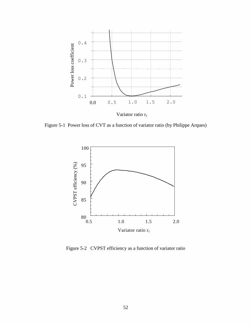
52
0.5 1.0 1.5 2.0
Pow
er lo
ss c
oeff
icie
nt
0.1
0.2
0.3
Variator ratio rc
0.4
0.0
Figure 5-1 Power loss of CVT as a function of variator ratio (by Philippe Arques)
0.5 1.5 2.01.0
Variator ratio rc
80
85
90
95
100
CV
PST
eff
icie
ncy
(%)
Figure 5-2 CVPST efficiency as a function of variator ratio
53
The overall efficiency of the CVPST also reaches its maximum value at the
variator ratio of 1.0. This CVPST efficiency curve can be best fitted by two quadratic
functions. They are:
47.5984.69091.36 2 ++−= cct rrη ( 0.5 ≤ rc ≤ 1.0 )
and
54.899364.72592.4 2 ++−= cct rrη ( 1.0 ≤ rc ≤ 2.0 )
These two equations can be rewritten in a generic form as follows:
usrnr cct ++= 2η (5-17)
5.2.3 Differential Equation and Solutions
At the second and the third stages, there are two choices to evaluate the rolling
resistance force. One is to calculate the rolling resistance force using the velocity
obtained from the last step; the other is using a constant value for fr. The drag is
calculated with the same method as used in the standard transmission simulation. The
mass factor, k, is considered a constant since the total inertia is almost the same at these
stages, though the variator ratio changes. Mechanical efficiency is evaluated using the
current variator ratio before each simulation step. It can be treated as a constant for each
step. The differential equation for these two stages becomes:
hxrADtofe
x RWfFrr
rTkMa −+−−= )sin(max θ
η (5-18)
Considering that the overall transmission ratio, rto, is a function of the vehicle velocity as
defined with Eq. (5-15), the first term of the right-hand side of Eq. (5-18) can be
rewritten as:
54
V
T ee ηω maxmax
Eq.(5-18) is simply written as follows:
PV
Qax += (5-19)
or
PV
Q
dt
dV += (5-20)
where
kM
TQ ee ηω maxmax= (5-21)
( )hxrAD RWfFkM
P +++−= )sin(1 θ (5-22)
and FAD is the drag and is calculated with Eq. (3-9).
By separating variables and considering the initial condition V = V0 at t = t0, Eq.
(5-20) is solved as
00
20 ln)(1
tPVQ
PVQ
P
QVV
Pt +
++−−= (5-23)
The acceleration time required for a specific target vehicle velocity is easily found by
using this equation. The vehicle acceleration at any simulation step is directly calculated
from the vehicle velocity using Eq. (5-19).
If neglecting the road resistance force term, Eq. (5-21) becomes:
V
Q
dt
dV = (5-24)
The solution of this equation gives the Power-Limited Acceleration performance of a
vehicle. The vehicle velocity, acceleration, and displacement at this state are defined by
following equations:
55
200 )(2 VttQV +−= (5-25)
200 )(2 VttQ
Qax
+−= (5-26)
( ) 03
02
0023
)(23
1DVVttQ
QD +
−+−= (5-27)
56
CHAPTER 6 ACCELERATION SIMULATION RESULTS AND ANALYSIS
A computer program developed in this thesis work simulates the acceleration
performance of vehicles equipped with CVPST. This program also can simulate the
acceleration performance of vehicles equipped with multi-ratio transmissions (standard or
automatic). Another task for this program is to choose the appropriate parameters for
CVPST based on the given engine characteristics and vehicle information. The program
language used is Microsoft Visual Basic 5.0. This software can provide a user-friendly
interface which is suitable when many inputs need to be typed in. It is also very easy to
produce the corresponding graphs using the data generated by the program itself. The
program consists of three main parts, which are the CVPST system design, the
acceleration simulation of vehicle equipped with the CVPST and the multi-ratio
transmission. Program code of these three parts are given in Appendix A. The program is
available to simulate as many as five speed standard or automatic transmissions. The
CVPST system design is completed according to the given belt torque capacity or
transmitted torque requirement.
6.1 Simulation Conditions
6.1.1 Simulation Model
Figure 6-1 shows a block diagram of a vehicle equipped with a typical gasoline
engine and a standard transmission or an automatic transmission. The difference between
these two is that for the standard transmission a clutch is used, while for the automatic
transmission a torque converter is mounted. Figure 6-2 illustrates a block diagram of a
vehicle equipped with a CVPST plus a step-up gearbox. Since at low speed the variator

57
ratio is supposed to be a fixed value, the CVPST with a step-up gearbox is similar to a 2-
speed standard transmission.
Figure 6-1 Simulation model of vehicle with standard or automatic transmission
Figure 6-2 Simulation model of a CVPST with a step-up gearbox
Wheel
Clutch or Torque Converter
Wheel
Diff. Transmission Engine
Wheel
Wheel
Diff.CVPST EngineStep-up
Gearbox
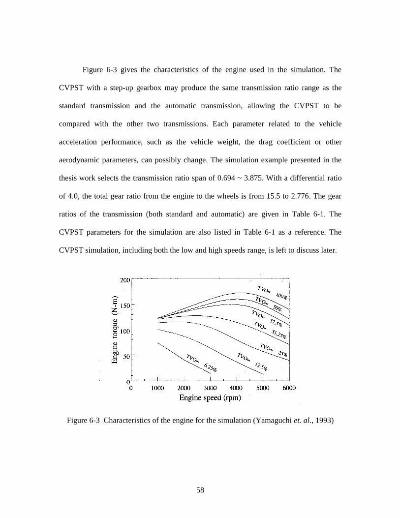
58
Figure 6-3 gives the characteristics of the engine used in the simulation. The
CVPST with a step-up gearbox may produce the same transmission ratio range as the
standard transmission and the automatic transmission, allowing the CVPST to be
compared with the other two transmissions. Each parameter related to the vehicle
acceleration performance, such as the vehicle weight, the drag coefficient or other
aerodynamic parameters, can possibly change. The simulation example presented in the
thesis work selects the transmission ratio span of 0.694 ~ 3.875. With a differential ratio
of 4.0, the total gear ratio from the engine to the wheels is from 15.5 to 2.776. The gear
ratios of the transmission (both standard and automatic) are given in Table 6-1. The
CVPST parameters for the simulation are also listed in Table 6-1 as a reference. The
CVPST simulation, including both the low and high speeds range, is left to discuss later.
Figure 6-3 Characteristics of the engine for the simulation (Yamaguchi et. al., 1993)
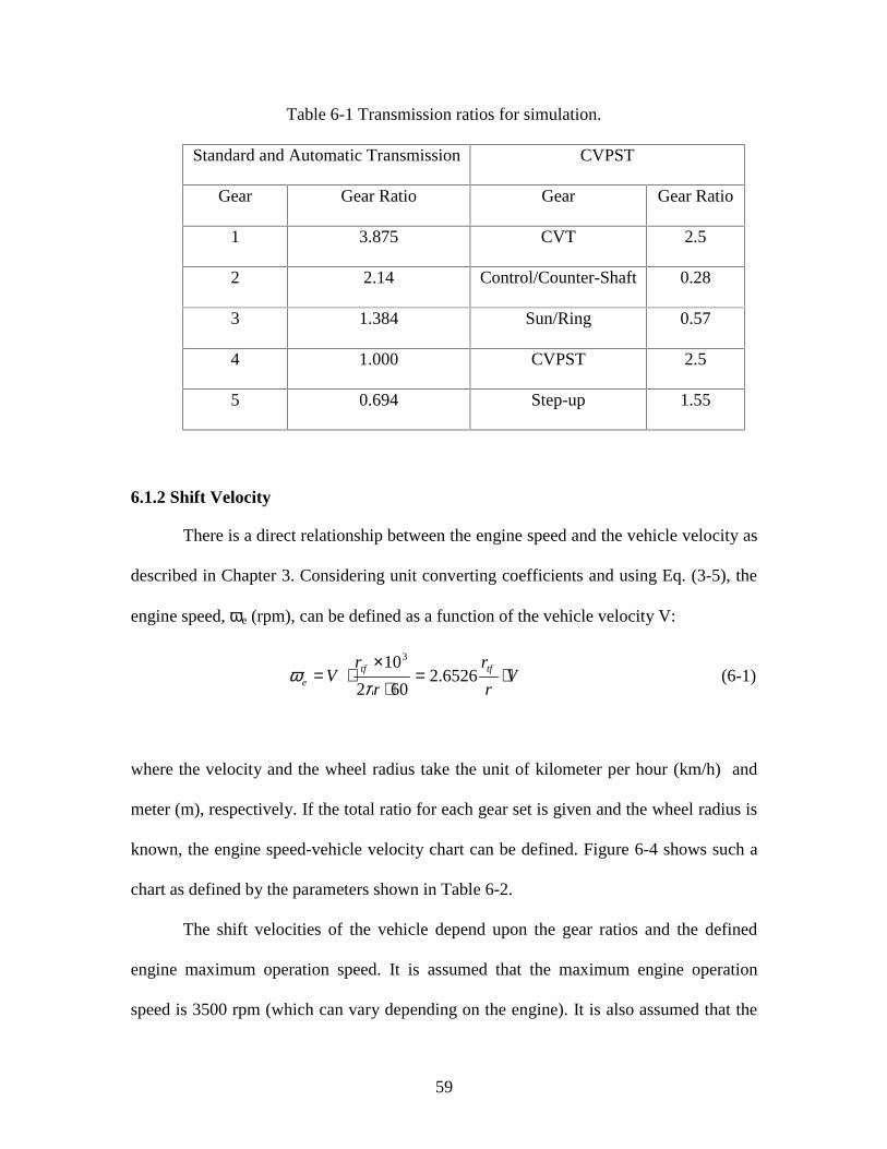
59
Table 6-1 Transmission ratios for simulation.
Standard and Automatic Transmission CVPST
Gear Gear Ratio Gear Gear Ratio
1 3.875 CVT 2.5
2 2.14 Control/Counter-Shaft 0.28
3 1.384 Sun/Ring 0.57
4 1.000 CVPST 2.5
5 0.694 Step-up 1.55
6.1.2 Shift Velocity
There is a direct relationship between the engine speed and the vehicle velocity as
described in Chapter 3. Considering unit converting coefficients and using Eq. (3-5), the
engine speed, ωe (rpm), can be defined as a function of the vehicle velocity V:
Vr
r
r
rV tftf
e ⋅=⋅
×⋅= 6526.2
602
103
πω (6-1)
where the velocity and the wheel radius take the unit of kilometer per hour (km/h) and
meter (m), respectively. If the total ratio for each gear set is given and the wheel radius is
known, the engine speed-vehicle velocity chart can be defined. Figure 6-4 shows such a
chart as defined by the parameters shown in Table 6-2.
The shift velocities of the vehicle depend upon the gear ratios and the defined
engine maximum operation speed. It is assumed that the maximum engine operation
speed is 3500 rpm (which can vary depending on the engine). It is also assumed that the
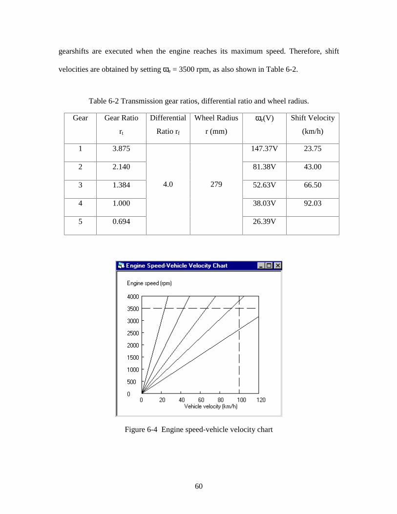
60
gearshifts are executed when the engine reaches its maximum speed. Therefore, shift
velocities are obtained by setting ωe = 3500 rpm, as also shown in Table 6-2.
Table 6-2 Transmission gear ratios, differential ratio and wheel radius.
Gear Gear Ratio
rt
Differential
Ratio rf
Wheel Radius
r (mm)
ωe(V) Shift Velocity
(km/h)
1 3.875 147.37V 23.75
2 2.140 81.38V 43.00
3 1.384 52.63V 66.50
4 1.000 38.03V 92.03
5 0.694
4.0 279
26.39V
Figure 6-4 Engine speed-vehicle velocity chart
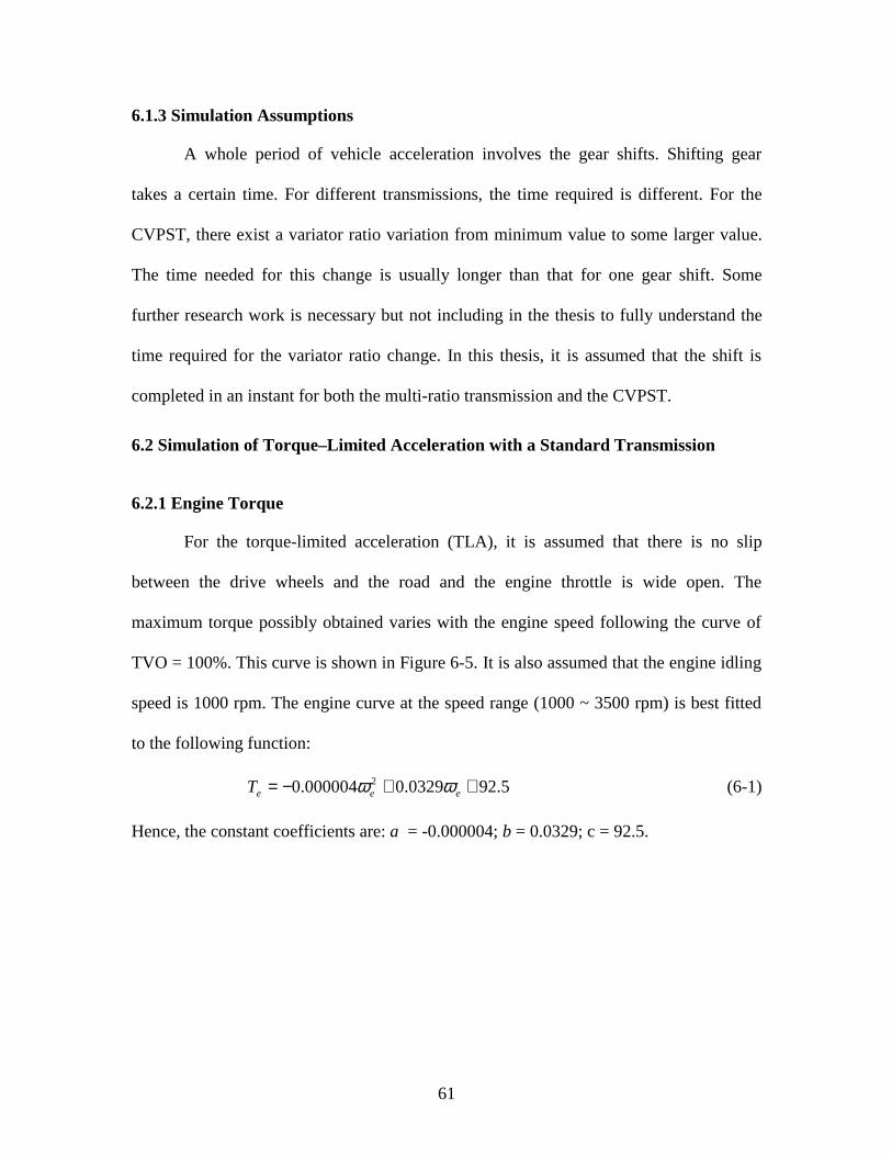
61
6.1.3 Simulation Assumptions
A whole period of vehicle acceleration involves the gear shifts. Shifting gear
takes a certain time. For different transmissions, the time required is different. For the
CVPST, there exist a variator ratio variation from minimum value to some larger value.
The time needed for this change is usually longer than that for one gear shift. Some
further research work is necessary but not including in the thesis to fully understand the
time required for the variator ratio change. In this thesis, it is assumed that the shift is
completed in an instant for both the multi-ratio transmission and the CVPST.
6.2 Simulation of Torque–Limited Acceleration with a Standard Transmission
6.2.1 Engine Torque
For the torque-limited acceleration (TLA), it is assumed that there is no slip
between the drive wheels and the road and the engine throttle is wide open. The
maximum torque possibly obtained varies with the engine speed following the curve of
TVO = 100%. This curve is shown in Figure 6-5. It is also assumed that the engine idling
speed is 1000 rpm. The engine curve at the speed range (1000 ~ 3500 rpm) is best fitted
to the following function:
5.920329.0000004.0 2 ++−= eeeT ωω (6-1)
Hence, the constant coefficients are: a = -0.000004; b = 0.0329; c = 92.5.
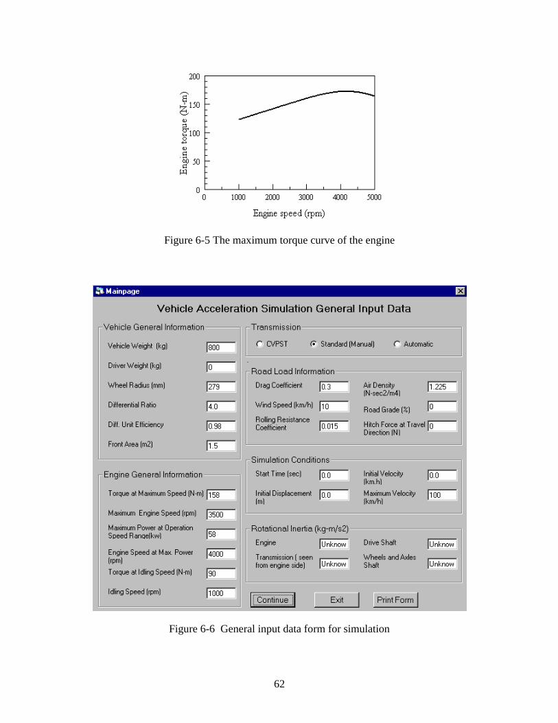
62
Figure 6-5 The maximum torque curve of the engine
Figure 6-6 General input data form for simulation
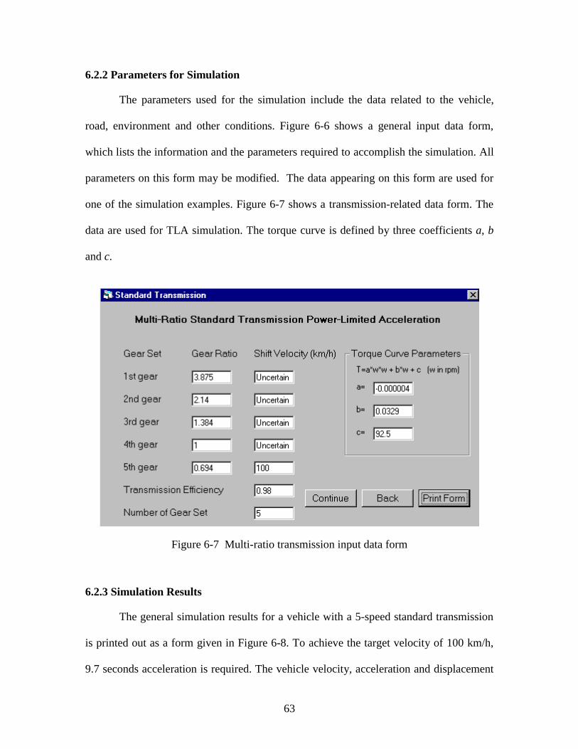
63
6.2.2 Parameters for Simulation
The parameters used for the simulation include the data related to the vehicle,
road, environment and other conditions. Figure 6-6 shows a general input data form,
which lists the information and the parameters required to accomplish the simulation. All
parameters on this form may be modified. The data appearing on this form are used for
one of the simulation examples. Figure 6-7 shows a transmission-related data form. The
data are used for TLA simulation. The torque curve is defined by three coefficients a, b
and c.
Figure 6-7 Multi-ratio transmission input data form
6.2.3 Simulation Results
The general simulation results for a vehicle with a 5-speed standard transmission
is printed out as a form given in Figure 6-8. To achieve the target velocity of 100 km/h,
9.7 seconds acceleration is required. The vehicle velocity, acceleration and displacement
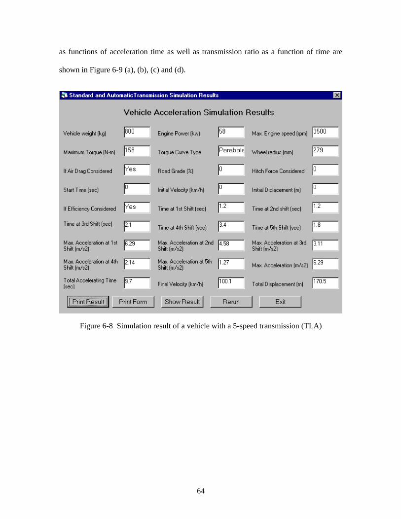
64
as functions of acceleration time as well as transmission ratio as a function of time are
shown in Figure 6-9 (a), (b), (c) and (d).
Figure 6-8 Simulation result of a vehicle with a 5-speed transmission (TLA)
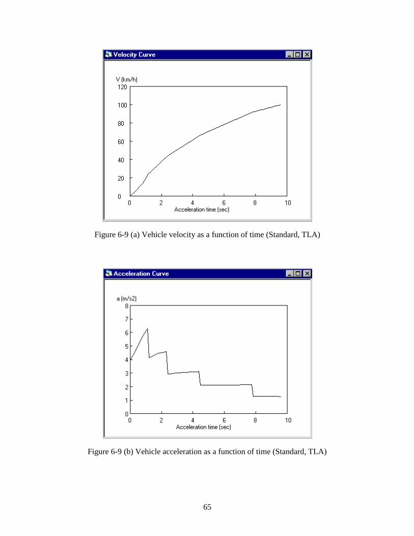
65
Figure 6-9 (a) Vehicle velocity as a function of time (Standard, TLA)
Figure 6-9 (b) Vehicle acceleration as a function of time (Standard, TLA)
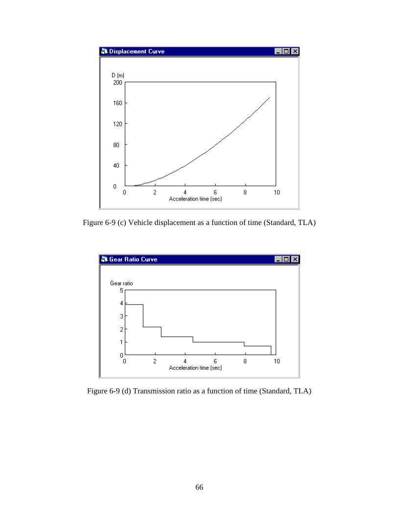
66
Figure 6-9 (c) Vehicle displacement as a function of time (Standard, TLA)
Figure 6-9 (d) Transmission ratio as a function of time (Standard, TLA)
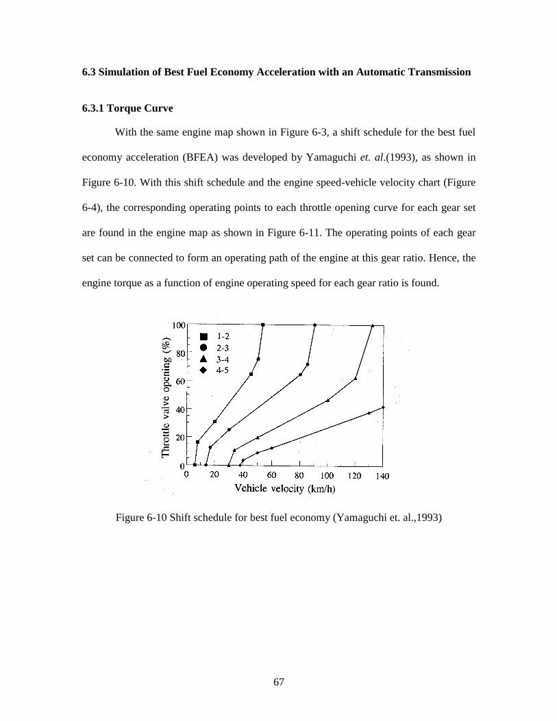
67
6.3 Simulation of Best Fuel Economy Acceleration with an Automatic Transmission
6.3.1 Torque Curve
With the same engine map shown in Figure 6-3, a shift schedule for the best fuel
economy acceleration (BFEA) was developed by Yamaguchi et. al.(1993), as shown in
Figure 6-10. With this shift schedule and the engine speed-vehicle velocity chart (Figure
6-4), the corresponding operating points to each throttle opening curve for each gear set
are found in the engine map as shown in Figure 6-11. The operating points of each gear
set can be connected to form an operating path of the engine at this gear ratio. Hence, the
engine torque as a function of engine operating speed for each gear ratio is found.
Figure 6-10 Shift schedule for best fuel economy (Yamaguchi et. al.,1993)
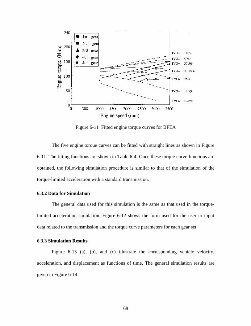
68
Figure 6-11 Fitted engine torque curves for BFEA
The five engine torque curves can be fitted with straight lines as shown in Figure
6-11. The fitting functions are shown in Table 6-4. Once these torque curve functions are
obtained, the following simulation procedure is similar to that of the simulation of the
torque-limited acceleration with a standard transmission.
6.3.2 Data for Simulation
The general data used for this simulation is the same as that used in the torque-
limited acceleration simulation. Figure 6-12 shows the form used for the user to input
data related to the transmission and the torque curve parameters for each gear set.
6.3.3 Simulation Results
Figure 6-13 (a), (b), and (c) illustrate the corresponding vehicle velocity,
acceleration, and displacement as functions of time. The general simulation results are
given in Figure 6-14.
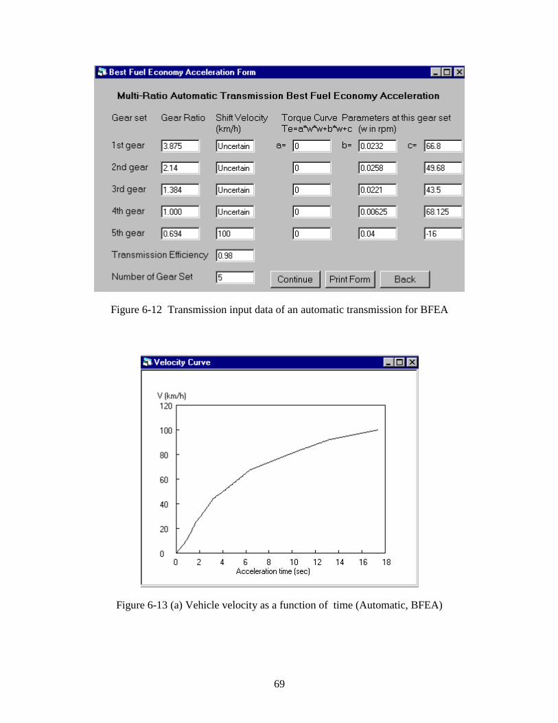
69
Figure 6-12 Transmission input data of an automatic transmission for BFEA
Figure 6-13 (a) Vehicle velocity as a function of time (Automatic, BFEA)
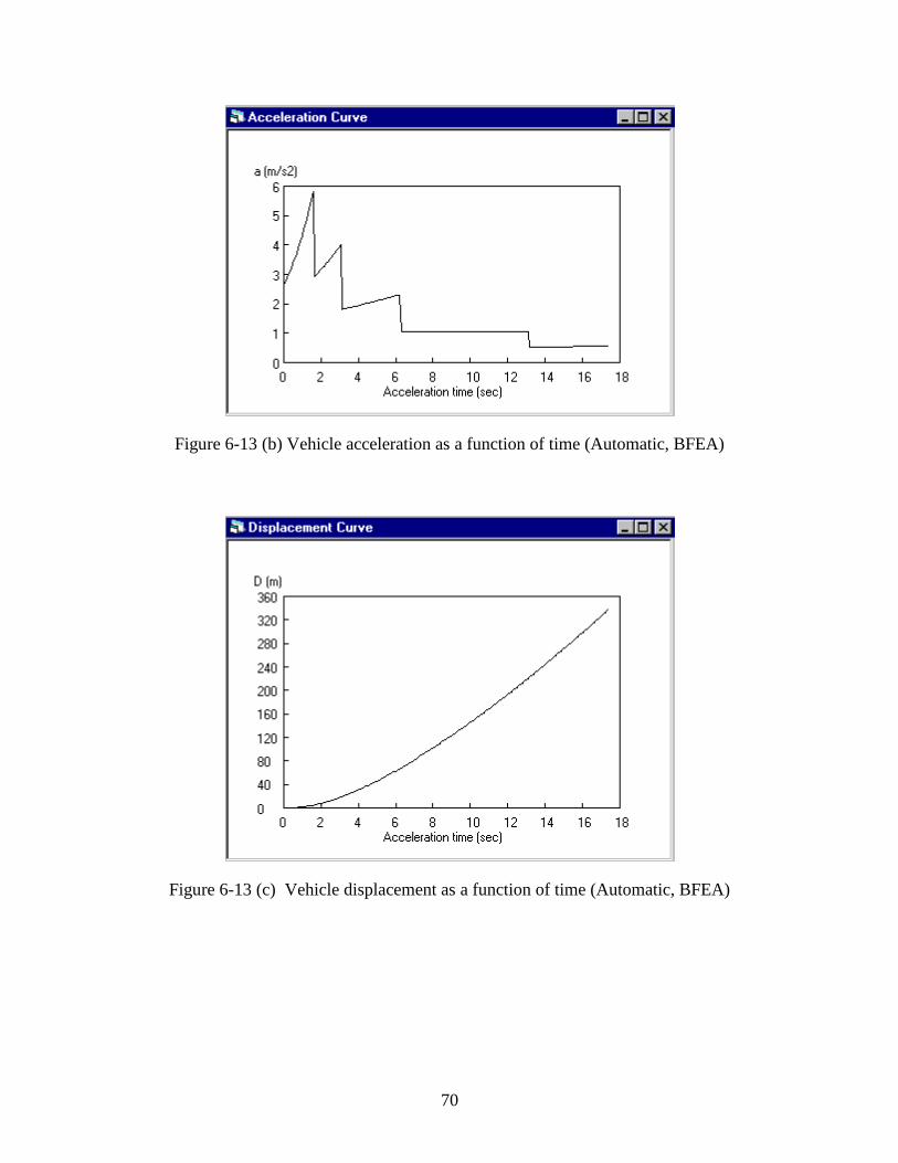
70
Figure 6-13 (b) Vehicle acceleration as a function of time (Automatic, BFEA)
Figure 6-13 (c) Vehicle displacement as a function of time (Automatic, BFEA)
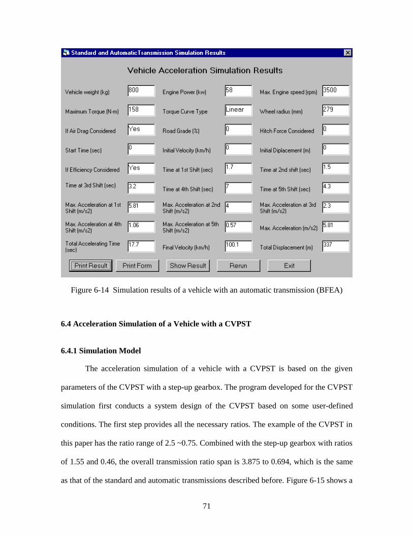
71
Figure 6-14 Simulation results of a vehicle with an automatic transmission (BFEA)
6.4 Acceleration Simulation of a Vehicle with a CVPST
6.4.1 Simulation Model
The acceleration simulation of a vehicle with a CVPST is based on the given
parameters of the CVPST with a step-up gearbox. The program developed for the CVPST
simulation first conducts a system design of the CVPST based on some user-defined
conditions. The first step provides all the necessary ratios. The example of the CVPST in
this paper has the ratio range of 2.5 ~0.75. Combined with the step-up gearbox with ratios
of 1.55 and 0.46, the overall transmission ratio span is 3.875 to 0.694, which is the same
as that of the standard and automatic transmissions described before. Figure 6-15 shows a
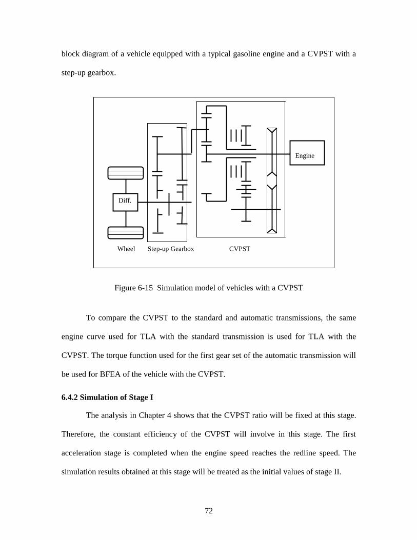
72
block diagram of a vehicle equipped with a typical gasoline engine and a CVPST with a
step-up gearbox.
Figure 6-15 Simulation model of vehicles with a CVPST
To compare the CVPST to the standard and automatic transmissions, the same
engine curve used for TLA with the standard transmission is used for TLA with the
CVPST. The torque function used for the first gear set of the automatic transmission will
be used for BFEA of the vehicle with the CVPST.
6.4.2 Simulation of Stage I
The analysis in Chapter 4 shows that the CVPST ratio will be fixed at this stage.
Therefore, the constant efficiency of the CVPST will involve in this stage. The first
acceleration stage is completed when the engine speed reaches the redline speed. The
simulation results obtained at this stage will be treated as the initial values of stage II.
Wheel Step-up Gearbox CVPST
Engine
Diff.
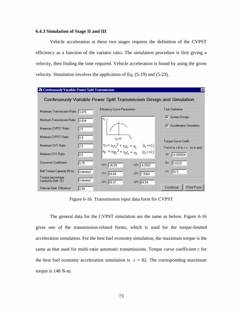
73
6.4.3 Simulation of Stage II and III
Vehicle acceleration at these two stages requires the definition of the CVPST
efficiency as a function of the variator ratio. The simulation procedure is first giving a
velocity, then finding the time required. Vehicle acceleration is found by using the given
velocity. Simulation involves the application of Eq. (5-19) and (5-23).
Figure 6-16 Transmission input data form for CVPST
The general data for the CVPST simulation are the same as before. Figure 6-16
gives one of the transmission-related forms, which is used for the torque-limited
acceleration simulation. For the best fuel economy simulation, the maximum torque is the
same as that used for multi-ratio automatic transmissions. Torque curve coefficient c for
the best fuel economy acceleration simulation is c = 82. The corresponding maximum
torque is 148 N-m.
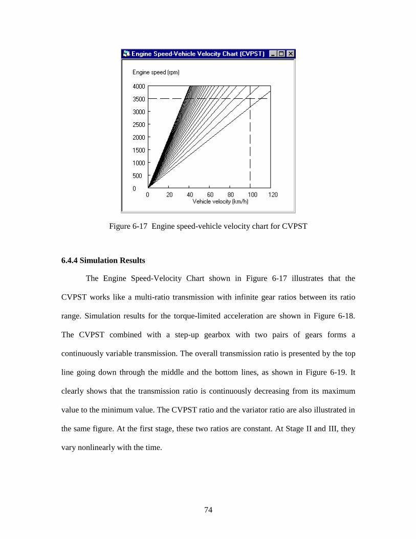
74
Figure 6-17 Engine speed-vehicle velocity chart for CVPST
6.4.4 Simulation Results
The Engine Speed-Velocity Chart shown in Figure 6-17 illustrates that the
CVPST works like a multi-ratio transmission with infinite gear ratios between its ratio
range. Simulation results for the torque-limited acceleration are shown in Figure 6-18.
The CVPST combined with a step-up gearbox with two pairs of gears forms a
continuously variable transmission. The overall transmission ratio is presented by the top
line going down through the middle and the bottom lines, as shown in Figure 6-19. It
clearly shows that the transmission ratio is continuously decreasing from its maximum
value to the minimum value. The CVPST ratio and the variator ratio are also illustrated in
the same figure. At the first stage, these two ratios are constant. At Stage II and III, they
vary nonlinearly with the time.
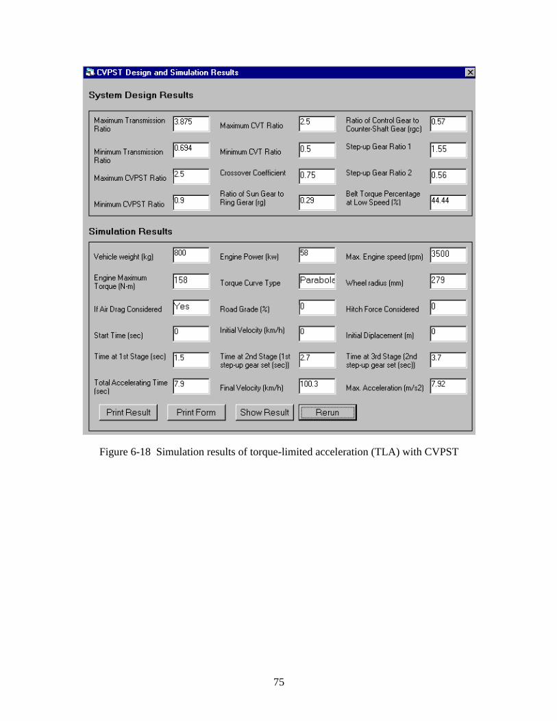
75
Figure 6-18 Simulation results of torque-limited acceleration (TLA) with CVPST
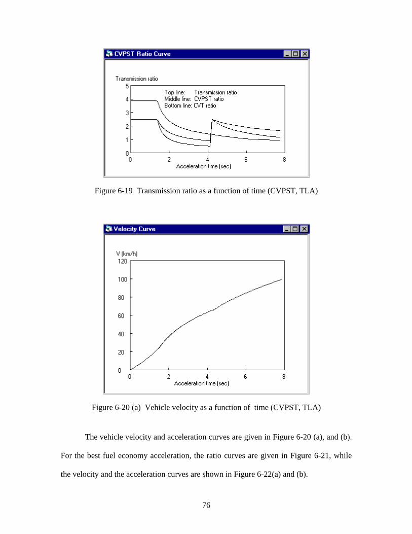
76
Figure 6-19 Transmission ratio as a function of time (CVPST, TLA)
Figure 6-20 (a) Vehicle velocity as a function of time (CVPST, TLA)
The vehicle velocity and acceleration curves are given in Figure 6-20 (a), and (b).
For the best fuel economy acceleration, the ratio curves are given in Figure 6-21, while
the velocity and the acceleration curves are shown in Figure 6-22(a) and (b).
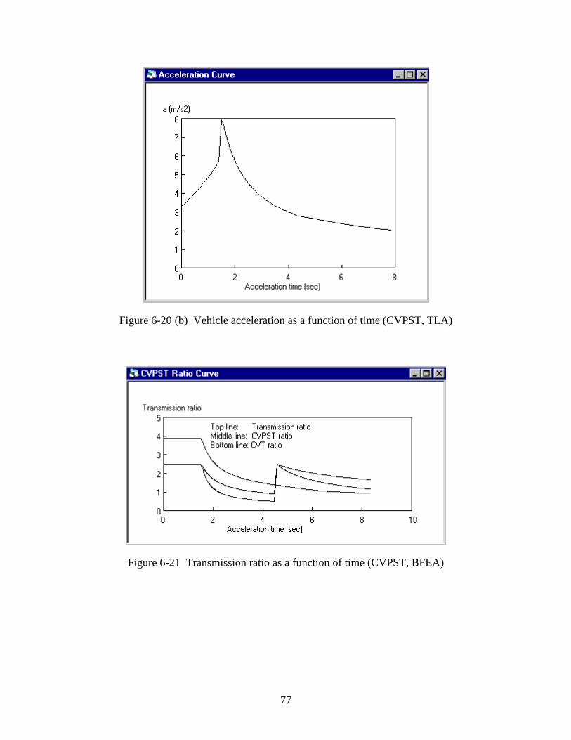
77
Figure 6-20 (b) Vehicle acceleration as a function of time (CVPST, TLA)
Figure 6-21 Transmission ratio as a function of time (CVPST, BFEA)
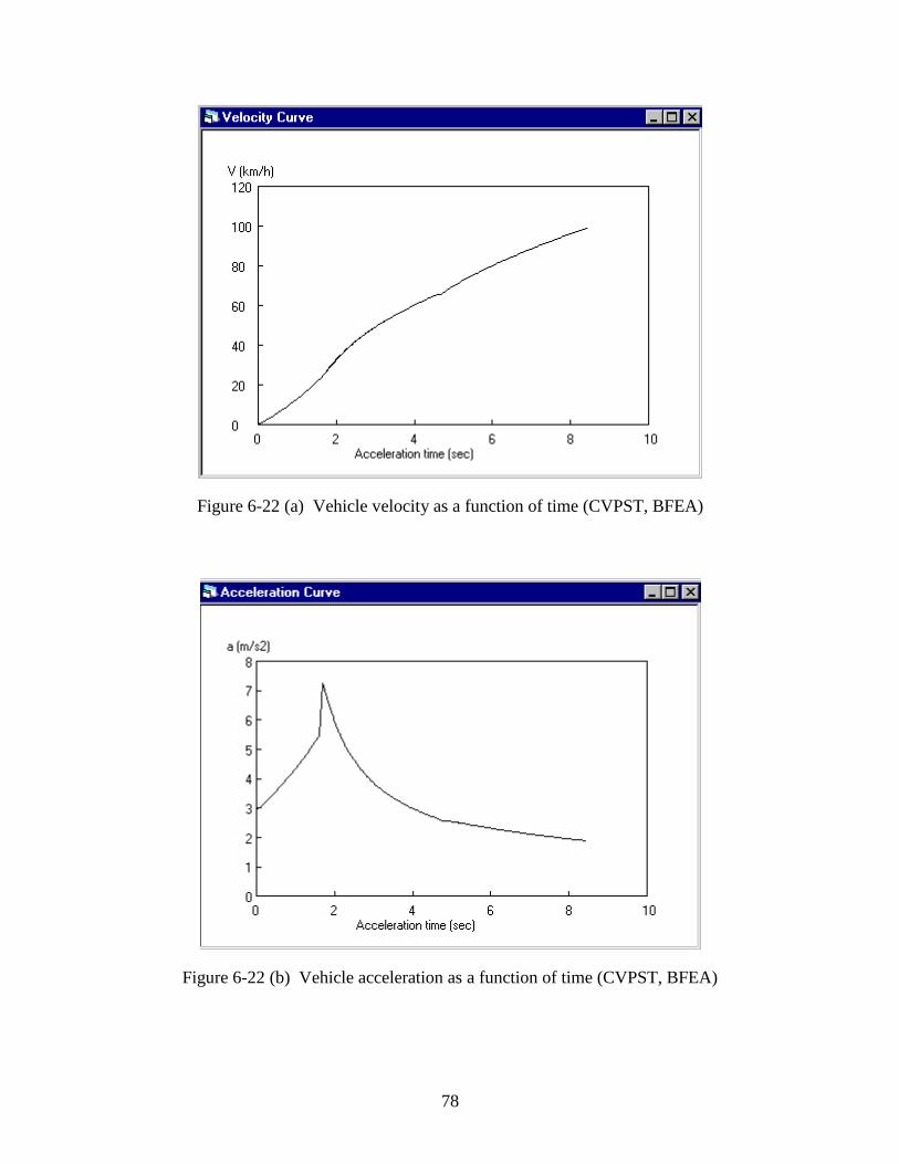
78
Figure 6-22 (a) Vehicle velocity as a function of time (CVPST, BFEA)
Figure 6-22 (b) Vehicle acceleration as a function of time (CVPST, BFEA)
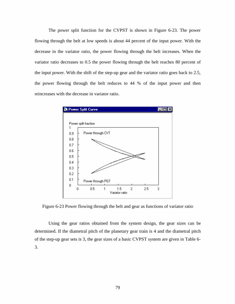
79
The power split function for the CVPST is shown in Figure 6-23. The power
flowing through the belt at low speeds is about 44 percent of the input power. With the
decrease in the variator ratio, the power flowing through the belt increases. When the
variator ratio decreases to 0.5 the power flowing through the belt reaches 80 percent of
the input power. With the shift of the step-up gear and the variator ratio goes back to 2.5,
the power flowing through the belt reduces to 44 % of the input power and then
reincreases with the decrease in variator ratio.
Figure 6-23 Power flowing through the belt and gear as functions of variator ratio
Using the gear ratios obtained from the system design, the gear sizes can be
determined. If the diametral pitch of the planetary gear train is 4 and the diametral pitch
of the step-up gear sets is 3, the gear sizes of a basic CVPST system are given in Table 6-
3.
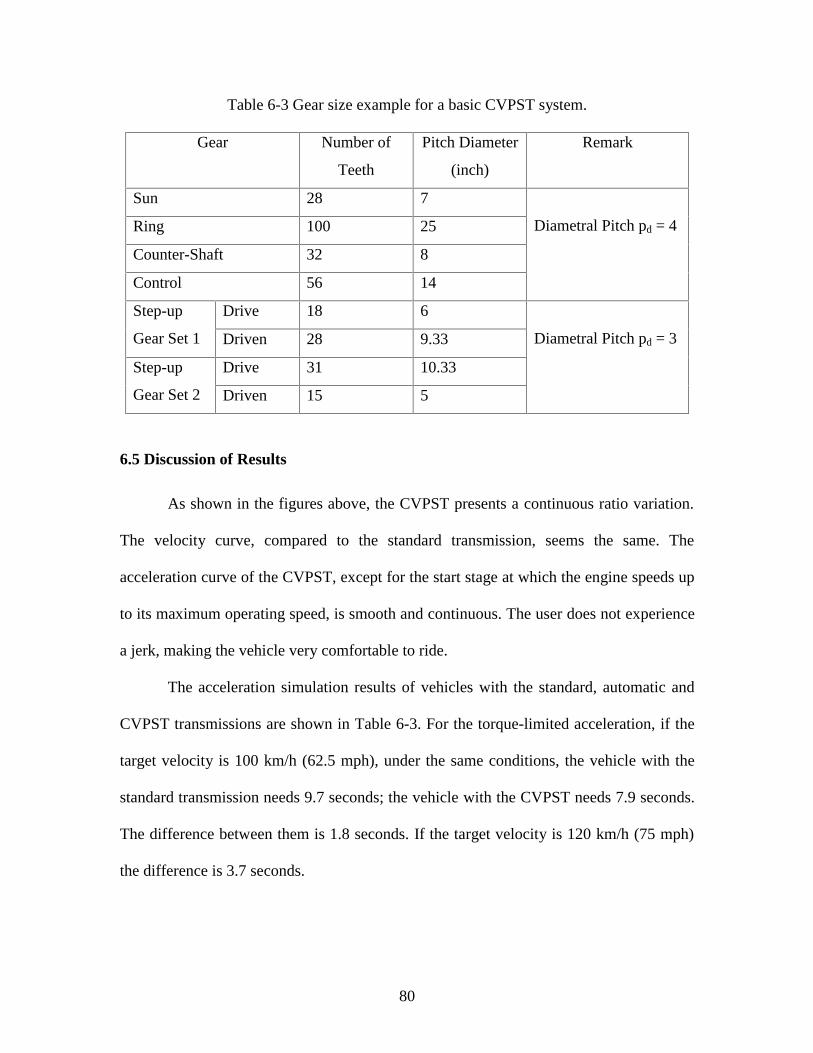
80
Table 6-3 Gear size example for a basic CVPST system.
Gear Number of
Teeth
Pitch Diameter
(inch)
Remark
Sun 28 7
Ring 100 25
Counter-Shaft 32 8
Control 56 14
Diametral Pitch pd = 4
Drive 18 6Step-up
Gear Set 1 Driven 28 9.33
Drive 31 10.33Step-up
Gear Set 2 Driven 15 5
Diametral Pitch pd = 3
6.5 Discussion of Results
As shown in the figures above, the CVPST presents a continuous ratio variation.
The velocity curve, compared to the standard transmission, seems the same. The
acceleration curve of the CVPST, except for the start stage at which the engine speeds up
to its maximum operating speed, is smooth and continuous. The user does not experience
a jerk, making the vehicle very comfortable to ride.
The acceleration simulation results of vehicles with the standard, automatic and
CVPST transmissions are shown in Table 6-3. For the torque-limited acceleration, if the
target velocity is 100 km/h (62.5 mph), under the same conditions, the vehicle with the
standard transmission needs 9.7 seconds; the vehicle with the CVPST needs 7.9 seconds.
The difference between them is 1.8 seconds. If the target velocity is 120 km/h (75 mph)
the difference is 3.7 seconds.
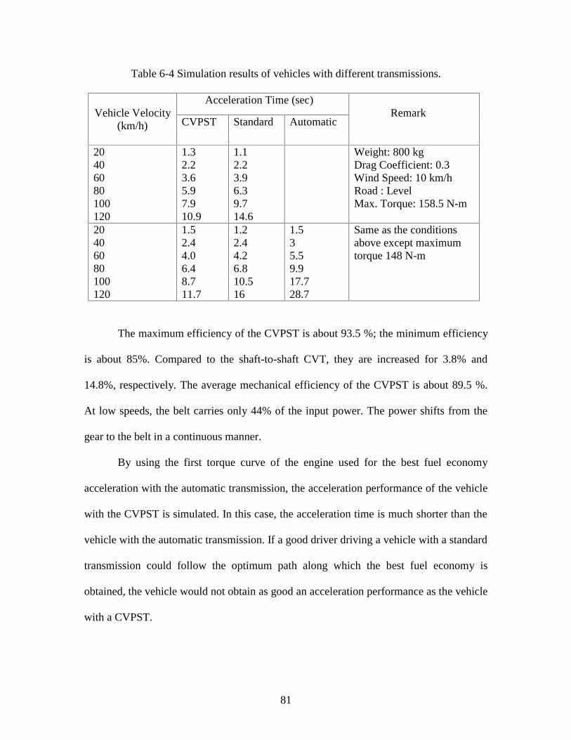
81
Table 6-4 Simulation results of vehicles with different transmissions.
Acceleration Time (sec)Vehicle Velocity
(km/h) CVPST Standard Automatic Remark
20406080100120
1.32.23.65.97.910.9
1.12.23.96.39.714.6
Weight: 800 kgDrag Coefficient: 0.3Wind Speed: 10 km/hRoad : LevelMax. Torque: 158.5 N-m
20406080100120
1.52.44.06.48.711.7
1.22.44.26.810.516
1.535.59.917.728.7
Same as the conditionsabove except maximumtorque 148 N-m
The maximum efficiency of the CVPST is about 93.5 %; the minimum efficiency
is about 85%. Compared to the shaft-to-shaft CVT, they are increased for 3.8% and
14.8%, respectively. The average mechanical efficiency of the CVPST is about 89.5 %.
At low speeds, the belt carries only 44% of the input power. The power shifts from the
gear to the belt in a continuous manner.
By using the first torque curve of the engine used for the best fuel economy
acceleration with the automatic transmission, the acceleration performance of the vehicle
with the CVPST is simulated. In this case, the acceleration time is much shorter than the
vehicle with the automatic transmission. If a good driver driving a vehicle with a standard
transmission could follow the optimum path along which the best fuel economy is
obtained, the vehicle would not obtain as good an acceleration performance as the vehicle
with a CVPST.
82
For the best fuel economy acceleration, the engine of the vehicle with a CVPST
operates at the best efficiency range, except for the start stage. Due to the shifts, the
engine of a vehicle with a standard or an automatic transmission has to work following a
zigzag path, thus it is impossible to stay at the optimum range. The better fuel economy
for the vehicle with a CVPST is obvious.
6.6 Conclusion
The vehicle acceleration simulation displays that the CVPST can provide a
continuously variable ratio change and thus a smooth and continuous acceleration
change. It is more comfortable for the driver and the passengers to ride a vehicle
equipped with a CVPST. The simulation of the vehicle acceleration performance presents
that both the driveability and the fuel economy for the vehicle with a CVPST are better
than the one with a standard or a multi-ratio automatic transmission. A power split
function is available for the CVPST which expands the power capacity of the belt CVT.
At low speeds, the belt only carries part of the input power. A required power split
percentage is obtained by using the computer program to accomplish the system design.
It is possible to shift the power flow in the system from the gear to the CVT unit in a
continuous manner.
6.7 Future Recommendations
The simulation of the CVPST uses the fitted function of the power loss curve.
This curve is obtained under certain conditions. The next phase of this study should pay
attention to the study of power loss of the belt CVT, especially the loss at both entrance
and exit of both the primary and secondary pulleys. The study should also find the inertia
variation of the CVPST due to the variator ratio change. Since the variator ratio changes
83
nonlinearly during the acceleration, an electric control system is strongly recommended.
Another valuable work is to develop a prototype control system which meets the
operation requirement.
84
REFERENCES
Ashley, Steven, 1994, “Is CVT the car transmission of the future?”, MechanicalEngineering, Nov. 1994, pp.64-68
Avramidis, Stanley, “A ‘state of the art’ chain driven CVT design,” SAE TransactionsVol. 95 (1986), SAE Technical Paper No. 861354
Bent, D. J., 1981, “Axial force and efficiency tests of fixed center variable speed beltdrive,” SAE Paper 810103
Bonthron, Anders, “CVT-efficiency measured under dynamic running conditions,” SAETechnical Paper No. 850569
Bowling, Bruce, 1997, “Vehicle acceleration program,” http://sura1.jlab.org/~bowling/autosim_f.html
Chana, Howard E., “Performance of CVT transmissions,” SAE Transactions Vol. 95(1986), SAE Technical Paper No. 860637
Chen, T. F., Lee, D. W. and Sung, C. K., 1995, “An experimental study on transmissionefficiency of a rubber belt continuous variable transmission (CVT),” 9th IFToMMConference Proceedings, Vol. 1, pp. 652-657
Cook, Jhon F., 1975, “Continuously variable gear ratio automatic transmission,” US.Patent No. 3,899,190, Aug. 19, 1975
Cowan, Ben, 1992, “Variable speed transmission,” U.S Patent No. 5,167,591, Dce. 1,1992
Cowan, Ben, 1993, “Variable speed transmission,” U.S Patent No. 5,215,323, Jun. 1,1993
Fitz, Frank A.; Pires, Paul B., “A high torque, high efficiency CVT for electric vehicles”,SAE Technical Paper No. 910251
Fujii, Toru; Kusano, Takayuki; Takahashi, Mitsuhiko; Kiji, Takafumi, “Study on forcestransmitting between pulleys and blocks of a block-type CVT belt,” SAE Technical PaperNo. 921746
Fujii, T., Kurokawa, T. and Kanehara, S., 1993, “A study of a metal pushing V-belt typeCVT-Part1: relation between transmitted torque and pulley thrust,” SAE paper 930666
85
Fujii, T., Kurokawa, T. and Kanehara, S., 1993, “A study of a metal pushing V-belt typeCVT-Part 2: compression force between metal blocks and ring tension,” SAE paper930667
Furumoto, Mitsumasa et. al., 1990, “Hydraulically operated continuously variabletransmission,” US. Patent No. 4,939,900, July 10, 1990
Gillespie, T. D., 1992, “Fundamentals of vehicle dynamics,” SAE, Ch. 1-4.
Guebeli, J. D. Micklem, C. R. Burrows, 1993, “Maximum transmission efficiency of asteel belt continuously variable transmission,” Transactions of the ASME, Vol. 115,December 1993, pp.1044~1048.
Guo, Z. Y.; Yang, X. C.; Yang, D.; Frank, A. A., 1988, “On obtaining the best fueleconomy and performance for vehicles with engine-CVT transmissions,” SAE TechnicalPaper No. 881735
Hanses, Markus H., 1997, “Friction and pressure analysis on the driving sheaves of a beltCVT,” Masters thesis, West Virginia University
Hendriks, E., 1993, “Qualitative and Quantitative Influence of a Fully ElectronicallyControlled CVT on Fuel Economy and Vehicle Performance,” SAE Paper 930668
Hendriks, Emery; ter Heegde, Paul; van Prooijen, Tom, 1988, “Aspects of a metalpushing v-belt for automotive cut application,” SAE Transactions Vol. 97 (1988), SAETechnical Paper No. 881734
Hendriks, E. and Heeze NR, “Continuously variable transmissions provided with a torqueconverter,” U.S Patent No. 5,048,371, Sept. 17, 1991
Hibi, Toshifumi, 1993, “Friction roller type continuously variable transmissions,” U.SPatent No. 5,230,670, July 27, 1993 and No. 5,267,920, Dec. 7, 1993
Hsieh, L. and Yan, H., 1990, “On the mechanical efficiency of continuously variabletransmissions with planetary gear trains,” Int. J. of Vehicle Design, Vol 11, No. 2, pp.177-187
Inoue, Kazuo, 1990, “Hydrostatically operated continuously variable transmission,” US.Patent No. 4,967,556, Nov. 6, 1990
Ishibashi, Yoichi; Kitamoto, Hiroaki, “Improvement of fuel consumption of two-strokeengines applying CVT,” SAE Technical Paper No. 891752
Kawahara, Eiichiro et. al., 1990, “Hydraulically operated continuously variabletransmission,” U.S Patent No. 4,944,154, July 31, 1990
86
Kawamoto Mitsumi, 1985, “Continuously variable speed transmission for motorvehicles,” U.S Patent No. 4,550,629, Nov. 5, 1985
Kumm, Emerson L.and Kraver, Theodore C., 1986, “Enhancement of the flat-belt,continuously-variable transmission technology,” SAE Transactions Vol. 95 (1986), SAETechnical Paper No. 861214
Kumm, Emerson L., 1991, “Continuously variable transmission using planetary gearingwith regenerative torque transfer and employing belt slip to measure and control pulleytorque, ” U.S Patent No. 5,011,458, April, 30, 1991
Lemmens, John, 1974, “Continuously variable automatic transmission,” U.S Patent No.3,850,050, Nov. 26, 1974
Lemmens, John, 1972, “Variable speed transmission,” U.S Patent No. 3,641,843, Feb. 15,1972
Mabie, Hanilton H. and Reinholtz, Charles F., 1987, “Mechanisms and Dynamics ofMachinery,” 4th Edition, John Wiley & Sons, Inc.
Moroto, Suzo et. al., “Continuously variable speed transmission for a vehicle having aforward-reverse changeover mechanism,” U.S Patent No. 4,602,525, July 29, 1986
Mucino, V. H., Smith, J. E., Shama, P. K., Cowan, B. and Kmicikiewicz, M., 1995, “Adouble planetary gear train-CVT transmission with multiple applications, ” SAETechnical Paper No. 950094
Mucino, V. H., Smith, J. E., Cowan, B. and Kmicikiewicz, M., “A continuously variablepower split transmission for automotive applications, ” SAE Technical Paper No. 970687
Nakano, Masaki; Hibi, Toshifumi; Kobayashi, Katsuya, “Dual-cavity half toroidal CVTfor passenger cars,” SAE Technical Paper No. 922105
Orshansky, Eli, Huntley, Peter and Weseloh, William E., 1974, “Automobile fueleconomy with hydromechanical transmission by simulation studies,” SAE TechnicalPaper No. 740308
Palmer, R. S. J. and Bear, J. H. F., 1997, “Mechanical efficiency of a variable speed,fixed center V-belt drive,” ASAE Transactions, J of Engineering for Industry, pp. 771-779
Phillips, Andrew W., Assanis, Deennis N. and Badgley, Patric, 1990, “Development anduse of a vehicle powertrain simulation for fuel economy and performance studies,” SAETechnical Paper No. 900619
87
Radtke, R. R.; Unnewehr, L. E.; Freedman, R. J., “Optimization of a ContinuouslyVariable Transmission with emission constraints,” SAE Transactions Vol. 90 (1981),SAE Technical Paper No. 810107
Robins, Francis B., 1993, “Continuously variable transmission,” U.S Patent No.5,183,444, Feb. 2, 1993
Schwab, Manfred, 1990, “Electronically-controlled transmission systems—currentposition and future developments,” SAE Technical Paper No. 901156
Takayama et. al, 1990, “Continuously variable transmission,” U.S Patent No. 5,050,457,Sep. 24, 1991
Tanaka, Hirohisa and Imanishi, Takashi, 1994, “Toroidal type continuously variabletransmission,” U.S Patent No. 5,303,796, April 19, 1994
Thompson, Andrew C.; Lipman, John M., “The Lotus CVT and evolution of the smarttransmission concept,” SAE Technical Paper No. 922106
Won, Yuen Vann, 1989, “Continuously variable gear drive transmissions,” U.S Paten No.4,854,190, Aug. 8, 1989
Yamaguchi, Jack, “Global Viewpoints: Honda Civic,” Automotive Engineering,November 1995, pp.88~93.
Yuki, Tsukasa, Takayama, Mitsunao and Kato Hisato, “Development of dry hybrid beltCVT, ” JSAE Review 16,1995, pp.251~256.
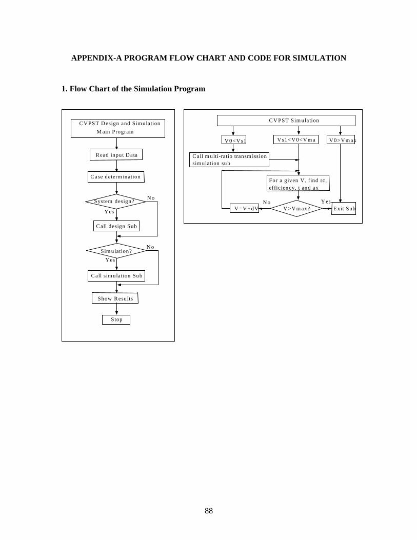
88
APPENDIX-A PROGRAM FLOW CHART AND CODE FOR SIMULATION
1. Flow Chart of the Simulation Program
Read input D ata
Case determ ination
Call design Sub
Sim ulation?
Call simulation Sub
System design?
Stop
N o
N o
Y es
Y es
Show Results
C V PST D esign and Simulation
M ain Program
V 0>V m axV 0<V s1 V s1<V 0<V m a
sim ulation subCall m ulti-ratio transm ission
CV PST Sim ulation
efficiency, t and axFor a given V , find rc,
V >V m ax?Y esN o
V =V +dV Exit Sub
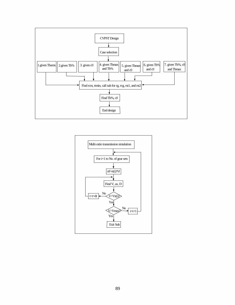
89
Multi-ratio transmission simulation
For i=1 to No. of gear sets
Find V, ax, D
t=t+dt
Yes
NoV>Vs(i)?
V>Vmax? i=i+1No
Yes
Exit Sub
rtf=rt(i)*rf
1.given Tbamx 2.given Tb% 3. given c0and Tb%
4. given Tbmax 5. given Tbmaxand c0 and c0
6. given Tb%and Tbmax
7. given Tb%, c0
Find rcm, rtmin, call sub for rg, rcg, rst1, and rst2
Case selection
CVPST Design
Find Tb%, c0
End design
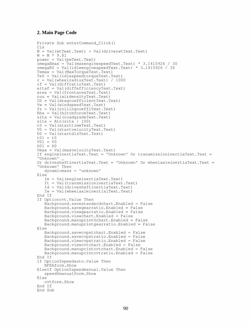
90
2. Main Page Code
Private Sub enterCommand_Click()ClsM = Val(wtText.Text) + Val(driverwtText.Text)W = M * 9.81power = Val(pwText.Text)omegaEmax = Val(maxenginespeedText.Text) * 3.1415926 / 30omegaE0 = Val(idleenginespeedText.Text) * 3.1415926 / 30Temax = Val(MaxTorqueText.Text)Te0 = Val(idlespeedtorqueText.Text)r = Val(wheelradiusText.Text) / 1000rf = Val(diffratioText.Text)eitaf = Val(diffefficiencyText.Text)area = Val(frontareaText.Text)rou = Val(airdensityText.Text)CD = Val(dragcoefficientText.Text)Vw = Val(windspeedText.Text)fr = Val(rollingcoeffiText.Text)Rhx = Val(hitchforceText.Text)sita = Val(roadgradeText.Text)sita = Atn(sita / 100)t0 = Val(starttimeText.Text)V0 = Val(startvelocityText.Text)D0 = Val(startdisText.Text)t01 = t0V01 = V0D01 = D0Vmax = Val(maxvelocityText.Text)If engineinertiaText.Text = "Unknown" Or transmissioninertiaText.Text ="Unknown" _Or driveshaftinertiaText.Text = "Unknown" Or wheelaxleinertiaText.Text ="Unknown" Then dynamicmass = "unknown"Else Ie = Val(engineinertiaText.Text) It = Val(transmissioninertiaText.Text) Id = Val(driveshaftinertiaText.Text) Iw = Val(wheelaxleinertialText.Text)End IfIf Optioncvt.Value Then Background.savestandardchart.Enabled = False Background.savegearratio.Enabled = False Background.viewgearratio.Enabled = False Background.viewchart.Enabled = False Background.manuprintGchart.Enabled = False Background.manuprintgearratio.Enabled = FalseElse Background.savecvpstchart.Enabled = False Background.savecvpstratio.Enabled = False Background.viewcvpstratio.Enabled = False Background.viewcvtchart.Enabled = False Background.manuprintcvtchart.Enabled = False Background.manuprintcvtratio.Enabled = FalseEnd IfIf Option5speedauto.Value Then BFEAform.ShowElseIf Option5speedmanual.Value Then speed5manualform.ShowElse cvtform.ShowEnd IfEnd Sub
91
3. Code for CVPST Design and Simulation
(1) Main program
Private Sub enterCommand_Click()rtotalmax = Val(ratioText(1).Text)rtotalmin = Val(ratioText(2).Text)rtmax = Val(ratioText(3).Text)rtmin = Val(ratioText(4).Text)rcmax = Val(ratioText(5).Text)rcmin = Val(ratioText(6).Text)eitagear = Val(stepupgearefficiencyText.Text)S1 = Val(s1Text.Text) / 100S2 = Val(s2Text.Text) / 100N1 = Val(n1Text.Text) / 100N2 = Val(n2Text.Text) / 100U1 = Val(u1Text.Text) / 100U2 = Val(u2Text.Text) / 100a = Val(aText.Text) * (30 / 3.1416) ^ 2b = Val(bText.Text) * 30 / 3.1416cc = Val(cText.Text)TTmax = a * omegaEmax ^ 2 + b * omegaEmax + ccIf rtotalmax <= rtotalmin Or rtmax <= rtmin Or rcmax <= rcmin Oreitagear > 1 Then MsgBox "You typed invalid value(s)!" Unload Me Load MeEnd IfIf belttorqueText.Text = "Unlimited" And torquepercentageText.Text ="Unlimited" _And crossovercoefficientText.Text = "Unknown" Then case1 = 0ElseIf belttorqueText.Text <> "Unlimited" And torquepercentageText.Text= "Unlimited" _And crossovercoefficientText.Text = "Unknown" Then case1 = 1ElseIf belttorqueText.Text = "Unlimited" And torquepercentageText.Text<> "Unlimited" _And crossovercoefficientText.Text = "Unknown" Then case1 = 2ElseIf belttorqueText.Text = "Unlimited" And torquepercentageText.Text ="Unlimited" _And crossovercoefficientText.Text <> "Unknown" Then case1 = 3ElseIf belttorqueText.Text <> "Unlimited" And torquepercentageText.Text<> "Unlimited" _And crossovercoefficientText.Text = "Unknown" Then case1 = 4ElseIf belttorqueText.Text <> "Unlimited" And torquepercentageText.Text= "Unlimited" _And crossovercoefficientText.Text <> "Unknown" Then case1 = 5ElseIf belttorqueText.Text = "Unlimited" And torquepercentageText.Text<> "Unlimited" _And crossovercoefficientText.Text <> "Unknown" Then case1 = 6Else case1 = 7End If
If crossovercoefficientText.Text <> "Unknown" Then
92
If Val(crossovercoefficientText.Text) >= 1 OrVal(crossovercoefficientText.Text) <= 0 Then
MsgBox "Invalid crossover value!" Unload Me Me.Show Exit Sub Else c0 = Val(crossovercoefficientText.Text) End IfEnd IfIf belttorqueText.Text <> "Unlimited" Then If Val(belttorqueText.Text) <= 0 Then MsgBox "Invalid belt torque value!" Unload Me Me.Show Exit Sub Else Tbmax = Val(belttorqueText.Text) End IfEnd IfIf torquepercentageText.Text <> "Unlimited" Then If Val(torquepercentageText.Text) <= 0 OrVal(torquepercentageText.Text) >= 100 Then MsgBox "Invalid belt torque percentage value!" Unload Me Me.Show Exit Sub Else Tbpercent = Val(torquepercentageText.Text) / 100 End IfEnd IfIf case1 = 0 Then Call designsubSub rcm = rcmax * rcmin * (rtmin - rtmax) / (rtmax * rcmin - rcmax *rtmin) c0 = (rcm - rcmin) / (rcmax - rcmin) Tbpercent = rcg / (rcmax * rg + rcg)End IfIf designCheck.Value Then Call cvpstdesignSub’ End Design
’Start Simulationrtf = rf * rst1 * rcmax * (1 + rg) / (rcmax * rg + rcg)If dynamicmass = "unknown" Then ’no inertia known K = 1.04 + 0.0025 * rtf * rtfElse K = (M + ((Ie + It) * rtf * rtf + Id * rf * rf + Iw) / r / r) / MEnd IfIf simulationCheck.Value Then Call calculation3Sub Call cvpstsimusub2End Ifresult2Form.ShowEnd Sub
(2) CVPST Design
Sub cvpstdesignSub()Dim rcm1 As SingleSelect Case case1Case 1 Tcvt = Tbmax Tpgt = Temax - Tcvt rcm = rcmax * Tcvt / Tpgt
93
rtmin = rcmin / rcmax * (rcm + rcmax) * rtmax / (rcm + rcmin) Call designsubSub c0 = (rcm - rcmin) / (rcmax - rcmin) Tbpercent = rcg / (rcmax * rg + rcg)Case 2 Tcvt = Temax * Tbpercent Tpgt = Temax - Tcvt rcm = rcmax * Tcvt / Tpgt rtmin = rcmin / rcmax * (rcm + rcmax) * rtmax / (rcm + rcmin) Call designsubSub c0 = (rcm - rcmin) / (rcmax - rcmin) Tbpercent = rcg / (rcmax * rg + rcg)Case 3 rcm = c0 * (rcmax - rcmin) + rcmin rtmin = rcmin / rcmax * (rcm + rcmax) * rtmax / (rcm + rcmin) Call designsubSub Tbpercent = rcg / (rcmax * rg + rcg)Case 4 If Tbmax / Temax > Tbpercent Then Tcvt = Tbpercent * Temax Else Tcvt = Tbmax MsgBox "The belt does not have enough torque capacity. Design willbe based on the maximum belt torque capacity!" End If Tpgt = Temax - Tcvt rcm = rcmax * Tcvt / Tpgt rtmin = rcmin / rcmax * (rcm + rcmax) * rtmax / (rcm + rcmin) Call designsubSub c0 = (rcm - rcmin) / (rcmax - rcmin) Tbpercent = rcg / (rcmax * rg + rcg)Case 5 Tcvt = Tbmax rcm = c0 * (rcmax - rcmin) + rcmin rcm1 = rcmax * Tcvt / (Temax - Tcvt) If rcm > rcm1 Then rcm = rcm1 MsgBox "The belt does not have enough torque capacity. Design isbased on the maximum belt torque capacity!" End If rtmin = rcmin / rcmax * (rcm + rcmax) * rtmax / (rcm + rcmin) Call designsubSub c0 = (rcm - rcmin) / (rcmax - rcmin) Tbpercent = rcg / (rcmax * rg + rcg)Case 6 Tcvt = Tbpercent * Temax Tpgt = Temax - Tcvt rcm = rcmax * Tcvt / Tpgt rcm1 = c0 * (rcmax - rcmin) + rcmin If rcm < rcm1 Then MsgBox "The design is based on the torque percentage of CVT." Else MsgBox "The design is based on the crossover coefficient." rcm = rcm1 End If rtmin = rcmin / rcmax * (rcm + rcmax) * rtmax / (rcm + rcmin) Call designsubSub c0 = (rcm - rcmin) / (rcmax - rcmin) Tbpercent = rcg / (rcmax * rg + rcg)Case 7 If Tbmax > Tbpercent * Temax Then Tcvt = Tbpercent * Temax Else Tcvt = Tbmax
94
End If Tpgt = Temax - Tcvt rcm = rcmax * Tcvt / Tpgt rcm1 = c0 * (rcmax - rcmin) + rcmin If rcm1 < rcm Then rcm = rcm1 rtmin = rcmin / rcmax * (rcm + rcmax) * rtmax / (rcm + rcmin) Call designsubSub c0 = (rcm - rcmin) / (rcmax - rcmin) Tbpercent = rcg / (rcmax * rg + rcg)End SelectEnd Sub
Sub designsubSub()rg = (rtmax * rcmin - rcmax * rtmin) / (rtmax * rcmin * (rtmin - 1) -rcmax * rtmin * (rtmax - 1))rcg = rcmax * rcmin * (rtmax - rtmin) / (rtmin * rcmax * (rtmax - 1) -rtmax * rcmin * (rtmin - 1))rst1 = rtotalmax / rtmaxrth = (1 + rg) / (rg + rcg)rst2 = rtotalmin / rthIf rst2 * rtmax < rst1 * rtmin Then ’discontinuous ratio rst2 = rst1 * rtmin / rtmaxEnd IfEnd Sub
(3) CVPST Simulation
Sub cvpstsimusub()
t0 = t
jj = j
V0 = VD0 = DVs(2) = 3.6 * omegaEmax * r / rf / rst1 / rtminVs(3) = Vmax60 If V < Vs(2) Then rst = rst1 tshift(2) = t - t0 i = 2 Else rst = rst2 i = 3 End If rtotal = 3.6 * omegaEmax * r / rf / V rtt(j) = rtotal / rst rc = rcg * rtt(j) / (1 + rg * (1 - rtt(j))) rto(j) = rtt(j) * rst RCC(j) = rc If rc <= 1 Then N = N1 S = S1 U = U1 Else N = N2 S = S2 U = U2 End If
95
eitatotal = eitaf * eitagear * (N * rc ^ 2 + S * rc + U) Q = TTmax * omegaEmax * eitatotal / K / M Rx = (rou * CD * area * ((Vdrag + Vw) / 3.6) ^ 2 / 2 + (fr +Sin(sita)) * W + Rhx) P = -Rx / K / M t = 1 / P * (V - V0) / 3.6 - Q / P / P * Log((Q + P * V / 3.6) / (Q +P * V0 / 3.6)) + t0 ax = Q / V * 3.6 + P tt(j) = Int(t * 10 + 0.5) / 10 VV(j) = Int(V * 100 + 0.5) / 100 aaa(j) = Int(ax * 100 + 0.5) / 100 ’DD(j) = Int(D * 100 + 0.5) / 100
If V < Vmax Then V = V + 0.4 j = j + 1 If axs(i) < ax Then axs(i) = ax If amax < axs(i) Then amax = axs(i) GoTo 60 End If tshift(3) = t - tshift(1) - tshift(2) result1Form.Show Exit SubEnd Sub
4. Code for Multi-ratio Transmission Simulation
Private Sub enterCommand_Click()no_of_gearset = Val(gearsetnumberText.Text)a = Val(aText.Text) * (30 / 3.1416) ^ 2b = Val(bText.Text) * 30 / 3.1416cc = Val(cText.Text)eitagear = Val(gearefficiencyText.Text)
For i = 1 To no_of_gearset rt(i) = Val(ratioText(i).Text) axs(i) = 0 If (rt(i) = 0 Or rt(i) = Empty) Then MsgBox "Invalid gear ratio or number of gear set value!" Unload Me Me.Show Exit Sub End If If shiftvelocityText(i).Text = "Uncertain" Then Vs(i) = Int((omegaEmax * r / rf / rt(i)) * 3.6 * 100 + 0.5) / 100 shiftvelocityText(i).Text = Format$(Vs(i)) Else Vs(i) = Val(shiftvelocityText(i).Text) End IfNext
Vs(no_of_gearset) = Vmaxtshift(0) = t0V = V0t = t0eitatotal = eitaf * eitageartt(0) = Int(t * 10 + 0.5) / 10VV(0) = Int(V * 100 + 0.5) / 100aaa(0) = Int(ax * 100 + 0.5) / 100DD(0) = Int(D * 100 + 0.5) / 100RCC(0) = Int(rc * 100 + 0.5) / 100Vdrag = V0
96
j = 1
For i = 1 To no_of_gearset
50 rtf = rt(i) * rf
If dynamicmass = "unknown" Then ’no inertia known K = 1.04 + 0.0025 * rtf * rtf Else K = (M + ((Ie + It) * rtf * rtf + Id * rf * rf + Iw) / r / r) / M End If
Call calculation2Sub tt(j) = Int(t * 10 + 0.5) / 10 VV(j) = Int(V * 100 + 0.5) / 100 aaa(j) = Int(ax * 100 + 0.5) / 100 DD(j) = Int(D * 100 + 0.5) / 100 RCC(j) = Int(rc * 100 + 0.5) / 100 Vdrag = 2 * V - VV(j - 1)
If V < Vs(i) Then If axs(i) < ax Then axs(i) = ax If amax < axs(i) Then amax = axs(i) t = t + 0.1 j = j + 1 tshift(i) = t - t0 GoTo 50 Else If V < Vmax Then D0 = D t0 = t V0 = V Else result1Form.Show Exit Sub End If End If
Next
result1Form.Show
End Sub
Sub calculation2Sub()’This sub is used for torque-limited accelerationDim no_of_section As IntegerDim domegaE, omegaE1, omegaE2, omegaEcurrent, Te1, Te2, Te3, Te4, bb,ccc As Singleno_of_section = 3
domegaE = (omegaEmax - omegaE0) / no_of_sectionomegaE1 = omegaE0 + domegaEomegaE2 = omegaE0 + 2 * domegaEomegaEcurrent = V / 3.6 * rt(i) * rf / r
If a <> 0 Then Te1 = a * omegaE0 ^ 2 + b * omegaE0 + cc Te2 = a * omegaE1 ^ 2 + b * omegaE1 + cc
97
Te3 = a * omegaE2 ^ 2 + b * omegaE2 + cc Te4 = a * omegaEmax ^ 2 + b * omegaEmax + cc
If omegaEcurrent <= omegaE1 Then bb = (Te2 - Te1) / domegaE ccc = Te1 - bb * omegaE0 ElseIf omegaEcurrent < omegaE2 Then bb = (Te3 - Te2) / domegaE ccc = Te2 - bb * omegaE1 Else bb = (Te4 - Te3) / domegaE ccc = Te3 - bb * omegaE2 End IfElse bb = b ccc = ccEnd If
qq = bb * rtf / rQ = qq * rtf * eitatotal / r / K / Mc = (ccc * rtf * eitatotal / r - rou * CD * area * ((Vdrag + Vw) / 3.6)^ 2 / 2 - (fr + Sin(sita)) * W - Rhx) / K / M
V = 3.6 * ((c + Q * V0 / 3.6) / Q * Exp(Q * (t - t0)) - c / Q)ax = (c + Q * V0 / 3.6) * Exp(Q * (t - t0))D = (c + Q * V0 / 3.6) / Q / Q * (Exp(Q * (t - t0)) - 1) - c / Q * (t -t0) + D0
End Sub
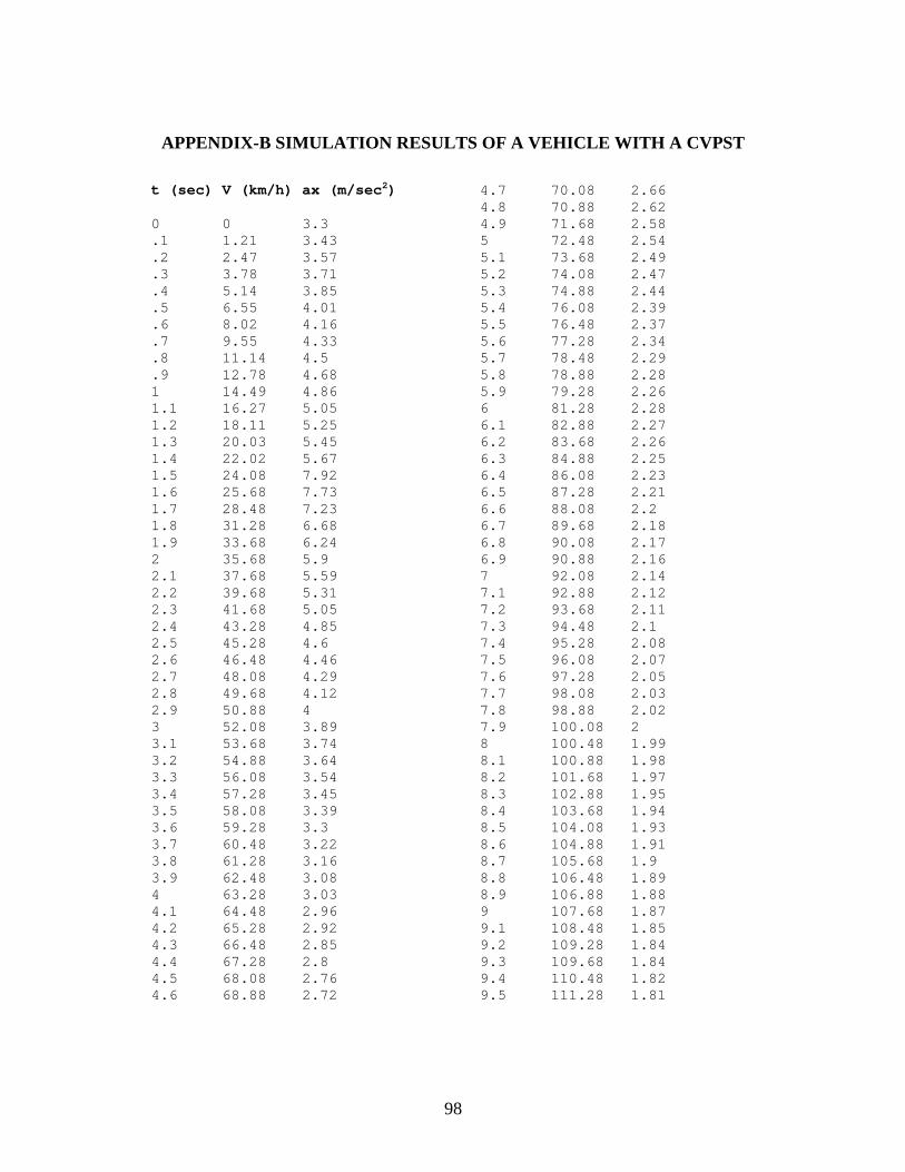
98
APPENDIX-B SIMULATION RESULTS OF A VEHICLE WITH A CVPST
t (sec) V (km/h) ax (m/sec2)
0 0 3.3.1 1.21 3.43.2 2.47 3.57.3 3.78 3.71.4 5.14 3.85.5 6.55 4.01.6 8.02 4.16.7 9.55 4.33.8 11.14 4.5.9 12.78 4.681 14.49 4.861.1 16.27 5.051.2 18.11 5.251.3 20.03 5.451.4 22.02 5.671.5 24.08 7.921.6 25.68 7.731.7 28.48 7.231.8 31.28 6.681.9 33.68 6.242 35.68 5.92.1 37.68 5.592.2 39.68 5.312.3 41.68 5.052.4 43.28 4.852.5 45.28 4.62.6 46.48 4.462.7 48.08 4.292.8 49.68 4.122.9 50.88 43 52.08 3.893.1 53.68 3.743.2 54.88 3.643.3 56.08 3.543.4 57.28 3.453.5 58.08 3.393.6 59.28 3.33.7 60.48 3.223.8 61.28 3.163.9 62.48 3.084 63.28 3.034.1 64.48 2.964.2 65.28 2.924.3 66.48 2.854.4 67.28 2.84.5 68.08 2.764.6 68.88 2.72
4.7 70.08 2.664.8 70.88 2.624.9 71.68 2.585 72.48 2.545.1 73.68 2.495.2 74.08 2.475.3 74.88 2.445.4 76.08 2.395.5 76.48 2.375.6 77.28 2.345.7 78.48 2.295.8 78.88 2.285.9 79.28 2.266 81.28 2.286.1 82.88 2.276.2 83.68 2.266.3 84.88 2.256.4 86.08 2.236.5 87.28 2.216.6 88.08 2.26.7 89.68 2.186.8 90.08 2.176.9 90.88 2.167 92.08 2.147.1 92.88 2.127.2 93.68 2.117.3 94.48 2.17.4 95.28 2.087.5 96.08 2.077.6 97.28 2.057.7 98.08 2.037.8 98.88 2.027.9 100.08 28 100.48 1.998.1 100.88 1.988.2 101.68 1.978.3 102.88 1.958.4 103.68 1.948.5 104.08 1.938.6 104.88 1.918.7 105.68 1.98.8 106.48 1.898.9 106.88 1.889 107.68 1.879.1 108.48 1.859.2 109.28 1.849.3 109.68 1.849.4 110.48 1.829.5 111.28 1.81
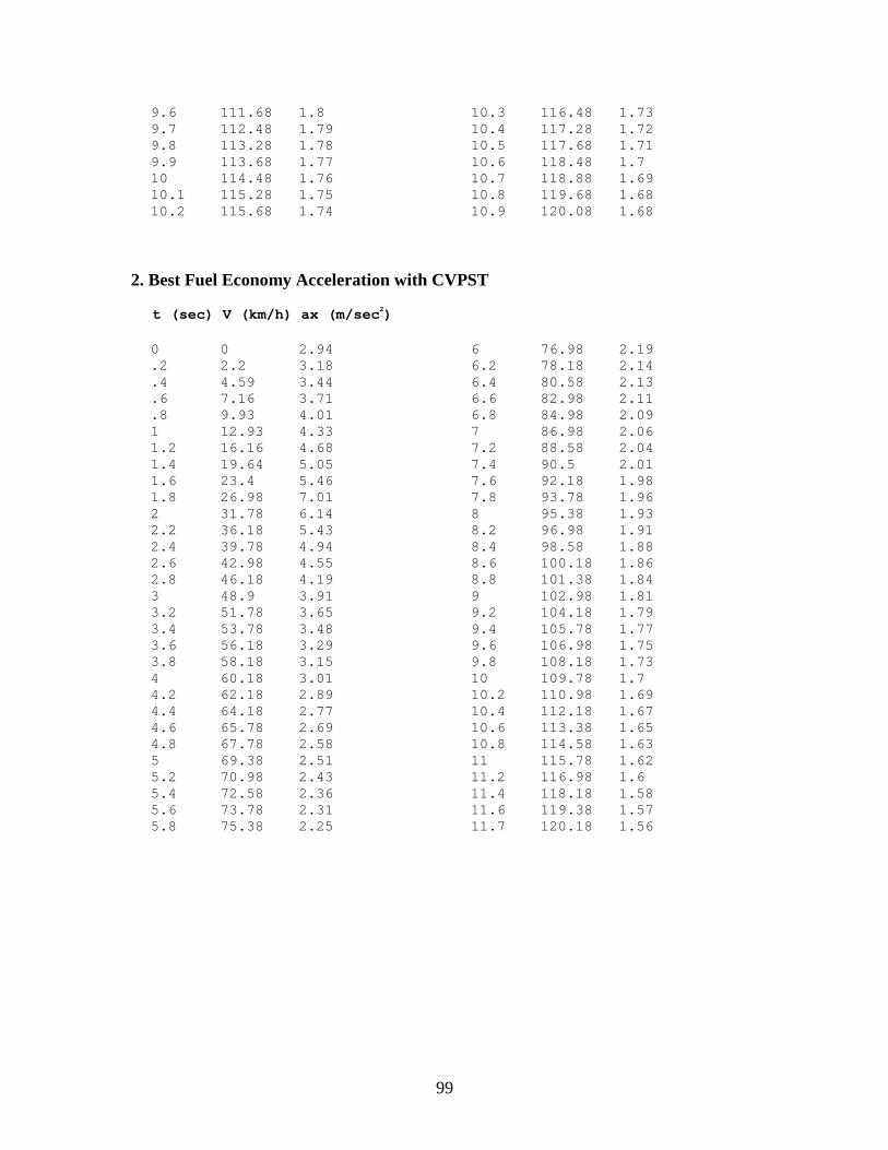
99
9.6 111.68 1.89.7 112.48 1.799.8 113.28 1.789.9 113.68 1.7710 114.48 1.7610.1 115.28 1.7510.2 115.68 1.74
10.3 116.48 1.7310.4 117.28 1.7210.5 117.68 1.7110.6 118.48 1.710.7 118.88 1.6910.8 119.68 1.6810.9 120.08 1.68
2. Best Fuel Economy Acceleration with CVPST
t (sec) V (km/h) ax (m/sec2)
0 0 2.94.2 2.2 3.18.4 4.59 3.44.6 7.16 3.71.8 9.93 4.011 12.93 4.331.2 16.16 4.681.4 19.64 5.051.6 23.4 5.461.8 26.98 7.012 31.78 6.142.2 36.18 5.432.4 39.78 4.942.6 42.98 4.552.8 46.18 4.193 48.9 3.913.2 51.78 3.653.4 53.78 3.483.6 56.18 3.293.8 58.18 3.154 60.18 3.014.2 62.18 2.894.4 64.18 2.774.6 65.78 2.694.8 67.78 2.585 69.38 2.515.2 70.98 2.435.4 72.58 2.365.6 73.78 2.315.8 75.38 2.25
6 76.98 2.196.2 78.18 2.146.4 80.58 2.136.6 82.98 2.116.8 84.98 2.097 86.98 2.067.2 88.58 2.047.4 90.5 2.017.6 92.18 1.987.8 93.78 1.968 95.38 1.938.2 96.98 1.918.4 98.58 1.888.6 100.18 1.868.8 101.38 1.849 102.98 1.819.2 104.18 1.799.4 105.78 1.779.6 106.98 1.759.8 108.18 1.7310 109.78 1.710.2 110.98 1.6910.4 112.18 1.6710.6 113.38 1.6510.8 114.58 1.6311 115.78 1.6211.2 116.98 1.611.4 118.18 1.5811.6 119.38 1.5711.7 120.18 1.56
100
VITA
Zhijian Lu was born on May 14, 1958 in Xian, Shaanxi, the People’s Republic of
China. He received his secondary education at Xian 63rd Middle and High School in his
hometown. He received his degree of Bachelor of Science in Mechanical Engineering
from Xian Mining Institute in January 1982. Mr. Lu started to work at Xian Design and
Research Institute in January 1982. He worked as a mechanical engineer from 1982 to
1992 and worked as a director and a senior engineer from 1993 to 1994.
Mr. Lu was a visiting scholar in West Virginia University from 1995 to 1997. In
the fall semester of 1996, he was admitted to the Engineering and Mineral Resources
Master of Science program at the Mechanical and Aerospace Engineering Department,
College of Engineering and Mineral Resources, West Virginia University, Morgantown,
West Virginia. Currently, he is a candidate of Master degree.
Zhijian married Shenglan Zhang in Xian, Shaanxi, China. They have a son named
Qing.
Top Related