


Languages
Pages
Legal


ABSTRACT
Title of Document: FLOW REGIME DRIVEN THERMAL ENHANCEMENT
IN INTERNALLY-GROOVED TUBES
Darin Sharar, Doctor of Philosophy, 2016.
Directed by: Professor Avram Bar-Cohen
Department of Mechanical Engineering
Internally-grooved refrigeration tubes maximize tube-side evaporative heat transfer
rates and have been identified as a most promising technology for integration into compact
cold plates. Unfortunately, the absence of phenomenological insights and physical models
hinders the extrapolation of grooved-tube performance to new applications. The success
of regime-based heat transfer correlations for smooth tubes has motivated the current effort
to explore the relationship between flow regimes and enhanced heat transfer in internally-
grooved tubes. In this thesis, a detailed analysis of smooth and internally-grooved tube
data reveals that performance improvement in internally-grooved tubes at low-to-
intermediate mass flux is a result of early flow regime transition. Based on this analysis, a
new flow regime map and corresponding heat transfer coefficient correlation, which
account for the increased wetted angle, turbulence, and Gregorig effects unique to
internally-grooved tubes, were developed.
A two-phase test facility was designed and fabricated to validate the newly-
developed flow regime map and regime-based heat transfer coefficient correlation. As part
of this setup, a non-intrusive optical technique was developed to study the dynamic nature
of two-phase flows. It was found that different flow regimes result in unique temporally

varying film thickness profiles. Using these profiles, quantitative flow regime
identification measures were developed, including the ability to explain and quantify the
more subtle transitions that exist between dominant flow regimes.
Flow regime data, based on the newly-developed method, and heat transfer
coefficient data, using infrared thermography, were collected for two-phase HFE-7100
flow in horizontal 2.62mm - 8.84mm diameter smooth and internally-grooved tubes with
mass fluxes from 25-300 kg/m²s, heat fluxes from 4-56 kW/m², and vapor qualities
approaching 1. In total, over 6500 combined data points for the adiabatic and diabatic
smooth and internally-grooved tubes were acquired.
Based on results from the experiments and a reinterpretation of data from
independent researchers, it was established that heat transfer enhancement in internally-
grooved tubes at low-to-intermediate mass flux is primarily due to early flow regime
transition to Annular flow. The regime-based heat transfer coefficient outperformed
empirical correlations from the literature, with mean and absolute deviations of 4.0% and
32% for the full range of data collected.

FLOW REGIME DRIVEN THERMAL ENHANCEMENT IN INTERNALLY-
GROOVED TUBES
By:
Darin James Sharar
Dissertation Submitted to the Faculty of the Graduate School of the
University of Maryland, College Park in partial fulfillment
of the requirements for the degree
of Doctor of Philosophy
2016
Advisory Committee:
Dr. Avram Bar-Cohen, Chair
Dr. Bongtae Han
Dr. Michael Ohadi
Dr. Patrick McCluskey
Dr. Mario Dagenais, Dean’s Representative

This work was supported by the U.S. Army Research Laboratory under Contract
W911QX-15-D-0023, Task 0001. The views and conclusions contained in this document
are those of the author, Darin J. Sharar, and should not be interpreted as presenting the
official policies or position, either expressed or implied, of the U.S. Government.

ii
Acknowledgements
I am most grateful to my advisor, Dr. Avram Bar-Cohen, for giving me the
opportunity and motivation to undertake this work. Dr. Bar-Cohen, it’s been an honor to
complete my PhD under your direction.
I would like to thank my Dissertation defense committee; Professor Michael Ohadi,
Professor Bongtae Han, Professor Patrick McCluskey, and Professor Mario Dagenais for
their advice and guidance through all stages of this work. I would like to give special
thanks to Dr. Arthur Bergles, whose guidance, insight, and support, as well as pioneering
work on two-phase enhancement, has inspired and informed much of this ongoing research
effort. He will be sorely missed, both professionally and personally.
Thanks to my colleagues at the Army Research Laboratory (ARL) and University
of Maryland (UMD) for their cooperation and friendship. Among them, special thanks to
Dr. Brian Morgan, Dr. Lauren Boteler, and Nicholas Jankowski for their constant support.
I also acknowledge my former and current lab-mates, working in collaboration with the
Maryland Embedded Cooling Center (MEmCo) and Thermal Management of Photonic and
Electronic Systems (TherPES) laboratory: Dr. Emil Rahim, Dr. Peng Wang, Dr. Juan
Cevallos, Dr. Mike Manno, Horacio Nochetto, Frank Robinson, Caleb Holloway, Alex
Reeser, and Michael Fish.
Finally, many thanks to my parents Susan and Joseph Sharar, my wife Kristen
Oursler Sharar, my sister Anne King, her husband Scott King, and their two beautiful
children Ryleigh and Grayson, my friends, and my extended family for their enduring love
and support. You mean the world to me.

iii
Table of Contents Acknowledgements ............................................................................................................. ii
Table of Contents ............................................................................................................... iii
List of Tables.. ................................................................................................................. viii
List of Figures. .................................................................................................................. xii
Chapter 1: Introduction ..................................................................................................1
1.1 Power Conversion Electronics - Thermal Issue .................................................. 2
1.2 Power Electronic Thermal Management ............................................................ 3
1.3 Two-Phase Surface Enhancements and Internally-Grooved Tubes .................... 6
1.4 Goals and Outline ............................................................................................. 10
1.4.1 Goals ..............................................................................................................10
1.4.2 Outline............................................................................................................11
Chapter 2: Two-Phase Flow Boiling Fundamentals ....................................................14
2.1 Diabatic Two-Phase Flow Patterns and Dependence on Heat Transfer ........... 14
2.2 Two-Phase Flow Pattern Maps ......................................................................... 17
2.3 Smooth Tube Regime-Based Heat Transfer Models ........................................ 21
Chapter 3: Fundamental Studies of Flow Patterns and Heat Transfer in Internally-
Grooved Tubes ...................................................................................................................24
3.1 Flow Regime Quantification ............................................................................. 25
3.2 Studies on Conventional Internally-Grooved Tubes ......................................... 25
3.2.1 Flow Regime Transition Mechanisms ...........................................................27
3.2.2 Halogenated Fluids at Standard Pressure and Temperature ..........................30
3.2.3 Refrigerant/Oil Mixtures ................................................................................40

iv
3.2.4 Halogenated Fluids and CO2 at Elevated Reduced Pressure .........................40
3.2.5 Geometric Considerations ..............................................................................43
3.3 Studies on Small Internally-Grooved Tubes ..................................................... 44
3.3.1 Refrigerant/Oil Mixtures ................................................................................46
3.3.2 Geometric Considerations ..............................................................................47
3.4 Flow Regime Maps and Regime-Inspired Heat Transfer Coefficient Correlations
for Internally-Grooved Tubes ....................................................................................... 47
3.5 Summary ........................................................................................................... 52
Chapter 4: New Flow Regime Map and Heat Transfer Coefficient Correlation for
Internally-Grooved Tubes ..................................................................................................57
4.1 Taitel-Dukler [46] Annular Transition Criteria ................................................ 57
4.2 Traditional Wojtan et al. [30] Flow Regime Map for Smooth Tubes ............... 60
4.3 Modified Sharar et al. [29] Flow Regime Map for Internally-Grooved Tubes 64
4.4 Traditional Wojtan et al. [31] Heat Transfer Coefficient Correlation .............. 66
4.5 Modified Heat Transfer Coefficient Correlation .............................................. 73
4.6 Model Simulation.............................................................................................. 75
4.7 Summary ........................................................................................................... 82
Chapter 5: Experimental Setup and Procedures ..........................................................84
5.1 Two-Phase Testing Setup ................................................................................. 84
5.2 Tube Heating Method ....................................................................................... 88
5.3 Fluid Selection .................................................................................................. 89
5.4 Experimental Ranges ........................................................................................ 91
5.5 Data Acquisition ............................................................................................... 93

v
5.6 Deduction of Vapor Quality.............................................................................. 94
5.7 Calculating Heat Transfer Coefficient .............................................................. 95
5.8 Uncertainty Analysis ......................................................................................... 98
Chapter 6: Total Internal Reflection Flow Regime Quantification ...........................102
6.1 Flow Regime Quantification Methods Available in the Literature ................ 103
6.2 Theory ............................................................................................................. 104
6.3 TIR Setup and Procedures .............................................................................. 107
6.3.1 Implementation of the TIR Technique .........................................................107
6.3.2 Experimental Ranges for Method Validation ..............................................108
6.3.3 Data Acquisition ..........................................................................................108
6.3.4 Data Reduction.............................................................................................109
6.4 Experimental Results ...................................................................................... 112
6.4.1 Accuracy of the Total Internal Reflection Technique ..................................112
6.4.2 Limitations of the Total Internal Reflection Technique during Two-Phase
Testing......................................................................................................................115
6.4.3 Characterization of Primary Flow Regimes .................................................117
6.4.4 Characterization of Sub-Regimes and Subtle Differences of Primary Flow
Regimes....................................................................................................................121
6.4.5 TIR Validation with Existing Flow Regime Maps ......................................125
6.5 Summary ......................................................................................................... 131
Chapter 7: Single-Phase Data and Discussion ...........................................................133
7.1 Single-Phase Energy Balance ......................................................................... 133

vi
7.2 Single-Phase Heat Transfer Measurements and Comparison to Smooth Tube
Correlations ................................................................................................................. 134
7.3 Single-Phase Heat Transfer Measurements and Comparison to Internally-
Grooved Tube Correlations......................................................................................... 137
Chapter 8: Two-Phase Data and Discussion ..............................................................142
8.1 8.84mm Smooth and Internally-Grooved Tubes ............................................ 143
8.1.1 Influence of Mass Flux and Flow Regime ...................................................143
8.1.2 Influence of Heat Flux .................................................................................149
8.2 4.54mm Smooth and Internally-Grooved Tubes ............................................ 153
8.2.1 Influence of Mass Flux and Flow Regime ...................................................153
8.2.2 Influence of Heat Flux .................................................................................159
8.3 2.8mm Smooth and 2.62mm Internally-Grooved Tubes ................................ 162
8.3.1 Influence of Mass Flux and Flow Regime ...................................................162
8.3.2 Influence of Heat Flux .................................................................................168
8.4 Tabulation of Flow Regime Modeling Results ............................................... 171
8.5 Enhancement Ratio ......................................................................................... 173
8.6 Statistical Assessment of the Heat Transfer Coefficient Correlations ............ 176
8.6.1 Smooth Tubes ..............................................................................................177
8.6.2 Internally-Grooved Tubes ............................................................................180
8.7 Comparison to Data from the Literature ......................................................... 186
8.7.1 Flow Regime Data .......................................................................................186
8.7.2 Heat Transfer Coefficient ............................................................................192
8.8 Applicability of the Sharar et al. Model.......................................................... 196

vii
8.9 Refitting the Sharar et al. Flow Regime Map ................................................. 198
8.10 Summary ......................................................................................................... 202
Chapter 9: Conclusions and Future Work .................................................................205
9.1 Conclusions ..................................................................................................... 205
9.2 Future Work .................................................................................................... 209
Appendix A Atomic Layer Deposition Tube Coating Method ....................................212
A.1 Candidate Heating Methods ............................................................................ 212
A.2 Atomic Layer Deposition Heating .................................................................. 213
A .2.1 ALD Uniformity ..........................................................................................214
A .2.2 Pinhole Defects in ALD ...............................................................................215
A .2.3 Ruthenium ALD...........................................................................................218
Appendix B Matlab Code for Total Internal Reflection ...............................................219
B.1 Preprocessing .................................................................................................. 221
B.2 Importing the Picture and Finding the Location of the First Fully Reflected
Ray….. ........................................................................................................................ 221
B.3 Determining the Number of Pixels Between Lines ........................................ 223
B.4 Defining Properties and Dimensions .............................................................. 227
B.5 TIR Film Thickness Calculation ..................................................................... 227
Appendix C 8.84mm Smooth and Internally-Grooved Tube Data ..............................229
Appendix D 4.54mm Smooth and Internally-Grooved Tube Data ..............................239
Appendix E 2.8mm Smooth and 2.62mm Internally-Grooved Tube Data ..................248
Appendix F Statistical Analysis of Heat Transfer Results ...........................................256
Chapter 10: Works Cited .............................................................................................267
viii
List of Tables
Table 1: Classification of flow boiling enhancement techniques ....................................... 7
Table 2: Geometric parameters and fin efficiencies for three Wieland copper internally-
grooved tubes ...................................................................................................................... 8
Table 3: Performance comparison of internally-grooved tubes to smooth tubes ............... 9
Table 4: Summary of relevant studies on flow patterns and heat transfer in macroscale
internally-grooved tubes ................................................................................................... 26
Table 5: Summary of relevant studies on flow patterns and heat transfer in small and
microscale internally-grooved tubes ................................................................................. 45
Table 6: Summary of relevant studies on new flow pattern maps for internally-grooved
tubes and regime-based heat transfer coefficient models ................................................. 48
Table 7: Comparison of fluids (and properties) used for empirically fitted flow regime maps
and candidate fluids .......................................................................................................... 91
Table 8: Geometric parameters of internally-grooved and smooth tubes for the current
study .................................................................................................................................. 92
Table 9: Heat transfer coefficients applied at different axially and circumferentially
varying locations for the ANSYS numerical model ......................................................... 98
Table 10: Summary of uncertainties for sensors and parameters .................................. 101
Table 11: Comparison of thickness prediction using test setup and Matlab algorithm to
actual thickness values .................................................................................................... 115
Table 12: Geometric properties and maximum measurable film thickness for different
operating conditions ........................................................................................................ 117

ix
Table 13: Statistical analysis of the experimental single-phase smooth tube heat transfer
measurements .................................................................................................................. 137
Table 14: Statistical analysis of the experimental single-phase internally-grooved tube heat
transfer measurements .................................................................................................... 139
Table 15: Predictive accuracy of Traditional Wojtan et al. [30] flow regime map for the
smooth tube data ............................................................................................................. 172
Table 16: Predictive accuracy of Traditional Wojtan et al. [30] and Modified Sharar et al.
[29] flow regime maps for the internally-grooved tube data ......................................... 173
Table 17: Predictive accuracy of two-phase smooth tube heat transfer coefficient
correlations from Wojtan et al. [31], Chen [56], Shah [57], Kandlikar [93], and Gungor-
Winterton [59] [60] ......................................................................................................... 180
Table 18: Predictive accuracy of Modified Sharar and Bar-Cohen two-phase internally-
grooved tube heat transfer coefficient correlation and correlations from Thome et al. [91],
Cavallini et al. [117], Chamra and Mago [162], Wu et al. [103], and Yun et al. [90] .... 182
Table 19: Predictive accuracy of Traditional Wojtan et al. [30] and Modified Sharar et al.
[29] flow regime maps .................................................................................................... 192
Table 20: Saturated Properties of Various Fluids .......................................................... 198
Table 21: Material properties of interest for ALD coated copper tubes ......................... 214
Table 22: Predictive accuracy of two-phase smooth tube heat transfer coefficient
correlations from Wojtan et al. [31], Chen [56], Shah [57], Kandlikar [93], and Gungor-
Winterton [59] [60] ......................................................................................................... 264

x
Table 23: Predictive accuracy of two-phase smooth tube heat transfer coefficient
correlations from Wojtan et al. [31], Chen [56], Shah [57], Kandlikar [93], and Gungor-
Winterton [59] [60] ......................................................................................................... 264
Table 24: Predictive accuracy of two-phase smooth tube heat transfer coefficient
correlations from Wojtan et al. [31], Chen [56], Shah [57], Kandlikar [93], and Gungor-
Winterton [59] [60] ......................................................................................................... 264
Table 25: Summary of the predictive accuracy of two-phase smooth tube heat transfer
coefficient correlations from Wojtan et al. [31], Chen [56], Shah [57], Kandlikar [93], and
Gungor-Winterton [59] [60] to the 2.8mm to 8.84mm experimental results.................. 265
Table 26: Predictive accuracy of the Modified Sharar and Bar-Cohen internally-grooved
tube correlation, and correlations from Thome et al. [91], Cavallini et al. [117], Chamra
and Mago [162], Wu et al. [103], and Yun et al. [90] compared to the 8.84mm experimental
results .............................................................................................................................. 265
Table 27: Predictive accuracy of the Modified Sharar and Bar-Cohen internally-grooved
tube correlation, and correlations from Thome et al. [91], Cavallini et al. [117], Chamra
and Mago [162], Wu et al. [103], and Yun et al. [90] compared to the 4.54mm experimental
results .............................................................................................................................. 265
Table 28: Predictive accuracy of the Modified Sharar and Bar-Cohen internally-grooved
tube correlation, and correlations from Thome et al. [91], Cavallini et al. [117], Chamra
and Mago [162], Wu et al. [103], and Yun et al. [90] compared to the 2.62mm experimental
results .............................................................................................................................. 266
Table 29: Summary of the predictive accuracy of the Modified Sharar and Bar-Cohen
internally-grooved tube correlation, and correlations from Thome et al. [91], Cavallini et

xi
al. [117], Chamra and Mago [162], Wu et al. [103], and Yun et al. [90] for the 2.62mm to
8.84mm experimental results .......................................................................................... 266

xii
List of Figures
Figure 1: Midsize hybrid electric power requirements (adapted from [1]) ....................... 2
Figure 2: Dissipated heat vs flow rate for water using latent heat and sensible heat ........ 6
Figure 3: a) Schematic of internally-grooved tube (adapted from [23]) and b) photograph
of a 9.52 mm Wieland internally-grooved tube (adapted from [22]) ................................. 8
Figure 4: a) Schematic of flow patterns and b) the corresponding heat transfer mechanisms
and qualitative variation of the heat transfer coefficients for flow boiling in a horizontal
tube (adapted from [34]) ................................................................................................... 15
Figure 5: a) Taitel-Dukler [46] adiabatic flow regime map and b) Wojtan et al. [30] diabatic
flow regime map for evaporation of R134a at -15ºC in a 9mm smooth tube with a heat flux
of 4 kW/m² ........................................................................................................................ 19
Figure 6: Comparison of experimental heat transfer data (adapted from Filho and Jabardo
[38]) (hollow data points) for R134a at 5ºC in an 8.92 mm smooth tube with a heat flux of
5 kW/m² to a) the Wojtan et al. heat transfer model [31] and b) Wojtan et al. flow regime
map [30] ............................................................................................................................ 22
Figure 7: Film thickness profiles for smooth (dashed lines) and 18° internally-grooved
(solid red lines) tubes with 15.1 mm ID and mass fluxes of a) G=44 kg/m²s and x=0.6 and
b) G=120 kg/m²s and x=0.76 [27], plotted on the simplified Wojtan et al. [30] flow regime
map .................................................................................................................................... 29
Figure 8: Experimental flow visualization results from Yu et al. [66] for R134a at 6ºC with
a heat flux of 20 kW/m² plotted on a simplified Wojtan et al. [30] map for a) 10.7 mm ID
smooth tube and b) 11.1 mm ID internally-grooved tube ................................................. 31
xiii
Figure 9: a) Heat transfer coefficient vs vapor quality and b) accompanying enhancement
factor from several researchers with low mass flux (100 – 163 kg/m²s) .......................... 32
Figure 10: a) Heat transfer coefficient vs vapor quality and b) accompanying enhancement
factor from several researchers with high mass flux (300 - 326 kg/m²s) ......................... 33
Figure 11: Experimental flow visualization results of Filho and Barbieri [75] for R134a at
5ºC in an 8.92 mm smooth and internally-grooved tube with a heat flux of 5 kW/m² plotted
on a simplified Wojtan et al. [30] flow regime map ......................................................... 35
Figure 12: Flow visualization results from Colombo et al. [79] for 8.92 mm ID a) smooth
and b) internally-grooved tubes with R134a at 5ºC and a heat flux of 4.2 kW/m² plotted on
the Wojtan et al. [30] flow regime map ............................................................................ 37
Figure 13: Experimental flow visualization results from Spindler and Müller-Steinhagen
[74] for a) R134a and b) R404A at -20ºC with a heat flux of 7.5 kW/m² in one 8.92 mm ID
internally-grooved tube plotted on a corresponding Wojtan et al. [30] flow regime map 40
Figure 14: Experimental flow visualization results from Schael and Kind [70] for CO2
flow boiling in an 8.92 mm ID internally-grooved tube with heat fluxes up to 120 kW/m²
at reduced pressures of a) 0.54 (Tsat = 5°C) and b) 0.36 (Tsat = -10°C) plotted on the
Mastrullo et al. [54] flow regime map .............................................................................. 42
Figure 15: Generalized transition boundaries in Taitel-Dukler model (adapted from [46])
........................................................................................................................................... 58
Figure 16: Traditional smooth tube Wojtan et al. [30] diabatic flow regime map for
evaporation of R134a at -15ºC in a 9mm smooth tube with a heat flux of 4 kW/m² ....... 60
Figure 17: Two-phase Stratified flow cross-section (adapted from [30])........................ 61

xiv
Figure 18: a) Traditional smooth tube Wojtan et al. [30] and b) modified Sharar et al. [29]
internally-grooved tube diabatic flow regime map for evaporation of R134a at -15ºC in
9mm tubes with a heat flux of 4 kW/m² ........................................................................... 66
Figure 19: Modeling simulation results for a) original Wojtan et al. [30] flow regime map
and b) associated heat transfer coefficient [31] in an 8.84mm smooth tube with HFE-7100
at 61°C and a heat flux of 4 kW/m² .................................................................................. 77
Figure 20: Modeling simulation results for a) Modified Sharar et al. [29] internally-
grooved tube flow regime map and b) associated heat transfer coefficient in an 8.84mm
internally-grooved tube with HFE-7100 at 61°C and a heat flux of 4 kW/m² .................. 78
Figure 21: Simulated results comparing enhancement ratio vs mass flux for 8.84mm
smooth and internally-grooved tubes with HFE-7100 at 61°C and a heat flux of 4 kW/m²
as shown in Figure 19 and Figure 20 ................................................................................ 80
Figure 22: Simulated results comparing enhancement ratio, Emf, and Erb vs mass flux for
8.84mm smooth and internally-grooved tubes with HFE-7100 at 61°C and a heat flux of 4
kW/m² ............................................................................................................................... 82
Figure 23: Schematic of two-phase flow test setup: a) reservoir and degasser b) Fluid-o-
Tech pump c) Atrato or Kobold flow meter d) control valves e) inline heater f) 0.2m
developing flow section g) 0.2m test tube h) 8cm sight glass (location of high speed flow
visualization and TIR method) i) condenser P) pressure transducers and T) thermocouple
probes DP) differential pressure transducer ...................................................................... 85
Figure 24: Schematic of custom IR mirror setup for measuring temperature on the top,
middle, and side of the test section ................................................................................... 87

xv
Figure 25: Schematic of custom IR mirror setup for measuring temperature on the top,
middle, and side of the test section, and an IR photograph of the 2.80mm smooth tube
during testing .................................................................................................................... 88
Figure 26: Photograph of a smooth tube coated with a thin-film heater ......................... 89
Figure 27: Schematic of 1-D radial heat conduction in the Parylene-C/Ti-Pt coated tubes
........................................................................................................................................... 96
Figure 28: Numerical results for a circumferentially and axially varying heat transfer
coefficient ......................................................................................................................... 97
Figure 29: Principle of Total Internal Reflection (TIR) film thickness measurement
technique ......................................................................................................................... 104
Figure 30: Two-phase flow regimes (bottom) and associated film thickness profiles (top)
......................................................................................................................................... 106
Figure 31: a) Raw image of reflected light ring on a glass tube with no film thickness, b)
Image after converting to black and white and contrast enhancement, and c) Image after
converting to binary ........................................................................................................ 112
Figure 32: Binary images of validation samples a) 0 μm film, b) 183 μm film, c) 449 μm
film, and d) 1005 μm film ............................................................................................... 114
Figure 33: Schematic of the maximum measurable film thickness (adapted from [154])
......................................................................................................................................... 116
Figure 34: Unique temporally varying two-phase film thickness profiles in an 8.84 mm ID
smooth tube for a ‘Flooded’ condition (230 kg/m²s), ‘Stratified’ condition (15 kg/m²s,
x=0.067), ‘Intermittent’ condition (230 kg/m²s, x=0.01), and ‘Annular’ condition (120
kg/m²s, x>0.15) ............................................................................................................... 118

xvi
Figure 35: Photographs of high speed flow visualization .............................................. 119
Figure 36: Intermittent flow film thickness profiles for a) 15 kg/m²s and x=0.004 and b)
230 kg/m²s and x=0.023.................................................................................................. 122
Figure 37: Film thickness profile for intermediate Slug-Annular flow with a) 60 kg/m²s
and x=0.014 and b) 60 kg/m²s and x=0.066 ................................................................... 124
Figure 38: Two-Phase flow regime data plotted on a) Taitel-Dukler [46] map, b) Ullmann-
Brauner [141] map, and c) Wojtan et al. [30] map ......................................................... 127
Figure 39: Single-phase liquid energy balance ratio for HFE-7100 in different tube
diameters ......................................................................................................................... 134
Figure 40: Experimental and predicted single-phase heat transfer coefficient vs mass flux
for a) 8.84 mm smooth tube, b) 4.54 mm smooth tube, and c) 2.8 mm smooth tube ..... 136
Figure 41: Experimental and predicted single-phase heat transfer coefficient vs mass flux
for a) 8.84 mm internally-grooved tube, b) 4.54 mm internally-grooved tube, and c) 2.62
mm internally-grooved tube ............................................................................................ 140
Figure 42: 8.84mm smooth tube data plotted on a) the Wojtan et al. [30] map and 8.84mm
internally-grooved tube data plotted on b) the Wojtan et al. [30] map and c) the Sharar et
al. [29] map with HFE-7100 at 61°C, G=50 kg/m²s, and q”=9 kW/m² .......................... 144
Figure 43: Comparison of heat transfer coefficient vs vapor quality for a mass flux of a)
25 kg/m²s, b) 75 kg/m²s, and c) 200 kg/m²s with HFE-7100 at 61°C and q”=9 kW/m² in
the 8.84mm tubes ............................................................................................................ 148
Figure 44: Comparison of heat transfer coefficient vs vapor quality for the 8.84mm tubes
with HFE-7100 at 61°C and a mass flux of 200 kg/m²s for heat fluxes of a) 4 kW/m², b) 9
kW/m², c) 18 kW/m², d) 28 kW/m², e) 40 kW/m², and f) 56 kW/m².............................. 151

xvii
Figure 45: 4.54mm smooth tube data plotted on a) the Wojtan et al. [30] map and 4.54mm
internally-grooved tube data plotted on b) the Wojtan et al. [30] map and c) the Sharar et
al. [29] map with HFE-7100 at 61°C, G=50 kg/m²s, and q”=9 kW/m² .......................... 154
Figure 46: Comparison of heat transfer coefficient vs vapor quality for a mass flux of a)
50 kg/m²s, b) 75 kg/m²s, and c) 200 kg/m²s with HFE-7100 at 61°C and q”=9 kW/m² in
the 4.54mm tubes ............................................................................................................ 157
Figure 47: Comparison of heat transfer coefficient vs vapor quality for the 4.54mm tubes
with HFE-7100 at 61°C and a mass flux of 200 kg/m²s for heat fluxes of a) 4 kW/m², b) 9
kW/m², c) 18 kW/m², d) 28 kW/m², e) 40 kW/m², and f) 56 kW/m².............................. 160
Figure 48: 2.8mm smooth tube data plotted on a) the Wojtan et al. [30] map and 2.62mm
internally-grooved tube data plotted on b) the Wojtan et al. [30] map and c) the Sharar et
al. [29] map with HFE-7100 at 61°C, G=50 kg/m²s, and q”=9 kW/m² .......................... 164
Figure 49: Comparison of heat transfer coefficient vs vapor quality for a mass flux of a)
75 kg/m²s and b) 200 kg/m²s with HFE-7100 at 61°C and q”=9 kW/m² in 2.62-2.8mm
tubes ................................................................................................................................ 166
Figure 50: Comparison of heat transfer coefficient vs vapor quality for the 2.62-2.8mm
tubes with HFE-7100 at 61°C and a mass flux of 200 kg/m²s for heat fluxes of a) 4 kW/m²,
b) 9 kW/m², c) 18 kW/m², d) 28 kW/m², e) 40 kW/m², and f) 56 kW/m² ...................... 170
Figure 51: Enhancement ratio vs mass flux with current data for the 8.84mm, 4.54mm,
and 2.62mm internally-grooved tubes ............................................................................ 174
Figure 52: Comparison of the 8.84mm smooth tube experimental data for HFE-7100 at
61°C with correlations from a) Wojtan et al. [31], b) Chen [56], c) Shah [57], d) Kandlikar
[93], e) Gungor-Winterton ‘original’ [59], and f) Gungor-Winterton ‘new’ [60] .......... 178

xviii
Figure 53: Comparison of the 8.84mm internally-grooved tube experimental data for HFE-
7100 at 61°C with a) the Modified Sharar and Bar-Cohen correlation and correlations from
b) Thome et al. [91], c) Cavallini et al. [117], d) Chamra and Mago [162], e) Wu et al.
[103], and f) Yun et al. [90] ............................................................................................ 181
Figure 54: Example of heat transfer coefficient uncertainty and deviation near the
transition boundary between Stratified-Wavy and Annular flow for HFE-7100 at 61°C in
the 8.84mm tubes; a) locus of different flowrates on the Modified flow regime map and b)
resulting heat transfer coefficients .................................................................................. 184
Figure 55: 11.1 mm ID internally-grooved tube experimental flow visualization results
from Yu et al. [66] for R134a at 6ºC with a heat flux of 20 kW/m² plotted on the a) original
Wojtan et al. [30] map and b) Modified Sharar et al. [29] map ...................................... 187
Figure 56: 8.92 mm ID internally-grooved tube experimental flow visualization results
from Colombo et al. [79] with R134a at 5ºC and a heat flux of 4.2 kW/m² plotted on the a)
original Wojtan et al. [30] map and b) Modified Sharar et al. [29] map ........................ 189
Figure 57: 8.92 mm ID internally-grooved tube experimental flow visualization results
from Spindler and Müller-Steinhagen [74] for R134a at -20ºC with a heat flux of 7.5 kW/m²
plotted on the a) original Wojtan et al. [30] map and b) Modified Sharar et al. [29] map
......................................................................................................................................... 190
Figure 58: 8.92 mm ID internally-grooved tube experimental flow visualization results
from Spindler and Müller-Steinhagen [74] for R404a at -20ºC with a heat flux of 7.5 kW/m²
plotted on the a) original Wojtan et al. [30] map and b) Modified Sharar et al. [29] map
......................................................................................................................................... 191

xix
Figure 59: Heat transfer coefficient vs vapor quality for the original Wojtan et al. [31]
model, Modified heat transfer coefficient described in this Dissertation, and data from Yu
et al. [66] for an 11.1 mm smooth and internally-grooved tube with R134a at 6ºC and a
heat flux of 20 kW/m² ..................................................................................................... 193
Figure 60: Normalized enhancement ratio vs mass flux with data from the current study
and data from three independent researchers .................................................................. 195
Figure 61: 4.54mm internally-grooved tube data plotted on a) the Sharar et al. map [29]
described in Chapter 4 and b) the adjusted map based on the current data set with HFE-
7100 at 61°C, G=50 kg/m²s, and q”=9 kW/m² ............................................................... 199
Figure 62: Comparison of heat transfer coefficient vs vapor quality for a mass flux of 50
kg/m²s with HFE-7100 at 61°C and q”=9 kW/m² in the 4.54mm tubes superimposed with
a) heat transfer coefficient based on Sharar et al. [29] map and b) adjusted Sharar et al. map
......................................................................................................................................... 200
Figure 63: Schematic (side view) of the cantilever test setup made to test material thickness
in the ALD tool ............................................................................................................... 215
Figure 64: Schematic showing a copper metallic bump formed at a defect site when
electroplating a conductive substrate in an electrolytic solution of H2SO4 and CuSO4
(adapted from [165]) ....................................................................................................... 216
Figure 65: Comparison between SEM images of 200nm thick Alumina deposited on Cu-
coated Si substrates a) before and b) after electroplating process .................................. 217
Figure 66: SEM image of Ruthenium nucleation sites .................................................. 218

xx
Figure 67: a) Raw image of reflected light ring on a glass tube with no film thickness, b)
Image after converting to black and white and contrast enhancement, and c) Image after
converting to binary ........................................................................................................ 220
Figure 68: Heat transfer coefficient vs vapor quality for 8.84 mm ID smooth and internally-
grooved tubes at a mass flux of 300 kg/m²s and different heat fluxes ............................ 230
Figure 69: Heat transfer coefficient vs vapor quality for 8.84 mm ID smooth and internally-
grooved tubes at a mass flux of 200 kg/m²s and different heat fluxes ............................ 231
Figure 70: Heat transfer coefficient vs vapor quality for 8.84 mm ID smooth and internally-
grooved tubes at a mass flux of 175 kg/m²s and different heat fluxes ............................ 232
Figure 71: Heat transfer coefficient vs vapor quality for 8.84 mm ID smooth and internally-
grooved tubes at a mass flux of 150 kg/m²s and different heat fluxes ............................ 233
Figure 72: Heat transfer coefficient vs vapor quality for 8.84 mm ID smooth and internally-
grooved tubes at a mass flux of 125 kg/m²s and different heat fluxes ............................ 234
Figure 73: Heat transfer coefficient vs vapor quality for 8.84 mm ID smooth and internally-
grooved tubes at a mass flux of 100 kg/m²s and different heat fluxes ............................ 235
Figure 74: Heat transfer coefficient vs vapor quality for 8.84 mm ID smooth and internally-
grooved tubes at a mass flux of 75 kg/m²s and different heat fluxes .............................. 236
Figure 75: Heat transfer coefficient vs vapor quality for 8.84 mm ID smooth and internally-
grooved tubes at a mass flux of 50 kg/m²s and different heat fluxes .............................. 237
Figure 76: Heat transfer coefficient vs vapor quality for 8.84 mm ID smooth and internally-
grooved tubes at a mass flux of 25 kg/m²s and different heat fluxes .............................. 238
Figure 77: Heat transfer coefficient vs vapor quality for 4.54 mm ID smooth and internally-
grooved tubes at a mass flux of 300 kg/m²s and different heat fluxes ............................ 240

xxi
Figure 78: Heat transfer coefficient vs vapor quality for 4.54 mm ID smooth and internally-
grooved tubes at a mass flux of 200 kg/m²s and different heat fluxes ............................ 241
Figure 79: Heat transfer coefficient vs vapor quality for 4.54 mm ID smooth and internally-
grooved tubes at a mass flux of 175 kg/m²s and different heat fluxes ............................ 242
Figure 80: Heat transfer coefficient vs vapor quality for 4.54 mm ID smooth and internally-
grooved tubes at a mass flux of 150 kg/m²s and different heat fluxes ............................ 243
Figure 81: Heat transfer coefficient vs vapor quality for 4.54 mm ID smooth and internally-
grooved tubes at a mass flux of 125 kg/m²s and different heat fluxes ............................ 244
Figure 82: Heat transfer coefficient vs vapor quality for 4.54 mm ID smooth and internally-
grooved tubes at a mass flux of 100 kg/m²s and different heat fluxes ............................ 245
Figure 83: Heat transfer coefficient vs vapor quality for 4.54 mm ID smooth and internally-
grooved tubes at a mass flux of 75 kg/m²s and different heat fluxes .............................. 246
Figure 84: Heat transfer coefficient vs vapor quality for 4.54 mm ID smooth and internally-
grooved tubes at a mass flux of 50 kg/m²s and different heat fluxes .............................. 247
Figure 85: Heat transfer coefficient vs vapor quality for 2.8 mm ID smooth and 2.62 mm
ID internally-grooved tubes at a mass flux of 300 kg/m²s and different heat fluxes ...... 249
Figure 86: Heat transfer coefficient vs vapor quality for 2.8 mm ID smooth and 2.62 mm
ID internally-grooved tubes at a mass flux of 200 kg/m²s and different heat fluxes ...... 250
Figure 87: Heat transfer coefficient vs vapor quality for 2.8 mm ID smooth and 2.62 mm
ID internally-grooved tubes at a mass flux of 175 kg/m²s and different heat fluxes ...... 251
Figure 88: Heat transfer coefficient vs vapor quality for 2.8 mm ID smooth and 2.62 mm
ID internally-grooved tubes at a mass flux of 150 kg/m²s and different heat fluxes ...... 252
xxii
Figure 89: Heat transfer coefficient vs vapor quality for 2.8 mm ID smooth and 2.62 mm
ID internally-grooved tubes at a mass flux of 125 kg/m²s and different heat fluxes ...... 253
Figure 90: Heat transfer coefficient vs vapor quality for 2.8 mm ID smooth and 2.62 mm
ID internally-grooved tubes at a mass flux of 100 kg/m²s and different heat fluxes ...... 254
Figure 91: Heat transfer coefficient vs vapor quality for 2.8 mm ID smooth and 2.62 mm
ID internally-grooved tubes at a mass flux of 75 kg/m²s and different heat fluxes ........ 255
Figure 92: Comparison of the 8.84mm smooth tube experimental data for HFE-7100 at
61°C with a) Wojtan et al. [31], b) Chen [56], c) Shah [57], d) Kandlikar [93], e) Gungor-
Winterton ‘original’ [59], and f) Gungor-Winterton ‘new’ [60] .................................... 258
Figure 93: Comparison of the 4.54mm smooth tube experimental data for HFE-7100 at
61°C with a) Wojtan et al. [31], b) Chen [56], c) Shah [57], d) Kandlikar [93], e) Gungor-
Winterton ‘original’ [59], and f) Gungor-Winterton ‘new’ [60] .................................... 259
Figure 94: Comparison of the 2.8mm smooth tube experimental data for HFE-7100 at
61°C with a) Wojtan et al. [31], b) Chen [56], c) Shah [57], d) Kandlikar [93], e) Gungor-
Winterton ‘original’ [59], and f) Gungor-Winterton ‘new’ [60] .................................... 260
Figure 95: Comparison of the 8.84mm internally-grooved tube experimental data for HFE-
7100 at 61°C with a) the Modified Sharar and Bar-Cohen correlation, and correlations from
b) Thome et al. [91], c) Cavallini et al. [117], d) Chamra and Mago [162], e) Wu et al.
[103], and f) Yun et al. [90] ............................................................................................ 261
Figure 96: Comparison of the 4.54mm internally-grooved tube experimental data for HFE-
7100 at 61°C with a) the Modified Sharar and Bar-Cohen correlation, and correlations from
b) Thome et al. [91], c) Cavallini et al. [117], d) Chamra and Mago [162], e) Wu et al.
[103], and f) Yun et al. [90] ............................................................................................ 262

xxiii
Figure 97: Comparison of the 2.62mm internally-grooved tube experimental data for HFE-
7100 at 61°C with a) the Modified Sharar and Bar-Cohen correlation, and correlations from
b) Thome et al. [91], c) Cavallini et al. [117], d) Chamra and Mago [162], e) Wu et al.
[103], and f) Yun et al. [90] ............................................................................................ 263

1
Chapter 1: Introduction
The last several decades have witnessed a dramatic increase in the use of electronics
on a variety of transportation systems. This trend continues today in hybrid electric vehicle
(HEV), electric vehicle (EV), and plug-in hybrid electric vehicle (PHEV) technologies for
commercial and military applications. Military use can include both direct vehicle
applications, such as propulsion, and indirect applications such as electrically operated
arms or interfacing the vehicle electrical system to create a military base microgrid [1].
There are several motivations for replacing the traditional internal combustion (IC)
motors and mechanical drives with HEV equivalents on military platforms. One of the
most important reasons is the high cost of fuel. Transporting fuel to the theater through
dangerous routes and over long distances to geographically dispersed troops can
significantly increase the cost of fuel. The cost can rise from a commercial pump price of
several dollars per gallon to about $400/gal in the battlefield. If an airlift is needed, the
cost can reach $1000 per gallon [2]. As such, even a modest saving in fuel efficiency can
lead to huge cost savings for the Department of Defense.
HEV platforms also promise reduced operation noise and, as a result, improve
stealth capabilities and personnel safety in dangerous environments. Furthermore, HEVs
can be designed with one motor per axle or even hub motors in each of the wheels for
propulsion. This provides system redundancy, so that if one of the motors fails the vehicle
can operate in a degraded mode to reach a safe or serviceable location. An indirect benefit
of HEVs for military applications is the ability to interconnect multiple HEVs to provide
utility-level power to bases and other infrastructures in combat zones. With appropriate

2
control electronics, several HEVs can form a ‘micro-grid’ with a robust source of utility
power [1]. This use of HEVs can reduce the need for ancillary generators and power units,
therefore leading to savings stemming from acquisition and transportation costs.
1.1 Power Conversion Electronics - Thermal Issue
Figure 1 illustrates the continuous power needs for current commercial midsize
HEVs, full EVs, and PHEVs. As shown, continuous power demands increase through the
transition from commercial HEVs to PHEVs and all-electric drive applications such as fuel
cells or EVs. In the case of HEVs and PHEVs, electrical power requirements approach 30
to 60kW while the all-electric platforms reach 100kW for short durations.
Figure 1: Midsize hybrid electric power requirements (adapted from [1])
Power conversion electronics are a ubiquitous and enabling technology for the
success of current and future electric vehicle architectures; this is due to the disparate
Continuous
Mo
tori
ng
PH
EV
HE
V
All-Electric
Blended
Ele
ctri
c P
ow
er R
equ
irem
ent
(kW
)
Power Duration (s)

3
electrical systems common to these programs and the need to draw from a platform’s
single-voltage electrical bus. This mainly involves the use of power semiconductor
switches such as power diodes, metal oxide field effect transistors (MOSFETs), and
insulated gate bipolar transistors (IGBTs). Unfortunately, such electronic energy
conversion devices cannot be 100% efficient and vehicle systems requiring 100kW of
electrical power would have thermal losses of 2 to 4 kW, even with power electronic
conversion efficiencies of 96-98%. Larger systems or systems with multiple powertrain
motors, high-power bidirectional DC-DC converters, and power electronics modules could
have significantly higher waste heat challenges [1].
Aligned efforts aimed towards increasing total power while simultaneously
decreasing the component size and weight [3] have led to improvements in cost and power
density. However, increased power density has inevitably increased power electronic heat
flux and is presenting thermal management challenges for current and future systems; fast,
compact, IGBT devices can be expected to dissipate heat fluxes in upwards of 250 W/cm²
[1]. The primary target for thermal management of Silicon power electronics is sustained
operation below the maximum allowable temperature of 125˚C, since lower die
temperatures result in lower losses and better electrical performance. As such, efficient
thermal management of power electronics modules is critical to maintaining system-level
operational specifications without undermining efforts to improve power electronic size,
cost, weight, and power density.
1.2 Power Electronic Thermal Management
Traditionally, power electronics have relied on air-cooled heat sinks or liquid-
cooled cold plates to manage electronic waste heat, however new power-dense electronic

4
systems are further increasing waste heat and presenting challenges to the capabilities of
conventional cooling systems. The effect of higher heat flux electronics for air-cooled
systems is larger, heavier, costlier heat sinks and fans to compensate for insufficient
convective performance. The effect is equally dramatic with single-phase liquid cooling,
with higher heat fluxes requiring larger coolant flow rates to sufficiently cool the system
devices [4]. These large flow rates and subsequent pumping powers result in increasingly
bulky, heavy systems that consume more fuel [5] and undermine the current and future
efforts to reduce system cost and improve efficiency. Thus, there is a drive to develop
improved cooling components that are smaller and lighter, and have increased performance
relative to conventional liquid cold plates.
Cooling schemes using liquid-vapor phase change (two-phase cooling) have been
examined as a practical and cost-conscious next step beyond single-phase cooling. A two-
phase cooling system has several potential benefits over a standard single-phase liquid
cooling approach. First, the latent heat of vaporization for a particular fluid, reflecting the
heat absorbed to evaporate a unit mass, can be two orders of magnitude larger than the
specific (sensible) heat used in single-phase liquid cooling [6]. Therefore, evaporative
cooling provides the possibility of increased heat absorption per unit mass and volume of
fluid and improved heat acquisition effectiveness. The single-phase heat dissipation
relationship for water can be expressed as:
q = mCpdT = m × 4,186 × 1 = 4,186m (1)
where q is the heat dissipation, m is the mass flow rate, Cp is the specific heat of the fluid
(4186 kJ/kgK for water), and ∆T is the temperature rise of the fluid. Equation (1) assumes
an allowable fluid temperature rise of 1ºC, such that the heat dissipation can be expressed

5
as the product of mass flow rate and a constant. Similarly, the two-phase latent heat
dissipation relationship for water can be expressed as:
q = mhlgx = m × 2,257,000 × 1 = 2,257,000m (2)
where q is the heat dissipation, x is the quality (fraction of the mass flow rate that has been
vaporized), m is the mass flow rate, and hlg is the latent heat of vaporization of the fluid
(2,257 kJ/kg for water). Assuming full vaporization of the fluid (x=1.0), this heat
dissipation can also be expressed as the product of the flow rate and a constant.
As shown symbolically in Equation (1) and Equation (2), and graphically in Figure
2, the increased heat acquisition effectiveness of two-phase flow translates into lower flow
rates compared to single-phase flow for comparable heat dissipation. The potential benefit
of lower flow rates includes: smaller fluid reservoirs; smaller onboard fluid volume;
reduction in pumping power; smaller pumps; and a reduction in system weight and volume.
Additionally, two-phase cooling has the potential benefit of a relatively isothermal cold
plate surface, due to the use of latent heat absorption which occurs at nearly isothermal
conditions [7], and order-of-magnitude larger heat transfer coefficients than equivalent
single-phase forced convection methods [6]. Based on these benefits, cooling schemes
utilizing liquid-vapor phase change are an attractive next-step beyond single-phase cooling
to manage escalating power electronic thermal concerns.

6
Figure 2: Dissipated heat vs flow rate for water using latent heat and sensible heat
1.3 Two-Phase Surface Enhancements and Internally-Grooved Tubes
As shown by Sharar et al. [8] and Saums [7], performance improvement can be
accomplished by simply taking an existing single-phase system, for example, an IGBT cold
plate for cooling power electronics, and operating it in two-phase. However, by
understanding the mechanisms that make two-phase advantageous, surface enhancements
have been developed to further improve two-phase cooling performance. Specific to flow
boiling heat transfer, these enhancement techniques can be classified into two distinct
categories: 1) nucleate boiling techniques and 2) convective vaporization techniques. A
summary of these techniques can be found in Table 1 and are discussed more extensively
by Bergles [9] [10], Thome [11], Webb [12], and Kandlikar [13]. Furthermore, a closer
look at specific topics including, microporous coatings [14], reentrant cavities [15],
nanoparticle fluid additives [16], twisted tape inserts [17] [18], corrugated tubes [17] [19],
and internally-grooved tubes can be found in a presentation by Sharar et al. [20].
0
40
80
120
160
200
240
0 20 40 60 80 100
Dis
sip
ated
Hea
t (k
W)
Flowrate (cm³/s)0
40
80
120
160
200
240
0 20 40 60 80 100
Latent Heat (x=1) Sensible Heat (1C T)
Sensible Heat (50C T) Sensible heat (100 C T)
Latent heat (x=1.0)
Sensible heat (ΔT=50°C)
Sensible heat (ΔT=1°C)
Sensible heat (ΔT=100°C)

7
Table 1: Classification of flow boiling enhancement techniques
Nucleate Boiling Convective Vaporization
Acoustic pulsation
Mechanical and ultrasonic vibration Fins
Porous surfaces Twisted tape inserts
Structured surfaces (reentrant cavities) Helical wire inserts
Screens Corrugated or fluted tubes
Fins
Electrohydrodynamic field effect
Internally-grooved tubes
Among the available enhancement techniques, internally-grooved tubes have been
identified as a most promising technology for integration into vehicle power electronic cold
plates. Helical internally-grooved tubes, also known as inner grooved tubes and micro-fin
tubes, are perhaps the most prevalent passive two-phase enhancement technique in use
today and are widely used for refrigerant tubes and for fin-tube heat exchangers, as well as
shell and tube heat exchangers. Internally-grooved tubes were originally developed in
Japan and gained widespread adoption in the 1980’s [17]. Seamless internally-grooved
tubes are typically manufactured by running a mandrel through a smooth bore copper tube
but can also be made by embossing fin geometries on a metal strip, rolling, and seam
welding. The latter manufacturing method provides a wider range of groove geometries,
including 3-D geometries and herringbone tubes, however most commercial vendors
continue to manufacture seamless tubes [21]. Figure 3a shows the characteristic internally-
grooved tube geometry which is defined by the internal diameter, number of fins, helix
angle β (or axial pitch), fin height, apex angle, γ, and the internal area ratio. Figure 3b
shows a photograph of a commercial 9.52 mm diameter Wieland Cuprofin internally-
grooved tube [22].

8
Figure 3: a) Schematic of internally-grooved tube (adapted from [23]) and b) photograph of a 9.52
mm Wieland internally-grooved tube (adapted from [22])
Depending on the process, tube size, and manufacturer, the surface enhancement
typically consists of 40-80 small, approximately 0.1 to 0.4 mm wide and 0.1 to 0.4 mm tall,
fins with helix angles from 7˚ to 23˚, yielding typical area enhancement factors of 1.3 to
1.8. These tubes generally range in diameter from 5 to 15 mm, although recently internally-
grooved tubes as small as 1.95 mm have been fabricated and tested [24]. The majority of
internally-grooved tubes have fins with approximately trapezoidal cross-sectional shapes
but triangular and rectangular fins have also been manufactured. Table 2 lists geometric
parameters for three commercially available internally-grooved tubes from Wieland.
Table 2: Geometric parameters and fin efficiencies for three Wieland copper internally-grooved
tubes
Name Diameter
(mm)
Wall
thickness
(mm)
#
Fins
Fin
height
(mm)
Approximate
fin base (mm)
ηf (%)
h=1000
W/m²
ηf (%)
h=20,000
W/m²
Surface
enhancement
(A/Ap)
S2AD-5
5
0.23
40
0.15
0.20
99
98
1.52
S2AD-952
9.52
0.34
60
0.2
0.25
99
97.5
1.52
S2AD-15
15
0.4
75
0.3
0.31
99
96.7
1.53
As tabulated in Table 2, the resulting fin efficiencies are greater than 95% for all
three tubes with heat transfer coefficients ranging from 1,000 to 20,000 W/m²K.
Furthermore, the curves for triangular, rectangular, and parabolic fins converge at
𝐿𝑐3 2⁄
(h/𝑘𝐴𝑝) values less than 0.3 [25] which suggests that for a fixed fin profile area, the
(b) (a)

9
fin geometry does not significantly affect fin efficiency in standard internally-grooved
tubes.
In horizontal orientations, internally-grooved tubes typically show heat transfer
enhancement ratios as high as 6-7 times that of smooth tubes at low mass velocities and
improvement equal to or slightly greater than the internal area ratio at high mass velocities
[26] [17]. The pressure drop of internally-grooved tubes is often equal to that of an
equivalent smooth tube at low mass fluxes and rises to 1.5 times the smooth tube at high
mass fluxes. The reported range of heat transfer improvement and pressure drop increase
for internally-grooved tubes compared to smooth tubes are compiled in Table 3.
Table 3: Performance comparison of internally-grooved tubes to smooth tubes
Metric Internally-Grooved Tube
Area ratio
1.3-1.8x that of a plain tube
Heat transfer augmentation at low mass flux
3-7x that of a plain tube
Heat transfer augmentation at high mass flux
~ internal area ratio
Pressure drop penalty 1-1.5x that of a plain tube
Researchers have speculated that the significant heat transfer improvement above
the area enhancement at low mass flux is a result of several factors: thinning of the liquid
film in Annular flow due to the larger surface area [26], redistribution of the liquid in
Annular flow due to the helical grooves [27], and increased turbulence [28]. However,
generalized models that attempt to capture these effects have proven unreliable. It has
recently been suggested that flow regime transition from an undesirable flow regime, such
as Stratified flow (where only the bottom portion of the tube is wetted), to a desirable flow
regime, such as Annular flow (where thin film evaporation around the periphery leads to
10
high heat transfer rates), may well explain the observed enhancement in internally-grooved
tubes at low mass flux [29].
1.4 Goals and Outline
1.4.1 Goals
Despite the documented performance improvement in internally-grooved tubes, the
flow mechanisms that deliver performance enhancement are not fully understood. The
absence of phenomenological insights and physical models makes it difficult to transition
internally-grooved tube technology from conventional refrigeration equipment to compact
cold plates for vehicle power electronics. Therefore, a stronger experimental and
theoretical knowledge base needs to be established for this enhancement mode, focusing
on a more comprehensive understanding of the physical mechanisms responsible for
improved performance in internally-grooved tubes. To this end, this Dissertation focuses
on the analytical development and experimental validation of a physics-based flow regime
map and heat transfer coefficient model that recognizes the role played by surface
structures in enhancing two-phase thermal transport within internally-grooved tubes.
These new models mark a significant contribution to the scientific community, allowing
better thermofluid prediction and enabling more reliable design and optimization of two-
phase cooling systems. In addition to the intellectual merits, the research is directly
impactful to ongoing efforts in the Army and is more broadly applicable to ubiquitous
refrigeration equipment.
Since the flow regime is a key parameter in analytically defining thermal
performance, an additional target is to develop a new non-intrusive optical film thickness
measurement technique to provide a quantitative characterization of the flow regime.

11
Using temporally-varying film thickness profiles produced by this technique, quantitative
identification measures were developed for the primary flow regimes, including the ability
to explain and quantify the more subtle transitions that exist between dominant regimes.
This quantitative methodology assists in establishing the effect of flow regime on thermal
and momentum transport in internally-grooved tubes.
1.4.2 Outline
In Chapter 2, a description of two-phase flow boiling fundamentals is provided.
Heat transfer mechanisms and the interrelationship between two-phase flow regime and
local heat and mass transfer are discussed. A brief review of smooth tube flow regime
maps and heat transfer coefficient correlations, with a focus on flow regime based heat
transfer models, is provided. The Wojtan et al. flow regime map [30] and associated heat
transfer coefficient correlation [31] are compared to data in the literature to demonstrate
the validity of this regime-based approach to defining thermal transport.
Fundamental studies of thermofluid performance in internally-grooved tubes are
reviewed and analyzed to demonstrate the relationship between flow regime and
evaporative heat transfer rates, in Chapter 3. Through reinterpretation of data in the
literature, it is shown that performance improvement in internally-grooved tubes at low
mass flux is a result of early transition to Annular flow. Finally, the current state of two-
phase flow regime maps and heat transfer correlations for internally-grooved tubes is
summarized and motivation for the current research effort is established.
Chapter 4 outlines the original Wojtan et al. [31] formulation and describes the
current modification to the existing flow regime map and heat transfer coefficient
correlation to better reflect the trends discussed in Chapter 3. The original and newly

12
proposed model are simulated through a range of operating conditions to demonstrate how
the model works and to verify that the model can successfully predict 6 to 7 times higher
heat transfer coefficients at low mass flux and enhancement approaching the area
enhancement at high mass flux (refer to Table 3).
Chapter 5 describes the design and fabrication of the single- and two-phase test
facility used to experimentally validate the model developed in Chapter 4. The tube heating
method, fluid selection, parametric space tested, tube parameters, data acquisition and
reduction, and experimental uncertainty are described. Appendix A describes lessons
learned from an attempt to heat the tubes with Atomic Layer Deposition (ALD) thin film
heaters.
Common experimental flow regime definitions are based on visual and verbal
descriptions, which can be subjective and unreliable. Chapter 6 describes the theory,
development, and validation of an objective non-intrusive optical flow regime
characterization methodology based on Total Internal Reflection (TIR). Results are
compared to several flow regime maps available in the literature for validation. Appendix
B provides additional details on the Matlab code developed to process the TIR data.
Chapter 7 shows single-phase heat transfer coefficient and energy balance results.
Theoretical predictions were compared to the experimental results to demonstrate the
accuracy of the experimental apparatus and test methods. Good agreement with several
turbulent flow models was shown.
Flow regime data, obtained with dynamic total-internal-reflection measurements,
and heat transfer coefficient data, obtained with infrared thermography, are presented and
analyzed in Chapter 8 for two-phase HFE-7100 flow in horizontal 2.62mm - 8.84mm

13
diameter smooth and internally-grooved tubes with mass fluxes from 25-300 kg/m²s, heat
fluxes from 4-56 kW/m², and vapor qualities approaching 1. This data, along with data
from the literature, is then compared to the new flow regime map and associated heat
transfer coefficient correlation and additional models from the literature. Furthermore,
suggestions for future experimental and modeling research are given, based on insights
from the current study. Appendix C - Appendix F provide additional experimental results,
as well as a more detailed statistical analysis of the data.
Finally, conclusions and recommendation for future research are provided in
Chapter 9.
The reader is reminded that this Dissertation has a focus on exploring an internally-
grooved tube cold plate ‘unit cell’ (single tubes) as a lower complexity ‘building block’ for
future applications. Lessons learned from a ‘unit cell’ study will aid in the development
of future internally-grooved tube power electronic cold plates. Additionally, it’s important
to note that while the primary application for this work is vehicle power electronics, the
concepts and ideas presented herein for internally-grooved tubes are broadly applicable to
refrigeration, air-conditioning, and other power electronic platforms such as solar, wind
turbines, and ‘smart grids’.

14
Chapter 2: Two-Phase Flow Boiling Fundamentals
During two-phase flow, the vapor and liquid phases are in simultaneous motion
inside the channel or pipe. The physics involved are typically more complicated than
single-phase flow. In addition to the viscous, pressure, and inertial effects existing in
single-phase flow, two-phase flows are also affected by the wetting characteristics of the
liquid on the channel wall, momentum exchange between the liquid and vapor phases,
interfacial tension forces, and by gravity (due to the large density differences between the
phases). The particular flow regime resulting from these interactions plays a critical role
in the local heat and mass transfer. Understanding these distinct effects in plain tubes
provides a baseline for understanding the behavior and performance of enhanced channels.
The remainder of this chapter provides a brief overview of the dominant flow
regimes, flow regime maps for smooth tubes under adiabatic and diabatic conditions, and
the regime-based heat transfer models. Please refer to the reviews by Cheng et al. [32] and
Thome, Bar-Cohen, Revellin, and Zun [33] for a more comprehensive discussion of two-
phase flow pattern and flow pattern maps in smooth macro- and microscale channels.
2.1 Diabatic Two-Phase Flow Patterns and Dependence on Heat Transfer
During diabatic two-phase flow, as the quality and void fraction change in the flow
direction, the flow pattern may undergo a sequence of transitions altering both the
magnitude and character of the local heat transfer. Figure 4 is a schematic representation
of a typical diabatic flow boiling process in a horizontal smooth channel, with saturated
inlet liquid and a uniform heat flux, and the associated heat transfer regimes. As the process
proceeds down the length of the tube, the percentage of the flow that has been vaporized

15
increases. Conservation of mass dictates that as the mean density of the flow decreases,
due to the formation of vapor, the mean flow velocity must increase. The accompanied
acceleration of the flow results in varying liquid and vapor velocities, which together with
the increasing mass fraction of the flowing vapor, causes a progressive series of changes
in the flow regime.
Figure 4: a) Schematic of flow patterns and b) the corresponding heat transfer mechanisms and
qualitative variation of the heat transfer coefficients for flow boiling in a horizontal tube (adapted
from [34])
During Bubble flow, nucleate boiling is the dominant vaporization mechanism. The
added turbulence and mixing resulting from the bubble formation results in a ‘nucleate
boiling dominated’ region and an increase in the heat transfer coefficient, as indicated by
the red line on Figure 4. As the quality downstream increases, bubbles begin to coalesce
Flow
Vapor
Flow
Mist
FlowAnnular Flow
Bubbly
Flow
Single-Phase
Liquid Flow
Intermittent Flow
Hea
t T
ransf
er C
oef
fici
ent
Bubbly Flow
Nucleate Boiling
Dominated
Annular Flow Convective
Vaporization Dominated
Partial Dryout
Increasing Vapor Quality
Distance Along Channel
Intermittent Flow
(b)
(a)
Microchannel trend
(M-shape curve)

16
and Intermittent flow develops. In the Intermittent regime, the tube wall is intermittently
cooled by liquid plugs and vapor slugs, often (but not always) resulting in a decrease in the
heat transfer coefficient prior to transition to Annular flow. This leads to the characteristic
M-shaped curve, as identified by Bar-Cohen and Rahim [35] and shown by the ‘red’ line
in Figure 4. This effect was also shown by Cortina-Diaz and Schmidt [36] and Yang and
Fujita [37] for flow boiling in minichannels and microgap channels, respectively. As
shown by the black profile in Figure 4, the effect of nucleate boiling can also be less
dramatic; this effect was shown by Filho and Jabardo [38] and will be shown later in this
chapter. It’s important to note that for both Intermittent and Bubby flow, the heat transfer
coefficient is expected to be higher than for a comparable single-phase flow. At very low
flow rates, Stratified flow may occur where the upper portion of the tube is completely
occupied by vapor and the bottom by liquid. Stratified flow is marked by drastically
reduced heat transfer coefficients due to the dry upper surface.
In the Annular flow regime, evaporation from the liquid-vapor interface is the
dominant heat transfer mechanism. Annular flow is considered a desirable flow regime
because it can provide relatively high heat transfer coefficients, as shown schematically in
Figure 4. As with adiabatic flow, gravity effects may result in a thicker film at the bottom,
however, at appropriately high vapor velocities strong shear forces serve to redistribute the
fluid more evenly around the perimeter of the tube. Entrained droplets, as a result of strong
shear forces, along with continual downstream vaporization tend to further thin the liquid
film and increase the heat transfer coefficient. Eventually, however, the film may
completely disappear from portions of the tube wall. Such local dryout causes a drastic
decrease in the average heat transfer coefficient and expands to cover wider and wider

17
areas for longer and longer periods, as the flow quality increases towards complete
vaporization. It is important to note that Figure 4 represents general trends for fluids at
standard temperature and pressure. As described by Thome and Ribatski [39] and Cheng
et al. [40] [41] flow boiling of high reduced pressure fluids, such as CO2, can significantly
affect the progression of these flow regimes, the dominant heat transfer mechanisms, and
the resulting heat transfer coefficients.
2.2 Two-Phase Flow Pattern Maps
The observed dependence of heat transfer performance on flow regime led
researchers to analytically describe and map the dominant flow regimes in channels. Baker
[42] provided the earliest empirical flow regime map and other generalized flow regime
maps followed: Mandhane et al. [43], Taitel and Dukler [44], and Weisman et al. [45].
Most notable among these was the phenomenological map by Taitel and Dukler which
used underlying physical mechanisms to define and map the four primary adiabatic flow
regimes using superficial velocity coordinates: Stratified, Intermittent, Bubbly, and
Annular. In 1990 the Unified Model was developed to predict the adiabatic flow regime
in a variety of channel sizes and orientations based on two-phase non-dimensional
groupings [46]. The Taitel-Dukler physics-based models contain little empirical fitting
and have been successfully applied to many fluids and channel sizes, including evaporating
refrigerant flows in microchannels [35]. A Taitel-Dukler flow regime map [46], converted
to coordinates of mass flux and vapor quality for ease of interpretation, for R134a flowing
in a 9 mm smooth channel at a saturation temperature of -15ºC is shown in Figure 5a. The
extent of the flow regimes were calculated through an iterative process and the solid lines
represent the general loci of predicted regime transition.
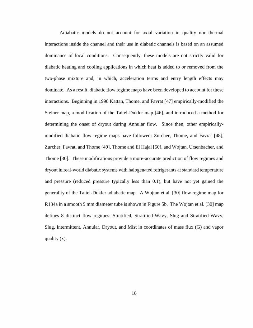
18
Adiabatic models do not account for axial variation in quality nor thermal
interactions inside the channel and their use in diabatic channels is based on an assumed
dominance of local conditions. Consequently, these models are not strictly valid for
diabatic heating and cooling applications in which heat is added to or removed from the
two-phase mixture and, in which, acceleration terms and entry length effects may
dominate. As a result, diabatic flow regime maps have been developed to account for these
interactions. Beginning in 1998 Kattan, Thome, and Favrat [47] empirically-modified the
Steiner map, a modification of the Taitel-Dukler map [46], and introduced a method for
determining the onset of dryout during Annular flow. Since then, other empirically-
modified diabatic flow regime maps have followed: Zurcher, Thome, and Favrat [48],
Zurcher, Favrat, and Thome [49], Thome and El Hajal [50], and Wojtan, Ursenbacher, and
Thome [30]. These modifications provide a more-accurate prediction of flow regimes and
dryout in real-world diabatic systems with halogenated refrigerants at standard temperature
and pressure (reduced pressure typically less than 0.1), but have not yet gained the
generality of the Taitel-Dukler adiabatic map. A Wojtan et al. [30] flow regime map for
R134a in a smooth 9 mm diameter tube is shown in Figure 5b. The Wojtan et al. [30] map
defines 8 distinct flow regimes: Stratified, Stratified-Wavy, Slug and Stratified-Wavy,
Slug, Intermittent, Annular, Dryout, and Mist in coordinates of mass flux (G) and vapor
quality (x).

19
Figure 5: a) Taitel-Dukler [46] adiabatic flow regime map and b) Wojtan et al. [30] diabatic flow
regime map for evaporation of R134a at -15ºC in a 9mm smooth tube with a heat flux of 4 kW/m²
Recently, there has been a renewed interest in the use of CO2, as an environmentally
friendly alternative refrigerant, and halogenated refrigerants at high reduced pressure for
clothes dryers [51], solar assisted heat pumps [52], and electronic cooling applications [53].
Thome and Ribatski [39] published a comprehensive review of smooth tube flow boiling
of CO2 and found that the high reduced pressure and associated high vapor density, low
surface tension, high vapor viscosity, and low liquid viscosity resulted in significant flow
regime and heat transfer variations compared to traditional refrigerants. Consequently, the
available diabatic flow regime maps described above did not adequately predict flow
regimes for CO2. In response, Mastrullo et al. [54] collected heat transfer and flow regime
measurements for CO2 and R410A at reduced pressures from 0.19 to 0.64 and developed
new ‘easy to use’ semi-empirical models to improve predictive accuracy at high reduced
pressure.
It’s interesting to note that the Taitel-Dukler [46] and Wojtan et al. [30] flow regime
maps in Figure 5 share distinct similarities, such as the general locations of the dominant
0
100
200
300
400
500
0 0.1 0.2 0.3 0.4 0.5 0.6 0.7 0.8 0.9 1
G (
kg/m
²s)
x
Intermittent
Annular
Stratified0
100
200
300
400
500
0 0.1 0.2 0.3 0.4 0.5 0.6 0.7 0.8 0.9 1
G (
kg/m
²s)
x
Intermittent
Annular
Slug
Slug and
Stratified
-Wavy
Mist
Dryout
Stratified
Stratified-Wavy
(b)
(b) (a)
20
flow regimes, but the transitions from one flow regime to the next occur at significantly
different mass fluxes and vapor qualities. In addition, creating the Taitel-Dukler map [46]
requires complex calculations and an iterative process to determine the extent of each
regime, while rather simple calculations are required to implement the Wojtan et al. [30]
and Mastrullo et al. [54] maps, to describe the loci of flow regime transitions. Therefore,
the Wojtan et al. [30] and Mastrullo et al. [54] maps will be used herein as diagnostic tools
and to provide a baseline for the evaluation of flow regime transition in internally-grooved
tubes with refrigerants at standard and reduced pressure, respectively.
Regarding applicability to a range of working fluids and channel sizes, the database
used to create the most-recent Wojtan et al. [30] flow regime map covers data from three
common refrigerants, namely R134a, R22, and R410A, but only a limited range of internal
diameters, from 12 to 14 mm. The Mastrullo et al. [54] flow regime map was validated
using one 6 mm diameter smooth tube, reduced pressure from 0.57 to 0.64 for CO2 and
0.19 to 0.52 for R410A, mass fluxes from 150 to 500 kg/m²s, and heat fluxes between 5
and 20 kW/m². Since these models originated with the physics-based transition criteria of
Taitel-Dukler [46], it is expected that they will apply to a wider range of tube diameters
and fluids than that presented in the validating data set.
It is to be noted that unlike the eight unique flow regimes defined by the Wojtan et
al. [30] map, most two-phase researchers [55] have limited their classification to the
previously described primary flow regimes. In the interest of uniformity and consistency,
and to avoid confusion that may derive from the diversity of names used by authors for
some of the observed sub-regimes, the present effort will follow the classification proposed
by Rahim et al. [55], combining Slug, Plug, and Intermittent data points into Intermittent

21
flow, combining Slugging-Annular flow, Wavy-Annular flow, and Semi-Annular data into
Annular flow, and defining Stratified-Wavy flow as a sub-regime of Stratified flow,
leading to the presence of just 4 primary regimes: Stratified, Bubbly, Intermittent, and
Annular.
2.3 Smooth Tube Regime-Based Heat Transfer Models
As shown schematically in Figure 4, the heat transfer coefficient during two-phase
flow is generally dependent on the predominant flow regime and, in diabatic flow, varies
axially as the quality changes from the inlet to the outlet of the channel. Therefore, accurate
prediction of two-phase heat transfer coefficients requires prediction and knowledge of the
prevailing flow regime and its axial progression. Despite this fact, the most widely used
heat transfer coefficient correlations are empirical, failing to incorporate flow structure in
the prediction method, or based on a physical representation of a specific flow regime but
used indiscriminately across all the prevailing regimes, as for example with the smooth
tube correlations of Chen [56], Shah [57], Kandlikar and Balasubramanian [58], and
Gungor and Winterton [59] [60]. Studies such as the one by Bar-Cohen and Rahim [35]
suggest that substantially improved predictive agreement can be achieved when the
selection of a correlation includes consideration of its phenomenological underpinnings.
To more accurately capture the regime-dependent performance during diabatic
flow in tubes, Kattan et al. [61] [62] developed the first comprehensive flow pattern based
heat transfer model. Based on the predicted flow regime, the Annular film thickness,
turbulence, and dry perimeter during Stratified flows were determined and used to calculate
the local heat transfer coefficient. The Kattan, Thome, and Favrat flow regime and heat
transfer models [61] [62] have since been modified by other researchers. Each successive

22
flow regime map, as described above, had an accompanying regime-based heat transfer
coefficient correlation. The most recent version, as developed by Wojtan et al. [31],
includes the onset of nucleate boiling as defined by Zurcher at al. [49], a Dryout and Mist
flow regime at high vapor quality, and a more detailed description of the Stratified-Wavy
sub-regime of Stratified flow.
As an example of the power of this regime-based approach, Figure 6 shows a
comparison of two-phase data from Filho and Jabardo [38] with the predicted heat transfer
coefficient and the flow regime map from Wojtan et al. [30] for flow boiling in an 8.92
mm ID tube with R134a at a saturation temperature of 5ºC and mass fluxes of 100 and 300
kg/m²s.
Figure 6: Comparison of experimental heat transfer data (adapted from Filho and Jabardo [38])
(hollow data points) for R134a at 5ºC in an 8.92 mm smooth tube with a heat flux of 5 kW/m² to a)
the Wojtan et al. heat transfer model [31] and b) Wojtan et al. flow regime map [30]
At a mass flux of 100 kg/m²s, the locus of which is shown in Figure 6b, the model
correctly predicts a low heat transfer coefficient characteristic of Stratified flow and a large
dry perimeter. When the flow regime transitions from Intermittent to Annular flow at a
0
2000
4000
6000
8000
10000
0 0.1 0.2 0.3 0.4 0.5 0.6 0.7 0.8 0.9 1
Hea
t tr
ansf
er c
oef
fici
ent
(W/m
²K)
x
0
100
200
300
400
500
0 0.1 0.2 0.3 0.4 0.5 0.6 0.7 0.8 0.9 1
G (
kg/m
²s)
x
Intermittent
Annular
Mist
Dryout
Stratified
Slug
Slug and
Stratified-
Wavy
100 kg/ms experimental 300 kg/ms experimental 100 kg/ms experimental 300 kg/ms experimental100 kg/m²s exp. 300 kg/m²s exp. 100 kg/m²s calc. 300 kg/m²s calc.
(b) (a)

23
mass flux of 300 kg/m²s, as may be seen from the locus shown in Figure 6b, the model
predicts an increase in heat transfer coefficient due to enhanced convective cooling and a
thinning Annular film. Additionally, the heat transfer coefficient correlation correctly
predicts the smooth transition between the respective flow regimes and the sharp reduction
at high vapor qualities due to dryout.

24
Chapter 3: Fundamental Studies of Flow Patterns and Heat
Transfer in Internally-Grooved Tubes
Two-phase flow boiling in internally-grooved tubes has been a subject of interest
since they were invented in 1977, with notable reviews by Thome of internally-grooved
tube studies prior to 1990 [11], a quality general review by Bergles and Manglik [63], and
an update on boiling heat transfer inside enhanced tubes published by Thome in 2004 [17].
Since early 2000, there have been a large number of studies in the literature exploring
evaporative heat transfer in internally-grooved tubes but few, if any, researchers have made
an effort to compile this data and analyze the relationship between flow regime and
evaporative heat transfer rates.
Based on this apparent void in the literature and the demonstrated success of
regime-based analyses and correlations in providing improved predictive accuracy for heat
transfer coefficients in smooth tubes, as described in Chapter 2, this chapter aims to explore
the relationship between two-phase flow regimes and heat transfer rates in internally-
grooved tubes. First, fundamental studies of thermofluid performance in internally-
grooved tubes are reviewed and compared to the Wojtan et al. [30] and Mastrullo et al. [54]
flow regime maps. Then, the current state of two-phase flow regime maps and heat transfer
coefficient correlations for internally-grooved tubes is described. Finally, results and
general comments are summarized and research directions for the current effort are
developed. The majority of studies, reviewed herein, deal with halogenated fluids in
conventional-sized tubes at standard temperature and pressure. However, studies of small
diameter tubes, as well as alternative refrigerants and operation at reduced pressure, are

25
also considered. The majority of this chapter was published as a paper in the Journal of
Enhanced Heat Transfer by Sharar and Bar-Cohen [64].
3.1 Flow Regime Quantification
Although the common flow regime definitions are typically based on visual and
verbal descriptions, the complex nature of two-phase flow limits the accuracy and utility
of such subjective determinations of flow models [65]. Regrettably, the majority of the
studies to be discussed in the following chapter relied solely on subjective flow regime
determination methods. These studies provide an adequate starting point for developing a
physical relationship between flow regime and heat transfer in internally-grooved tubes,
however, more subjective techniques will be needed to firmly establish the nature and
repeatability of the dependence of thermal and momentum transport on the prevailing flow
regime in such tubes. The reader is referred to Chapter 6 for a more detailed description
of subjective determination techniques in the literature and the Total Internal Reflection
technique used in the current study.
3.2 Studies on Conventional Internally-Grooved Tubes
The majority of the experiments focusing on flow regime and heat transfer in
internally-grooved tubes have been conducted in conventional tubes ranging in size from
5 to 15 mm. Such tubes are more widely available and have been extensively tested,
whereas tubes smaller than 5 mm have only recently gained attention. Table 4 is a
summary of relevant studies of flow pattern and heat transfer in ‘meso’-sized internally-
grooved tubes, focusing on studies that demonstrate heat transfer improvement through
early flow regime transition. Most of the studies examined used refrigerant - refrigerant
vapor (of a single fluid) under diabatic conditions and standard temperature and pressure.

26
Some studies explored halogenated fluids and CO2 at high reduced pressure while others
explored refrigerant/oil mixtures. Several studies used adiabatic water - air as the working
fluids.
Table 4: Summary of relevant studies on flow patterns and heat transfer in macroscale internally-
grooved tubes
Authors/References Fluid and test section description Main research content
Yu, Lin, and Tseng [66]
R134a evaporation, 1.5 m horizontal
smooth and internally-grooved tube,
10.7 mm ID
Flow regime was mapped for both
tubes, heat transfer coefficient was
measured, new heat transfer coefficient
correlation was developed
Oh and Bergles [67]
R134a evaporation, one smooth and 3
internally-grooved tubes with helix
angles of 6º, 18º, and 44º, horizontal
9.52 mm ID tubes
Used a boroscope visualization
technique to relate fluid redistribution
to helix angle
Shedd and Newell [27]
Adiabatic water-air, 0.8 m horizontal
smooth and internally-grooved PVC
tubing, 15.1 mm ID
Flow regime, pressure drop, and
circumferential Annular film thickness
were measured
Shedd, Newell, and Lee [68]
Adiabatic water-air, 0.8 m horizontal
smooth and internally-grooved PVC
tubing, 15.1 mm ID
Flow regime, pressure drop, and
circumferential Annular film thickness
were measured, influence of number
and angle of microgrooves was
reported
Shen and Groll [69]
A critical review of lubricant
influence on pool and flow boiling in
smooth and enhanced tubes
Comprehensive summary of recent
work and technical recommendations
Kim Shin [26]
R22 and R410A evaporation, 0.92 m
horizontal smooth, 5 internally-
grooved, and 1 herringbone tube,
8.14-8.7 mm ID
Heat transfer coefficient was measured
for all tubes, heat transfer data
compared to heat transfer coefficient
correlations available in the literature
Schael and Kind [70]
Reduced pressure CO2 evaporation,
0.2 m horizontal internally-grooved
tube, 8.62 mm ID
Flow regime was mapped, heat transfer
coefficient was measured and
compared to previous smooth tube data
Filho and Jabardo [38]
R134a evaporation, 1.5 m horizontal
smooth, herringbone, and internally-
grooved tube, 8.76-8.92 mm ID
Flow visualization for smooth and
internally-grooved tubes, heat transfer
coefficient and pressure drop were
measured
Cho and Kim [71] Reduced pressure CO2 evaporation,
0.2 m horizontal internally-grooved
tube, 8.62 mm ID
Heat transfer coefficient and pressure
drop was measured and compared to
heat transfer coefficient and pressure
drop correlations available in the
literature
Targanski and Cieslinski [72]
R407C and R407C/oil mixture
evaporation in two smooth tubes, one
corrugated tube, and one internally-
grooved tube, 2 m long, 8-8.92 mm
ID
Heat transfer coefficient and pressure
drop was measured for all tubes

27
Hu, Ding, and Wang [73]
R410A and R410A-oil mixture
evaporation in a 7 mm OD internally-
grooved tube
Heat transfer coefficient was measured
for nominal oil concentrations from 0-
5%, new heat transfer coefficient
correlation was developed
Spindler and Müller-Steinhagen
[74]
R134a and R404A evaporation, two
0.5 m horizontal internally-grooved
tubes, 8.95 mm ID
Flow regime was mapped for both
fluids, heat transfer coefficient was
measured and compared to correlations
in the literature, modified constants on
existing heat transfer coefficient
correlation
Filho and Barbieri [75]
R134a evaporation, 1.5 m horizontal
smooth and two internally-grooved
tubes, 8.92 mm ID
Flow visualization for both tubes, heat
transfer coefficient and pressure drop
were measured
Padovan et al. [76]
Reduced pressure (0.19-0.49) R134a
and R410A evaporation, 0.3 m
horizontal internally-grooved tube,
8.15 mm ID
heat transfer coefficient and dryout
vapor quality were measured and
compared to correlations available in
the literature, new dryout inception
model was developed
Hatamipour and Akhavan-
Behabadi [77]
R134a evaporation, 1.1 m horizontal
smooth and internally-grooved tube,
8.92 mm ID
Flow regime was mapped for both
tubes, heat transfer coefficient was
measured
Zhao and Bansal [78] Reduced pressure CO2 evaporation, 1
m horizontal internally-grooved tube,
7.3 mm ID
Heat transfer coefficient was measured
and compared to heat transfer
coefficient correlations available in the
literature
Colombo et al. [79]
R134a evaporation, 1.3 m horizontal
smooth and two internally-grooved
tubes, 8.62-8.92 mm ID
Flow regime was mapped on existing
maps, pressure drop and heat transfer
coefficient were measured and
compared to correlations available in
the literature
Sharar and Bar-Cohen [80] HFE-7100 evaporation, 0.2 m
horizontal smooth and internally-
grooved tubes, 8.84 mm ID
Flow regime was mapped and heat
transfer coefficient was measured for
both tubes. New heat transfer
coefficient was introduced based on
previous flow regime map [29]. Model
matched well with results and data from
3 independent researchers.
3.2.1 Flow Regime Transition Mechanisms
The smooth tube regime transition from Stratified to Annular flow is modeled in
the Taitel-Dukler flow regime map [46] by the waves produced due to the Kelvin-
Helmholtz instability or the impingement of liquid drops on the upper surfaces, while the
Intermittent to Annular transition is modeled by the rupture of the liquid plug by the vapor
flow. Annular flow in internally-grooved tubes appears to exist at lower mass flux and

28
vapor quality than in smooth tubes [29], suggesting that the physics of flow regime
transition in internally-grooved tubes is more complex. In addition to the inertial and
surface tension effects mentioned above, it is believed that fluid flow redirection from axial
to helical flow in the grooves (momentum change), as well as capillary force in the groove
structures, and centrifugal force due to flow circulation, play a role in early transition to
Annular flow in these tubes.
Shedd and Newell [27] [81] [82] [68] used a non-intrusive optical film thickness
measurement technique to observe the liquid distribution in horizontal adiabatic water-air
flow through 15.1 mm ID smooth and internally-grooved tubes with helix angles of 9° and
18°. These studies demonstrated the impact of grooves on liquid redistribution and early
transition to Annular flow in internally-grooved tubes. Liquid film thickness profiles for
Stratified/Annular flow through 15.1 mm smooth and internally-grooved tubes at mass
fluxes of 44 and 120 kg/m²s are shown schematically in Figure 7. Additionally, these data
points are plotted on the Wojtan et al. [30] flow regime map. The smooth tube films are
represented by dotted lines and the grooved tube film thicknesses are shown with solid
lines.
At low mass flux, 44 kg/m²s, the smooth tube profiles were symmetric from left to
right with thicker liquid films on the bottom and dry patches at the top surface; this can be
identified as Stratified flow and corresponds to a Stratified-Wavy regime on the Wojtan et
al. map [30]. The grooved tube profiles appeared to be rotated counterclockwise (the same
direction as the groove), achieving wetting of nearly 94% of the periphery vs only 62% for
the smooth tube, and displaying behavior that can be identified as Annular flow. Shedd
and Newell [27] also reported that the liquid film profiles for the smooth and internally-

29
grooved tubes tended to converge at higher mass flux, as seen in the film profiles for 120
kg/m²s, corresponding to Annular flow on the Wojtan et al. [30] map in Figure 7. The
preferential redistribution of liquid in the direction of the helical grooves, achieving greater
wetting at low mass fluxes, supports the existence of a secondary Stratified-to-Annular
flow regime transition mechanism in internally-grooved tubes and could be expected to
lead to higher heat transfer coefficients. Moreover, the similarity in film profiles at the
higher mass fluxes would appear to be consistent with the decrease in enhancement at
higher mass flux, as reported in the literature and outlined in Table 3.
Based on heat transfer experiments with liquid capillary rise on grooved flat plates,
Kimura and Ito [83] and Ito and Kimura [84] hypothesized that capillary force in the
grooves is a dominant factor for enhanced heat transfer in internally-grooved tubes.
Essentially, the capillary force works to redistribute fluid from the bottom or sides of the
tube to the top. This mode of enhancement in internally-grooved tubes has also been
suggested by Yoshida et al. [85] [86] and Cui et al. [87] .
Figure 7: Film thickness profiles for smooth (dashed lines) and 18° internally-grooved (solid red
lines) tubes with 15.1 mm ID and mass fluxes of a) G=44 kg/m²s and x=0.6 and b) G=120 kg/m²s and
x=0.76 [27], plotted on the simplified Wojtan et al. [30] flow regime map
0
100
200
300
400
500
0 0.1 0.2 0.3 0.4 0.5 0.6 0.7 0.8 0.9 1
G (
kg/m
²s)
x
Stratified
Annular
Intermittent
Dryout
Mist
Stratified-Wavy
Slug
Slug and
Stratified-
Wavy
(c)
(b) (a)

30
3.2.2 Halogenated Fluids at Standard Pressure and Temperature
Yu, Lin, and Tseng [66] performed a flow visualization and heat transfer study with
R134a at 6ºC in a 10.7 mm ID smooth and an 11.1 mm ID internally-grooved tube with an
18° helix angle. Mass fluxes from 163 to 408 kg/m²s, heat flux between 2.2 and 56 kW/m²,
and a fixed heated length of 1.5 m were tested. Figure 8 shows the results of the flow
visualization, plotted in the coordinates of mass flux and vapor quality and superimposed
on the Wojtan et al. [30] flow regime map; Figure 8a is the smooth tube experimental
results and Figure 8b is the internally-grooved tube results. The transitions of flow pattern
visually observed were Stratified, Intermittent, and Annular in the direction of increasing
mass flux and vapor quality.
It was reported in the study, and also apparent from Figure 8, that the transitions in
the internally-grooved tube occurred at lower mass flux and vapor quality compared with
the smooth tube. Thus, at a mass flux of 163 kg/m²s and a quality greater than 0.3, Annular
flow was encountered in the internally-grooved tube while the smooth tube was operating
in the Stratified regime. Additionally, at a mass flux of 245 kg/m²s and a quality greater
than 0.15, Annular flow was encountered in the internally-grooved tube while the smooth
tube was operating in the Intermittent regime. The Wojtan et al. [30] flow regime map was
shown to satisfactorily predict flow regime in the smooth tube, but due to the observed
early flow regime transition in the internally-grooved tube at lower mass flux and vapor
quality, the Wojtan et al. [30] map did a poor job predicting flow regimes in the internally-
grooved tube [29].

31
Figure 8: Experimental flow visualization results from Yu et al. [66] for R134a at 6ºC with a heat
flux of 20 kW/m² plotted on a simplified Wojtan et al. [30] map for a) 10.7 mm ID smooth tube and
b) 11.1 mm ID internally-grooved tube
The aforementioned early flow regime transitions at low mass flux improved heat
transfer in the internally-grooved tube relative to the smooth tube. Figure 9a shows the
average heat transfer coefficient vs. vapor quality for a mass flux of 163 kg/m²s and Figure
9b shows the internally-grooved enhancement factor. The enhancement factor is defined
as the ratio of the internally-grooved tube heat transfer coefficient to the smooth tube heat
transfer coefficient. The additional area provided by the internally-grooved tube of Yu,
Lin, and Tseng [66] was accounted for in Figure 9, resulting in a smooth tube equivalent
heat transfer coefficient.
As can be seen in Figure 9a, the increase in the smooth tube heat transfer coefficient
was minimal due to the dominance of Stratified flow. Alternatively, when the flow pattern
was changing, the rise in the heat transfer coefficient was dramatic. At a mass flux of 163
kg/m²s and quality of 0.3 there was a sharp increase in the heat transfer coefficient, from
0
100
200
300
400
500
0 0.1 0.2 0.3 0.4 0.5 0.6 0.7 0.8 0.9 1
G (
kg/m
²s)
x
Intermittent
Annular
Mist
Dryout
Stratified
Stratified-Wavy
Slug and
Stratified-
Wavy
Slug
0
100
200
300
400
500
0 0.1 0.2 0.3 0.4 0.5 0.6 0.7 0.8 0.9 1
G (
kg/m
²s)
x
Intermittent
Annular
Mist
Dryout
Stratified
Stratified-Wavy
Slug and
Stratified-
Wavy
Slug
1 1 1Stratified
(b)
Annular Intermittent
(b) (a)

32
approximately 4 to 5.5 kW/m²K (40% improvement), accompanying the flow regime
transition from Intermittent to Annular flow in the internally-grooved tube. Consequently,
the maximum heat transfer enhancement of 2.25, as shown in Figure 9b, occurred at a flow
rate of 163 kg/m²s and qualities 0.3<x<0.7 where Stratified flow dominated in the smooth
tube and flow transition to Annular was achieved in the internally-grooved tube.
Figure 9: a) Heat transfer coefficient vs vapor quality and b) accompanying enhancement factor
from several researchers with low mass flux (100 – 163 kg/m²s)
As may be seen in Figure 8a, at a mass fluxes of 326 kg/m²s or above, the observed
flow regimes for the smooth and internally-grooved tubes tended to converge to Annular
flow. Figure 10a and Figure 10b show the average heat transfer coefficient vs. vapor
quality for the smooth tube and internally-grooved tube and the enhancement factor at the
higher mass flux of 326 kg/m²s. As can be seen in Figure 10a, a significant increase in
heat transfer coefficient is observed in the smooth tube at a mass flux of 326 kg/m²s and a
vapor quality of 0.2, coinciding with transition to Annular flow and yielding a smooth tube
0
1000
2000
3000
4000
5000
6000
7000
8000
9000
0 0.1 0.2 0.3 0.4 0.5 0.6 0.7 0.8 0.9 1
Hea
t tr
ansf
er c
oef
fici
ent
(W/m
²K)
x
0
1
2
3
4
5
6
7
0 0.1 0.2 0.3 0.4 0.5 0.6 0.7 0.8 0.9 1
Enhan
cem
ent
fact
or
(hIG
/hsm
ooth
)
x
Filho Barbieri smooth Filho Barbieri smooth Filho Barbieri smooth
Filho Barbieri smooth Filho Barbieri smooth Filho Jabardo smooth
Filho Barbieri smooth Filho Barbieri smooth Filho Barbieri smooth
(b)
Yu et al.
smooth
Filho-Barbieri IG 1
Filho-Jabardo IG
Yu et al. IG
Filho-Barbieri IG 2
Colombo et al. IG 1
Filho-Barbieri smooth
Filho-Jabardo smooth
Colombo et al. IG 2
(b) (a)

33
heat transfer coefficient profile that more closely resembles that of the internally-grooved
tube. Calculation of the internally-grooved tube enhancement factor reveals that the heat
transfer improvement approaches 1.3 at high mass flux and high vapor quality. The
marginal improvement beyond area enhancement at higher mass fluxes may be a result of
extra turbulence, mixing, or nucleate boiling due to the grooved structures. These trends
are consistent with trends discussed in Table 3, and as described, are directly related to the
observed flow regime. The experimental data were compared with existing smooth tube
correlations from Kattan et al. [62], Chen [56], Shah [57], Gungor and Winterton [60], Liu
and Winterton [88] and a newly-proposed heat transfer coefficient correlation by Yu, Lin,
and Tseng [66]. Their experimental data was found to correlate well with the most recent
heat transfer coefficient correlation.
Figure 10: a) Heat transfer coefficient vs vapor quality and b) accompanying enhancement factor
from several researchers with high mass flux (300 - 326 kg/m²s)
0
1000
2000
3000
4000
5000
6000
7000
8000
9000
0 0.1 0.2 0.3 0.4 0.5 0.6 0.7 0.8 0.9 1
Hea
t tr
ansf
er c
oef
fici
ent
(W/m
²K)
x
0
1
2
3
4
5
6
7
0 0.1 0.2 0.3 0.4 0.5 0.6 0.7 0.8 0.9 1
Enhan
cem
ent
fact
or
(hIG
/hsm
ooth
)
x
Filho Barbieri smooth Filho Barbieri smooth Filho Barbieri smooth
Filho Barbieri smooth Filho Barbieri smooth Filho Jabardo smooth
Filho Barbieri smooth Filho Barbieri smooth Filho Barbieri smooth
(b) (a)
Yu et al. smooth
ssmoothsmooth
Filho-Barbieri IG 1
Filho-Jabardo IG
Yu et al. IG
Filho-Barbieri IG 2
Colombo et al. IG 1
Filho-Barbieri smooth
Filho-Jabardo smooth
Colombo et al. IG 2
34
Bandarra Filho and co-workers [75] [38] reported experimental investigations of
flow boiling of R134a in a smooth tube and two internally-grooved tubes with inside
diameters of 8.76 to 8.92 mm, helix angles of 18°, fin heights of 0.2 mm, and between 60
and 80 grooves. Tests were performed in 1.5 m long tubes with a saturation temperature
of 5°C, a heat flux of 5 kW/m², vapor qualities up to 90%, and mass fluxes from 100 to
500 kg/m²s. The area enhancement of the internally-grooved tube was 1.91 times the
smooth tube in the Filho and Jabardo [38] study but was not reported in the Filho and
Barbieri [75] study. Filho and Barbieri [75] provided representative flow regime
photographs for several operating conditions and described the flow regime trends but did
not plot their flow visualization data.
Figure 11 shows the Filho and Barbieri [75] flow regime data plotted on a Wojtan
et al. [30] flow regime map. For the smooth tubes they visually observed that Annular flow
was the dominant regime at high vapor quality and mass flux greater than 150 kg/m²s. For
mass fluxes higher than 150 kg/m²s and low vapor quality, Intermittent flow was the
dominant regime. At mass velocities lower than 150 kg/m²s, Stratified flow was observed
for the entire range of vapor qualities tested. These trends are captured well by the Wojtan
et al. [30] flow regime map.
The trends were different in the internally-grooved tubes. Stratified flow was never
observed in the internally-grooved tubes, even at mass fluxes as low as 100 kg/m²s.
Instead, earlier transition to Intermittent and Annular flow was reported at lower mass flux
and vapor quality than observed in the smooth tube. One specific example on Figure 11 is
at a mass flux of 300 kg/m²s and a vapor quality of 0.1 where the smooth tube was operating
in Stratified flow while the internally-grooved tube was operating in Annular flow. It’s
35
also interesting to point out that at a mass flux of 500 kg/m²s and a vapor quality around
0.65, the smooth tube was operating in Annular flow and the internally-grooved tube
prematurely transitioned to Mist flow. Similar flow regime trends were reported by Filho
and Jabardo [38] for similar test conditions.
Figure 11: Experimental flow visualization results of Filho and Barbieri [75] for R134a at 5ºC in an
8.92 mm smooth and internally-grooved tube with a heat flux of 5 kW/m² plotted on a simplified
Wojtan et al. [30] flow regime map
Figure 9a shows the average heat transfer coefficient vs. vapor quality for the
smooth tube and three internally-grooved tubes at a mass flux of 100 kg/m²s for Filho and
Barbieri [75] and Filho and Jabardo [38]. It’s important to note that - in these studies - the
increased internally-grooved tube surface area was not accounted for when calculating the
heat transfer coefficient, so it’s expected that the heat transfer coefficient should be close
to 1.3 to 1.91 times larger than the smooth tube values for all test conditions. At a mass
flux of 100 kg/m²s the heat transfer coefficient in the smooth tube is low and appears to
slightly deteriorate over the whole range of vapor qualities; this is indicative of the
0
100
200
300
400
500
0 0.1 0.2 0.3 0.4 0.5 0.6 0.7 0.8 0.9 1
G (
kg/m
²s)
x
IG - Annular Smooth - Stratified Smooth - Annular IG - Mist
Smooth - Intermittent
Smooth - Annular
Smooth - Stratified
Smooth - Intermittent
Smooth - Intermittent IG - AnnularIntermittent
Stratified
Mist
Annular
Dryout
Slug
Slug and
Stratified-
Wavy Stratified-Wavy

36
observed Stratified flow regime at mass fluxes below 150 kg/m²s. Under the same
conditions, the heat transfer coefficient increases in all of the internally-grooved tubes. As
described above, this is a result of the dominance of Intermittent and Annular flow in the
internally-grooved tube. As shown in Figure 9b, the effect is heat transfer enhancement
close to 6 times that of the plain tube. However, at a higher mass flux of 300 kg/m²s, where
Intermittent and Annular flow were the dominant regimes in both the smooth and
internally-grooved tubes, the heat transfer trends begin to converge to the internal area
enhancement. This effect is clearly shown in Figure 10a and b.
Additionally, at a mass flux of 500 kg/m²s and vapor quality above 0.5, Filho and
Barbieri [75] and Filho and Jabardo [38] reported worse performance in the internally-
grooved tubes compared to the smooth tube as a result of the premature transition to Mist
flow. The results were not compared to existing internally-grooved tube heat transfer
coefficient correlations. It’s interesting to note that Filho and Jabardo [38] and Filho and
Barbieri [75] reported similar trends with respect to flow regime and thermal performance,
however, subtle differences in performance between the two studies can be seen in Figure
9 and Figure 10, presumably as a result of varying geometric parameters.
Colombo et al. [79] performed a flow visualization and evaporative/condensing
heat transfer study with R134a at a saturation temperature of 5°C in a horizontal 8.92 mm
ID smooth tube and two internally-grooved tubes with inside diameters of 8.62 and 8.92
mm. Both internally-grooved tubes had helix angles of 18° and apex angles of 40º, but had
alternating fin heights ranging from 0.16 to 0.23 mm and the number of grooves ranging
from 54 to 82. The resulting internally-grooved tube area enhancement ranged from 1.55
to 1.82. Mass fluxes from 100 to 340 kg/m²s, heat flux between 2.2 and 56 kW/m², vapor

37
qualities from 0.1 to 0.9, and a fixed heated length of 1.3 m were tested. Figure 12 shows
the results of the flow visualization, plotted in the coordinates of mass flux and vapor
quality and superimposed on the Wojtan et al. [30] flow regime map; Figure 12a is the
smooth tube experimental results and Figure 12b is the results for one of the internally-
grooved tubes. The transitions of flow pattern visually observed were Stratified,
Intermittent, and Annular in the direction of increasing mass flux and vapor quality.
Figure 12: Flow visualization results from Colombo et al. [79] for 8.92 mm ID a) smooth and b)
internally-grooved tubes with R134a at 5ºC and a heat flux of 4.2 kW/m² plotted on the Wojtan et al.
[30] flow regime map
Figure 12 makes it very clear that there are distinct differences in flow regimes
between the smooth and internally-grooved tubes, with the latter shifting the onset of
Annular flow to lower mass flux and vapor quality. One example is at a mass flux of 100
kg/m²s and a quality greater than 0.4 where Annular flow was encountered in the internally-
grooved tube, while the smooth tube was operating in the Stratified regime. Additionally,
at vapor qualities close to 0.3 and mass fluxes greater than 180 kg/m²s, the smooth tube
was operating in Intermittent flow and the internally-grooved tube was operating in
0
100
200
300
400
500
0 0.1 0.2 0.3 0.4 0.5 0.6 0.7 0.8 0.9 1
G (
kg/m
²s)
x
Intermittent
Annular
Mist
Dryout
Stratified
Stratified-Wavy
Slug and
Stratified-
Wavy
Slug
0
100
200
300
400
500
0 0.1 0.2 0.3 0.4 0.5 0.6 0.7 0.8 0.9 1
G (
kg/m
²s)
x
Intermittent
Annular
Mist
Dryout
Stratified
Slug
Slug and
Stratified-
Wavy Stratified-Wavy
1 1 1Stratified Intermittent Annular
(b) (a)

38
Annular flow. Annular flow was observed in both the smooth and internally-grooved tubes
at high mass flux and vapor quality. The Wojtan et al. [30] flow regime map accurately
predicted flow regime and flow regime transitions in the smooth tube, but due to the
observed early flow regime transition in the internally-grooved tube at lower mass flux and
vapor quality, the Wojtan et al. [30] map was unable to properly predict flow regimes in
the internally-grooved tube.
Due to limitations in the data of Colombo et al. [79], it could not be included in the
overall plot of the heat transfer coefficient vs vapor quality, Figure 9a and Figure 10a.
However, they reported enhancement factors at an average vapor quality of 0.45 for mass
fluxes ranging from 90 to 320 kg/m²s and these values were added to the enhancement
factor plots, Figure 9b and Figure 10b. As shown in Figure 9b, the heat transfer
enhancement at a mass flux of 90 kg/m²s and mean vapor quality of 0.45 was 2.4 to 2.7
times higher than the smooth tube. This corresponds to Annular flow in the internally-
grooved tube and Stratified flow in the smooth tube. As shown in Figure 10b, at a higher
mass flux of 320 kg/m²s and the same vapor quality where Annular flow is the dominant
regime in both the smooth and internally-grooved tubes, the enhancement ratio reduces to
1.35 for both internally-grooved tubes. It is to be noted that Colombo et al. [79] did not
account for the increased internally-grooved tube surface area when calculating the heat
transfer coefficient. So, it’s to be expected that the heat transfer enhancement should be at
least 1.55 to 1.82 times larger than the smooth tube values for all test conditions. The
researchers did not comment on this discrepancy. Though not explicitly described here,
it’s important to note that the Colombo et al. [79] results showed performance differences

39
between the two internally-grooved tubes, which reinforces that the specific geometric
parameters may affect thermal performance.
The internally-grooved tube experimental data was compared with existing
internally-grooved correlations from Murata et al. [89], Yun et al. [90], and Thome et al.
[91]. The measured heat transfer coefficients were not well correlated by any of the
existing correlations, with average percent errors ranging from -39% to +156%.
Spindler and Müller-Steinhagen [74] performed an experimental investigation of
heat transfer and flow regime during evaporative cooling in an 8.92 mm ID internally-
grooved tube with a 15° helix angle using two different refrigerants, R134a and R404A.
Experiments were conducted in a 1 m long heated test section with mass fluxes ranging
from 25 to 150 kg/m², heat flux from 1 to 15 kW/m², inlet vapor qualities ranging from 0.1
to 0.7, and a saturation temperature of -20ºC. Stratified, Intermittent, and Annular flow
were observed. Annular flow was the dominant regime for mass fluxes at or above 65
kg/m²s. Shown in Figure 13 is the experimental visual flow regime data of Spindler and
Müller-Steinhagen [74] for R134a and R404A plotted on the Wojtan et al. [30] flow regime
map.
The Wojtan et al. [30] map over-predicts the mass flux at which transition from
Stratified to Annular flow occurs for both fluids. They hypothesized that the spiral grooves
worked to redistribute the liquid, resulting in early transition to Annular flow.
Unfortunately they did not perform flow regime and heat transfer experiments for a
comparable smooth tube as a benchmark for comparison. The experimental heat transfer
coefficients were compared to the correlations from Koyama et al. [92] and Kandlikar [93]
and average deviations of ±15% and ±30%, respectively, were observed.

40
Figure 13: Experimental flow visualization results from Spindler and Müller-Steinhagen [74] for a)
R134a and b) R404A at -20ºC with a heat flux of 7.5 kW/m² in one 8.92 mm ID internally-grooved
tube plotted on a corresponding Wojtan et al. [30] flow regime map
3.2.3 Refrigerant/Oil Mixtures
In operating refrigeration systems, it is not uncommon to encounter boiling of
refrigerant/oil mixtures. The amount of oil in the mixture, which is dependent on system
wear and worker expertise, will increase pressure drop and may help or hinder cooling
performance. Therefore, it is essential to test flow boiling of refrigerant/oil mixtures for a
wide range of test conditions and a wide range of refrigerants and oils. While not the main
intent of the current research effort, several representative reviews and studies [72] [73]
[69] on the performance of refrigerant/oil mixtures in internally-grooved tubes have been
included in Table 4 for the sake of completeness.
3.2.4 Halogenated Fluids and CO2 at Elevated Reduced Pressure
Most macro-channel internally-grooved tube flow boiling studies in the open
literature are concerned with halogenated fluids at standard pressures and temperatures
ranging from -15 to 20°C for refrigeration systems. However, some researchers have
0
100
200
300
400
500
0 0.1 0.2 0.3 0.4 0.5 0.6 0.7 0.8 0.9 1
G (
kg/m
²s)
x
Intermittent
Annular
Mist
Dryout
StratifiedStratified-Wavy
Slug and
Stratified-
Wavy
Slug
0
100
200
300
400
500
0 0.1 0.2 0.3 0.4 0.5 0.6 0.7 0.8 0.9 1
G (
kg/m
²s)
x
Intermittent
Annular
Mist
Dryout
Stratified
Slug
Slug and
Stratified-
WavyStratified-Wavy
1 1 1Stratified Annular
(b)
(b)
(a) (b)

41
looked at CO2 and halogenated fluids at higher saturation temperatures (and higher reduced
pressures) for clothes dryers [51], solar assisted heat pumps [52], and electronic cooling
applications [53]. As mentioned earlier in Chapter 2, reduced pressure has been shown to
play a significant role in predicting the flow regime and heat transfer coefficient. Thus,
there is a need to explore heat transfer coefficients and flow regimes in internally-grooved
tubes with CO2 and halogenated refrigerants at high reduced pressure to establish
performance trends. A brief description of CO2 and refrigerant flow boiling at high reduced
pressure are given below; please refer to Table 4 for a more comprehensive list of high
reduced pressure studies in internally-grooved tubes.
Schael and Kind [70] visually observed flow patterns and measured heat transfer
coefficients in an 8.92 mm ID internally-grooved tube and a comparable smooth tube with
CO2 at reduced pressures of 0.54 (Tsat = 5°C) and 0.36 (Tsat = -10°C). Shown in Figure 14
is the experimental flow regime data of Schael and Kind [70] plotted on the Mastrullo et
al. [54] map for CO2 and halogenated fluids at elevated reduced pressures. It is clear from
the figure that for both reduced pressures, the experimental transition from Stratified to
Annular flow and Intermittent to Annular flow occurs at lower mass flux and vapor quality
than predicted by the map. They showed a marked improvement in heat transfer coefficient
when increasing the mass flux from 75 to 250 kg/m²s in the internally-grooved tube and
related this enhancement to early regime transition to Intermittent and Annular flow, as
shown in Figure 14.
Similarly, Zhao and Bansal [78] compared their experimental data for CO2 flow
boiling in a 7.3 mm ID internally-grooved tube, at a reduced pressure of 0.19 (Tsat = -30°C),
with comparable smooth tube data from Park and Hrnjak [94], and deduced that early flow

42
regime transition to Annular flow at low mass flux was an enhancement mechanism for
CO2 flow boiling in internally-grooved tubes.
Figure 14: Experimental flow visualization results from Schael and Kind [70] for CO2 flow boiling in
an 8.92 mm ID internally-grooved tube with heat fluxes up to 120 kW/m² at reduced pressures of a)
0.54 (Tsat = 5°C) and b) 0.36 (Tsat = -10°C) plotted on the Mastrullo et al. [54] flow regime map
Schael and Kind [70] and Padovan, Del Col, and Rossetto [76] showed performance
degradation at high mass flux during flow boiling at high reduced pressure. Unlike Filho
and Barbieri [75] and Filho and Jabardo [38], who associated this reduction with premature
Mist flow, Schael and Kind [70], and Padovan, Del Col, and Rossetto [76] hypothesized
that the heat transfer reduction was likely a result of nucleate boiling suppression. Along
the same lines, Zhoa and Bansal [78] correlated an observed heat flux dependence
according to the power law (i.e. h α qn), which identifies nucleate boiling as a key
mechanism in high reduced pressure internally-grooved tubes. The exponent ‘n’ varied
between 0.67 and 0.73 for the internally-grooved tube. This exponent is the same value as
the exponent used in the correlation by Cho and Kim [71], 0.67, for flow boiling of CO2 in
internally-grooved tubes but higher than the exponent used in the model of Cheng et al.
0
100
200
300
400
500
0 0.1 0.2 0.3 0.4 0.5 0.6 0.7 0.8 0.9 1
G (
kg/m
²s)
x
Intermittent
Annular
Mist
Dryout
Stratified
Slug
0
100
200
300
400
500
0 0.1 0.2 0.3 0.4 0.5 0.6 0.7 0.8 0.9 1
G (
kg/m
²s)
x
Intermittent
Annular
Mist
Dryout
Stratified
Slug
1 1 1Mist
(b)
Stratified Intermittent Annular
(b) (a)

43
[40] for flow boiling of CO2 in smooth tubes. However, this is the opposite trend of Schael
and Kind [70], who showed a smaller exponent for the internally-grooved tube, 0.4 to 0.5,
than the smooth tube, 0.5 to 0.55.
3.2.5 Geometric Considerations
Geometric parameters have been shown to play a critical role in flow redistribution
and the thermal performance of internally-grooved tubes. Oh and Bergles [67] used a
boroscope visualization technique to study the effect of helical groove angle on
enhancement during flow boiling of R134a in internally-grooved tubes. The behavior of
the liquid was observed for four tubes including a smooth tube and three internally-grooved
tubes with helix angles of 6°, 18°, and 44°, operating with mass fluxes of 50, 100, and 200
kg/m²s and heat fluxes ranging from 5 to 20 kW/m². They found that the 18° helix angle
caused earlier transition to Annular flow and provided the most enhancement at a mass
flux of 50 kg/m²s, while the 6° helix angle was optimal for a mass flux of 200 kg/m²s.
These results are consistent with conclusions drawn earlier by Yoshida et al. [85]. They
investigated heat transfer and flow pattern in an internally-grooved tube with R22 at a
pressure of 5.9 bar (pr=0.12) and found that the grooves worked to redistribute fluid to the
top of the channel, even at mass fluxes as low as 50 kg/m²s.
Kim and Shin [26] performed an extensive experimental flow boiling study with
R22 and R410A in one 8.70 mm ID smooth tube, five 8.46-8.68 mm ID internally-grooved
tubes, and two 8.14-8.51 mm ID cross grooved tubes with mass fluxes of 136, 205, and
273 kg/m²s. Helix angles for the internally-grooved tubes varied from 15.5° to 30°, apex
angles varied from 25° to 53°, fin heights varied from 0.12 to 0.25 mm, the number of fins
ranged from 54 to 65, and the resulting area enhancement ranged from 1.28 to 1.85. The

44
heat transfer enhancement was 1.86 to 3.27 depending on the particular tube. The best
performing tube had the largest fin height to diameter ratio, largest area enhancement, most
fins, and the smallest apex and helix angles. In addition, Filho and Barbieri [75], Filho and
Jabardo [38], and Colombo et al. [79], independently identified relationships between heat
transfer and various geometric parameters such as fin profile, number of fins, apex angle,
helix angle, and fin height to diameter ratio, and ratio of the fin height to the liquid film
thickness.
3.3 Studies on Small Internally-Grooved Tubes
Flow patterns and heat transfer mechanisms can be different in small smooth
channels from those in conventional channels. For example, the effect of channel
orientation tends to disappear, flow regimes tend to converge to Annular flow, and new
flow patterns such as wedge flow [95] and lump flow [96] have been observed. Reducing
the size of refrigeration tubes offers the potential for more compact and efficient heat
exchangers [71], but before small diameter internally-grooved tubes can be considered as
a viable replacement for conventional channels the impact of channel size on thermofluid
performance needs to be revealed. Unfortunately, as shown in Table 5, the study of small
diameter internally-grooved tubes has only been a topic of research since 2006 and, as
such, the literature contains only a few studies for this form factor. All of the reported
studies used refrigerant – refrigerant vapor (of a single fluid) under diabatic conditions and
elevated reduced pressure. In fact, none of the studies in Table 5 are at an elevated reduced
pressure less than 0.12. Fortunately, many of the studies considered the effect of
refrigerant/oil mixtures to simulate more realistic operating conditions.

45
Table 5: Summary of relevant studies on flow patterns and heat transfer in small and microscale
internally-grooved tubes
Authors/References Fluid and test section description Main research content
Gao et al. [97] [98] [99] Reduced pressure CO2 and CO2-oil
evaporation, 1 m long horizontal
and smooth internally-grooved
tubes, 3.04 mm ID
Measured heat transfer coefficient
and pressure drop
Cho and Kim [71]
Reduced pressure CO2 evaporation,
0.2 m horizontal smooth and
internally-grooved tube, 4.4 mm ID
Measured heat transfer coefficient
and pressure drop, compared
experimental database to existing
pressure drop and heat transfer
coefficient correlations
Kim, Cho, and Kim [100]
Reduced pressure CO2 evaporation,
one vertical smooth tube and one
vertical internally-grooved tube, 4-
4.4 mm ID
Measured heat transfer coefficient
and pressure drop, compared
experimental database to existing
pressure drop and heat transfer
coefficient correlations
Ono, Gao, Honda [101] Reduced pressure CO2 and CO2-oil
evaporation, 1 m long horizontal
and smooth internally-grooved
tubes, 3.75 mm ID
Observed flow regime, measured
heat transfer coefficient and pressure
drop, reported higher dryout quality
in the internally-grooved tube,
compared results to Cheng et al.
flow regime map [102]
Gao et al. [24] Reduced pressure CO2 and CO2-oil
evaporation, 1 m long horizontal
and smooth internally-grooved
tubes, 1.95 mm ID
Observed flow regime, measured
heat transfer coefficient, reported
delayed dryout and sustained
performance in the internally-
grooved tubes, compared results
with Cheng et al. [102] flow regime
map and heat transfer coefficient
correlation
Dang, Haraguchi, and Hihara [23] Reduced pressure CO2 evaporation,
1.43-5.72 m horizontal smooth and
internally-grooved tubes, 2 mm ID
Observed flow regime, measured
heat transfer coefficient and pressure
drop, reported delayed dryout and
sustained performance in the
internally-grooved tubes
Wu, Wu, Sunden, and Li [103]
Reduced pressure R22 and R410A
evaporation, one horizontal smooth
tube and five internally-grooved
tubes, 4.4-4.6 mm ID
Measured heat transfer coefficient
and pressure drop, developed a new
semi-empirical heat transfer model
based on past and present data
Mancin, Diani, and Rossetto [104]
Reduced pressure R134a
evaporation, 0.3 m horizontal
internally-grooved tube, 3.4 mm ID
Measured heat transfer coefficient,
pressure drop, and vapor quality at
onset of dryout
Diani et al. [53]
Reduced pressure R1234ze(E)
evaporation, 0.3 m horizontal
internally-grooved tube, 3.4 mm ID
Measured heat transfer coefficient,
pressure drop, and dryout, compared
data to that of Mancin et al. [104]

46
Considering flow boiling of CO2 and refrigerants at elevated reduced pressure, few
studies have been conducted at mass fluxes low enough to demonstrate early flow regime
transition in internally-grooved tubes. For example, Gao et al. [24], Dang et al. [23], Cho
and Kim [71], Diani et al. [53], and Mancin et al. [104] all tested mass fluxes above 190
kg/m²s, where one would expect Intermittent and Annular flow to be the dominant flow
regimes for both smooth and internally-grooved tubes. For these high mass fluxes, the
researchers generally reported enhancement factors close to the area enhancement, which
is consistent with trends in Table 3. Regrettably, flow regime visualization (let alone
quantification) was not typically performed in these studies. To reiterate a sentiment
expressed by Wu et al. [103], future research should pay closer attention to flow boiling in
internally-grooved tubes at low mass flux.
One interesting trend reported by Gao et al. [24] and Dang et al. [23], for CO2 flow
boiling in 1.95-2.65 mm ID tubes at a saturation temperature of 10ºC, was dryout in the
smooth tubes at vapor qualities ranging from 0.4 to 0.8 and sustained performance in the
internally-grooved tubes up to vapor qualities approaching 1. These results are similar to
those reported by Padovan et al. [76] for flow boiling of R134a and R404A in conventional
8.15 mm ID tubes at reduced pressures ranging from 0.19 to 0.49.
3.3.1 Refrigerant/Oil Mixtures
For the sake of brevity, studies of flow boiling with refrigerant/oil mixtures in small
diameter internally-grooved tubes will not be described in great detail. Please refer to
studies by Gao et al. [97] [98] [99] [24] and Ono et al. [101]. They report varying, and
sometimes contradictory, pressure drop, heat transfer, and flow regime trends for smooth
and internally-grooved tubes with a strong dependence on heat and mass flux. All of these

47
studies used CO2 at 10ºC and polyalkylene glycol (PAG). Thus, there is a need to extend
the experimental database to other refrigerant and oil combinations.
3.3.2 Geometric Considerations
Geometric parameters play a critical role in flow redistribution and the thermal
performance of conventional sized internally-grooved tubes. As shown by Wu et al. [103],
who described a strong relationship between performance and the ratio of the fin height to
the liquid film thickness, this appears to be the case for small diameter internally-grooved
tubes, as well. Additionally, Diani et al. [53] and Mancin et al. [104] speculated that the
observed maximum heat transfer coefficient at moderate mass fluxes may be a result of
tube geometric parameters. Despite this dependence, a systematic study of fin shape, fin
height, number of fins, helix and apex angle, and ratio of relevant parameters has not been
performed to determine the relationship between geometric parameters and thermofluid
performance in small diameter internally-grooved tubes.
3.4 Flow Regime Maps and Regime-Inspired Heat Transfer Coefficient
Correlations for Internally-Grooved Tubes
As the previous discussion has made abundantly clear, thermal performance during
two-phase flow boiling in internally-grooved tubes is dependent on the predominant flow
regime. Despite this fact, the most widely used heat transfer coefficient correlations for
internally-grooved tubes are empirical and do not account for the prevailing flow regime.
Others assume a fixed flow regime, such as Annular flow, and are unable to universally
predict heat transfer. Furthermore, geometric parameters that have been proven to affect
performance are often not considered. Although the eventual goal is to develop a physics-
based heat transfer model that represents the impact of two-phase flow structures and is

48
coupled to a reliable flow regime map [105], the literature suggests that we are still far
from having a universally accurate model to predict flow boiling heat transfer in internally-
grooved tubes.
A number of researchers have recognized the dependence of heat transfer on the
particular flow regime in internally-grooved tubes. As such, flow regime maps for
internally-grooved tubes and regime-inspired heat transfer coefficient correlations have
been developed. A summary of these studies can be found in Table 6 and are discussed in
more detail below.
Table 6: Summary of relevant studies on new flow pattern maps for internally-grooved tubes and
regime-based heat transfer coefficient models
Authors/References Main research content
Nozu and Honda [106] Developed a model to predict condensation heat transfer for Annular flow
in internally-grooved tubes. Compared model to data for four refrigerants
and three tubes and found good agreement.
Honda, Wang, and Nozu [107] Developed a model to predict condensation heat transfer for Stratified flow
in internally-grooved tubes. Model was compared to heat transfer
coefficient correlations available in the literature and data for five tubes
and five refrigerants. New model outperformed empirical models.
Wang, Honda, Nozu [108] Modified previous condensation models to account for effects of surface
tension in Stratified flow and shear stress in Annular flow. Compared
modified model to experimental data for six tubes and five refrigerants and
showed good agreement.
Mori et al. [109] Proposed a new Stratified flow internally-grooved tube model that
expressed the circumferential average heat transfer coefficient as the sum
of thin film evaporation between the grooves on the top surface and
convective boiling of the stratified liquid at the bottom surface.
Honda and Wang [110] Modified Stratified flow condensation models to predict evaporation heat
transfer in internally-grooved tubes. Good agreement was found with data
available in the literature.
Makishi, Honda, and Wang [111] Proposed a new Stratified and Annular flow model of evaporation heat
transfer in horizontal internally-grooved tubes. Used the Stratified-Wavy
to Annular flow transition of Kattan et al. [47] to predict heat transfer in
the intermediate region. Compared new model to experimental data for ten
tubes and four refrigerants.
Wang, Wang, Wang, Honda [112]
Modified previous Annular and Stratified evaporation model to account for
local heat transfer enhancement due to disturbance waves in internally-
grooved tubes. Comparison of the model to data in the literature revealed
good agreement.
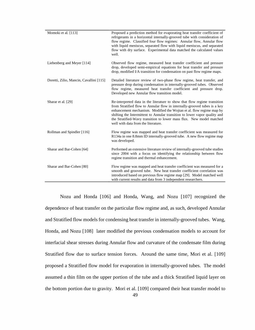
49
Momoki et al. [113] Proposed a prediction method for evaporating heat transfer coefficient of
refrigerants in a horizontal internally-grooved tube with consideration of
flow regime. Classified four flow regimes: Annular flow, Annular flow
with liquid meniscus, separated flow with liquid meniscus, and separated
flow with dry surface. Experimental data matched the calculated values
well.
Liebenberg and Meyer [114] Observed flow regime, measured heat transfer coefficient and pressure
drop, developed semi-empirical equations for heat transfer and pressure
drop, modified I/A transition for condensation on past flow regime maps.
Doretti, Zilio, Mancin, Cavallini [115] Detailed literature review of two-phase flow regime, heat transfer, and
pressure drop during condensation in internally-grooved tubes. Observed
flow regime, measured heat transfer coefficient and pressure drop.
Developed new Annular flow transition model.
Sharar et al. [29] Re-interpreted data in the literature to show that flow regime transition
from Stratified flow to Annular flow in internally-grooved tubes is a key
enhancement mechanism. Modified the Wojtan et al. flow regime map by
shifting the Intermittent to Annular transition to lower vapor quality and
the Stratified-Wavy transition to lower mass flux. New model matched
well with data from the literature.
Rollman and Spindler [116] Flow regime was mapped and heat transfer coefficient was measured for
R134a in one 8.8mm ID internally-grooved tube. A new flow regime map
was developed.
Sharar and Bar-Cohen [64]
Sharar and Bar-Cohen [80]
Performed an extensive literature review of internally-grooved tube studies
since 2004 with a focus on identifying the relationship between flow
regime transition and thermal enhancement.
Flow regime was mapped and heat transfer coefficient was measured for a
smooth and grooved tube. New heat transfer coefficient correlation was
introduced based on previous flow regime map [29]. Model matched well
with current results and data from 3 independent researchers.
Nozu and Honda [106] and Honda, Wang, and Nozu [107] recognized the
dependence of heat transfer on the particular flow regime and, as such, developed Annular
and Stratified flow models for condensing heat transfer in internally-grooved tubes. Wang,
Honda, and Nozu [108] later modified the previous condensation models to account for
interfacial shear stresses during Annular flow and curvature of the condensate film during
Stratified flow due to surface tension forces. Around the same time, Mori et al. [109]
proposed a Stratified flow model for evaporation in internally-grooved tubes. The model
assumed a thin film on the upper portion of the tube and a thick Stratified liquid layer on
the bottom portion due to gravity. Mori et al. [109] compared their heat transfer model to

50
10 correlations available in the literature and experimental data for nine refrigerants and
26 tubes and found that their correlation had the best agreement with a mean absolute error
of 19% for the entire dataset. Momoki et al. [113] later extended the Mori et al. [109]
model and classified four heat transfer regimes: Annular flow, Annular flow with a liquid
meniscus, separated flow with a liquid meniscus, and separated flow with a dry surface,
and proposed empirical correlations for flow regime transitions. They compared their
correlation to experimental data and showed that their regime-informed correlation
outperformed correlations available in the literature.
Honda and Wang [110] modified the condensation Stratified model of Honda,
Wang, and Nozu [107] using the newly-developed Stratified evaporation flow model of
Mori et al. [109] and found reasonable agreement with data in the literature. The agreement
was good for low mass flux and vapor where Stratified flow would be expected but poorly
predicted heat transfer coefficients at high mass flux and vapor quality where Annular flow
would be expected. Additionally, the model did not account for the contribution of
nucleate boiling. In response, Makishi et al. [111] developed a new theoretical model for
Stratified and Annular flow in internally-grooved tubes that considered the effect of
nucleate boiling and forced convection. A modified version of the Kattan et al. [47]
Stratified to Annular transition was used to predict the weighted average heat transfer
coefficient in the intermediate region. The predictions of the new theoretical models and
previously proposed empirical models by Koyama et al. [92], Murata [89], Thome et al.
[91], Cavallini et al. [117], Yun et al. [90], and Mori et al. [109] were compared to available
experimental data for ten internally-grooved tubes and four refrigerants. The model
developed to account for the dependence of flow regime had smaller RMS errors than the

51
empirical models. However, the RMS error of the theoretical model was still fairly high,
at 22.4% to 25.7%.
Finally, Wang et al. [112] modified the previous Makishi et al. [111] model to
account for local heat transfer enhancement due to disturbance waves in internally-grooved
tubes and compared the model to data from the literature. Reasonably good agreement was
found but improvement is needed if they are to be used as a general prediction and design
tool. Specifically, the Wang et al. [112] model uses the dimensionless liquid Froude
number to distinguish between Stratified and Annular flow. Unfortunately, the liquid
Froude number is not sufficient for determining the transition from Stratified to non-
stratified flow [105]. Additionally, the model does not account for Dryout or the effect of
Intermittent flow. Thus, a comprehensive tool similar to the coupled flow regime map and
heat transfer coefficient correlation of Wojtan et al. [30] [31] needs to be developed for
internally-grooved tubes.
In an attempt to answer this call, Liebenberg, Thome, and Meyer [118] observed
and described flow regimes and heat transfer during condensation in horizontal internally-
grooved tubes. They modified the Intermittent to Annular transition on the Thome map
[119] and developed new semi-empirical flow regime based heat transfer and pressure drop
correlations. The modification shifted the Intermittent to Annular transition to lower vapor
quality, a trend apparent from the previous discussion, and greatly improved the predictive
accuracy of condensing flow in internally-grooved tubes. Unfortunately, flow boiling is
not fully analogous to condensation [120] and the flow regime maps and associated heat
transfer models developed for condensation cannot be strictly used for flow boiling. For
example, Liebenberg et al. [114] did not report early transition from Stratified to Annular

52
flow during condensation in internally-grooved tubes. As shown in the preceding
discussion, this is a dominant trend during flow boiling. In addition, nucleate boiling,
Stratified flow with a completely dry upper surface, and dryout do not occur for
condensation.
Thus, research is progressing in the proper direction but, as of yet, a coupled flow
regime map and heat transfer coefficient correlation for flow boiling in internally-grooved
tubes have not been developed. A stronger experimental and theoretical knowledge base
needs to be established, focusing on a more comprehensive understanding of the physical
mechanisms responsible for improved performance in internally-grooved tubes.
3.5 Summary
The preceding has presented a survey of two-phase flow boiling studies in
internally-grooved tubes. The vast majority of the discussion dealt with halogenated fluids
in conventional sized tubes at standard temperature and pressure. Studies of small diameter
tubes, alternative refrigerants, refrigerant/oil mixtures, and elevated reduced pressure were
also considered. Additionally, existing flow regime maps and regime-informed heat
transfer coefficient correlations for internally-grooved tubes were discussed. Through this
process, parametric trends have been identified and goals for the current research effort
have been developed.
In meso-scaled (i.e. “conventional”) internally-grooved tubes, heat transfer
enhancement generally exceeded the area enhancement at low mass flux by factors of 3-7
times a plain tube, but decreased to the area enhancement at high mass flux, yielding
improvement of just 1.3-1.8 times a plain tube. This trend is summarized in Table 3 and
displayed in Figure 9 and Figure 10. It was shown that this performance enhancement at

53
low mass flux can be correlated to early transition to Annular flow in internally-grooved
tubes, for conditions in which smooth tubes were operating in Stratified flow. However,
at high mass flux where the smooth and internally-grooved tubes are both operating in
Annular flow, the enhancement decreased towards the area enhancement. It is argued that
this early transition in internally-grooved tubes is primarily a result of fluid flow redirection
from axial to helical flow (momentum change), augmented by favorable capillary force in
the groove structures. Minor deviations from these parametric trends were observed, such
as enhancement factors larger or smaller than the area ratio at high mass flux, and may be
a result of the particular geometric parameters for the various internally-grooved tubes
tested, turbulence, or nucleate boiling. The trends are less clear for refrigerants and CO2 at
high reduced pressure.
The study of small internally-grooved tubes is still in its infancy and the
experimental studies available are not sufficient to draw clear trends or conclusions
regarding the impact of flow regime on heat transfer performance. Specifically, the
available studies generally tested mass fluxes above 190 kg/m²s where the hypothesized
benefit of early transition from Stratified to Annular flow, with significant enhancement in
the heat transfer coefficient, at low mass flux is not achievable. However, in a fashion
similar to larger diameter tubes, small diameter internally-grooved tubes demonstrated
enhancement close to the internal area ratio at high mass fluxes due to the prevalence of
Intermittent and Annular flow.
The Wojtan et al. [30] flow regime map proved useful for predicting flow regimes
in the smooth channel studies reported above. However, due to observed early transition
to Annular flow at lower mass flux and vapor quality, the Wojtan et al. [30] map, and

54
Mastrullo et al. [54] map, had diminished predictive accuracy for the internally-grooved
tube experimental data. Furthermore, many researchers reported poor agreement with the
most widely used heat transfer coefficient correlations for internally-grooved tubes because
they are either: a) empirical and do not account for flow regime or b) assume a fixed flow
regime, such as Annular flow, and are unable to universally predict heat transfer.
Based on these findings, research objectives and guidelines have been identified
that will provide a more comprehensive understanding of the physical mechanisms
responsible for improved performance in internally-grooved tubes:
a. Concurrent heat transfer and quantitative flow regime data will be collected
over a wide range of operating conditions, particularly low mass flux, to
establish the intrinsic relationship between the dominant flow structure and
thermofluid performance in internally-grooved tubes. Additionally,
comparison to existing correlations, flow regime maps, and smooth tube
data as a means to normalize the results will accompany all experiments to
determine the current state of internally-grooved tube predictive methods.
b. The majority of the studies in the literature relied solely on subjective flow
regime data collection, which calls into question the accuracy of the results.
The current study will focus on an objective Total Internal Reflection (TIR)
flow regime determination method to obtain more accurate data.
c. The study of small diameter internally-grooved tubes has only been a topic
of research since 2006 and, as such, the available experimental data set is
incomplete. Therefore, the current effort aims to test both conventional

55
tubes and extend the small diameter data to a wider range of refrigerants
and operating conditions.
d. The eventual goal of the current research effort is to develop a physics-
based heat transfer model that represents the impact of two-phase flow
structures and is coupled to a reliable flow regime map [105]. Based on the
above research initiatives, a stronger experimental and theoretical
knowledge base will be established, focusing on a more comprehensive
understanding of the physical mechanisms responsible to improved
performance in internally-grooved tubes.
Though outside the scope of the current effort, several additional conclusions and
recommendations for future internally-grooved tube research have been identified based
on the preceding literature review and analysis:
a. It is not entirely clear what impact operation of refrigerants and CO2 at high
reduced pressure has on flow regimes and heat transfer in internally-
grooved tubes. Future studies should be conducted with a focus on items
‘a’ and ‘b’ above.
b. Researchers have observed performance discrepancies for identical test
conditions but variable tube groove parameters. Therefore, a more
systematic study of the effect of tube diameter, fin shape, fin height, number
of fins, helix and apex angle, and ratio of relevant parameters needs to be
undertaken to determine the relationship between these parameters, flow
regime, and thermofluid performance, and what constitutes a geometrically-
optimum tube for given operating conditions.

56
Greater detail on the analytical and experimental research plan, including specifics
on the breadth of work necessary to achieve items ‘a’ through ‘d’ above, are described in
the following chapters.

57
Chapter 4: New Flow Regime Map and Heat Transfer
Coefficient Correlation for Internally-Grooved Tubes
Heat transfer enhancement in internally-grooved tubes is related to early transition
to Annular flow at relatively low mass flux and vapor quality, where a comparable smooth
tube is expected to operate in Stratified or Intermittent flow. As such, the capability to
accurately predict this early transition to Annular flow for a range of tube diameters is
critical to predicting the improved performance in internally-grooved tubes. As shown in
the previous chapter, the original formulations by Wojtan et al. [30] for transition from
Intermittent to Annular and Stratified to Annular flow are adequate for predicting flow
regime in smooth channels for a range of fluids and operating conditions, however, they
are not sufficient for predicting flow regimes in internally-grooved tubes. Therefore, this
chapter gives a description of the original Wojtan et al. [30] [31] formulation and outlines
current modifications to the existing flow regime map and regime-based heat transfer
coefficient correlation to better reflect the trends described in Chapter 3. Lastly, the new
model is simulated through a range of operating conditions to verify that it accurately
captures the trends previously described, namely 3-7x improvement at low-to-moderate
mass flux.
4.1 Taitel-Dukler [46] Annular Transition Criteria
The Wojtan et al. flow regime map [30] is a modification of the Taitel-Dukler [46]
flow regime map. Thus, understanding the Annular flow transition mechanisms outlined
by Taitel-Dukler [46] is a logical starting point for understanding the Wojtan et al. [30]
flow regime map. Taitel-Dukler [46] expressed the Stratified to Annular transition in terms

58
of inertial effects using two-phase non-dimensional groupings. As shown in Figure 15, the
transition to Annular flow can be described using the modified Froude number (F), non-
dimensional Z parameter (Z), and non-dimensional liquid height (hL/D), where hL is the
Stratified liquid height and D is the channel diameter. The Froude number and Z parameter
represent transition ‘F’ and transition ‘Z’ on Figure 15, respectively.
Figure 15: Generalized transition boundaries in Taitel-Dukler model (adapted from [46])
The first inertial effect to consider, as described by the Froude number, is the
stability of the Stratified flow due to the Kelvin-Helmholtz instability. Assuming a
stationary wave on the Stratified liquid interface, two forces can be identified: gravity force
tends to flatten the wave and stabilize the Stratified configuration while the Bernoulli force,
due to the increased gas velocity and associated pressure decrease above the interface,
tends to increase the wave amplitude. If the Bernoulli force is large enough to overcome
the gravity force, the wave will wet the dry upper surface of the channel. A force balance
results in a dimensionless Froude number modified by the density ratio as shown in
Equation (3):
hL/D
F o
r Z
0 0.2 0.4 0.6 0.8 1.010-3
10-2
10-1
100
101
Z
F

59
F = (ρg
ρL − ρg
)
1/2ugs
√Dgcosβ (3)
where ρg is the vapor density, ρL is the liquid density, ugs is the superficial gas velocity, D
is the channel diameter, g is the acceleration of gravity, and β is the tube inclination.
The second transition criterion is attributed to the impingement of liquid droplets
on the top surface, which are torn away from the Stratified liquid-vapor interface. In this
case, transition to Annular flow will occur when liquid droplets have enough kinetic energy
to reach the top of the channel. Calculation of the liquid droplet trajectory is related to the
maximum turbulent velocity fluctuations as estimated by Barnea et al. [121]. The criterion
for Annular flow becomes:
uL2 =
gD (1 −hL
D) cosβ
fL
(4)
where uL2 is the liquid velocity and fL is the liquid friction factor. This transition criterion
can be represented in dimensionless form as the Z parameter:
Z =(dp/dx)Ls
ρLgcosβ (5)
where (dp/dx)Ls is the pressure drop when the tube is completely filled with liquid. The
non-dimensional transition criteria can also be expressed in terms of superficial liquid and
vapor velocities.
The full description of the sequence of tests for iteratively calculating flow regime
for the Taitel-Dukler maps is not included here, for the sake of brevity, but please refer to
[46] for a more comprehensive explanation.

60
4.2 Traditional Wojtan et al. [30] Flow Regime Map for Smooth Tubes
The Taitel-Dukler [46] map requires complex calculations (and an iterative
process) and is not coupled to a reliable flow regime based heat transfer model. This limits
its practical applicability. The Wojtan et al. [30] flow regime map, on the other hand, can
be implemented with simple calculations and has an accompanying comprehensive flow
pattern based heat transfer model; more detail on the Wojtan et al. [31] regime based heat
transfer model will be described in Section 4.4. For these perceived benefits, the Wojtan
et al. [30] map for smooth tubes (and heat transfer coefficient correlation [31]) will be used
as a starting point for analytically describing and mapping early flow regime transition to
Annular flow in internally-grooved tubes. For the sake of completeness, the entire Wojtan
et al. [30] flow regime transition criteria will be described below. Refer to Figure 16 for a
graphical representation of the original smooth tube Wojtan et al. [30] flow regime map.
Figure 16: Traditional smooth tube Wojtan et al. [30] diabatic flow regime map for evaporation of
R134a at -15ºC in a 9mm smooth tube with a heat flux of 4 kW/m²
As shown on Figure 16, the Wojtan et al. [30] map consists of five governing
equations to represent the loci of flow regime transition; Gstrat, Gwavy, xIA, Gdryout, and
0
100
200
300
400
500
0 0.1 0.2 0.3 0.4 0.5 0.6 0.7 0.8 0.9 1
G (
kg/m
²s)
x
Stratified
Intermittent
Annular
Mist
Dryout
Slug
Slug and
Stratified-
Wavy Stratified-Wavy
𝐆𝐬𝐭𝐫𝐚𝐭
𝐆𝐰𝐚𝐯𝐲
𝐱𝐈𝐀
𝐆𝐝𝐫𝐲𝐨𝐮𝐭
𝐆𝐦𝐢𝐬𝐭

61
Gmist. In order to calculate these transition curves the following three dimensionless
geometric variables must first be defined:
hLD = 0.5 (1 − cos (2π − θdry
2))
(6)
AVD =Aε
D2
(7)
ALD =A(1 − ε)
D2 (8)
As shown in Figure 17, hLD is the dimensionless vertical height of the liquid, A is
the total cross-sectional area of the tube, AVD is the dimensionless cross-sectional area
occupied by the vapor phase, ALD is the dimensionless cross-sectional area occupied by the
liquid, and D is the internal tube diameter.
Figure 17: Two-phase Stratified flow cross-section (adapted from [30])
ɛ is the void fraction calculated using the Steiner version of the Rouhani-Axelsson
drift flux model for horizontal tubes [122]. This drift flux model, as opposed to the method
employed by Taitel-Dukler [46], is easy to implement and provides void fraction as a
D
hLDALD
AVD
θstrat
θwet
Vapor
Liquid

62
function of mass flux and vapor quality. The applicability of this model was proven by
Wojtan et al. [123] by optically measuring dynamic void fractions in Stratified types of
flow with R-22 and R-410A as the working fluids. θstrat is an approximation of the
Stratified angle as described by Biberg [124] and θwet is simply θstrat-2π. These terms
can be directly evaluated as:
ε =x
ρV
[(1 + 0.12(1 − x)) (x
ρV
+1 − x
ρL
) +1.18(1 − x)[gσ(ρL − ρV)]0.25
GρL0.5 ]
−1
(9)
θstrat = 2π − 2 π(1 − ε)
+ (3π
2)
13
[1 − 2(1 − ε) + (1 − ε)13 − ε
13
−1
200(1 − ε)ε[1 − 2(1 − ε)][1 + 4((1 − ε)2 + ε2]]
(10)
where x is the vapor quality, G is the mass flux, σ is the fluid surface tension, g is
gravitational acceleration, ρV is the vapor density, and ρL is the liquid density.
After the geometric parameters have been calculated, the Stratified-Wavy to
Intermittent/Annular transition curve (labeled as Gwavy on Figure 16) can be calculated
from the following equation:
Gwavy = 16AVD
3 gDρLρV
x2π2(1 − (2hLD − 1)2)0.5× [
π2
25hLD2 × (
We
Fr)
L
−1
+ 1]
0.5
+ 50 (11)
where Gwavy is the mass flux at which transition occurs, We is the liquid Weber number,
and Fr is the liquid Froude number. It’s interesting to note that the Weber number is a
measure of the relative importance of a fluid’s inertia to its surface tension and is useful
for analyzing the formation of droplets in multiphase flows. Additionally, the Froude

63
number is defined as the ratio of a body’s inertia to gravity forces and, in two-phase flows,
is useful for describing wave formation. Thus, the physical mechanisms described by the
Wojtan et al. [30] Gwavy transition from Stratified to Annular flow are consistent with those
described by Taitel-Dukler and outlined in Section 4.1 above.
The Stratified to Stratified-Wavy transition (labeled as Gstrat on Figure 16) is
calculated from:
Gstrat = [226.32ALDAVD
2 ρv(ρL−ρv)μLg
x2(1−x)π3 ]
1
3
(12)
The Intermittent to Annular transition (labeled as xIA on Figure 16) is calculated
from:
xIA = [0.341
0.875 (ρV
ρL)
−1
1.75(
μL
μV)
−1
7] + 1
−1
(13)
The Annular to Dryout and Dryout to Mist (labeled as Gdryout and Gmist on Figure
16, respectively) are empirically-modified from the dryout inception-completion model of
Mori et al. [125]:
Gdryout = [1
0.235(ln (
0.58
x) + 0.52) (
D
ρvσ)
−0.17
× (1
gDρv(ρL − ρv))
−0.37
(ρv
ρL
)−0.25
(q
qcrit
)−0.70
]
0.926
(14)
Gmist = [1
0.0058(ln (
0.61
x) + 0.57) (
D
ρvσ)
−0.38
× (1
gDρv(ρL − ρv))
−0.15
(ρv
ρL
)0.09
(q
qcrit
)−0.27
]
0.943
(15)
where q is the applied heat flux (at the inside surface of the tube) and qcrit is the critical
heat flux as described by Kutateladze [126]:

64
qcrit = 0.131ρv0.5hLV[g(ρL − ρv)σ]0.25
(16)
where hLV is the latent heat of vaporization.
Once the main transition lines are calculated, further subdivisions at low vapor
quality and high vapor quality, respectively, are made to better predict trends described by
Wojtan et al. [30]. The subdivisions at low vapor quality are described below and shown
on Figure 16:
a. If G > Gwavy(xIA) and < Gwavy(x) , the flow regime becomes Slug.
b. If Gstrat < G < Gwavy(xIA) and x < xIA, the flow regime becomes Slug and
Stratified-Wavy.
c. If Gstrat < G < Gwavy(xIA) and x ≥ xIA, the flow regime is the Stratified-
Wavy zone.
d. If x < xIA, Gstrat = Gstrat(xIA).
The subdivisions to describe dryout and mist conditions at high vapor quality are
as follows:
a. If Gstrat(x) ≥ Gdryout(x), then Gdryout(x) = Gstrat(x).
b. If Gwavy(x) ≥ Gdryout(x), then Gdryout(x) = Gwavy(x).
c. If Gdryout(x) = Gmist(x) (which is possible at low heat flux and high mass
velocity) then Gdryout(x) = Gmist(x).
4.3 Modified Sharar et al. [29] Flow Regime Map for Internally-Grooved Tubes
As described in great detail in Chapter 2 and Chapter 3, the Wojtan et al. [30] flow
regime methodology works particularly well for predicting refrigerant evaporation in
conventionally-size smooth tubes. However, as evident by the early flow regime

65
transitions in internally-grooved tubes and the efforts to modify existing flow regime maps
to account for these variations [111] [118], smooth tube flow regime maps do not
accurately predict flow regimes in internally-grooved tubes. In addition to the inertial and
surface tension effects discussed above, it is suggested in the literature that the capillary
force in the groove structures [111] [110] [84], as well as fluid flow redirection from an
axial direction to a direction following the helix angle of the groove (momentum change)
[27], play a favorable role in transitioning from Stratified and Intermittent flow to Annular
flow.
In order to better capture these trends for evaporative two-phase flow, Sharar et al.
[29] recently modified the existing Wojtan et al. [30] flow regime map by adopting the
Liebenberg et al. [118] and Liebenberg and Meyer [114] Intermittent to Annular transition
criteria and modifying the existing Stratified to Annular transition. The modified
Intermittent to Annular transition is defined by:
xIA = [C (ρL
ρV)
0.5
(μV
μL)
0.1
]1/0.9
+ 1
−1
(17)
where μL is the liquid viscosity, μV is the vapor viscosity, ρL is the liquid density, ρV is the
vapor density, and C is the transition coefficient. For smooth tubes, C=0.3218 and for
internally-grooved tubes C=0.6678 [114]. The modified Stratified-Wavy to Annular
transition was defined by Sharar, Jankowski, and Bar-Cohen [29]:
Gwavy IG = 16AVD
3 gDρLρV
x2π2(1−(2hLD−1)2)0.5 × [π2
25hLD2 × (
We
Fr)
L
−1
+ 1]0.5
− 15 (18)
where Gwavy IG is the mass flux at which transition occurs, AVD is the dimensionless cross-
sectional area occupied by the vapor phase, g is gravitational acceleration, D is the internal
tube diameter, x is the vapor quality, hLD is the dimensionless vertical height of the liquid,

66
We is the liquid Weber number, and Fr is the liquid Froude number. In practice, Equations
(17) and (18) replace Equations (11) and (13) in the original formulation; all other
equations remain the same.
Figure 18 shows the original and modified Sharar et al. [29] flow regime maps for
R134a at -15ºC in a 9 mm diameter tube; Figure 18a is the original smooth tube map
proposed by Wojtan et al. [30] and Figure 18b is the modified Sharar et al. [29] flow regime
map for a comparable internally-grooved tube. Both maps define 8 distinct flow regimes:
Stratified, Stratified-Wavy, Slug and Stratified-Wavy, Slug, Intermittent, Annular, Dryout,
and Mist in coordinates of mass flux (G) and quality (x). The modified map reflects early
transition to Annular flow at lower vapor quality and lower mass flux compared to a smooth
tube.
Figure 18: a) Traditional smooth tube Wojtan et al. [30] and b) modified Sharar et al. [29]
internally-grooved tube diabatic flow regime map for evaporation of R134a at -15ºC in 9mm tubes
with a heat flux of 4 kW/m²
4.4 Traditional Wojtan et al. [31] Heat Transfer Coefficient Correlation
The Wojtan et al. [31] heat transfer coefficient correlation will be used as a starting
point for analytically describing enhanced heat transfer in internally-grooved tubes
0
100
200
300
400
500
0 0.1 0.2 0.3 0.4 0.5 0.6 0.7 0.8 0.9 1
G (
kg/m
²s)
x
0
100
200
300
400
500
0 0.1 0.2 0.3 0.4 0.5 0.6 0.7 0.8 0.9 1
G (
kg/m
²s)
x
Stratified
Intermittent
Annular
Mist
Dryout
Slug
Slug and
Stratified-
Wavy Stratified-Wavy
Stratified
Intermittent
Annular
Mist
Dryout Slug
Slug and
Stratified-
Wavy
Stratified-Wavy
a) b)
𝐆𝐬𝐭𝐫𝐚𝐭 𝐆𝐬𝐭𝐫𝐚𝐭
𝐆𝐰𝐚𝐯𝐲 𝐈𝐆
𝐆𝐰𝐚𝐯𝐲
𝐱𝐈𝐀
𝐆𝐝𝐫𝐲𝐨𝐮𝐭 𝐆𝐝𝐫𝐲𝐨𝐮𝐭
𝐆𝐦𝐢𝐬𝐭 𝐆𝐦𝐢𝐬𝐭
𝐱𝐈𝐀 𝐈𝐆

67
associated with early transition to Annular flow. Wojtan et al. [31] modified the regime-
based heat transfer model of Kattan, Thome, and Favrat [62] using the flow regime map
described in Section 4.2 and shown in Figure 16 and Figure 18a. This model improved
heat transfer prediction during Stratified-Wavy flow, and extended the applicability to high
vapor quality and heat flux where Dryout and Mist flow can occur. The model also
considers the effects of flow regime on the Annular film thickness, turbulence, nucleate
boiling, and the dry perimeter during Stratified flows in smooth tubes to calculate the local
heat transfer coefficient.
During Stratified, Stratified-Wavy, and Annular flow with partial dryout, at least a
portion of the tube is cooled by vapor at the top surface. Therefore, they proposed the
following equation to calculate the heat transfer coefficient as the average of the dry and
wet surfaces:
htp =θdryhv+(2π−θdry)hwet
2π (19)
where htp is the two-phase heat transfer coefficient, θdry is the dry angle (from 0 to 2π),
and hv is the heat transfer coefficient associated with vapor flow on the dry perimeter. The
dry perimeter heat transfer coefficient is expressed in terms of the vapor thermal
conductivity, kv, vapor Reynolds number, Rev, and vapor Prandtl number, Prv:
hv = 0.023Rev0.8Prv
0.4 kv
D (20)
hwet is the heat transfer coefficient for the wet perimeter. Wojtan et al. [31] use
an asymptotic model accounting for the effect of convective vaporization and nucleate
boiling:
hwet = [(hcb)3 + (hnb)3]1
3 (21)

68
The convective vaporization heat transfer coefficient, hcb, is calculated based on
the predicted film thickness, δ, fluid thermal conductivity, kL, liquid film Reynolds
number, Reδ, and liquid Prandtl number, PrL:
hcb = 0.0133Reδ0.69PrL
0.4 kL
δ (22)
The nucleate boiling heat transfer coefficient, hnb, is calculated from a slightly
modified version of the Cooper correlation [127] :
hnb = S × 55(Pr)0.12(−logPr)−0.55M−0.5q0.67 (23)
where M is the fluid molar mass, q is the heat flux, and S is a suppression factor of 0.8
proposed by Wojtan et al. [31] to better match their experimental data; the degree of
improvement obtained by applying the suppression factor was not quantified by Wojtan et
al. [31].
The parameter which takes into account the flow regime in Equation (19) is the dry
angle, θdry, as shown schematically in Figure 17; The original formulation by Kattan,
Thome, and Favrat [62] assumed a linear variation in the wetted perimeter between
Stratified and Annular flow. However, Wojtan et al. [31] found that the complexity
resulting from subdivisions of Stratified-Wavy flow regimes requires a different approach
to calculating dry angle.
For Slug, Intermittent, and Annular flow where the entire perimeter of the channel
is covered with a continuous thick or thin layer of liquid, the dry angle is 0:
θdry = 0 (24)
For Stratified-Wavy flow, Wojtan et al. [31] proposed a modified version of the El
Hajal et al. [128] model which used a quadratic interpolation to calculate θdry. An
exponent of 0.61 showed best agreement with the data from Wojtan et al. [31]:

69
θdry = [(Gwavy−G)
(Gwavy−Gstrat)]
0.61
θstrat (25)
where θstrat is an approximation of the stratified angle as described by Biberg [124],
shown in Figure 17, and expressed in Equation (10). Quantitative measures of
‘improvement’ obtained by adopting the new exponent of 0.61 were not provided by
Wojtan et al. [31].
In the Slug and Stratified-Wavy region, it is possible to have both low amplitude
waves with a dry upper surface and liquid Slugs that completely wet all surfaces of the
tube. As vapor quality increases for a fixed mass flux, the frequency of Slugs decreases
and Stratified-Wavy flow becomes the dominant regime. As the vapor quality approaches
xIA, slugs disappear completely [30]. To capture this trend Wojtan et al. [31] proposed the
following dry angle correlation when x < xIA:
θdry =x
xIA[
(Gwavy−G)
(Gwavy−Gstrat)]
0.61
θstrat (26)
Based on the dry angle, the liquid film thickness is calculated using the equation by
El Hajal et al. [128]:
δ =D
2− √(
D
2)
2
−2AL
(2π−θdry)
(27)
When/if Equation (27) gives a value larger than D/2, δ is set to D/2 because a
symmetric film thickness larger than the tube radius is geometrically impossible.
The model of Kattan et al. [62] did not cover Mist flow or Dryout due to a lack of
experimental data at the time. Wojtan et al. [31] collected heat transfer data and modified
the Groeneveld Mist flow correlation [129] which is a modification of the Dougall-

70
Rohsenow Mist flow correlation [130]. The Dougall-Rohsenow Mist flow correlation
[130] takes the form:
hmist = 0.023ReH0.8Prv
0.4 kv
D (28)
where ReH is the homogeneous Reynolds number:
ReH =GD
μv(x +
ρL
ρv(1 − x))
(29)
Groeneveld [129] determined that the homogeneous Reynolds number described
by Dougall-Rohsenow [130] was not consistent with homogenous theory because vapor
and liquid properties were used rather than homogeneous properties. Therefore,
Groeneveld [129] proposed a correction factor, Y, to be used in calculating hmistand
defined it as:
Y = 1 − 0.1 [(ρL
ρv− 1) (1 − x)]
0.4
(30)
Groeneveld [129] used data obtained from experiments with water as the working
fluid at high mass fluxes, >700 kg/m²s, high saturation pressures, >34 bar, and high heat
fluxes, >120 kW/m², to modify Equation (28), using the proposed correction factor, Y, with
an exponent of -1.5, altering the exponents on the Reynolds and Pradtl numbers, and
introducing a vastly lower value of the empirical coefficient to yield:
hmist = 0.00327ReH0.901Prv
1.32Y−1.5 kv
D (31)
Wojtan et al. [31] further modified the empirical coefficients in the Groeneveld
[129] correlation based on their experimental results to yield Equation (32) below.
hmist = 0.0117ReH0.79Prv
1.06Y−1.83 kv
D (32)
Wojtan et al. [31] compared Mist flow heat transfer results for R-22 and R-410A in
a 13.84mm test section with the correlations from Dougall-Rohsenow [130], Groeneveld
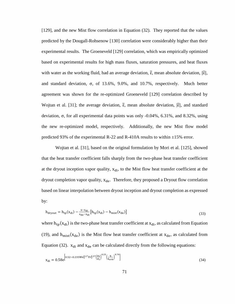
71
[129], and the new Mist flow correlation in Equation (32). They reported that the values
predicted by the Dougall-Rohsenow [130] correlation were considerably higher than their
experimental results. The Groeneveld [129] correlation, which was empirically optimized
based on experimental results for high mass fluxes, saturation pressures, and heat fluxes
with water as the working fluid, had an average deviation, ε, mean absolute deviation, |ε|,
and standard deviation, σ, of 13.6%, 9.0%, and 10.7%, respectively. Much better
agreement was shown for the re-optimized Groeneveld [129] correlation described by
Wojtan et al. [31]; the average deviation, ε, mean absolute deviation, |ε|, and standard
deviation, σ, for all experimental data points was only -0.04%, 6.31%, and 8.32%, using
the new re-optimized model, respectively. Additionally, the new Mist flow model
predicted 93% of the experimental R-22 and R-410A results to within ±15% error.
Wojtan et al. [31], based on the original formulation by Mori et al. [125], showed
that the heat transfer coefficient falls sharply from the two-phase heat transfer coefficient
at the dryout inception vapor quality, xdi, to the Mist flow heat transfer coefficient at the
dryout completion vapor quality, xde. Therefore, they proposed a Dryout flow correlation
based on linear interpolation between dryout inception and dryout completion as expressed
by:
hdryout = htp(xdi) −x−xdi
xde−xdi[htp(xdi) − hmist(xde)] (33)
where htp(xdi) is the two-phase heat transfer coefficient at xdi, as calculated from Equation
(19), and hmist(xde) is the Mist flow heat transfer coefficient at xde, as calculated from
Equation (32). xdi and xde can be calculated directly from the following equations:
xdi = 0.58e[0.52−0.235Wev
0.17Frv0.37(
ρvρL
)0.25
(q
qcrit)
0.70]
(34)

72
xdi = 0.61e[0.57−5.8∙10−3Wev
0.38Frv0.15(
ρvρL
)−0.09
(q
qcrit)
0.27]
(35)
where qcrit is the critical heat flux calculated by Kutateladze [126] in Equation (16).
The regime-informed heat transfer coefficient model described above was
statistically compared to 413 experimental data points for R-22 flow boiling in the
13.84mm smooth tube at mass fluxes from 70 to 700 kg/m²s, heat fluxes from 2 to 57.5
kW/m², and vapor qualities from 0 to xdi. Additionally, 121 data points for Dryout and
Mist flow, x>xdi, were collected to extend the experimental database and heat transfer
methodology to higher vapor qualities and to serve as a basis for model comparison. The
average deviation, ε, mean deviation, ε, and standard deviation, σ, of the data were
calculated based on the original regime-based approach of Kattan, Thome, and Favrat [62]
and the ‘new’ Wojtan et al. [31] model.
For vapor qualities from 0 to xdi, the original Kattan et al. [62] heat transfer
coefficient had an average deviation, ε, mean deviation, |ε|, and standard deviation, σ, of
15.43%, 9.56%, and 14.26%, respectively. For the same conditions, the Wojtan et al. [31]
improved the average deviation, ε, mean deviation, |ε|, and standard deviation, σ, to 2.48%,
6.83%, and 10.39%, respectively. For vapor qualities after dryout, x>xdi, the original
Kattan et al. [62] heat transfer coefficient had an average deviation, ε, mean deviation, |ε|,
and standard deviation, σ, of 913.24%, 725.30%, and 886.80%, respectively. After dryout
(x>xdi), the Wojtan et al. [31] improved the average deviation, ε, mean deviation, |ε|, and
standard deviation, σ, to 91.05%, 116.44%, and 155.59%, respectively. Wojtan et al. [31]
correlated the relatively large, but still markedly improved, predictive error at high vapor
quality in the dryout region to error in experimentally predicting vapor quality. For

73
example, a small error in predicting vapor quality can result in relative errors of 2000%
due to the sharp slope of the heat transfer coefficient in this region [31]. Additional
statistical analysis was provided in the PhD Thesis by Wojtan [131].
To enhance the credibility of the new model, Wojtan et al. [31] compared
independent data from Lallemand et al. [132] for flow boiling of R-22 and R-407C in a
smooth tube at mass fluxes from 100 to 300 kg/m²s and showed equally-good agreement.
Statistical measures were not provided to quantify the agreement between the Lallemand
et al. [132] data and the Wojtan et al. [31] model. Additionally, Chapter 2 (Figure 6)
provides an additional qualitative example of the validity of the Wojtan et al. [30] flow
regime map and associate heat transfer coefficient correlation [31] with more recent data
from Filho and Jabardo [38].
4.5 Modified Heat Transfer Coefficient Correlation
In the current study, the Wojtan et al. [31] heat transfer coefficient described in
Section 4.4 is modified to represent improved performance in internally-grooved tubes,
particularly at low mass flux. A portion of this enhancement will originate from Equation
(25) and Equation (26) whereby a modified (reduced) Stratified-Wavy to Annular
transition, Gwavy IG, and Intermittent to Annular transition, xIA IG, will result in a smaller
dry angle, θdry, and a larger two-phase heat transfer coefficient, htp, in Equation (19).
The remaining enhancement derives from an internally-grooved tube enhancement factor
for single-phase turbulent flow, Erb, (developed by Ravigururajan and Bergles [28]) and
an empirically derived enhancement factor introduced by Thome et al. [91], Emf, that
accounts for the effects of film flow and the Gregorig effect. The turbulent enhancement
factor, Erb, can be expressed as:

74
Erb = 1 + [2.64Reδ0.036PrL
−0.024 (ef
df)
0.212
(pf
df)
−0.21
(αf
90°)
0.29
]7
1/7
(36)
where ef is the groove height, df is the nominal inside diameter at the fin base, pf is the
axial pitch from groove to groove, and αf is the helix angle of the grooves. With this
modification, hwet from Equation (21) and Equation (19) becomes:
hwet = Emf[(Erbhcb)3 + (hnb)3]1
3 (37)
where Emf is an additional enhancement factor proposed by Thome et al. [91] that accounts
for the effects of film flow and the Gregorig effect. The Gregorig effect enhances
evaporation by drawing liquid from the microfin tips towards the base as described by
Carey [34]. The enhancement factor, Emf, takes the form:
Emf = 1.89 (m
mref)
2
− 3.7 (m
mref) + 3.02 (38)
where mref is the maximum mass flux tested (500 kg/m²s). This was introduced to non-
dimensionalize the expression.
Ravigururajan and Bergles [28] developed their model based on a broad collection
of data from the literature. The data covered a wide range of Reynolds numbers (from
6000 to 440000), Prandtl numbers (from 0.66 to 37.6), and tube variables. Specifically, ef
df
values from 0.01 to 0.218, pf
df values from 0.1 to 17.81, and
αf
90° values from 0.27 to 1 were
used. Semi-circular, wire coils, rectangular, and triangular ‘fin’ shapes were compared to
the model. The Ravigururajan and Bergles [28] correlation was found to accurately predict
99% of the data from the literature to within ±50% accuracy.
Ravigururajan and Bergles [28] performed independent experiments to further
determine the applicability of the correlation. Water or air were used as the heat transfer

75
fluids for four commercially available tubes from General Atomic, Wolverine, and Turbo
Refrigerating as well as four wire-coil tubes fabricated by the researchers. The normalized
roughness heights, ef
df, varied from 0.038 to 0.127, the normalized pitch,
pf
df, ranged from
0.169 to 1.05, and the normalized helix angle, αf
90°, ranged from 0.33 to 0.91. Reynolds
numbers from 150 to 20000 were tested. The new correlation was ‘in excellent agreement’
with the heat transfer data for both air and water, although quantitative measures of
statistical fit were not provided.
As shown in Equation (36) and also reported by Ravigururajan and Bergles [28],
the increase in the augmentation was predominantly controlled by the tube design rather
than the cooling liquid and flow parameters. This is evidenced by the very low powers of
Re and Pr. This suggests that this correlation should generally work well for fluids and
flowrates outside the range experimentally validated by Ravigururajan and Bergles [28].
Thome et al. [91] validated the use of the Emf correlation with a statistical
comparison of 362 local heat transfer coefficients for R-134a and R-123 with vapor
qualities from 0.15 to 0.85. The standard deviation, mean deviation, and average deviation
for the R-134a data was 18.5%, 12.8%, and 2.0%, respectively. The standard deviation,
mean deviation, and average deviation for the R-123 data was 12.9%, 11.8%, and 6.4%.
The authors indicated that future work should involve validation for a wider range of tube
geometries and fluids.
4.6 Model Simulation
As previously described, internally-grooved tubes have shown heat transfer
enhancement ratios as high as 6 to 7 times that of smooth tubes at low mass velocities and

76
improvement equal to, or slightly greater than, the internal area ratio, 1.3-1.8x that of a
smooth tube, at high mass velocities [26] [17]. The goal of this section is to perform
simulations of the above flow regime based heat transfer coefficient model with a range of
operating conditions to determine if the updated model is capable of capturing these trends.
This also provides examples to demonstrate how the physical model works.
Figure 19 and Figure 20 show flow regime maps and heat transfer coefficient
modeling results for 8.84mm inside diameter smooth and internally-grooved tubes for
HFE-7100 at 61°C with mass fluxes of 25, 50, 100, 150, 200, 250, and 300 kg/m²s and a
heat flux of 4kW/m². Figure 19a and Figure 19b show the traditional Wojtan et al. [30]
flow regime map and corresponding heat transfer coefficient [31], respectively,
superimposed on the locus of mass fluxes described above. Figure 20a and Figure 20b
show the modified Sharar et al. [29] flow regime map and corresponding heat transfer
coefficient described in Section 4.3 and Section 4.5, respectively, superimposed with the
same mass fluxes. The internally-grooved tube parameters used for this simulation are for
the Wieland Cuprofin copper tube S2AD-952 described in Table 2; the simulated tube has
60-0.2mm tall fins with a helix angle of 18° and an area enhancement of 1.52.
As shown in Figure 19a and Figure 20a, the smooth and internally-grooved tube
are predicted to operate in Slug, Intermittent, and Annular flow (before dryout occurs) for
mass fluxes of 200, 250, and 300 kg/m²s. In these cases, the dry angle (θdry) is zero and
the film thickness in Equation (22) is decreasing as the vapor quality increases. The result,
as shown in Figure 19b and Figure 20b, is a monotonically increasing heat transfer
coefficient with increasing vapor quality and internally-grooved tube enhancement ratios,
(i.e. the internally-grooved tube heat transfer coefficient divided by the smooth tube heat
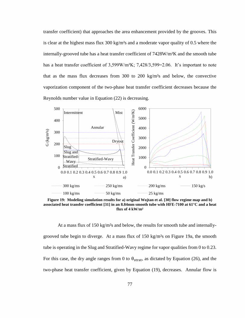
77
transfer coefficient) that approaches the area enhancement provided by the grooves. This
is clear at the highest mass flux 300 kg/m²s and a moderate vapor quality of 0.5 where the
internally-grooved tube has a heat transfer coefficient of 7428W/m²K and the smooth tube
has a heat transfer coefficient of 3,599W/m²K; 7,428/3,599=2.06. It’s important to note
that as the mass flux decreases from 300 to 200 kg/m²s and below, the convective
vaporization component of the two-phase heat transfer coefficient decreases because the
Reynolds number value in Equation (22) is decreasing.
Figure 19: Modeling simulation results for a) original Wojtan et al. [30] flow regime map and b)
associated heat transfer coefficient [31] in an 8.84mm smooth tube with HFE-7100 at 61°C and a heat
flux of 4 kW/m²
At a mass flux of 150 kg/m²s and below, the results for smooth tube and internally-
grooved tube begin to diverge. At a mass flux of 150 kg/m²s on Figure 19a, the smooth
tube is operating in the Slug and Stratified-Wavy regime for vapor qualities from 0 to 0.23.
For this case, the dry angle ranges from 0 to θstrat, as dictated by Equation (26), and the
two-phase heat transfer coefficient, given by Equation (19), decreases. Annular flow is
0
100
200
300
400
500
0.0 0.1 0.2 0.3 0.4 0.5 0.6 0.7 0.8 0.9 1.0
G (
kg/m
²s)
x
0
1000
2000
3000
4000
5000
6000
0.0 0.1 0.2 0.3 0.4 0.5 0.6 0.7 0.8 0.9 1.0
Hea
t T
ransf
er C
oef
fici
ent
(W/m
²K)
x
0100200300400500
0.0 0.1 0.2 0.3 0.4 0.5 0.6 0.7 0.8 0.9 1.0
G (
kg/m
²s)
x
300 kg/ms 250 kg/ms 200 kg/ms 150 kg/s
100 kg/ms 50 kg/ms 25 kg/ms
Stratified
Intermittent Mist
Dryout
Slug
Slug and
Stratified-
Wavy Stratified-Wavy
Annular
a) b)

78
reached after a vapor quality of 0.23 and the dry angle is then zero. At this point, the
smooth tube is operating in Annular flow and the heat transfer coefficient profile begins
increasing monotonically. The internally-grooved tube shows a similar, yet slightly altered
profile. Similar to the smooth tube, the internally-grooved tube begins operating in the
Slug and Stratified-Wavy flow regime, the dry angle is non-zero, and the heat transfer
coefficient remains low. However, because the Intermittent to Annular transition line is
shifted to a lower vapor quality (Equation (17)), the internally-grooved tube reaches
Annular flow at a lower vapor quality of 0.12 in Figure 20a. After this point, it follows a
similar monotonically increasing Annular flow profile to that exhibited by the smooth tube.
Figure 20: Modeling simulation results for a) Modified Sharar et al. [29] internally-grooved tube
flow regime map and b) associated heat transfer coefficient in an 8.84mm internally-grooved tube
with HFE-7100 at 61°C and a heat flux of 4 kW/m²
At a mass flux of 100 kg/m²s, the smooth tube is operating in the Slug and
Stratified-Wavy or Stratified flow regime for all vapor qualities and the internally-grooved
tube begins operating in the Slug and Stratified-Wavy flow regime and transitions to
Annular flow at a vapor quality of 0.25. For the smooth tube, the dry angle ranges from 0
0
100
200
300
400
500
0.0 0.1 0.2 0.3 0.4 0.5 0.6 0.7 0.8 0.9 1.0
G (
kg
/m²s
)
x
0
2000
4000
6000
8000
10000
12000
0.0 0.1 0.2 0.3 0.4 0.5 0.6 0.7 0.8 0.9 1.0
Hea
t T
ran
sfer
Co
effi
cien
t (W
/m²K
)
x
0100200300400500
0.0 0.1 0.2 0.3 0.4 0.5 0.6 0.7 0.8 0.9 1.0
G (
kg
/m²s
)
x
300 kg/ms 250 kg/ms 200 kg/ms 150 kg/s
100 kg/ms 50 kg/ms 25 kg/ms
Stratified
Intermittent Mist
Dryout Slug
Slug and
Stratified-
Wavy Stratified-Wavy
Annular
a) b)
300 kg/m²s 250 kg/m²s 200 kg/m²s 150 kg/m²s
100 kg/m²s 50 kg/m²s 25 kg/m²s

79
to θstrat as dictated by Equation (25) and (26) for all vapor qualities. The result is a
relatively poor, yet slightly increasing, heat transfer coefficient as the vapor quality
increases. Under the same conditions, the internally-grooved tube transitions to Annular
flow and the heat transfer coefficient increases sharply with increasing vapor quality. At a
moderate vapor quality of 0.5 where the internally-grooved tube is operating in Annular
flow (h=4,968W/m²K) and the smooth tube is operating in Stratified-Wavy flow
(h=954W/m²K) the enhancement ratio is 5.2.
The simulation showed similar performance enhancement in the internally-grooved
tube at a mass flux of 50 kg/m²s. As shown in Figure 19a, the smooth tube is operating in
the Slug and Stratified-Wavy or Stratified flow regime. The internally-grooved tube,
shown in Figure 20a, begins operating in the Slug and Stratified-Wavy flow regime at low
vapor quality and approaches Annular flow at higher vapor qualities. The resulting smooth
tube heat transfer coefficient remains low due to Stratified flow, and a large dry angle in
Equation (19), and reaches a value of 320W/m²K at a vapor quality of 0.5. However,
because the internally-grooved tube flow regime is approaching Annular flow, the dry
angle decreases with increasing vapor quality and the heat transfer coefficient increases to
a value of 1,737W/m²K at the same vapor quality. This represents an enhancement ratio
of 5.4.
At the lowest vapor quality modeled, 25 kg/m²s, both the smooth tube and
internally-grooved tube are operating exclusively in the Stratified and Stratified-Wavy
flow regimes. In this case, the dry angle is always between the stratified angle, Equation
(10), and θdry as described by Equation (25). The combined effect of a poor convective
vaporization term (Equation (22)) and a large dry angle is a poor heat transfer coefficient,

80
as calculated by Equation (19). For a mass flux of 25 kg/m²s, the smooth tube had a heat
transfer coefficient of 207W/m²K and the internally-grooved tube simulation showed a heat
transfer coefficient of 553W/m²K. The enhancement ratio in this case reduced to 2.6, again
approaching the area enhancement provided by the grooves.
Figure 21 shows a graphical summary of the enhancement ratio vs mass flux based
on Figure 19, Figure 20, and the analysis above. The green dashed line represents the
predicted enhancement ratios for a vapor quality of 0.5 and plotted as a function of mass
flux; again, the enhancement ratio is defined as the internally-grooved tube heat transfer
coefficient divided by the smooth tube heat transfer coefficient. The solid red line is the
area enhancement of the internally-grooved tube.
Figure 21: Simulated results comparing enhancement ratio vs mass flux for 8.84mm smooth and
internally-grooved tubes with HFE-7100 at 61°C and a heat flux of 4 kW/m² as shown in Figure 19
and Figure 20
The figure shows heat transfer improvement approaching the area enhancement of
1.52 at sufficiently low mass flux, where both tubes were operating in Stratified or
0
1
2
3
4
5
6
7
8
0 100 200 300 400
Enhan
cem
ent
Rat
io
G (kg/m²s)
Enhancement Ratio Area Enhancement

81
Stratified-Wavy flow, and at high mass flux, where both tubes are predicted to operate in
the Slug, Intermittent, or Annular flow regimes. Large enhancement (6 to 7x) was
predicted at low-to-intermediate mass fluxes where the smooth tube was operating in
Stratified flow and the internally-grooved tube is operating in Annular flow. The practical
benefit of operating at low mass flux, where the enhancement is predicted to be 6-7x, is the
reduction in pumping power associated with this operating condition. These trends are
consistent with those described earlier, in Chapter 1 and Chapter 3, and indicate that the
new flow regime map and associated heat transfer coefficient correlation likely capture the
physical mechanisms responsible for enhancement in internally-grooved tubes.
Figure 22 shows a more detailed summary of the enhancement mechanisms
responsible for improved performance in internally-grooved tubes. As shown, the
Ravigururajan and Bergles [28] turbulent enhancement does not vary significantly over the
range of mass fluxes considered; the enhancement factor is 1.426 at a mass flux of 400
kg/m²s and 1.271 at a mass flux of 10 kg/m²s. The Thome et al. [91] enhancement factor,
on the other hand, increases from 1.269 at a mass flux of 400 kg/m²s to 2.947 at a mass
flux of 10 kg/m²s. As shown in Figure 22, the enhancement ratio has the same slope as the
Thome et al. [91] enhancement factor for mass fluxes ranging from 400 kg/m²s to
approximately 150 kg/m²s where Slug, Intermittent, and Annular flow are the dominant
flow regimes for both the smooth and internally-grooved tubes; please refer to Figure 19
and Figure 20. For this range of mass fluxes, enhancement is dominated by area
enhancement, turbulence (as described by Ravigururajan and Bergles [28]), and the
Gregorig effect/film flow (as described by Thome et al. [91]).

82
At mass fluxes below 150 kg/m²s, the slope and value of the enhancement ratio
significantly increases due to sustained Annular flow in the internally-grooved tube and
transition to Stratified-Wavy flow in the smooth tube. In this case, enhancement is
dominated by the observed/predicted dominance of Annular flow in the grooved tube.
Annular flow results in a dry angle of zero for the internally-grooved tube and Stratified
flow results in a dry angle between 0 and 2π for the smooth tube; again, please refer to
Figure 19 and Figure 20. At low mass flux, the total enhancement is less than the
component of the Thome et al. [91] enhancement because a large dry angle is predicted in
the internally-grooved tube during Stratified flow. Recall that the Ravigururajan and
Bergles [28] and Thome et al. [91] enhancement factors only contribute to the wet angle
heat transfer coefficient, as shown in Equation (37).
Figure 22: Simulated results comparing enhancement ratio, Emf, and Erb vs mass flux for 8.84mm
smooth and internally-grooved tubes with HFE-7100 at 61°C and a heat flux of 4 kW/m²
4.7 Summary
In this chapter, a new flow regime map and heat transfer coefficient correlation
were developed that consider the impact of the internal grooves on the flow regime and
0
1
2
3
4
5
6
7
8
0 100 200 300 400
Enhan
cem
ent
Rat
io
G (kg/m²s)
Current model area enhancement
Emf Erb
0
1
2
3
4
5
6
7
8
0 100 200 300 400
Enhan
cem
ent
Rat
io
G (kg/m²s)
Enhancement Ratio area enhancement
Emf Erb
Area Enhancement

83
heat transfer enhancement. The existing Wojtan et al. [30] flow regime map was modified
using the Liebenberg et al. [118] and Liebenberg and Meyer [114] Intermittent to Annular
transition and the Sharar, Jankowski, and Bar-Cohen [29] Stratified-Wavy to Annular
transition. Additionally, the Ravigururajan and Bergles [28] turbulence factor and an
empirically derived enhancement factor, introduced by Thome et al. [91], were adopted to
modify the associated heat transfer coefficient correlation. These modifications resulted
in varying the calculated dry perimeter angle, θdry, and represent the physical mechanisms
responsible for enhancement in internally-grooved tubes.
Through analytical modeling simulations, it was shown that heat transfer
enhancement at high mass flux (>150 kg/m²s) is dominated by area enhancement,
turbulence (as described by Ravigururajan and Bergles [28]), and the Gregorig effect/film
flow (as described by Thome et al. [91]). Enhancement of 6-7x at low-to-intermediate
mass flux is dominated by transition to Annular flow in the internally-grooved tube.
Additionally, predicted heat transfer enhancements approach the area enhancement when
the smooth and internally-grooved tubes are operating in the same flow regime; this was
shown at sufficiently low mass flux, where Stratified flow is expected, as well as high mass
flux, where Annular flow is expected.
One motivation for the current research effort is to experimentally validate the peak
enhancement demonstrated in Figure 21 and Figure 22. Clearly, understanding
performance at and near this high enhancement operating space is critical to proper design
and optimization of two-phase systems.

84
Chapter 5: Experimental Setup and Procedures
In the course of this study, the thermofluid characteristics of a series of
experimental tests for single, uniformly heated horizontal internally-grooved tubes and
smooth tubes with various IDs were experimentally studied. Focus was given to collecting
and processing flow regime and heat transfer coefficient data to validate flow regime
transition as a key enhancement mechanism in internally-grooved tubes and validate the
new flow regime map and heat transfer model described in Chapter 4. This chapter
describes the test facility designed and fabricated to collect flow regime data, using a new
Total Internal Reflection method, and heat transfer coefficient data, using infrared
thermography, for two-phase HFE-7100 flow in horizontal 2.62mm - 8.84mm diameter
smooth and internally-grooved tubes with mass fluxes from 25-300 kg/m²s, heat fluxes
from 4-56 kW/m², and exit vapor qualities approaching 1.
The following sections outline the experimental flow loop, tube heating method,
fluid selection, experimental ranges, tube parameters, data acquisition scheme, vapor
quality and heat transfer coefficient calculation, and uncertainty analysis. This approach
is inspired by the tasks and goals set forth in previous chapters.
5.1 Two-Phase Testing Setup
As shown schematically in Figure 23, a test setup was developed to test single- and
two-phase performance in smooth and internally-grooved horizontal tubes with water (for
calibration and system validation purposes) and HFE-7100 as the working fluids. A
custom reservoir and degasser (a) and a Fluid-o-Tech TMFR motor/pump system (b) are
used to store, degas, heat, and pump the fluid during testing. The degasser is necessary to

85
remove dissolved air in the fluid, before two-phase experiments commence, because
dissolved gasses have been shown to affect performance in smooth channels [133]. To the
author’s knowledge, the effect of degassed and gassy fluid on heat transfer in internally-
grooved tubes has not been experimentally explored. The current setup is a closed loop
system to allow degassing of dielectric fluid and prolonged testing, without the possibility
of non-condensible gas entering the system.
Figure 23: Schematic of two-phase flow test setup: a) reservoir and degasser b) Fluid-o-Tech pump c)
Atrato or Kobold flow meter d) control valves e) inline heater f) 0.2m developing flow section g) 0.2m
test tube h) 8cm sight glass (location of high speed flow visualization and TIR method) i) condenser
P) pressure transducers and T) thermocouple probes DP) differential pressure transducer
An Atrato ultrasonic flow meter with ±1.5% absolute reading accuracy and 250:1
turndown ratio (20 mL/min to 5 L/min) was used to measure flow rate for water calibration
tests. Kobold DPM 1153 and 1170 pelton wheel flow sensors with ±1.5% full scale
accuracy and flowrate ranges of 0.24-4.8 GPH and 0.8-30 GPH, respectively, were used to
measure flowrate for HFE-7100 tests (c). It’s interesting to note that the Atrato ultrasonic
flow meter did not work with HFE-7100 due to fluid compressibility and ultrasonic
(b)
(c)
(d)
(e) (f) (h) (g)
(a)
(d) (i)
T T T
T
P
P
DP

86
modulation. Swagelok fluid control valves (d) were used to better control system flowrate
and pressure. An Omegalux inline heater (e) was installed to further preheat and vaporize
the fluid when necessary. A 0.2m-long smooth or – alternatively – an internally-grooved
tube developing flow section (f) was placed directly before a corresponding 0.2m-long test
section (g) and was connected with custom tube fittings made using a FDM Titan rapid
prototyping machine. A custom 0.08m-long Pyrex sight glass (h), with the same ID as the
internally-grooved and smooth tubes, was placed at the exit of the test section (g) to observe
the local flow regime. A parallel plate heat exchanger (i) was used to re-condense the
vapor produced during two-phase operation.
Fluid pressure was measured by two Omega MMG050 pressure transducers (P),
with ±0.05% full scale reading accuracy and 0-50psi pressure limits, after the flowmeter
and before the test section. Pressure drop across the developing flow section, test section,
and 0.08m-long sight glass was measured with a Setra Model 230 wet-to-wet differential
pressure transducer with ±0.25% full scale reading accuracy and 0-25psi differential
pressure limits. The fluid temperature at the inlet and outlet of the test section was
measured by two Special Limits of Error (SLE) Omega Type T thermocouples with ±0.5ºC
accuracy. Similarly, two SLE Type T thermocouples were used to measure the fluid
temperature before the inline heater and after the condenser. An AeroVironment MT30
power supply, capable operating up to 120 V and 330 A, was used to supply electrical
power to the inline heater. Delivered power was measured by a Tektronix TC312 current
probe and Yokogawa 7000924 differential voltage probe. A Tenma 72-6851 power supply
capable of 35V (±0.1% absolute reading) and 10A (±0.2% absolute reading) was used to
heat the test tube and was interfaced with a GPIB for ease of experimentation.

87
The tube outside wall temperature was measured using a FLIR ThermoVisionA40
long wave IR thermal camera (7.5 to 13 μm, ±0.3ºC accuracy [134]) at 14 discrete locations
along the tube and three axial locations (top, side, and bottom), providing 42 discrete
temperature data points. This was accomplished with the use of a custom fabricated 5-inch
long IR mirror, as shown schematically in Figure 24. An IR photograph, taken during
testing of the 2.80mm smooth tube, is shown in Figure 25. The ABS mirror mount was
created using a FDM Titan rapid prototyping machine. Using a CHA E-Beam evaporator,
the mirror surfaces were created by depositing an adhesion layer of 50nm of titanium (Ti),
at a rate of 5Å/s for 100s, followed by 150nm of gold (Au), at a rate of 5Å/s for 300s, on
Pyrex strips that measured 0.1”x1.15”x5”. The IR mirrors were attached to the mirror
mount, metallization side facing towards the camera, using Loctite E-20HP structural
adhesive. Gold is an excellent IR reflector beyond 1.5 μm with reflectance greater than
99% and, unlike aluminum or silver, is resistant to oxidation and degradation over time
[135] [136]. Therefore, gold was an ideal candidate for the current experiments.
Figure 24: Schematic of custom IR mirror setup for measuring temperature on the top, middle, and
side of the test section
ABS 3D
printed IR
mirror
mount
Copper
test
section
To FLIR
A40 IR
camera
Ti-Au
coated
Pyrex IR
mirrors

88
A Keyence VW6000 high speed camera capable of up to 25,000 fps was used to
observe the flow regimes in the sight glass. At the same location, an optical total internal
reflection (TIR) method using a red fiber optic light source [137] was used to observe and
quantify flow regime; more detail will be given in Chapter 6. It is noteworthy to point out
that flow patterns were observed through sight glasses that are smooth rather than
internally-grooved. Nevertheless, they are assumed to be representative of the flow
regimes actually occurring at the internally-grooved tube exit. It is conjectured that the
internally-grooved tube flow structure persists into the sight glass section and experiences
only minor disruptions do to its short length and low 𝐿ℎ/𝐷; the distance from the end of
the test section and the location of the total internal reflection measurement, and high speed
flow visualization, is 0.015m and 0.03m, respectively.
Figure 25: Schematic of custom IR mirror setup for measuring temperature on the top, middle, and
side of the test section, and an IR photograph of the 2.80mm smooth tube during testing
5.2 Tube Heating Method
The smooth and internally-grooved tube diabatic test sections (‘g’ on Figure 23)
were experimentally heated using custom-fabricated thin-film heaters deposited on the
outside of the tubes. To create the heaters, the tubes were coated with 8 μm Parylene-C in
a Specialty Coating Systems PDS2010 coating tool. This provided a dielectric layer to
prevent electrical energy from shorting through the highly conductive copper tube. Next,

89
the resistor material, consisting of 12,000 Å of Titanium at a rate of 4 Å/s and 2,000 Å of
Platinum at a rate of 2 Å/s, was deposited in a CHA E-beam evaporator using a rotating
stepper motor assembly. These thicknesses were chosen to provide an appropriate
resistance, ~5-20Ω, for electrically heating the tube; details on these values are provided in
Appendix A. Then, copper electrical leads were attached to the metalized tube with EPO-
TEK H20E silver-filled epoxy. Finally, the entire assembly was sprayed with Boron
Nitride to provide a uniform emissivity. During testing, the thin film resistor was heated
with a TENMA 72-6851 DC power supply. Figure 26 shows a photograph of the smooth
tube before attaching the electrical leads and spraying with Boron Nitride. Boron Nitride
emissivity was assumed to be 0.96 for all test conditions [138]. Please refer to Appendix
A for a discussion of alternative tube heating methods considers as well as an attempt to
make thin film resistors using atomic layer deposition (ALD).
Figure 26: Photograph of a smooth tube coated with a thin-film heater
5.3 Fluid Selection
As discussed in Chapter 2 and Chapter 4, the Taitel-Dukler [46], original Wojtan
et al. [30], and modified Sharar et al. [29] maps were developed using phenomenological
models and, as such, are amenable to general use and applicable to a variety of fluids and
flow conditions. From this perspective, any fluid could theoretically be used in the
following tests and extrapolated to other conditions. However, the fluid selected should
8 μm Parylene-C Cu tube 1.2 μm Ti and 0.2 μm Pt

90
have properties close to the fluid used in other internally-grooved tube studies [110] [111]
[66] [77] so that direct comparison can be made. Furthermore, selecting a fluid with
properties similar to the fluids used to develop semi-empirical flow regime [47] [48] [49]
[50] [30] maps provides the added benefit of a large database of smooth tube data for
comparison. Additional considerations when choosing a fluid are saturation temperature,
saturation pressure, and latent heat of vaporization. If the fluid boils at a relatively high
saturation temperature in atmospheric pressure, the vapor can be condensed by an air- or
water-cooled condenser, as in the schematic shown in Figure 23, and a refrigeration
compression loop is not necessary. Furthermore, if the fluid has a low to moderate latent
heat of vaporization, less heat will be required to reach the desired vapor quality; this
should be considered beneficial from an experimental standpoint.
Table 7 summarizes the fluids and properties used in the empirical flow regime
maps discussed in Chapter 2 and Chapter 4, [47] [48] [49] [50] [30], along with several
candidate fluids, FC-72, HFE-7100, and water. Water, which is renowned as a thermal
management fluid, has dramatically different properties than the refrigerants and dielectric
liquids and is not suitable as a heat transfer fluid for the current study. As shown in Table
7, HFE-7100 has fluid properties similar to the fluids used to define the empirical flow
regime maps and similar to the studies outlined in the literature review (most of which used
R-134a). Additionally, HFE-7100 has a moderate boiling point (61˚C) at ambient pressure
and a relatively low latent heat of vaporization (112 kJ/kg). Therefore, the current research
used degassed HFE-7100 as the working fluid. Fluid properties for FC-72 and HFE-7100
were not included in the table for pressure of 900 kPa (0.9 MPa) because properties were
not available. Additionally, it should be noted that there appears to be some inconsistencies

91
in reported properties for HFE-7100, FC-72 and other 3M Novec fluids [139]; this will
inevitably lead to uncertainty in measurement and modeling results. Unfortunately, this
uncertainty cannot be quantified at this time. Efforts should be made to better characterize
these fluids.
Table 7: Comparison of fluids (and properties) used for empirically fitted flow regime maps and
candidate fluids Boiling Point
(˚C)
ρl (kg/m³) ρg (kg/m³) σ (mN/m) µl (µPa-s) µg (µPa-s) hlg (kJ/kg)
Fluid 0.1
MPa
0.9
MPa
0.1
MPa
0.9
MPa
0.1
MPa
0.9
MPa
0.1
MPa
0.9
MPa
0.1
MPa
0.9
MPa
0.1
MPa
0.9
MPa
0.1
MPa
0.9
MPa
R-22 -41 20 1410 1211 4.64 38.05 18.1 8.8 347 174 9.68 12.2 234 188
R-134a -26 36 1377 1165 5.19 44.08 15.5 6.7 380 171 9.76 12.2 217 168
R-410a -52 4 1361 1154 4.12 33.82 17.8 8.5 387 162 9.89 12.8 272 216
FC-72 56 N/A 1680 N/A 13.4 N/A 10 N/A 262 N/A 12.1 N/A 88 N/A
HFE-7100 61 N/A 1370 N/A 9.87 N/A 14 N/A 275 N/A 11.3 N/A 112 N/A
Water 100 175 958 891 0.59 4.653 58.9 43.2 283 154 12.3 14.9 2257 2030
5.4 Experimental Ranges
Wieland, a leading manufacturer of smooth and internally-grooved refrigeration
tubes, was contacted, informed of the current research initiative, and agreed to provide
smooth and internally-grooved copper tubes. They provided six, 1 meter long lengths of
various internally-grooved and smooth tubes. Additional smooth tubes with comparable
inside diameters and wall thicknesses were purchased from McMaster-Carr. Table 8
outlines the parameters of interest for the smooth and internally-grooved tubes used for the
current study. As shown, tube inside diameters ranged from 2.62mm to 8.84mm, tube wall
thicknesses range from 0.19 to 0.9mm, number of fins ranges from 36 to 60, fin height
ranges from 0.12 to 0.2mm, fin base ranges from approximately 0.12 to 0.25mm, and helix
angles range from 10˚ to 18˚. All the internally-grooved tubes have trapezoidal fin profiles
and surface enhancements between 152-160% compared to smooth tube equivalents.
18cm-long heated tube lengths of the 2.62mm, 4.54mm, and 8.84mm ID tubes were
used to simulate channel lengths typical in an IGBT cold plate, thus creating the cold plate
‘unit cell’. These tube diameters cover the range of past research, for comparison purposes,

92
and also smaller sized channels that approach mini- and microchannels to explore the size
effects in internally-grooved tubes. It is unclear what effect heated length has on internally-
grooved tube performance, however, this aspect is outside the scope of the current effort.
Table 8: Geometric parameters of internally-grooved and smooth tubes for the current study
Manufacturer Type Inside
Diameter
(mm)
Wall
thickness
(mm)
#
fins
Fin
height
(mm)
Fin base
(mm)
Helix
angle α
(˚)
Surface
enhancement
(%)
Wieland IG 2.62 0.19 36 0.12 0.12 10 160
McMaster
Smooth 2.8 .9 N/A N/A N/A N/A N/A
Wieland IG 4.54 0.23 40 0.15 0.20 18 152
McMaster smooth 4.54 0.23 N/A N/A N/A N/A N/A
Wieland IG 8.84 0.34 60 0.2 0.25 18 152
Wieland smooth 8.84 0.34 N/A N/A N/A N/A N/A
Nine different flowrates were tested (25, 50, 75, 100, 125, 150, 175, 200, and 300
kg/m²s) for the 8.84mm ID tubes, eight flowrates were tested for the 4.54mm tubes (50-
300 kg/m²s), and seven flowrates were tested for the 2.62 – 2.8mm tubes (75-300 kg/m²s).
This represents Reynolds numbers ranging from 640 to 12000; this is based on average
liquid/vapor properties, superficial velocities, and vapor qualities from 0 to 1. The Kobold
flow meters used in the current study could not accurately measure flowrates below these
lower bounds. Six different tube heat fluxes were tested; 4, 9, 18, 28, 40, and 56 kW/m².
Vapor qualities ranging from 0 to 1 were tested. These mass fluxes centered around regions
near the Stratified/Annular, Stratified/Intermittent, and Intermittent/Annular transitions
because these are the regions where internally-grooved tubes have demonstrated heat
transfer improvement that can be explained by flow regime transition. However, data well
within a specified flow regime (away from the transitions, as is the case with mass fluxes

93
of 25, 200, and 300 kg/m²s) were also explored to assess the flow regime map’s ability to
predict general trends.
5.5 Data Acquisition
All measurements, with exception of the TIR flow quantification and high speed
camera data, were collected by National Instruments DAQ accessories and transmitted to
an adjacent desktop computer running a LabView interface. During testing, the flowrate
was fixed and the inline heater power was incrementally increased, such that the inlet vapor
quality was increased by steps of approximately 0.1, until either the maximum inline heater
load of 1.2 kW was reached or the vapor quality exceeded 1. It’s worth noting that the
inlet temperature at the inline heater changed over the course of testing and the incremental
increase in quality did not match 0.1 for every data point.
At each inlet vapor quality, the six different heat fluxes were sequentially applied
to the heater until dryout or excessive overheating occurred. For the current test setup, the
maximum allowable temperature of the tubes before damage to the thin film heaters was
120ºC. Data was acquired when the system had reached steady state, which, depending on
the mass flux and heat load, usually took no more than 10-15 minutes after changing a
system parameter. After achieving steady state, high speed image data was recorded at a
frame rate of 250-500 fps for 5 seconds. Then, the TIR data images were collected at 30
fps for 10 seconds (300 data points per test condition). The high speed and TIR imaging
could not be performed simultaneously because the high intensity light required for the
high speed camera saturated the CMOS camera used for the TIR method. This data was
later post-processed using a custom MATLAB code. Please refer to Chapter 6, Appendix

94
B, and the journal paper by Sharar et al. [137] for a detailed description of the TIR
methodology.
It is to be noted that unlike the eight unique flow regimes defined by the Wojtan et
al. map [30] and the Sharar et al. map [29], most two-phase researchers [55] have limited
their classification to the primary flow regimes: Stratified, Intermittent, Annular, and
Bubbly. In the interest of uniformity and consistency, and to avoid confusion that may
derive from the diversity of names used by authors for some of the observed sub-regimes,
the present effort will follow the classification proposed by Rahim et al. [55], combining
Slug, Plug, and Intermittent data points into Intermittent flow, combining Slugging-
Annular flow, Wavy-Annular flow, and Semi-Annular flow into Annular flow, and
defining Stratified-Wavy flow as a sub-regime of Stratified flow. This classification
(simplification) will be applied to the current study when experimentally defining flow
regime. One exception is Chapter 6, where sub-regimes are defined to demonstrate the
more-subtle capabilities of the optical technique.
5.6 Deduction of Vapor Quality
The vapor quality at the inlet of the diabatic test section was calculated using
Equation (39) below:
xinlet =Kqinline − mCp(Tsat−inlet − Ti)
mhlv
(39)
where qinline is the applied heat load from the inline heater and the diabatic test section, m
is the mass flowrate, Cp is the specific heat of HFE-7100 at the specified temperature, x is
the vapor quality, Tsat−inlet is the saturation temperature of HFE-7100 at the inlet of the
test section, Ti was the temperature at the inline heater inlet (Ti < Tsat), hlv is the latent

95
heat of the fluid, and K is the percentage of the applied heat from the inline heater that
entered the fluid. For the current study, K was determined to always be greater than 95%
(0.95) with HFE-7100 as the working fluid. More details on calculating K, based on a
single-phase energy balance, are described in Chapter 7.
The vapor quality at the outlet of the diabatic test section was calculated using
Equation (40) below:
xoutlet =Kqtotal − mCp(Tsat−outlet − Ti)
mhlv
(40)
where qtotal is the total heat applied to the inline heater and the diabatic test section and
Tsat−outlet is the saturation temperature of HFE-7100 at the outlet of the test section.
Again, K was assumed to be 0.95 based on single-phase results. Vapor qualities shown in
the Results and Discussion sections are average values between the inlet and outlet of the
diabatic section.
5.7 Calculating Heat Transfer Coefficient
The average heat transfer coefficient was calculated experimentally with
knowledge of the fluid saturation temperature, tube inside wall temperature, and tube heat
flux:
h =q"
Twall − Tsat
(41)
where q" is the heat flux, Twall is the average of the 42 discrete temperatures of the
liquid/wall interface, and Tsat is the saturation temperature of the fluid at the specified
pressure. Each measured heat transfer coefficient is the mean value of ten sequential
acquisitions; as discussed later in the uncertainty analysis, averaging reduces the
experimental uncertainty in the calculated heat transfer coefficient. A linear pressure drop

96
was assumed between the inlet and outlet of the tube to determine the saturation
temperature. Based on a simple conduction model, the inner wall temperature was
calculated as:
Twall = T0 −q ln(
r3r2
⁄ )
2πkpL+
q ln(r2
r1⁄ )
2πkcuL
(42)
where T0 is the outside temperature of the tube as measured by the IR camera, q is the total
heat dissipation of the tube, r3 is the outside radius of the tube and the 8 μm Parylene-C
layer, r2 is the tube outside radius, r1 is the tube inside radius at the base of the fins, kp is
the Parylene thermal conductivity, kcu is the copper tube thermal conductivity, and L is the
length of the tube. A physical representation of this is shown schematically in Figure 27.
Figure 27: Schematic of 1-D radial heat conduction in the Parylene-C/Ti-Pt coated tubes
ANSYS simulations were performed to determine if the conduction model
accurately captured the inside wall temperature. The concern was that significant
spreading in the tube wall would lead to significant ‘3-D effects’ and predicted wall
temperature values would not be a good representation of the actual values. This would
lead to uncertainty in the experimental heat transfer coefficient; this is less of a concern for
the current study because average heat transfer coefficient values were reported, however,
r3
r1
r2kp
kcu
To
Twall

97
for future studies where local variations in the heat transfer coefficient may be of interest,
this analysis is of obvious practical importance.
Figure 28a shows a screenshot of the ANSYS model and Figure 28b shows the
difference between the numerical and predicted (based on Equation (42)) values. These
results are for a circumferentially and axially varying heat transfer coefficient profile that
would induce spreading and non-linearities in the heat flow and resulting temperature
profile. The values applied to the model are listed in Table 9 and are meant to represent
low-to-moderate inlet heat transfer coefficient values (perhaps single-phase saturated
liquid), followed by progressively higher heat transfer coefficients (Intermittent and
Annular flow), followed by an abrupt drop in heat transfer coefficient from 7000 W/m²K
to only 300 W/m²K (which represents Dryout). It is expected that the sharp contrast in heat
transfer coefficient between Annular flow and Dryout would lead to the most heat
spreading and the largest errors in the predicted value. This is considered a ‘worst case’
scenario and is a good indicator of the accuracy of the conduction model.
Figure 28: Numerical results for a circumferentially and axially varying heat transfer coefficient
-0.05
-0.025
0
0.025
0.05
0.075
0 0.05 0.1 0.15 0.2
Tnum
eric
al–
Tp
red
icte
d(º
C)
Length (m)
Series1 Series2
Series3 Series4
Right
Left Bottom
Top
a) b)

98
As shown in Figure 28b, the largest difference between the predicted and numerical
results was, as expected, at the boundary between Annular flow and Dryout. However, the
difference between the expected values, based on the above conduction model, and the
numerical simulation was always less than ±0.06ºC. Since the measurement error in the
IR camera is an order of magnitude larger than the spreading error, ±0.3ºC accuracy vs
±0.06ºC, heat spreading in the Parylene and copper layers is negligibly small and the
conduction model above is appropriate for calculating local and average heat transfer
coefficients for the current test setup.
Table 9: Heat transfer coefficients applied at different axially and circumferentially varying
locations for the ANSYS numerical model
Heat Transfer Coefficient at Different Axial Locations (W/m²K)
Circumferential
Location
0cm 2.5cm 5cm 7.5cm 10cm 12.5cm 15cm
0º (Right) 1000 3000 3000 5500 6000 7000 300
90º (Top) 1000 2000 2500 6000 6000 7000 300
180º (Left) 1000 3000 3000 5500 6000 7000 300
270º (Bottom) 1000 2500 2500 6000 6000 7000 300
5.8 Uncertainty Analysis
Measurement uncertainty was estimated using the root-sum-square method [140]
and is based on the accuracies outlined in the above sections. The error in the measured
heat transfer coefficient is a function of the tube heat flux and the difference between the
saturation temperature and tube wall, ∆T:
δh
h=
√(δq"
q" )2
+ (δ∆T∆T
)2
√n
⁄
(43)
For the current data set, the reported heat transfer coefficient was the average of 10
successive measurements at steady state conditions. In accordance with the method
outlined by Bevington and Robinson [140], averaging reduces the uncertainty by a factor

99
of √n, where ‘n’ is the number of samples. In practice, the averaging of 10 samples reduces
the uncertainty in the experimental heat transfer coefficient by a factor of 3.16.
The error in the experimental heat flux is a function of the error in the applied heat,
q, the internal diameter of the tube, D, and the tube length, L. Both the heated length and
internal diameter were measured using calipers with accuracy of ±0.01mm. Variations in
the tube diameter for a given test section were considered nonexistent. The error in the
heat flux is calculated by:
δq"
q"= √(
δq
q)
2
+ (δD
D)
2
+ (δL
L)
2
(44)
The error in the applied heat load is dependent on the accuracy of the power supply
voltage, V, and current, I:
δq
q= √(
δV
V)
2
+ (δI
I)
2
(45)
The error in the heat transfer coefficient varied depending on the applied heat flux
and measured temperature rise of the tube wall. Generally, error bars were smallest for
low mass flux and high heat flux where heat transfer coefficients are low and ∆T values
are large. Conversely, error bars were typically larger at high mass flux and low heat flux
where heat transfer coefficients were higher and ∆T values were small.
It’s important to note that the heat transfer coefficients reported in Chapter 8 and
Appendix C-Appendix E for the internally-grooved tubes are average augmented values
accounting for the increased area enhancement of the groove structures. Therefore,
uncertainty stemming from ambiguity in the reported area enhancement is not propagated
in the heat transfer error measurement. However, when normalizing the results to account

100
for area enhancement in summary charts, it should be expected that small ~1-5% error
(based on a conversation with Wieland and the understanding that this is a carefully
controlled industrial process) is introduced due to slight manufacturing deviations.
Vapor quality uncertainty is a function of the applied heat, latent heat (which is
assumed to be a constant and whose uncertainty is ignored), and the mass flowrate:
δx
x= √(
δq
q)
2
+ (δG
G)
2
(46)
The error in vapor quality was generally small for high mass flux cases, ±0.005, but
was as high as ±0.1 for low mass fluxes.
Experimental uncertainty for mass flux was a fixed value of ±10.5 kg/m²s for the
8.84mm tubes, 12.49 kg/m²s for the 4.54mm tubes, and ±14 kg/m²s for the smallest
diameter tubes. Vertical error bars shown in the Results and Discussion section are based
on the above analysis while horizontal error bars (for vapor quality) are omitted for figure
clarity. A summary of typical measurement and uncertainties for the sensors and
thermofluid parameters, based on the above analysis, are listed in Table 10. Please note
that these are ‘typical’ values and, as described above, the actual experimental uncertainty
values can vary depending on the specific operating conditions.

101
Table 10: Summary of uncertainties for sensors and parameters
Sensors Uncertainty (typical)
Diameter/Length
Temperature (TC)
±0.01 mm
±0.5ºC
Temperature (IR) ±0.3ºC
Pressure (absolute) ±0.05% F.S.
Pressure (differential) ±0.25% F.S.
Voltage ±0.1% reading
Current ±0.2% reading
Flowrate
TIR film thickness
±1.5% F.S.
±17μm
Parameters Uncertainty (typical)
Heat transfer coefficient ±1-5%
Heat flux ±1-2%
Vapor quality ±1-2%
Mass flux ±10.5 to 14 kg/m²s

102
Chapter 6: Total Internal Reflection Flow Regime
Quantification
As described in Chapter 2 and Chapter 3, and analytically defined in Chapter 4,
local heat transfer rates in smooth and internally-grooved tubes are inherently tied to the
local flow regime. Therefore, any efforts aimed towards experimentally determining and
correlating heat transfer rates in internally-grooved tubes should focus heavily on
collecting reliable flow regime data. For this purpose, the intent of this chapter is to; (a)
demonstrate the ability to accurately determine flow regime and intermediate sub-regimes
based on a non-intrusive flow visualization method; (b) use the non-intrusive flow
visualization method with the two-phase experimental setup, described in Chapter 5, to
collect adiabatic data for water in an 8.84 mm smooth tube; and (c) compare the results of
the new flow visualization method to the phenomenological flow regime maps of Taitel-
Dukler [46], Ullmann-Brauner [141], and Wojtan et al. [30] for validation purposes.
This chapter will begin with a discussion of the non-intrusive optical flow
identification technique and experimental setup. Next, experimental TIR flow regime data
and high speed photographs are presented. From this data, unique temporally varying film
thickness profiles for different flow regimes and sub-regimes are identified. Then, the
experimental flow regime data is compared to the Taitel-Dukler [46], Ullman-Brauner
[141], and Wojtan et al. [30] flow regime maps to determine accuracy of the experimental
method and analytical flow regime maps alike. Finally, conclusions on the relative
applicability of the existing flow regime maps with water as the working fluid are
presented. This chapter is based on a journal paper published in the Journal of Heat

103
Transfer Engineering titled ‘Non-Intrusive Optical Validation of Two-Phase Flow
Regimes in a Small Diameter Tube’ [142].
6.1 Flow Regime Quantification Methods Available in the Literature
Drahos and Cermak [143] performed a review of available quantitative techniques
and divided them into two categories. The first category is measurement of some parameter
that is influenced differently by the presence of liquid or vapor. Examples of such a
method are X-ray photography [144], photon attenuation [145], hot film anemometry,
ultrasonic transmission [146], electrical impedance [147] [148], and a variety of optical
methods based on light modulation [142] [149] [150] [151] [81]. The second category is
measurement of an energetic parameter such as pressure fluctuation or wall shear stress
fluctuation [118], which varies in a known way with the vapor or liquid content of the flow.
For additional useful information and a description of these techniques, with a focus on
electrical impedance and capacitance methods, the reader is directed to the Ph.D. Thesis
by Canièri [152].
Of these methods, the optical techniques appear to be the most promising for the
present study because they have been shown to be simple to implement, non-intrusive,
inexpensive, and can provide film thickness measurement in addition to broad flow regime
determination. Specific to the current study, reapplication of a total internal reflection
(TIR) optical method, originally developed by Shedd and Newell [81], can provide a
temporally-varying film thickness profile. Based on the observed film profile, both flow
regime and local film thicknesses can be obtained. Use of a complimentary flow
visualization technique, in this case a high speed camera, will provide validation of the TIR
film thickness measurements.

104
6.2 Theory
A schematic representation of the TIR method is provided in Figure 29. As shown,
diffuse light emitted from a point light source on the outside of an optically transparent
wall, tube, or channel will be reflected via total internal reflection at the liquid-vapor
interface. The reflected light will travel back to the outside surface of the wall, tube, or
channel and an image will be formed. The image can be recorded with a camera, captured
with a frame grabber, and processed using custom software or the Matlab Image Processing
Toolbox [153].
Figure 29: Principle of Total Internal Reflection (TIR) film thickness measurement technique
The TIR thickness measurement relates the distance between a light source and the
reflected rays to the liquid film thickness. Figure 29 shows the geometric relationships
defined by the liquid and wall thicknesses, tl and tw, and critical angles, θclv and θcwa.
The distance from the source to the location where the reflected light passes back through
the incident surface is:
x = 2tltanθclv + 2twtanθcwa (47)
where θclv and θcwa are the critical angles at liquid-vapor and wall-air interfaces:
θclv
θcwa
tw
θcwa
tl
θclv
x x
Vapor
Liquid
film
Transparent
wall
tl
tw

105
θc = sin−1n2
n1
(48)
Rearranging Equation (47) for tl yields:
tl =x − 2twtanθcwa
2tanθclv
(49)
With knowledge of the optical properties of the materials and the tube wall
thickness, the liquid film thickness can be determined by measuring the distance between
the light source and first fully reflected ray. However, there is also total internal reflection
at the wall-liquid interface at sufficiently large angles. If the film thickness is sufficiently
large, then the first fully reflected ray from the liquid-vapor interface will fall beyond the
reflected ray from the wall-liquid interface. This makes image processing difficult [154]
[27] [153] and, therefore, poses an upper limit on the film thickness that can be measured
for a particular setup. This effect is discussed later in this chapter. A complete discussion
and derivation of the TIR liquid thickness measurement technique, including this upper
limit, is described in a Master’s Thesis by Shedd [81].
Different flow regimes will result in unique temporally varying film thickness
measurements when taken at the top of a transparent tube, as shown in Figure 30.
Therefore, two-phase flow regimes can be identified by measuring film thickness at a fixed
point on the top (with respect to gravity) of a horizontal transparent channel and comparing
the results to a catalog of known profiles. Single-phase flow, not shown, would result in a
first fully reflected ray at the wall-liquid interface and a constant film thickness
measurement at the upper limit of the measurement technique. Ideally, Bubbly flow would
result in a relatively large average thickness with quick oscillations. Intermittent flow
would have slower temporal response and a larger variation as liquid plugs and vapor slugs

106
intermittently pass the stationary sensor. Annular flow, which is traditionally characterized
by a thin Annular film around the perimeter of the tube and a fast moving vapor core, would
result in a relatively uniform film thickness with an occasional excursion due to dryout or
rivulets, and the possibility of wave-induced relatively high-frequency ripples. Stratified
flow, where vapor occupies the top of the channel and liquid settles to the bottom due to
buoyancy forces, would show no film thickness at the top of the channel. In this way,
flow regime can be objectively quantified by fixing a stationary TIR film thickness sensor
at the top of a horizontal transparent channel.
Figure 30: Two-phase flow regimes (bottom) and associated film thickness profiles (top)
This methodology would work for inclined, declined, and vertical flow as well,
because the orientation of the sensor with respect to gravity does not affect the path of the
reflected light in the present parametric range. Light can be affected by intense
gravitational fields and/or long paths, neither of which pertain to the present study.
However, one would expect different flow regimes for different channel orientations due
Thic
knes
s
Time
Thic
knes
s
Time
Thic
knes
s
Time
Thic
knes
s
Time
Bubbly Flow Stratified
Flow
Intermittent Flow Annular Flow

107
to gravity effects on phase distribution. For example, asymmetrical phase distributions
such as Stratified flow, which are common in meso-and macro-scale tube horizontal flow,
are not encountered in vertical flow, but may well dominate a wide range of qualities for a
declined flow. Also, Annular films tend to be thinner at the top of horizontal tubes
compared to the bottom, whereas vertical flows maintain more uniform Annular films. In
general, flow patterns in inclined and declined tubes tend to share attributes of both
horizontal and vertical two-phase flow. For more information on the effect of channel
orientation on flow regimes, please refer to reviews by Cheng et al. [32] and Rouhani and
Sohal [155].
6.3 TIR Setup and Procedures
6.3.1 Implementation of the TIR Technique
The TIR optical flow regime technique consists of a diffuse light source on the top
(with respect to gravity) of an optically transparent horizontal tube, a charge coupled device
(CCD) camera to capture the resulting light ring, and image processing software to extract
a film thickness value. For the current study, this was accomplished by using a clear
borosilicate glass tube from Precision Glass Blowing, IF-E96 red LED light source with
internal microlens and a precision-molded PBT housing to maximize optical coupling into
standard 1000 μm core plastic fiber cable, and an EO-1312C CMOS color USB camera
with focusing optics. The cladding was stripped off of the fiber cable to reduce the
diameter so that the light ring could be viewed with greater ease; subsequently, the stripped
fiber core had to be painted black to prevent saturation of the image. A 27426 diffuse film
from Edmund Optics was attached to the outside of the tube using UV-curing Norland
Optical Adhesive 65. This coating homogenized the light leaving the LEDs and distributed

108
the light diffusely. Additionally, the diffuse film serves to couple the light out of the tube
and scatter it so that an image of the light ring may be detected. Image processing and
measurement automation were accomplished using a custom Matlab code, and are
discussed further in Section 6.3.4 and Appendix B.
6.3.2 Experimental Ranges for Method Validation
Water at atmospheric pressure was used as the working fluid to validate the TIR
method. Five different flowrates were tested; 60, 125, 250, 500, and 1000 mL/min equating
to mass fluxes in the range of approximately 15 to 230 kg/m²s. Flowrates fluctuated by 3-
5% during testing due to oscillations in the pump. The fluid reservoir was kept at 95˚C
resulting in temperatures between 80˚C and 90˚C at the heater inlet. Higher reservoir
temperatures were not possible due to cavitation in the pump. Nominal heat addition from
the inline heater ranged from 150 to 1.2 kW, resulting in experimental vapor qualities
ranging from 0.00012 to 0.32. All of the tests were performed with the test setup shown
in Chapter 5.
6.3.3 Data Acquisition
All measurements, with exception of the TIR flow identification and high speed
camera data, were collected by National Instruments DAQ accessories and controlled by
an adjacent desktop computer running a LabView interface to allow real-time system
monitoring. During testing, the flowrate was fixed and the power was incrementally
increased until the maximum power level of 1.2 kW was reached. After achieving steady
state, high speed image data was recorded at a framerate of 250-500 fps for 5 seconds.
Then, the TIR data images were collected at 30 fps for 10 seconds (300 data points per test
condition). The high speed and TIR imaging could not be performed simultaneously

109
because the high intensity light required for the high speed camera saturated the CMOS
camera. This data was later post-processed using the custom Matlab code; the code is fully
documented in Appendix B.
6.3.4 Data Reduction
6.3.4.1 Deduction of Vapor Quality and Superficial Velocities
The Taitel-Dukler [46] and Ullman-Brauner [141] maps have coordinates of
superficial liquid velocity and superficial gas velocity while the Wojtan et al. [30] flow
regime map has coordinates of mass flux and vapor quality. Therefore, plotting
experimental data on the respective maps required the calculation of vapor quality,
superficial liquid velocity, and superficial gas velocities from the available data.
First, a single-phase energy balance on the system was used to determine the
percentage of the applied heat (from the inline heater) that remained in the fluid when it
reached the outlet of the sight glass. This was possible by measuring the temperature
change of the fluid between the heater inlet and the outlet of the sight glass and comparing
this value to the total heat input. Single-phase tests were conducted for all flowrates with
reduced inlet temperature and various heat loads, such that the water was within a few
degrees of saturation at the heater outlet but did not vaporize. All of the heat was assumed
to sensibly heat the fluid or be lost to the ambient. It was found that at least 80% of the
applied heat remained in the fluid at the exit of the sight glass using Equation (50) below:
q = mCp∆T (50)
where q is the applied heat load, m is the mass flowrate (kg/s), Cp is the specific heat of
water at the specified temperature, and ∆T is the temperature rise in the fluid. As system
heat losses should be primarily driven by the fluid temperature, the same losses were

110
assumed when testing under two-phase operation with water as the working fluid.
Improved insulation and lower operating temperatures for HFE-7100 testing explains the
discrepancy in system losses between this data set and those described in Chapter 5 and
later in Chapter 7.
Considering that approximately 80% of the applied heat remained in the fluid at the
exit of the sight glass, and that any heat in excess of what is required to bring the fluid up
from the subcooled single-phase condition at the heater inlet to the saturation temperature
goes toward vaporizing the fluid, vapor quality was estimated using Equation (39) below:
x =0.8q − mCp(Tsat − Ti)
mhlv
(51)
where x is the vapor quality, Tsat is the saturation temperature of water at the outlet of the
sight glass, Ti was the temperature at the heater inlet (Ti < Tsat), and hlv is the latent heat
of water (2.26 kJ/kg). It’s important to note that the flow was always single-phase liquid
at the inlet of the heater and Tsat, typically 100˚C, was calculated based on the pressure
measurement at the exit of the sight glass. Then, superficial liquid and vapor velocities
could be directly calculated from:
JL =G(1 − x)
ρl
(52)
JG =Gx
ρg
(53)
where G is the mass flux, ρl is the liquid density (958.4 kg/m³), and ρg is the vapor density
(0.59 kg/m³). All values used in these calculations were averages of 120 data points taken
over the course of 60s of steady state operation. The 3-5% flowrate (mass flux) variation
indicated in the Experimental Ranges section would, in turn, translate to a 3-5% fluctuation
in superficial velocity.

111
6.3.4.2 Algorithm for Film Thickness Determination
A custom Matlab image processing algorithm was developed to post process the
TIR image data. This algorithm determined the distance between the light source and the
reflected rays, and calculated the liquid film thickness using the relationship shown in
Equation (49). The Matlab code and a brief description can be found in Appendix B.
Several image processing steps were required to extract a film thickness value from
an unrefined image. First, the image was captured with an appropriate camera. A captured
image for a dry channel, i.e. with no liquid film, is shown in Figure 31. The black shaft on
the bottom-center of the figure is the painted fiber optic LED connecting to the diffuse
coating. The reflected light ring is visible, but not distinct enough to extract accurate film
thickness values. Next, the image was converted to red-only to eliminate background light
noise. Then, adaptive contrast enhancement was performed to normalize the image and
remove complications stemming from intensity variations in the reflected light ring as a
result of LED mounting imperfections. Figure 31b shows the image after eliminating green
and blue light, and applying adaptive contrast enhancement. Next, a 2-D median filter was
applied to eliminate salt and pepper noise and a simple contrast enhancement code was
applied resulting in a binary image, shown in Figure 31c. The reflected light ring is now
clearly visible.
The center of the LED was manually identified. In Figure 31c, the center of the
LED is indicated with a red point. Next, a Sobel filter was used to locate the edges where
the binary image changes from black to white and vice versa; the Sobel filter function
outputs a matrix of these locations. As shown on Figure 31c, the third ‘edge’ identified by
the Sobel filter will represent the first fully reflected ray. Then, a custom Matlab code was

112
used to count left and right (pixel-by-pixel) out from the LED center point while searching
for the third location where the contrast changes. The diameter of the light ring, in pixels,
is the sum of the distance measured to the left and right. Next, the pixel distance was
translated to a physical distance using the width of the LED (1.27 mm) as a reference scale.
Finally, Equations (47)-(49) were used to relate the light ring to a liquid film thickness.
Figure 31: a) Raw image of reflected light ring on a glass tube with no film thickness, b) Image after
converting to black and white and contrast enhancement, and c) Image after converting to binary
6.4 Experimental Results
6.4.1 Accuracy of the Total Internal Reflection Technique
The experimental system and the proposed image processing Matlab code were
validated for static films before exploring temporally varying films. This was achieved by
confirming that the proposed method generates results that are consistent with known film
thickness and index of refraction data. Four different samples were prepared with film
thicknesses of 0 μm, 183 μm, 449 μm, and 1005 μm. For each sample, a 27426 diffuse
film from Edmund Optics was attached to the bottom of a 1 mm thick microscope slide
using UV-curing Norland Optical Adhesive 65. Varying thicknesses of UV-curing Norland
(b) (c)(a)
123
Location of first fully
reflected light ray

113
Optical Adhesive 65 were then applied to the top of the slide to achieve the desired sample
thickness. The fiber optic LED was spring clipped against the diffuse coating.
The different thicknesses of UV-curing adhesive were obtained by liberally
applying the adhesive, placing precision ball bearings or microscope slides to act as
spacers, clamping a microscope slide on top to ensure a flat surface, and then curing the
assembly. The top microscope slide was coated with a thin layer of Duraseal stress-free
silicon so it could be removed after the curing process to provide a simulated liquid-vapor
interface. Adhesive thicknesses of 0 μm, 183μm, 449 μm, and 1005 μm were measured
using a LEXT OLS4000 3D Laser Measuring Microscope designed for nanometer level
imaging. These values represent an average of 10 data points taken from various locations
for each of the samples. The error of the LEXT measurement can be determined by the
following equation [156]:
ε = 0.2 +L
100 (54)
where L is the observed height of the film in μm. The resulting accuracy for the 0 μm, 183
μm, 449 μm, and 1005 μm films, as measured by the LEXT, are ±0.2 μm, ±2 μm, ±4.7 μm,
and ±10.3 μm, respectively.
The TIR optical method has a theoretical accuracy resulting from the resolution of
the CMOS camera. The spatial resolution of the camera, ± 1 pixel, can be related to a
physical dimension, x, which can be translated to a film thickness resolution based on
Equation (49). From an image captured of the setup, a total of 176 pixels were counted for
the 1.27 mm fiber optic cable, resulting in a pixel distance of 7.2 μm/pixel. This suggests
an inherent accuracy of the light ring radius measurement of ±7.2μm. Based on Equations

114
(47)-(49), this propagates to a best-case film thickness accuracy of ±2.8μm in the ideal case
of a perfectly resolved light ring.
The cured Norland Optical Adhesive 65 and microscope slides both have an index
of refraction of 1.52 [157]. There was no upper limit on the measurable film thickness for
the test cases because the refractive index of the slide and film are identical, therefore, there
was no total internal reflection at the slide-film interface. The predicted light ring radius
was calculated using Equations (47)-(49) with known optical properties and thickness of
the microscope slides and adhesive films. Figure 32 shows binary images of the four
different test cases. The distance of the first fully reflected light ray increased as the film
thickness increased. This trend is consistent with theory.
Figure 32: Binary images of validation samples a) 0 μm film, b) 183 μm film, c) 449 μm film, and d)
1005 μm film
(b)
(c)
(a)
(d)

115
Table 11 is a tabulation of the actual thickness as measured by the LEXT OLS4000
3D Laser Measuring Microscope, the accuracy of the LEXT, experimentally determined
film thickness using the test setup and Matlab code, accuracy of the optical method, and a
comparison of the actual and predicted values. The maximum difference between the
actual and experimental result occurred with the maximum thickness tested, 1005 μm, with
a difference of 17 μm. The sample with no film thickness demonstrated a difference of 8
μm while the 183 μm and 449 μm samples demonstrated 3 μm and 1 μm differences,
respectively. For the range of film thicknesses tested, the experimental values were always
within 20 μm of the actual value, and in most cases within 10 μm of the actual value.
Therefore, the TIR optical method and accompanying Matlab code were validated with an
accuracy of 20 μm for static films.
Table 11: Comparison of thickness prediction using test setup and Matlab algorithm to actual
thickness values
LEXT thickness TIR determined
thickness
Difference in LEXT and TIR
values
% error
0 μm ± 0.2 μm
8 μm ± 2.8 μm 8 μm N/A
183 μm ± 2 μm
180 μm ± 2.8 μm 3 μm 1.6%
449 μm ± 4.7 μm
450 μm ± 2.8 μm 1 μm 0.2%
1005 μm ± 10.3 μm 1022 μm ± 2.8 μm 17 μm 1.7%
6.4.2 Limitations of the Total Internal Reflection Technique during Two-Phase
Testing
There was total internal reflection at the wall-liquid interface at sufficiently large
angles due to the difference in index of refraction between the borosilicate glass tube
(n=1.52) and fluid (water n=1.33 and HFE-7100 n=1.27). This makes image processing
difficult [154] [27] [153] and, therefore, poses an upper limit on the film thickness that can
be measured for the current two-phase setup. The maximum measurable film thickness
can be calculated with the following equation, and is shown schematically in Figure 33:

116
tlMAX =tw(tanθwl − tanθcwa)
tanθclv
(55)
Figure 33: Schematic of the maximum measurable film thickness (adapted from [154])
The maximum measurable thickness for the current setup with a tube wall thickness
of 1.12 mm and the above glass and water properties was 940 µm. It should be anticipated
that the measurement technique will calculate a maximum value of 940 µm for instances
where the liquid is thicker than 940 µm such as single-phase flow and during Intermittent
flow where liquid plugs are passing the sensor. Film thickness during Intermittent bubble
passage and Annular thin film flow should fall well below the 940µm upper limit.
Additionally, the camera sampled at a discrete rate of 30 fps so the maximum resolvable
film thickness frequency was 15 hz (0.066 seconds) based on the Nyquist sampling
criterion. The maximum measurable film thickness varied for different tubes with HFE-
7100 as the working fluid because the tubes had different wall thicknesses and HFE-7100
has a lower index of refraction (n=1.27) than water. Table 12 shows a summary of the
borosilicate glass tubes geometric parameters and the resulting maximum measurable film
thicknesses with water and HFE-7100 as the working fluids.
θclv
θcwa
tw
xmax
tw
tlMAX
θwl

117
Table 12: Geometric properties and maximum measurable film thickness for different operating
conditions
Fluid Nominal Tube ID Tube Wall Thickness Maximum Measurable Film
Thickness
Water
8.84 mm 1.12 mm 940 μm
HFE-7100
8.84 mm 1.12 mm 494 μm
HFE-7100
4.54 mm 1.21 mm 534 μm
HFE-7100 2.64-2.8 mm 0.94 mm 419 μm
Film thickness measurement error may come from electronic noise, vibrational
noise, large disturbances in the film, poor image contrast, and camera movement with
respect to the light source. Shedd and Newell discuss the relative effect of these noise
sources on the measurement, and validate the technique for thin films (<1 mm) [154]. It’s
important to note that the resulting light ring during two-phase flow is slightly distorted in
the circumferential direction due to the curvature of the tube. Measurements were taken in
the axial direction to eliminate this source of error.
6.4.3 Characterization of Primary Flow Regimes
The previous section validated the ability to accurately measure static films in the
range of 0-1005 μm and established the upper limits of the measurement technique for the
existing test setup, 419 µm - 940 µm depending on the specific tube and fluid. The next
step was to operate the system under various two-phase conditions to observe temporally
varying film thickness profiles. Evaluating film thickness profiles ‘deep’ in the dominant
flow regimes is desirable to observe ideal scenarios. This was possible for single-phase
flow, Stratified flow, and Intermittent flow by flowing subcooled water or evaporating
water in the existing two-phase setup. It was not possible to obtain high quality Annular
flow (which occurs at higher vapor quality) with the 1.2 kW inline heater due to the high

118
latent heat of water. Instead, water and nitrogen were flowed to simulate water liquid/vapor
Annular flow. The following sections outline the experimental results for water flow but
are representative of the HFE-7100 results, as well.
Figure 34 shows representative data for single-phase flow, Stratified flow,
Intermittent flow, and Annular flow. Please note that only one second of the ten second
recording is shown in Figure 34 to maintain profile clarity. Figure 35 shows accompanying
high speed flow visualization data taken immediately preceding the TIR data. The results,
as shown on Figure 34, match well with the ideal cases identified in Figure 30 with a
stationary TIR sensor at the top of a transparent tube. Single-phase flow was examined at
a flowrate of 1000 mL/min (230 kg/m²s) with water at 90˚C. Single-phase flow shows a
constant thick film equivalent to the maximum thickness the method can measure, 940 µm.
Figure 34: Unique temporally varying two-phase film thickness profiles in an 8.84 mm ID smooth
tube for a ‘Flooded’ condition (230 kg/m²s), ‘Stratified’ condition (15 kg/m²s, x=0.067), ‘Intermittent’
condition (230 kg/m²s, x=0.01), and ‘Annular’ condition (120 kg/m²s, x>0.15)
-200
0
200
400
600
800
1000
0 0.2 0.4 0.6 0.8 1
Fil
m T
hic
knes
s (μ
m)
Time (s)Flooded Stratified
Intermittent Annular

119
Figure 35: Photographs of high speed flow visualization

120
Stratified flow was studied at a flowrate of 60 mL/min (15 kg/m²s), heat input of
350 W, and vapor quality of 0.067. This regime showed an average film thickness of 0 µm
due to the resulting dry upper surface. This data point is identified on Figure 35 as ‘Ideal
Stratified’. It is important to note that the film thickness profile shown in Figure 34 for no-
film Stratified flow fluctuates by as much as 50 µm, indicating as-yet-unidentified noise in
the measurement technique.
The film thickness for Intermittent flow was examined at a flowrate of 1000
mL/min (230 kg/m²s), heat input of 750 W, and vapor quality of 0.01. The Intermittent
profile demonstrates a film thickness that fluctuates between the saturation point of the
technique, 940 µm, and 200µm, indicating the periodic passage of a liquid plugs and vapor
slugs. This data point is identified on Figure 35 as ‘Ideal Intermittent’. During Annular
flow, the water flowrate was kept at 500 mL/min (120 kg/m²s) and the nitrogen flowrate
was increased until steady Annular flow was reached. It was estimated that this Annular
data point represents a vapor quality exceeding 0.15, superficial liquid velocity of 0.12 m/s,
and superficial vapor velocity exceeding 30 m/s. During Annular flow, a finite film
thickness centered around 100 µm and fluctuations between 30 and 330 µm were observed.
This data point is identified on Figure 35 as ‘Annular’. It is interesting to note that the
fluctuations for Annular flow were six times larger than the noise-related fluctuations for
Stratified flow. This suggests that the fluctuations measured during Annular flow could be
a real phenomenon and not a result of noise in the measurement technique. This assertion
is supported by the photograph of Annular flow in Figure 35 that clearly shows a wavy
Annular interface at the upper portion of the tube.

121
6.4.4 Characterization of Sub-Regimes and Subtle Differences of Primary Flow
Regimes
The two-phase film thickness profiles shown in Figure 34 are ideal cases,
demonstrating the ability to determine the primary flow regimes with the TIR method.
Flow regimes such as Stratified flow and single-phase liquid flow did not deviate from the
ideal cases because, generally speaking, a continuously flooded tube or continuously dry
upper surface are not dynamically changing conditions. As expected, the three
photographs of Stratified flow on Figure 35 did not result in unique film thickness profiles
despite varying vapor quality, mass flux, and Stratified liquid-vapor interfacial structure.
Intermittent/Slug flow, on the other hand, varied significantly depending on the specific
operating conditions, namely mass flux and vapor quality. Additionally, Slug-Annular
flow was observed as a sub-regime between Intermittent/Slug and Annular flow. This
demonstrates the utility of the TIR method for explaining and quantifying the more subtle
transitions that exist between dominant flow regimes.
Unique to Intermittent flow, regardless of operating parameters, was saturation of
the film thickness measurement (indicating liquid plug passage) and abrupt decrease in the
film thickness (indicating vapor slug passage). Despite the similarities, deviations from
the ideal periodic Intermittent case in Figure 34 arose from the relative velocity of the
liquid and vapor phases, bubble size, and bubble frequency for different operating
conditions. The varying film thicknesses that Intermittent flow can exhibit are shown in
Figure 36.
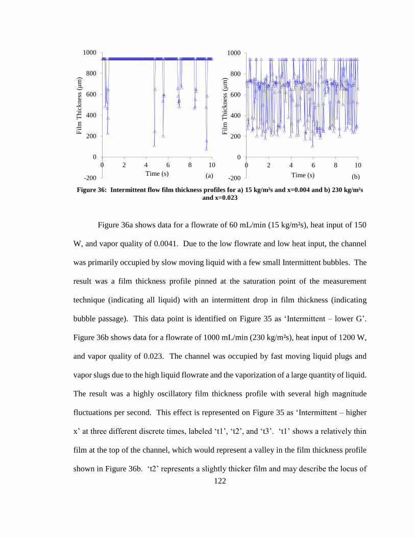
122
Figure 36: Intermittent flow film thickness profiles for a) 15 kg/m²s and x=0.004 and b) 230 kg/m²s
and x=0.023
Figure 36a shows data for a flowrate of 60 mL/min (15 kg/m²s), heat input of 150
W, and vapor quality of 0.0041. Due to the low flowrate and low heat input, the channel
was primarily occupied by slow moving liquid with a few small Intermittent bubbles. The
result was a film thickness profile pinned at the saturation point of the measurement
technique (indicating all liquid) with an intermittent drop in film thickness (indicating
bubble passage). This data point is identified on Figure 35 as ‘Intermittent – lower G’.
Figure 36b shows data for a flowrate of 1000 mL/min (230 kg/m²s), heat input of 1200 W,
and vapor quality of 0.023. The channel was occupied by fast moving liquid plugs and
vapor slugs due to the high liquid flowrate and the vaporization of a large quantity of liquid.
The result was a highly oscillatory film thickness profile with several high magnitude
fluctuations per second. This effect is represented on Figure 35 as ‘Intermittent – higher
x’ at three different discrete times, labeled ‘t1’, ‘t2’, and ‘t3’. ‘t1’ shows a relatively thin
film at the top of the channel, which would represent a valley in the film thickness profile
shown in Figure 36b. ‘t2’ represents a slightly thicker film and may describe the locus of
-200
0
200
400
600
800
1000
0 2 4 6 8 10
Fil
m T
hic
knes
s (μ
m)
Time (s)-200
0
200
400
600
800
1000
0 2 4 6 8 10
Fil
m T
hic
knes
s (μ
m)
Time (s)(a) (b)

123
data points that fall close to 700 μm on Figure 36b. Finally, the TIR sensor reached the
saturation point of the measurement technique at ‘t3’. Both of the scenarios shown in
Figure 36 are experimentally defined as Intermittent flow (both here and for the duration
of the Dissertation), but were differentiated here for academic purposes.
Another subtle difference between the ideal cases and actual experimental cases is
the presence of unstable Slug-Annular flow as an intermediate sub-regime between the
Slug flow and Annular flow regimes for moderate flowrates, 250 and 500 mL/min (60-125
kg/m²s), and vapor qualities exceeding 0.01. Other researchers have observed this
phenomenon and referred to this regime as Aerated Slug [141] [158], Slug/Semi-Annular
[159], and churn flow.
Two examples of the unstable film thickness profile characteristic of Slug-Annular
flow are shown in Figure 37. Slug-Annular flow had characteristics of both Annular and
Intermittent flow. For both cases, Slug-Annular flow was marked by an unstable film,
similar to the ideal Annular flow case in Figure 34, with the passage of an occasional liquid
plug, similar to the Intermittent flow cases in Figure 34 and Figure 36. For a flowrate of
250 mL/min (60 kg/m²s) and vapor quality of 0.014, the passing liquid plugs were thick
enough to saturate the film thickness measurement technique. Figure 35 shows Slug-
Annular high speed photographs for this operating condition, labeled as ‘Slug-Annular –
lower x’ at three different time steps. As the time progresses from ‘t1’ to ‘t3’, it can be
seen that the film thickness progresses from relatively thin to thick, resulting in occasional
saturation of the measurement technique and the film thickness profile shown in Figure
37a. However, as the vapor quality increased from 0.014 to 0.066 in Figure 37b, the liquid
plugs reduced in thickness and did not saturate the technique. In other words, as vapor

124
quality increased the film thickness profile appeared to approach a more-Annular (and less
Intermittent) operating condition. This is shown in Figure 35, labeled as ‘Slug-Annular –
higher x’ at three different time steps, where the film fluctuates from relatively thin to
relatively thick without completely saturating the technique.
Figure 37: Film thickness profile for intermediate Slug-Annular flow with a) 60 kg/m²s and x=0.014
and b) 60 kg/m²s and x=0.066
For the HFE-7100 results in Chapter 8, the flow regime is defined as Annular flow
if a thin film is present but the technique is not saturated (Figure 37b) and Intermittent flow
if the passing liquid plug saturates the technique (Figure 37a). However, one could be
inclined to believe that the profile shown in Figure 37b is representative of Intermittent
flow, as well. Therefore, it’s necessary to acknowledge that this method is not fully-
objective. In order to classify the film thickness profiles into useful flow regime categories,
objective qualifiers must be chosen or set. Such is the case with differentiating between
Intermittent and Annular flow in Figure 37a and Figure 37b, above. However, when these
classifications are well argued and consistently applied, this method provides a much less
subjective, and much more repeatable method for determining flow regime.
-200
0
200
400
600
800
1000
0 2 4 6 8 10
Fil
m T
hic
knes
s (μ
m)
Time (s)-200
0
200
400
600
800
1000
0 2 4 6 8 10
Fil
m T
hic
knes
s (μ
m)
Time (s)(a) (b)

125
6.4.5 TIR Validation with Existing Flow Regime Maps
Horizontal two-phase flow regime data was collected, using the TIR method at the
top of an 8.84mm ID transparent tube, across the parametric space described in Section
6.3.2. Then, the data was converted to a usable form and plotted on the Taitel-Dukler [46],
Ullmann-Brauner [141], and Wojtan et al. [30] flow regime maps using Equations (50)-
(53).
Three dominant experimental flow regimes were observed; Stratified;
Intermittent/Slug; and Slug-Annular as an intermediate flow regime between Slug and
Annular flow. It is to be noted that unlike the eight unique flow regimes defined by the
Wojtan et al. [30] map, most two-phase researchers [55] have limited their classification to
the Bubbly, Intermittent, Stratified, and Annular flow. In the interest of uniformity and
consistency, and to avoid confusion that may derive from the diversity of names used by
authors for some of the observed sub-regimes, the classifications of flow regime beyond
this chapter will follow the classification proposed by Rahim et al. [55], combining Slug,
Plug, and Intermittent data points into Intermittent flow, combining Slugging-Annular
flow, Wavy-Annular flow, and Semi-Annular data into Annular flow, and defining
Stratified-Wavy flow as a sub-regime of Stratified flow, leading to the presence of just 4
primary regimes: Stratified, Bubbly, Intermittent, and Annular. For the remainder of this
chapter, however, the sub-regime of Slug-Annular flow is differentiated to further
demonstrate the capabilities and subtleties of the optical technique.
Figure 38 shows the experimental data plotted on the three respective flow regime
maps. The circle data points are Stratified observations, the triangular data points are the
Intermittent/Slug observations, and the square data points are the Slug-Annular

126
observations. It should be noted that the transition boundaries on these flow regime maps
are typically ±25%, so data points on or near the border may fall within this error band.
The Taitel-Dukler [46] flow regimes are marked in coordinates of superficial liquid
velocity and superficial gas velocity with the transition locus for Stratified, Intermittent,
Annular, and Bubbly flow marked by solid black lines. The Ullmann-Brauner [141] map,
displayed in the same coordinates as Taitel-Dukler [46], plotted Stratified flow, Slug flow,
Aerated Slug flow, Annular flow, Bubbly flow, and Dispersed Bubbly flow with solid lines
separating the flow regimes. The Wojtan et al. [30] flow regime map plotted Stratified
flow, Stratified-Wavy flow, Slug and Stratified-Wavy flow, Slug flow, Intermittent flow,
and Annular flow in coordinates mass flux and vapor quality with solid lines separating the
flow regimes.
Data points at higher superficial liquid velocity or mass flux correspond to higher
flowrate (1000, 500, 250, 125, or 62 mL/min). Superficial liquid velocity decreased
slightly for a fixed flowrate and increasing vapor quality according to Equation (52).
However, superficial vapor velocity increased significantly as vapor quality increased, as
shown by Equation (53). Therefore, tracking horizontally from left to right on these flow
regime maps provides flow regime data for a fixed flowrate with increasing vapor quality.
For a flowrate of 1000 mL/min (225 kg/m²s), the vapor quality ranged from 0.0001
to 0.0232 and the observed fluctuations in film thickness always corresponded to
Intermittent/Slug flow. The data point labeled ‘Ideal Intermittent’ on Figure 38 represents
the ideal Intermittent film thickness profile shown in Figure 34 and visually in Figure 35.
The data point labeled ‘Intermittent – higher x’ represents the highly oscillatory
Intermittent film thickness profile shown in Figure 36b and visually in Figure 35.

127
Figure 38: Two-Phase flow regime data plotted on a) Taitel-Dukler [46] map, b) Ullmann-Brauner
[141] map, and c) Wojtan et al. [30] map
0.001
0.01
0.1
1
10
0.01 0.1 1 10 100
Sup
erfi
cial
Liq
uid
Vel
oci
ty (
m/s
)
Superficial Gas Velocity (m/s)
Bubbly
Annular
Intermittent
Stratified
0.001
0.01
0.1
1
10
0.01 0.1 1 10 100
Sup
erfi
cial
Liq
uid
Vel
oci
ty (
m/s
)
Superficial Gas Velocity (m/s)
Slug
Aereated
Slug
Dispersed Bubbly
Bubbly
Annular
Stratified
0
50
100
150
200
250
0 0.1 0.2 0.3 0.4
G (
kg/m
²s)
x
Stratified Slug-Annular Intermittent
Slug
Slug and
Stratified
-Wavy
Stratified
Intermittent
Stratified-Wavy
Annular
0
50
100
150
200
250
0 0.1 0.2 0.3 0.4
G (
kg/m
²s)
x
Stratified Slug-Annular Intermittent
Slug
Slug and
Stratified
-Wavy
Stratified
Intermittent
Stratified-Wavy
Annular
(b)
Ideal Intermittent
Intermittent – higher x
Intermittent – lower G
Ideal Stratified
Annular
Slug-Annular - higher x
Slug-Annular - lower x
Ideal Intermittent
Intermittent – higher x
Ideal Stratified
Annular
Slug-Annular - higher x
Slug-Annular - lower x
Intermittent – lower G
Annular
(c)
(a)

128
For a flowrate of 500 mL/min (120 kg/m²s) the vapor quality ranged from 0.0003
to 0.0353. The flow regime started as Intermittent/Slug flow at low vapor quality but
transitioned to Slug-Annular flow at higher vapor quality and superficial gas velocity. The
data point labeled ‘Slug-Annular - lower x’ represents Slug-Annular flow that has
characteristics closely related to Intermittent flow, as shown in Figure 37a and Figure 35.
The data point labeled ‘Slug-Annular – higher x’ represents Slug-Annular flow at higher
vapor quality that more closely resembles Annular flow, as shown in Figure 37b and Figure
35. The flow regime would presumably transition to the data point labeled ‘Annular’, the
Annular flow film thickness profile shown in Figure 34 and Figure 35, if more heat was
added to the system.
With a flowrate of 250 mL/min (60 kg/m²s), the vapor quality ranged from 0.0016
to 0.066 and, similar to the 500 mL/min (120 kg/m²s) case, the flow regime started as
Intermittent/Slug flow at low vapor quality but transitioned to Slug-Annular flow at higher
vapor quality. At a flowrate of 125 mL/min (30 kg/m²s), the vapor quality ranged from
0.0002 to 0.129 and the flow regime transitioned from Intermittent/Slug flow to Stratified
flow at vapor qualities greater than 0.02.
For a flowrate of 60 mL/min (15kg/m²s), the vapor quality ranged from 0.004 to
0.319 and, similar to 125 mL/min, the flow regime was Intermittent/Slug at low vapor
quality and appeared to transition to Stratified flow at qualities greater than 0.3. The data
point labeled ‘Intermittent – lower G’ represents Intermittent/Slug flow at low flowrate and
low vapor quality resulting in a channel primarily occupied by slow moving liquid with a
few Intermittent bubbles as shown in Figure 36a and Figure 35. The data point labeled

129
‘Ideal Stratified’ represents the ideal Stratified film thickness profile shown in Figure 34
and Figure 35.
All three flow regime maps accurately predicted the primary flow regimes shown
in Figure 34 and identified by the labeled data points on Figure 35 and Figure 38. The flow
regime maps also accurately predicted the natural transition from Intermittent/Slug flow to
Annular flow with increasing vapor quality and superficial vapor velocity, as well as other
trends as discussed above. Deviation in predictive accuracy arose when observing the full
parametric space tested for a variety of flow rates and vapor qualities. The predominance
of Slug-Annular flow suggests that the transition from one flow regime to another cannot
necessarily be identified by a discrete point or curve, but rather a range of operating
conditions. Along these same lines, it is to be noted that the observed discrepancy between
predicted and measured flow regimes for data in the literature is commonly within a ±25%
band.
In addition to general trends and ideal cases consistent from one map to the next,
the results agreed reasonably well with the Taitel-Dukler [46] flow regime map. Every
Stratified data point is correctly predicted, every Intermittent/Slug flow data point at 1000
mL/min, over the full range of vapor qualities tested is predicted, and the model appears to
predict the transition towards more-Annular flow for 250 and 500 mL/min. The Taitel-
Dukler [46] flow regime map does not correctly predict the parametric space occupied by
Intermittent flow at relatively low superficial gas velocity (less than 1 m/s). From Figure
38, it incorrectly predicts these Intermittent data points as Stratified flow. However, these
data points exist at low heat dissipation and low vapor quality which are of little importance
in most practical applications.

130
The Ullmann-Brauner [141] model reflects trends indicative of the experimental
data and matches closely with many data points. It predicts the correct vicinity of the
Stratified flow regime and identifies that this flow regime may occupy a smaller parametric
space than previously hypothesized by Taitel-Dukler [46]. Additionally, the Ullmann-
Brauner [141] map identifies the possibility to transition from Intermittent/Slug flow to
Stratified flow at low flowrate and increasing vapor quality. Three additional trends the
Ullmann-Brauner [141] map accurately captures are; presence of Annular flow at higher
superficial gas velocity; dominance of the Aerated Slug regime as an intermediate regime
between Slug and Annular flow; and extension of Intermittent/Slug flow regime to lower
superficial liquid and vapor velocities.
The Wojtan et al. [30] flow regime map accurately predicts all of the Stratified data
points. This map also accurately predicts the dominance of Intermittent/Slug flow at low
vapor quality across a wide range of flowrates. One exception is at very low mass flux and
vapor quality where Intermittent/Slug data points are incorrectly predicted as Stratified
flow. However, these data points exist at low heat dissipation and low vapor quality which
are of little importance in most applications and occupy a very small region of the operating
space. The Wojtan et al. [30] map also predicts the natural progression from Slug-Annular
flow at 500 mL/min (120 kg/m²s) to Annular flow, the data point labeled ‘Slug-Annular –
higher x’, with increasing vapor quality. One discrepancy is the location of the Annular
flow regime with relation to the observed Slug-Annular data points for 250 mL/min (50
kg/m²s). From Figure 37, it was shown that as vapor quality increases from 0.014 to 0.066
the liquid slugs reduce in thickness and do not saturate the measurement technique. In
other words, as vapor quality increases the film thickness profile appears to approach a

131
more-Annular (and less Intermittent) operating condition. However, with a fixed flowrate
of 250 mL/min (50 kg/m²s) the Wojtan et al. [30] map predicts transition to Stratified-
Wavy flow, not Annular flow. A likely explanation for this deviation is that the Wojtan et
al. [30] flow regime map was empirically fit to match common refrigerants, which have
fluid properties vastly different than water (see Table 7). In effect, the empirical constants
allow for better predictive accuracy for operating conditions close to the data set used to
develop the correlations, but do not extrapolate well to different conditions. Conversely,
due to the generality of the Taitel-Dukler [46] and Ullmann-Brauner [141] flow regime
maps, they can often be ‘less accurate’ at times but applicable to a wider range of fluids
and operating conditions. Consequently, the Taitel-Dukler [46] and Ullman-Brauner [141]
maps both predict transition to Annular flow at a fixed flowrate of 250 mL/min and
increasing vapor quality with water as the working fluid.
The three maps above all correctly predicted the primary flow regimes, the natural
transition from Intermittent/Slug flow to Annular flow with increasing vapor quality and
superficial vapor velocity, as well as other trends. No single flow regime map accurately
predicted every data point, however, each individual map did provide specific advantages
and the ability to predict certain flow regimes better than others (with water as the working
fluid). As suggested by Rahim et al. [55], and consistent with trends in the current study,
a combination of these maps might better predict the prevailing flow regimes.
6.5 Summary
An optical, non-intrusive, flow pattern identification method was developed to
validate flow regime maps for two-phase adiabatic water/vapor/nitrogen flow in an 8.84
mm diameter tube. The method consisted of shining a red fiber-optic light source through

132
the top of an optically transparent glass tube, using a CMOS camera to capture light rings
resulting from total internal reflection at the liquid-vapor interface, and extracting a film
thickness profile from the resulting images. It was found that different flow regimes
resulted in unique temporally varying film thickness profiles, which were confirmed using
high speed visualization. Using these profiles, quantitative flow regime identification
measures were developed, including the ability to explain and quantify the more subtle
transitions that exist between dominant flow regimes. This method is applicable to two-
phase flow in transparent tubes and substrates alike, with a variety a working fluids.
The principal flow regimes, Stratified, Intermittent/Slug, and Annular flow were
experimentally observed. Additionally, Slug-Annular flow as an intermediate flow regime
between Intermittent/Slug and Annular flow was observed and quantified. The
phenomenological flow regime maps of Taitel-Dukler [46], Ullmann-Brauner [141], and
Wojtan et al. [30] were found to capture the smooth tube experimental data, with varying
accuracy, validating the use of the TIR technique in predicting flow regime. Please note,
sub-regimes were described here to demonstrate the capabilities of the technique, however,
in Chapter 8 flow regime definitions will be simplified to avoid overcomplicating the data
and analysis.

133
Chapter 7: Single-Phase Data and Discussion
This chapter considers heat transfer rates for horizontal in-tube single-phase flows.
Single-phase tests were performed with the three-different smooth and internally-grooved
tubes described in Table 8, coated with the thin-film heaters described in Section 5.2, and
operating with HFE-7100 as the working fluid. Theoretical predictions were compared to
the experimental results to determine the accuracy and reliability of the test setup and to
assess the accuracy of single-phase, smooth and internally-grooved tube, heat transfer
models in the literature.
7.1 Single-Phase Energy Balance
As described in Chapter 5, a single-phase energy balance was first performed to
ensure that the majority of the heat electrically applied to the system was entering the fluid
and to make sure the thermofluid delivery and measurement system was calibrated and
working properly. This step was an essential first-step for validating the test setup; without
this analysis, the local and exit vapor qualities as well as the experimental heat transfer
coefficients during two-phase testing cannot be trusted. For these tests, the fluid inlet
temperature was held around 15ºC and the tube outside wall temperature was not allowed
to exceed 61ºC, the boiling temperature of HFE-7100 at atmospheric pressure. This
reduced the likelihood of pseudo-boiling (air coming out of the solution) and the
occurrence of sub-cooled flow boiling, which could affect the heat transfer coefficient. The
input energy was the electrical power applied to the system. The output energy was
calculated based on the fluid temperature rise, ∆T, mass flowrate, m, and specific heat, Cp,
based on the equation below:

134
Qout = mCp∆T (56)
Figure 39 shows the single-phase energy balance ratio for the 2.8mm, 4.54mm, and
8.84mm smooth tubes with a heat flux of 18 kW/m², mass fluxes ranging from 150 to 1100
kg/m²s, and HFE-7100 as the working fluid. The ratio of heat out to heat in, as measured
through the temperature rise in the fluid, was generally less than 1 but always greater than
0.95. This reveals that there is a minor source of heat loss and measurement uncertainty in
the system. However, the results are always within ±5% of the expected value, which is
considered acceptable for the current study.
Figure 39: Single-phase liquid energy balance ratio for HFE-7100 in different tube diameters
7.2 Single-Phase Heat Transfer Measurements and Comparison to Smooth Tube
Correlations
Measured heat transfer coefficients for the 2.8mm, 4.54mm, and 8.84mm smooth
tubes with a heat flux of 18 kW/m², mass fluxes ranging from 150 to 1100 kg/m²s, and
HFE-7100 as the working fluid were compared to the two correlations of Dittus-Boelter
(‘common’ and ‘original’ form), Colburn, and Gnielinski; all four correlations were taken
from the Incropera et al. Fundamentals of Heat and Mass Transfer Handbook [25]. Since
0.9
0.95
1
1.05
1.1
0 200 400 600 800 1000 1200
Qo
ut/
Qin
G (kg/m²s)0.9
0.95
1
1.05
1.1
0 200 400 600 800 1000 1200
8.84 mm 4.54 mm 2.8 mm

135
turbulent flow is convoluted, emphasis has been placed on empirical correlations. The
‘common’ Dittus-Boelter correlation for heating takes the form:
NuD = 0.023Re0.8Pr0.4 (57)
where Re is the Reynolds number and Pr is the Prandtl number. The ‘original’ Dittus-
Boelter equation for heating is of the form:
NuD = 0.0243Re0.8Pr0.4 (58)
The Colburn equation is:
NuD = 0.023Re0.8Pr0.333 (59)
Finally, the Gnielinski correlation, which is valid over a large Reynolds number range
(3000<Re<5x10⁶), takes the form:
NuD =(
f8
) (Re − 1000)Pr
1 + 12.7 (f8
)0.5
(Pr0.667 − 1)
(60)
where f is friction factor, which can be obtained from a Moody diagram or calculated
directly for smooth tubes as:
f = (0.790 ln Re − 1.64)−2 (61)
Figure 40 shows the experimental single-phase heat transfer coefficient vs mass
flux results, compared to the predictions. The properties used while evaluating these
correlations were the average values between the inlet and outlet of the test section. The
results show that the heat transfer coefficient increases with increasing flowrate, for all
three tube diameters, to the power of approximately 0.8; the reader is directed to the
correlations shown in Equation (57)-(59) where the Reynolds number is raised to the power
of 0.8. For a fixed flowrate, heat transfer coefficients slightly increased as the tube
diameter decreased. These trends are predicted well by the correlations.

136
Figure 40: Experimental and predicted single-phase heat transfer coefficient vs mass flux for a) 8.84
mm smooth tube, b) 4.54 mm smooth tube, and c) 2.8 mm smooth tube
0
100
200
300
400
500
600
0 100 200 300 400 500
Hea
t T
ransf
er C
oef
fici
ent
(W/m
²K)
G (kg/m²s)
0
200
400
600
800
1000
1200
1400
0 200 400 600 800 1000 1200
Hea
t T
ransf
er C
oef
fici
ent
(W/m
²K)
G (kg/m²s)
0
200
400
600
800
1000
1200
1400
1600
0 200 400 600 800 1000
Hea
t T
ransf
er C
oef
fici
ent
(W/m
²K)
G (kg/m²s)
0100200300400500600
0 100 200 300 400 500
G (kg/m²s)
experimental Dittus-Boelter common Dittus-Boelter original Colburn Gnielinski
a)
c)
b)
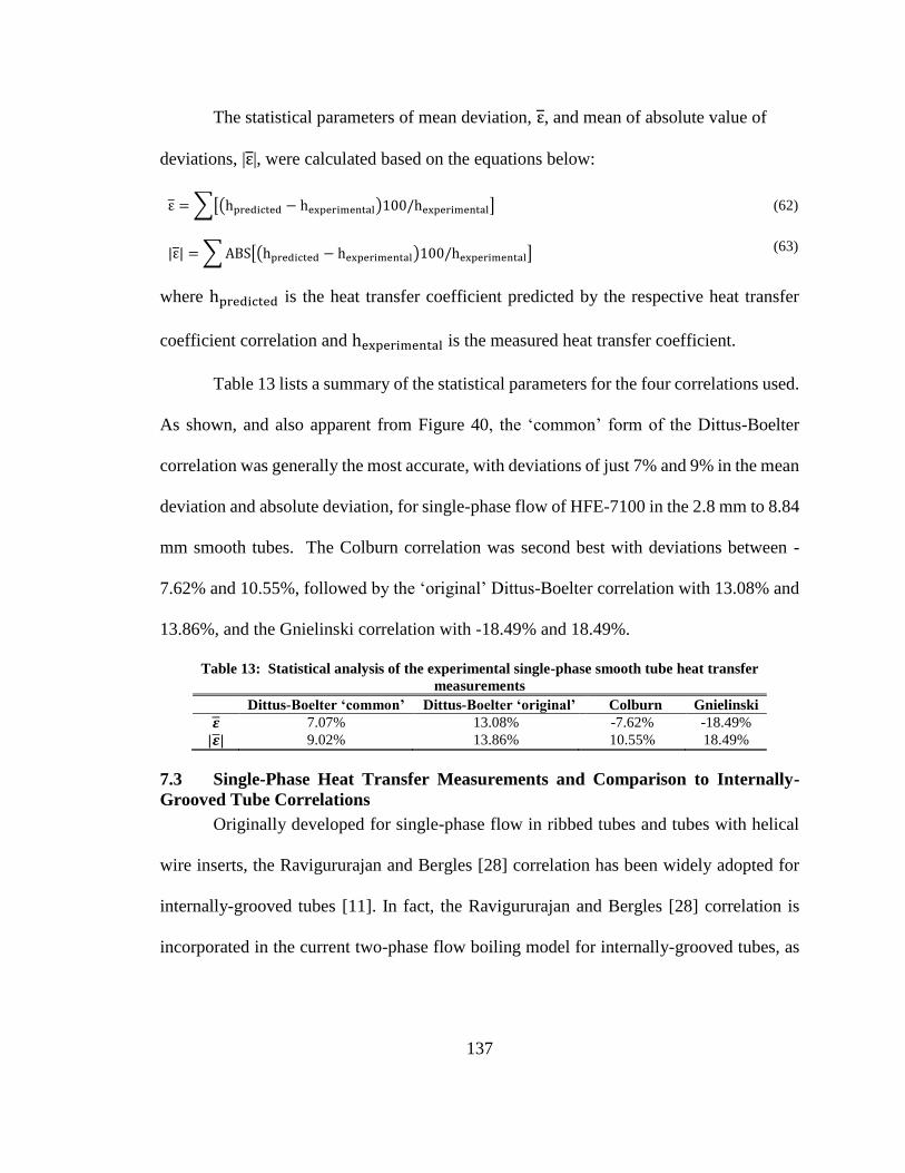
137
The statistical parameters of mean deviation, ε, and mean of absolute value of
deviations, |ε|, were calculated based on the equations below:
ε = ∑[(hpredicted − hexperimental)100/hexperimental] (62)
|ε| = ∑ ABS[(hpredicted − hexperimental)100/hexperimental] (63)
where hpredicted is the heat transfer coefficient predicted by the respective heat transfer
coefficient correlation and hexperimental is the measured heat transfer coefficient.
Table 13 lists a summary of the statistical parameters for the four correlations used.
As shown, and also apparent from Figure 40, the ‘common’ form of the Dittus-Boelter
correlation was generally the most accurate, with deviations of just 7% and 9% in the mean
deviation and absolute deviation, for single-phase flow of HFE-7100 in the 2.8 mm to 8.84
mm smooth tubes. The Colburn correlation was second best with deviations between -
7.62% and 10.55%, followed by the ‘original’ Dittus-Boelter correlation with 13.08% and
13.86%, and the Gnielinski correlation with -18.49% and 18.49%.
Table 13: Statistical analysis of the experimental single-phase smooth tube heat transfer
measurements
Dittus-Boelter ‘common’ Dittus-Boelter ‘original’ Colburn Gnielinski
𝜺 7.07% 13.08% -7.62% -18.49%
|𝜺| 9.02% 13.86% 10.55% 18.49%
7.3 Single-Phase Heat Transfer Measurements and Comparison to Internally-
Grooved Tube Correlations
Originally developed for single-phase flow in ribbed tubes and tubes with helical
wire inserts, the Ravigururajan and Bergles [28] correlation has been widely adopted for
internally-grooved tubes [11]. In fact, the Ravigururajan and Bergles [28] correlation is
incorporated in the current two-phase flow boiling model for internally-grooved tubes, as

138
described in Chapter 4, Equation (36). The final, normalized, heat transfer coefficient for
internally-grooved tubes is given by:
Nurb/Nus = Erb = 1 + [2.64Re0.36PrL−0.024 (
ef
df)
0.212
(pf
df)
−0.21
(αf
90°)
0.29
]7
1/7
(64)
where ef is the groove height, df is the nominal inside diameter at the fin base, pf is the
axial pitch from groove to groove, and αf is the helix angle of the grooves. As shown in
Equation (64) and discussed in Chapter 4, the single-phase turbulent correlation developed
by Ravigururajan and Bergles [28] was described as an ‘enhancement’ over a comparable
smooth tube. For the current analysis, the reference smooth-tube heat transfer correlations
will be the two correlations of Dittus-Boelter (‘common’ and ‘original’ form), Colburn,
and Gnielinski; all four correlations were taken from the Incropera et al. Fundamentals of
Heat and Mass Transfer Handbook [25] and are described formulaically above. The
‘common’ Dittus-Boelter correlation adjusted for predicting heat transfer coefficient in
internally-grooved tubes becomes:
NuD = Erb0.023Re0.8Pr0.4 (65)
The ‘original’ Dittus-Boelter equation for heating takes the form:
NuD = Erb0.0243Re0.8Pr0.4 (66)
The Colburn equation is now:
NuD = Erb0.023Re0.8Pr0.333 (67)
Finally, the Gnielinski correlation becomes:
NuD =Erb (
f8
) (Re − 1000)Pr
1 + 12.7 (f8
)0.5
(Pr0.667 − 1)
(68)
where f is the smooth-tube friction factor, which can be calculated directly:

139
f = (0.790 ln Re − 1.64)−2 (69)
Figure 41 shows the measured and predicted (based on Equations (65)-(68) above)
heat transfer coefficients for the 2.62mm, 4.54mm, and 8.84mm internally-grooved tubes
with a heat flux of 18 kW/m², mass fluxes ranging from 150 to 1100 kg/m²s, and HFE-
7100 as the working fluid. The properties used while evaluating these correlations were
the average values between the inlet and outlet of the test section. The results show that
the heat transfer coefficient increases with increasing flowrate, for all three tube diameters.
For a fixed flowrate, heat transfer coefficients slightly increased as the tube diameter
decreased.
Table 13 lists a summary of the statistical parameters for the four correlations used.
As shown, the ‘common’ form of the Dittus-Boelter correlation (adjusted with the
Ravigururajan and Bergles [28] enhancement factor) was generally the most accurate for
the range of internally-grooved tube diameters and mass fluxes tested, with mean and
absolute deviations of only 4.46% and 11.08%. The Colburn correlation was second best
with deviations between -9.87% and 10.56%, followed by the ‘original’ Dittus-Boelter
correlation with 10.33% and 13.91%, and the Gnielinski correlation with -23.38% and
26.26%. These predictive trends are consistent with those reported for the smooth tubes.
Table 14: Statistical analysis of the experimental single-phase internally-grooved tube heat transfer
measurements
Dittus-Boelter ‘common’ Dittus-Boelter ‘original’ Colburn Gnielinski
𝜺 4.46% 10.33% -9.87% -23.38%
|𝜺| 11.08% 13.91% 10.56% 26.26%

140
Figure 41: Experimental and predicted single-phase heat transfer coefficient vs mass flux for a) 8.84
mm internally-grooved tube, b) 4.54 mm internally-grooved tube, and c) 2.62 mm internally-grooved
tube
0
200
400
600
800
1000
0 100 200 300 400 500
Hea
t T
ransf
er C
oef
fici
ent
(W/m
²K)
G (kg/m²s)
0
400
800
1200
1600
2000
2400
0 200 400 600 800 1000 1200
Hea
t T
ransf
er C
oef
fici
ent
(W/m
²K)
G (kg/m²s)
0
300
600
900
1200
1500
1800
0 200 400 600 800 1000 1200
Hea
t T
ransf
er C
oef
fici
ent
(W/m
²K)
G (kg/m²s)
0100200300400500600
0 100 200 300 400 500
G (kg/m²s)
experimental Dittus-Boelter common Dittus-Boelter original Colburn Gnielinski
a)
c)
b)

141
The above single-phase energy balance and single-phase heat transfer statistical
analysis indicates that the test setup is functioning properly and the experimental method
is robust and can provide reliable measurements. This analysis also justifies the use of the
Ravigururajan and Bergles [28] enhancement factor, Erb, for predicting turbulence effects
resulting from the groove structures in the two-phase internally-grooved tube correlation
developed in Chapter 4.

142
Chapter 8: Two-Phase Data and Discussion
This chapter outlines the experimental validation of the physics-based heat transfer
coefficient model described Chapter 4 that recognizes the role played by two-phase flow
structures in enhancing thermal transport within internally-grooved tubes. Flow regime
data, obtained with dynamic total-internal-reflection measurements described in Chapter
6, and heat transfer coefficient data, obtained with infrared thermography and the test setup
described in Chapter 5, are presented and analyzed for two-phase HFE-7100 flow in
horizontal, 2.62-8.84 mm diameter, smooth and internally-grooved tubes, with mass fluxes
from 25-300 kg/m²s, heat fluxes from 4-56 kW/m², and exit vapor qualities approaching 1.
First, the flow regime results are compared to the Wojtan et al. [30] smooth tube
map and the Sharar et al. [29] internally-grooved tube map. Next, the smooth tube and
internally-grooved tubes heat transfer results will be compared at varying mass fluxes and
heat fluxes to illustrate the validity of the current regime-based approach to explaining
enhancement in internally-grooved tubes. This data is then used to statistically validate the
new flow regime based heat transfer coefficient correlation, as well as correlations from
the literature. Finally, the new heat transfer model will be compared to independent data
in the literature and the chapter results will be summarized.
An extensive heat transfer coefficient and flow regime database of over 6,500
combined data points for the adiabatic and diabatic smooth and internally-grooved tubes,
respectively, was acquired. For the sake of brevity, only select data and figures will be
used to explain the points above. Please refer to Appendix C - Appendix E for all of the
heat transfer data collected and Appendix F for a more comprehensive statistical analysis

143
of the correlations for smooth and internally-grooved tubes – only summaries and selected
results are given herein.
As reported in the error analysis in Chapter 5, the reported heat transfer coefficients
in the internally-grooved tubes are average augmented values accounting for the increased
area enhancement. Therefore, uncertainty stemming from ambiguity in the reported area
enhancement is not propagated in the heat transfer error measurement. However, when
normalizing the results to account for area enhancement in summary charts, it should be
expected that small ~1-5% error (based on a conversation with Wieland and the
understanding that this is a carefully controlled industrial process) is introduced due to
slight manufacturing deviations.
8.1 8.84mm Smooth and Internally-Grooved Tubes
8.1.1 Influence of Mass Flux and Flow Regime
Figure 42 shows the adiabatic results of the flow visualization/quantification,
plotted in coordinates of mass flux and vapor quality and superimposed on the smooth tube
and internally-grooved tube flow regime maps; Figure 42a is the smooth tube experimental
results on the Wojtan et al. [30] map, Figure 42b is the internally-grooved tube results
plotted on the Wojtan et al. map [30], and Figure 42c is the internally-grooved tube data
plotted on the current Sharar et al. [29] map. Stratified data points are represented by red
circles, Intermittent data points are blue triangles, and Annular data points are shown by
green squares. Please note, for figure clarity, the diabatic flow visualization results are not
shown but the adiabatic data points shown on Figure 42 are representative of the flow
trends observed.

144
Figure 42: 8.84mm smooth tube data plotted on a) the Wojtan et al. [30] map and 8.84mm
internally-grooved tube data plotted on b) the Wojtan et al. [30] map and c) the Sharar et al. [29]
map with HFE-7100 at 61°C, G=50 kg/m²s, and q”=9 kW/m²
0
100
200
300
400
500
0.0 0.1 0.2 0.3 0.4 0.5 0.6 0.7 0.8 0.9 1.0
G (
kg/m
²s)
x
G stratified G stratified-wavy
0
100
200
300
400
500
0.0 0.1 0.2 0.3 0.4 0.5 0.6 0.7 0.8 0.9 1.0
G (
kg/m
²s)
x
G stratified G stratified-wavy
0
100
200
300
400
500
0.0 0.1 0.2 0.3 0.4 0.5 0.6 0.7 0.8 0.9 1.0
G (
kg/m
²s)
x
Stratified Intermittent Annular
a)
b)
c)
Intermittent
Annular
Slug
Slug and
Stratified -
Wavy
Stratified Stratified-Wavy
Dryout
Mist
Intermittent
Annular
Slug and
Stratified -
Wavy
Stratified Stratified-Wavy
Dryout
Mist
Intermittent
Annular
Slug and
Stratified -
Wavy
Stratified Stratified-Wavy
Dryout
Mist
Slug
Slug

145
The transitions of flow pattern observed were Stratified, Intermittent, and Annular
in the direction of increasing G and x. It’s apparent from Figure 42 that the transition to
Annular flow in the internally-grooved tube is seen to occur at lower mass flux and vapor
quality compared to the smooth tube. For example, at a mass flux of G=75 kg/m²s and
vapor quality greater than x=0.4, Annular flow was encountered in the internally-grooved
tube while the smooth tube was operating in Stratified flow. In fact, Annular flow did not
occur in the smooth tube for mass fluxes below G=125 kg/m²s while the internally-grooved
tube was found to sustain Annular flow at mass fluxes as low as G=50 kg/m²s.
In addition to early Stratified-to-Annular transition, the internally-grooved tube
provided early transition from Intermittent to Annular flow at higher mass fluxes. As an
example, at a mass flux of G=200 kg/m²s and vapor quality greater than x=0.1 the
internally-grooved tube is operating in Annular flow. This transition does not occur in the
smooth tube until a vapor quality of approximately 0.3.
It’s also interesting to note that at sufficiently low mass fluxes, G<25 kg/m²s, both
the smooth and internally-grooved tubes are operating in Stratified flow. Similarly, at
high mass fluxes, G>125 kg/m²s, and high vapor qualities, x=0.3, both the smooth tube and
the internally-grooved tube are operating in Annular flow. As shown in Figure 42a, the
Wojtan et al. [30] flow regime map captures these smooth tube trends well, correctly
predicting 178/197 flow regime data points (90.3%). However, as shown in Figure 42b
the Wojtan et al. [30] map does a poor job predicting flow regime in the internally-grooved
tube, correctly predicting only 122/186 data points (65.6%). The Sharar et al. [29]
modified flow regime map shown in Figure 42c correctly predicted 164/186 (87.7%) of the
flow regime data in the internally-grooved tube, representing a 22% improvement in

146
predictive accuracy of the traditional Wojtan et al. [30] model. It’s worth mentioning that
the new model does mis-predict a number of Annular data points at low mass flux and high
vapor quality; this is clear in Figure 42c at vapor qualities greater than 0.4 and a mass flux
of 50 kg/m²s.
Figure 43 shows a comparison of experimental heat transfer coefficients for the
smooth and internally-grooved tubes with HFE-7100 at a heat flux of 9 kW/m² for three
mass fluxes; Figure 43a is a mass flux of 25 kg/m²s, Figure 43b is a mass flux of 75 kg/m²s,
and Figure 43c is a mass flux of 200 kg/m²s. The experimental smooth tube data points
are shown as red squares and the internally-grooved tube data points are green circles. ‘IG
1’ and ‘smooth 1’ were the first tests run and ‘IG 2’ and ‘smooth 2’ were the second tests
run; these do not represent different tubes, just a second set of experiments for validation.
The smooth tube heat transfer coefficient correlation as described by Wojtan et al. [31] and
the internally-grooved tube heat transfer coefficient correlation, described in the current
study, are plotted as solid red and dashed green lines, respectively.
As can be seen in Figure 43a, the smooth and internally-grooved tube heat transfer
coefficients remain low over the full range of vapor qualities tested for a mass flux of 25
kg/m²s. This is a result of the prevalence of Stratified flow in both the smooth and
internally-groove tube, as shown in Figure 43 and discussed above. At a mass flux of 25
kg/m²s the smooth and internally-grooved tubes have θdry values between 0 to 2π. Since
early flow regime transition has not occurred in the internally-grooved tube, the full
enhancement effect, combining area enhancement with favorable regime transition, has not
been observed. In this case, the internally-grooved tube enhancement ratio, defined as the

147
grooved tube heat transfer coefficient divided by the smooth tube coefficient, is close to
the area enhancement, 1.5.
As shown in Figure 43b, the smooth tube heat transfer coefficient for a mass flux
75 kg/m²s is similar to Figure 43a and remains low over the full range of vapor qualities
tested. Again, this is due to the prevalence of Stratified flow and a large dry perimeter
(θdry≠0). This is evident from Figure 42a at a mass flux of 75 kg/m²s where the smooth
tube is consistently operating in Stratified flow. However, the trend for the internally-
grooved tube is much different from Figure 42a as a result of early transition to Annular
flow and a fully wetted perimeter (θdry=0). As can be seen in Figure 42b/c, at 75 kg/m²s
and vapor qualities greater than x=0.4, Annular flow was encountered in the internally-
grooved. The result is a progressively higher heat transfer coefficient as vapor quality
increases, Annular flow develops in the tube, and the Annular film thins. Eventually,
dryout occurs at vapor qualities close to 1 and the heat transfer coefficient significantly
reduces to a value close to the smooth tube values. In this case, the internally-grooved tube
enhancement ratio reaches a maximum value of close to 6.5 at high vapor quality, where
thin film Annular flow prevails in the internally-grooved tube and Stratified flow persists
in the smooth tube. The practical benefit of operating at this low mass flux where the
enhancement is shown to be 6.5x is the reduction in pumping power associated with this
operating condition.

148
Figure 43: Comparison of heat transfer coefficient vs vapor quality for a mass flux of a) 25 kg/m²s,
b) 75 kg/m²s, and c) 200 kg/m²s with HFE-7100 at 61°C and q”=9 kW/m² in the 8.84mm tubes
0
2000
4000
6000
8000
10000
12000
14000
0.0 0.1 0.2 0.3 0.4 0.5 0.6 0.7 0.8 0.9 1.0
Hea
t T
ransf
er C
oef
fici
ent
(W/m
²K)
x
0
2000
4000
6000
8000
10000
12000
14000
0.0 0.1 0.2 0.3 0.4 0.5 0.6 0.7 0.8 0.9 1.0
Hea
t T
ransf
er C
oef
fici
ent
(W/m
²K)
x
0
2000
4000
6000
8000
10000
12000
14000
0.0 0.1 0.2 0.3 0.4 0.5 0.6 0.7 0.8 0.9 1.0
Hea
t T
ransf
er C
oef
fici
ent
(W/m
²K)
x0
100020003000400050006000700080009000
10000110001200013000140001500016000170001800019000
0.0 0.1 0.2 0.3 0.4 0.5 0.6 0.7 0.8 0.9 1.0
Current Wojtan IG 1 IG 2 smooth 1 smooth 2
G = 200 kg/m²s, 9 kW/m²
G = 75 kg/m²s, 9 kW/m²
G = 25 kg/m²s, 9 kW/m²
a)
b)
c)
Modified

149
The trends shown in Figure 43c for a mass flux of 200 kg/m²s are, again, different
from those observed at 25 and 75 kg/m²s. For both the smooth tube and the internally-
grooved tube, the heat transfer coefficients increase monotonically as vapor quality
increases. As shown in Figure 42, this is due to the predominance of Annular flow (θdry=0)
in both the smooth and internally-grooved tube and a thinning Annular film as vapor
quality increases. Similar to the case for 25 kg/m²s, the enhancement factor approaches
the area enhancement at a mass flux of 200 kg/m²s because both tubes are operating in the
same flow regime.
It’s interesting to note that the measured heat transfer coefficient for different runs
of the smooth tube agreed very well for all conditions shown in Figure 43, where it was
operating deep in Stratified or Intermittent/Annular flow. The same is true for 25 kg/m²s
and 200 kg/m²s in the internally-grooved tube where the tube is operating in Stratified or
Intermittent/Annular flow. However, there is more variability between ‘IG 1’ and ‘IG 2’
at a mass flux of 75 kg/m²s near the Stratified-Wavy to Annular transition boundary. More
detail on this point is given in 8.6.2 below.
8.1.2 Influence of Heat Flux
Heat flux has an impact on the contribution of nucleate boiling to thermal transport
from the wetted wall and on dry-out inception and completion. A higher heat flux results
in a higher wall temperature, thus causing faster and more aggressive bubble nucleation,
growth, and departure. Therefore, higher heat flux generally enhances two-phase heat
transfer coefficients. Alternatively, higher heat flux is also observed to yield earlier dryout
at lower vapor quality compared to lower heat fluxes and, consequently, a degraded heat
transfer coefficient. Figure 44 shows heat transfer coefficient vs vapor quality for the

150
8.84mm smooth and internally-grooved tubes for a mass flux of 200kg/m²s and six
different heat fluxes; Figure 44a is a heat flux of 4 kW/m², Figure 44b is a heat flux of 9
kW/m², Figure 44c is a heat flux of 18 kW/m², Figure 44d is a heat flux of 28 kW/m²,
Figure 44e is a heat flux of 40 kW/m², and Figure 44f is a heat flux of 56 kW/m². Please
refer to Appendix C for additional data.
The smooth tube and internally-grooved tube correlations both predict higher heat
transfer coefficients at low vapor quality as the heat flux increases. For example, at a vapor
quality of 0.1 the smooth tube correlation predicts an improvement from 1467 W/m²K to
2386 W/m²K when moving from a heat flux of 4 kW/m² to 56 kW/m² due to nucleate
boiling enhancement. The internally-grooved tube correlation predicts a similar trend and
increases from approximately 3820 W/m²K to 5068 W/m²K with heat fluxes of 4 kW/m²
to 56 kW/m², respectively. However, this enhancement diminishes at higher vapor quality
where nucleate boiling is suppressed and convective vaporization dominates. This is clear
from Figure 44a and Figure 44f where the heat transfer coefficient is approximately 7500
W/m²K for both 4 kW/m² and 56 kW/m² in the internally-grooved tube. Another
interesting effect is a reduction in the vapor quality at which dryout occurs with increasing
heat flux. The vapor quality where dryout occurs changes from 0.91 to 0.63 for the smooth
and internally-grooved tube correlations when moving from 4 kW/m² to 56 kW/m².

151
Figure 44: Comparison of heat transfer coefficient vs vapor quality for the 8.84mm tubes with HFE-
7100 at 61°C and a mass flux of 200 kg/m²s for heat fluxes of a) 4 kW/m², b) 9 kW/m², c) 18 kW/m²,
d) 28 kW/m², e) 40 kW/m², and f) 56 kW/m²
0
2000
4000
6000
8000
10000
12000
14000
0.0 0.1 0.2 0.3 0.4 0.5 0.6 0.7 0.8 0.9 1.0
Hea
t T
ransf
er C
oef
fici
ent
(W/m
²K)
x
0
2000
4000
6000
8000
10000
12000
14000
0.0 0.1 0.2 0.3 0.4 0.5 0.6 0.7 0.8 0.9 1.0
Hea
t T
ransf
er C
oef
fici
ent
(W/m
²K)
x
0
2000
4000
6000
8000
10000
12000
14000
0.0 0.1 0.2 0.3 0.4 0.5 0.6 0.7 0.8 0.9 1.0
Hea
t T
ransf
er C
oef
fici
ent
(W/m
²K)
x
0
2000
4000
6000
8000
10000
12000
14000
0.0 0.1 0.2 0.3 0.4 0.5 0.6 0.7 0.8 0.9 1.0
Hea
t T
ransf
er C
oef
fici
ent
(W/m
²K)
x
0
2000
4000
6000
8000
10000
12000
14000
0.0 0.1 0.2 0.3 0.4 0.5 0.6 0.7 0.8 0.9 1.0
Hea
t T
ransf
er C
oef
fici
ent
(W/m
²K)
x
0
2000
4000
6000
8000
10000
12000
14000
0.0 0.1 0.2 0.3 0.4 0.5 0.6 0.7 0.8 0.9 1.0
Hea
t T
ransf
er C
oef
fici
ent
(W/m
²K)
x0
100020003000400050006000700080009000
10000110001200013000140001500016000170001800019000
0.0 0.1 0.2 0.3 0.4 0.5 0.6 0.7 0.8 0.9 1.0
Current Wojtan IG 1 IG 2 smooth 1 smooth 2
4 kW/m² 9 kW/m²
18 kW/m² 28 kW/m²
40 kW/m² 56 kW/m²
a)
c)
e)
b)
d)
f)
f
x=0.82
d
x=0.801
Modified

152
The correlations were found to accurately predict data with heat fluxes at and below
28 kW/m² but were less accurate for the heat transfer data for higher heat flux values of 40
kW/m² and 56 kW/m². The mean deviation, 𝜀, and mean of absolute value of deviations,
|𝜀|, for a mass flux of 200 kg/m²s and heat flux ranging from 4-28 kW/m² was -4.01% and
11.01%, respectively, for the smooth tube data and original Wojtan et al. correlation. For
the same conditions, but a heat flux between 40 and 56 kW/m², the mean and absolute
deviation rose to -26.50% and 26.61%, respectively. This was less dramatic for the
internally-grooved tube data with mean and absolute deviations of 13.92% and 12.54% for
heat fluxes between 4 and 28 kW/m² and deviations of 12.91% and -11.87% for heat fluxes
of 40 and 56 kW/m². This may be a result of enhanced convective cooling in the internally-
grooved tube that acts to suppress boiling.
This effect is clear at the highest mass flux tested, 56 kW/m², and low to moderate
vapor qualities where the measured dependence on heat flux was larger than the values
predicted by the Wojtan et al. [31] correlation and the new correlation, defined in Chapter
4. The effect is, as expected, more dramatic in the nucleate boiling region (at low vapor
qualities). These trends were also mentioned by in the PhD Thesis by Canerie [152] for R-
134a in 7.91mm smooth tube and heat fluxes up to 25 kW/m² and for the data by da Silva
Lima et al. [160].
As shown in Figure 44, the models have difficulty predicting the vapor quality at
which dryout occurs. However, the models seem to predict the majority of the data at low
to moderate heat flux well. Future studies and model development should focus on a more
comprehensive understanding of nucleate boiling and dryout mechanisms in smooth and
internally-grooved tubes.

153
8.2 4.54mm Smooth and Internally-Grooved Tubes
8.2.1 Influence of Mass Flux and Flow Regime
Figure 45 shows the adiabatic results of the flow visualization/quantification,
plotted in coordinates of mass flux and vapor quality and superimposed on the smooth tube
and internally-grooved tube flow regime maps; Figure 45a is the 4.54mm smooth tube
experimental results on the Wojtan et al. [30] map, Figure 45b is the internally-grooved
tube results plotted on the Wojtan et al. [30] map, and Figure 45c is the internally-grooved
tube data plotted on the current Sharar et al. [29] map. Stratified data points are represented
by red circles, Intermittent data points are blue triangles, and Annular data points are shown
by green squares. The diabatic flow visualization results are not shown for figure clarity
but the adiabatic data points shown are representative of the flow trends observed.
The transitions of flow pattern observed were Stratified, Intermittent, and Annular
in the direction of increasing G and x. Similar to the 8.84mm results in Figure 42, the
transition to Annular flow in the 4.54mm internally-grooved tube occurred at lower mass
flux and vapor quality compared to the smooth tube. For example, at a mass flux of G=75
kg/m²s and vapor quality greater than x=0.45, the smooth tube was operating in Stratified
flow and the internally-grooved tube had transitioned to Annular flow. Annular flow did
not occur in the smooth tube for mass fluxes below G=100 kg/m²s while the internally-
grooved sustained Annular flow at mass fluxes as low as G=50 kg/m²s.

154
Figure 45: 4.54mm smooth tube data plotted on a) the Wojtan et al. [30] map and 4.54mm
internally-grooved tube data plotted on b) the Wojtan et al. [30] map and c) the Sharar et al. [29]
map with HFE-7100 at 61°C, G=50 kg/m²s, and q”=9 kW/m²
0
100
200
300
400
500
0.0 0.1 0.2 0.3 0.4 0.5 0.6 0.7 0.8 0.9 1.0
G (
kg/m
²s)
x
0
100
200
300
400
500
0.0 0.1 0.2 0.3 0.4 0.5 0.6 0.7 0.8 0.9 1.0
G (
kg/m
²s)
x
0
100
200
300
400
500
0.0 0.1 0.2 0.3 0.4 0.5 0.6 0.7 0.8 0.9 1.0
G (
kg/m
²s)
x
Stratified Intermittent Annular
0
100
200
300
400
500
0.0 0.1 0.2 0.3 0.4 0.5 0.6 0.7 0.8 0.9 1.0
G (
kg/m
²s)
x
Stratified Intermittent Annular
a)
b)
c)
Intermittent
Annular
Slug
Slug and
Stratified -
Wavy Stratified
Stratified-Wavy
Dryout
Mist
Intermittent
Annular
Slug and
Stratified -
Wavy
Stratified
Stratified-Wavy
Dryout
Mist
Intermittent
Annular
Slug and
Stratified -
Wavy Stratified
Stratified-Wavy
Dryout
Mist
Slug
Slug

155
In addition to early Stratified to Annular transition, the internally-grooved tube
provided early transition from Intermittent to Annular flow at higher mass fluxes. As an
example, at a mass flux of G=200 kg/m²s and vapor quality greater than x=0.1 the
internally-grooved tube was operating in Annular flow. This transition does not occur in
the smooth tube until a vapor quality of approximately 0.25. It’s also interesting to note
that at sufficiently low mass fluxes and vapor qualities, G<100 kg/m²s and x<0.4, both the
smooth and internally-grooved tubes were operating in Stratified flow. Similarly, at high
mass fluxes, G>125 kg/m²s, and high vapor qualities, x>0.25, both the smooth tube and the
internally-grooved tube are operating in Annular flow.
As shown in Figure 45a, Wojtan et al. [30] flow regime map captures these smooth
tube trends well, predicting 145/165 data points (87.9% accurate). However, as shown in
Figure 45b the Wojtan et al. [30] flow regime map does a poor job predicting flow regime
in the internally-grooved tube because Annular flow is shifted to lower mass flux and vapor
quality; only 119/166 data points are correctly predicted (71.7%). The Sharar et al. [29]
modified flow regime map shown in Figure 45c does a good job predicting flow regime in
the internally-grooved tube, correctly predicting 146/166 data points (87.9%); this
represents an improvement of 16% over the traditional model. Again, the new model mis-
predicts a small number of Annular data points at low mass flux and high vapor quality;
one clear example is at a mass flux of 50 kg/m²s where the model is predicting Stratified-
Wavy flow and the tube was found to operate in Annular flow.
Figure 46 shows a comparison of experimental heat transfer coefficients for the
smooth and internally-grooved tubes with HFE-7100 at a heat flux of 9 kW/m² for three
mass fluxes; Figure 46a for a mass flux of 50 kg/m²s, Figure 46b at a mass flux of 75

156
kg/m²s, and Figure 46c for a mass flux of 200 kg/m²s. The experimental smooth tube data
points are shown as red squares and the internally-grooved tube data points are green
circles. Additionally, the smooth tube heat transfer coefficient correlation as described by
Wojtan et al. [31] and the internally-grooved tube heat transfer coefficient correlation
described in the current study are plotted as solid red and dashed green lines, respectively.
As can be seen in Figure 46a, the smooth tube heat transfer coefficient remains low
over the full range of vapor qualities tested for a mass flux of 50 kg/m²s. This is a result
of the prevalence of Stratified flow in the smooth tube and a large dry perimeter (θdry≠0),
as shown in Figure 45; at a mass flux of 50 kg/m²s the smooth tube has θdry values between
0 to 2π. Under the same conditions, flow regime transition to Annular flow in the
internally-grooved tube has occurred and the enhancement effect is observed. In this case,
the internally-grooved tube enhancement ratio, defined as the grooved tube heat transfer
coefficient divided by the smooth tube coefficient, is close to 6.5. It’s interesting to note
that the heat transfer coefficient significantly under predicts the heat transfer coefficient at
high vapor quality, x=0.6-0.8, because the flow regime map and model predict that the flow
regime should transition back to Stratified flow but the observed flow regime was Annular
flow prior to dryout. This trend can also be seen in Figure 42c for the 8.84mm internally-
grooved tube.

157
Figure 46: Comparison of heat transfer coefficient vs vapor quality for a mass flux of a) 50 kg/m²s,
b) 75 kg/m²s, and c) 200 kg/m²s with HFE-7100 at 61°C and q”=9 kW/m² in the 4.54mm tubes
0
2000
4000
6000
8000
10000
12000
14000
0.0 0.1 0.2 0.3 0.4 0.5 0.6 0.7 0.8 0.9 1.0
Hea
t T
ran
sfer
Co
effi
cien
t (W
/m²K
)
x
0
2000
4000
6000
8000
10000
12000
14000
0.0 0.1 0.2 0.3 0.4 0.5 0.6 0.7 0.8 0.9 1.0
Hea
t T
ransf
er C
oef
fici
ent
(W/m
²K)
x
0
2000
4000
6000
8000
10000
12000
14000
0.0 0.1 0.2 0.3 0.4 0.5 0.6 0.7 0.8 0.9 1.0
Hea
t T
ransf
er C
oef
fici
ent
(W/m
²K)
x0
100020003000400050006000700080009000
10000110001200013000140001500016000170001800019000
0.0 0.1 0.2 0.3 0.4 0.5 0.6 0.7 0.8 0.9 1.0
Current Wojtan IG 1 IG 2 smooth 1 smooth 2
a)
b)
G = 200 kg/m²s, 9 kW/m²
G = 75 kg/m²s, 9 kW/m²
G = 50 kg/m²s, 9 kW/m²
c)
Modified

158
As shown in Figure 46b, the smooth tube heat transfer coefficients for a mass flux
75 kg/m²s are similar to Figure 46a and remain low over the full range of vapor qualities
tested. Again, this is due to the prevalence of Stratified flow. This is clear from Figure
45a where it may be seen that, at a mass flux of 75 kg/m²s, the smooth tube is consistently
operating in Stratified flow. However, as can be seen in Figure 45b, at 75 kg/m²s and vapor
qualities greater than x=0.4, Annular flow was observed in the internally-grooved tube.
The result is a progressively higher heat transfer coefficient as vapor quality increases,
Annular flow is developed, and the Annular film thins. Eventually, dryout occurs at vapor
qualities close to 1 and the heat transfer coefficient significantly reduces to a value close
to the smooth tube values. In this case, the internally-grooved tube enhancement ratio
reaches a maximum value of close to 6 at high vapor quality, where thin Annular flow
prevails in the internally-grooved tube and Stratified flow persists in the smooth tube.
Again this low-flowrate operating point represents the ability for maximum enhancement
while simultaneously reducing pumping power.
The trends shown in Figure 46c for a mass flux of 200 kg/m²s are similar to those
for the larger diameter tube, Figure 43c. For both the smooth tube and the internally-
grooved tube, the heat transfer coefficients increase monotonically as vapor quality
increases due to the predominance of Annular flow (θdry=0) and a thinning film as vapor
quality increases. The enhancement factor approaches the area enhancement at a mass flux
of 200 kg/m²s because both tubes are occupying the same flow regime. Similar to the
8.84mm tube results, the variability in ‘IG 1’ and ‘IG 2’ appears to be larger for conditions
near flow regime transition (as is the case for the internally-grooved tube at 50 kg/m²s and
75 kg/m²s).

159
It’s interesting to note that the observed and predicted heat transfer coefficients
were larger for the 4.54mm tubes than the 8.84mm tubes for similar operating conditions.
As shown in Figure 43c, at a mass flux of 200 kg/m²s, heat flux of 9 kW/m², and vapor
quality of 0.7, the smooth tube coefficient was 3172 W/m²K and the internally-grooved
tube coefficient was 7998 W/m²K. For the same conditions (Figure 46c) the 4.54mm
smooth tube had a heat transfer coefficient of 3876 W/m²K and the internally-grooved tube
had a coefficient of 9549 W/m²K. This represents a 16% to 18% improvement by
transitioning from an 8.84mm to 4.54mm smooth or internally-grooved tube. This trend
can be explained by analyzing the predicted film thickness (Equation (27)) and two-phase
convective vaporization term (Equation (22)) described in Chapter 4. For a fixed mass
flux, vapor quality, void fraction, and heat flux, the smaller diameter tube has a thinner
film thickness. At the conditions above, the 8.84mm tube has a predicted film thickness
of 89μm and the 4.54mm tube has a predicted film thickness of only 45μm. The two-phase
convective vaporization term in Equation (22) is proportional to the fluid thermal
conductivity divided by the liquid film thickness, i.e. ℎ𝑐𝑏~kL
δ. Therefore, a smaller
diameter tube results in a thinner liquid film and a larger heat transfer coefficient.
8.2.2 Influence of Heat Flux
Figure 47 shows heat transfer coefficient vs vapor quality for the 4.54mm smooth
and internally-grooved tubes for a mass flux of 200 kg/m²s and six different heat fluxes;
Figure 47a is a heat flux of 4 kW/m², Figure 47b is a heat flux of 9 kW/m², Figure 47c is a
heat flux of 18 kW/m², Figure 47d is a heat flux of 28 kW/m², Figure 47e is a heat flux of
40 kW/m², and Figure 47f is a heat flux of 56 kW/m². Refer to Appendix D for all data.

160
Figure 47: Comparison of heat transfer coefficient vs vapor quality for the 4.54mm tubes with HFE-
7100 at 61°C and a mass flux of 200 kg/m²s for heat fluxes of a) 4 kW/m², b) 9 kW/m², c) 18 kW/m²,
d) 28 kW/m², e) 40 kW/m², and f) 56 kW/m²
0
2000
4000
6000
8000
10000
12000
14000
0.0 0.1 0.2 0.3 0.4 0.5 0.6 0.7 0.8 0.9 1.0
Hea
t T
ransf
er C
oef
fici
ent
(W/m
²K)
x
0
2000
4000
6000
8000
10000
12000
14000
0.0 0.1 0.2 0.3 0.4 0.5 0.6 0.7 0.8 0.9 1.0
Hea
t T
ransf
er C
oef
fici
ent
(W/m
²K)
x
0
2000
4000
6000
8000
10000
12000
14000
0.0 0.1 0.2 0.3 0.4 0.5 0.6 0.7 0.8 0.9 1.0
Hea
t T
ransf
er C
oef
fici
ent
(W/m
²K)
x
0
2000
4000
6000
8000
10000
12000
14000
0.0 0.1 0.2 0.3 0.4 0.5 0.6 0.7 0.8 0.9 1.0
Hea
t T
ransf
er C
oef
fici
ent
(W/m
²K)
x
0
2000
4000
6000
8000
10000
12000
14000
0.0 0.1 0.2 0.3 0.4 0.5 0.6 0.7 0.8 0.9 1.0
Hea
t T
ransf
er C
oef
fici
ent
(W/m
²K)
x
0
2000
4000
6000
8000
10000
12000
14000
0.0 0.1 0.2 0.3 0.4 0.5 0.6 0.7 0.8 0.9 1.0
Hea
t T
ransf
er C
oef
fici
ent
(W/m
²K)
x0
100020003000400050006000700080009000
10000110001200013000140001500016000170001800019000
0.0 0.1 0.2 0.3 0.4 0.5 0.6 0.7 0.8 0.9 1.0
Current Wojtan IG 1 IG 2 smooth 1 smooth 2
4 kW/m² 9 kW/m²
18 kW/m² 28 kW/m²
40 kW/m² 56 kW/m²
a)
c)
e)
b)
d)
f)
Modified

161
The smooth tube and internally-grooved tube correlations both predict higher heat
transfer coefficients at low vapor quality as the heat flux increases. For example, at a vapor
quality of 0.1 the smooth tube correlation predicts an improvement from 1760 W/m²K to
2771 W/m²K when moving from a heat flux of 4 kW/m² to 56 kW/m² due to nucleate
boiling enhancement. The internally-grooved tube correlation predicts a similar trend and
increases from approximately 4148 W/m²K to 5618 W/m²K with heat fluxes of 4 kW/m²
to 56 kW/m², respectively. However, this enhancement diminishes at higher vapor quality
where nucleate boiling is suppressed and convective vaporization dominates. This can be
seen from Figure 47a and Figure 47f where the heat transfer coefficient is approximately
8500 W/m²K for both 4 kW/m² and 56 kW/m² in the internally-grooved tube. Another
interesting effect is a reduction in the vapor quality at which local dryout occurs with
increasing heat flux. The predicted vapor quality where dryout occurs changes from 0.9 to
0.59 for the smooth and internally-grooved tube correlations when moving from 4 kW/m²
to 56 kW/m².
The Wojtan et al. [31] smooth tube correlation was found to accurately predict the
experimental results for heat fluxes at and below 28 kW/m², with mean and absolute
deviations of 20.38% and -9.69%, but was less accurate for higher heat flux values of 40
kW/m² and 56 kW/m², yielding mean and absolute deviations of 46.22% and -46.22%.
This trend is similar to what was observed for the 8.84mm smooth tube in Figure 44 and is
a result of the combined effect of under-prediction at low vapor quality, as well as at high
vapor quality where dryout was predicted, but the tube sustained Annular flow. This effect
is clear at the highest heat flux tested, 56 kW/m², and the full range of vapor qualities where
the measured dependence on heat flux was much larger than the values predicted by the

162
Wojtan et al. [31] correlation. Similarly, the 4.54mm internally-grooved tube experimental
data matched the model reasonably well for heat fluxes from 4 to 28 kW/m², with mean
and absolute deviations of 25.96% and 4.98%. However, the modified model described
herein was less accurate at heat fluxes of 40 and 56 kW/m², with mean and absolute
deviations of 31.83% and -21.21%. This appears to be largely due to mis-prediction of the
vapor quality at which dryout occurs, resulting in under-prediction of the heat transfer
coefficient at high vapor quality.
As described above, the models are not able to accurately predict the vapor quality
at which dryout occurs for high heat fluxes. The result is an under-prediction of the dryout
quality and under-prediction of the heat transfer coefficient at high vapor qualities (x>0.7).
Therefore, future studies should focus on a more comprehensive understanding of dryout
conditions in smooth and internally-grooved tubes. Inspiration should be drawn from
recent experimental and numerical results from Bar-Cohen, Holloway, Riaz, and Kaffel
[161] that provides a much more detailed description of interfacial wave patterns,
instabilities, and local film rupture, compared to the current model that (incorrectly)
assumes a thin uniform film at high vapor quality before dryout.
8.3 2.8mm Smooth and 2.62mm Internally-Grooved Tubes
8.3.1 Influence of Mass Flux and Flow Regime
Figure 48 shows the adiabatic results of the flow visualization/quantification,
plotted in coordinates of mass flux and vapor quality and superimposed on the smooth tube
and internally-grooved tube flow regime maps; Figure 48a is the 2.8mm smooth tube
experimental results on the Wojtan et al. [30] map, Figure 48b is the internally-grooved
tube results plotted on the Wojtan et al. [30] map, and Figure 48c is the internally-grooved
163
tube data plotted on the current Sharar et al. [29] map. Stratified data points are represented
by red circles, Intermittent data points are blue triangles, and Annular data points are shown
by green squares. The diabatic flow visualization results are not shown for figure clarity
but the adiabatic data points shown are representative of the flow trends observed. Please
refer to Appendix E for all of the data.
The transitions of flow pattern observed were Stratified, Intermittent, and Annular
in the direction of increasing G and x. Similar to the 4.54mm and 8.84mm results in Figure
42 and Figure 45, the transition to Annular flow in the 2.62mm internally-grooved tube
occurred at lower mass flux and vapor quality compared to the smooth tube. For example,
at a mass flux of G=75 kg/m²s and vapor quality greater than x=0.35, the smooth tube was
operating in Stratified flow and the internally-grooved tube had transitioned to Annular
flow. Annular flow did not occur in the smooth tube for mass fluxes below G=100 kg/m²s
while the internally-grooved sustained Annular flow at the lowest mass flux tested, G=75
kg/m²s.
In addition to early Stratified to Annular transition, the internally-grooved tube
provided early transition from Intermittent to Annular flow at higher mass fluxes. As an
example, at a mass flux of G=200 kg/m²s and vapor quality greater than x=0.15 the
internally-grooved tube was operating in Annular flow. This transition does not occur in
the smooth tube until a vapor quality of approximately 0.25.
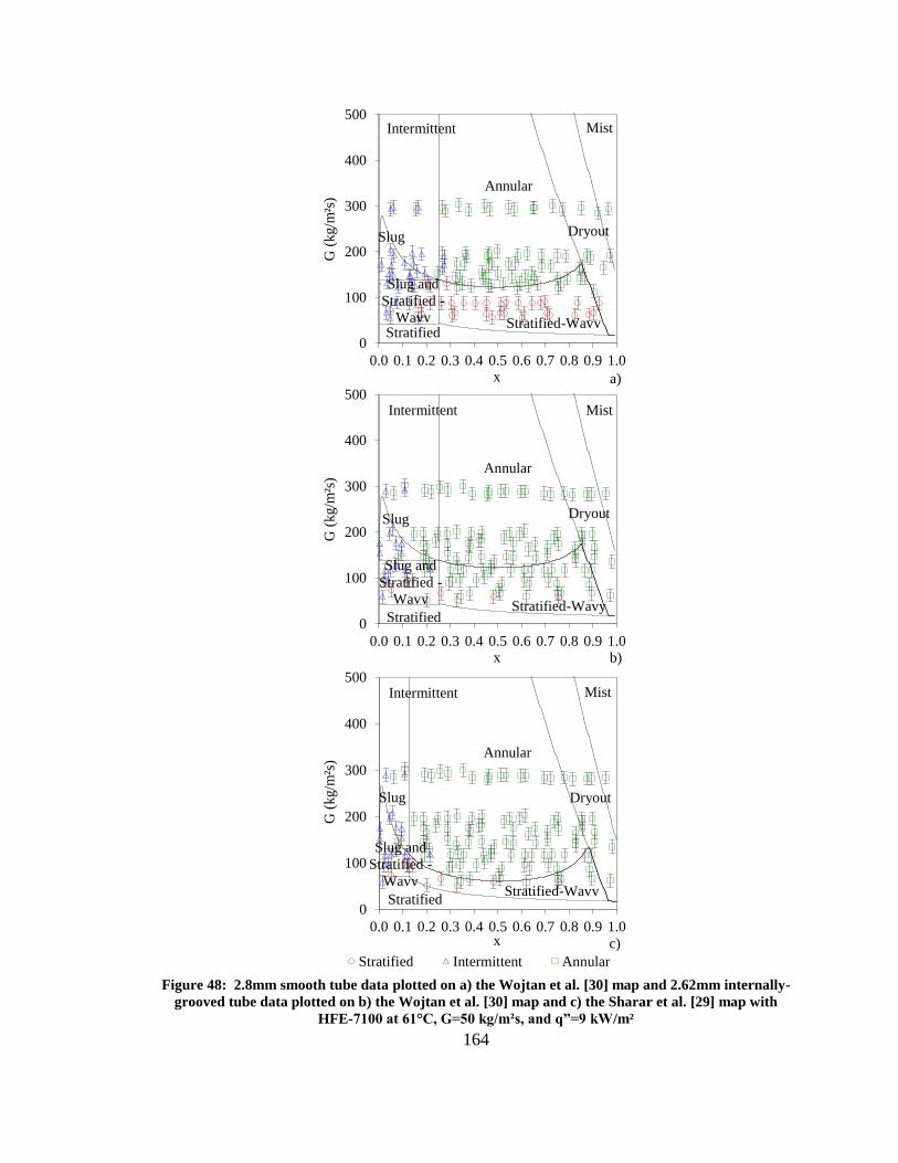
164
Figure 48: 2.8mm smooth tube data plotted on a) the Wojtan et al. [30] map and 2.62mm internally-
grooved tube data plotted on b) the Wojtan et al. [30] map and c) the Sharar et al. [29] map with
HFE-7100 at 61°C, G=50 kg/m²s, and q”=9 kW/m²
0
100
200
300
400
500
0.0 0.1 0.2 0.3 0.4 0.5 0.6 0.7 0.8 0.9 1.0
G (
kg/m
²s)
x
0
100
200
300
400
500
0.0 0.1 0.2 0.3 0.4 0.5 0.6 0.7 0.8 0.9 1.0
G (
kg/m
²s)
x
0
100
200
300
400
500
0.0 0.1 0.2 0.3 0.4 0.5 0.6 0.7 0.8 0.9 1.0
G (
kg/m
²s)
x
Stratified Intermittent Annular
a)
b)
c)
Intermittent
Annular
Slug
Slug and
Stratified -
Wavy Stratified
Stratified-Wavy
Dryout
Mist
Intermittent
Annular
Slug and
Stratified -
Wavy
Stratified Stratified-Wavy
Dryout
Mist
Intermittent
Annular
Slug and
Stratified -
Wavy
Stratified Stratified-Wavy
Dryout
Mist
Slug
Slug

165
It’s also interesting to note that at sufficiently low mass fluxes and vapor qualities,
G<100 kg/m²s and x<0.35, both the smooth and internally-grooved tubes were operating
in Stratified flow. Similarly, at high mass fluxes, G>125 kg/m²s, and high vapor qualities,
x>0.25, both the smooth tube and the internally-grooved tube are operating in Annular
flow. As shown in Figure 48a, the Wojtan et al. [30] flow regime map captures these
smooth tube trends well, however, as shown in Figure 48b it does a poor job predicting
flow regime in the internally-grooved tube; the Wojtan et al. [30] map correctly predicted
131/153 experimental data points for the smooth tube (85.6%) but only 96/153 data points
for the internally-grooved tube (62.7%). The Sharar et al. [29] modified flow regime map
shown in Figure 48c does a good job predicting flow regime in the internally-grooved tube,
correctly predicting 136/153 experimental data points (88.9%). This represents an
improvement of 26.2% by adopting the new Sharar, Bar-Cohen, and Jankowski [29]
modified flow regime map. Again, the model does not predict Annular data points at low
mass flux and high vapor quality, as is the case for 75 kg/m²s and vapor qualities greater
than 0.6.
Figure 49 shows a comparison of experimental heat transfer coefficients for the
smooth and internally-grooved tubes with HFE-7100 at a heat flux of 9 kW/m² for two
mass fluxes; Figure 49a is the lowest mass flux tested for the 2.62-2.8mm tubes (75 kg/m²s)
and Figure 49b is a mass flux of 200 kg/m²s. Mass fluxes below 75 kg/m²s could not be
accurately tested due to the measurement range of the flow meters being used; please refer
to Chapter 5 for more details. The experimental smooth tube data points are shown as red
squares and the internally-grooved tube data points are green circles. The smooth tube heat
transfer coefficient correlation, as described by Wojtan et al. [31], and the internally-

166
grooved tube heat transfer coefficient correlation, described in the current study, are plotted
as solid red and dashed green lines, respectively.
Figure 49: Comparison of heat transfer coefficient vs vapor quality for a mass flux of a) 75 kg/m²s
and b) 200 kg/m²s with HFE-7100 at 61°C and q”=9 kW/m² in 2.62-2.8mm tubes
As can be seen in Figure 49a, the smooth tube heat transfer coefficient remains low
over the full range of vapor qualities tested, for a mass flux of 75 kg/m²s. This is a result
of the prevalence of Stratified flow, as shown in Figure 48a, in the smooth tube and a large
dry perimeter (θdry≠0). Under the same conditions, flow regime transition in the
0
2000
4000
6000
8000
10000
12000
14000
0.0 0.1 0.2 0.3 0.4 0.5 0.6 0.7 0.8 0.9 1.0
Hea
t T
ran
sfer
Co
effi
cien
t (W
/m²K
)
x
0
2000
4000
6000
8000
10000
12000
14000
0.0 0.1 0.2 0.3 0.4 0.5 0.6 0.7 0.8 0.9 1.0
Hea
t T
ran
sfer
Co
effi
cien
t (W
/m²K
)
x0
100020003000400050006000700080009000
10000110001200013000140001500016000170001800019000
0.0 0.1 0.2 0.3 0.4 0.5 0.6 0.7 0.8 0.9 1.0
Current Wojtan IG 1 IG 2 smooth 1 smooth 2
a)
b)
G = 200 kg/m²s, 9 kW/m²
G = 75 kg/m²s, 9 kW/m²
Modified

167
internally-grooved tube has occurred and the enhancement effect is observed. In this case,
the internally-grooved tube enhancement ratio, defined as the grooved tube heat transfer
coefficient divided by the smooth tube coefficient, is close to 5.5; this condition represents
maximum enhancement with the potential for pumping power reduction. It’s interesting
to note that the heat transfer coefficient model over-predicts the heat transfer coefficient at
low vapor quality, x=0.1-0.4. The flow regime map and model predict that the heat transfer
coefficient should increase sharply as the Stratified angle reduces and Annular flow is
approached. Experimentally, however, Stratified flow was maintained and the heat transfer
coefficient remained low until Annular flow was reached at a vapor quality of 0.4.
The trends shown in Figure 49b for a mass flux of 200 kg/m²s are similar to those
for the larger diameter tubes, Figure 43c and Figure 46c. For both the smooth tube and the
internally-grooved tube, the heat transfer coefficients increase monotonically as vapor
quality increases due to the predominance of Annular flow (θdry=0) and a thinning film.
The enhancement factor approaches the area enhancement at a mass flux of 200 kg/m²s
because both tubes are occupying the same flow regime.
The observed and predicted heat transfer coefficients were larger for the 2.62mm
internally-grooved tube and 2.8mm smooth tube than the 8.84mm tubes for similar
operating conditions. As shown in Figure 43c, at a mass flux of 200 kg/m²s, heat flux of 9
kW/m², and vapor quality of 0.7, the smooth tube coefficient was 3172 W/m²K and the
internally-grooved tube coefficient was 7998 W/m²K. For the same conditions (Figure
49b) the 2.8mm smooth tube had a heat transfer coefficient of 4642 W/m²K and the
internally-grooved tube had a coefficient of 9494 W/m²K. This represents a 16% to 32%
improvement by transitioning from an 8.84mm to 2.8mm smooth or 2.62mm internally-

168
grooved tube, respectively. It’s interesting to note that this represents a significant 13%
improvement over the 4.54mm smooth tube but a minor reduction for the internally-
grooved tube performance. Intuitively this makes sense for the smooth tubes whereby a
reduction in tube diameter leads to a thinner film and an increasing heat transfer coefficient.
The seemingly contradictory results in the internally-grooved tube can be explained by
closer inspection of the Ravigururajan and Bergles turbulent enhancement factor Erb
(Equation (36)); the 2.62mm internally-grooved tube has a smaller groove height, smaller
number of fins, and smaller helix angle which reduces the component contributed in
Equation (36) and (37).
8.3.2 Influence of Heat Flux
Figure 50 shows heat transfer coefficient vs vapor quality for the 2.8mm smooth
and 2.62mm internally-grooved tubes for a mass flux of 200kg/ m²s and six different heat
fluxes; Figure 50a is a heat flux of 4 kW/m², Figure 50b is a heat flux of 9 kW/m², Figure
50c is a heat flux of 18 kW/m², Figure 50d is a heat flux of 28 kW/m², Figure 50e is a heat
flux of 40 kW/m², and Figure 50f is a heat flux of 56 kW/m². Please refer to Appendix E
for additional data.
The smooth tube and internally-grooved tube correlations both predict higher heat
transfer coefficients at low vapor quality as the heat flux increases. For example, at a vapor
quality of 0.1 the smooth tube correlation predicts an improvement from 2083 W/m²K to
2928 W/m²K when moving from a heat flux of 4 kW/m² to 56 kW/m² due to nucleate
boiling enhancement. The internally-grooved tube correlation predicts a similar trend and
increases from approximately 4421 W/m²K to 5365 W/m²K with heat fluxes of 4 kW/m²
to 56 kW/m², respectively. This enhancement diminishes at higher vapor quality where

169
nucleate boiling is suppressed and convective vaporization dominates. This can be seen at
a vapor quality of 0.5 on Figure 50a and Figure 50f where the heat transfer coefficient is
approximately 8000 W/m²K for both 4 kW/m² and 56 kW/m² in the internally-grooved
tube. The vapor quality at which dryout occurs decreases with increasing heat flux. The
vapor quality where dryout occurs changes from 0.9 to 0.56 for the smooth and internally-
grooved tube correlations when moving from 4 kW/m² to 56 kW/m².
The Wojtan et al. [31] smooth tube correlation was found to accurately predict the
data for heat fluxes at and below 28 kW/m², with a mean and absolute deviation of 30.74%
and -0.50%, but was less accurate for higher heat flux values of 40 kW/m² and 56 kW/m²,
with a mean and absolute deviation of 43.20% and -43.13%. This trend is similar to what
was observed for the 8.84mm and 4.54mm smooth tubes in Figure 44 and Figure 47,
respectively. This effect is clear at the highest mass flux tested, 56 kW/m², and the full
range of vapor qualities where the measured dependence on heat flux was larger than the
values predicted by the Wojtan et al. [31] correlation, especially at high vapor quality where
the model predicts dryout, but experimentally Annular flow was maintained and the heat
transfer coefficient stayed high. The modified heat transfer correlation developed herein
showed similar results, with a mean and absolute deviation of just 19.45% and -8.68% for
heat fluxes ranging from 4 to 28 kW/m², and deviations of 23.14% and -16.31% for heat
fluxes of 40 and 56 kW/m².

170
Figure 50: Comparison of heat transfer coefficient vs vapor quality for the 2.62-2.8mm tubes with
HFE-7100 at 61°C and a mass flux of 200 kg/m²s for heat fluxes of a) 4 kW/m², b) 9 kW/m², c) 18
kW/m², d) 28 kW/m², e) 40 kW/m², and f) 56 kW/m²
0
2000
4000
6000
8000
10000
12000
14000
0.0 0.1 0.2 0.3 0.4 0.5 0.6 0.7 0.8 0.9 1.0
Hea
t T
ransf
er C
oef
fici
ent
(W/m
²K)
x
0
2000
4000
6000
8000
10000
12000
14000
0.0 0.1 0.2 0.3 0.4 0.5 0.6 0.7 0.8 0.9 1.0
Hea
t T
ransf
er C
oef
fici
ent
(W/m
²K)
x
0
2000
4000
6000
8000
10000
12000
14000
0.0 0.1 0.2 0.3 0.4 0.5 0.6 0.7 0.8 0.9 1.0
Hea
t T
ransf
er C
oef
fici
ent
(W/m
²K)
x
0
2000
4000
6000
8000
10000
12000
14000
0.0 0.1 0.2 0.3 0.4 0.5 0.6 0.7 0.8 0.9 1.0
Hea
t T
ransf
er C
oef
fici
ent
(W/m
²K)
x
0
2000
4000
6000
8000
10000
12000
14000
0.0 0.1 0.2 0.3 0.4 0.5 0.6 0.7 0.8 0.9 1.0
Hea
t T
ransf
er C
oef
fici
ent
(W/m
²K)
x
0
2000
4000
6000
8000
10000
12000
14000
0.0 0.1 0.2 0.3 0.4 0.5 0.6 0.7 0.8 0.9 1.0
Hea
t T
ransf
er C
oef
fici
ent
(W/m
²K)
x0
100020003000400050006000700080009000
10000110001200013000140001500016000170001800019000
0.0 0.1 0.2 0.3 0.4 0.5 0.6 0.7 0.8 0.9 1.0
Current Wojtan IG 1 IG 2 smooth 1 smooth 2
4 kW/m² 9 kW/m²
18 kW/m² 28 kW/m²
40 kW/m² 56 kW/m²
a)
c)
e)
b)
d)
f)
Modified

171
Similar to the 2.0mm smooth tube results and, generally-speaking, the majority of
the results in this chapter, a major source of deviation between the predicted and measured
heat transfer coefficient appears to derive from a mis-prediction of the vapor quality at
which dryout occurs. As shown in Figure 50, the models appear to predict the majority of
the dryout data at heat fluxes at and below 9 kW/m² but generally under predicts the vapor
quality at which dryout occurs for heat fluxes exceeding 18 kW/m². Future studies should
focus on a more comprehensive understanding of dryout conditions in smooth and
internally-grooved tubes.
8.4 Tabulation of Flow Regime Modeling Results
Table 15 shows a full tabulation of the predictive accuracy of the original Wojtan
et al. [30] flow regime map for the 2.80mm, 4.54mm, and 8.84mm smooth tube data shown
in Figure 42a, Figure 45a, and Figure 48a. The left column represents the experimentally
observed flow regime or testing parameter and the next three columns represent the number
of successful predictions and total data points (successful/total) for the three tube diameters
when superimposed on the original Wojtan et al. [30] flow regime map.
As shown in Table 15, and in the previous sections, the Wojtan et al. [30] model
did a very good job predicting Stratified and Intermittent flow in the smooth tubes; in fact,
the traditional flow regime map correctly predicted 296/301 (98.3%) Stratified and
Intermittent data points for the full range tested. However, the Wojtan et al. [30] map was
not able to predict a number of Annular data points near the Stratified-Wavy to Annular
transition. Despite this minor misgiving, the traditional Wojtan et al. [30] flow regime map
correctly predicted 178/197 (90.3%), 145/165 (87.9%), and 131/153 (85.6%) data points

172
for the 8.84mm, 4.54mm, and 2.80mm smooth tubes, respectively. This represents a total
weighted average success rate of 86.2% for all smooth tube data points.
Table 15: Predictive accuracy of Traditional Wojtan et al. [30] flow regime map for the smooth tube
data Fluid HFE-7100 HFE-7100 HFE-7100
Sat. Temp. 61°C 61°C 61°C
Diameter 8.84mm 4.54mm 2.80mm
Model Wojtan Wojtan Wojtan
Stratified 81/83 43/43
54/71
47/47 44/44
54/74
34/34 47/50
50/69 Intermittent
Annular
Total 178/197
90.3%
145/165
87.9%
131/153
85.6% %
Table 16 shows a full tabulation of the predictive accuracy of the original Wojtan
et al. [30] flow regime map and the modified Sharar et al. [29] flow regime map developed
in the current study for the 2.62mm, 4.54mm, and 8.84mm internally-grooved tube data,
as shown in Figure 42b and c, Figure 45b and c, and Figure 48b and c. The left column
represents the experimentally observed flow regime or testing parameter and the next six
columns represent the number of successful predictions and total data points
(successful/total) for the three tube diameters when superimposed on the original Wojtan
et al. [30] flow regime map and the modified Sharar et al. [29] map. As shown in Table
16 and in the previous sections, the Wojtan et al. [30] model generally did a poor job
predicting the flow regime in the internally-grooved tubes. The predictive accuracy for
Stratified and Intermittent flow was generally good, but the Wojtan et al. [30] map
predicted only 58/122, 65/112, and 52/109 Annular data points for the 8.84mm, 4.54mm,
and 2.62mm internally-grooved tubes, respectively. This represents a 51.0% predictive
accuracy of Annular flow in internally-grooved tubes using the traditional Wojtan et al.
[30] flow regime map and a total weighted average success rate 66.7% for all data points.

173
Table 16: Predictive accuracy of Traditional Wojtan et al. [30] and Modified Sharar et al. [29] flow
regime maps for the internally-grooved tube data Fluid HFE-7100 HFE-7100 HFE-7100
Sat. Temp. 61°C 61°C 61°C
Diameter 8.84mm 4.54mm 2.62mm
Model Wojtan Modified Wojtan Modified Wojtan Modified
Stratified 34/34 31/34 25/25 19/25 8/8 8/8
Intermittent 30/30 28/30 29/29 29/29 36/36 35/36
Annular 58/122 105/122 65/112 95/112 52/109 93/109
Total 122/186 164/186 119/166 143/166 96/153 136/153
% 65.6% 87.7% 71.7% 86.1% 62.7% 88.9%
The new model, applied to the internally-grooved tubes, did not always improve
the success of predicting Stratified and Intermittent flow compared to the Wojtan et al. [30]
flow regime map. A minor reduction from 34/34 to 31/34 Stratified data points for the
8.84mm tube and 25/25 to 19/25 Stratified data points for 4.54mm tube was observed.
Similarly, a minor reduction from 30/30 to 28/30 Intermittent data points for the 8.84mm
tube, and 36/36 to 35/36 Intermittent data points for the 2.62mm tube was shown.
However, the new model significantly improves the predictability for Annular flow in all
of the studies. The new model improved Annular flow predictive accuracy from 58/122 to
105/122 for the 8.84mm tube, 65/112 to 95/112 for the 4.54mm tube, and 52/109 to 93/109
for the 2.62mm tube; this represents and improvement of 34.4% in predicting Annular
flow, from 51.0% accuracy to 85.4%, by adopting the new model. Overall, the new model
represents an improvement from 66.7% accuracy for the Wojtan et al. [30] model to 88.3%
using the updated transition criteria. Based on these results, the new model appears to far
more accurately predict early transition to Annular flow for the current data set.
8.5 Enhancement Ratio
Figure 51 shows a graphical summary of the enhancement ratio vs mass flux based
on Figure 43, Figure 46, Figure 49, and additional 9 kW/m² data from Appendix C -

174
Appendix E. This is similar to the figure shown in the Chapter 4 summary of the simulated
modeling results and is revisited here with superimposed experimental data.
Figure 51: Enhancement ratio vs mass flux with current data for the 8.84mm, 4.54mm, and 2.62mm
internally-grooved tubes
The blue dashed line represents the predicted enhancement ratios for a vapor quality
of 0.45 to 0.55 for the specific geometric parameters of the 8.84mm tube and plotted as a
function of mass flux; again, the enhancement ratio is defined as the internally-grooved
tube heat transfer coefficient divided by the smooth tube heat transfer coefficient.
0
1
2
3
4
5
6
7
8
0 100 200 300 400
Enhan
cem
ent
Rat
io
G (kg/m²s)
Enhancement Ratio Area Enhancement 8.84mm 4.54mm 2.62mm
x=0.45 – 0.55
Figure
43a
Figure
43b
Figure
43c
Figure
46c
Figure
46b
Figure
46a
Figure
49a
Figure
49b
8.84/4.54mm
enhancement ratio
2.62mm
enhancement ratio

175
Specifically, this was calculated with HFE-7100 at a saturation temperature of 61°C in an
8.84mm tube with an area enhancement of 1.52, fin height of 0.2mm, and a helix angle of
18°; a similar enhancement ratio was predicted for the 4.54mm tubes and was not included
here for figure clarity. The dashed green line is the predicted enhancement ratio for the
2.62mm internally-grooved tube; this was calculated for HFE-7100 at a saturation
temperature of 61°C in an 2.62mm tube with an area enhancement of 1.6, fin height of
0.12mm, and a helix angle of 10° Horizontal error bars for the uncertainty in mass flux
are shown. Additionally, labels for several data points direct the reader back to
corresponding figures earlier in this chapter.
The figure shows heat transfer improvement approximately equal to the area ratio
of 1.52 at sufficiently low mass flux where both the smooth and internally-grooved tubes
were operating in Stratified or Stratified-Wavy flow; this was the case for the 8.84mm
smooth and internally-grooved tube at 9 kW/m² and a mass flux of 25 kg/m²s, as shown in
Figure 43a. The enhancement ratio also approached the area enhancement at high mass
flux where both tubes were operating in the Slug, Intermittent, or Annular flow regime and
the dry angle was zero (θdry=0); this can be clearly seen in Figure 43c, Figure 44b, Figure
46c, Figure 47b, Figure 49b, and Figure 50b. Large enhancement (5 to 7x) was predicted
at low-to-intermediate mass fluxes where the smooth tube was operating in Stratified flow
and the internally-grooved tube is operating in Annular flow; this was shown for the
8.84mm, 4.54mm, and 2.62mm internally-grooved tubes in Figure 43b, Figure 46a, Figure
46c, and Figure 49a. These trends are consistent with those described earlier and indicate
that the new flow regime map and associated heat transfer coefficient can capture the
physical mechanisms responsible for enhancement in internally-grooved tubes.

176
As shown in Figure 51, different tube geometric parameters (and fluids) result in
different predicted enhancement ratios. Therefore, applying these exact predictions to
different working fluids, saturation temperatures, and geometric parameters has
limitations. Clearly, these parameters can affect the mass flux at which flow regime
transition occurs and the relative effect of turbulence, Equation (36), and wet angle heat
transfer coefficient, Equation (37). For example, the 2.62mm internally-grooved tube has
a smaller helix angle (10° vs 18º), less fins (36 vs 60), and a smaller fin height (0.12mm vs
0.20mm) compared to the 8.84mm and 4.54mm internally-grooved tubes. This results in
a reduction from 1.38 to 1.14 in the turbulence factor proposed by Ravagururajan and
Bergles [28], and a corresponding reduction on Figure 51.
8.6 Statistical Assessment of the Heat Transfer Coefficient Correlations
In this section, several smooth tube and internally-grooved tube heat transfer
coefficient models will be evaluated using the experimental database gathered in the
current study for 2.8/2.62mm, 4.54mm, and 8.84mm tubes with heat fluxes from 4 kW/m²
to 56 kW/m², mass fluxes ranging from 25 to 300 kg/m²s, and HFE-7100 at 61ºC as the
working fluid. Graphs for the largest diameter, 8.84mm, will be shown below and a tabular
summary of all results will be provided. Please refer to Appendix F for similar figures for
the 4.54mm and 2.62/2.8mm smooth and internally-grooved tubes, and a more detailed
table of results. Please note, the figures created only consider ‘IG 1’ and ‘smooth 1’ data
points which are fully representative of the trends observed for ‘IG 2’ and ‘smooth 2’; this
allowed figure clarity. The summary tables, however, considered all of the experimental
data. The statistical parameters of mean deviation, 𝜀, and mean of absolute value of
deviations, |𝜀|, were calculated based on the equations below:

177
ε = ∑[(hpredicted − hexperimental)100/hexperimental] (70)
|ε| = ∑ ABS[(hpredicted − hexperimental)100/hexperimental] (71)
where hpredicted is the heat transfer coefficient predicted by the respective heat transfer
coefficient correlation and hexperimental is the measured heat transfer coefficient. These
parameters are used to assess the success of the models in context of mass flux and flow
regime.
8.6.1 Smooth Tubes
Measured smooth tube heat transfer coefficients were compared to the smooth tube
two-phase correlations of Wojtan et al. [31], Chen [56], Shah [57], Kandlikar [93], Gungor
and Winterton [59], and a simplified two-phase flow boiling correlation by Gungor and
Winterton [60] (referred to hereafter as Gungor-Winterton ‘new’). Figure 52 shows the
predicted heat transfer coefficient values vs the experimental two-phase heat transfer
coefficient values for different mass fluxes. The solid black line has a slope of 1, indicating
perfect agreement between the model and experimental results. The dashed lines represent
±20% for reference. The properties used while evaluating these correlations were the
average values between the inlet and outlet of the test section (at the location of the wall
temperature measurements). Table 17 lists a summary of the statistical parameters for the
six correlations used.

178
Figure 52: Comparison of the 8.84mm smooth tube experimental data for HFE-7100 at 61°C with
correlations from a) Wojtan et al. [31], b) Chen [56], c) Shah [57], d) Kandlikar [93], e) Gungor-
Winterton ‘original’ [59], and f) Gungor-Winterton ‘new’ [60]
0
1000
2000
3000
4000
5000
0 1000 2000 3000 4000 5000
h W
ojt
an (
W/m
²K)
h exp. (W/m²K)
0
1000
2000
3000
4000
5000
0 1000 2000 3000 4000 5000
h C
hen
(W
/m²K
)
h exp (W/m²K)
0
1000
2000
3000
4000
5000
0 1000 2000 3000 4000 5000
h S
hah
(W
/m²K
)
h exp (W/m²K)
0
1000
2000
3000
4000
5000
0 1000 2000 3000 4000 5000
h K
and
likar
(W
/m²K
)
h exp (W/m²K)
0
1000
2000
3000
4000
5000
0 1000 2000 3000 4000 5000
h G
ungo
r-W
inte
rto
n (
W/m
²K)
h exp (W/m²K)
0
1000
2000
3000
4000
5000
0 1000 2000 3000 4000 5000
h G
ungo
r-W
inte
rto
n n
ew (
W/m
²K)
h exp. (W/m²K)
0
1000
2000
3000
4000
5000
6000
7000
8000
9000
10000
0 2000 4000 6000 8000 10000
h p
red
(W
/m²K
)
h exp (W/m²K)
G300 G200 G175 G150 G125 G100 G75 G50 G25
a) b)
c) d)
e) f)
f
x=0.82
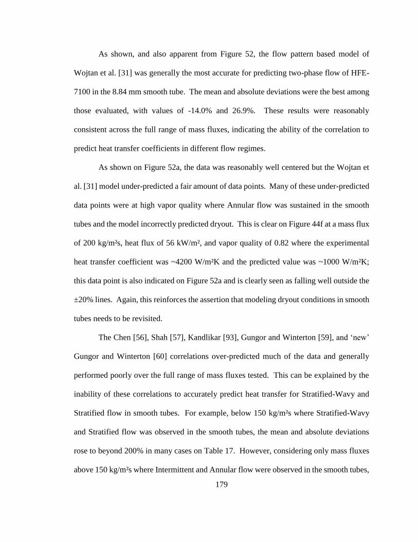
179
As shown, and also apparent from Figure 52, the flow pattern based model of
Wojtan et al. [31] was generally the most accurate for predicting two-phase flow of HFE-
7100 in the 8.84 mm smooth tube. The mean and absolute deviations were the best among
those evaluated, with values of -14.0% and 26.9%. These results were reasonably
consistent across the full range of mass fluxes, indicating the ability of the correlation to
predict heat transfer coefficients in different flow regimes.
As shown on Figure 52a, the data was reasonably well centered but the Wojtan et
al. [31] model under-predicted a fair amount of data points. Many of these under-predicted
data points were at high vapor quality where Annular flow was sustained in the smooth
tubes and the model incorrectly predicted dryout. This is clear on Figure 44f at a mass flux
of 200 kg/m²s, heat flux of 56 kW/m², and vapor quality of 0.82 where the experimental
heat transfer coefficient was ~4200 W/m²K and the predicted value was ~1000 W/m²K;
this data point is also indicated on Figure 52a and is clearly seen as falling well outside the
±20% lines. Again, this reinforces the assertion that modeling dryout conditions in smooth
tubes needs to be revisited.
The Chen [56], Shah [57], Kandlikar [93], Gungor and Winterton [59], and ‘new’
Gungor and Winterton [60] correlations over-predicted much of the data and generally
performed poorly over the full range of mass fluxes tested. This can be explained by the
inability of these correlations to accurately predict heat transfer for Stratified-Wavy and
Stratified flow in smooth tubes. For example, below 150 kg/m²s where Stratified-Wavy
and Stratified flow was observed in the smooth tubes, the mean and absolute deviations
rose to beyond 200% in many cases on Table 17. However, considering only mass fluxes
above 150 kg/m²s where Intermittent and Annular flow were observed in the smooth tubes,

180
the models performed reasonably well. For example, the Chen [56] correlation showed a
mean and absolute deviation of only 4.5% and 25.2% for the mass flux of 300 kg/m²s where
Annular flow was the dominant flow regime and 679% mean and absolute error for a mass
flux of 25 kg/m²s where Stratified flow dominated. It’s worth noting that, as repeatedly
observed by Rahim, Bar-Cohen, et al. [35] [55], the Chen [56] correlation performs
remarkably well in the Annular flow regime and actually outperformed the Wojtan et al.
[31] correlation at 300 kg/m²s. Similar trends can be seen for the Shah [57], Kandlikar
[93], Gungor-Winterton [59], and ‘new’ Gungor-Winterton [60] correlations.
Table 17: Predictive accuracy of two-phase smooth tube heat transfer coefficient correlations from
Wojtan et al. [31], Chen [56], Shah [57], Kandlikar [93], and Gungor-Winterton [59] [60]
compared to the 2.8mm to 8.84mm experimental results
G
kg/m²s
Wojtan % Chen % Shah % Kandlikar % Gungor-
Winterton %
Gungor-
Winterton
new %
𝜺 |𝜺| 𝜺 |𝜺| 𝜺 |𝜺| 𝜺 |𝜺| 𝜺 |𝜺| 𝜺 |𝜺|
300 -13.1 25.0 4.5 25.2 9.67 31.6 96.2 97.5 15.3 40.3 3.3 34.4
200 -12.9 25.0 15.2 30.3 26.4 42.7 68.5 69.7 25.8 45.5 5.7 34.0
175 -13.7 25.6 24.6 37.4 34.8 52.5 60.9 63.5 34.1 54.1 9.6 38.9
150 -12.9 22.6 28.6 42.7 34.2 53.3 47.9 56.2 36.1 57.3 8.9 39.2
125 -13.5 24.4 54.4 59.8 56.4 64.8 56.5 59.1 61.8 71.7 26.1 42.2
100 -18.7 32.8 110.3 153.0 106.5 116.5 86.8 97.6 118.8 132.5 65.2 78.8
75 -10.2 28.3 274.1 274.1 200.7 200.8 130.8 131.9 204.2 204.3 134.3 134.6
50 -8.6 33.6 487.2 488.4 277.1 277.1 156.8 157.3 214.4 214.4 216.7 216.7
25 -47.3 47.9 679.1 679.1 98.8 98.8 59.0 63.6 88.7 90.7 157.0 157.0
total -14.0 26.9 100.7 115.6 72.8 85.9 80.6 84.4 72.1 87.5 44.3 65.3
8.6.2 Internally-Grooved Tubes
Measured internally-grooved tube heat transfer coefficients were compared to the
current two-phase correlation described in Chapter 4, and the correlations of Thome,
Kattan, and Favrat [91], Cavallini et al. [117], Chamra and Mago [162], Wu et al. [103],
and Yun et al. [90]. Figure 53 shows the predicted heat transfer coefficient values vs the
experimental two-phase heat transfer coefficient values for different mass fluxes. Again,
the solid black line has a slope of 1 indicating perfect agreement between the model and
experimental results and the dashed lines represent ±20% deviation.
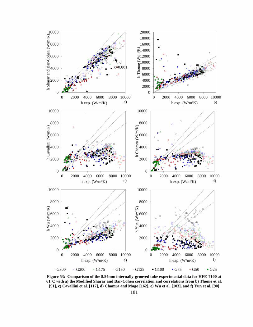
181
Figure 53: Comparison of the 8.84mm internally-grooved tube experimental data for HFE-7100 at
61°C with a) the Modified Sharar and Bar-Cohen correlation and correlations from b) Thome et al.
[91], c) Cavallini et al. [117], d) Chamra and Mago [162], e) Wu et al. [103], and f) Yun et al. [90]
0
2000
4000
6000
8000
10000
0 2000 4000 6000 8000 10000
h S
har
ar a
nd
Bar
-Co
hen
(W
/m²K
)
h exp. (W/m²K)
0
2000
4000
6000
8000
10000
12000
14000
16000
18000
20000
0 2000 4000 6000 8000 10000
h T
ho
me
(W/m
²K)
h exp. (W/m²K)
0
2000
4000
6000
8000
10000
0 2000 4000 6000 8000 10000
h C
aval
lini
(W/m
²K)
h exp. (W/m²K)
0
2000
4000
6000
8000
10000
0 2000 4000 6000 8000 10000
h C
ham
ra (
W/m
²K)
h exp. (W/m²K)
0
2000
4000
6000
8000
10000
0 2000 4000 6000 8000 10000
h W
u (
W/m
²K)
h exp. (W/m²K)
0
2000
4000
6000
8000
10000
0 2000 4000 6000 8000 10000
h Y
un (
W/m
²K)
h exp. (W/m²K)
0
1000
2000
3000
4000
5000
6000
7000
8000
9000
10000
0 2000 4000 6000 8000 10000
h p
red
(W
/m²K
)
h exp (W/m²K)
G300 G200 G175 G150 G125 G100 G75 G50 G25
a) b)
c) d)
e) f)
d
x=0.801

182
Table 18 lists a summary of the statistical parameters for the six internally-grooved
correlations used. The mean deviation was best for the Wu et al. [103] correlation with a
value of -2.4%, indicating that the data was ‘well centered’. However, the absolute error
was quite high with a value of 80.7%. The large absolute deviation is clear from Figure
53e. The small mean deviation, therefore, is a result of the large errors at high predicted
values and low experimental values that offset the general trend of under-predicting heat
transfer coefficient. The same assessment can be made for the Cavallini et al. [117],
Chamra and Mago [162] correlations.
Table 18: Predictive accuracy of Modified Sharar and Bar-Cohen two-phase internally-grooved tube
heat transfer coefficient correlation and correlations from Thome et al. [91], Cavallini et al. [117],
Chamra and Mago [162], Wu et al. [103], and Yun et al. [90]
G Modified % Thome % Cavallini % Chamra % Wu % Yun %
kg/m²s 𝜺 |𝜺| 𝜺 |𝜺| 𝜺 |𝜺| 𝜺 |𝜺| 𝜺 |𝜺| 𝜺 |𝜺|
300 -5.1 28.7 52.8 61.5 -23.4 44.0 30.0 91.3 -1.0 58.5 -35.7 55.3
200 1.1 25.1 67.3 74.7 -19.3 47.9 -10.9 55.9 -11.1 73.2 -55.9 68.3
175 11.2 31.3 82.0 87.3 -10.4 54.3 -5.6 61.4 -11.5 76.2 -63.7 70.1
150 21.7 40.9 99.5 105.0 -3.7 59.5 36.9 104.6 -8.9 84.0 -63.9 74.4
125 10.8 29.1 93.6 98.7 -0.7 60.9 -1.1 66.3 -17.7 77.1 -64.7 77.9
100 3.6 31.0 196.3 202.8 18.8 77.4 30.8 97.2 18.9 111.8 -70.7 76.4
75 -2.8 31.7 130.3 135.0 82.3 129.6 65.1 123.1 -16.1 73.8 -60.6 80.6
50 -12.9 41.1 250.7 252.3 76.6 119.2 75.8 132.5 22.6 95.5 -55.1 79.9
25 -21.3 48.9 530.3 530.3 210.7 223.9 129.7 152.9 112.4 133.7 -48.3 73.0
total 4.0 32.0 118.7 124.6 12.6 72.3 25.4 88.9 -2.4 80.7 -58.2 71.85
The Thome et al. [91], Cavallini et al. [117], Chamra and Mago [162], Wu et al.
[103], and Yun et al. [90] correlations generally performed poorly over the full range of
mass fluxes tested but worked markedly better for higher mass fluxes. Similar to the
smooth tube correlations, this is explained by the inability of these correlations to
accurately predict heat transfer for Stratified-Wavy (Slug and Stratified-Wavy) and
Stratified flow. For example, below 150 kg/m²s on Figure 42c, where Stratified flow was
observed in the internally-grooved tubes, the mean and absolute deviations rose to values
in excess of 100% in many cases on Table 18. At and below mass fluxes of 75 kg/m²s,

183
where Stratified flow occupied 40% or 100% of the parametric space, deviations further
increased. However, considering only mass fluxes above 150 kg/m²s where Intermittent
and Annular flow were the dominant flow regimes in the internally-grooved tubes, some
of the models performed reasonably well. For example, the Cavallini et al. [117]
correlation showed a mean and absolute deviation of -23.4% and 44.0% for the mass flux
of 300 kg/m²s where Annular flow was the dominant flow regime and 210.7% to 223.9%
mean and absolute error for a mass flux of 25 kg/m²s where Stratified flow dominated.
From a practical standpoint, the model developed in this Dissertation was the best
among those evaluated with a mean deviation of 4% and a relatively low absolute deviation
of 32%. These results were reasonably consistent across the full range of mass fluxes,
indicating the ability of the correlation to predict heat transfer coefficients in different flow
regimes. As shown on Figure 53a, the data was reasonably well centered but under-
predicted a substantial number of data points. Many of these under-predicted data points
were at high vapor quality where Annular flow was sustained in the internally-grooved
tubes and the model incorrectly predicted dryout; this effect was also noted for the smooth
tube data and indicates the need to re-examine dryout conditions in smooth and internally-
grooved tubes in the future. This is clear on Figure 44d at a mass flux of 200 kg/m²s, heat
flux of 28 kW/m², and vapor quality of 0.801 where the experimental heat transfer
coefficient was ~8300 W/m²K and the predicted value was ~5500 W/m²K; this data point
is also indicated on Figure 53a and is clearly seen as falling well outside the ±20% lines.
It was also found that data around 50 kg/m²s (more so for the 8.84mm tube than the
4.54mm tube) deviated from the new model value more than other mass fluxes, as shown
on Figure 53a. It is speculated that this is a result of experimental uncertainty in mass flux.

184
The mass flux experimental uncertainty was a fixed value of ±10.5 kg/m²s for the 8.84mm
tubes. Therefore, at a mass flux of 50 kg/m²s, the actual mass flux could, in fact, be
operating anywhere from 40 kg/m²s to 60 kg/m²s. Figure 54 shows an example of how
much the heat transfer coefficient can be expected to change for mass fluxes ranging from
40 kg/m²s to 60 kg/m²s based on the heat transfer model described herein. Figure 54a is
the Modified Sharar et al. [29] flow regime map for HFE-7100 in an 8.84mm internally-
grooved tube superimposed with the loci of 40 kg/m²s, 50 kg/m²s, and 60 kg/m²s; they are
shown as a blue dashed line, green dashed line, and red dashed line, respectively. Figure
54b is the simulated heat transfer coefficient, for the same mass fluxes, along with the
smooth tube data and internally-grooved tube data at a mass flux of 50 kg/m²s and
equivalent heat flux.
Figure 54: Example of heat transfer coefficient uncertainty and deviation near the transition
boundary between Stratified-Wavy and Annular flow for HFE-7100 at 61°C in the 8.84mm tubes; a)
locus of different flowrates on the Modified flow regime map and b) resulting heat transfer
coefficients
As can be seen from Figure 54a, at a mass flux of 50 kg/m²s the tube is expected to
be operating in Stratified flow at low vapor quality, then transition to Stratified-Wavy flow
0
100
200
300
400
500
0.0 0.1 0.2 0.3 0.4 0.5 0.6 0.7 0.8 0.9 1.0
G (
kg/m
²s)
x
0
1000
2000
3000
4000
5000
0.0 0.1 0.2 0.3 0.4 0.5 0.6 0.7 0.8 0.9 1.0
Hea
t T
ransf
er C
oef
fici
ent
(W/m
²K)
x
02000400060008000
0.0 0.1 0.2 0.3 0.4 0.5 0.6 0.7 0.8 0.9 1.0
Hea
t T
ransf
er C
oef
fici
ent
(W/m
²K)
x
Current 40 kg/ms Current 50 kg/ms Current 60 kg/ms WojtanIG 1 IG 2 smooth 1 smooth 2
Intermittent
Annular
Slug and
Stratified -
Wavy
Stratified Stratified-Wavy
Dryout
Mist
Slug
Modified 40 kg/m²s Modified 50 kg/m²s Modified 60 kg/m²s
a) b)
50 kg/m²s

185
at a vapor quality of 0.2, and approach Annular flow around a vapor quality of 0.7. The
result, as seen on Figure 54b, is a relatively low heat transfer coefficient until Stratified-
Wavy flow is reached, and a maximum heat transfer coefficient of 3032 W/m²K at x=0.7,
where Annular flow is approached and the dry angle is small; the model at this mass flux
under-predicts the experimental data. At a lower mass flux of 40 kg/m²s, where the model
predicts Stratified and Stratified-Wavy flow, the heat transfer coefficient is worse-still due
to a larger dry angle. In this case, the maximum heat transfer coefficient is only 2182
W/m²K, representing a 28% reduction in predicted performance from 50 kg/m²s; the model
under-predicts the experimental data at 40 kg/m²s. At a higher mass flux of 60 kg/m²s, the
flow regime starts as Stratified and Stratified-Wavy flow but transitions to Annular flow at
a vapor quality of 0.49. This results in a much larger predicted heat transfer coefficient
(maximum value of 4869 W/m²K), representing a 37% and 55% improvement over the
predicted values for 40 kg/m²s and 50 kg/m²s, respectively. As shown, the predicted values
at 40 and 50 kg/m²s tend to under-predict the measured values at 50 kg/m²s, but the 60
kg/m²s model simulation generally over-predicts the experimental results. This validates
the argument that uncertainty in the experimental mass flux and proximity to the Stratified-
Wavy to Annular transition line is the likely explanation of the large deviation at a mass
flux of 50 kg/m²s. Future work should focus on improving the test facilities to reduce mass
flux uncertainty and allow a more robust understanding and discussion of heat transfer
around the Stratified-Wavy to Annular transition line.
It’s interesting to note that the mass flux uncertainty may also explain variation
between the predicted and measured enhancement ratio shown in Figure 51. As shown, a
seemingly modest uncertainty of ±10.5 kg/m²s can result in large deviations in the

186
enhancement ratio because the slope of enhancement vs mass flux is very steep in the
Stratified-Wavy to Annular transition region. Again, efforts should be made to reduce the
uncertainty in the experimental mass flux to better map out the enhancement vs mass flux
chart shown in Figure 51.
8.7 Comparison to Data from the Literature
The studies from Yu et al. [66], Colombo et al. [79], and Spindler and Müller-
Steinhagen [74], discussed in Chapter 3, demonstrated the shift of the dominant Annular
flow regimes in internally-grooved tubes to lower mass flux and vapor quality and an
expansion of the parametric space occupied by Annular flow. The traditional Wojtan et al.
[30] map did a poor job predicting flow regimes in these studies due to the observed flow
regime transition; this conclusion from the literature review was a driving factor in
undertaking the current research effort. The goal of this section is to revisit those studies
and compare their flow regime and heat transfer coefficient data to the new flow regime
map and regime based heat transfer coefficient correlation. This serves several purposes;
a) further substantiate early flow regime transition to Annular flow as an enhancement
mechanism in internally-grooved tubes; b) provide an independent validation of the flow
regime map and heat transfer coefficient developed Chapter 4.
8.7.1 Flow Regime Data
Yu, Lin, and Tseng [66] performed a flow visualization and heat transfer study with
R134a at 6ºC in a 10.7 mm ID smooth and an 11.1 mm ID internally-grooved tube with an
18° helix angle. Mass fluxes from 163 to 408 kg/m²s, heat flux between 2.2 and 56 kW/m²,
and a fixed heated length of 1.5 m were tested. Figure 55a shows the results of the
internally-grooved tube flow visualization, plotted in the coordinates of mass flux and

187
vapor quality and superimposed on the Wojtan et al. [30] flow regime map and modified
Sharar et al. [29] map; Figure 55a is the data plotted on the Wojtan et al. [30] map and
Figure 55b is the internally-grooved tube results plotted on the Sharar et al. [29] map. As
shown in Figure 55a, the Wojtan et al. [30] flow regime map predicted 45/47 Intermittent
data points but only 6/30 Annular flow data points for the Yu et al. [66] internally-grooved
tube. In total, the Wojtan et al. [30] flow regime map predicted 51/77 experimental data
points, equaling 66% of the internally-grooved tube data. As shown in Figure 55b, the
current flow regime modifications, which shift Annular flow to lower vapor quality and
mass flux, greatly improved the predictive accuracy for the Yu et al. [66] internally-
grooved tube data. The new model predicted 43/47 Intermittent data points and 21/30
Annular data points; this is a weighted average total of 83% of the data from Yu et al. [66].
Figure 55: 11.1 mm ID internally-grooved tube experimental flow visualization results from Yu et al.
[66] for R134a at 6ºC with a heat flux of 20 kW/m² plotted on the a) original Wojtan et al. [30] map
and b) Modified Sharar et al. [29] map
Colombo et al. [79] performed a flow visualization and evaporative heat transfer
study with R134a at a saturation temperature of 5°C in a horizontal 8.92 mm ID smooth
0
100
200
300
400
500
0 0.1 0.2 0.3 0.4 0.5 0.6 0.7 0.8 0.9 1
G (
kg/m
²s)
x
0
100
200
300
400
500
0 0.1 0.2 0.3 0.4 0.5 0.6 0.7 0.8 0.9 1
G (
kg/m
²s)
x
1 1 1
Intermittent
Annular
Stratified
Slug and
Stratified-
Wavy
Slug
Stratified-Wavy
Dryout
Mist Intermittent
Annular
Stratified
Slug and
Stratified-
Wavy
Slug
Stratified-Wavy
Dryout
Mist
(a) (b)
Annular Intermittent

188
tube and two internally-grooved tubes with inside diameters of 8.62 and 8.92 mm. Both
internally-grooved tubes had helix angles of 18° and apex angles of 40º but had alternating
fin heights ranging from 0.16 to 0.23 mm and the number of grooves ranging from 54 to
82. The resulting internally-grooved tube area ratio ranged from 1.55 to 1.82. Mass fluxes
from 100 to 340 kg/m²s, heat flux between 2.2 and 56 kW/m², vapor qualities from 0.1 to
0.9, and a fixed heated length of 1.3 m were tested.
Figure 56 shows the results of the flow visualization, plotted in the coordinates of
mass flux and vapor quality and superimposed on the Wojtan et al. [30] flow regime map
and Sharar et al. [29] map; Figure 56a is the internally-grooved tube experimental results
on the traditional map [30] and Figure 56b is the same results on the new model [29]
described herein. As shown, the modified map markedly improves predictability of flow
regime in the internally-grooved tube, particularly for Annular flow. Compared to the
smooth tube model, Figure 56a, which predicted 31/31 Stratified data points, 2/4
Intermittent data points, and only 25/42 Annular data points, the new model, Figure 56b,
predicted 28/31 Stratified data points, 0/4 Intermittent data points, and 42/42 Annular data
points. This represents an improvement from 75% to 91% predictive accuracy when
switching from the Wojtan et al. [30] model to the new Sharar et al. [29] model.
Spindler and Müller-Steinhagen [74] performed an experimental investigation of
heat transfer and flow regime during evaporative cooling in an 8.92 mm ID internally-
grooved tube with a 15° helix angle using two different refrigerants, R134a and R404A.
Experiments were conducted in a 1 m long, heated test section with mass fluxes ranging
from 25 to 150 kg/m², heat flux from 1 to 15 kW/m², inlet vapor qualities ranging from 0.1
to 0.7, and a saturation temperature of -20ºC. Stratified, Intermittent, and Annular flow

189
were observed, however, Annular flow was the dominant regime for mass fluxes at or
above 65 kg/m²s.
Figure 56: 8.92 mm ID internally-grooved tube experimental flow visualization results from
Colombo et al. [79] with R134a at 5ºC and a heat flux of 4.2 kW/m² plotted on the a) original Wojtan
et al. [30] map and b) Modified Sharar et al. [29] map
Figure 57a and Figure 57b show the R134a internally-grooved tube data of Spindler
and Müller-Steinhagen [74] plotted on the traditional flow regime map [30] and the
modified map [29], respectively. Similar to Figure 55 and Figure 56 above, the modified
map improves predictability of flow regime in the internally-grooved tube. The smooth
tube Wojtan et al. [30] model, Figure 57a, predicted 2/3 Stratified data points and 3/11
Annular data points while the new model [29], Figure 57b, predicted 2/3 Stratified data
points and 9/11 Annular data points. This represents an improvement from 36% predictive
accuracy to 79% accuracy.
0
100
200
300
400
500
0 0.1 0.2 0.3 0.4 0.5 0.6 0.7 0.8 0.9 1
G (
kg/m
²s)
x
0
100
200
300
400
500
0 0.1 0.2 0.3 0.4 0.5 0.6 0.7 0.8 0.9 1
G (
kg/m
²s)
x
1 1 1
Intermittent
Annular
Stratified
Slug and
Stratified-
Wavy
Slug
Stratified-Wavy
Dryout
Mist
(a)
Intermittent
Annular
Stratified
Slug and
Stratified-
Wavy
Slug
Stratified-Wavy
Dryout
Mist
(b)
Stratified Annular Intermittent

190
Figure 57: 8.92 mm ID internally-grooved tube experimental flow visualization results from
Spindler and Müller-Steinhagen [74] for R134a at -20ºC with a heat flux of 7.5 kW/m² plotted on the
a) original Wojtan et al. [30] map and b) Modified Sharar et al. [29] map
Figure 58 shows the R404a internally-grooved tube data of Spindler and Müller-
Steinhagen [74] plotted on the traditional [30] and modified Sharar et al. [29] flow regime
maps. As is consistent with the above results, the modified model greatly improved
predictive accuracy for the data set. The original model correctly predicted 2/3 Stratified
data points but only 3/11 Annular data points while the modified model predicted 2/3
Stratified data points and a much improved 10/11 Annular data points. The represents an
overall accuracy improvement of 49%, from 36% for the Wojtan et al. [30] model (only
5/14 correct) to 85% for the Sharar et al. [29] model (12/14 correct).
0
100
200
300
400
500
0 0.1 0.2 0.3 0.4 0.5 0.6 0.7 0.8 0.9 1
G (
kg/m
²s)
x
0
100
200
300
400
500
0 0.1 0.2 0.3 0.4 0.5 0.6 0.7 0.8 0.9 1
G (
kg/m
²s)
x
1 1 1
Intermittent
Annular
Stratified
Slug and
Stratified-
Wavy
Slug
Stratified-Wavy
Dryout
Mist
(a)
Intermittent
Annular
Stratified
Slug and
Stratified-
Wavy
Slug
Stratified-Wavy
Dryout
Mist
(b)
Stratified Annular

191
Figure 58: 8.92 mm ID internally-grooved tube experimental flow visualization results from
Spindler and Müller-Steinhagen [74] for R404a at -20ºC with a heat flux of 7.5 kW/m² plotted on the
a) original Wojtan et al. [30] map and b) Modified Sharar et al. [29] map
A full tabulation of the success of the original Wojtan et al. [30] and modified
Sharar et al. [29] flow regime maps are shown in Table 19. The left column represents the
experimentally observed flow regime or testing parameters and the next 8 columns
represent the number of successful predictions and total data points (successful/total) for
the Yu et al. [66], Colombo et al. [79], and Spindler and Müller-Steinhagen [74] studies
when superimposed on the traditional Wojtan et al. [30] and modified Sharar et al. [29]
models. As shown, the modified model outperforms the traditional model for predicting
flow regime in internally-grooved tubes. The net result is a weighted average success rate
improvement of 21%, from 65% for the original model to 86% for the modified model.
The new model, applied to the internally-grooved tubes, did not always improve
the success of predicting Stratified and Intermittent flow. A minor reduction from 45/47
to 43/47 Intermittent data points for the Yu et al. [66] study and from 2/4 to 0/4 Intermittent
data points for the Colombo et al. [79] study was observed. Similarly, a minor reduction
0
100
200
300
400
500
0 0.1 0.2 0.3 0.4 0.5 0.6 0.7 0.8 0.9 1
G (
kg/m
²s)
x
0
100
200
300
400
500
0.0 0.1 0.2 0.3 0.4 0.5 0.6 0.7 0.8 0.9 1.0
G (
kg/m
²s)
x
1 1 1
Intermittent
Annular
Stratified
Slug and
Stratified-
Wavy
Slug
Stratified-Wavy
Dryout
Mist
(a)
Intermittent
Annular
Stratified
Slug and
Stratified-
Wavy
Slug
Stratified-Wavy
Dryout
Mist
(b)
Stratified Annular

192
from 31/31 Stratified data points to 28/31for the Colombo et al. [79] study was observed.
However, the new model vastly improved the predictability for Annular flow in all of the
studies. The new model improved Annular flow predictive accuracy from 6/30 to 21/30
for the Yu et al. [66] study, 25/42 to 42/42 for the Colombo et al. [79] study, and 6/22 to
19/22 for the two Spindler and Müller-Steinhagen [74] tests; this represents an
improvement of 48% in predicting Annular flow, from 39% accuracy to 87%, by adopting
the new model. These trends are consistent with those described in Section 8.4, and
summarized in Table 16, for the current data set.
Table 19: Predictive accuracy of Traditional Wojtan et al. [30] and Modified Sharar et al. [29] flow
regime maps Yu et al. Colombo et al. Spindler and Müller-Steinhagen
Fluid R134a R134a R134a R404a
Sat. Temp. 6°C 5°C -20°C -20°C
Diameter 11.1mm 8.92mm 8.92mm 8.92mm
Model Wojtan Modified Wojtan Modified Wojtan Modified Wojtan Modified
Stratified N/A N/A 31/31 28/31 2/3 2/3 2/3 2/3
Intermittent 45/47 43/47 2/4 0/4 N/A N/A N/A N/A
Annular 6/30 21/30 25/42 42/42 3/11 9/11 3/11 10/11
Total 51/77 64/77 58/77 70/77 5/14 11/14 5/14 12/14
% 66% 83% 75% 91% 36% 79% 36% 85%
8.7.2 Heat Transfer Coefficient
Figure 59 shows heat transfer coefficient vs vapor quality for the smooth (solid red
circles) and internally-grooved tubes (hollow red circles) tested at 163 kg/m²s in the Yu et
al. [66] study. The original smooth tube Wojtan et al. [31] heat transfer model and the
current internally-grooved tube model are also plotted on Figure 59; The Wojtan et al. [31]
model is represented by a solid red line and the new model is a dashed green line. As
shown in the figure, the heat transfer coefficient remains relatively low but slightly
increases over the range of vapor qualities tested for the smooth tube. Again, this is due to
the prevalence of Stratified flow and a large dry perimeter (θdry≠0) up until a vapor quality
of 0.32 when it approaches Annular flow; refer back to Figure 8. As shown, this trend is

193
reasonably well predicted by the original Wojtan et al. [31] smooth tube heat transfer
coefficient correlation.
Figure 59: Heat transfer coefficient vs vapor quality for the original Wojtan et al. [31] model,
Modified heat transfer coefficient described in this Dissertation, and data from Yu et al. [66] for an
11.1 mm smooth and internally-grooved tube with R134a at 6ºC and a heat flux of 20 kW/m²
The trend for the internally-grooved tube is much different as a result of early
transition to Annular flow and a fully wetted perimeter (θdry=0). As can be seen in Figure
55b at 163 kg/m²s and vapor qualities greater than x=0.3, transition from Slug and
Stratified-Wavy to Annular flow occurred in the internally-grooved tube. The result, as
shown on Figure 59, is a relatively poor heat transfer coefficient for vapor qualities below
0.2-0.3, after which a sharp increase is seen; this sharp increase corresponds directly with
the transition to Annular flow. For vapor qualities below 0.2 where both the smooth and
internally-grooved tube are operating in Slug and Stratified-Wavy flow, the tube heat
transfer enhancement ratio approaches the area ratio; at a vapor quality of 0.15, the smooth
tube has a heat transfer coefficient of 2631 W/m²K and the internally-grooved tube has a
0
2000
4000
6000
8000
10000
12000
14000
0.0 0.1 0.2 0.3 0.4 0.5 0.6 0.7 0.8 0.9 1.0
Hea
t T
ransf
er C
oef
fici
ent
(W/m
²K)
x
Current Wojtan
Yu et al. IG Yu et al. smooth
Modified

194
value of 3738 W/m²K (3738/2631=1.42). However, the enhancement ratio reaches a
maximum value of close to 2.25 at vapor quality of 0.52 where thin film Annular flow
prevails in the internally-grooved tube and Stratified-Wavy flow persists in the smooth
tube. The results further demonstrate that the large heat transfer enhancement at low-to-
intermediate mass fluxes commonly observed in internally-grooved tubes is strongly
related to early transition to Annular flow. As shown in Figure 59, the model described
herein captures these trends and provides a tool for analytically and physically defining
this enhancement mode.
Figure 60 shows the normalized enhancement ratio vs mass flux for a vapor quality
of 0.45-0.55 for the data from Yu et al. [66] (hollow red circles), Filho et al. [75] [38]
(hollow blue triangles), Colombo et al. [79] (hollow black diamonds), and the current data
from Figure 51; error bars were not included to maintain figure clarity, however, please
refer to Sections 8.5 and 8.6.2 for a discussion. The independent data was extracted from
the two enhancement ratio vs vapor quality figures (Figure 9 and Figure 10) shown in
Chapter 3. The enhancement ratios shown in Figure 60 have been normalized by dividing
the tube heat transfer enhancement by the tube area enhancement; this provided a ‘smooth
tube equivalent’ and allows easier comparison among tubes with different geometric
parameters. The blue and green dashed lines represent the 8.84mm and 2.62mm predicted
normalized enhancement ratios averaged over a vapor quality of 0.45 to 0.55 and plotted
as a function of mass flux. The predicted values are obtained by comparing the predicted
results from the current internally-grooved tube model, described in Chapter 4, to the
Wojtan et al. [31] smooth tube model. The model comparison predicts heat transfer
improvement approaching 1 (recall these results are normalized to eliminate the effect of

195
area enhancement) at sufficiently low mass flux where both tubes are operating in Stratified
flow and high mass flux where both tubes are in the Annular flow regime. Large
enhancement is predicted at low-to-intermediate mass fluxes where the smooth tube is
operating in Stratified flow and the internally-grooved tube is operating in Annular flow.
Figure 60: Normalized enhancement ratio vs mass flux with data from the current study and data
from three independent researchers
0
1
2
3
4
5
6
0 100 200 300 400
Enhan
cem
ent
Rat
io
G (kg/m²s)
Enhancement Ratio area enhancement 8.84mm
4.54mm 2.62mm Yu et al.
Filho et al. Colombo et al.
x=0.45 – 0.55
8.84/4.54mm
enhancement ratio
2.62mm
enhancement ratio

196
It should be noted that the predicted enhancement shown in Figure 60 is for HFE-
7100 and the unique geometric parameters of the internally-grooved tubes used in the
current study. Again, applying these exact predictions to different working fluids,
saturation temperatures, and geometric parameters has limitations because these
parameters can affect the mass flux at which flow regime transition occurs, the relative
effect of turbulence, and the grooved tube enhancement. However, the model appears to
adequately predict the trends shown by Yu et al. [66], Filho et al. [75] [38], and Colombo
et al. [79].
8.8 Applicability of the Sharar et al. Model
The current flow map and heat transfer coefficient correlation were validated herein
with data from Yu et al. [66], Colombo et al. [79], Spindler Müller-Steinhagen [74], Filho
et al. [75] [38], and the current data set, which in-total covered internally-grooved tubes
with internal diameters of 2.62mm, 4.54mm, 8.84mm, 8.92mm, and 11.1mm with R-134a,
R404a, and HFE-7100 as the working fluids, and heat fluxes up to 56 kW/m². The
Liebenberg et al. [114] Intermittent to Annular transition used in the current study covered
internally-grooved tubes with internal diameters from 8 to 9 mm and refrigerants R-134a,
R-22, and R-407C. Furthermore, the database used to create the original Wojtan et al. [30]
map covers tubes with internal diameters from 12 to 14 mm and common refrigerants,
namely R-134a, R-22, and R-410a. A detailed discussion on the range of conditions used
to validate the original Wojtan et al. flow regime map [30] and heat transfer correlation
[31], as well as the Ravigururajan and Bergles [28] internally-grooved tube enhancement
factor, Erb, and the empirically derived enhancement factor introduced by Thome et al.
[91], Emf, can be found in Chapter 4.

197
It is reasonable to expect that the modified Sharar et al. [29] map, validated with
multiple tube sizes and fluids, is valid for a wider range of tube diameters and fluids. The
basis for the modified model, the Wojtan et al. [30] model, originated from the Taitel-
Dukler [46] physics-based transition criteria which contains little empirical fitting and
should theoretically apply to most fluids and channel sizes. Additionally, a comparison of
fluid properties at atmospheric pressure, as shown in Table 20 [163], reveals that the fluids
used to validate the modified Stratified-Wavy to Annular transition, R-134a, R404a, and
HFE-7100, have similar properties to fluids used in the original Wojtan et al. [30] model
and other common heat transfer fluids. Referring to Chapter 4, consistency in the fluid
properties in Table 20 would imply similar fluidic performance and applicability of the
modified model to R113, R134a, R22, R245fa, R410a, FC-72, and HFE-7100. It’s worth
noting that due to the similarity in the fluid properties, the boundaries and extent of the
predicted flow regimes and heat transfer coefficients are similar for the range of fluids
considered in this Dissertation.
However, predicting flow regimes with water as the working fluid will likely not
work due to the disparate fluid properties. This point is emphasized by Figure 38c and the
analysis in Chapter 6 that showed that the Wojtan et al. [30] flow regime map did not
accurately predict flow regimes for water/vapor as the working fluids in an 8.84mm smooth
channel. Again, the likely explanation for this deviation is that the Wojtan et al. [30] flow
regime map was (at least partially) empirically fit to match the common refrigerants, shown
in Table 20, which have fluid properties vastly different than water. In effect, the empirical
constants allow for better predictive accuracy for operating conditions close to the data set
used to develop the correlations, but may not extrapolate well to different conditions. The

198
current model would benefit from future experimental validation to reinforce these
assertions.
Table 20: Saturated Properties of Various Fluids
Fluid Properties at 0.1 MPa
Boiling pt. (ºC) ρL (kg/m³) ρV (kg/m³) σ (mN/m) μL (μPa-s) μV (μPa-s)
R113 47 1509 7.29 14.8 493 10.3
R134a -26 1377 5.19 15.5 380 9.76
R22 -41 1410 4.64 18.1 347 9.68
R245fa 14.5 1367 5.83 15.4 466 9.97
R410a -52 1361 4.12 17.8 387 9.89
FC-72 56 1680 13.4 10 262 12.1
HFE-7100 61 1370 9.87 14 275 11.3
Water 100 958 0.59 58.9 283 12.3
8.9 Refitting the Sharar et al. Flow Regime Map
The Sharar et al. [29] flow regime map, developed based on trends observed in the
literature and described in detail in Chapter 4 was not refitted based on the current set of
data using HFE-7100 in 2.62-8.84mm internally-grooved tubes. While it was shown to be
accurate for 86-88% of the flow regime data for the current data set, it is likely that
alterations based on the collection of new data, in conjunction with data from the literature,
will improve flow regime predictability and subsequently, heat transfer predictability. This
section aims to carefully and precisely address this theory, indicating the merits of a more-
comprehensive future effort.
One trend that was observed for the 2.62mm, 4.54mm, and 8.84mm internally-
grooved tubes was mis-prediction of Annular flow near the transition boundary between
Stratified-Wavy and Annular flow. Specifically, at low mass fluxes of 50 and 75 kg/m²s
and vapor qualities greater than 0.60, the Sharar et al. [29] flow regime map predicted that
the grooved tubes should transition from Annular flow to Stratified-Wavy flow. However,
as shown for the 8.84mm (Figure 42c), 4.54mm (Figure 45c), and 2.62mm (Figure 48c)
internally-grooved tubes, the experimental flow regime was found to be Annular flow for

199
this range of operating conditions. Figure 45c for the 4.54mm grooved tube is reproduced
on Figure 61a below for convenience.
Figure 61: 4.54mm internally-grooved tube data plotted on a) the Sharar et al. map [29] described in
Chapter 4 and b) the adjusted map based on the current data set with HFE-7100 at 61°C, G=50
kg/m²s, and q”=9 kW/m²
It’s interesting to note that the heat transfer coefficient generally under-predicts the
heat transfer coefficient for the same conditions because the flow regime map and heat
transfer model incorrectly predict Stratified flow and a large dry angle. This is clearly
shown on Figure 46a for the 4.54mm grooved tube with a mass flux of 50 kg/m²s and vapor
0
100
200
300
400
500
0.0 0.1 0.2 0.3 0.4 0.5 0.6 0.7 0.8 0.9 1.0
G (
kg/m
²s)
x
Stratified Intermittent Annular
0
100
200
300
400
500
0.0 0.1 0.2 0.3 0.4 0.5 0.6 0.7 0.8 0.9 1.0
G (
kg/m
²s)
x
Stratified Intermittent Annular
Intermittent
Annular
Slug and
Stratified -
Wavy
Stratified Stratified-Wavy
Dryout
Mist
Slug
Intermittent
Annular
Slug and
Stratified -
Wavy
Stratified Stratified-Wavy
Dryout
Mist
Slug
b)
a)

200
qualities greater than 0.6; this data is reproduced on Figure 62a below, again for
convenience. Therefore, this region of low mass flux, ranging from 50 to 75 kg/m²s, and
high vapor qualities, greater than 0.60, represents a parametric space that could benefit
from adjustment to the flow regime map.
Figure 62: Comparison of heat transfer coefficient vs vapor quality for a mass flux of 50 kg/m²s with
HFE-7100 at 61°C and q”=9 kW/m² in the 4.54mm tubes superimposed with a) heat transfer
coefficient based on Sharar et al. [29] map and b) adjusted Sharar et al. map
To better capture this trend, an adjustment to the Stratified-Wavy to Annular
transition boundary can be made; if x > xGwavy min, Gwavy = Gwavy min. This revision
0
2000
4000
6000
8000
10000
12000
14000
0.0 0.1 0.2 0.3 0.4 0.5 0.6 0.7 0.8 0.9 1.0
Hea
t T
ran
sfer
Co
effi
cien
t (W
/m²K
)
x
0
2000
4000
6000
8000
10000
12000
14000
0.0 0.1 0.2 0.3 0.4 0.5 0.6 0.7 0.8 0.9 1.0
Hea
t T
ransf
er C
oef
fici
ent
(W/m
²K)
x0
100020003000400050006000700080009000
10000110001200013000140001500016000170001800019000
0.0 0.1 0.2 0.3 0.4 0.5 0.6 0.7 0.8 0.9 1.0
Current Wojtan IG 1 IG 2 smooth 1 smooth 2
a)
b)
G = 50 kg/m²s, 9 kW/m²
Adjusted Sharar et al. map
G = 50 kg/m²s, 9 kW/m²
Sharar et al. [29] map
Sharar
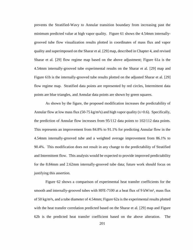
201
prevents the Stratified-Wavy to Annular transition boundary from increasing past the
minimum predicted value at high vapor quality. Figure 61 shows the 4.54mm internally-
grooved tube flow visualization results plotted in coordinates of mass flux and vapor
quality and superimposed on the Sharar et al. [29] map, described in Chapter 4, and revised
Sharar et al. [29] flow regime map based on the above adjustment; Figure 61a is the
4.54mm internally-grooved tube experimental results on the Sharar et al. [29] map and
Figure 61b is the internally-grooved tube results plotted on the adjusted Sharar et al. [29]
flow regime map. Stratified data points are represented by red circles, Intermittent data
points are blue triangles, and Annular data points are shown by green squares.
As shown by the figure, the proposed modification increases the predictability of
Annular flow at low mass flux (50-75 kg/m²s) and high vapor quality (x>0.6). Specifically,
the prediction of Annular flow increases from 95/112 data points to 102/112 data points.
This represents an improvement from 84.8% to 91.1% for predicting Annular flow in the
4.54mm internally-grooved tube and a weighted average improvement from 86.1% to
90.4%. This modification does not result in any change to the predictability of Stratified
and Intermittent flow. This analysis would be expected to provide improved predictability
for the 8.84mm and 2.62mm internally-grooved tube data; future work should focus on
justifying this assertion.
Figure 62 shows a comparison of experimental heat transfer coefficients for the
smooth and internally-grooved tubes with HFE-7100 at a heat flux of 9 kW/m², mass flux
of 50 kg/m²s, and a tube diameter of 4.54mm; Figure 62a is the experimental results plotted
with the heat transfer correlation predicted based on the Sharar et al. [29] map and Figure
62b is the predicted heat transfer coefficient based on the above alteration. The
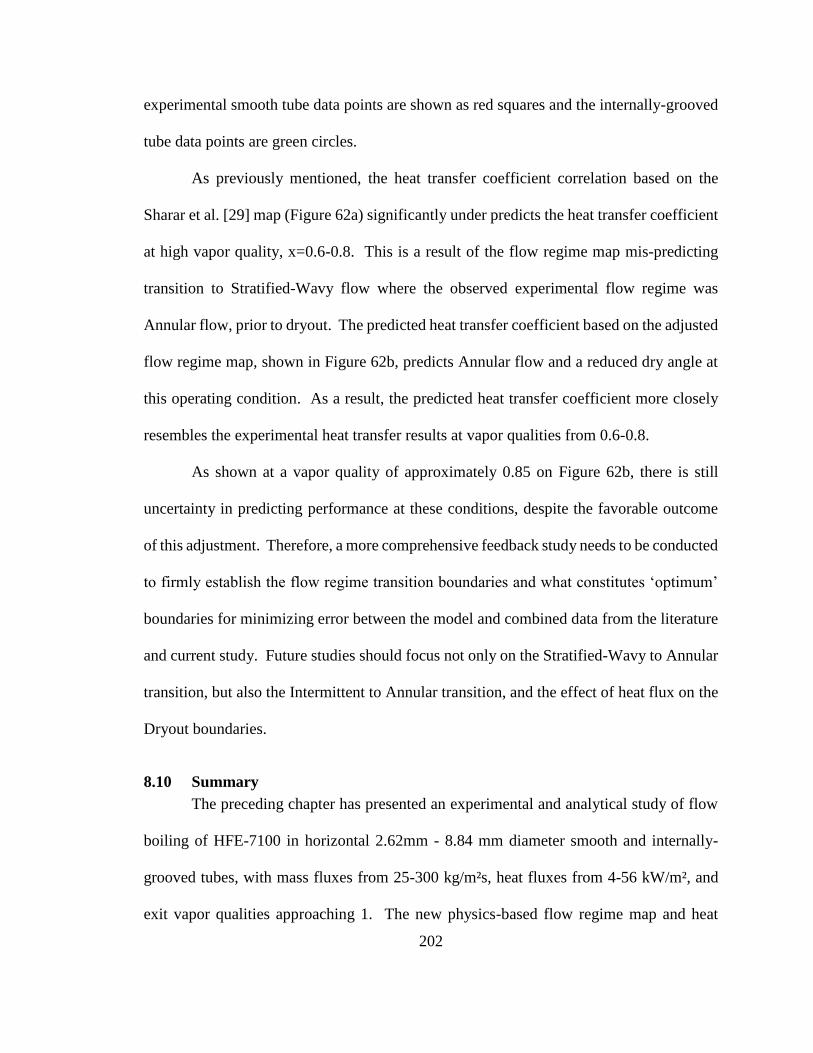
202
experimental smooth tube data points are shown as red squares and the internally-grooved
tube data points are green circles.
As previously mentioned, the heat transfer coefficient correlation based on the
Sharar et al. [29] map (Figure 62a) significantly under predicts the heat transfer coefficient
at high vapor quality, x=0.6-0.8. This is a result of the flow regime map mis-predicting
transition to Stratified-Wavy flow where the observed experimental flow regime was
Annular flow, prior to dryout. The predicted heat transfer coefficient based on the adjusted
flow regime map, shown in Figure 62b, predicts Annular flow and a reduced dry angle at
this operating condition. As a result, the predicted heat transfer coefficient more closely
resembles the experimental heat transfer results at vapor qualities from 0.6-0.8.
As shown at a vapor quality of approximately 0.85 on Figure 62b, there is still
uncertainty in predicting performance at these conditions, despite the favorable outcome
of this adjustment. Therefore, a more comprehensive feedback study needs to be conducted
to firmly establish the flow regime transition boundaries and what constitutes ‘optimum’
boundaries for minimizing error between the model and combined data from the literature
and current study. Future studies should focus not only on the Stratified-Wavy to Annular
transition, but also the Intermittent to Annular transition, and the effect of heat flux on the
Dryout boundaries.
8.10 Summary
The preceding chapter has presented an experimental and analytical study of flow
boiling of HFE-7100 in horizontal 2.62mm - 8.84 mm diameter smooth and internally-
grooved tubes, with mass fluxes from 25-300 kg/m²s, heat fluxes from 4-56 kW/m², and
exit vapor qualities approaching 1. The new physics-based flow regime map and heat

203
transfer model described in Chapter 4 were quantitatively and statistically validated using
the current data and data from the literature. Models from the literature were also compared
to the current data set.
It was shown that the Wojtan et al. [31] regime-based heat transfer coefficient
correlation, with a mean and absolute deviation of -14.0% and 26.9%, outperformed the
smooth tube models of Chen [56], Shah [57], Kandlikar [93], Gungor and Winterton [59],
and simplified two-phase flow boiling correlation by Gungor and Winterton [60]. This
was especially true at mass fluxes below 150 kg/m²s where Stratified-Wavy and Stratified
flow occupied a large portion of the parametric space. Deficiencies in the Wojtan et al.
[31] model for predicting heat transfer coefficient at high heat flux and near dryout
conditions represent a future research opportunity.
Similarly, the new Sharar et al. [29] flow regime map and associated regime-based
heat transfer coefficient correlation outperformed the internally-grooved tube correlations
from Thome et al. [91], Cavallini et al. [117], Chamra and Mago [162], Wu et al. [103],
and Yun et al. [90], particularly at mass fluxes below 75 kg/m²s where Stratified-Wavy and
Stratified flow occupied a large portion of the parametric space; the mean and absolute
deviation for the new model was 4.0% and 32%, respectively. The largest source of
deviation was at high vapor quality where the model predicted dryout and Annular flow
was sustained in the internally-grooved tubes. Additionally, larger-than-normal errors
arose near the transition boundary between Stratified-Wavy and Annular flow, presumably
due to uncertainty in the reported mass flux. Suggestions for future flow regime and heat
transfer model improvements (as well as improvements to the experimental test setup) were
made, focusing primarily on the need for future research on high heat flux, dry-out

204
conditions, and operation close to flow regime transition boundaries. Along these lines, a
section of this chapter was devoted to identifying the merits of altering the newly developed
flow regime map and heat transfer coefficient correlation. This analysis indicated that a
more comprehensive feedback study needs to be conducted to firmly establish the flow
regime transition boundaries and what constitutes ‘optimum’ boundaries for minimizing
error between the model and combined data from the literature and current study.
Based on results from the current study and those from independent researchers, it
was shown that heat transfer enhancement at low-to-intermediate mass flux is primarily
due to early flow regime transition in internally-grooved tubes. Additionally, it was shown
that heat transfer enhancement approaches the area enhancement when the smooth and
internally-grooved tubes are operating in the same flow regime. This applied at sufficiently
low mass flux, where Stratified flow is expected, as well as high mass flux, where Annular
flow is expected. This result fulfills the goal of developing and validating a physics-based
heat transfer model that represents the impact of two-phase flow structures and is coupled
to a reliable flow regime map [105].

205
Chapter 9: Conclusions and Future Work
9.1 Conclusions
The predictive accuracy for two-phase flow boiling in smooth channels has
benefitted from the adoption and proliferation of regime-based heat transfer coefficients.
Unfortunately, the same level of phenomenological insight and physical modeling for
internally-grooved tubes has not yet been developed. Therefore, a stronger experimental
and theoretical knowledge base needs to be established for enhancement in internally-
grooved tubes, focusing on a more comprehensive understanding of the physical
mechanisms responsible for improved performance in these tubes. Pursuant to this goal,
this work focused on the analytical development and experimental validation of a physics-
based flow regime map and heat transfer coefficient model that recognize the role played
by two-phase flow structures in enhancing thermal transport within internally-grooved
tubes.
A detailed analysis of smooth and internally-grooved tube data for two-phase flow
of refrigerants, obtained from the literature and superimposed on the Wojtan et al. [30]
flow regime map, revealed that performance improvement (3-7 times that of a plain tube)
in internally-grooved tubes at low-to-intermediate mass flux is a result of early transition
to Annular flow. At high mass flux where the smooth tube and internally-grooved tube are
operating in Annular flow, the enhancement reduces to the internal area ratio (1.5 to 1.8
times that of a plain tube). The current state of two-phase flow regime maps and heat
transfer correlations for internally-grooved tubes was summarized and motivation for the
current research effort was established.
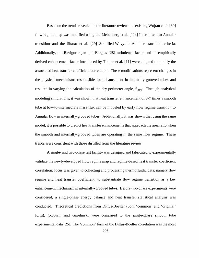
206
Based on the trends revealed in the literature review, the existing Wojtan et al. [30]
flow regime map was modified using the Liebenberg et al. [114] Intermittent to Annular
transition and the Sharar et al. [29] Stratified-Wavy to Annular transition criteria.
Additionally, the Ravigururajan and Bergles [28] turbulence factor and an empirically
derived enhancement factor introduced by Thome et al. [11] were adopted to modify the
associated heat transfer coefficient correlation. These modifications represent changes in
the physical mechanisms responsible for enhancement in internally-grooved tubes and
resulted in varying the calculation of the dry perimeter angle, θdry. Through analytical
modeling simulations, it was shown that heat transfer enhancement of 3-7 times a smooth
tube at low-to-intermediate mass flux can be modeled by early flow regime transition to
Annular flow in internally-grooved tubes. Additionally, it was shown that using the same
model, it is possible to predict heat transfer enhancements that approach the area ratio when
the smooth and internally-grooved tubes are operating in the same flow regime. These
trends were consistent with those distilled from the literature review.
A single- and two-phase test facility was designed and fabricated to experimentally
validate the newly-developed flow regime map and regime-based heat transfer coefficient
correlation; focus was given to collecting and processing thermofluidic data, namely flow
regime and heat transfer coefficient, to substantiate flow regime transition as a key
enhancement mechanism in internally-grooved tubes. Before two-phase experiments were
considered, a single-phase energy balance and heat transfer statistical analysis was
conducted. Theoretical predictions from Dittus-Boelter (both ‘common’ and ‘original’
form), Colburn, and Gnielinski were compared to the single-phase smooth tube
experimental data [25]. The ‘common’ form of the Dittus-Boelter correlation was the most

207
accurate for predicting single-phase flow of HFE-7100 in 2.8mm, 4.54mm, and 8.84mm
smooth tubes with a mean and absolute deviation of 7.07% and 9.02%, respectively. The
Dittus-Boelter (both ‘common’ and ‘original’ form), Colburn, and Gnielinski correlations
were modified using the Ravigururajan and Bergles [28] turbulence factor to predict single-
phase flow in the internally-grooved tubes. The ‘common’ form of the Dittus-Boelter
correlation (modified with the turbulence factor) was the most accurate for predicting
single-phase flow of HFE-7100 in 2.62mm, 4.54mm, and 8.84mm internally-grooved tubes
with a mean and absolute deviation of 4.46% and 11.08%, respectively. This illustrated
that the test setup was functioning properly and the experimental method was robust and
capable of providing reliable measurements. This also validated the use of the
Ravigururajan and Bergles [28] turbulence factor in the heat transfer coefficient correlation
described in this dissertation.
A non-intrusive optical sensor, based on Total Internal Reflection (TIR) and
capable of determining the liquid film thickness, was developed to study the dynamic
nature of two-phase flows. The new method represents a more reliable method for
experimentally determining flow regime compared to the common visual and verbal flow
regime definitions. The method consisted of shining a red fiber-optic light source through
the top of an optically transparent glass tube, using a CMOS camera to capture light rings
resulting from total internal reflection at the liquid-vapor interface, and extracting a film
thickness profile from the resulting images. It was found that different flow regimes
resulted in unique temporally varying film thickness profiles, which were confirmed using
high speed visualization. Using these profiles, quantitative flow regime identification
measures were developed, including the ability to explain and quantify the more subtle

208
transitions that occur between dominant flow regimes. The flow regime maps of Taitel-
Dukler [46], Ullmann-Brauner [141], and Wojtan et al. [30] were found to correlate the
smooth-tube experimental data accurately, to varying degrees, thus validating the use of
the TIR technique in predicting flow regime.
Flow regime data, based on the newly-developed Total Internal Reflection method,
and heat transfer coefficient data, using infrared thermography, was collected for two-
phase HFE-7100 flow in horizontal 2.62mm - 8.84mm diameter smooth and internally-
grooved tubes with mass fluxes from 25-300 kg/m²s, heat fluxes from 4-56 kW/m², and
vapor qualities approaching 1. In total, over 6,500 combined data points for the adiabatic
and diabatic smooth and internally-grooved tubes were acquired.
For the current smooth tube data, it was shown that the Wojtan et al. [31] regime-
based heat transfer coefficient correlation, with a mean and absolute deviation of -14.0%
and 26.9%, outperformed the smooth tube models of Chen [56], Shah [57], Kandlikar [93],
Gungor and Winterton [59], and the simplified two-phase flow boiling correlation by
Gungor and Winterton [60]. This was especially true at mass fluxes below 150 kg/m²s,
where Stratified-Wavy and Stratified flow occupied a large portion of the parametric space.
Similarly, the modified Sharar et al. [29] flow regime map and associated regime-based
heat transfer coefficient correlation, described herein, outperformed the internally-grooved
tube correlations from Thome et al. [91], Cavallini et al. [117], Chamra and Mago [162],
Wu et al. [103], and Yun et al. [90], particularly at mass fluxes below 75 kg/m²s where
Stratified-Wavy and Stratified flow occupied a large portion of the parametric space; the
mean and absolute deviations for the new model were 4.0% and 32%, respectively.
Adoption of the new flow regime map [29] improved flow regime predictive accuracy from

209
66.7% to 88.3% for the current data set and from 65% to 86% when compared to data from
Yu et al. [66], Colombo et al. [79], and Spindler and Müller-Steinhagen [74].
Based on results from the current study and those from independent researchers, it
was shown that heat transfer enhancement at low-to-intermediate mass flux is primarily
due to early flow regime transition in internally-grooved tubes. Additionally, it was shown
that heat transfer enhancement approaches the area enhancement when the smooth and
internally-grooved tubes are operating in the same flow regime. This applied at sufficiently
low mass flux, where Stratified flow is expected, as well as high mass flux, where Annular
flow is expected. These results fulfill the goal of developing a physics-based heat transfer
model that represents the impact of two-phase flow structures in internally-grooved tubes.
9.2 Future Work
Several recommendations for future internally-grooved tube research have been
identified based on the preceding literature review and experimental work:
a. The largest deviation between the current model and experimental results was
at high vapor quality where the model predicted dryout and Annular flow was
sustained in the internally-grooved tubes. Additionally, larger-than-normal
errors arose near the transition boundary between Stratified-Wavy and Annular
flow, presumably due to uncertainty in the reported mass flux. Future research
on high heat flux, dry-out conditions, and operation close to flow regime
transition boundaries should be undertaken.
b. Even though the new flow regime map and heat transfer model improves
predictive accuracy, there is still uncertainty in predicting performance under
certain conditions. It was shown that alterations to the map, based on the

210
collection of new data and data from the literature, can improve flow regime
predictability and subsequently, heat transfer predictability. Therefore, a
comprehensive feedback study needs to be conducted to firmly establish the
flow regime transition boundaries and what constitutes optimum boundaries for
minimizing error between the model and available data. Future studies should
focus not only on the Stratified-Wavy to Annular transition, but also the
Intermittent to Annular transition, and the effect of heat flux on the Dryout
boundaries.
c. Similarly, deficiencies in the Wojtan et al. [31] model for predicting heat
transfer coefficient at high heat flux and near dryout conditions represents
future research opportunities.
d. Researchers have observed performance differences for identical test conditions
but variable tube groove parameters. Therefore, a more systematic study of the
effect of fin shape, fin height, number of fins, helix and apex angle, and ratio of
relevant parameters needs to be undertaken to determine the relationship
between these parameters, flow regime, and thermofluid performance, and what
constitutes a geometrically-optimum tube for given operating conditions.
e. It is not entirely clear what impact operation of refrigerants and CO2 at high
reduced pressure has on flow regimes and heat transfer in internally-grooved
tubes. Future studies are needed. Please refer to Chapter 3 for more details.
f. All of the small diameter internally-grooved tube studies in the literature for
refrigerant/oil mixtures used CO2 at 10ºC and polyalkylene glycol (PAG).
211
Thus, there is a need to extend the experimental database to other refrigerant
and oil combinations.
When undertaking the above tasks, effort should be made to adhere to the following
research guidelines:
a. Concurrent heat transfer and quantitative flow regime data should be collected
over a wide range of operating conditions, particularly low mass flux, to
establish the intrinsic relationship between the dominant flow structure and
thermofluid performance in internally-grooved tubes. Additionally,
comparison to existing correlations, flow regime maps, and smooth tube data
as a means to normalize the results should accompany all experiments to
determine the current state of internally-grooved tube predictive methods.
b. The majority of the studies in the literature relied solely on subjective flow
regime data collection, which calls into question the accuracy of the results.
Future studies should focus on objective flow regime determination methods to
obtain more accurate and repeatable results.

212
Appendix A Atomic Layer Deposition Tube Coating Method
As described in Chapter 5, the smooth and internally-grooved tubes were coated
with 8 μm Parylene-C in a Specialty Coating Systems PDS2010 coating tool followed by
12,000 Å of Titanium and 2,000 Å of Platinum in a CHA E-beam evaporator using a
rotating stepper motor assembly. This supplied a robust, conformal, thin film resistor
necessary to experimentally heat the tubes. However, there were alternative heating
methods that were being explored. This Appendix gives a brief description of candidate
heating methods and focuses on an attempt to create thin film heaters with Atomic Layer
Deposition (ALD).
A.1 Candidate Heating Methods
When choosing a heating method it is important that appropriate heat flux levels
can be met for all of the tubes. For a maximum heat flux of 56 kW/m², the 8.84mm,
4.54mm, and 2.62/2.8mm smooth and internally-grooved tubes need to have 210W, 100W,
and 60W of heat applied, respectively. For the 35V, 10A TENMA DC power supply used,
this suggests resistances of 5.83Ω for the 8.84mm tubes, 12.25Ω for the 4.54mm tubes, and
~20.5Ω for the 2.62 and 2.8mm tubes. In addition to staying within these resistance levels,
the chosen method should provide a uniform heat flux and should allow for IR imaging.
One option was to electrically heat the tubes themselves. In the case of the smooth
and internally-grooved copper tubes, the resistance varied from 91µΩ to 500µΩ. With the
35V 10A TENMA DC power supply, these resistances would only provide 0.05W and
0.009W of thermal energy to the smooth and internally-grooved tubes; this is clearly
inadequate given the goal of 210W to 60W. Thinning of the tube walls through chemical

213
etching or machining would likely double the resistance, and power dissipation, but would
not be adequate to reach high heat fluxes. Wieland does not manufacture stainless steel or
other low electrical conductivity material tubes, therefore, direct heating of the tube wall
was not possible. Another option considered was wrapping the tube with a wire or
electrical heater. However, due to the potential variable contact resistance, and associated
non-uniform heat flux, the wire wrapping method is not an appropriate solution.
Additionally, cross flow of hot water in an annulus was considered prohibitively complex,
would likely not provide a uniform heat flux condition, and would not allow IR imaging.
A.2 Atomic Layer Deposition Heating
One alternative to the above methods was to deposit a thin layer of dielectric
material on the outer surface of the tube followed by a thin layer of metal. This method
would provide electrical isolation between the tube and resistor, allow for IR imaging,
virtually eliminate contact resistance, and provide repeatability if ALD (atomic layer
deposition) or other cleanroom tools are employed. Based on these perceived benefits, an
ALD coated thin film heater was considered a preferred method for heating the smooth and
internally-grooved tubes.
ALD is a chemical vapor deposition (CVD) method that (as-advertised) allows
building nanometer thick, pinhole-free, conformal thin films on any 3D shape and
geometry. Proponents of this technology cite further benefits such as excellent adhesion,
self-terminating reactions, precision, and repeatability. Based on these claims, the use of
ALD appeared to be an attractive solution to coating the tubes.
To provide the primary insulating layer, Alumina was chosen because it has a very
high electrical resistivity, good voltage hold-off (10V/nm) [164]), good thermal

214
conductivity (40W/mK), and is relatively inexpensive. Furthermore, Alumina is widely
used in ALD processes and is, therefore, well characterized. Based on the properties of
Alumina, the insulating layer needed to be at least 3.5nm thick to provide the 35V hold-off
necessary for the power supply; for a large safety factor and a more robust film, a final
thickness of 200nm was deposited. To provide the secondary resistor layer, Ruthenium
was chosen based on lab capabilities. The Ruthenium layer should be 100-250 nm to
provide appropriate resistances and allow the appropriate heat fluxes to be applied. Shown
in Table 21 are the physical properties and thicknesses needed for the copper tube, Alumina
layer, and Ruthenium layer.
Table 21: Material properties of interest for ALD coated copper tubes
Material Thermal Conductivity
(W/mK)
Electrical Resistivity
(nΩ-m)
Voltage Hold-off
(V/nm)
Thickness
(nm)
Copper 400 16.8 - -
Alumina 40 - 10 [164] 200
Ruthenium 117 71 - 100-250
A .2.1 ALD Uniformity
One concern is that the Alumina and, more importantly, the Ruthenium layers are
uniform circumferentially and axially along the tube. If the Alumina is not uniform, it may
not provide the required electrical isolation. Furthermore, if the Ruthenium is not uniform,
then the resistance will vary along the tube and a uniform heat flux condition will not be
obtained. It is difficult to measure film thickness on a curved surface such as a tube. In
order to simulate the sides of the tube (top, bottom, left, and right) several 1” silicon wafers
were attached to a custom cantilever fixture and placed in the ALD tool; a schematic of the
setup is shown in Figure 63. The silicon wafers were plated with several microns of
titanium and copper in an evaporator before the ALD process. The purpose of this step

215
was to better simulate adhesion to the copper tubes and also provide a conducting undercoat
so that probes could be used to determine if the Alumina was insulating.
Figure 63: Schematic (side view) of the cantilever test setup made to test material thickness in the
ALD tool
Using a Cambridge NonoTech Fiji ALD tool, the process consisted of a repeating
cycle of trimethylaluminum (TMA) precursor pulse, purge, H2O pulse, and a final purge
for a total of 2000 cycles. The TMA and H2O yield ALD Al2O3. The process had a
deposition rate of approximately 1 angstrom per cycle, resulting in approximately 200nm
of Alumina. Two different Alumina processes were explored: ‘plasma’ Alumina and
‘thermal’ Alumina. Using an ellipsometer to measure film thickness, results showed that
the Plasma process did not vary axially but varied by as much as 14% circumferentially.
The Thermal process did not vary axially and varied by only 4% circumferentially. For
both processes, the Alumina film was insulating. Therefore, the ‘thermal’ Alumina process
was better suited to coat the copper tubes due to the increased uniformity.
A .2.2 Pinhole Defects in ALD
As discussed above, ALD is advertised as a pinhole-free conformal coating,
however, various researchers including Zhang et al. [165] have shown that Alumina ALD
coatings can suffer from pinholes and defects that can degrade film integrity. Pinholes
top
bottom
left
right

216
would represent a void in the insulating layer and a potential avenue for an electrical short
from the resistive layer to the copper tube. Therefore, before coating with Ruthenium,
experiments were conducted to ensure that the Alumina thin films were pinhole free.
In addition to being uniform and transparent, voids in the ALD thin films can be on
the same order as the films themselves, nanometers, which can make detection a formidable
task. Using conventional microscopy techniques can be difficult for void detection.
Instead, the pinhole defect density can be characterized by using a copper electroplating
visualization technique developed by Zhang et al. [165]. Figure 64 is a schematic showing
the formation of a copper metallic bump on a conductive substrate. In the current case, the
initial copper layer used to better simulate adhesion on the copper tubes serves as the
conductive material. When the sample is placed in an electroplating bath and a potential
is applied between the conductive substrate and the solution, copper will deposit in the
pinhole and a copper bump will form. Not surprisingly, electroplating is commonly used
to make metal nanowires and interconnects in nanoporous templates [166]. As shown in
the schematic, the copper bump is larger in size than the pinhole and also opaque which
makes imaging possible with conventional methods.
Figure 64: Schematic showing a copper metallic bump formed at a defect site when electroplating a
conductive substrate in an electrolytic solution of H2SO4 and CuSO4 (adapted from [165])
electroplating
Copper
Alumina
electroplating bath
Silicon Silicon
Copper
Alumina
Copper
b) a)

217
Figure 65 shows SEM images of an Alumina-coated Silicon substrate that was pre-
treated with a titanium-copper coating. The figure on the left is the substrate before the
electroplating process and the figure on the right is after the plating process. In the current
study, the copper electrolyte bath was composed of 15 g/L of Cu and 210 g/L sulfuric acid
[167]. Samples were plated for 20 minutes each. It is clear from the figure that defects are
not readily apparent before electroplating but copper nodules are clearly visible after
electroplating. For several samples tested, the defect density exceeded 50/cm². Defect
densities on this order would provide paths for potential short circuiting of the thin film
resistor to the underlying conductive substrate/tube. It is reasonable to assume that the
electroplating bath had little to no deleterious effect on the Al2O3 film [168].
Figure 65: Comparison between SEM images of 200nm thick Alumina deposited on Cu-coated Si
substrates a) before and b) after electroplating process
To confirm that the defects would eliminate the necessary electrical isolation,
several copper tubes were coated with 200nm Al2O3 and sent to Impreglon [169] to be
coated with Titanium Nitride (TiN). TiN is an extremely hard ceramic material commonly
used to coat machine tools such as drill bits and milling cutters. In addition to the robust
mechanical properties, TiN is also electrically conductive so it is suitable as a resistive
100 μm 100 μm
b) a)
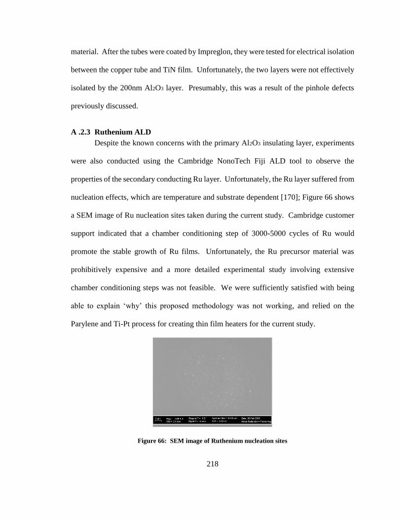
218
material. After the tubes were coated by Impreglon, they were tested for electrical isolation
between the copper tube and TiN film. Unfortunately, the two layers were not effectively
isolated by the 200nm Al2O3 layer. Presumably, this was a result of the pinhole defects
previously discussed.
A .2.3 Ruthenium ALD
Despite the known concerns with the primary Al2O3 insulating layer, experiments
were also conducted using the Cambridge NonoTech Fiji ALD tool to observe the
properties of the secondary conducting Ru layer. Unfortunately, the Ru layer suffered from
nucleation effects, which are temperature and substrate dependent [170]; Figure 66 shows
a SEM image of Ru nucleation sites taken during the current study. Cambridge customer
support indicated that a chamber conditioning step of 3000-5000 cycles of Ru would
promote the stable growth of Ru films. Unfortunately, the Ru precursor material was
prohibitively expensive and a more detailed experimental study involving extensive
chamber conditioning steps was not feasible. We were sufficiently satisfied with being
able to explain ‘why’ this proposed methodology was not working, and relied on the
Parylene and Ti-Pt process for creating thin film heaters for the current study.
Figure 66: SEM image of Ruthenium nucleation sites

219
Appendix B Matlab Code for Total Internal Reflection
This appendix describes the Matlab code used for systematically calculating film
thickness and flow regime for Chapter 6. The process involves pulling the individual ‘.png’
picture files from a specified file location, then undertaking the image processing steps
outlined in Chapter 6 and included below for the reader’s convenience. The basis of the
Matlab algorithm was determining the distance between the light source and the reflected
rays and calculated the liquid film thickness using the following relationship:
tl =x − 2twtanθcwa
2tanθclv
(72)
Several image processing steps were required to extract a film thickness value from
an unrefined image. First, the image was captured with an appropriate camera. Shown in
Figure 67a is a captured image with no film (dry channel). The black shaft on the bottom-
center of the figure is the painted fiber optic LED connecting to the diffuse coating. The
reflected light ring is visible, but not distinct enough to extract accurate film thickness
values. Next, the image was converted to red-only to eliminate background light noise.
Then, adaptive contrast enhancement was performed to normalize the image and remove
complications stemming from intensity variations in the reflected light ring as a result of
LED mounting imperfections. Figure 67b shows the original image after eliminating green
and blue light, and adaptive contrast enhancement. Next, a 2-D median filter was applied
to eliminate salt and pepper noise and a simple contrast enhancement code was applied,
resulting in a binary image, as shown in Figure 67c. The reflected light ring is now clearly
visible.

220
The center of the LED was manually identified. In Figure 67c, the center of the
LED is indicated with a red point. Next, a Sobel filter was used to locate the edges where
the binary image changes from black to white and vice versa; the Sobel filter function
outputs a matrix of these locations. As shown on Figure 67c, the third ‘edge’ identified by
the Sobel filter will represent the first fully reflected ray. Then, a custom Matlab code was
used to count left and right (pixel-by-pixel) out from the LED center point while searching
for the third location where the contrast changes. The diameter of the light ring, in pixels,
is the sum of the distance measured to the left and right. Next, the pixel distance was
translated to a physical distance using the width of the LED (1.27 mm) as a reference scale.
Finally, Equation (49) was used to relate the light ring to a liquid film thickness.
Figure 67: a) Raw image of reflected light ring on a glass tube with no film thickness, b) Image after
converting to black and white and contrast enhancement, and c) Image after converting to binary
The Matlab code used to accomplish this is shown below, along with comments to
assist the reader:
(b) (c)(a)
123
Location of first fully
reflected light ray

221
clc
clear all
close all
B.1 Preprocessing
fiber_dia=0.00127; % diameter of the fiber optic LED
fiber_pix=176; % diameter (in pixels) of the fiber optic
pix=fiber_dia/fiber_pix; % defines m/pixel (pixel ‘length’)
center=[603,360]; % manually determined by inspection
B.2 Importing the Picture and Finding the Location of the First Fully Reflected
Ray
I = imread('183 micrometer calibration.png'); % read the file
figure('Name','I'); % name the figure
imshow(I) % show the figure - Figure 67a
I_2=I(:,:,1); % change the image to red
Max=max(max(I_2)); % find the maximum
Min=min(min(I_2)); % find the minimum
figure('Name','I_2'); % name the figure
imshow(I_2) % show the figure
[N,M]=size(I_2); % size of the 'contrast' matrix

222
filtered=medfilt2(medfilt2(medfilt2(medfilt2(medfilt2(medfilt2((medfilt2(I_2)))))))); %
median filter used to eliminate salt and pepper noise
figure ('Name','filtered'); % name the figure
imshow(filtered) % show the figure
adapthisteq=adapthisteq(filtered,'NumTiles',[8
8],'ClipLimit',0.1,'NBins',1000,'Distribution','uniform'); % adaptive contrast
enhancement based on local maximum and minimum
figure ('Name','adapthisteq'); % name the figure
imshow(adapthisteq) % show the figure
contrast=255*((adapthisteq-Min)/(Max-Min)); % increase the contrast as described by
Shedd and Newell [81]
figure('Name','contrast') % name the figure
imshow(contrast) % show the figure Figure 67b
hold on;
filtered2=medfilt2(medfilt2(medfilt2(medfilt2(medfilt2(medfilt2((medfilt2(contrast,[11
11])))))))); % median filter used to eliminate salt and pepper noise
figure ('Name','filtered2'); % name the figure
imshow(filtered2) % show the figure
hold on
plot(603,360,'r.','MarkerSize',20) % plot the LED center point on the figure

223
sobel=edge(filtered2,'sobel'); % Sobel filter finds the 'edges' of the high contrast region
(highest slope)
figure('Name','sobel'); % name the figure
imshow(sobel) % show the figure
hold on
plot(603,360,'r.','MarkerSize',20) % plot the LED center point on the figure Figure 67c
hold off
B.3 Determining the Number of Pixels Between Lines
iii=0;
jjj=0;
kkk=0;
ring=zeros(N,M);
band=60; % region above and below the center point that will be ‘searched’
% search for first fully reflected ray to the right
for i =center(2)-band/2:center(2)+band/2
iii=0;
jjj=0;
kkk=0;

224
for j =center(1):M
if sobel(i,j) == 1
iii=iii+1 % transition counter
end
if iii == 2
if contrast(i,j) == 0
jjj=jjj+1; % counts number of consecutive black pixels
elseif contrast(i,j) == 255
jjj=0;
end
end
if iii == 3
dist_r(i)=abs(j-center(1));
break
end
end
end
dist_r;

225
% search for first fully reflected ray to the left
i=0;
j=0;
iii=0;
jjj=0;
kkk=0;
for i =center(2)-band/2:center(2)+band/2
iii=0;
jjj=0;
kkk=0;
for jj =center(1):M
kkk=kkk+1;
j=jj-2*kkk; % creating a negatively moving index
if sobel(i,j) == 1
iii=iii+1; % transition counter
end
if iii == 2
if contrast(i,j) == 0
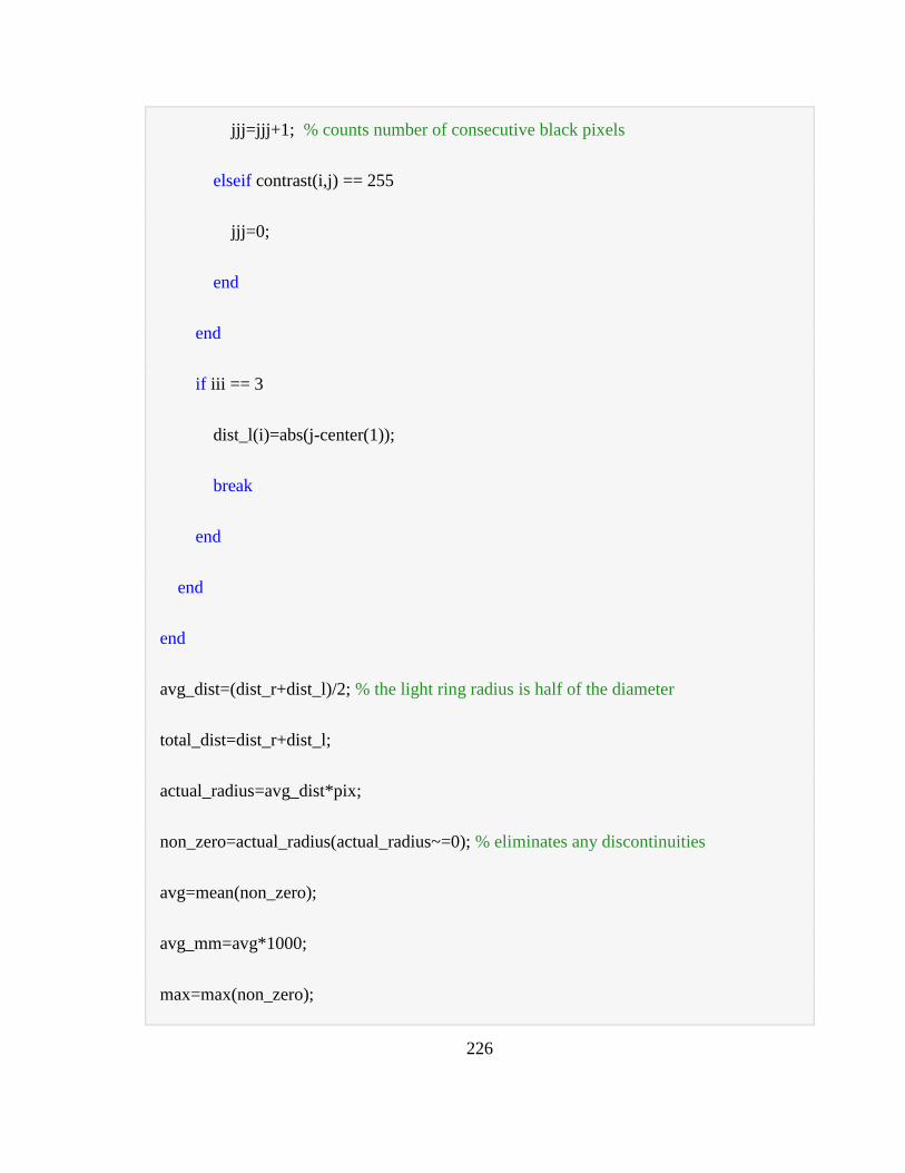
226
jjj=jjj+1; % counts number of consecutive black pixels
elseif contrast(i,j) == 255
jjj=0;
end
end
if iii == 3
dist_l(i)=abs(j-center(1));
break
end
end
end
avg_dist=(dist_r+dist_l)/2; % the light ring radius is half of the diameter
total_dist=dist_r+dist_l;
actual_radius=avg_dist*pix;
non_zero=actual_radius(actual_radius~=0); % eliminates any discontinuities
avg=mean(non_zero);
avg_mm=avg*1000;
max=max(non_zero);

227
max_mm=max*1000;
plot(1:length(avg_dist),avg_dist) % plot the average distance (in pixels)
B.4 Defining Properties and Dimensions
n_tube=1.52; % index of refraction of tube wall (microscope slide)
n_vapor=1; % index of refraction of air/vapor
n_film=1.524; % index of refraction of UV curing adhesive (in actual applications
it will be the index of the fluid at the appropriate temperature)
t_tube=0.00101; % thickness of the tube wall in meters (microscope slide)
avg_dist=avg; % average radius of the light ring in meters
B.5 TIR Film Thickness Calculation
theta_crit_cl=asin(n_vapor/n_film);
theta_crit_cw=asin(n_vapor/n_tube);
theta_crit_wl=asin(n_film/n_tube);
x_dry=2000*t_tube*tan(theta_crit_cw)
thickness_avg=(avg-2*t_tube*tan(theta_crit_cw))/(2*tan(theta_crit_cl))
thickness_mm_avg=thickness_avg*1000
max_thickness=(t_tube*(tan(theta_crit_wl)-tan(theta_crit_cw)))/(tan(theta_crit_cl));

228
x_dry =
1.7646
Thickness_avg =
1.8031e-04
thickness_mm_avg =
0.1803
Published with MATLAB® 7.14

229
Appendix C 8.84mm Smooth and Internally-Grooved Tube
Data
This Appendix is a compilation of all of the diabatic 8.84mm smooth and internally-
grooved tube data collected during the course of this study; in total, 2098 diabatic data
points are shown below. The Wojtan et al. [31] heat transfer coefficient correlation as well
as the correlation developed in this dissertation are included for reference. Select figures
from this data set were used for the analysis in Chapter 8. Please refer to Chapter 8 for a
description of the more salient trends observed; this Appendix mainly serves as a means to
document the entirety of the experimental results.
Each figure represents a different flowrate (25-300 kg/m²s) and six different heat
fluxes (4-56 kW/m²s). In some scenarios, high heat fluxes could not be accurately
measured because the heat transfer coefficient was too low or dryout occurred and the tube
overheated. However, the heat transfer coefficient correlations were still included for
reference. One example of this is Figure 75 with a heat flux of 56 kW/m²s.
The experimental smooth tube data points are shown as red squares and the
internally-grooved tube data points are green circles. ‘IG 1’ and ‘smooth 1’ were the first
tests run and ‘IG 2’ and ‘smooth 2’ were the second tests run; as indicated in Chapter 8,
these do not represent different tubes, just a second run of experiments for validation. The
smooth tube heat transfer coefficient correlation [31] and the current internally-grooved
tube heat transfer coefficient correlation are plotted as solid red and dashed green lines,
respectively.

230
Figure 68: Heat transfer coefficient vs vapor quality for 8.84 mm ID smooth and internally-grooved
tubes at a mass flux of 300 kg/m²s and different heat fluxes
0
1000
2000
3000
4000
5000
6000
7000
8000
9000
10000
11000
12000
13000
0.0 0.1 0.2 0.3 0.4 0.5 0.6 0.7 0.8 0.9 1.0
Hea
t T
ransf
er C
oef
fici
ent
(W/m
²K)
x
0
1000
2000
3000
4000
5000
6000
7000
8000
9000
10000
11000
0.0 0.1 0.2 0.3 0.4 0.5 0.6 0.7 0.8 0.9 1.0
Hea
t T
ransf
er C
oef
fici
ent
(W/m
²K)
x
0
1000
2000
3000
4000
5000
6000
7000
8000
9000
10000
0.0 0.1 0.2 0.3 0.4 0.5 0.6 0.7 0.8 0.9 1.0
Hea
t T
ransf
er C
oef
fici
ent
(W/m
²K)
x
0
1000
2000
3000
4000
5000
6000
7000
8000
9000
0.0 0.1 0.2 0.3 0.4 0.5 0.6 0.7 0.8 0.9 1.0
Hea
t T
ransf
er C
oef
fici
ent
(W/m
²K)
x
0
1000
2000
3000
4000
5000
6000
7000
8000
9000
0.0 0.1 0.2 0.3 0.4 0.5 0.6 0.7 0.8 0.9 1.0
Hea
t T
ransf
er C
oef
fici
ent
(W/m
²K)
x
0
1000
2000
3000
4000
5000
6000
7000
8000
9000
0.0 0.1 0.2 0.3 0.4 0.5 0.6 0.7 0.8 0.9 1.0
Hea
t T
ransf
er C
oef
fici
ent
(W/m
²K)
x0
100020003000400050006000700080009000
10000110001200013000140001500016000170001800019000
0.0 0.1 0.2 0.3 0.4 0.5 0.6 0.7 0.8 0.9 1.0
Current Wojtan IG 1 IG 2 smooth 1 smooth 2
4 kW/m² 9 kW/m²
18 kW/m² 28 kW/m²
40 kW/m² 56 kW/m²
Modified

231
Figure 69: Heat transfer coefficient vs vapor quality for 8.84 mm ID smooth and internally-grooved
tubes at a mass flux of 200 kg/m²s and different heat fluxes
0
1000
2000
3000
4000
5000
6000
7000
8000
9000
10000
11000
12000
0.0 0.1 0.2 0.3 0.4 0.5 0.6 0.7 0.8 0.9 1.0
Hea
t T
ransf
er C
oef
fici
ent
(W/m
²K)
x
0
1000
2000
3000
4000
5000
6000
7000
8000
9000
10000
11000
0.0 0.1 0.2 0.3 0.4 0.5 0.6 0.7 0.8 0.9 1.0
Hea
t T
ransf
er C
oef
fici
ent
(W/m
²K)
x
0
1000
2000
3000
4000
5000
6000
7000
8000
9000
10000
11000
0.0 0.1 0.2 0.3 0.4 0.5 0.6 0.7 0.8 0.9 1.0
Hea
t T
ransf
er C
oef
fici
ent
(W/m
²K)
x
0
1000
2000
3000
4000
5000
6000
7000
8000
9000
10000
0.0 0.1 0.2 0.3 0.4 0.5 0.6 0.7 0.8 0.9 1.0
Hea
t T
ransf
er C
oef
fici
ent
(W/m
²K)
x
0
1000
2000
3000
4000
5000
6000
7000
8000
9000
10000
0.0 0.1 0.2 0.3 0.4 0.5 0.6 0.7 0.8 0.9 1.0
Hea
t T
ransf
er C
oef
fici
ent
(W/m
²K)
x
0
1000
2000
3000
4000
5000
6000
7000
8000
9000
0.0 0.1 0.2 0.3 0.4 0.5 0.6 0.7 0.8 0.9 1.0
Hea
t T
ransf
er C
oef
fici
ent
(W/m
²K)
x0
100020003000400050006000700080009000
10000110001200013000140001500016000170001800019000
0.0 0.1 0.2 0.3 0.4 0.5 0.6 0.7 0.8 0.9 1.0
Current Wojtan IG 1 IG 2 smooth 1 smooth 2
4 kW/m² 9 kW/m²
18 kW/m² 28 kW/m²
40 kW/m² 56 kW/m²
Modified

232
Figure 70: Heat transfer coefficient vs vapor quality for 8.84 mm ID smooth and internally-grooved
tubes at a mass flux of 175 kg/m²s and different heat fluxes
0
1000
2000
3000
4000
5000
6000
7000
8000
9000
10000
11000
12000
0.0 0.1 0.2 0.3 0.4 0.5 0.6 0.7 0.8 0.9 1.0
Hea
t T
ransf
er C
oef
fici
ent
(W/m
²K)
x
0
1000
2000
3000
4000
5000
6000
7000
8000
9000
10000
11000
0.0 0.1 0.2 0.3 0.4 0.5 0.6 0.7 0.8 0.9 1.0
Hea
t T
ransf
er C
oef
fici
ent
(W/m
²K)
x
0100020003000400050006000700080009000
1000011000120001300014000
0.0 0.1 0.2 0.3 0.4 0.5 0.6 0.7 0.8 0.9 1.0
Hea
t T
ransf
er C
oef
fici
ent
(W/m
²K)
x
0
1000
2000
3000
4000
5000
6000
7000
8000
9000
10000
11000
0.0 0.1 0.2 0.3 0.4 0.5 0.6 0.7 0.8 0.9 1.0
Hea
t T
ransf
er C
oef
fici
ent
(W/m
²K)
x
0
1000
2000
3000
4000
5000
6000
7000
8000
9000
10000
0.0 0.1 0.2 0.3 0.4 0.5 0.6 0.7 0.8 0.9 1.0
Hea
t T
ransf
er C
oef
fici
ent
(W/m
²K)
x
0
1000
2000
3000
4000
5000
6000
7000
8000
9000
0.0 0.1 0.2 0.3 0.4 0.5 0.6 0.7 0.8 0.9 1.0
Hea
t T
ransf
er C
oef
fici
ent
(W/m
²K)
x0
100020003000400050006000700080009000
10000110001200013000140001500016000170001800019000
0.0 0.1 0.2 0.3 0.4 0.5 0.6 0.7 0.8 0.9 1.0
Current Wojtan IG 1 IG 2 smooth 1 smooth 2
4 kW/m² 9 kW/m²
18 kW/m² 28 kW/m²
40 kW/m² 56 kW/m²
Modified
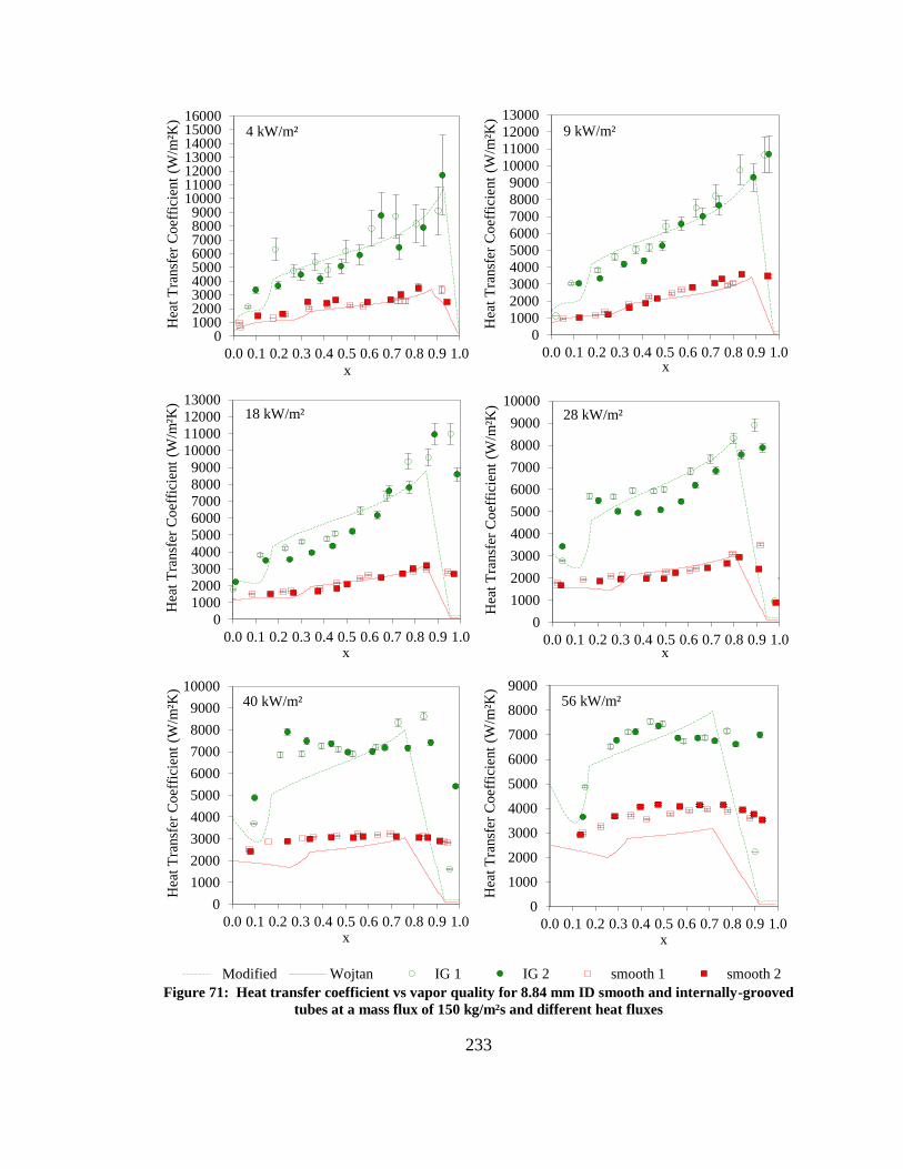
233
Figure 71: Heat transfer coefficient vs vapor quality for 8.84 mm ID smooth and internally-grooved
tubes at a mass flux of 150 kg/m²s and different heat fluxes
0100020003000400050006000700080009000
10000110001200013000140001500016000
0.0 0.1 0.2 0.3 0.4 0.5 0.6 0.7 0.8 0.9 1.0
Hea
t T
ransf
er C
oef
fici
ent
(W/m
²K)
x
0
1000
2000
3000
4000
5000
6000
7000
8000
9000
10000
11000
12000
13000
0.0 0.1 0.2 0.3 0.4 0.5 0.6 0.7 0.8 0.9 1.0
Hea
t T
ransf
er C
oef
fici
ent
(W/m
²K)
x
0
1000
2000
3000
4000
5000
6000
7000
8000
9000
10000
11000
12000
13000
0.0 0.1 0.2 0.3 0.4 0.5 0.6 0.7 0.8 0.9 1.0
Hea
t T
ransf
er C
oef
fici
ent
(W/m
²K)
x
0
1000
2000
3000
4000
5000
6000
7000
8000
9000
10000
0.0 0.1 0.2 0.3 0.4 0.5 0.6 0.7 0.8 0.9 1.0
Hea
t T
ransf
er C
oef
fici
ent
(W/m
²K)
x
0
1000
2000
3000
4000
5000
6000
7000
8000
9000
10000
0.0 0.1 0.2 0.3 0.4 0.5 0.6 0.7 0.8 0.9 1.0
Hea
t T
ransf
er C
oef
fici
ent
(W/m
²K)
x
0
1000
2000
3000
4000
5000
6000
7000
8000
9000
0.0 0.1 0.2 0.3 0.4 0.5 0.6 0.7 0.8 0.9 1.0
Hea
t T
ransf
er C
oef
fici
ent
(W/m
²K)
x0
100020003000400050006000700080009000
10000110001200013000140001500016000170001800019000
0.0 0.1 0.2 0.3 0.4 0.5 0.6 0.7 0.8 0.9 1.0
Current Wojtan IG 1 IG 2 smooth 1 smooth 2
4 kW/m² 9 kW/m²
18 kW/m² 28 kW/m²
40 kW/m² 56 kW/m²
Modified

234
Figure 72: Heat transfer coefficient vs vapor quality for 8.84 mm ID smooth and internally-grooved
tubes at a mass flux of 125 kg/m²s and different heat fluxes
0100020003000400050006000700080009000
1000011000120001300014000
0.0 0.1 0.2 0.3 0.4 0.5 0.6 0.7 0.8 0.9 1.0
Hea
t T
ransf
er C
oef
fici
ent
(W/m
²K)
x
0
1000
2000
3000
4000
5000
6000
7000
8000
9000
10000
11000
12000
0.0 0.1 0.2 0.3 0.4 0.5 0.6 0.7 0.8 0.9 1.0
Hea
t T
ransf
er C
oef
fici
ent
(W/m
²K)
x
0
1000
2000
3000
4000
5000
6000
7000
8000
9000
10000
0.0 0.1 0.2 0.3 0.4 0.5 0.6 0.7 0.8 0.9 1.0
Hea
t T
ransf
er C
oef
fici
ent
(W/m
²K)
x
0
1000
2000
3000
4000
5000
6000
7000
8000
9000
0.0 0.1 0.2 0.3 0.4 0.5 0.6 0.7 0.8 0.9 1.0
Hea
t T
ransf
er C
oef
fici
ent
(W/m
²K)
x
0
1000
2000
3000
4000
5000
6000
7000
8000
9000
10000
0.0 0.1 0.2 0.3 0.4 0.5 0.6 0.7 0.8 0.9 1.0
Hea
t T
ransf
er C
oef
fici
ent
(W/m
²K)
x
0
1000
2000
3000
4000
5000
6000
7000
8000
9000
0.0 0.1 0.2 0.3 0.4 0.5 0.6 0.7 0.8 0.9 1.0
Hea
t T
ransf
er C
oef
fici
ent
(W/m
²K)
x0
100020003000400050006000700080009000
10000110001200013000140001500016000170001800019000
0.0 0.1 0.2 0.3 0.4 0.5 0.6 0.7 0.8 0.9 1.0
Current Wojtan IG 1 IG 2 smooth 1 smooth 2
4 kW/m² 9 kW/m²
18 kW/m² 28 kW/m²
40 kW/m² 56 kW/m²
Modified

235
Figure 73: Heat transfer coefficient vs vapor quality for 8.84 mm ID smooth and internally-grooved
tubes at a mass flux of 100 kg/m²s and different heat fluxes
0
1000
2000
3000
4000
5000
6000
7000
8000
9000
10000
0.0 0.1 0.2 0.3 0.4 0.5 0.6 0.7 0.8 0.9 1.0
Hea
t T
ransf
er C
oef
fici
ent
(W/m
²K)
x
0
1000
2000
3000
4000
5000
6000
7000
8000
9000
0.0 0.1 0.2 0.3 0.4 0.5 0.6 0.7 0.8 0.9 1.0
Hea
t T
ransf
er C
oef
fici
ent
(W/m
²K)
x
0
1000
2000
3000
4000
5000
6000
7000
8000
9000
0.0 0.1 0.2 0.3 0.4 0.5 0.6 0.7 0.8 0.9 1.0
Hea
t T
ransf
er C
oef
fici
ent
(W/m
²K)
x
0
1000
2000
3000
4000
5000
6000
7000
8000
0.0 0.1 0.2 0.3 0.4 0.5 0.6 0.7 0.8 0.9 1.0
Hea
t T
ransf
er C
oef
fici
ent
(W/m
²K)
x
0
1000
2000
3000
4000
5000
6000
7000
8000
9000
0.0 0.1 0.2 0.3 0.4 0.5 0.6 0.7 0.8 0.9 1.0
Hea
t T
ransf
er C
oef
fici
ent
(W/m
²K)
x
0
1000
2000
3000
4000
5000
6000
7000
8000
9000
10000
0.0 0.1 0.2 0.3 0.4 0.5 0.6 0.7 0.8 0.9 1.0
Hea
t T
ransf
er C
oef
fici
ent
(W/m
²K)
x0
100020003000400050006000700080009000
10000110001200013000140001500016000170001800019000
0.0 0.1 0.2 0.3 0.4 0.5 0.6 0.7 0.8 0.9 1.0
Current Wojtan IG 1 IG 2 smooth 1 smooth 2
4 kW/m² 9 kW/m²
18 kW/m² 28 kW/m²
40 kW/m² 56 kW/m²
Modified

236
Figure 74: Heat transfer coefficient vs vapor quality for 8.84 mm ID smooth and internally-grooved
tubes at a mass flux of 75 kg/m²s and different heat fluxes
0
1000
2000
3000
4000
5000
6000
7000
8000
9000
0.0 0.1 0.2 0.3 0.4 0.5 0.6 0.7 0.8 0.9 1.0
Hea
t T
ransf
er C
oef
fici
ent
(W/m
²K)
x
0
1000
2000
3000
4000
5000
6000
7000
8000
9000
0.0 0.1 0.2 0.3 0.4 0.5 0.6 0.7 0.8 0.9 1.0
Hea
t T
ransf
er C
oef
fici
ent
(W/m
²K)
x
0
1000
2000
3000
4000
5000
6000
7000
0.0 0.1 0.2 0.3 0.4 0.5 0.6 0.7 0.8 0.9 1.0
Hea
t T
ransf
er C
oef
fici
ent
(W/m
²K)
x
0
1000
2000
3000
4000
5000
6000
7000
0.0 0.1 0.2 0.3 0.4 0.5 0.6 0.7 0.8 0.9 1.0
Hea
t T
ransf
er C
oef
fici
ent
(W/m
²K)
x
0
1000
2000
3000
4000
5000
6000
7000
8000
0.0 0.1 0.2 0.3 0.4 0.5 0.6 0.7 0.8 0.9 1.0
Hea
t T
ransf
er C
oef
fici
ent
(W/m
²K)
x
0
1000
2000
3000
4000
5000
6000
7000
8000
9000
0.0 0.1 0.2 0.3 0.4 0.5 0.6 0.7 0.8 0.9 1.0
Hea
t T
ransf
er C
oef
fici
ent
(W/m
²K)
x0
100020003000400050006000700080009000
10000110001200013000140001500016000170001800019000
0.0 0.1 0.2 0.3 0.4 0.5 0.6 0.7 0.8 0.9 1.0
Current Wojtan IG 1 IG 2 smooth 1 smooth 2
4 kW/m² 9 kW/m²
18 kW/m² 28 kW/m²
40 kW/m² 56 kW/m²
Modified

237
Figure 75: Heat transfer coefficient vs vapor quality for 8.84 mm ID smooth and internally-grooved
tubes at a mass flux of 50 kg/m²s and different heat fluxes
0
1000
2000
3000
4000
5000
0.0 0.1 0.2 0.3 0.4 0.5 0.6 0.7 0.8 0.9 1.0
Hea
t T
ransf
er C
oef
fici
ent
(W/m
²K)
x
0
1000
2000
3000
4000
0.0 0.1 0.2 0.3 0.4 0.5 0.6 0.7 0.8 0.9 1.0
Hea
t T
ransf
er C
oef
fici
ent
(W/m
²K)
x
0
1000
2000
3000
4000
5000
0.0 0.1 0.2 0.3 0.4 0.5 0.6 0.7 0.8 0.9 1.0
Hea
t T
ransf
er C
oef
fici
ent
(W/m
²K)
x
0
1000
2000
3000
4000
5000
0.0 0.1 0.2 0.3 0.4 0.5 0.6 0.7 0.8 0.9 1.0
Hea
t T
ransf
er C
oef
fici
ent
(W/m
²K)
x
0
1000
2000
3000
4000
5000
0.0 0.1 0.2 0.3 0.4 0.5 0.6 0.7 0.8 0.9 1.0
Hea
t T
ransf
er C
oef
fici
ent
(W/m
²K)
x
0
1000
2000
3000
4000
5000
0.0 0.1 0.2 0.3 0.4 0.5 0.6 0.7 0.8 0.9 1.0
Hea
t T
ransf
er C
oef
fici
ent
(W/m
²K)
x0
100020003000400050006000700080009000
10000110001200013000140001500016000170001800019000
0.0 0.1 0.2 0.3 0.4 0.5 0.6 0.7 0.8 0.9 1.0
Current Wojtan IG 1 IG 2 smooth 1 smooth 2
4 kW/m² 9 kW/m²
18 kW/m² 28 kW/m²
40 kW/m² 56 kW/m²
Modified

238
Figure 76: Heat transfer coefficient vs vapor quality for 8.84 mm ID smooth and internally-grooved
tubes at a mass flux of 25 kg/m²s and different heat fluxes
0
1000
2000
0.0 0.1 0.2 0.3 0.4 0.5 0.6 0.7 0.8 0.9 1.0
Hea
t T
ransf
er C
oef
fici
ent
(W/m
²K)
x
0
1000
2000
0.0 0.1 0.2 0.3 0.4 0.5 0.6 0.7 0.8 0.9 1.0
Hea
t T
ransf
er C
oef
fici
ent
(W/m
²K)
x
0
1000
2000
0.0 0.1 0.2 0.3 0.4 0.5 0.6 0.7 0.8 0.9 1.0
Hea
t T
ransf
er C
oef
fici
ent
(W/m
²K)
x
0
1000
2000
3000
0.0 0.1 0.2 0.3 0.4 0.5 0.6 0.7 0.8 0.9 1.0
Hea
t T
ransf
er C
oef
fici
ent
(W/m
²K)
x
0
1000
2000
3000
4000
0.0 0.1 0.2 0.3 0.4 0.5 0.6 0.7 0.8 0.9 1.0
Hea
t T
ransf
er C
oef
fici
ent
(W/m
²K)
x
0
1000
2000
3000
4000
0.0 0.1 0.2 0.3 0.4 0.5 0.6 0.7 0.8 0.9 1.0
Hea
t T
ransf
er C
oef
fici
ent
(W/m
²K)
x0
100020003000400050006000700080009000
10000110001200013000140001500016000170001800019000
0.0 0.1 0.2 0.3 0.4 0.5 0.6 0.7 0.8 0.9 1.0
Current Wojtan IG 1 IG 2 smooth 1 smooth 2
4 kW/m² 9 kW/m²
18 kW/m² 28 kW/m²
40 kW/m² 56 kW/m²
Modified

239
Appendix D 4.54mm Smooth and Internally-Grooved Tube
Data
This Appendix is a compilation of all of the diabatic 4.54mm smooth and internally-
grooved tube data collected during the course of this study; in total, 1722 diabatic data
points are shown below. The Wojtan et al. [31] heat transfer coefficient correlation as well
as the correlation developed in this dissertation are included for reference. Select figures
from this data set were used for the analysis in Chapter 8. Please refer to Chapter 8 for a
description of the more salient trends observed; this Appendix mainly serves as a means to
document the entirety of the experimental results.
Each figure represents a different flowrate (50-300 kg/m²s) and six different heat
fluxes (4-56 kW/m²s). In some scenarios, high heat fluxes could not be accurately
measured because the heat transfer coefficient was too low or dryout occurred and the tube
overheated. However, the heat transfer coefficient correlations were still included for
reference. One example of this is Figure 84 with a heat flux of 56 kW/m²s.
The experimental smooth tube data points are shown as red squares and the
internally-grooved tube data points are green circles. ‘IG 1’ and ‘smooth 1’ were the first
tests run and ‘IG 2’ and ‘smooth 2’ were the second tests run; as indicated in Chapter 8,
these do not represent different tubes, just a second run of experiments for validation. The
smooth tube heat transfer coefficient correlation [31] and the current internally-grooved
tube heat transfer coefficient correlation are plotted as solid red and dashed green lines,
respectively.

240
Figure 77: Heat transfer coefficient vs vapor quality for 4.54 mm ID smooth and internally-grooved
tubes at a mass flux of 300 kg/m²s and different heat fluxes
0
2000
4000
6000
8000
10000
12000
14000
16000
0.0 0.1 0.2 0.3 0.4 0.5 0.6 0.7 0.8 0.9 1.0
Hea
t T
ransf
er C
oef
fici
ent
(W/m
²K)
x
0
2000
4000
6000
8000
10000
12000
14000
16000
0.0 0.1 0.2 0.3 0.4 0.5 0.6 0.7 0.8 0.9 1.0
Hea
t T
ransf
er C
oef
fici
ent
(W/m
²K)
x
0
2000
4000
6000
8000
10000
12000
14000
16000
0.0 0.1 0.2 0.3 0.4 0.5 0.6 0.7 0.8 0.9 1.0
Hea
t T
ransf
er C
oef
fici
ent
(W/m
²K)
x
0
2000
4000
6000
8000
10000
12000
14000
16000
0.0 0.1 0.2 0.3 0.4 0.5 0.6 0.7 0.8 0.9 1.0
Hea
t T
ransf
er C
oef
fici
ent
(W/m
²K)
x
0
2000
4000
6000
8000
10000
12000
14000
16000
0.0 0.1 0.2 0.3 0.4 0.5 0.6 0.7 0.8 0.9 1.0
Hea
t T
ransf
er C
oef
fici
ent
(W/m
²K)
x
0
2000
4000
6000
8000
10000
12000
14000
16000
0.0 0.1 0.2 0.3 0.4 0.5 0.6 0.7 0.8 0.9 1.0
Hea
t T
ransf
er C
oef
fici
ent
(W/m
²K)
x0
100020003000400050006000700080009000
10000110001200013000140001500016000170001800019000
0.0 0.1 0.2 0.3 0.4 0.5 0.6 0.7 0.8 0.9 1.0
Current Wojtan IG 1 IG 2 smooth 1 smooth 2
4 kW/m² 9 kW/m²
18 kW/m² 28 kW/m²
40 kW/m² 56 kW/m²
Modified

241
Figure 78: Heat transfer coefficient vs vapor quality for 4.54 mm ID smooth and internally-grooved
tubes at a mass flux of 200 kg/m²s and different heat fluxes
0
2000
4000
6000
8000
10000
12000
14000
16000
0.0 0.1 0.2 0.3 0.4 0.5 0.6 0.7 0.8 0.9 1.0
Hea
t T
ransf
er C
oef
fici
ent
(W/m
²K)
x
0
2000
4000
6000
8000
10000
12000
14000
16000
0.0 0.1 0.2 0.3 0.4 0.5 0.6 0.7 0.8 0.9 1.0
Hea
t T
ransf
er C
oef
fici
ent
(W/m
²K)
x
0
2000
4000
6000
8000
10000
12000
14000
16000
0.0 0.1 0.2 0.3 0.4 0.5 0.6 0.7 0.8 0.9 1.0
Hea
t T
ransf
er C
oef
fici
ent
(W/m
²K)
x
0
2000
4000
6000
8000
10000
12000
14000
0.0 0.1 0.2 0.3 0.4 0.5 0.6 0.7 0.8 0.9 1.0
Hea
t T
ransf
er C
oef
fici
ent
(W/m
²K)
x
0
2000
4000
6000
8000
10000
12000
14000
16000
0.0 0.1 0.2 0.3 0.4 0.5 0.6 0.7 0.8 0.9 1.0
Hea
t T
ransf
er C
oef
fici
ent
(W/m
²K)
x
0
2000
4000
6000
8000
10000
12000
14000
16000
0.0 0.1 0.2 0.3 0.4 0.5 0.6 0.7 0.8 0.9 1.0
Hea
t T
ransf
er C
oef
fici
ent
(W/m
²K)
x0
100020003000400050006000700080009000
10000110001200013000140001500016000170001800019000
0.0 0.1 0.2 0.3 0.4 0.5 0.6 0.7 0.8 0.9 1.0
Current Wojtan IG 1 IG 2 smooth 1 smooth 2
4 kW/m² 9 kW/m²
18 kW/m² 28 kW/m²
40 kW/m² 56 kW/m²
Modified

242
Figure 79: Heat transfer coefficient vs vapor quality for 4.54 mm ID smooth and internally-grooved
tubes at a mass flux of 175 kg/m²s and different heat fluxes
0
5000
10000
15000
20000
25000
0.0 0.1 0.2 0.3 0.4 0.5 0.6 0.7 0.8 0.9 1.0
Hea
t T
ransf
er C
oef
fici
ent
(W/m
²K)
x
0
2000
4000
6000
8000
10000
12000
14000
16000
18000
0.0 0.1 0.2 0.3 0.4 0.5 0.6 0.7 0.8 0.9 1.0
Hea
t T
ransf
er C
oef
fici
ent
(W/m
²K)
x
0
2000
4000
6000
8000
10000
12000
14000
0.0 0.1 0.2 0.3 0.4 0.5 0.6 0.7 0.8 0.9 1.0
Hea
t T
ransf
er C
oef
fici
ent
(W/m
²K)
x
0
2000
4000
6000
8000
10000
12000
14000
16000
18000
0.0 0.1 0.2 0.3 0.4 0.5 0.6 0.7 0.8 0.9 1.0
Hea
t T
ransf
er C
oef
fici
ent
(W/m
²K)
x
0
2000
4000
6000
8000
10000
12000
14000
0.0 0.1 0.2 0.3 0.4 0.5 0.6 0.7 0.8 0.9 1.0
Hea
t T
ransf
er C
oef
fici
ent
(W/m
²K)
x
0
2000
4000
6000
8000
10000
12000
14000
0.0 0.1 0.2 0.3 0.4 0.5 0.6 0.7 0.8 0.9 1.0
Hea
t T
ransf
er C
oef
fici
ent
(W/m
²K)
x0
100020003000400050006000700080009000
10000110001200013000140001500016000170001800019000
0.0 0.1 0.2 0.3 0.4 0.5 0.6 0.7 0.8 0.9 1.0
Current Wojtan IG 1 IG 2 smooth 1 smooth 2
4 kW/m² 9 kW/m²
18 kW/m² 28 kW/m²
40 kW/m² 56 kW/m²
Modified

243
Figure 80: Heat transfer coefficient vs vapor quality for 4.54 mm ID smooth and internally-grooved
tubes at a mass flux of 150 kg/m²s and different heat fluxes
0
2000
4000
6000
8000
10000
12000
14000
16000
0.0 0.1 0.2 0.3 0.4 0.5 0.6 0.7 0.8 0.9 1.0
Hea
t T
ransf
er C
oef
fici
ent
(W/m
²K)
x
0
2000
4000
6000
8000
10000
12000
14000
16000
18000
20000
0.0 0.1 0.2 0.3 0.4 0.5 0.6 0.7 0.8 0.9 1.0
Hea
t T
ransf
er C
oef
fici
ent
(W/m
²K)
x
0
2000
4000
6000
8000
10000
12000
14000
0.0 0.1 0.2 0.3 0.4 0.5 0.6 0.7 0.8 0.9 1.0
Hea
t T
ransf
er C
oef
fici
ent
(W/m
²K)
x
0
2000
4000
6000
8000
10000
12000
14000
0.0 0.1 0.2 0.3 0.4 0.5 0.6 0.7 0.8 0.9 1.0
Hea
t T
ransf
er C
oef
fici
ent
(W/m
²K)
x
0
2000
4000
6000
8000
10000
12000
14000
16000
0.0 0.1 0.2 0.3 0.4 0.5 0.6 0.7 0.8 0.9 1.0
Hea
t T
ransf
er C
oef
fici
ent
(W/m
²K)
x
0
2000
4000
6000
8000
10000
12000
0.0 0.1 0.2 0.3 0.4 0.5 0.6 0.7 0.8 0.9 1.0
Hea
t T
ransf
er C
oef
fici
ent
(W/m
²K)
x0
100020003000400050006000700080009000
10000110001200013000140001500016000170001800019000
0.0 0.1 0.2 0.3 0.4 0.5 0.6 0.7 0.8 0.9 1.0
Current Wojtan IG 1 IG 2 smooth 1 smooth 2
4 kW/m² 9 kW/m²
18 kW/m² 28 kW/m²
40 kW/m² 56 kW/m²
Modified

244
Figure 81: Heat transfer coefficient vs vapor quality for 4.54 mm ID smooth and internally-grooved
tubes at a mass flux of 125 kg/m²s and different heat fluxes
0
2000
4000
6000
8000
10000
12000
0.0 0.1 0.2 0.3 0.4 0.5 0.6 0.7 0.8 0.9 1.0
Hea
t T
ransf
er C
oef
fici
ent
(W/m
²K)
x
0
2000
4000
6000
8000
10000
12000
0.0 0.1 0.2 0.3 0.4 0.5 0.6 0.7 0.8 0.9 1.0
Hea
t T
ransf
er C
oef
fici
ent
(W/m
²K)
x
0
2000
4000
6000
8000
10000
12000
0.0 0.1 0.2 0.3 0.4 0.5 0.6 0.7 0.8 0.9 1.0
Hea
t T
ransf
er C
oef
fici
ent
(W/m
²K)
x
0
2000
4000
6000
8000
10000
12000
0.0 0.1 0.2 0.3 0.4 0.5 0.6 0.7 0.8 0.9 1.0
Hea
t T
ransf
er C
oef
fici
ent
(W/m
²K)
x
0
1000
2000
3000
4000
5000
6000
7000
8000
9000
10000
0.0 0.1 0.2 0.3 0.4 0.5 0.6 0.7 0.8 0.9 1.0
Hea
t T
ransf
er C
oef
fici
ent
(W/m
²K)
x
0
1000
2000
3000
4000
5000
6000
7000
8000
9000
10000
0.0 0.1 0.2 0.3 0.4 0.5 0.6 0.7 0.8 0.9 1.0
Hea
t T
ransf
er C
oef
fici
ent
(W/m
²K)
x0
100020003000400050006000700080009000
10000110001200013000140001500016000170001800019000
0.0 0.1 0.2 0.3 0.4 0.5 0.6 0.7 0.8 0.9 1.0
Current Wojtan IG 1 IG 2 smooth 1 smooth 2
4 kW/m² 9 kW/m²
18 kW/m² 28 kW/m²
40 kW/m² 56 kW/m²
Modified

245
Figure 82: Heat transfer coefficient vs vapor quality for 4.54 mm ID smooth and internally-grooved
tubes at a mass flux of 100 kg/m²s and different heat fluxes
0
1000
2000
3000
4000
5000
6000
7000
8000
9000
10000
0.0 0.1 0.2 0.3 0.4 0.5 0.6 0.7 0.8 0.9 1.0
Hea
t T
ransf
er C
oef
fici
ent
(W/m
²K)
x
0
2000
4000
6000
8000
10000
12000
0.0 0.1 0.2 0.3 0.4 0.5 0.6 0.7 0.8 0.9 1.0
Hea
t T
ransf
er C
oef
fici
ent
(W/m
²K)
x
0
1000
2000
3000
4000
5000
6000
7000
8000
9000
10000
0.0 0.1 0.2 0.3 0.4 0.5 0.6 0.7 0.8 0.9 1.0
Hea
t T
ransf
er C
oef
fici
ent
(W/m
²K)
x
0
1000
2000
3000
4000
5000
6000
7000
8000
9000
10000
0.0 0.1 0.2 0.3 0.4 0.5 0.6 0.7 0.8 0.9 1.0
Hea
t T
ransf
er C
oef
fici
ent
(W/m
²K)
x
0
1000
2000
3000
4000
5000
6000
7000
8000
9000
10000
0.0 0.1 0.2 0.3 0.4 0.5 0.6 0.7 0.8 0.9 1.0
Hea
t T
ransf
er C
oef
fici
ent
(W/m
²K)
x
0
1000
2000
3000
4000
5000
6000
7000
8000
9000
0.0 0.1 0.2 0.3 0.4 0.5 0.6 0.7 0.8 0.9 1.0
Hea
t T
ransf
er C
oef
fici
ent
(W/m
²K)
x0
100020003000400050006000700080009000
10000110001200013000140001500016000170001800019000
0.0 0.1 0.2 0.3 0.4 0.5 0.6 0.7 0.8 0.9 1.0
Current Wojtan IG 1 IG 2 smooth 1 smooth 2
4 kW/m² 9 kW/m²
18 kW/m² 28 kW/m²
40 kW/m² 56 kW/m²
Modified

246
Figure 83: Heat transfer coefficient vs vapor quality for 4.54 mm ID smooth and internally-grooved
tubes at a mass flux of 75 kg/m²s and different heat fluxes
0
1000
2000
3000
4000
5000
6000
7000
8000
9000
10000
0.0 0.1 0.2 0.3 0.4 0.5 0.6 0.7 0.8 0.9 1.0
Hea
t T
ransf
er C
oef
fici
ent
(W/m
²K)
x
0
1000
2000
3000
4000
5000
6000
7000
8000
9000
10000
0.0 0.1 0.2 0.3 0.4 0.5 0.6 0.7 0.8 0.9 1.0
Hea
t T
ransf
er C
oef
fici
ent
(W/m
²K)
x
0
1000
2000
3000
4000
5000
6000
7000
8000
0.0 0.1 0.2 0.3 0.4 0.5 0.6 0.7 0.8 0.9 1.0
Hea
t T
ransf
er C
oef
fici
ent
(W/m
²K)
x
0
1000
2000
3000
4000
5000
6000
7000
8000
0.0 0.1 0.2 0.3 0.4 0.5 0.6 0.7 0.8 0.9 1.0
Hea
t T
ransf
er C
oef
fici
ent
(W/m
²K)
x
0
1000
2000
3000
4000
5000
6000
7000
8000
0.0 0.1 0.2 0.3 0.4 0.5 0.6 0.7 0.8 0.9 1.0
Hea
t T
ransf
er C
oef
fici
ent
(W/m
²K)
x
0
1000
2000
3000
4000
5000
6000
7000
8000
9000
0.0 0.1 0.2 0.3 0.4 0.5 0.6 0.7 0.8 0.9 1.0
Hea
t T
ransf
er C
oef
fici
ent
(W/m
²K)
x0
100020003000400050006000700080009000
10000110001200013000140001500016000170001800019000
0.0 0.1 0.2 0.3 0.4 0.5 0.6 0.7 0.8 0.9 1.0
Current Wojtan IG 1 IG 2 smooth 1 smooth 2
4 kW/m² 9 kW/m²
18 kW/m² 28 kW/m²
40 kW/m² 56 kW/m²
Modified

247
Figure 84: Heat transfer coefficient vs vapor quality for 4.54 mm ID smooth and internally-grooved
tubes at a mass flux of 50 kg/m²s and different heat fluxes
0
1000
2000
3000
4000
5000
6000
7000
0.0 0.1 0.2 0.3 0.4 0.5 0.6 0.7 0.8 0.9 1.0
Hea
t T
ransf
er C
oef
fici
ent
(W/m
²K)
x
0
1000
2000
3000
4000
5000
6000
0.0 0.1 0.2 0.3 0.4 0.5 0.6 0.7 0.8 0.9 1.0
Hea
t T
ransf
er C
oef
fici
ent
(W/m
²K)
x
0
1000
2000
3000
4000
5000
6000
0.0 0.1 0.2 0.3 0.4 0.5 0.6 0.7 0.8 0.9 1.0
Hea
t T
ransf
er C
oef
fici
ent
(W/m
²K)
x
0
1000
2000
3000
4000
5000
6000
0.0 0.1 0.2 0.3 0.4 0.5 0.6 0.7 0.8 0.9 1.0
Hea
t T
ransf
er C
oef
fici
ent
(W/m
²K)
x
0
1000
2000
3000
4000
5000
6000
7000
0.0 0.1 0.2 0.3 0.4 0.5 0.6 0.7 0.8 0.9 1.0
Hea
t T
ransf
er C
oef
fici
ent
(W/m
²K)
x
0
1000
2000
3000
4000
5000
6000
7000
8000
0.0 0.1 0.2 0.3 0.4 0.5 0.6 0.7 0.8 0.9 1.0
Hea
t T
ransf
er C
oef
fici
ent
(W/m
²K)
x0
100020003000400050006000700080009000
10000110001200013000140001500016000170001800019000
0.0 0.1 0.2 0.3 0.4 0.5 0.6 0.7 0.8 0.9 1.0
Current Wojtan IG 1 IG 2 smooth 1 smooth 2
4 kW/m² 9 kW/m²
18 kW/m² 28 kW/m²
40 kW/m² 56 kW/m²
Modified

248
Appendix E 2.8mm Smooth and 2.62mm Internally-
Grooved Tube Data
This Appendix is a compilation of all of the diabatic 2.8mm smooth and 2.62mm
internally-grooved tube data collected during the course of this study; in total, 1573
diabatic data points are shown below. The Wojtan et al. [31] heat transfer coefficient
correlation, as well as the internally-grooved tube correlation developed in this dissertation
are included for reference. Select figures from this data set were used for the analysis in
Chapter 8. Please refer to Chapter 8 for a description of the more salient trends observed;
this Appendix mainly serves as a means to document the entirety of the experimental
results.
Each figure represents a different flowrate (75-300 kg/m²s) and six different heat
fluxes (4-56 kW/m²s). In some scenarios, high heat fluxes could not be accurately
measured because the heat transfer coefficient was too low or dryout occurred and the tube
overheated. However, the heat transfer coefficient correlations were still included for
reference. One example of this is Figure 91 with a heat flux of 56 kW/m²s.
The experimental smooth tube data points are shown as red squares and the
internally-grooved tube data points are green circles. ‘IG 1’ and ‘smooth 1’ were the first
tests run and ‘IG 2’ and ‘smooth 2’ were the second tests run; as indicated in Chapter 8,
these do not represent different tubes, just a second run of experiments for validation. The
smooth tube heat transfer coefficient correlation and the current internally-grooved tube
heat transfer coefficient correlation are plotted as solid red and dashed green lines,
respectively.

249
Figure 85: Heat transfer coefficient vs vapor quality for 2.8 mm ID smooth and 2.62 mm ID
internally-grooved tubes at a mass flux of 300 kg/m²s and different heat fluxes
0
2000
4000
6000
8000
10000
12000
14000
16000
18000
20000
0.0 0.1 0.2 0.3 0.4 0.5 0.6 0.7 0.8 0.9 1.0
Hea
t T
ransf
er C
oef
fici
ent
(W/m
²K)
x
0
2000
4000
6000
8000
10000
12000
14000
16000
0.0 0.1 0.2 0.3 0.4 0.5 0.6 0.7 0.8 0.9 1.0
Hea
t T
ransf
er C
oef
fici
ent
(W/m
²K)
x
0
2000
4000
6000
8000
10000
12000
14000
0.0 0.1 0.2 0.3 0.4 0.5 0.6 0.7 0.8 0.9 1.0
Hea
t T
ransf
er C
oef
fici
ent
(W/m
²K)
x
0
2000
4000
6000
8000
10000
12000
14000
16000
0.0 0.1 0.2 0.3 0.4 0.5 0.6 0.7 0.8 0.9 1.0
Hea
t T
ransf
er C
oef
fici
ent
(W/m
²K)
x
0
2000
4000
6000
8000
10000
12000
14000
0.0 0.1 0.2 0.3 0.4 0.5 0.6 0.7 0.8 0.9 1.0
Hea
t T
ransf
er C
oef
fici
ent
(W/m
²K)
x
0
2000
4000
6000
8000
10000
12000
0.0 0.1 0.2 0.3 0.4 0.5 0.6 0.7 0.8 0.9 1.0
Hea
t T
ransf
er C
oef
fici
ent
(W/m
²K)
x0
100020003000400050006000700080009000
10000110001200013000140001500016000170001800019000
0.0 0.1 0.2 0.3 0.4 0.5 0.6 0.7 0.8 0.9 1.0
Current Wojtan IG 1 IG 2 smooth 1 smooth 2
4 kW/m² 9 kW/m²
18 kW/m² 28 kW/m²
40 kW/m² 56 kW/m²
Modified

250
Figure 86: Heat transfer coefficient vs vapor quality for 2.8 mm ID smooth and 2.62 mm ID
internally-grooved tubes at a mass flux of 200 kg/m²s and different heat fluxes
0
2000
4000
6000
8000
10000
12000
14000
16000
18000
20000
0.0 0.1 0.2 0.3 0.4 0.5 0.6 0.7 0.8 0.9 1.0
Hea
t T
ransf
er C
oef
fici
ent
(W/m
²K)
x
0
2000
4000
6000
8000
10000
12000
14000
16000
0.0 0.1 0.2 0.3 0.4 0.5 0.6 0.7 0.8 0.9 1.0
Hea
t T
ransf
er C
oef
fici
ent
(W/m
²K)
x
0
2000
4000
6000
8000
10000
12000
14000
16000
0.0 0.1 0.2 0.3 0.4 0.5 0.6 0.7 0.8 0.9 1.0
Hea
t T
ransf
er C
oef
fici
ent
(W/m
²K)
x
0
2000
4000
6000
8000
10000
12000
14000
0.0 0.1 0.2 0.3 0.4 0.5 0.6 0.7 0.8 0.9 1.0
Hea
t T
ransf
er C
oef
fici
ent
(W/m
²K)
x
0
2000
4000
6000
8000
10000
12000
0.0 0.1 0.2 0.3 0.4 0.5 0.6 0.7 0.8 0.9 1.0
Hea
t T
ransf
er C
oef
fici
ent
(W/m
²K)
x
0
2000
4000
6000
8000
10000
12000
0.0 0.1 0.2 0.3 0.4 0.5 0.6 0.7 0.8 0.9 1.0
Hea
t T
ransf
er C
oef
fici
ent
(W/m
²K)
x0
100020003000400050006000700080009000
10000110001200013000140001500016000170001800019000
0.0 0.1 0.2 0.3 0.4 0.5 0.6 0.7 0.8 0.9 1.0
Current Wojtan IG 1 IG 2 smooth 1 smooth 2
4 kW/m² 9 kW/m²
18 kW/m² 28 kW/m²
40 kW/m² 56 kW/m²
Modified

251
Figure 87: Heat transfer coefficient vs vapor quality for 2.8 mm ID smooth and 2.62 mm ID
internally-grooved tubes at a mass flux of 175 kg/m²s and different heat fluxes
0
2000
4000
6000
8000
10000
12000
14000
0.0 0.1 0.2 0.3 0.4 0.5 0.6 0.7 0.8 0.9 1.0
Hea
t T
ransf
er C
oef
fici
ent
(W/m
²K)
x
0
2000
4000
6000
8000
10000
12000
0.0 0.1 0.2 0.3 0.4 0.5 0.6 0.7 0.8 0.9 1.0
Hea
t T
ransf
er C
oef
fici
ent
(W/m
²K)
x
0
2000
4000
6000
8000
10000
12000
0.0 0.1 0.2 0.3 0.4 0.5 0.6 0.7 0.8 0.9 1.0
Hea
t T
ransf
er C
oef
fici
ent
(W/m
²K)
x
0
1000
2000
3000
4000
5000
6000
7000
8000
9000
10000
0.0 0.1 0.2 0.3 0.4 0.5 0.6 0.7 0.8 0.9 1.0
Hea
t T
ransf
er C
oef
fici
ent
(W/m
²K)
x
0
1000
2000
3000
4000
5000
6000
7000
8000
9000
10000
0.0 0.1 0.2 0.3 0.4 0.5 0.6 0.7 0.8 0.9 1.0
Hea
t T
ransf
er C
oef
fici
ent
(W/m
²K)
x
0
1000
2000
3000
4000
5000
6000
7000
8000
9000
10000
0.0 0.1 0.2 0.3 0.4 0.5 0.6 0.7 0.8 0.9 1.0
Hea
t T
ransf
er C
oef
fici
ent
(W/m
²K)
x0
100020003000400050006000700080009000
10000110001200013000140001500016000170001800019000
0.0 0.1 0.2 0.3 0.4 0.5 0.6 0.7 0.8 0.9 1.0
Current Wojtan IG 1 IG 2 smooth 1 smooth 2
4 kW/m² 9 kW/m²
18 kW/m² 28 kW/m²
40 kW/m² 56 kW/m²
Modified

252
Figure 88: Heat transfer coefficient vs vapor quality for 2.8 mm ID smooth and 2.62 mm ID
internally-grooved tubes at a mass flux of 150 kg/m²s and different heat fluxes
0
2000
4000
6000
8000
10000
12000
14000
16000
18000
0.0 0.1 0.2 0.3 0.4 0.5 0.6 0.7 0.8 0.9 1.0
Hea
t T
ransf
er C
oef
fici
ent
(W/m
²K)
x
0
2000
4000
6000
8000
10000
12000
0.0 0.1 0.2 0.3 0.4 0.5 0.6 0.7 0.8 0.9 1.0
Hea
t T
ransf
er C
oef
fici
ent
(W/m
²K)
x
0
2000
4000
6000
8000
10000
12000
0.0 0.1 0.2 0.3 0.4 0.5 0.6 0.7 0.8 0.9 1.0
Hea
t T
ransf
er C
oef
fici
ent
(W/m
²K)
x
0
1000
2000
3000
4000
5000
6000
7000
8000
9000
10000
0.0 0.1 0.2 0.3 0.4 0.5 0.6 0.7 0.8 0.9 1.0
Hea
t T
ransf
er C
oef
fici
ent
(W/m
²K)
x
0
1000
2000
3000
4000
5000
6000
7000
8000
9000
10000
0.0 0.1 0.2 0.3 0.4 0.5 0.6 0.7 0.8 0.9 1.0
Hea
t T
ransf
er C
oef
fici
ent
(W/m
²K)
x
0
1000
2000
3000
4000
5000
6000
7000
8000
9000
0.0 0.1 0.2 0.3 0.4 0.5 0.6 0.7 0.8 0.9 1.0
Hea
t T
ransf
er C
oef
fici
ent
(W/m
²K)
x0
100020003000400050006000700080009000
10000110001200013000140001500016000170001800019000
0.0 0.1 0.2 0.3 0.4 0.5 0.6 0.7 0.8 0.9 1.0
Current Wojtan IG 1 IG 2 smooth 1 smooth 2
4 kW/m² 9 kW/m²
18 kW/m² 28 kW/m²
40 kW/m² 56 kW/m²
Modified

253
Figure 89: Heat transfer coefficient vs vapor quality for 2.8 mm ID smooth and 2.62 mm ID
internally-grooved tubes at a mass flux of 125 kg/m²s and different heat fluxes
0
2000
4000
6000
8000
10000
12000
14000
0.0 0.1 0.2 0.3 0.4 0.5 0.6 0.7 0.8 0.9 1.0
Hea
t T
ransf
er C
oef
fici
ent
(W/m
²K)
x
0
2000
4000
6000
8000
10000
12000
0.0 0.1 0.2 0.3 0.4 0.5 0.6 0.7 0.8 0.9 1.0
Hea
t T
ransf
er C
oef
fici
ent
(W/m
²K)
x
0
2000
4000
6000
8000
10000
12000
0.0 0.1 0.2 0.3 0.4 0.5 0.6 0.7 0.8 0.9 1.0
Hea
t T
ransf
er C
oef
fici
ent
(W/m
²K)
x
0
1000
2000
3000
4000
5000
6000
7000
8000
9000
10000
0.0 0.1 0.2 0.3 0.4 0.5 0.6 0.7 0.8 0.9 1.0
Hea
t T
ransf
er C
oef
fici
ent
(W/m
²K)
x
0
2000
4000
6000
8000
10000
12000
0.0 0.1 0.2 0.3 0.4 0.5 0.6 0.7 0.8 0.9 1.0
Hea
t T
ransf
er C
oef
fici
ent
(W/m
²K)
x
0
1000
2000
3000
4000
5000
6000
7000
8000
9000
0.0 0.1 0.2 0.3 0.4 0.5 0.6 0.7 0.8 0.9 1.0
Hea
t T
ransf
er C
oef
fici
ent
(W/m
²K)
x0
100020003000400050006000700080009000
10000110001200013000140001500016000170001800019000
0.0 0.1 0.2 0.3 0.4 0.5 0.6 0.7 0.8 0.9 1.0
Current Wojtan IG 1 IG 2 smooth 1 smooth 2
4 kW/m² 9 kW/m²
18 kW/m² 28 kW/m²
40 kW/m² 56 kW/m²
Modified

254
Figure 90: Heat transfer coefficient vs vapor quality for 2.8 mm ID smooth and 2.62 mm ID
internally-grooved tubes at a mass flux of 100 kg/m²s and different heat fluxes
0
2000
4000
6000
8000
10000
12000
0.0 0.1 0.2 0.3 0.4 0.5 0.6 0.7 0.8 0.9 1.0
Hea
t T
ransf
er C
oef
fici
ent
(W/m
²K)
x
0
1000
2000
3000
4000
5000
6000
7000
8000
0.0 0.1 0.2 0.3 0.4 0.5 0.6 0.7 0.8 0.9 1.0
Hea
t T
ransf
er C
oef
fici
ent
(W/m
²K)
x
0
1000
2000
3000
4000
5000
6000
7000
8000
0.0 0.1 0.2 0.3 0.4 0.5 0.6 0.7 0.8 0.9 1.0
Hea
t T
ransf
er C
oef
fici
ent
(W/m
²K)
x
0
1000
2000
3000
4000
5000
6000
7000
8000
0.0 0.1 0.2 0.3 0.4 0.5 0.6 0.7 0.8 0.9 1.0
Hea
t T
ransf
er C
oef
fici
ent
(W/m
²K)
x
0
1000
2000
3000
4000
5000
6000
7000
8000
9000
0.0 0.1 0.2 0.3 0.4 0.5 0.6 0.7 0.8 0.9 1.0
Hea
t T
ransf
er C
oef
fici
ent
(W/m
²K)
x
0
1000
2000
3000
4000
5000
6000
7000
8000
9000
0.0 0.1 0.2 0.3 0.4 0.5 0.6 0.7 0.8 0.9 1.0
Hea
t T
ransf
er C
oef
fici
ent
(W/m
²K)
x0
100020003000400050006000700080009000
10000110001200013000140001500016000170001800019000
0.0 0.1 0.2 0.3 0.4 0.5 0.6 0.7 0.8 0.9 1.0
Current Wojtan IG 1 IG 2 smooth 1 smooth 2
4 kW/m² 9 kW/m²
18 kW/m² 28 kW/m²
40 kW/m² 56 kW/m²
Modified

255
Figure 91: Heat transfer coefficient vs vapor quality for 2.8 mm ID smooth and 2.62 mm ID
internally-grooved tubes at a mass flux of 75 kg/m²s and different heat fluxes
0
1000
2000
3000
4000
5000
6000
7000
8000
0.0 0.1 0.2 0.3 0.4 0.5 0.6 0.7 0.8 0.9 1.0
Hea
t T
ransf
er C
oef
fici
ent
(W/m
²K)
x
0
1000
2000
3000
4000
5000
6000
7000
0.0 0.1 0.2 0.3 0.4 0.5 0.6 0.7 0.8 0.9 1.0
Hea
t T
ransf
er C
oef
fici
ent
(W/m
²K)
x
0
1000
2000
3000
4000
5000
6000
7000
0.0 0.1 0.2 0.3 0.4 0.5 0.6 0.7 0.8 0.9 1.0
Hea
t T
ransf
er C
oef
fici
ent
(W/m
²K)
x
0
1000
2000
3000
4000
5000
6000
0.0 0.1 0.2 0.3 0.4 0.5 0.6 0.7 0.8 0.9 1.0
Hea
t T
ransf
er C
oef
fici
ent
(W/m
²K)
x
0
1000
2000
3000
4000
5000
6000
7000
0.0 0.1 0.2 0.3 0.4 0.5 0.6 0.7 0.8 0.9 1.0
Hea
t T
ransf
er C
oef
fici
ent
(W/m
²K)
x
0
1000
2000
3000
4000
5000
6000
7000
0.0 0.1 0.2 0.3 0.4 0.5 0.6 0.7 0.8 0.9 1.0
Hea
t T
ransf
er C
oef
fici
ent
(W/m
²K)
x0
100020003000400050006000700080009000
10000110001200013000140001500016000170001800019000
0.0 0.1 0.2 0.3 0.4 0.5 0.6 0.7 0.8 0.9 1.0
Current Wojtan IG 1 IG 2 smooth 1 smooth 2
4 kW/m² 9 kW/m²
18 kW/m² 28 kW/m²
40 kW/m² 56 kW/m²
Modified
256
Appendix F Statistical Analysis of Heat Transfer Results
This Appendix provides more detail of the statistical analysis results of the 8.84mm,
4.54mm, and 2.62/2.8mm smooth and internally-grooved tubes. The more salient features
are discussed in Chapter 8. The figures created only consider ‘IG 1’ and ‘smooth 1’ data
points, which are fully representative of the trends observed for ‘IG 2’ and ‘smooth 2’.
This allowed figure clarity. The summary tables, however, considered all of the
experimental data. Please refer to Appendix C - Appendix E for a full catalog of the
diabatic experimental results. The statistical parameters of mean deviation, 𝜀, and mean of
absolute value of deviations, |𝜀|, were calculated based on the equations below:
ε = ∑[(hpredicted − hexperimental)100/hexperimental] (73)
|ε| = ∑ ABS[(hpredicted − hexperimental)100/hexperimental] (74)
where hpredicted is the heat transfer coefficient predicted by the respective heat transfer
coefficient correlation and hexperimental is the measured heat transfer coefficient. These
parameters are used to assess the accuracy of the models in context of mass flux and flow
regime.
Measured smooth tube heat transfer coefficients were compared to the smooth tube
two-phase correlations of Wojtan et al. [31], Chen [56], Shah [57], Kandlikar [93], Gungor
and Winterton [59], and a simplified two-phase flow boiling correlation by Gungor and
Winterton [60] (referred to hereafter as Gungor-Winterton ‘new’). Measured internally-
grooved tube heat transfer coefficients were compared to the current two-phase correlation
described in Chapter 4, and the correlations of Thome, Kattan, and Favrat [91], Cavallini
et al. [117], Chamra and Mago [162], Wu et al. [103], and Yun et al. [90]. Figure 92-Figure

257
94 show the smooth tube results and Figure 95 - Figure 97 show the internally-grooved
tube results. The solid black line on the figures has a slope of 1 indicating perfect
agreement between the model and experimental results. The dashed lines represent ±20%,
for reference. The properties used while evaluating these correlations were the average
values between the inlet and outlet of the test section (at the location of the wall temperature
measurements). Table 22 - Table 25 provide a summary of the smooth tube modeling
results for individual tube diameters and flowrates, and Table 26 - Table 29 provide the
same information for the internally-grooved tubes. Please note, Figure 92, Figure 95, Table
25, and Table 29 are the same as those shown in Chapter 8.

258
Figure 92: Comparison of the 8.84mm smooth tube experimental data for HFE-7100 at 61°C with a)
Wojtan et al. [31], b) Chen [56], c) Shah [57], d) Kandlikar [93], e) Gungor-Winterton ‘original’ [59],
and f) Gungor-Winterton ‘new’ [60]
0
1000
2000
3000
4000
5000
0 1000 2000 3000 4000 5000
h W
ojt
an (
W/m
²K)
h exp. (W/m²K)
0
1000
2000
3000
4000
5000
0 1000 2000 3000 4000 5000
h C
hen
(W
/m²K
)
h exp (W/m²K)
0
1000
2000
3000
4000
5000
0 1000 2000 3000 4000 5000
h S
hah
(W
/m²K
)
h exp (W/m²K)
0
1000
2000
3000
4000
5000
0 1000 2000 3000 4000 5000
h K
and
likar
(W
/m²K
)
h exp (W/m²K)
0
1000
2000
3000
4000
5000
0 1000 2000 3000 4000 5000
h G
ungo
r-W
inte
rto
n (
W/m
²K)
h exp (W/m²K)
0
1000
2000
3000
4000
5000
0 1000 2000 3000 4000 5000
h G
ungo
r-W
inte
rto
n n
ew (
W/m
²K)
h exp. (W/m²K)
0
1000
2000
3000
4000
5000
6000
7000
8000
9000
10000
0 2000 4000 6000 8000 10000
h p
red
(W
/m²K
)
h exp (W/m²K)
G300 G200 G175 G150 G125 G100 G75 G50 G25
a) b)
c) d)
e) f)
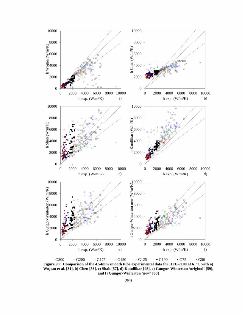
259
Figure 93: Comparison of the 4.54mm smooth tube experimental data for HFE-7100 at 61°C with a)
Wojtan et al. [31], b) Chen [56], c) Shah [57], d) Kandlikar [93], e) Gungor-Winterton ‘original’ [59],
and f) Gungor-Winterton ‘new’ [60]
0
2000
4000
6000
8000
10000
0 2000 4000 6000 8000 10000
h W
ojt
an (
W/m
²K)
h exp. (W/m²K)
0
2000
4000
6000
8000
10000
0 2000 4000 6000 8000 10000
h C
hen
(W
/m²K
)
h exp. (W/m²K)
0
2000
4000
6000
8000
10000
0 2000 4000 6000 8000 10000
h S
hah
(W
/m²K
)
h exp. (W/m²K)
0
2000
4000
6000
8000
10000
0 2000 4000 6000 8000 10000
h K
and
likar
(W
/m²K
)
h exp. (W/m²K)
0
2000
4000
6000
8000
10000
0 2000 4000 6000 8000 10000
h G
ungo
r-W
inte
rto
n (
W/m
²K)
h exp. (W/m²K)
0
2000
4000
6000
8000
10000
0 2000 4000 6000 8000 10000
h G
ungo
r-W
inte
rto
n n
ew (
W/m
²K)
h exp. (W/m²K)
0
2000
4000
6000
8000
10000
0 2000 4000 6000 8000 10000
h C
hen
(W
/m²K
)
h exp. (W/m²K)
G300 G200 G175 G150 G125 G100 G75 G50
a) b)
c) d)
e) f)
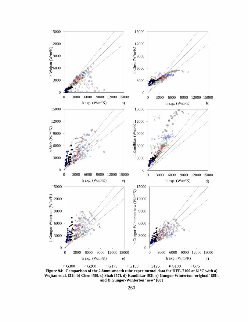
260
Figure 94: Comparison of the 2.8mm smooth tube experimental data for HFE-7100 at 61°C with a)
Wojtan et al. [31], b) Chen [56], c) Shah [57], d) Kandlikar [93], e) Gungor-Winterton ‘original’ [59],
and f) Gungor-Winterton ‘new’ [60]
0
3000
6000
9000
12000
15000
0 3000 6000 9000 12000 15000
h W
ojt
an (
W/m
²K)
h exp. (W/m²K)
0
3000
6000
9000
12000
15000
0 3000 6000 9000 12000 15000
h C
hen
(W
/m²K
)
h exp. (W/m²K)
0
3000
6000
9000
12000
15000
0 3000 6000 9000 12000 15000
h S
hah
(W
/m²K
)
h exp. (W/m²K)
0
3000
6000
9000
12000
15000
0 3000 6000 9000 12000 15000
h K
and
likar
(W
/m²K
)
h exp. (W/m²K)
0
3000
6000
9000
12000
15000
0 3000 6000 9000 12000 15000
h G
ungo
r-W
inte
rto
n (
W/m
²K)
h exp. (W/m²K)
0
3000
6000
9000
12000
15000
0 3000 6000 9000 12000 15000
h G
ungo
r-W
inte
rto
n n
ew (
W/m
²K)
h exp. (W/m²K)
0
2000
4000
6000
8000
10000
0 2000 4000 6000 8000 10000
h C
hen
(W
/m²K
)
h exp. (W/m²K)
G300 G200 G175 G150 G125 G100 G75 G50
a) b)
c) d)
e) f)

261
Figure 95: Comparison of the 8.84mm internally-grooved tube experimental data for HFE-7100 at
61°C with a) the Modified Sharar and Bar-Cohen correlation, and correlations from b) Thome et al.
[91], c) Cavallini et al. [117], d) Chamra and Mago [162], e) Wu et al. [103], and f) Yun et al. [90]
0
2000
4000
6000
8000
10000
0 2000 4000 6000 8000 10000
h S
har
ar a
nd
Bar
-Co
hen
(W
/m²K
)
h exp. (W/m²K)
0
2000
4000
6000
8000
10000
12000
14000
16000
18000
20000
0 2000 4000 6000 8000 10000
h T
ho
me
(W/m
²K)
h exp. (W/m²K)
0
2000
4000
6000
8000
10000
0 2000 4000 6000 8000 10000
h C
aval
lini
(W/m
²K)
h exp. (W/m²K)
0
2000
4000
6000
8000
10000
0 2000 4000 6000 8000 10000
h C
ham
ra (
W/m
²K)
h exp. (W/m²K)
0
2000
4000
6000
8000
10000
0 2000 4000 6000 8000 10000
h W
u (
W/m
²K)
h exp. (W/m²K)
0
2000
4000
6000
8000
10000
0 2000 4000 6000 8000 10000
h Y
un (
W/m
²K)
h exp. (W/m²K)
0
1000
2000
3000
4000
5000
6000
7000
8000
9000
10000
0 2000 4000 6000 8000 10000
h p
red
(W
/m²K
)
h exp (W/m²K)
G300 G200 G175 G150 G125 G100 G75 G50 G25
f) e)
c) d)
b) a)

262
Figure 96: Comparison of the 4.54mm internally-grooved tube experimental data for HFE-7100 at
61°C with a) the Modified Sharar and Bar-Cohen correlation, and correlations from b) Thome et al.
[91], c) Cavallini et al. [117], d) Chamra and Mago [162], e) Wu et al. [103], and f) Yun et al. [90]
0
3000
6000
9000
12000
15000
0 3000 6000 9000 12000 15000
h S
har
ar a
nd
Bar
-Co
hen
(W
/m²K
)
h exp. (W/m²K)
0
3000
6000
9000
12000
15000
18000
21000
24000
0 3000 6000 9000 12000 15000
h T
ho
me
(W/m
²K)
h exp. (W/m²K)
0
3000
6000
9000
12000
15000
0 3000 6000 9000 12000 15000
h C
aval
lini
(W/m
²K)
h exp. (W/m²K)
0
3000
6000
9000
12000
15000
0 3000 6000 9000 12000 15000
h C
ham
ra (
W/m
²K)
h exp. (W/m²K)
0
3000
6000
9000
12000
15000
0 3000 6000 9000 12000 15000
h W
u (
W/m
²K)
h exp. (W/m²K)
0
3000
6000
9000
12000
15000
0 3000 6000 9000 12000 15000
h Y
un (
W/m
²K)
h exp. (W/m²K)
0
2000
4000
6000
8000
10000
0 2000 4000 6000 8000 10000
h C
hen
(W
/m²K
)
h exp. (W/m²K)
G300 G200 G175 G150 G125 G100 G75 G50
a) b)
c) d)
e) f)

263
Figure 97: Comparison of the 2.62mm internally-grooved tube experimental data for HFE-7100 at
61°C with a) the Modified Sharar and Bar-Cohen correlation, and correlations from b) Thome et al.
[91], c) Cavallini et al. [117], d) Chamra and Mago [162], e) Wu et al. [103], and f) Yun et al. [90]
0
3000
6000
9000
12000
15000
0 3000 6000 9000 12000 15000
h S
har
ar a
nd
Bar
-Co
hen
(W
/m²K
)
h exp. (W/m²K)
0
3000
6000
9000
12000
15000
18000
21000
24000
27000
30000
33000
36000
0 3000 6000 9000 12000 15000
h T
ho
me
(W/m
²K)
h exp. (W/m²K)
0
3000
6000
9000
12000
15000
0 3000 6000 9000 12000 15000
h C
aval
lini
(W/m
²K)
h exp. (W/m²K)
0
3000
6000
9000
12000
15000
0 3000 6000 9000 12000 15000
h C
ham
ra (
W/m
²K)
h exp. (W/m²K)
0
3000
6000
9000
12000
15000
0 3000 6000 9000 12000 15000
h W
u (
W/m
²K)
h exp. (W/m²K)
0
3000
6000
9000
12000
15000
0 3000 6000 9000 12000 15000
h Y
un (
W/m
²K)
h exp. (W/m²K)
0
2000
4000
6000
8000
10000
0 2000 4000 6000 8000 10000
h C
hen
(W
/m²K
)
h exp. (W/m²K)
G300 G200 G175 G150 G125 G100 G75 G50
a) b)
c) d)
e) f)
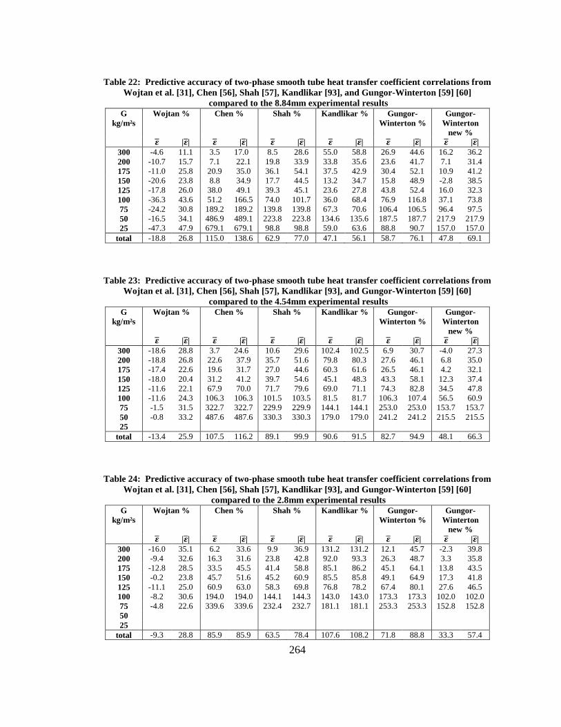
264
Table 22: Predictive accuracy of two-phase smooth tube heat transfer coefficient correlations from
Wojtan et al. [31], Chen [56], Shah [57], Kandlikar [93], and Gungor-Winterton [59] [60]
compared to the 8.84mm experimental results
G
kg/m²s
Wojtan % Chen % Shah % Kandlikar % Gungor-
Winterton %
Gungor-
Winterton
new %
𝜺 |𝜺| 𝜺 |𝜺| 𝜺 |𝜺| 𝜺 |𝜺| 𝜺 |𝜺| 𝜺 |𝜺|
300 -4.6 11.1 3.5 17.0 8.5 28.6 55.0 58.8 26.9 44.6 16.2 36.2
200 -10.7 15.7 7.1 22.1 19.8 33.9 33.8 35.6 23.6 41.7 7.1 31.4
175 -11.0 25.8 20.9 35.0 36.1 54.1 37.5 42.9 30.4 52.1 10.9 41.2
150 -20.6 23.8 8.8 34.9 17.7 44.5 13.2 34.7 15.8 48.9 -2.8 38.5
125 -17.8 26.0 38.0 49.1 39.3 45.1 23.6 27.8 43.8 52.4 16.0 32.3
100 -36.3 43.6 51.2 166.5 74.0 101.7 36.0 68.4 76.9 116.8 37.1 73.8
75 -24.2 30.8 189.2 189.2 139.8 139.8 67.3 70.6 106.4 106.5 96.4 97.5
50 -16.5 34.1 486.9 489.1 223.8 223.8 134.6 135.6 187.5 187.7 217.9 217.9
25 -47.3 47.9 679.1 679.1 98.8 98.8 59.0 63.6 88.8 90.7 157.0 157.0
total -18.8 26.8 115.0 138.6 62.9 77.0 47.1 56.1 58.7 76.1 47.8 69.1
Table 23: Predictive accuracy of two-phase smooth tube heat transfer coefficient correlations from
Wojtan et al. [31], Chen [56], Shah [57], Kandlikar [93], and Gungor-Winterton [59] [60]
compared to the 4.54mm experimental results
G
kg/m²s
Wojtan % Chen % Shah % Kandlikar % Gungor-
Winterton %
Gungor-
Winterton
new %
𝜺 |𝜺| 𝜺 |𝜺| 𝜺 |𝜺| 𝜺 |𝜺| 𝜺 |𝜺| 𝜺 |𝜺|
300 -18.6 28.8 3.7 24.6 10.6 29.6 102.4 102.5 6.9 30.7 -4.0 27.3
200 -18.8 26.8 22.6 37.9 35.7 51.6 79.8 80.3 27.6 46.1 6.8 35.0
175 -17.4 22.6 19.6 31.7 27.0 44.6 60.3 61.6 26.5 46.1 4.2 32.1
150 -18.0 20.4 31.2 41.2 39.7 54.6 45.1 48.3 43.3 58.1 12.3 37.4
125 -11.6 22.1 67.9 70.0 71.7 79.6 69.0 71.1 74.3 82.8 34.5 47.8
100 -11.6 24.3 106.3 106.3 101.5 103.5 81.5 81.7 106.3 107.4 56.5 60.9
75 -1.5 31.5 322.7 322.7 229.9 229.9 144.1 144.1 253.0 253.0 153.7 153.7
50 -0.8 33.2 487.6 487.6 330.3 330.3 179.0 179.0 241.2 241.2 215.5 215.5
25
total -13.4 25.9 107.5 116.2 89.1 99.9 90.6 91.5 82.7 94.9 48.1 66.3
Table 24: Predictive accuracy of two-phase smooth tube heat transfer coefficient correlations from
Wojtan et al. [31], Chen [56], Shah [57], Kandlikar [93], and Gungor-Winterton [59] [60]
compared to the 2.8mm experimental results
G
kg/m²s
Wojtan % Chen % Shah % Kandlikar % Gungor-
Winterton %
Gungor-
Winterton
new %
𝜺 |𝜺| 𝜺 |𝜺| 𝜺 |𝜺| 𝜺 |𝜺| 𝜺 |𝜺| 𝜺 |𝜺|
300 -16.0 35.1 6.2 33.6 9.9 36.9 131.2 131.2 12.1 45.7 -2.3 39.8
200 -9.4 32.6 16.3 31.6 23.8 42.8 92.0 93.3 26.3 48.7 3.3 35.8
175 -12.8 28.5 33.5 45.5 41.4 58.8 85.1 86.2 45.1 64.1 13.8 43.5
150 -0.2 23.8 45.7 51.6 45.2 60.9 85.5 85.8 49.1 64.9 17.3 41.8
125 -11.1 25.0 60.9 63.0 58.3 69.8 76.8 78.2 67.4 80.1 27.6 46.5
100 -8.2 30.6 194.0 194.0 144.1 144.3 143.0 143.0 173.3 173.3 102.0 102.0
75 -4.8 22.6 339.6 339.6 232.4 232.7 181.1 181.1 253.3 253.3 152.8 152.8
50
25
total -9.3 28.8 85.9 85.9 63.5 78.4 107.6 108.2 71.8 88.8 33.3 57.4

265
Table 25: Summary of the predictive accuracy of two-phase smooth tube heat transfer coefficient
correlations from Wojtan et al. [31], Chen [56], Shah [57], Kandlikar [93], and Gungor-Winterton
[59] [60] to the 2.8mm to 8.84mm experimental results
G
kg/m²s
Wojtan % Chen % Shah % Kandlikar % Gungor-
Winterton %
Gungor-
Winterton
new %
𝜺 |𝜺| 𝜺 |𝜺| 𝜺 |𝜺| 𝜺 |𝜺| 𝜺 |𝜺| 𝜺 |𝜺|
300 -13.1 25.0 4.5 25.2 9.67 31.6 96.2 97.5 15.3 40.3 3.3 34.4
200 -12.9 25.0 15.2 30.3 26.4 42.7 68.5 69.7 25.8 45.5 5.7 34.0
175 -13.7 25.6 24.6 37.4 34.8 52.5 60.9 63.5 34.1 54.1 9.6 38.9
150 -12.9 22.6 28.6 42.7 34.2 53.3 47.9 56.2 36.1 57.3 8.9 39.2
125 -13.5 24.4 54.4 59.8 56.4 64.8 56.5 59.1 61.8 71.7 26.1 42.2
100 -18.7 32.8 110.3 153.0 106.5 116.5 86.8 97.6 118.8 132.5 65.2 78.8
75 -10.2 28.3 274.1 274.1 200.7 200.8 130.8 131.9 204.2 204.3 134.3 134.6
50 -8.6 33.6 487.2 488.4 277.1 277.1 156.8 157.3 214.4 214.4 216.7 216.7
25 -47.3 47.9 679.1 679.1 98.8 98.8 59.0 63.6 88.7 90.7 157.0 157.0
total -14.0 26.9 100.7 115.6 72.8 85.9 80.6 84.4 72.1 87.5 44.3 65.3
Table 26: Predictive accuracy of the Modified Sharar and Bar-Cohen internally-grooved tube
correlation, and correlations from Thome et al. [91], Cavallini et al. [117], Chamra and Mago [162],
Wu et al. [103], and Yun et al. [90] compared to the 8.84mm experimental results
G Modified % Thome % Cavallini % Chamra % Wu % Yun %
kg/m²s 𝜺 |𝜺| 𝜺 |𝜺| 𝜺 |𝜺| 𝜺 |𝜺| 𝜺 |𝜺| 𝜺 |𝜺|
300 0.1 16.7 1.0 17.0 -35.8 48.4 111.9 192.5 -34.9 38.0 4.6 34.1
200 0.5 15.5 6.8 15.5 -43.0 50.1 -32.2 63.4 -46.3 47.8 -40.3 56.4
175 -5.2 17.8 12.5 21.8 -47.9 51.3 -43.9 59.1 -46.4 54.3 -55.5 58.9
150 -4.9 23.7 30.2 37.1 -42.3 57.6 70.8 177.0 -40.6 57.2 -55.7 68.0
125 -7.2 22.4 85.8 96.0 -44.9 55.8 -28.7 80.0 -21.2 83.7 -61.3 72.5
100 -17.6 35.0 137.6 147.0 -46.5 57.7 -38.3 77.5 -5.1 87.7 -71.0 76.2
75 -14.4 34.2 67.2 73.8 -34.8 56.2 -38.7 67.1 -37.8 60.8 -68.6 77.3
50 -38.4 47.4 224.3 225.1 11.7 70.9 -10.0 68.0 9.4 83.2 -66.5 72.7
25 -21.3 49.0 530.3 530.3 210.7 224.0 129.7 153.0 112.4 133.7 -48.3 73.0
total -10.8 27.5 93.7 101.9 -23.2 65.2 5.8 102.1 -20.7 68.3 -52.2 65.5
Table 27: Predictive accuracy of the Modified Sharar and Bar-Cohen internally-grooved tube
correlation, and correlations from Thome et al. [91], Cavallini et al. [117], Chamra and Mago [162],
Wu et al. [103], and Yun et al. [90] compared to the 4.54mm experimental results
G Modified % Thome % Cavallini % Chamra % Wu % Yun %
kg/m²s 𝜺 |𝜺| 𝜺 |𝜺| 𝜺 |𝜺| 𝜺 |𝜺| 𝜺 |𝜺| 𝜺 |𝜺|
300 -7.0 36.5 77.6 82.1 -38.9 42.3 -38.3 39.3 16.7 67.1 -54.9 58.8
200 -1.9 27.5 72.3 77.6 -34.5 44.4 -25.7 56.6 -4.8 73.9 -64.1 66.5
175 -6.1 23.2 104.6 108.0 -36.7 42.2 -40.2 45.5 1.3 86.7 -71.3 74.2
150 -3.5 18.3 39.8 44.0 -29.7 46.4 -22.0 63.8 -36.5 60.9 -70.5 75.9
125 15.3 33.6 129.7 134.2 -16.9 49.8 -26.2 51.0 -2.8 91.6 -70.5 78.1
100 6.2 24.1 256.0 260.0 -6.3 56.4 20.1 94.4 43.9 139.9 -71.9 80.5
75 8.3 27.3 139.3 142.4 24.1 70.9 41.4 104.0 -9.7 85.8 -66.0 84.4
50 12.5 34.9 277.2 279.6 141.5 167.5 161.6 197.0 35.9 107.9 -43.8 87.3
25
Total 2.0 28.1 125.9 130.0 -7.6 59.8 -0.2 74.5 3.7 86.7 -64.6 74.4

266
Table 28: Predictive accuracy of the Modified Sharar and Bar-Cohen internally-grooved tube
correlation, and correlations from Thome et al. [91], Cavallini et al. [117], Chamra and Mago [162],
Wu et al. [103], and Yun et al. [90] compared to the 2.62mm experimental results
G Modified % Thome % Cavallini % Chamra % Wu % Yun %
kg/m²s 𝜺 |𝜺| 𝜺 |𝜺| 𝜺 |𝜺| 𝜺 |𝜺| 𝜺 |𝜺| 𝜺 |𝜺|
300 -8.4 32.9 80.0 85.6 4.3 41.4 16.6 42.1 15.1 70.6 -57.0 73.1
200 4.7 32.3 123.1 131.2 19.5 49.5 25.2 47.9 17.6 97.9 -63.6 81.9
175 44.8 52.9 129.0 132.3 53.2 69.3 67.2 79.7 10.6 87.7 -64.5 77.2
150 73.5 80.8 228.7 233.9 61.0 74.7 62.1 73.1 50.2 133.9 -65.8 79.4
125 24.3 31.1 65.1 66.1 59.6 77.1 51.5 68.1 -29.2 56.0 -62.5 83.2
100 22.3 34.0 195.5 201.4 109.3 118.1 110.9 119.7 18.1 108.0 -69.3 72.4
75 -2.4 33.7 184.5 188.9 257.8 261.7 192.8 198.4 -0.9 74.9 -47.1 80.1
50
25
total 21.4 42.0 132.0 136.8 63.1 83.9 62.0 78.4 11.1 87.6 -61.6 78.1
Table 29: Summary of the predictive accuracy of the Modified Sharar and Bar-Cohen internally-
grooved tube correlation, and correlations from Thome et al. [91], Cavallini et al. [117], Chamra and
Mago [162], Wu et al. [103], and Yun et al. [90] for the 2.62mm to 8.84mm experimental results
G Modified % Thome % Cavallini % Chamra % Wu % Yun %
kg/m²s 𝜺 |𝜺| 𝜺 |𝜺| 𝜺 |𝜺| 𝜺 |𝜺| 𝜺 |𝜺| 𝜺 |𝜺|
300 -5.1 28.7 52.8 61.5 -23.4 44.0 30.0 91.3 -1.0 58.5 -35.7 55.3
200 1.1 25.1 67.3 74.7 -19.3 47.9 -10.9 55.9 -11.1 73.2 -55.9 68.3
175 11.2 31.3 82.0 87.3 -10.4 54.3 -5.6 61.4 -11.5 76.2 -63.7 70.1
150 21.7 40.9 99.5 105.0 -3.7 59.5 36.9 104.6 -8.9 84.0 -63.9 74.4
125 10.8 29.1 93.6 98.7 -0.7 60.9 -1.1 66.3 -17.7 77.1 -64.7 77.9
100 3.6 31.0 196.3 202.8 18.8 77.4 30.8 97.2 18.9 111.8 -70.7 76.4
75 -2.8 31.7 130.3 135.0 82.3 129.6 65.1 123.1 -16.1 73.8 -60.6 80.6
50 -12.9 41.1 250.7 252.3 76.6 119.2 75.8 132.5 22.6 95.5 -55.1 79.9
25 -21.3 48.9 530.3 530.3 210.7 223.9 129.7 152.9 112.4 133.7 -48.3 73.0
total 4.0 32.0 118.7 124.6 12.6 72.3 25.4 88.9 -2.4 80.7 -58.2 71.85

267
Chapter 10: Works Cited
[1] C. Mi, M. A. Masrur and D. Gao, Hybrid Electric Vehicles: Principles and
applications with practical perspectives, West Sussex: John Wiley and Sons Ltd.,
2011.
[2] B. Robinson, "defensesystems.com," 26 February 2010. [Online]. Available:
http://www.defensesystems.com/Articles/2010/03/11/Defense-IT-3-Greens.aspx.
[Accessed 2 August 2012].
[3] "U.S. Department of Energy: Energy Efficiency and Renewable Energy," 7
December 2010. [Online]. Available:
http://www1.eere.energy.gov/vehiclesandfuels/resources/fcvt_plans_roadmaps.ht
ml. [Accessed 3 August 2012].
[4] S. Garimella and V. Singhal, "Single-phase flow and heat transport in microchannel
heat sinks," 1st International Conference on Microchannels and Minichannels,
April 2003.
[5] C. Coutteau, "Advanced planning briefing to industry (APBI), TARDEC ground
vehicle power and mobility (GVPM)," US Army RDECOM-TARDEC, Warren,
Michigan, October 2008.
[6] I. Mudawar, "Assessment of high-heat-flux thermal management schemes," IEEE
Transactions on Components and Packaging Technologies, vol. 24, no. 2, pp. 122-
141, June 2001.
[7] D. Saums, "Vaporizable dielectric fluid cooling of IGBT power semiconductors for
vehicle powertrains," 6th International Conference on Integrated Power
Electronics Systems, pp. pp. 437-444, 2010.
[8] D. Sharar, N. Jankowski, B. Morgan and A. Bar-Cohen, "Two-phase minichannel
cold plate for Army vehicle power electronics," ASME InterPACK, vol. 2, pp. 133-
142, 2011.
[9] A. Bergles, "Heat transfer enhancement - the encouragement and accommodation
of high heat fluxes," Journal of Heat Transfer, vol. 119, pp. 8-19, 1997.
[10] A. Bergles, "Techniques to enhance heat transfer," in Handbook of Heat Transfer,
New York, NY, McGraw-Hill, 1998.
[11] J. Thome, Enhanced Boiling Heat Transfer, CRC Press, 1990.
[12] R. Webb, Principles of Enhanced Heat Transfer, New York, NY: John Wiley and
Sons, Inc., 1994.
[13] S. Kandlikar and P. Spiesman, "Augmentation of saturated flow boiling heat
transfer," in Chapter 18, Handbook of Phase Change, Philadelphia, PA, Taylor and
Francis, 1999.
[14] G. Moreno, S. Naramanchi, S. Thiagarajan, K. Bennion and T. Venson, "Enhanced
surfaces to improve power electronics cooling," in MEPTEC, San Jose, 2011.

268
[15] S. Yilmaz, J. Hwalck and J. Westwater, "Pool boiling heat transfer performance for
commercial enhanced tube surfaces," ASME Paper 90-HT-41, 1980.
[16] H. Kim, J. Kim and M. Kim, "Effect of nanoparticles on CHF enhancement in pool
boiling of nano-fluids," International Journal of Heat and Mass Transfer, vol. 49,
pp. 5070-5074, 2006.
[17] J. Thome, "Chapter 11: Boiling heat transfer inside enhanced tubes," in Wolverine
Engineering Data Book III, 2004.
[18] M. Jensen and H. Bensler, "Saturated forced-convection boiling heat transfer with
twisted-tape inserts," Journal of Heat Transfer, vol. 108, pp. 93-99, 1986.
[19] S. Laohalertdecha and S. Wongwises, "An experimental study into the evaporation
heat transfer and flow characteristics of R-134a refrigerant flowing through
corrugated tubes," International Journal of Refrigeration, vol. 34, pp. 280-291.
[20] D. Sharar, J. Nicholas, B. Morgan and A. Bar-Cohen, "Enhanced Two-Phase
Cooling," in IMAPS 2012 Chesapeake Chapter, College Park, MD, 2012.
[21] M. Houfuku, "Development trends in inner-grooved tubes in Japan," Hitachi Cable
Review, vol. 26, pp. 1-3, 2007.
[22] "Inner-grooved tubes," Wieland, [Online]. Available: http://www.wieland-
thermalsolutions.com/internet/en/branchenprodukte/kltetechnik/kaltwasserstze/inn
enberippterohre/Innenberippte_Rohre.jsp. [Accessed 18 January 2013].
[23] C. Dang, N. Haraguchi and E. Hihara, "Flow boiling heat transfer of carbon dioxide
inside a small-sized microfin tube," International Journal of Refrigeration, vol. 33,
pp. 655-663, 2012.
[24] L. Gao, Y. Watanabe and T. Honda, "CO2 flow boiling in small diameter smooth
and microfin tubes," Journal of JSEM, vol. 11, pp. 66-72, 2011.
[25] F. P. Incropera, D. P. Dewitt, T. L. Bergman and A. S. Lavine, Fundamentals of
Heat and mass Transfer, 6th ed., Hoboken: John Wiley & Sons,, 2007.
[26] M. Kim and J. Shin, "Evaporating heat transfer of R22 and R410A in horizontal
smooth and microfin tubes," International Journal of Refrigeration, vol. 28, pp.
940-948, 2005.
[27] T. Shedd and T. Newell, "Visualization of two-phase flow through microgrooved
tubes for understanding enhanced heat transfer," International Journal of Heat and
Mass Transfer, vol. 46, pp. 4169-4177, 2003.
[28] T. Ravigururajan and A. Bergles, "General correlations for pressure drop and heat
transfer for single-phase turbulent flow in internally ribber tubes," Augmentation of
Heat Transfer in Energy Systems, vol. 52, pp. 9-20, 1985.
[29] D. Sharar, N. Jankowski and A. Bar-Cohen, "Modified model for improved flow
regime prediction in internally-grooved tubes," in InterPACK, Burlingame, CA,
2013.
[30] L. Wojtan, T. Ursenbacher and J. Thome, "Investigation of flow boiling in
horizontal tubes: Part I - A new diabatic two-phase flow pattern map," International
Journal of Heat and Mass Transfer, vol. 48, pp. 2955-2969, 2005.
269
[31] L. Wojtan, T. Ursenbacher and J. Thome, "Investigation of flow boiling in
horizontal tubes: Part II - Development of a new hea ttransfer model for stratified-
wavy, dryout, and mist flow regimes," International Journal of Heat and Mass
Transfer, vol. 48, pp. 2970-2985, 2005.
[32] L. Cheng, G. Ribatski and J. Thome, "Two-phase flow patterns and flow-pattern
maps: Fundamentals and applications," Applied Mechanics Reviews, vol. 61, no. 5,
p. 28, 2008.
[33] J. Thome, A. Bar-Cohen, R. Revellin and I. Zun, "Unified mechanistic multiscale
mapping of two-phase flow patterns in microchannels," Experimental Thermal and
Fluid Science, vol. 44, pp. 1-22, 2013.
[34] V. Carey, Liquid vapor phase change phenomena, Washington D.C.: Hemisphere,
1992.
[35] A. Bar-Cohen and E. Rahim, "Modeling and prediction of two-phase microgap
channel heat transfer characteristics," Heat Transfer Engineering, vol. 30, no. 8, pp.
601-625, 2009.
[36] M. Cortina-Diaz and J. Schmidt, "Flow boiling heat transfer of n-Hexane and n-
Octane in a minichannel," in 13th International Heat Transfer Conference, Sydney,
Australia, 2006.
[37] Y. Yang and Y. Fujita, "Flow boiling heat transfer and flow pattern in rectangular
channel of mini-gap," in Proc. 2nd International Conference on Microchannels and
Minichannels, New York, USA, 2004.
[38] E. Bandarra Filho and J. Saiz Jabardo, "Convectiev boiling performance of
refrigerant R-134a in herringbone and microfin copper tubes," International
Journal of Refrigeration, vol. 29, pp. 81-91, 2006.
[39] J. Thome and G. Ribatski, "State-of-the-art of two-phase flow and flow boiling heat
transfer and pressure drop of CO2 in macro- and micro-channels," International
Journal of Refrigeration, vol. 28, pp. 1149-1168, 2005.
[40] L. Cheng, G. Ribatski, J. Quiben and J. Thome, "New prediction methods for CO2
evaporation inside tubes: Part I - A two-phase flow pattern map and a flow pattern
based phenomenological model for two-phase flow frictional pressure drops,"
International Journal of Heat and Mass Transfer, vol. 51, pp. 111-124, 2008.
[41] L. Cheng, G. Ribatski, L. Wojtan and J. Thome, "New flow boiling heat transfer
model and flow pattern map for carbond dioxide evaporating inside horizontal
tubes," International Journal of Heat and Mass Transfer, vol. 49, pp. 4082-4094,
2006.
[42] O. Baker, "Simultaneous Flow of Oil and Gas," Oil and Gas Journal, vol. 53, no.
12, pp. 185-195, 1954.
[43] J. Mandhane, G. Gregory and K. Aziz, "A flow pattern map for gas liquid flow in
horizontal pipes," International Journal of Multiphase Flow, vol. 1, no. 4, pp. 537-
553, 1974.

270
[44] Y. Taitel and A. Dukler, "A model for predicting flow regime transitions in
horizontal and near horizontal gas-liquid flow," AiChE Journal, vol. 22, no. 1, pp.
47-55, 1976.
[45] J. Weisman, D. Duncan, J. Gibson and T. Crawford, "Effect of fluid properties and
pipe diameter on two-phase flow pattern in horizontal lines," Internation Journal
of Multiphase Flow, vol. 5, no. 6, pp. 437-462, 1979.
[46] Y. Taitel, "Flow pattern transition in two phase flow," Proc. in 9th International
Heat Transfer Conference, pp. 237-254, 1990.
[47] N. Kattan, J. Thome and D. Favrat, "Flow boiling in horizontal tubes. Part I:
Development of a diabatic two-phase flow pattern map," Journal of Heat Transfer,
vol. 120, no. 1, pp. 140-147, 1998.
[48] O. Zurcher, J. Thome and D. Favrat, "Evaporation of ammonia in a smooth
horizontal tube: Heat transfer measurements and predictions," Journal of Heat
Transfer, vol. 121, pp. 89-101, 1999.
[49] O. Zurcher, D. Favrat and J. Thome, "Development of a diabatic two-phase flow
pattern map for horizontal flow boiling," International Journal of Heat and Mass
Transfer, vol. 45, pp. 291-301, 2002.
[50] J. Thome and J. El Hajal, "Two-phase flow pattern map for evaporation in
horizontal tubes: Latest version," Heat Transfer Engineering, vol. 24, no. 6, pp. 3-
10, 2003.
[51] F. Mancini, S. Minetto and E. Fornasieri, "Thermodynamic analysis and
experimental investigation of CO2 household heat pump dryer," International
Journal of Refrigeration, vol. 34, pp. 851-858, 2011.
[52] H. Abou-Ziyan, M. Ahmed, M. Metwally and H. Abd El-Hameed, "Solar assisted
R22 and R134a heat pump systems for low-temperature applications," Applied
Thermal Engineering, vol. 17, pp. 455-469, 1997.
[53] A. Diani, S. Mancin and L. Rossetto, "R1234ze(E) flow boiling inside a 3.4 mm ID
microfin tube," International Journal of Refrigeration, 2014.
[54] R. Mastrullo, A. Mauro, J. Thome, D. Toto and G. Vanoli, "Flow pattern maps for
convective boiling of CO2 and R410A in a horizontal smooth tube: Experiments
and new correlations analyzing the effect of reduced pressure," International
Journal of Heat and Mass Transfer, vol. 55, no. 5-6, pp. 1519-1528, 2012.
[55] E. Rahim, R. Revellin, J. Thome and A. Bar-Cohen, "Characterization and
prediction of two-phase flow regimes in miniature tubes," International Journal of
Multiphase Flow, vol. 37, pp. 12-23, 2011.
[56] J. Chen, "Correlation for boiling heat transfer to saturated fluids in convective
flow," Industrial and Engineering Chemistry - Process Design and Development,
vol. 5, pp. 322-329, 1966.
[57] M. Shah, "A new correlation for heat transfer during boiling flow through pipes,"
ASHRAE Transactions, vol. 82, pp. 66-86, 1976.

271
[58] S. Kandlikar and P. Balasubramanian, "An extension of the flow boiling correlation
to transition, laminar, and deep laminar flows in minichannels and microchannels,"
Heat Transfer Engineering, vol. 25, pp. 86-93, 2004.
[59] K. Gungor and R. Winterton, "A general correlation for flow boiling in tubes and
annuli," International Journal of Heat and Mass Transfer, vol. 29, pp. 351-358,
1986.
[60] K. Gungor and R. Winterton, "Simplified general correlation for saturated flow
boiling and comparisons of correlations with data," Chemical Engineering
Research and Design, vol. 65, pp. 148-156, 1987.
[61] N. Kattan, J. Thome and D. Favrat, "Flow boiling in horizontal tubes - Part II: New
heat transfer for five refrigerants," ASME Journal of Heat Transfer, vol. 120, pp.
148-155, 1998.
[62] N. Kattan, J. Thome and D. Favrat, "Flow boiling in horizontal tubes - Part III:
Development of a new heat transfer model based on flow patterns," ASME Journal
of Heat Transfer, vol. 120, pp. 156-165, 1998.
[63] A. Bergles and R. Manglik, "Current progress and new developments in enhanced
heat and mass transfer," Journal of Enhanced Heat Transfer, vol. 20, no. 1, pp. 1-
15, 2013.
[64] D. Sharar and A. Bar-Cohen, "Two-phase flow regimes and evaporative heat
transfer in internally-grooved tubes," Journal of Enhanced Heat Transfer , vol. 21,
no. 2-3, pp. 195-230, 2014.
[65] L. Liebenberg and J. Meyer, "Objective classification of two-phase flow regimes,"
Heat Transfer Engineering, vol. 29, no. 1, pp. 1-2, 2008.
[66] M. Yu, T. Lin and C. Tseng, "Heat transfer and flow pattern during two-phase flow
boiling of R-134a in horizontal smooth and microfin tubes," International Journal
of Refrigeration, vol. 25, pp. 789-798, 2002.
[67] S. Oh and A. Bergles, "Visualization of the effects of spiral angle on the
enhancement of in-tube flow boiling in microfin tubes," ASHRAE Trans., vol. 108,
no. 2, pp. 509-515, 2002.
[68] T. Shedd, T. Newell and P. K. Lee, "The effects of the number and angle of
microgrooves on the liquid film in horizontal annular two-phase flow,"
International Journal of Heat and Mass Transfer, vol. 46, pp. 4179-4189, 2003.
[69] B. Shen and E. Groll, "A critical review of the influence of lubricants on the heat
transfer and pressure drop of refrigerants, Part I: Lubricant influence on pool and
flow boiling," Internation Journal of HVAC&R Research, vol. 11, no. 3, pp. 341-
359, 2005.
[70] A.-E. Schael and M. Kind, "Flow pattern and heat transfer characteristics during
flow boiling of CO2 in a horizontal micro fin tube and comparison with smooth
tube data," International Journal of Refrigeration, vol. 28, pp. 1186-1195, 2005.
[71] J. Cho and M. Kim, "Experimental studies on the evaporative heat transfer and
pressure drop of CO2 in smooth and micro-fin tubes of the diameters of 5 and 9.52
mm," International Journal of Refrigeration, vol. 30, pp. 986-994, 2007.

272
[72] W. Targanski and J. Cieslinski, "Evaporation of R407C/oil mixtures inside
corrugated and micro-fin tubes," Applied Thermal Engineering, vol. 27, pp. 2226-
2232, 2007.
[73] H. Hu, G. Ding and K. Wang, "Heat transfer characteristics of R41oA-oil mixture
flow boiling inside a 7mm straight microfin tube," International Journal of
Refrigeration, vol. 31, no. 6, pp. 1081-1093, 2008.
[74] K. Spindler and H. Muller-Steinhagen, "Flow boiling heat transfer of R134a and
R404A in a microfin tube at low mass fluxes and low heat fluxes," Heat Mass
Transfer, vol. 45, pp. 967-977, 2009.
[75] E. Filho and P. Barbieri, "Flow boiling performance in horizontal microfinned
copper tubes with the same geometric characteristics," Experimental Thermal and
Fluid Sciences, vol. 35, pp. 832-840, 2011.
[76] A. Padovan, D. Del Col and L. Rossetto, "Experimental study on flow boiling of
R134a and R410A in a horizontal microfin tube at high saturation temperatures,"
Applied Thermal Engineering, vol. 31, pp. 3814-3826, 2011.
[77] V. Hatamipour and M. Akhavan-Behabadi, "Visual study on flow patterns and heat
transfer during convective boiling inside horizontal smooth and microfin tubes,"
World Academy of Science, Engineering, and Technology, vol. 69, pp. 700-706,
2012.
[78] X. Zhao and P. Bansal, "Flow boiling heat transfer analysis of new experimental
data of CO2 in a micro-fin tube at -30C," International Journal of Thermal
Sciences, vol. 59, pp. 38-44, 2012.
[79] L. Colombo, A. Lucchini and A. Muzzio, "Flow patterns, heat transfer, and pressure
drop for evaporation and condensation of R134A in microfin tubes," International
Journal of Refrigeration, vol. 35, pp. 2150-2165, 2013.
[80] D. Sharar and A. Bar-Cohen, "Flow regimes and evaporative heat transfer
coefficients for flow boiling in smooth and internally-grooved tubes," in
ITHERM2016, Las Vegas, NV, USA, 2016.
[81] T. Shedd and T. Newell, "An automated optical liquid film thickness measurement
method," Masters Thesis, University of Illinois, Urbana, IL.
[82] T. Shedd and T. Newell, "Observation of the influence of helical microgrooves on
the behavior of Annular two-phase flow," in Zero Leakage - Minimum Charge,
Stockholm, Sweden, 213-220.
[83] H. Kimura and M. Ito, "Evaporating heat transfer in horizontal internal spiral-
grooved tubes in the region of low flow rates," JSME, vol. 24, no. 195, pp. 1602-
1607, 1981.
[84] M. Ito and H. Kimura, "Boiling heat transfer and pressure drop in internal spiral-
grooved rubes," JSME, vol. 22, pp. 1251-1257, 1979.
[85] S. Yoshida, T. Matsunaga, H. Hong and K. Nishikawa, "Heat trasnfer enhancement
in horizontal, spirally grooved evaporator tubes," JSME International Journal Ser
II, vol. 31, no. 3, pp. 505-512, 1988.

273
[86] S. Yoshida, T. Matsunaga, H. Hong and K. Nishikawa, "Heat transfer to refrigerants
in horizontal evaporator tubes with internal, spiral grooves," in ASME-JSME
Thermal Engineering Joint Conference, 1987.
[87] S. Cui, Y. Tan and Y. Lu, "Heat transfer and flow resistance of R-502 flow boiling
inside horizontal ISF tubes," in Multiphase flow and heat transfer: Second
international symposium, Hemisphere Publishing Corp., 1992, pp. 662-670.
[88] A. Liu and R. Winterton, "A general correlation for saturated and subcooled flow
boiling in tubes and annuli based on a nucleate pool boiling equation," International
Journal of Heat and Mass Transfer, vol. 34, no. 11, pp. 2759-2766, 1991.
[89] K. Murata, "A correlation for forced convective boiling heat transfer of binary
refrigerant mixtures: 2nd report, a spirally grooved tube," Trans. Jpn. Soc. Mech.
Eng. Ser. B, vol. 62, pp. 2732-2728, 1996.
[90] R. Yun, Y. Kim, K. Seo and H. Kim, "A generalized correlation for evaporation
heat transfer of refrigerants in micro-fin tubes," International Journal of Heat and
Mass Transfer, vol. 45, pp. 2003-2010, 2002.
[91] J. Thome, N. Kattan and T. Favrat, "Evaporation in micro-fin tubes: a generalized
prediction model," in Convective Flow and Pool Boiling Conference, Kloster, Irsee,
1997.
[92] S. Koyama, J. Yu, S. Momoki, T. Fujii and H. Honda, "Forced convective flow
boiling heat transfer of pure refrigerants inside a horizontal microfin tube," in
Engineering Foundation Conference on Convective Flow Boiling, Banff, Canada,
1995.
[93] S. Kandlikar, "A model for correlating flow boiling heat transfer in augmented
tubes and compact evaporators," Journal of Heat Transfer, vol. 113, pp. 966-972,
1991.
[94] C. Park and P. Hrnjak, "Flow boiling heat transfer of CO2 at low temperatures in a
horizontal smooth tube," Journal of Heat Transfer, vol. 127, pp. 1305-1312, 2005.
[95] T. Cubaud and C. Ho, "Transport of bubbles in square microchannels," Phys.
Fluids, vol. 16, pp. 4575-4585, 2004.
[96] A. Serizawa, Z. Feng and Z. Kawara, "Two-phase flow in microchannels,"
Experimental Thermal Fluid Science, vol. 26, pp. 703-714, 2002.
[97] L. Gao and T. Honda, "Experiments on flow boiling heat transfer of pure CO2 and
CO2-oil mixtures in horizontal smooth and microfin tubes," in International
Refrigeration and Air Conditioning Conference, 2006.
[98] L. Gao, T. Honda and S. Koyama, "Experiments on flow boiling heat transfer of
almost pure CO2 and CO2-oil mixtures in horizontal smooth and microfin tubes,"
HVAC&R Research, vol. 13, pp. 415-425, 2007.
[99] L. Gao, T. Ono and T. Honda, "Pressure drops of CO2 and oil mixtures in horizontal
smooth and micro-fin tube evaporators," in International Congress of Refrigeration
ICR07-B1-1262, Beijing, 2007.
[100] Y. Kim, J. Cho and M. Kim, "Experimental study on the evaporative heat transfer
and pressure drop of CO2 flowing upward in vertical smooth and micro-fin tubes

274
with the diameter of 5mm," International Journal of Refrigeration, vol. 31, pp. 771-
779, 2008.
[101] T. Ono, L. Gao and T. Honda, "Heat transfer and flow characteristics of flow boiling
of CO2-oil mixtures in horizontal smooth and micro-fin tubes," Heat Transfer -
Asian Research, vol. 39, no. 3, pp. 195-207, 2010.
[102] L. Cheng, G. Ribatski and J. Thome, "New prediction methods for CO2 evaporation
inside tubes: Part II - An updated general flow boiling heat transfer model based on
flow patterns," International Journal of Heat and Mass Transfer, vol. 51, pp. 125-
135, 2008.
[103] Z. Wu, Y. Wu and B. L. W. Sunden, "Convective vaporization in micro-fin tubes
of different geometries," Experimental Thermal Fluid Science, vol. 44, pp. 298-
308, 2013.
[104] S. Mancin, A. Diani and L. Rossetto, "R134a flow boiling heat transfer and pressure
drop inside a 3.4 mm ID microfin tube," in 68th Conference of the Italian Thermal
Machines Engineering Association, ATI2013, 2014.
[105] J. Thome, "Two-phase heat transfer using no-phase flow models?," Heat Transfer
Engineering, vol. 25, no. 6, pp. 1-2, 2014.
[106] S. Nozu and H. Honda, "Condensation of refrigerants in horizontal, spirally
grooved microfin tubes: numerical analysis of heat transfer in annular flow regime,"
Journal of Heat Transfer, vol. 122, pp. 80-91, 2000.
[107] H. Honda, H. Wang and S. Nozu, "A theoretical model of film condensation in
horizontal microfin tubes," Journal of Heat Transfer, vol. 124, pp. 94-101, 2002.
[108] H. Wang, H. Honda and S. Nozu, "Modified theoretical models of film
condensation in horizontal microfin tubes," International Journal of Heat and Mass
Transfer, vol. 45, pp. 1513-1523, 2002.
[109] H. Mori, S. Yoshida, S. Koyama, A. Miyara and S. Momoki, "Prediction of heat
transfer coefficients for refrigerants flowing in horizontal spirally grooved
evaporator tubes," in 2002 Japan Society of Refrigerating and Air Conditioning
Engineers Annual Conference, Okayama, Japan, 2002.
[110] H. Honda and Y. Wang, "Theoretical study of evaporation heat transfer in
horizontal microfin tubes: stratified flow model," International Journal of Heat and
Mass Transfer, vol. 47, pp. 3971-3983, 2004.
[111] O. Makishi, H. Honda and Y. Wang, "New theoretical models of evaporation heat
transfer in horizontal microfin tubes," International Journal of Heat and Mass
Transfer, vol. 49, pp. 2328-2336, 2006.
[112] Y. Wang, Y. Wang, G.-X. Wang and H. Honda, "Prediction of evaporation heat
transfer coefficient based on gas-liquid two-phase annular flow regime in horizontal
microfin tubes," Applied Thermal Engineering, vol. 29, pp. 2970-2976, 2009.
[113] S. Momoki, S. Higashiiue, T. Shigechi, H. Mori, Yamaguchi and T, "Prediction of
evaporation heat transfer coefficient of refrigerants inside a horizontal spirally
grooved tube based on flow regime information," in Transactions of the Japan
Society of Refrigerating and Air Conditioning Engineers, 2006.

275
[114] L. Liebenberg and J. Meyer, "Refrigerant condensation flow regimes in enhanced
tubes and their effect on heat transfer coefficients and pressure drops," Heat
Transfer Engineering, vol. 29, pp. 506-520, 2008.
[115] L. Doretti, C. Zilio, S. Mancin and A. Cavallini, "Condensation flow patterns inside
plain and microfin tubes: A review," International Journal of Refrigeration, vol.
36, pp. 567-587, 2013.
[116] P. Rollman and K. Spindler, "A new flow pattern map for flow boiling in microfin
tubes," International Journal of Multiphase Flow, vol. 72, pp. 181-187, 2015.
[117] A. Cavallini, D. Del Col, L. Doretti, G. Longo and L. Rosetto, "Refrigerant
vaporization inside enhanced tubes: a heat transfer model," in Eurotherm Seminar,
Grenoble, France, 1998.
[118] L. Liebenberg, J. Thome and J. Meyer, "Flow visualization and flow pattern
identification with power spectral density distributions of pressure traces during
refrigerant condensation in smooth and microfin tubes," Journal of Heat Transfer,
pp. 209-220, 2005.
[119] J. Thome, "Update on Kattan-Thome-Favrat flow boiling model and flow pattern
map," in 5th International conference on boiling heat transfer, 2003.
[120] J. Thome, J. El Hajal and A. Cavallini, "Condensation in horizontal tubes, part 2:
new heat transfer model based on flow regimes," International Journal of Heat and
Mass Transfer, vol. 46, pp. 3365-3387, 2003.
[121] D. Barnea, O. Shoham, Y. Taitel and A. Dukler, "Flow pattern transition for
downward inclined two phase flow; horizontal to vertical," Chem. Eng. Sci., vol.
37, pp. 735-740, 1982.
[122] D. Steiner, "Heat transfer to boiling saturated liquids," VDI-Warmeatlas (VDI Heat
Atlas.
[123] L. Wojtan, T. Ursenbacher and J. Thome, "Dynamic void fractions in stratified
types of flow, Part II: Measurements for R-22 and R-410A," Int. J. Multiphase
Flow, vol. 30, pp. 125-137, 2004.
[124] D. Biberg, "An explicit approximation for the wetted angle in two-phase stratified
pipe flow," Canadian Journal of Chemical Engineering, vol. 77, pp. 1221-1224,
1999.
[125] H. Mori, S. Yoshida, K. Ohishi and Y. Kokimoto, "Dryout quality and post dryout
heat transfer coefficient in horizontal evaporator tubes," in Proc. of 3rd European
Thermal Sciences Conference, 2000.
[126] S. Kutateladze, "On the transition to film boiling under natural convection,"
Kotloturbostroenie, vol. 3, no. 10, 1948.
[127] M. Cooper, "Saturated nucleate pool boiling: A simple correlation," in First UK
National Heat Transfer Conference, 1984.
[128] J. El Hajal, J. Thome and A. Cavallini, "Condensation in horizontal tubes, Part 2:
New heat transfer model based on flow regimes," International Journal of Heat and
Mass Transfer, vol. 46, no. 18, pp. 3365-3387, 2003.

276
[129] D. Groeneveld, "Post dry-out heat transfer at reactor operating conditions," in ANS
Topical Meeting on Water Reactor Safety, Salt Lake City, 1973.
[130] R. Dougall and W. Rohsenow, "Film boiling on the inside of vertical tubes with
upward flow of the fluid at low vapor qualities," MIT Report no. 9079-26, 1963.
[131] L. Wojtan, Experimental and analytical investigation of void fraction and heat
transfer during evaporation in horizontal tubes, Lausanne, Switzerland: PhD Thesis,
Department of Mechanical Engineering, Swiss Federal Institute of Technology,
2004.
[132] M. Lallemand, C. Branescu and P. Haberschill, "Local heat transfer coefficients
during boiling of R-22 and R-407C in horizontal smooth and microfin tubes,"
International Journal of Refrigeration, vol. 24, pp. 57-72, 2001.
[133] M. Steinke and S. Kandlikar, "Control and effect of dissolved air in water during
flow boiling in microchannels," International Journal of Heat and Mass Transfer,
vol. 47, pp. 1925-1935, 2003.
[134] A. Smith, N. Jankowski and L. Boteler, "Measurement of high performance thermal
interfaces using a reduced scale steady-state tester and infrared microscopy,"
Journal of Heat Transfer, Accepted manuscript posted December 7, 2015.
[135] J. Bennett and E. Ashley, "Infrared reflectance and emittance of silver and gold
evaporated in ultrahigh vacuum," Applied Optics, vol. 4, no. 2, pp. 221-224, 1965.
[136] O. Loebich, "The optical properties of gold," in Gold Bull, 1972, pp. 2-10.
[137] D. Sharar, A. Bergles, N. Jankowski and A. Bar-Cohen, "Non-intrusive optical
validation of two-phase flow regimes in a small diameter tube," in ASME FEDSM,
Chicago, 2014.
[138] T. Salem, D. Ibitayo and B. Geil, "Validation of infrared camera thermal
measurements on high-voltage power electronic components," IEEE Transactions
on Instrumentation and Measurement, vol. 56, no. 5, pp. 1973-1978, 2007.
[139] E. Rahim, "Limits of thin film cooling in microgap channels," Doctor of
Philosophy, UMD, Department of Mechanical Engineering, 2011.
[140] P. Bevington and D. Robinson, Data reduction and error analysis for the physical
sciences, McGraw-Hill Education; 3rd edition, 2002.
[141] A. Ullmann and B. Brauner, "The prediction of flow pattern maps in mini
channels," Multiphase Science Technology, vol. 19, no. 1, pp. 49-73, 2007.
[142] D. Sharar, A. Bergles, N. Jankowski and A. Bar-Cohen, "Non-intrusive optical
validation of two-phase flow regimes in a small diameter tube," Jouurnal of Heat
Transfer Engineering, vol. 37, no. 11, 2016.
[143] J. Drahos and J. Cermak, "Diagnostics of gas-liquid flow patterns in chemical
engineering systems," Chemical Engineering and Processing, vol. 26, no. 2, pp.
147-164, 1989.
[144] C. Owen, J. Jones and N. Zuber, "The interrelation between void fraction
fluctuations and flow patterns in two-phase flow," International Journal of
Multiphase Flow, pp. 273-306, 1975.

277
[145] M. Vince and R. Lahev, "On the development of an objective flow regime
indicator," International Journal of Multiphase Flow, pp. 93-124, 1982.
[146] R. Rahim and M. Rahiman, "Non-invasive imaging of liquid/gas flow using
ultrasonic transmission-mode tomography," Sensors and Actuators, pp. 337-345,
2007.
[147] J. Burns, C. Ramshaw and R. Jachuck, "Measurement of liquid film thickness and
the determination of spin-up radius on a rotating disc using an electrical resistance
technique," Chemical Engineering Science, pp. 2245-2253, 2003.
[148] H. Caniere, B. Bauwens, C. T'Joen and M. DePaepe, "Mapping of horizontal
refrigerant two-phase flow patterns based on clustering of capacitive sensor
signals," International Journal of Heat and Mass Transfer, pp. 5298-5307, 2010.
[149] R. Revellin, V. Dupont, T. Ursenbacher, J. Thome and I. Zun, "Characterization of
two-phase flows in microchannels: Optical measurement technique and flow
parameter results for R-134a in a 0.5mm channel," International Journal of
Multiphase Flow, vol. 32, pp. 755-774, 2006.
[150] E. Jassim, T. Newell and J. Chato, "Probabilistic determination of two-phase flow
regimes in horizontal tubes utilizing an automated image recognition technique,"
Experiments in Fluids, pp. 563-573, 2007.
[151] T. Ursenbacher and L. T. J. Wojtan, "Interfacial measurements in stratified types of
flow - Part 1: New optical measurement technique and dry angle measurement,"
Internationl Journal of Multiphase Flow, pp. 107-124, 2004.
[152] H. Canière, "Flow pattern mapping of horizontal evaporating refrigerant flow based
on capacitive void fraction measurements," Ph.D. Thesis, Ghent University -
UGent, Gent, Belgium, 2009.
[153] A. Pautsch and T. Shedd, "Adiabatic and diabatic measurements of the liquid film
thickness during spray cooling with FC-72," International Journal of Heat and
Mass Transfer, vol. 49, pp. 2610-2618, 2006.
[154] T. Shedd and T. Newell, "Automated optical liquid film thickness measurement
method," Review of Scientific Instruments, vol. 69, no. 12, pp. 4205-4213, 1998.
[155] S. Rouhani and M. Sohal, "Two-phase flow patterns: A review of research results,"
Prog. Nucl. Energy, vol. 11, no. 3, pp. 219-259, 1983.
[156] "OLS4000 Optical Metrology," Olympus, [Online]. Available:
http://www.olympus-ims.com/en/metrology/ols4000/. [Accessed 20 August 2013].
[157] "Norland Optical Adhesive 65," Norland Products, [Online]. Available:
https://www.norlandprod.com/adhesives/noa%2065.html. [Accessed 21 August
2013].
[158] K. Triplett, S. Ghiaasiaan, S. Abdel-Khalik and D. Sadowski, "Gas-Liquid two-
phase flow in micro-channels, part 1: two-phase flow pattern," Int. J. Multiphase
Flow, vol. 25, pp. 377-394, 1999.
[159] R. Revellin, "Experimental Two-phase Fluid Flow in Microchannels. PhD. Thesis
(Prof. John R. Thome, Director), LTCM-EPFL, Swiss Federal Institute of
Technology," 2005.

278
[160] R. da Silva Lima, J. Moreno Quiben and J. Thome, "Flow boiling in horizontal
smooth tubes: New heat transfer results for R-134a at three saturation
temperatures," Applied Thermal Engineering, vol. 29, no. 7, pp. 1289-1298, 2009.
[161] A. Bar-Cohen, C. Holloway, A. Riaz and A. Kaffel, "Waves and instabilities in high
quality adiabatic flow in microgap channels," International Journal of Multiphase
Flow, p. accepted for publication, 2016.
[162] L. Chamra and P. Mago, "Modelling of evaporation heat transfer of pure
refrigerants and refrigerant mixtures in microfin tubes," Journal of Mechanical
Engineering Science, vol. 221, no. Part C, pp. 443-454, 2007.
[163] E. Lemmon, M. Huber and M. McLinden, NIST Standard Reference Database 23:
Reference Fluid Thermodynamic and Transport Properties - REFPROP, Version
7.0, Gaithersburg: National Institute of Standards and Technology, Standard
Reference Data Program.
[164] H. Lin, P. Ye and G. Wilk, "Leakage current and breakdown electric-field studies
on ultrathin atomic-layer-deposited Al2O3 on GaAs," Applied Physics Letters, vol.
87.
[165] Y. Zhang, J. Bertrand, R. Yang and S. L. Y. George, "Electroplating to visualize
defects in Alumina thin films grown using atomic layer deposition," Thin Solid
Films, vol. 517, pp. 3269-3272, 2009.
[166] M. Kroll, W. Blau, R. Grandjean, F. Benfield, P. Lusi, L. Paulus and J. de Jongh,
"Magnetic properties of ferromagnetic nanowires embedded in nanoporous alumina
membranes," Journal of Magnetism and Magnetic Materials, vol. 249, pp. 241-245,
2002.
[167] M. Schlesinger and M. Paunovic, Modern Electroplating, New York: John Wiley
& Sons, 2000.
[168] Y. Zhang, D. Seghete, A. Abdulagatov, Z. Gibbs, A. Cavanagh, R. Yang, S. George
and Y. Lee, "Investigation of the defect density in ultra-thin Al2O3 films grown
using atomic layer deposition," Surface & Coatings Technology, vol. 205, pp. 3334-
3339, 2011.
[169] "Impreglon Worldwide Quality Coatings," [Online]. Available:
http://www.impreglon.us/front_content.php?changelang=3. [Accessed 2013].
[170] W.-S. Kwack, H.-J. Choi, W.-C. O. H.-R. Choi, S.-Y. M. K. K. J.-Y. Shin, Y.-K.
Jeong and S.-H. Kwon, "Charging characteristics of Ru Nanocrystals embedded in
Al2O3 matrix prepared by using the initial growth stage of Ru plasma-enhanced
atomic layer deposition," Journal of Ceramic Processing Research, vol. 13, no. 3,
pp. 338-342, 2012.
Top Related