


Languages
Pages
Legal


A Volumetric Approach to Rendering Microgeometry
Using PRT
by
John Kloetzli
Department of Computer Science & Electrical EngineeringUniversity of Maryland, Baltimore County
Baltimore, MD

Abstract
This paper introduces Precomputed Radiance Transfer (PRT) to shell textures in the
context of rendering microgeometry. PRT is a method which allows static objects to have
global illumination effects such as self shadowing and soft shadows while being rendered in
real-time. This is done by representing the object’s spherical ’light transfer function,’ which
captures how the object translates irradiance into radiant emittance, in a spherical/zonal har-
monic basis in order to allow approximate illumination in arbitrary lighting environments.
Shell textures is a technique for rendering complex surface geometry in real-time through
the use of concentric 3D rings or shells around a model. The shells are transparent every-
where except at the intersection of the shell and the microgeometry that is being rendered.
We novelly combine these two techniques to render realistic microgeometry with global
lighting effects at real-time frame rates.

TABLE OF CONTENTS
Chapter 1 INTRODUCTION . . . . . . . . . . . . . . . . . . . . . . . . 2
1.1 Previous Work . . . . . . . . . . . . . . . . . . . . . . . . . . . . . . . . . 3
Chapter 2 BACKGROUND . . . . . . . . . . . . . . . . . . . . . . . . . 5
2.1 Spherical Harmonics . . . . . . . . . . . . . . . . . . . . . . . . . . . . . 5
2.2 Zonal Harmonics Approximation . . . . . . . . . . . . . . . . . . . . . . . 8
2.3 Precomputed Radiance Transfer . . . . . . . . . . . . . . . . . . . . . . . 10
2.4 Local, Deformable Precomputed Radiance Transfer . . . . . . . . . . . . . 12
Chapter 3 METHOD . . . . . . . . . . . . . . . . . . . . . . . . . . . . . 15
3.1 Creating a realistic volumetric fur model . . . . . . . . . . . . . . . . . . . 15
3.2 Precomputing illumination of the fur volume . . . . . . . . . . . . . . . . 17
3.3 Rendering the volume . . . . . . . . . . . . . . . . . . . . . . . . . . . . . 19
3.4 Reconstructing the lighting . . . . . . . . . . . . . . . . . . . . . . . . . . 20
Chapter 4 RESULTS . . . . . . . . . . . . . . . . . . . . . . . . . . . . . 22
Chapter 5 CONCLUSIONS AND FUTURE WORK . . . . . . . . . . . . 26
REFERENCES . . . . . . . . . . . . . . . . . . . . . . . . . . . . . . . . . . . 28
1

Chapter 1
INTRODUCTION
Rendering microsurfaces is a difficult task in computer graphics. Because microsur-
faces are by definition very high frequency geometry, traditional rasterization or ray tracing
techniques bog down to the point of uselessness or are plagued with terrible aliasing arti-
facts. Surface shading techniques are also not suited to the task because microsurfaces,
although very small, are still geometrically visible to the naked eye, which lighting equa-
tions alone are unable to capture.
Fur is a perfect example of a microsurface, containing hundreds or thousands of hairs
that are very small but certainly individually visible. However, microgeometry in the con-
text of computer graphics extends beyond objects that actually contain ‘micro-scale’ detail
in the real world to include surfaces of similar structure at any scale. Grass, when viewed
from a sufficient height, can also be considered microgeometric because it exhibits the
same properties as the fur described above. Other examples at different scales include
thick tree cover, bushes, etc. Our rendering method works for all surfaces which exihibit
microgeometric properties at any scale.
2
1.1 Previous Work
Kajiya and Kay [1989] described a volumetric ray-tracing method for rendering fur
which stored the microsurface data in a volume and modeled light scattering and attenua-
tion along each ray through the volume. This method produced excellent results, but was
far from real-time. Hypertexture [Perlin and Hoffert, 1989] is a volume modeling method
that can be used to create fur. Instead of capturing actual surfaces in a volume they mod-
ulate density of voxels by combining different building-block functions in various ways.
This allows many interesting surfaces to be generated easily, but most rendering imple-
mentations do not attempt to account for intra-surface shadowing or reflectance. There
are implementations of Hypertexture that run in realtime on todays graphics hardware, but
none of them attempt to compute global lighting.
A real-time fur technique of interest here was introduced in 2001 by Lengyel et al
[2001]. The method creates concentric shells around the model being rendered, each shell
displaying a different part of a volume texture. The shells are transparent except for the
precomputed intersection of the shell and the fur volume that they created. When rendered
together they create a very convincing furry surface. This works well when viewed from
above since the shells overlap, creating the illusion of continuous geometry, but it doesn’t
work for facecs near the silhouette of the object since the gaps between adjacent shells
become apparent. To remedy this, they add small textures rendered normal to the surface
across all the edges in the model, which they fade in as the edge approaches the silhouette.
These fin textures fill in the gaps in the shell textures on the silhouette, creating a complete
geometric render of fur. This technique can be viewed as a form of rendering the Kajiya
and Kay [1989] fur model in real-time, but using a simple ambient/diffuse/specular lighting
scheme that doesn’t capture self shadowing. Real-time lighting of microsurfaces is a diffi-
cult problem, but one that must be solved to even approach realistic results. As discussed by
Lokovic and Veach [2000], rendering realistic microgeometry such as fur depends heavily
3
on inter-object shadows, namely hair-to-hair shadows.
Since asthetically pleasing fur illumination can be obtained in offline rendering [Ka-
jiya and Kay, 1989], one possible approach is to precompute the lighting at different points
on the object and recreate it at run time to approximate run-time lighting. Precomputed
Radiance Transfer [Sloan et al., 2002] allows for this through the use of basis functions
designed to efficiently encode the lighting across an object for later reconstruction. Several
different basis functions have been explored, including Spherical Harmonics (SH)[Sloan
et al., 2002; 2003], Zonal Harmonics (ZH)[Sloan et al., 2005], and Harr Wavelets (HW)
[Wang et al., 2005; Liu et al., 2004]. While SH and ZH are limited to low-frequency
lighting, they are very compact and are relatively fast. In addition, ZH representations can
be rotated into an arbitrary frame very quickly. The HW basis functions are much more
numerous, which allows them to represent all-frequency lighting, but also require more tex-
ture space and run-time processing. Usual implementations store lighting on a per-vertex
basis, but light-cloud representations [Kristensen et al., 2005] have also been used.
Many different variations of PRT have been explored. It has been used to recreate
diffuse and specular lighting[Sloan et al., 2002; Liu et al., 2004], as well model subsurface
scattering [Wang et al., 2005] in real-time. Multiple scales of PRT [Sloan et al., 2003] can
be used to create high-frequency local effects in addition to complete inter-model lighting.
Fast ZH rotation allows for easily rotated transfer functions, leading to PRT for deformable
objects [Sloan et al., 2005]. This method is different from other applications of PRT be-
cause it does not try to compute global lighting on an entire object, but only the sort of
global effects that appear relatively locally to points on the surface. No PRT methods al-
low for geometric deformation on the region of interest; ZH-based representations simply
restrict this region to a portion of a model instead of the whole.
4
Chapter 2
BACKGROUND
Our method relies heavily on the theory of Precompute Radiance Transfer (PRT) in-
troduced by Sloat et al [2005; 2002]. PRT is a very powerful technique because it allows
for global illumination effects in realtime under certain conditions. We believe that correct
shadows, which are a global illumination effect, are essential to realistic microgeometry.
Therefore, it is necessary to discuss in detail some of the mathematical basis for PRT and
how it has been applied in the past in order to understand how our method works.
2.1 Spherical Harmonics
The Spherical Harmonics (SH) are an infinite set of spherical functions that form
an orthonormal basis over the sphere. The SH function with parameters l : l ∈ N and
m :−l ≥ m≤ l is defined by
Y ml (θ ,ψ) =
√2l +1
4π· (l−m)!(l +m)!
· eimψ ·Pml (cos(θ)) (2.1)
where Pml are the associated Legendre polynomials. This formulation isn’t quite what we
want for this application, however, because it will contain imaginary numbers if m 6= 0. We
can remedy this by constructing the following piecewise defined function to take care of
those cases:
5

Y ml (θ ,ψ) =
√2 ·Km
l · cos(mψ) ·Pml (cos(θ)), i f m > 0
√2 ·Km
l · sin(−mψ) ·P−ml (cos(θ)), i f m < 0
K0l ·P0
l (cos(θ)), i f m = 0
(2.2)
where
Kml =
√2l +1
4π· (l−m)!(l +m)!
. (2.3)
The SH functions are applicable to our problem because they allow us to approximate
arbitrary spherical functions, which are used in the context of lighting to represent lighting
environments around a point in space. A sum of an unbounded number of SH basis func-
tions with the correct coefficients can approximate a function to any desired accuracy. This
can be thought of as a Fourier Transformation on a sphere, since we are approximating an
arbitrary function with sums of oscillating basis functions.
Several properties of the SH functions make them very convenient to use as a basis for
spherical light functions. First, the frequency of the activity in a SH function is preportional
to the order so if we are interested only in a rough, low frequency approximation we only
need to compute a fixed number of low-order SH functions to use as a basis. Second, SH
projection will act as a smooth bluring filter on our resulting lighting, which ensures that
our result will not have any noticable high-frequency artifacts. Third, addition/subtraction
of SH projections are completed with simple addition/subtraction of corresponding SH
coefficients, which is trivial to evaluate. Finally, provided that only the lowest 3-5 levels of
SH are used, complete spherical lighting environments projected into SH are very compact.
Even though there are many advantages to using the SH functions to represent light,
there are also several disadvantages. One of the most obvious is that SH approximations
that want to contain higher frequencies become too large to be practical since the number of
functions needed to represent those frequencies is very large. In addition, SH functions are6

plagued by the same ‘ringing’ artifacts that Fourier transforms exhibit under some circum-
stances. These effects are the worst when a large number of coefficients are used and/or
the function being projected contains a high-contrast step function in frequency space (see
Figure 2.1).
FIG. 2.1. From left to right: A spherical wedge function and its 2nd, 4th, 6th and 8thlevel SH projections with blue representing positive vales and red negative. Note that thefrequency and quality of the approximations increase from left to right. Also note thedevelopment of high-frequency noise in the higher order approximations near the sharpvalue change.
FIG. 2.2. The five lowest order Zonal Harmonic functions. Blue represents positive, rednegative.
7

2.2 Zonal Harmonics Approximation
Although SH functions are very convienient to represent light at points on a model,
they are not easy to rotate in arbitrary directions. In order to be able to do this, we have to
re-project our function from the SH basis into one that is easier to rotate. Zonal Harmonics
(ZH) are the subset of the spherical harmonics defined in (2.2) with m = 0, and are pictured
in Figure 2.2. The ZH functions are the only SH functions that are symetric about the ver-
tical axis and rotationally invariant (unchanged by rotation) around that axis. This property
means that we can rotate any ZH function and project the rotated ZH into the SH basis with
one simple formula [Sloan et al., 2005]. Let g be a sum of the n lowest-order ZH functions,
given by
g =n
∑l=1
glY 0l (2.4)
If f is a spherical function projected into the n lowest-order SH basis functions, then
f =n
∑l=1
l
∑m=−l
flmY ml (2.5)
Let f be a projection from a rotated version of g, which defines the relationship be-
tween f and g to be
f (z) = g(z) = g(R−1(z)) (2.6)
where R is a rotation from the horizonal axis z of g to an arbitrary axis z. Each
coefficient flm of the rotated SH function will be the sum of the coefficient of gl , a scaling
factor based on l, and the corresponding SH function evaluated in the direction of z. The
formula for this is given by
8
flm =
(gl
√2π
2l +1
)Y m
l (zl) = g∗l Y ml (zl) (2.7)
where
g∗l = gl
√2π
2l +1(2.8)
The important thing to notice about this equation is that the ZH functions associated
with each coefficient gl do not have to be rotated with the same zl, but each level of SH
with the same m do. In other words, each ZH function must be given some rotation zl
which must be used in the above formula for that entire level, but different levels can have
different zl.
This formula allows us to simultaneously rotate a ZH vector in an arbitrary direction
and project the result into the SH basis, but that is only half of what we need to do. We also
need to project a SH vector into the ZH basis, which is a much harder problem. Let f and
g be the spherical functions defined in equations (3) and (4), except here we want to find
the best g to approximate f . The equation that evaluates the L2 norm between f and g is
ψ =‖ f −g ‖ (2.9)
which will be the error metric for our approximation. However, this equation cannot be
evaluated directly because f is represented in SH and g in ZH. One efficient way to calcu-
late ψ is to project g into the SH bases by equation (2.7) to get g and subtract corresponding
coefficients. Therefore ψ is a minimization function with all components of g as variables.
However, the value of the SH coefficients for a single ZH with a fixed rotation z that mini-
mizes ψ has been found to be [Sloan et al., 2005]
9
g∗l =
4πl
∑m=−l
Y ml (z) flm
2l +1(2.10)
where g∗l is defined in (2.8). This effectivly means that the only variables in the error
equation (2.9) are the rotations on each level of ZH function, since the optimal coefficients
can be calculated given the rotation. Rather than solve this problem all at once, we can
solve it for each ZH level one at a time, subtracting out the best fit found so far from the
target SH vector. Because lower-order ZH functions are lower frequency and thus will
make the largest impact on minimizing (2.9), we perform this approximation for each level
ZH starting with the lowest.
We found that it was sufficient to simply calculate several hundred rotations uniformly
distributed on the hemisphere, solve (2.10) for each one and keep the rotation that produced
the lowest error. The ZH function with that rotation is then projected into the SH basis using
equation (2.7) and subtracted from the target SH vector f . This process is then repeated
with the next higher level ZH function and the new target vector. This gives us a close
approximation of our SH function f represented as a sum of rotated ZH basis functions.
Error analysis for this approximation was performed by Sloan [2005].
2.3 Precomputed Radiance Transfer
Precomputed Radiance Transfer (PRT) [Sloan et al., 2002] takes the principles of SH
function approximation and applies them to the problem of real-time global illumination.
Although there are many different versions of PRT that vary slightly in the details, the basic
idea of PRT is to represent the ‘light transfer function’ of an entity in the SH basis. Then,
if the lighting environment of the entity can also be represented in SH, final illumination of
the entity can be calculated with a simple dot product between the transfer and environment
SH vectors. The steps needed to perform this calculation are precomputation of the transfer
10
function, projecting the lighting environment of the entity into SH, and evaluating the final
lighting for the object.
Precomputing the transfer function of an entitiy is very straightforward. First the
desired global illumination techniques must be decided. Although the most commonly
cited application is to simply use radiosity to calculate global illumination, any type of
global lighting effect such as subsurface scattering, transluscence, or self reflection can be
used alone or together. View-dependent effects can be calculated, but at greater cost than
uniform effects. Our method does not use view-dependent illumination, so we will not
discuss that technique here. These lighting effects must be computed for each of the SH
functions that are going to be used. This is accomplished by representing the SH function
as light approaching the object from the infinate sphere and running the desired global
illumination algorithm. Because the SH functions contain negative values, the lighting
often has to be computed twice for each basis function: once with the positive light and
once with the opposite of the negative light. The final result can be attained by subtracting
the result from the negative light calculation from the positive light one. When this has
been completed for each basis function the result is a set of SH coefficients, which are real
numbers, representing the global light transfer of the entity under the SH basis functions.
Light in the environment must also be projected into the SH basis before evaluation
can take place. One nice feature of the SH basis is that adding two spherical functions in the
SH basis is as simple as adding their corresponding coefficients. This allows us to project
multiple lights from a scene into SH seperately and add them together in SH space, which is
trivial. If the light in the environment is dynamic then the light projection calculation must
take place at least partly per-frame. Projecting an arbitrary spherical environment into the
SH basis is expensive. Given a spherical function h the coefficient for a particular band of
SH Y ml is given by the integral over the sphere S of the product of the two functions.
11
cml =
∫
Sh(S)Y m
l (S)ds (2.11)
Standard approximate integration techniques [Green, 2003] allow us to write this in
summation form over a set of n uniformly distributed random samples on S, denoted by the
vector X = x1,x2, ...xn.
cml =
4πn
n
∑i=1
hY ml (xi) (2.12)
This equation is expensive to evaluate, and so should be done as a preprocess if pos-
sible. A second method to get SH lighting is to compute the projection of a light into SH
and simply rotate it to the correct frame to match lighting in the scene. This projection can
be done for a point light or something more complicated, and it can be done as a prepro-
cess and re-used for multiple lights. Robin Green discusses generating the incoming light
function in more detail [Green, 2003].
The final step in PRT is evaluation of the outgoing light. Because the SH functions are
orthogonal, this is a simple dot product between the transfer function that was calculated in
the SH basis in the first step and the lighting which was projected into SH in the second. In
practice this is usually done per-vertex in the model and the resulting light is interpolated
across each polygon.
2.4 Local, Deformable Precomputed Radiance Transfer
A second PRT method, caled Local, Deformable Precomputed Radiance Transfer
(LDPRT) [Sloan et al., 2005], applies the concepts from regular PRT to a slightly dif-
ferent domain. While the original method computes the transfer for an entire entitiy, which
captures effects such as shadows from distant parts of the model, LDPRT instead captures
the transfer function of the local surface. This approach can only capture effects that are
12
not greatly affected by the deformation of the entity. Although it is hard to justify this as-
sumption for a particular model (because it is hard to define exactly what ‘greatly affected’
means) in general this will hold true for surface effects such as shadows and translucency
from surface bumps and wrinkles. Exactly what effects can be used must be determined
for each model, based upon how that entities deformation affects light transport.
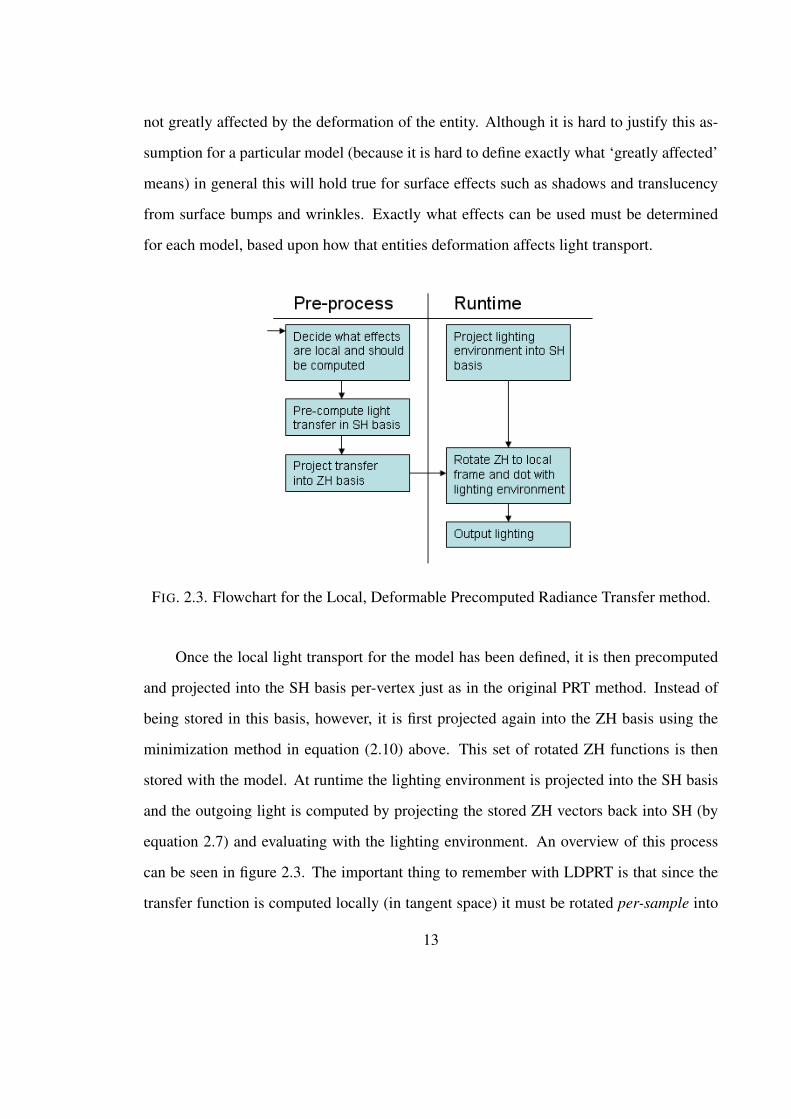
FIG. 2.3. Flowchart for the Local, Deformable Precomputed Radiance Transfer method.
Once the local light transport for the model has been defined, it is then precomputed
and projected into the SH basis per-vertex just as in the original PRT method. Instead of
being stored in this basis, however, it is first projected again into the ZH basis using the
minimization method in equation (2.10) above. This set of rotated ZH functions is then
stored with the model. At runtime the lighting environment is projected into the SH basis
and the outgoing light is computed by projecting the stored ZH vectors back into SH (by
equation 2.7) and evaluating with the lighting environment. An overview of this process
can be seen in figure 2.3. The important thing to remember with LDPRT is that since the
transfer function is computed locally (in tangent space) it must be rotated per-sample into
13

the global space before evaluation. Although SH rotation is feasable to perform per-frame,
it is too expensive to compute per-sample for each frame. ZH rotation is much faster, which
is why LDPRT uses a ZH representation of the light transfer function.
It is worth mentioning why LDPRT is useful when it must be used in such a restrictive
environment. Although it is true that LDPRT doesn’t work with global illumination effects,
which is touted as the main advantage of the original PRT method, it does eliminate the
most inconvenient of the original PRT restrictions: realtime deformation. As noted before,
any PRT method will be performing precomputation over some portion of the model, and
that portion must not be deformed (too drastically) at runtime. LDPRT tries to represent
the light transport that is least affected by deformation, and thus not be as restrictive on the
mesh.
14

Chapter 3
METHOD
Since the principal type of illumination that we are trying to capture is microgeometric
self-shadowing, we use the LDPRT process with a single volume of fur. This volume,
which we store and render with a multiple-shells technique, is constructed by sampling our
target geometry using a simple three-dimensional box filter.
Our method is to combine the successful real-time fur rendering of Lengyel et al
[2001] with LDPRT lighting. Our approach can be summarized as follows:
1. Create a realistic volumetric fur model
2. Precompute illumination of the fur volume
3. Render the volume
4. Reconstruct the lighting
3.1 Creating a realistic volumetric fur model
Several things are necessary to create a good fur model. First, hairs need to start out
thick and become thinner as they go out. We model this by choosing a random width for the
base of each hair and calculating a linear falloff as the hair goes upward. Second, they need
to curl. We model this with a simple parabolic trajectory in a random direction. Third, the
15

textures generated should be antialiased. This is important to prevent jaggies from making
individual hairs appear to jump around as they go up. Our approach approximates a simple
box filter for each voxel that the hair goes through. This is done by slicing the voxel with
several horizontal planes. The area of the hair that intersects each plane is then calculated,
and the results averaged together.
In order to simplify this calculation, we restrict the width of hairs to be at most 1 pixel,
limiting the number of adjacent pixels that a hair can intersect to four. With these restric-
tions, the generation of each hair can be reduced into the cases where the hair intersects
exactly 1, 2, 3 or 4 pixels on each level. These cases can be computed relatively easily with
the basic formulas for the area of circles, wedges, and chords.
FIG. 3.1. Left: Closeup of several hairs. Center: Top-down view of fur volume with colorset by depth. Right: Final rendering of fur volume.
The last major feature that we address is the number and type of the hairs that we
model. Both Kajiya [1989] and Gelder [1997] note the importance of including two layers
of fur in their models. The undercoat is made of short hairs that form a dense layer around
the object, while the overcoat is composed of longer, thicker hairs. Our approach renders
both of these layers by changing the range of widths that each hair starts with. The under-
coat will start with a very small width, and will peter out quickly as it goes upward. Longer
hairs start with a thicker base and will reach a much greater distance from the base before
16
thinning out. Figure 3.1 shows several views of our fur volume.
3.2 Precomputing illumination of the fur volume
Our lighting method is based upon the lighting model for hair described developed by
Kajiya et al [1989]. Their method was composed of 1) calculating the attenuation of scene
lighting to each voxel on a fur volume, 2) modeling the microgeometry of fur through a
lighting model, and 3) calculating the attenuation of the light from the surface to the eye.
Our current method only does step 1, which effectivly means that we are calculating the
sum illuminance to each point in the volume. We are currently only computing light atten-
uation in the volume, and not taking into account scattering. The addition of a scattering
term could potentially increase the realism of the fur significantly. Step 2 in their method
converts the illuminance value into sum luminous exitance, a step which we push back
from the precomputation to the reconstruction. This gives us the ability to use heteroge-
neous lighting models that vary over position and/or time. Our current implementation,
however, doesn’t take advantage of this freedom and simply displays the light reaching
each voxel without any further computation. We perform Step 3 of their method at runtime
through alpha blending on graphics hardware. Note that our use of the radiometric terms
illuminance and luminous exitance are based upon calculation summed across the entire
surrounding sphere to each point, and not just the hemisphere above.
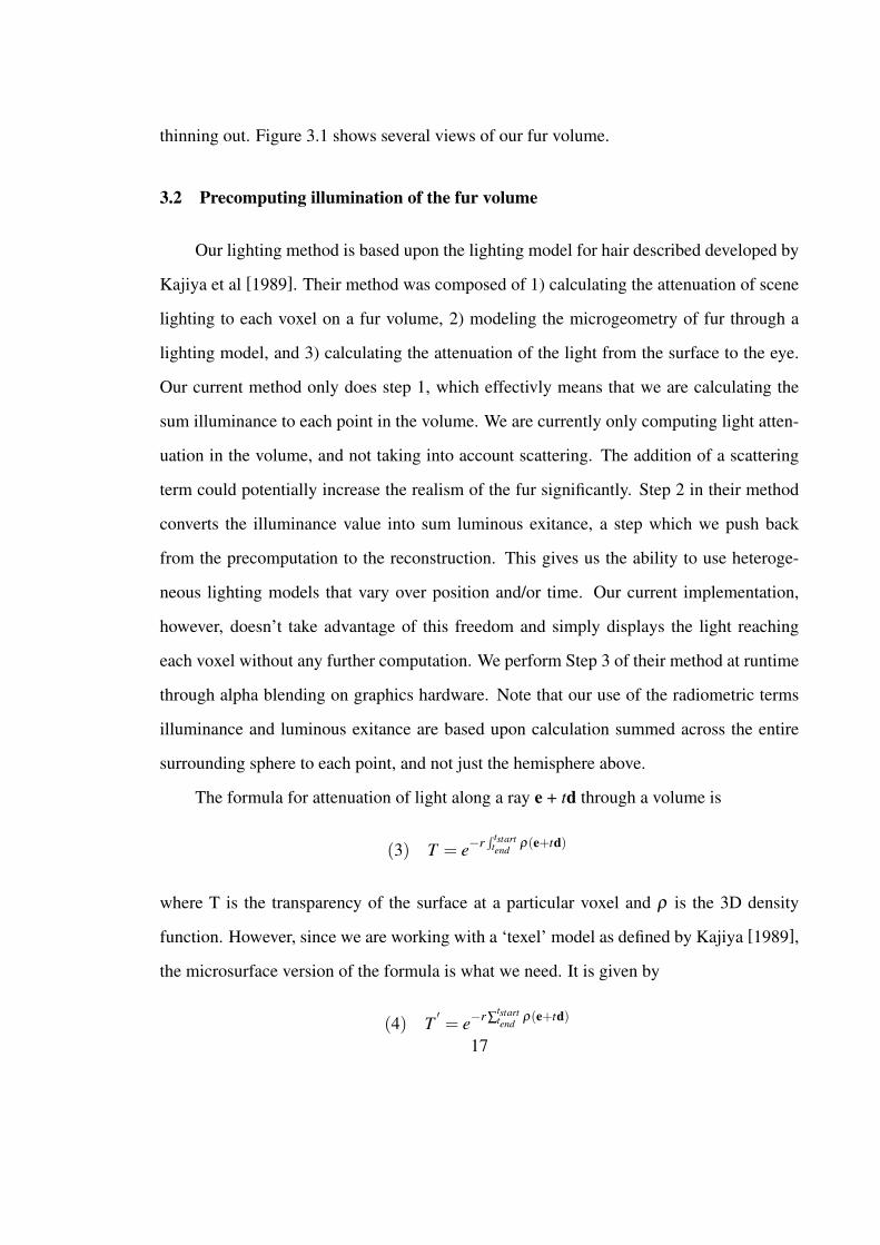
The formula for attenuation of light along a ray e + td through a volume is
(3) T = e−r∫ tstart
tendρ(e+td)
where T is the transparency of the surface at a particular voxel and ρ is the 3D density
function. However, since we are working with a ‘texel’ model as defined by Kajiya [1989],
the microsurface version of the formula is what we need. It is given by
(4) T′= e−r ∑tstart
tendρ(e+td)
17
This version is exactly the same as (3.2) except the integral is replaced with a sum to
take into account the fact that line integrals through surfaces go to zero, which is not what
we want. Instead, we sum the contribution of each surface along the ray. Our implemen-
tation of this lighting calculation takes the the vector d and the ‘texel’ volume data and
marches a ray from the center of each voxel in the direction of d until it leaves the volume,
adding the density of each voxel hit scaled by the length of ray that passed through it. Note
that this is in effect placing the light at infinity in the direction defined by the vector d.
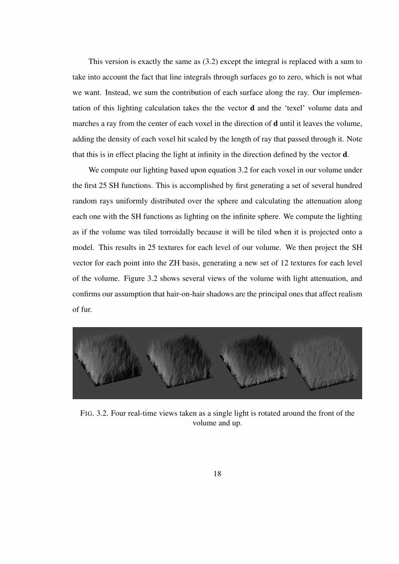
We compute our lighting based upon equation 3.2 for each voxel in our volume under
the first 25 SH functions. This is accomplished by first generating a set of several hundred
random rays uniformly distributed over the sphere and calculating the attenuation along
each one with the SH functions as lighting on the infinite sphere. We compute the lighting
as if the volume was tiled torroidally because it will be tiled when it is projected onto a
model. This results in 25 textures for each level of our volume. We then project the SH
vector for each point into the ZH basis, generating a new set of 12 textures for each level
of the volume. Figure 3.2 shows several views of the volume with light attenuation, and
confirms our assumption that hair-on-hair shadows are the principal ones that affect realism
of fur.
FIG. 3.2. Four real-time views taken as a single light is rotated around the front of thevolume and up.
18

3.3 Rendering the volume
The next step is to render the volume onto a model in realtime. We use the shell/fin
method described by Lengyel [2001]with a few changes. His method described generating
concentric shells around a model and rendering each shell with an alpha-blended texture
that is generated by sampling that level shell from the fur volume, which corresponds to
that level in the volume. This works very well for giving the impression of geometric
fur because the offset between shells gives the correct movement of hairs relative to the
camera. However, around the silhouette of the object the shells become parallel to the
view direction, which makes the gaps between the shells apparent. To remedy this Lengyel
adds fins, which are quads that stand perpendicular to the model generated by extruding
the edges outward. These shells are also sampled into the fur volume, vertically instead of
horizontally, to reflect their orientation to the model.
Lengyel noted that the stochastic property of fur hides certain boundaries and used
this fact several times to his advantage. We cannot make this assumption, however, because
the precomputed lighting requires that the hair neighborhoods remain constant through the
rendering stage. Lengyel uses his observation first when he uses Lapped Textures [Praun et
al., 2000] to paste the fur volume on the model. We cannot do this, so we simply torroidally
tile the volume across the model. This means that we must be careful when generating the
volume and precomputing the lighting that no seams appear on the boundary, and that we
must rely on the UV mapping to minimize distortion to ensure smooth fur without local
distortions. Although Lengyel noted that the correct way to generate the textures for the
fins was to sample the volume, he took advantage of the stochastic nature of fur a second
time to blend new textures generated to appear like the fur volume on the model. Again, we
cannot make this assumption and must sample our fins directly from the fur volume. For
this reason, we have not yet added fins into our model. Figure 3.2 shows several screens of
our method being rendered on a simple plane.
19

Our implementation of the concentric shells technique uses a vertex shader to perturb
the vertices of the model [Isidoro and Mitchell, 2002]. We draw the model once for each
shell needed, perturbing the vertices along the normal a different amount each time in a
linear fashon. We found that 16 shells was usually sufficient to create realistic fur.
3.4 Reconstructing the lighting
The final stage in our method is reconstruction of lighting in realtime. Because we
have the precomputed PRT values in the ZH bases, we can rotate them to match our local
frame for each point on the surface and project back into the SH basis. The lighting envi-
ronment is then projected into the SH basis and the dot product between the transfer and
the lighting is computed, resulting in the final lighting of the point.
Because we precomputed transfer in a set of textures, the rotation of the transfer func-
tion to the local frame, conversion into SH, and the final dot product must be done per pixel.
We perform these calculations in a pixel shader, passing the interpolated normal to define
the local frame in through a vertex shader. All of our PRT coefficients for the transfer
function are stored in textures and evaluated on graphics hardware.
The actual rotation of the ZH functions is a problem that we have not yet completely
solved. Even though rotation on graphics hardware is efficiently performed using homo-
geneous rotations matrices, our use of textures to store ZH coefficients (including the ZH
rotation) means that storing 4x4 matrices is simply too costly in memory compared to other
representations of a rotation. The three alternative representations we considered were po-
lar coordinates, unit length vectors (points on the unit sphere), and quaternions. Polar
coordinates are useful because they can describe a rotation with only two coefficients, the
drop angle and the rotation angle. This allows us to store our spherical functions into two-
dimensional textures for easy access, as well as store our actual rotation using only two
coefficients. However, we found that they were not appropriate for performing the actual
20

rotation on graphics hardware because of visual artifacts introduced near when the drop an-
gle equaled 0 or π (which are the poles on the unit sphere). We are currently investigating
the use of unit vectors and/or quaternions to perform this rotation efficiently on graphics
hardware.
21

Chapter 4
RESULTS
We performed our work on two separate machines: An Athlon 64 3000+ machine
with 2 Gigabytes of ram and a Nvidia 6800 video card, and a dual processor Pentium 4
3.2 GHz machine with 2 Gigabytes of ram and an ATI X1800 video card. All tests were
performed at 1024x768 resolution. The Nvidia machine achieved 20-25 FPS, while the ATI
machine achieved 30-40 FPS. It is our opinion that the difference in speed here is not due to
any fundamental difference in the hardware, but to the fact that the ATI card is somewhat
newer and contains more pixel shader engines. We believe that these results allow us to
claim real-time performance for our method.
Even though we are performing a very complicated technique that requires a lot of
different textures, the stochastic nature of fur allows us to use very small texture sizes, and
so they do not consume very much memory on graphics hardware. Refer to figure 4.1 for
a complete list of textures used in our implementation. Note that the textures containing
geometry and transfer function information must be stored per-shell, while only one set of
SH lookup textures are needed for the entire set. Our method only takes 256 Kb of texture
space in total, although this will vary depending on the desired physical characteristics of
the microgeometric volume. Changing the size of the volume and transfer function textures
allows for more detailed or larger microgeometry tiles.
It is worth noting that the bottleneck for our method is pixel shader performance. This
22

is because we perform the rotation and projection from ZH to SH of the transfer function in
the pixel shader, and this calculation is longer than any other stage in the graphics pipeline.
However, this problem is not unique to our method, since pixel shader engines have always
been in higher demand that vertex shader engines. This is partly because pixel shaders have
to be run for each pixel on the screen while vertex shaders are only run on the vertices of a
model, but we believe that it is also caused by the increased burden that advanced shading
methods, such as ours, put on the pixel shader. We expect our method to be practical on the
latest generation of hardware that has already been released, including the Nvidia 7900 and
ATI X1900 series, because they have a much higher pixel/vertex shader ratio. Preliminary
results have shown these cards might even double the speed of our method.
FIG. 4.1. Table showing the different textures needed, along with their sizes and the totalsize. In an actual implementation these textures would be packed into a set of 4-channeltextures for efficient handling on graphics hardware.
23
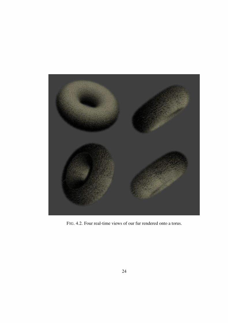
FIG. 4.2. Four real-time views of our fur rendered onto a torus.
24

FIG. 4.3. Four views of the torus as the light is rotated down in front. Note the highlightson the tips of hairs that are at a grazing angle to the light.
25
Chapter 5
CONCLUSIONS AND FUTURE WORK
We have introduced a novel combination of accepted rendering techniques aimed at
rendering complex materials like fur in real-time. Our technique is feasable on current-
generation hardware, and shows that realistic microgeometric surfaces are now within reach
in the stringent real-time rendering environment. Specifically, we have shown that it is
possible to display locally-based global illumination that is necessary for realistic micro-
geometry by producing an example with fur where each hair can cast shadows onto other
hairs.
Several elements of our implementation could be extended to reproduce a more com-
plete version of either PRT or fur rendering. An improved lighting model would make the
fur look much better. Such a model could be based upon the Kajiya [1989] frame bundle
technique, or something else. An interesting approach would be to store this information
and pass it to the shader at runtime, which would allow varying lighting models across the
surface and/or a single set of precomputed lighting maps for different styles of fur. Such a
technique could vastly improve the realistic look of the fur and allow much more flexibility.
[Isidoro and Mitchell, 2002]
Two things that were done by Lengyel et al [2001] that could be modified to work in
our renderer were varying the color of fur over the surface (ours is uniform) and creating
‘fin’ textures to add substance when the shells are nearly parallel with the viewing direction.
26

The dog model in their paper is a good example of the type of effects that color variation
can display, and combined with the realistic lighting model that we present, could go a long
way toward photorealistic fur in real-time. The texture fins are really a necessary part of
a fur shell texture implementation, but our model adds the extra complexity of having to
perform PRT on the fin textures as well as the shell textures.
Lastly, a technique that could increase the flexibility of the rendering could be to sam-
ple the volume onto arbitrary slices at runtime. This technique could allow for view-aligned
slices, thus removing the need for fins altogether. This is logical because our method would
require arbitary sampling for the fins anyway (because the neighborhood of hairs is impor-
tant). In addition, this would allow us to remove some geometry from the model because
of the removal of fins.
27

REFERENCES
[Gelder and Wilhelms, 1997] Allen Van Gelder and Jane Wilhelms. An interactive fur
modeling technique. In Proceedings of Graphics Interface 1997. Graphics Interface,
1997.
[Green, 2003] R. Green. Spherical harmonic lighting: The gritty details. In Proceedings
of GDC, 2003. Game Developers Conference, 2003.
[Isidoro and Mitchell, 2002] John Isidoro and Jason L. Mitchell. User customizable real-
time fur. In SIGGRAPH 2002 Proceedings. ACM, 2002.
[Kajiya and Kay, 1989] James T. Kajiya and Timothy L. Kay. Rendering fur with three
dimensional textures. In ACM SIGGRAPH Computer Graphics Vol. 23, Issue 3. ACM
SIGGRAPH, July 1989.
[Kristensen et al., 2005] Anders Wang Kristensen, Tomas Akenine-Moler, and Hen-
rik Wann Jensen. Precomputed local radiance transfer for real-time lighting design.
In Proceedings of SIGGRAPH 2005. ACM, ACM Press / ACM SIGGRAPH, 2005.
[Lengyel et al., 2001] Jerome Lengyel, Emil Praun, Adam Finkelstein, , and Hugues
Hoppe. Real-time fur over arbitrary surfaces. In Proceedings of the 2001 symposium on
Interactive 3D graphics. ACM, ACM Press / ACM SIGGRAPH, 2001.
[Liu et al., 2004] Xinguo Liu, Peter-Pike Sloan, Heung-Yeung Shum, and John Snyder.
All-frequency precomputed radiance transfer for glossy objects. In Eurographics Sym-
posium on Rendering 2004. The Eurographics Association, The Eurographics Associa-
tion, 2004.
28
[Lokovic and Veach, 2000] Tom Lokovic and Eric Veach. Deep shadow maps. In Pro-
ceedings of SIGGRAPH 2000. ACM, ACM Press / ACM SIGGRAPH, 2000.
[Perlin and Hoffert, 1989] Ken Perlin and Eric M. Hoffert. Hypertexture. In ACM SIG-
GRAPH Computer Graphics Vol. 23, Issue 3. ACM SIGGRAPH, July 1989.
[Praun et al., 2000] Emil Praun, Adam Finkelstein, , and Hugues Hoppe. Lapped textures.
In Proceedings of SIGGRAPH 2000. ACM, ACM Press / ACM SIGGRAPH, 2000.
[Sloan et al., 2002] Peter-Pike Sloan, Jan Kautz, and John Snyder. Precomputed radiance
transfer for real-time rendering in dynamic, low-frequency lighting environemnts. In
Proceedings of SIGGRAPH 2002. ACM, ACM Press / ACM SIGGRAPH, 2002.
[Sloan et al., 2003] Peter-Pike Sloan, Xinguo Liu, Heung-Yeung Shum, and John Snyder.
Bi-scale radiance transfer. In Proceedings of SIGGRAPH 2003. ACM, ACM Press /
ACM SIGGRAPH, 2003.
[Sloan et al., 2005] Peter-Pike Sloan, Ben Luna, and John Snyder. Local, deformable pre-
computed radiance transfer. In Proceedings of SIGGRAPH 2005. ACM, ACM Press /
ACM SIGGRAPH, 2005.
[Wang et al., 2005] Rui Wang, John Tran, and David Luebke. All-frequency interactive
relighting of translucecnt objects with single and multiple scattering. In Proceedings of
SIGGRAPH 2005. ACM, ACM Press / ACM SIGGRAPH, 2005.
29
Top Related