


Languages
Pages
Legal


A TIME DOMAIN STRIP THEORYAPPROACH TO PREDICT MANEUVERING IN
A SEAWAY
by
Rahul Subramanian
A dissertation submitted in partial fulfillmentof the requirements for the degree of
Doctor of Philosophy(Naval Architecture and Marine Engineering)
in The University of Michigan2012
Doctoral Committee:
Professor Robert F. Beck, ChairAssociate Professor Bogdan EpureanuSenior Associate Research Scientist Okey G. NwoguProfessor Armin W. Troesch

ACKNOWLEDGEMENTS
I would like to humbly acknowledge everyone who has directly or indirectly helped
in making this dissertation a success.
First and foremost, I would like to thank my adviser and mentor, Prof. Beck for
giving me the opportunity to work with him. His immense knowledge, experience
and insight in the subject have helped make this dissertation possible. His easy going
nature and friendly personality have made it a pleasure to work with him. His kind
words of encouragement and appreciation have helped me overcome even the most
stressful phases of my research work.
I would like to thank my doctoral committee members, Prof. Troesch, Prof.
Epureanu, and Dr. Nwogu for their helpful suggestions and comments. They have
helped me to obtain new perspectives and insights into the problem.
I would like to express my love and gratitude for my parents Prof. Anantha
Subramanian and Mrs. Prema for all their support and encouragement. My dad
being a naval architect himself, inspired me from my early days to pursue a career
in naval architecture and ocean engineering. A special thanks also goes out to our
family friend Mr. GRP Subramaniam for all his help. A special thanks also goes out
to my sister Gayathri, for all her encouragement and moral support.
A big thanks goes to my dear friends, Johny, Venky, Mahesh, Prasanna, Iyer,
Manu, M Harish, Rajhesh, and Thrushal who not only supported me but also made
my stay in Ann Arbor a memorable one.
I would like to thank Dr. Maki and his research team, in particular William
ii

Rosemurgy and John for helping me set up the OpenFOAM runs in the final stage
of my dissertation work.
I would like to thank my colleagues and staff in the department for all their
technical and administrative support.
The project was partially funded by the Office of Naval Research, award number
N00014-05-1-0537, and their support is greatly acknowledged.
iii

TABLE OF CONTENTS
ACKNOWLEDGEMENTS . . . . . . . . . . . . . . . . . . . . . . . . . . ii
LIST OF FIGURES . . . . . . . . . . . . . . . . . . . . . . . . . . . . . . . vi
LIST OF TABLES . . . . . . . . . . . . . . . . . . . . . . . . . . . . . . . . ix
LIST OF APPENDICES . . . . . . . . . . . . . . . . . . . . . . . . . . . . x
ABSTRACT . . . . . . . . . . . . . . . . . . . . . . . . . . . . . . . . . . . xi
CHAPTER
I. Introduction . . . . . . . . . . . . . . . . . . . . . . . . . . . . . . 1
1.1 Background . . . . . . . . . . . . . . . . . . . . . . . . . . . . 11.2 Overview . . . . . . . . . . . . . . . . . . . . . . . . . . . . . 3
II. Problem Formulation . . . . . . . . . . . . . . . . . . . . . . . . . 5
2.1 Definition Sketch . . . . . . . . . . . . . . . . . . . . . . . . . 52.2 Mathematical Formulation . . . . . . . . . . . . . . . . . . . 72.3 Strip Theory Approximation . . . . . . . . . . . . . . . . . . 112.4 Strip Theory Boundary Value Problem . . . . . . . . . . . . . 122.5 Boundary Integral Method . . . . . . . . . . . . . . . . . . . 152.6 Forces and Moments . . . . . . . . . . . . . . . . . . . . . . . 162.7 Equations of Motion . . . . . . . . . . . . . . . . . . . . . . . 172.8 The Acceleration Potential . . . . . . . . . . . . . . . . . . . 212.9 External Forces . . . . . . . . . . . . . . . . . . . . . . . . . . 24
III. Numerical Techniques . . . . . . . . . . . . . . . . . . . . . . . . 30
3.1 Source Distribution Formulation . . . . . . . . . . . . . . . . 303.2 Domain Discretization . . . . . . . . . . . . . . . . . . . . . . 323.3 Time Integration . . . . . . . . . . . . . . . . . . . . . . . . . 33
iv
3.4 Blending Scheme . . . . . . . . . . . . . . . . . . . . . . . . . 353.5 Radial Basis Functions . . . . . . . . . . . . . . . . . . . . . . 36
IV. Free Motion Drift . . . . . . . . . . . . . . . . . . . . . . . . . . . 39
V. Maneuvering Results . . . . . . . . . . . . . . . . . . . . . . . . . 55
5.1 Calm Water Turning Circle Test . . . . . . . . . . . . . . . . 555.2 Turning Circle Test in Regular Waves . . . . . . . . . . . . . 56
VI. Surge Damping Model . . . . . . . . . . . . . . . . . . . . . . . . 73
6.1 Empirical Scheme . . . . . . . . . . . . . . . . . . . . . . . . 736.2 URANS Formulation . . . . . . . . . . . . . . . . . . . . . . . 746.3 Results and Discussion . . . . . . . . . . . . . . . . . . . . . . 74
VII. Conclusions and Recommendations . . . . . . . . . . . . . . . . 84
APPENDICES . . . . . . . . . . . . . . . . . . . . . . . . . . . . . . . . . . 86A.1 Forced Heave Problem . . . . . . . . . . . . . . . . . . . . . . 87A.2 Free Motion Drift . . . . . . . . . . . . . . . . . . . . . . . . 88B.1 Scale Factor Test . . . . . . . . . . . . . . . . . . . . . . . . . 94B.2 Coordinate Frame Invariance Test . . . . . . . . . . . . . . . 95
BIBLIOGRAPHY . . . . . . . . . . . . . . . . . . . . . . . . . . . . . . . . 101
v

LIST OF FIGURES
Figure
2.1 DEFINITION SKETCH . . . . . . . . . . . . . . . . . . . . . . . . 62.2 OVERHEAD VIEW OF COORDINATE FRAMES . . . . . . . . . 82.3 BODY COORDINATE FRAME . . . . . . . . . . . . . . . . . . . . 183.1 DETAILS AT A GIVEN STATION . . . . . . . . . . . . . . . . . . 344.1 FREE MOTION DRIFT OF WIGLEY-I, λ/L = 1.0, H/λ = 1/50,
WAVE DIRECTION= 45o, NO SWAY-YAW VISCOUS FORCES . 424.2 FREE MOTION DRIFT OF WIGLEY-I, λ/L = 1.0, H/λ = 1/50,
WAVE DIRECTION= 45o, WITH SWAY-YAW VISCOUS FORCES 444.3 FREE MOTION DRIFT OF WIGLEY-I, λ/L = 1.0, H/λ = 1/50,
WAVE DIRECTION = HEAD SEAS, WITH SWAY-YAW VISCOUSFORCES . . . . . . . . . . . . . . . . . . . . . . . . . . . . . . . . . 45
4.4 FREE MOTION DRIFT OF WIGLEY-I, λ/L = 1.0, H/λ = 1/100,WAVE DIRECTION= 45o, WITH SWAY-YAW VISCOUS FORCES 46
4.5 FREE MOTION DRIFT OF WIGLEY-I, λ/L = 0.7, H/λ = 1/50,WAVE DIRECTION= 45o, WITH SWAY-YAW VISCOUS FORCES 47
4.6 FREE MOTION DRIFT OF S-175, λ/L = 1.0, H/λ = 1/50, WAVEDIRECTION= 45o, NO SWAY-YAW VISCOUS FORCES . . . . . 49
4.7 FREE MOTION DRIFT OF S-175, λ/L = 1.0, H/λ = 1/50, WAVEDIRECTION= 45o, WITH SWAY-YAW VISCOUS FORCES . . . . 50
4.8 FREE MOTION DRIFT OF S-175, λ/L = 1.0, H/λ = 1/50, WAVEDIRECTION= 180o, WITH SWAY-YAW VISCOUS FORCES . . . 51
4.9 FREE MOTION DRIFT OF S-175, λ/L = 1.0, H/λ = 1/100, WAVEDIRECTION= 45o, WITH SWAY-YAW VISCOUS FORCES . . . . 52
4.10 FREE MOTION DRIFT OF S-175, λ/L = 1.2, H/λ = 1/60, WAVEDIRECTION= 45o, WITH SWAY-YAW VISCOUS FORCES . . . . 53
4.11 FREE MOTION DRIFT OF S-175, λ/L = 0.7, H/λ = 1/50, WAVEDIRECTION= 45o, WITH SWAY-YAW VISCOUS FORCES . . . . 54
5.1 CALM WATER TURNING CIRCLE OF S-175, δ = −35o . . . . . 575.2 TURNING CIRCLE OF S-175 IN WAVES, δ = −35o, λ/L = 1.0,
HEADING = BEAM SEAS, H/λ = 1/50 . . . . . . . . . . . . . . . 605.3 DETAILS OF ROLL, PITCH AND HEAVE . . . . . . . . . . . . . 61
vi

5.4 TURNING CIRCLE OF S-175 IN WAVES, δ = 35o, λ/L = 1.0,HEADING = BEAM SEAS, H/λ = 1/50 . . . . . . . . . . . . . . . 62
5.5 TURNING CIRCLE OF S-175 IN WAVES, δ = 35o, λ/L = 1.0,HEADING = HEAD SEAS, H/λ = 1/50 . . . . . . . . . . . . . . . 63
5.6 TURNING CIRCLE OF S-175 IN WAVES, δ = −35o, λ/L = 1.0,HEADING = HEAD SEAS, H/λ = 1/50 . . . . . . . . . . . . . . . 64
5.7 TURNING CIRCLE OF S-175 IN WAVES, δ = −35o, λ/L = 1.2,HEADING = HEAD SEAS, H/λ = 1/60 . . . . . . . . . . . . . . . 65
5.8 TURNING CIRCLE OF S-175 IN WAVES, δ = −35o, λ/L = 1.2,HEADING = BEAM SEAS, H/λ = 1/60 . . . . . . . . . . . . . . . 66
5.9 TURNING CIRCLE OF S-175 IN WAVES, δ = 35o, λ/L = 1.2,HEADING = HEAD SEAS, H/λ = 1/60 . . . . . . . . . . . . . . . 67
5.10 TURNING CIRCLE OF S-175 IN WAVES, δ = 35o, λ/L = 1.2,HEADING = BEAM SEAS, H/λ = 1/60 . . . . . . . . . . . . . . . 68
5.11 TURNING CIRCLE OF S-175 IN WAVES, δ = −35o, λ/L = 0.7,HEADING = BEAM SEAS, H/λ = 1/35 . . . . . . . . . . . . . . . 69
5.12 TURNING CIRCLE OF S-175 IN WAVES, δ = 35o, λ/L = 0.7,HEADING = BEAM SEAS, H/λ = 1/35 . . . . . . . . . . . . . . . 70
5.13 TURNING CIRCLE OF S-175 IN WAVES, δ = 35o, λ/L = 0.7,HEADING = BEAM SEAS, H/λ = 1/50 . . . . . . . . . . . . . . . 71
5.14 EFFECT OF INITIAL PHASE ANGLE OF INCIDENT WAVES . 726.1 OpenFOAM COMPUTATIONAL DOMAIN . . . . . . . . . . . . . 786.2 CALM WATER WAVE PATTERN, Fn = 0.30 (OpenFOAM) . . . . 786.3 DYNAMIC PRESSURE ON HULL SURFACE, Fn = 0.30 (Open-
FOAM) . . . . . . . . . . . . . . . . . . . . . . . . . . . . . . . . . 796.4 CALM WATER RESISTANCE, Fn = 0.30 (OpenFOAM) . . . . . . 796.5 SURGE FORCE λ/L = 0.5 . . . . . . . . . . . . . . . . . . . . . . . 806.6 SURGE FORCE λ/L = 1.0 . . . . . . . . . . . . . . . . . . . . . . . 806.7 SURGE FORCE λ/L = 1.5 . . . . . . . . . . . . . . . . . . . . . . . 816.8 SURGE FORCE λ/L = 2.0 . . . . . . . . . . . . . . . . . . . . . . . 816.9 SURGE FORCE λ/L = 2.5 . . . . . . . . . . . . . . . . . . . . . . . 826.10 FREE SURFACE, FORCED SURGE λ/L = 2.5 . . . . . . . . . . . 826.11 COMPARISON OF FORCE AMPLITUDES FROM FFT ANALYSIS 836.12 COMPARISON OF FORCE PHASE FROM FFT ANALYSIS . . . 83A.1 CONVERGENCE STUDIES FOR NUMBER OF BODY PANELS 89A.2 CONVERGENCE STUDIES FOR TIME-STEP SIZE . . . . . . . . 90A.3 CONVERGENCE STUDIES FOR INNER DOMAIN SIZE . . . . . 91A.4 TRACK OF SHIP-CONVERGENCE STUDIES FOR TIME-STEP
SIZE, FREE MOTION DRIFT OF WIGLEY-I . . . . . . . . . . . 92A.5 YAW MOTIONS OF SHIP-CONVERGENCE STUDIES FOR TIME-
STEP SIZE, FREE MOTION DRIFT OF WIGLEY-I . . . . . . . . 93B.1 SCALE FACTOR TEST, WIGLEY-I . . . . . . . . . . . . . . . . . 96B.2 COMPARISON OF TRACK, COORDINATE FRAME INVARIANCE
TEST . . . . . . . . . . . . . . . . . . . . . . . . . . . . . . . . . . 98
vii

B.3 COMPARISON OF YAW MOTIONS, COORDINATE FRAME IN-VARIANCE TEST . . . . . . . . . . . . . . . . . . . . . . . . . . . 99
B.4 COMPARISON OF ROLL AND HEAVE MOTIONS, COORDINATEFRAME INVARIANCE TEST . . . . . . . . . . . . . . . . . . . . . 100
viii

LIST OF TABLES
Table
4.1 HULL PARTICULARS . . . . . . . . . . . . . . . . . . . . . . . . . 415.1 DETAILS OF CONTAINERSHIP S-175 . . . . . . . . . . . . . . . 566.1 DETAILS OF WIGLEY-I HULL . . . . . . . . . . . . . . . . . . . 746.2 TEST MATRIX FOR FORCED SURGE PROBLEM . . . . . . . . 75B.1 WIGLEY-I PARTICULARS FOR SCALE FACTOR TEST . . . . . 95
ix

LIST OF APPENDICES
Appendix
A. Convergence Results . . . . . . . . . . . . . . . . . . . . . . . . . . . . 87
B. Validation of Computer Code . . . . . . . . . . . . . . . . . . . . . . . 94
x

ABSTRACT
A TIME DOMAIN STRIP THEORY APPROACH TO PREDICTMANEUVERING IN A SEAWAY
by
Rahul Subramanian
Chair: Robert F. Beck
A time-domain body exact strip theory is developed to predict maneuvering of a
vessel in a seaway. A frame following the instantaneous position of the ship, by trans-
lating and rotating in the horizontal plane, is used to set up the Boundary Value
Problem (BVP) for the perturbation potentials. Linearized free surface boundary
conditions are used for stability and computational efficiency, and exact body bound-
ary conditions are used to capture nonlinear effects. A nonlinear rigid body equation
of motion solver is coupled to the hydrodynamic model to predict ship responses.
At each time-step, a two-dimensional mixed BVP is solved by using a bound-
ary integral technique. Constant strength panels are used on the body surface and
desingularised sources are placed above the free surface nodes. The constant strength
panels have been shown to have better capability in handling complex hull geome-
tries. The free surface and rigid body equations of motions are evolved in time using
a fourth-order Adams-Bashforth technique. A separate BVP is set up to solve for the
acceleration potential.
xi

Forced oscillation problems are used to study convergence with respect to time-
step size, number of body panels and free surface domain length. The seakeeping
prediction capabilities of the method have been established by Bandyk (2009).
As a first stage of the research, the drifting of a ship freely floating without
power in a seaway is simulated. Simulations are performed with and without viscous
corrections, and give some interesting results. The Wigley-I and the containership
S-175 are used for these studies. This is used to establish the robustness and stability
of the code to perform long time simulations on the order of hundreds of wave periods.
The second stage of the thesis involves the prediction of controlled maneuvers of
the containership S-175 in calm waters and in the presence of waves. The turning
circle maneuver is performed on the S-175, and results compared with available ex-
perimental results. The simulations are able to capture general qualitative aspects
and the essential physics of the problem. Computational issues are addressed in this
chapter.
The third stage of the research involves the formulation of an empirical surge force
model used in the methodology to correct the potential flow results. Comparisons
are made with results obtained from open source CFD solver OpenFOAM.
The methodology has been shown to be robust, computationally efficient, and
capable of predicting long time simulations of a ship maneuvering in a seaway. Al-
though the basic physics of the problem are captured, the research is in a nascent
stage, and computational issues are present. These are addressed wherever possible,
and recommendations suggested. Also better models for external forces such as pro-
peller thrust, rudder lift forces, and viscous modeling are required to improve the
predictions of the method.
xii

CHAPTER I
Introduction
Ship maneuvering and seakeeping have traditionally been dealt with as separate
sub problems. Maneuvering is predicted in calm waters and seakeeping has to do with
the response of the ship in waves. These give very important information to the naval
architect during the initial stages of design. But in reality, they are coupled in nature.
Presence of waves are known to effect course keeping and maneuvering performance
of a ship by way of wave induced drift forces. On the other hand, maintaining a given
course can induce severe ship motions, increase resistance and decrease propulsive
efficiency and speed.
1.1 Background
Mathematical models have been used by several authors to study maneuvering of
ships in a seaway. Hirano et al. (1980) used three-dimensional equations of motion in
calm water to predict maneuvering performance by computing only wave drift forces.
McCreight (1986) developed a maneuvering model in waves, in which the hydrody-
namic forces were evaluated in a body-fixed coordinate system. The hydrodynamic
coefficients were computed by linear strip-theory. Ottosson and Bystrom (1991) used
a more simplified approach, where the hydrodynamic radiation coefficients were as-
sumed to be constant based on mean encounter frequency during maneuvering motion.
1

Fang et al. (2005) developed a mathematical model taking into account the frequency
of encounter into the time-domain simulation.
The models mentioned above do not take into account the memory effect due to
ship motions. One popular approach to do so is the use of linear convolution integrals
of Cummins (1962). Bailey et al. (1997) and Fossen (2005) have developed unified
models for maneuvering in a seaway, using this approach. Recently Skejic and Faltin-
sen (2008) have developed a unified 4-DOF maneuvering model in which the mean 2nd
order wave loads were added using a direct pressure integration scheme. A two time
scale approach was used in their methodology where the high frequency seakeeping
was separated from the low frequency maneuvering problem. Lin et al. (2006) and
Yen et al. (2010) solved the unified problem using a three-dimensional panel method.
Their study was basically an extension of the nonlinear ship motion prediction code
LAMP (Large Amplitude Motion Program). Recently, Seo and Kim (2011) extended
the time-domain motion program WISH (computer program for nonlinear Wave In-
duced load and SHip motion analysis) based on a B-spline Rankine panel method
to couple seakeeping and maneuvering. Second order wave drift forces were com-
puted by direct pressure integration and modular-type maneuvering model (MMG)
is integrated with seakeeping model.
Experimental methods, although an important tool to estimate wave effects on
ship maneuvering, and to validate mathematical models and numerical methods; are
difficult to conduct, very expensive and can suffer from scale effects. Nonetheless, sev-
eral results have been presented using free-running model tests. Hirano et al. (1980)
performed turning circle maneuvers in regular waves. Ueno et al. (2003) have carried
out turning, zig-zag and stopping tests with a VLCC model. Recently, Yasukawa and
Nakayama (2009) performed turning circle tests of the containership S-175 in both
calm water as well as in waves for a variety of incident wave frequencies, amplitudes
and headings.
2

There has been a lot of recent interest in CFD based methods. Although the
increase in modern computational power has made it feasible to solve the viscous flow
problem in the time-domain, as is done in unsteady Reynolds-Averaged Navier-Stokes
(RANS) codes, the computational effort still remains enormous. Simply performing
a one-minute maneuver may take several hundreds of CPU hours to simulate.
1.2 Overview
This dissertation presents the development of a unified model for predicting the
maneuvering of a ship in a seaway by using a time-domain, strip theory approach. A
hydrodynamic frame following the instantaneous position of the ship in the horizontal
plane is used to set up the BVP. This has the advantage that the path and forward
speed of the ship need not be described in advance, rather all 6 degrees of freedom
are determined by solving the equations of motion.
The strip theory approach allows for faster computational times and simplified
body geometry definition. The use of a blended method ensures that vital nonlinear-
ities are captured while keeping the computational time down.
The theory, numerical methods, results, validations and discussion will be de-
scribed in the following chapters.
Chapter II describes the problem formulation. This includes the coordinate frames
used to set up the problem, conventions used, explanation and justification of assump-
tions made, and description of boundary conditions. The coupling of the hydrody-
namic problem to the equations of motion, the acceleration potential formulation,
and modeling of external forces such as propeller thrust, rudder forces, resistance and
viscous forces are described in detail.
Chapter III describes the details of the numerical schemes used, including dis-
cretization techniques, time marching schemes for the free surface evolution and equa-
tions of motion solver, the details of the numerical damping beach, and radial basis
3

functions to obtain x-derivatives.
Chapter IV presents the results of the free motion drift simulation of the contain-
ership S-175, and Wigley-I hull form.
Chapter V presents the results of the turning circle maneuvers of the containership
S-175 in calm water, and in the presence of regular waves. Comparisons are made
with available experimental results.
Chapter VI presents the results for the surge damping model used to augment the
potential flow results, and comparison with CFD simulations.
Chapter VII summarizes the dissertation work, and discusses the computational
issues present, recommendations and considerations for future work.
4

CHAPTER II
Problem Formulation
2.1 Definition Sketch
The problem definition is as shown in Figure 2.1 where a freely floating rigid body
such as a ship is moving either in calm water or in the presence of external waves. The
objective is to predict the hydrodynamic forces acting on the ship and the resultant
motions and trajectory of such a body.
Three different coordinate systems are used for solving the problem; an earth fixed
inertial axis (xe, ye, ze) is used to keep track of the position of the centre of gravity
of the ship and the Euler angles. A hydrodynamic frame (xh, yh, zh) translates in the
horizontal calm water plane with translational velocities U, V and rotational yaw rate
ψ. It thus follows the ship such that its origin Oh is always in vertical line with the
origin of the body frame, Ob. This is the frame in which the boundary value problem
is formulated in. A body fixed frame (xb, yb, zb) rotates and translates in all 6-DOF
with the body. The frame is used to compute the forces acting on the ship and to
solve for the equations of motions.
The velocities U, V and ψ are the instantaneous body velocities resolved in the
hydrodynamic frame.
5

xh
z b
yb
z e
xb
Oh
Ob
Wav
es c
reat
ed d
ue
to s
hip
Ear
th f
ixed
fra
me
V
Body f
ram
e
Hydro
dynam
ic f
ram
e
U
Inci
den
t w
aves
z h
yh
ye
Oh
xe
ψ
Fig
ure
2.1:
SC
HE
MA
TIC
SH
OW
ING
DIF
FE
RE
NT
CO
OR
DIN
AT
EF
RA
ME
SU
SE
D
6
2.2 Mathematical Formulation
Basic Assumptions
The fluid flow problem in marine hydrodynamics is complicated and challenging.
In order to account for viscous effects like wakes, boundary layers, flow separation
and turbulence, there has been a tendency towards the development of numerical
methods based on the Navier-Stokes equations. But even with the increase in modern
computational power, the computer time needed to compute even a few minutes of
real-time simulation remains large and requires enormous amounts of computational
resources. Furthermore, reliable turbulence models are still an area of active research.
Fortunately, the physical model can be simplified considerably without losing its
overall validity. The flow conditions can be assumed such that (i) the fluid is homo-
geneous and incompressible (small Mach number), (ii) the fluid is inviscid, and (iii)
the flow is free of vorticity at t = 0. For an inviscid flow this would imply that the
flow remains irrotational. Combining these assumptions leads to an incompressible,
inviscid and irrotational fluid flow formulation, namely the potential flow model.
Governing Equations
The generalized three-dimensional potential flow problem can be formulated in
terms of a velocity potential φ, representing the perturbation potential for the absolute
fluid velocity. The velocity vector ~v can be written as:
v = ∇φ (2.1)
From Equation (2.1), the continuity equation for the conservation of mass of the fluid
reduces to the Laplace’s equation
∇2φ = 0 (2.2)
7

The relationship between the coordinates (xe, ye, ze) in the earth fixed frame and
the coordinates (xh, yh, zh) in the hydrodynamic frame are given by:
xe = xh cosψ(t)− yh sinψ(t) + I (2.3)
ye = xh sinψ(t) + yh cosψ(t) + J (2.4)
where
I =
t∫(U(τ) cosψ(τ)− V (τ) sinψ(τ))dτ (2.5)
J =
t∫(U(τ) sinψ(τ) + V (τ) cosψ(τ))dτ (2.6)
I and J are the x and y coordinates of the origin of the hydrodynamic frame with
respect to the earth fixed frame as shown in Figure 2.2.
ψ
xh
xe
ye
U
V
Earth fixed frame
Hydrodynamic frame
yh
ship
re
rh
I
J
Figure 2.2: OVERHEAD VIEW OF COORDINATE FRAMES
Here,
8

U(τ), V (τ) = translational velocities of the hydrodynamic frame resolved in the hy-
drodynamic frame.
τ = a dummy variable for integration representing time.
ψ = the heading angle of the hydrodynamic frame with respect to the earth fixed
frame.
From the above equations, the relationship between the time derivative in the
hydrodynamic and earth fixed frame is:
∂
∂t
∣∣∣∣e
=∂
∂t
∣∣∣∣h
− (U · ∇)− (Ψ× rh) · ∇ (2.7)
∂∂t
∣∣e
denotes the temporal derivative with respect to the earth fixed frame
∂∂t
∣∣h
denotes the temporal derivative with respect to the hydrodynamic frame
U is the translational velocity vector of the hydrodynamic frame resolved in the
hydrodynamic frame and given by (U, V, 0)
Ψ is the rotational rate of the hydrodynamic frame given by (0, 0, ψ)
~re and ~rh are the position vector of a point in the earth fixed and hydrodynamic
frame, respectively.
Using the relation in Equation (2.7), the Euler equations representing the mo-
mentum conservation equations reduce to the unsteady Bernoulli equation in the
translating and rotating hydrodynamic frame:
p
ρ+∂φ
∂t−U · ∇φ− (Ψ× rh) · ∇φ+
1
2∇φ · ∇φ+ gz = c(t) (2.8)
Here ∂φ∂t
represents the temporal derivative of the potential taken with respect to the
hydrodynamic frame.
Alternatively, the pressure can also be written with respect to the earth fixed
9

frame
p
ρ+∂φ
∂t
∣∣∣∣e
+1
2∇φ · ∇φ+ gz = c(t) (2.9)
where ∂φ∂t
∣∣e
represents the temporal derivative of the perturbation potential with
respect to the earth fixed frame.
Boundary Conditions
The boundary conditions on the free surface are the linearized kinematic and
dynamic free surface boundary conditions, which follow from the fact that a fluid
particle remains on the free surface and that the pressure is constant everywhere on
the actual free surface respectively. These are derived in the hydrodynamic frame.
The linearized kinematic free surface boundary condition
∂η
∂t=∂φ
∂z+ (U + Ψ× rh) · ∇η on z = 0 (2.10)
and the linearized dynamic free surface boundary condition
∂φ
∂t= −gη + (U + Ψ× rh) · ∇φ on z = 0 (2.11)
Here, η represents the free surface wave elevation which is measured from the calm
water surface.
The body boundary condition is that of non-penetration of the fluid, which trans-
lates to no normal flow through the body surface
∇φ · n = v · n on SB(t) (2.12)
where φ is the total perturbation potential, v is the absolute velocity of a node on
the body surface with respect to the earth fixed frame including velocities due to
10
rotational effects; n is the unit normal vector positive out of the fluid (or into the
body), and SB(t) is the exact wetted body surface.
The boundary conditions at∞ will be discussed in detail in the following sections
where the two-dimensional strip theory boundary value problem is described.
2.3 Strip Theory Approximation
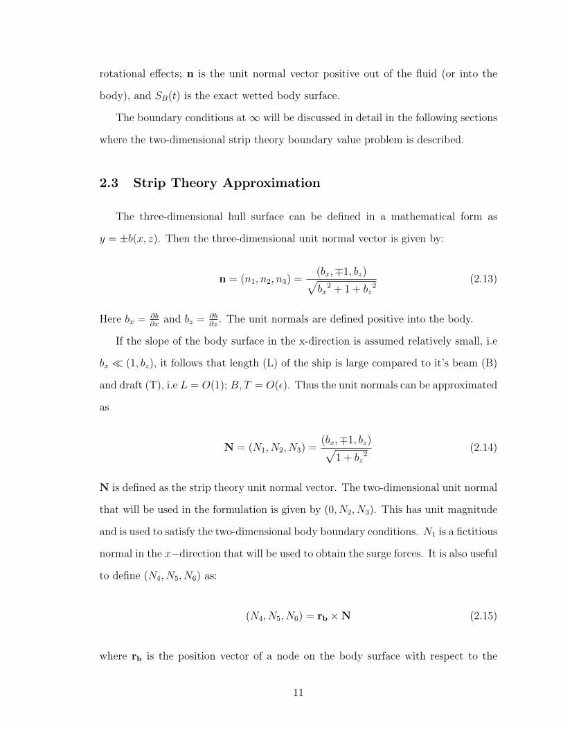
The three-dimensional hull surface can be defined in a mathematical form as
y = ±b(x, z). Then the three-dimensional unit normal vector is given by:
n = (n1, n2, n3) =(bx,∓1, bz)√bx
2 + 1 + bz2
(2.13)
Here bx = ∂b∂x
and bz = ∂b∂z
. The unit normals are defined positive into the body.
If the slope of the body surface in the x-direction is assumed relatively small, i.e
bx � (1, bz), it follows that length (L) of the ship is large compared to it’s beam (B)
and draft (T), i.e L = O(1); B, T = O(ε). Thus the unit normals can be approximated
as
N = (N1, N2, N3) =(bx,∓1, bz)√
1 + bz2
(2.14)
N is defined as the strip theory unit normal vector. The two-dimensional unit normal
that will be used in the formulation is given by (0, N2, N3). This has unit magnitude
and is used to satisfy the two-dimensional body boundary conditions. N1 is a fictitious
normal in the x−direction that will be used to obtain the surge forces. It is also useful
to define (N4, N5, N6) as:
(N4, N5, N6) = rb ×N (2.15)
where rb is the position vector of a node on the body surface with respect to the
11

body fixed frame. Now, the slender-body approximation is used to reduce the three-
dimensional problem into a series of two-dimensional problems at each station or
section of the ship. The detailed boundary value problem is explained in the next
section.
2.4 Strip Theory Boundary Value Problem
Based on the assumptions stated in Section 2.3, the three-dimensional BVP in
Section 2.2 gets reduced to the following two-dimensional BVP:
∇2φ(y, z, t;x) = 0 (2.16)
Here φ = φ(y, z, t;x) shall henceforth refer to the two-dimensional potential for no-
tational convenience.
The free surface boundary conditions take the following form from Equations
(2.10) and (2.11):
∂η
∂t=∂φ
∂z+ V
∂η
∂y+ xhψ
∂η
∂yon z = 0 (2.17)
∂φ
∂t= −gη + V
∂φ
∂y+ xhψ
∂φ
∂yon z = 0 (2.18)
Consistent with strip theory, the encounter frequency is assumed high such that,
∂∂t� U ∂
∂xand the downstream free surface effects are ignored.
In the far field, a radiation boundary condition is imposed such that only the
incident waves are incoming. This is done numerically by incorporating an outer
damping beach and modifying the free surface boundary conditions. The details for
this would be explained in the next Chapter dealing with numerical schemes. All
simulations are carried out in deep water and so the gradient of the perturbation
potential vanishes as z → −∞. This is automatically taken care of by the selection
12

of the Green function, which will be shown in the following section.
Velocity Potential Decomposition and Body Boundary Conditions
The perturbation potentials can be broken down into different components for
proper bookkeeping:
φ(y, z, t;x) = φI + φD + φR
where,
φI = incident wave potential
φD = diffracted potential
φR = radiated potential
The incident wave potential and elevation are known at all time and the linear Airy
wave theory is used. The analytical expressions for the potential and wave elevation
with respect to the earth fixed inertial frame are:
φI =iga
ω0
e−ik(xe cosβ+ye sinβ)eiω0tekz (2.19)
ηI = ae−ik(xe cosβ+ye sinβ)eiω0t (2.20)
13

Here,
a = wave amplitude
ω0 = absolute wave frequency
k = wave number, given by 2π/λ
λ = wavelength
β = heading angle with respect to the earth fixed x-axis
The body boundary condition (2.12) is re-written in terms of it’s individual com-
ponents in the two-dimensional frame
∇φD ·N = −∇φI ·N on SB(t) (2.21)
∇φR ·N = v ·N on SB(t) (2.22)
Here the two-dimensional strip theory normal N discussed in Section 2.3 is used.
SB(t) is the instantaneous wetted body surface. The details of the blending scheme
are given in Section 3.4.
The velocity v used in Equation (2.22) is the velocity of a node on the body
surface with respect to the earth fixed frame and includes all the three translational
and rotational components, namely (u, v, w, p, q, r). Since this is a strip theory for-
mulation, care has to be taken not to include the steady forward speed component
of the velocity into the body boundary condition, as this represents a steady flux of
fluid into the two-dimensional domain and can cause continuity issues. In any case,
solving the steady forward speed problem in a strip-theory formulation is of little use.
In order to circumvent this problem, the following procedure is used. The velocity v
can be assumed to consist of a time-varying mean component v(t), and an oscillatory
14

component v(t), such that
v = v(t) + v(t) (2.23)
The mean component is computed at every time-step by taking the average of the
body velocities over the last number of time-steps
v(t) =
∑i−N+1j=i−1 v(tj)
Tinterval(2.24)
where i is the current time level, j is the counter variable, Tinterval is the length of the
interval for averaging, and N is the number of time-steps in the interval. Tinterval is
chosen as the period of the incident waves. It is important to note that the averaging
is done only in the x-direction, and other degrees are untouched and the velocities
are fully solved for.
The modified body boundary condition is as follows
∇φR ·N = (v −U avg) ·N on SB(t) (2.25)
whereU avg is the mean surge component that is not solved for and given by (u, 0, 0, 0, 0, 0)T .
2.5 Boundary Integral Method
To solve for the two-dimensional problem, Green’s theorem is used with respect to
the potential to write the fluid flow problem as a set of boundary integral equations.
The source distribution method is used in this formulation and the perturbation
potential is given by:
φ(x) =
∫C
σ(ξ)G(x; ξ)dC (2.26)
15

where,
C = contour defining the perimeter of the 2-D boundary,
x = point anywhere in the fluid domain,
ξ = position of source points on boundary C,
σ = unknown source strength,
G = Green function satisfying Laplace’s equation
The two-dimensional Rankine source Green function used is
G(x; ξ) = ln |x− ξ| (2.27)
and has the following attributes
∇2G = 2πδ(x− ξ) (2.28)
∇G→ 0 as x→∞ (2.29)
where δ is the Dirac delta function. The source strengths are determined such that
they satisfy the boundary conditions. Once they are determined, the spatial deriva-
tives of the potential can be found directly by using the derivative of Equation (2.26).
2.6 Forces and Moments
The pressure formulation that is used in the current method is the one written
in the earth-fixed frame, given by Equation (2.9). The pressure is integrated on the
exact body surface to obtain the forces and moments acting on the ship. The sectional
forces and moments are first obtained and then the pressure is integrated along the
16

length of the vessel.
p
ρ+∂φ
∂t
∣∣∣∣e
+1
2∇φ · ∇φ+ gz = 0 (2.30)
F =
∫L
dx
∫CH
pNdl (2.31)
M =
∫L
dx
∫CH
pr×Ndl (2.32)
Like the potential, the pressure is segregated into different components.
To avoid numerical differencing, a separate BVP is set up for the term ∂φ∂t
known
as the acceleration potential formulation. The advantage is it uses the same influence
matrix as that of the φ problem. The other advantage is that it is stable and not
sensitive to the time-step size when computing the pressure on the body, since ∂φ∂t
is
solved for directly. The details will be explained in the next chapter.
2.7 Equations of Motion
Once the potentials, pressure on the hull and forces and moments acting on the
body are determined, using the position and velocity of the body, the equations of
motion (EOM) are set up. The formulation here basically uses the convention followed
by Fossen (1994).
The forces and moments on the ship are described in the body frame, and the
equations of motion will be solved in the body frame. The origin of the body frame
Ob is set at midships and is such that at t = 0, it is at the calm water line. The EOM
17

Figure 2.3: BODY COORDINATE SYSTEM SHOWING SIGN CONVENTIONSAND DEFINITIONS OF THE 6-DOF (ILLUSTRATION FROM johnclarkeon-line.com)
can be written in compact vector form about Ob as follows:
m[vb + ω × rg + ω × vb + ω × (ω × rg)] +m1∗vb +m2
∗ω = F (2.33)
Ibω + ω × Ibω +mrg × (vb + ω × vb) +m3∗vb +m4
∗ω = M (2.34)
18

where,
m = mass of the ship
vb = [u, v, w]T = linear velocity of body in body frame
ω = [p, q, r]T = angular velocity of body in body frame
rg = [xg, yg, zg]T = position vector of CG with respect to Ob
F = [X, Y, Z]T = force through Ob in body frame
M = [K,M,N ]T = moment about Ob in body frame
Ib =
Ix −Ixy −Ixz
−Iyx Iy −Iyz
−Izx −Izy Iz
= generalised moment of inertia matrix
m∗(t) =
m1∗3×3 m2
∗3×3
m3∗3×3 m4
∗3×3
= generalised radiation impulsive added mass matrix
The generalised radiation impulsive added mass matrix, m∗(t) represents one part
of the solution of the radiation acceleration potential formulation. The details are
given in Section 2.8. The generalised force vector can be described by z = (F,M).
This can be written out in terms of the different components:
z = zFK+zDIFF +zRAD+zS+zHS+zV ISC+zPROP +zCALM+zRUDDER (2.35)
19

where,
zFK = exact Froude-Krylov incident wave force
zDIFF = diffracted wave force
zRAD = radiated wave memory force
zS = force due to ∇φ · ∇φ term in the pressure equation
zHS = exact hydrostatic force
zV ISC = empirical viscous forces in roll, sway and yaw DOF
zPROP = propellor thrust force
zCALM = calm water resistance
zRUDDER = rudder force
The vessel’s position and orientation are described with respect to the earth fixed
coordinates by three translations and rotations, given by ξ.
ξ = [ξ1, ξ2, ξ3, φ, θ, ψ]T (2.36)
Here, {ξ1, ξ2, ξ3} represents the three translations and {φ, θ, ψ} represents the three
Euler angles in roll, pitch and yaw respectively. The velocities in the earth fixed frame
are obtained from the body velocities by use of transformation matrix.
ξ = [T ]v (2.37)
T =
T1 03×3
03×3 T2
20

T1 =
cos θ cosψ sinφ sin θ cosψ − cosφ sinψ cosφ sin θ cosψ + sinφ sinψ
cos θ sinψ sinφ sin θ sinψ + cosφ cosψ cosφ sin θ sinψ − sinφ cosψ
− sin θ sinφ cos θ cosφ cos θ
T2 =
1 sinφ sin θ
cos θcosφ sin θ
cos θ
0 cosφ − sinφ
0 sinφcos θ
cosφcos θ
2.8 The Acceleration Potential
The pressure equation (2.30) requires the evaluation of the temporal derivative
∂φ∂t
. In this methodology, a direct formulation is used to set up a BVP for this term,
called the “acceleration potential”, ϕ.
This method has a number of advantages. Firstly it allows for direct solution
at each time, instead of relying on numerical differencing. It also avoids numerical
difficulties with repanelization techniques. Secondly it can be written in terms of the
body accelerations v. It can therefore be moved to the other side of the rigid body
equations of motion. Overall it improves stability.
The formulation used here is based on the work of Bandyk (2009). Detailed back-
ground study, derivations, validations and comparison with other similar formulations
can be found in Bandyk (2009) and Bandyk and Beck (2011).
The idea is that a BVP can be set up for ϕ in a similar manner as was done
for the velocity potential φ, since the acceleration potential also satisfies the Laplace
equation. A brief derivation of the formulation is as follows. The deep water and far
field boundary conditions are satisfied in the same manner as in the velocity potential
problem. The derivation of the body boundary conditions are involved and require
the application of appropriate time-derivatives in different reference frames. The
21

following time-derivatives with respect to the earth fixed frame are used:
δ
δt
∣∣∣∣e
=∂
∂t
∣∣∣∣e
+ v · ∇ (2.38)
δ
δt
∣∣∣∣b
=∂
∂t
∣∣∣∣b
+ ω× (2.39)
where, the term δδt
∣∣e
is the prescribed rate of change following a body node with
respect to the earth fixed frame and ∂∂t
∣∣e
is the temporal derivative with respect to
the earth fixed frame. The quantity δδt
∣∣b
is the prescribed rate of change of a vector
defined in the body frame following a body node and ∂∂t
∣∣b
is it’s temporal derivative
with respect to the body frame. v is the body node velocity given by vb + ω × rb.
The body boundary conditions for ϕ are derived by taking the time derivative
following a body node, δδt
∣∣e
with respect to the earth fixed frame of the equations
(2.21) and (2.22).
δ
δt
∣∣∣∣e
(∇φD ·N) =δ
δt
∣∣∣∣e
(−∇φI ·N) (2.40)
δ
δt
∣∣∣∣e
(∇φR ·N) =δ
δt
∣∣∣∣e
(v ·N) (2.41)
After applying the chain rule and realizing that ∂N∂t
∣∣b
= 0, the resulting boundary
conditions are
N · ∇ϕDe = N · ∇ϕIe − (ω ×N) · (∇φD +∇φI)−N · [(v · ∇)(∇φD +∇φI)]
(2.42)
N · ∇ϕRe = {vb ·N + (ω × rb) ·N} − (ω ×N) · ∇φR −N · [(v · ∇)(∇φR)]
(2.43)
The above formulations give the body boundary conditions for the acceleration po-
tential ϕe for the diffraction and radiation components with respect to the earth fixed
frame of reference. They can alternatively be derived with respect to the hydrody-
22

namic frame by using Equation (2.7) which relates the time derivative in the two
frames
ϕe = ϕh − U∂φ
∂x− V ∂φ
∂y+ ψ
(yh∂φ
∂x− xh
∂φ
∂y
)(2.44)
The free surface boundary condition is straightforward and follows directly from
the dynamic free surface boundary condition in Equation (2.18) for the φ problem.
By using the relation in Equation (2.44)
ϕe|FS = −gη on z = 0 (2.45)
At this point, since all the potentials and derivatives are solved for, all the quan-
tities on the RHS of equations (2.42) and (2.43) are known with the exception of the
first two terms within the {} of equation (2.43) involving the body accelerations vb
and ω.
The radiation acceleration potential ϕR is split into two components, the impulsive
ϕR, Imp and memory ϕR, Memory, subject to the following boundary conditions
ϕR = ϕR, Imp + ϕR, Memory (2.46)
N · ∇ϕR, Impe = vb ·N + (ω × rb) ·N on SB(t) (2.47)
N · ∇ϕR, Memorye = −(ω ×N) · ∇φR −N · [(v · ∇)(∇φR)] on SB(t) (2.48)
ϕR, Imp = 0 on SFS (2.49)
ϕR, Memory = ϕRe∣∣FS
on SFS (2.50)
The body boundary conditions are applied on the instantaneous wetted body surface,
SB(t). It is observed that the impulsive component is only a function of body accel-
erations and is reduced into six canonical problems. For notational convenience, let
23

χ represent ϕR, Imp. Then χ can be represented as follows
χ =6∑i=1
viχi (2.51)
where vi andχi are the acceleration and scaled acceleration potential, due to a unit
body acceleration, in the ith mode of motion. They are such that they satisfy the
following boundary conditions
N · ∇χi = Ni for (i = 1, ...6) on SB(t) (2.52)
χi = 0 for (i = 1, ...6) on SFS (2.53)
The solution of the χi problem produces the m∗ impulsive added mass matrix seen
in Section 2.7. The components are given by
m∗ij = ρ
∫L
dx
∫SB(t)
χjNidl (2.54)
These terms are then moved to the other side of the equations of motions (2.33) and
(2.34). On the other hand, the solution of ϕR, Memory goes directly into the pressure
equation and is integrated over the entire body to give zRAD, the radiation memory
force in Equation (2.35).
2.9 External Forces
The external forces acting on the body constitute the last four terms in the Equa-
tion (2.35), namely the viscous forces in roll, sway and yaw, propeller thrust force,
calm water resistance and forces from control surfaces such as rudder, fins or thrusters.
24
Viscous Forces
Potential theory does not capture the effects of viscosity. Seakeeping problems are
dominated by inertial effects. However, there are scenarios where viscosity plays a
vital role. This is especially true of vortical flows characterized by separation such as
roll. Crucially, slow motion maneuvering is viscous dominated since potential theory
predicts zero damping force at zero frequency limit.
Additional roll viscous damping is used in this formulation. The model is based
on the empirical corrections made by Himeno (1981). The amount of damping is
a function of the hull form and the section shape, and is usually determined from
experimental results.
The viscous force model used in sway and yaw is based on linear and nonlinear
maneuvering coefficients obtained either from experimental captive model tests such
as Planar Motion Mechanism (PMM) or from empirical formulas from regression
analysis.
The maneuvering coefficients used in Chapter V on the maneuvering of the con-
tainer ship S-175 in calm water and waves are the PMM based derivatives in Son and
Nomoto (1981).
Xvisc = Xvrvr +Xvvv2 +Xrrr
2 surge damping (2.55)
Yvisc = Yvv + Yrr + Yvvvv3 + Yrrrr
3 + Yvvrv2r + Yvrrvr
2 sway damping (2.56)
Nvisc = Nvv +Nrr +Nvvvv3 +Nrrrr
3 +Nvvrv2r +Nvrrvr
2 yaw damping (2.57)
where Xvisc, Yvisc and Nvisc are the viscous damping forces in surge, sway and yaw
respectively. These terms would show up on the right hand side of a typical modular-
type mathematical maneuvering model (MMG model). The forces proportional to
the body accelerations, namely the added mass terms are accounted for by potential
theory. The terms Yvv, Yrr, Nvv and Nrr are related to wave damping and hull lifting
25

forces. The strip theory formulation gives zero wave damping because the waves are
too short to be resolved at slow speeds, but as will be discussed in Chapter V, it does
predict a lift and moment. The lift and moments are already accounted for in the
values of Yj, Nj(j = 2, 6) used in Equations (2.56) and (2.57). This implies that they
are being “double counted”. A detailed analysis of this phenomenon and solution of
this problem is currently outside the scope of the work, but related work can be found
in Yen et al. (2010) and Seo and Kim (2011).
Alternatively, an empirical method can be used to obtain the values of the linear
maneuvering derivatives. In Chapter IV, where the free motion drift simulations
of the containership S-175 and Wigley-I hull form in waves are presented, a semi-
empirical method proposed by Clarke et al. (1983) is used. The hull is assumed to be
a low aspect ratio wing and the maneuvering coefficients are a function of the length
to draft ratio of the ship. The non-dimensional coefficients are given by the following
empirical formulas
Y′
v = −π(T
L
)2(1.0 + 0.4CB
B
T
)(2.58)
Y′
r = −π(T
L
)2(−0.5 + 2.2
B
L− 0.08
B
T
)(2.59)
N′
v = −π(T
L
)2(0.5 + 2.4CB
T
L
)(2.60)
N′
r = −π(T
L
)2(0.25 + 0.039
B
T− 0.56
B
L
)(2.61)
where L,B, T, CB are the length, beam, draft and the block coefficient of the hull.
26

The dimensional values are given by
Yv = Y′
v0.5ρL2Unet (2.62)
Yr = Y′
r 0.5ρL3Unet (2.63)
Nv = N′
v0.5ρL3Unet (2.64)
Nr = N′
r0.5ρL4Unet (2.65)
where ρ is the fluid density and Unet =√u2 + v2 is the net speed of the ship.
The rest of the terms in Equations (2.55)-(2.57) are nonlinear viscous damping
terms. They contribute significantly when the low frequency yaw rates and sway
velocities are high such as in a tight turning circle maneuver.
Propeller Thrust Force
The thrust model used in the current method is the one presented in Son and
Nomoto (1981). The thrust force is given by
Tprop = (1− t)ρn2D4KT (2.66)
where Tprop, t, n, D and KT are the propeller thrust force, the thrust-deduction
fraction, propeller revolutions per second, propeller diameter, and thrust coefficient,
respectively. The thrust coefficient, KT is expressed as a linear function of the advance
ratio, J
KT = 0.527− 0.455J (2.67)
J = u′PUnet/nD (2.68)
27

where u′P represents the effective wake fraction given by
u′P = cos v′[(1− wp) + τ(v′ + x′pr′)2] (2.69)
where wp is the wake fraction in straight-ahead condition, v′ and r′ are the non-
dimensional sway and yaw velocities, x′p is the x-location of the propeller plane, and
τ is a parameter to account for the lateral velocity components.
Calm water Resistance
The calm water resistance is estimated according to the quadratic curve fit for
low Froude numbers, given in Son and Nomoto (1981)
X(u) = X ′u|u|0.5ρL2u|u| (2.70)
where X ′u|u| is the total calm water resistance coefficient at model scale set at a con-
stant value of X ′u|u| = −0.0004226 for the containership S-175. This model is deemed
sufficient for the low Froude number, Fn = 0.15, that is used for the maneuvering
simulations in the present research. Consistent with the definition of all body veloc-
ities, u represents the instantaneous velocity which includes both the oscillatory as
well as the time varying mean component. This implies that the model also accounts
for the viscous surge oscillatory damping in addition to the steady calm resistance.
This model is tested and validated in Chapter VI for the Wigley-I hull by comparing
with results obtained from CFD.
28

Control Forces
The hydrodynamic forces acting on the ship due to rudder action is modeled
according to Son and Nomoto (1981) and is written as follows:
XRudder = cRXF′N sin δ′ (2.71)
YRudder = (1 + aH)F ′N cos δ′ (2.72)
KRudder = −(1 + aH)F ′N cos δ′ × z′R (2.73)
NRudder = (1 + aH(x′H/x′R))F ′N cos δ′ × x′R (2.74)
where XRudder, YRudder, KRudder, and NRudder are the non-dimensional rudder forces
in surge, sway, roll and yaw respectively. Variables δ′, x′R, and z′R represent the
rudder angle, and the x- and z-directional centre of normal force acting on the rudder,
respectively. Parameters cRX , aH , and x′H represent the interaction of the hull and
rudder which can be obtained experimentally or through empirical methods. The
rudder normal force F ′N is expressed as follows:
F ′N = − 6.13Λ
Λ + 2.25· ARL2
(u′R2
+ v′R2) sinαR (2.75)
αR = δ + tan−1(v′R/u′R) (2.76)
here AR and Λ represent the area and aspect ratio of the rudder, respectively. αR,
u′R, and v′R represent the effective inflow angle, and the x- and y- components of the
effective inflow velocity into the rudder, respectively. The effective inflow speed and
angle are affected by the hull wake, the flow straightening effect of the hull, propeller
and ship motions. In the presence of incident waves, the wave particle velocities
could also have a significant effect on the rudder forces. To account for these effects,
semi-empirical formulas are used. In the current method, the experimental data and
coefficients used in Son and Nomoto (1981) for the calm water condition are used.
29

CHAPTER III
Numerical Techniques
3.1 Source Distribution Formulation
The mixed boundary value problem introduced in Chapter II has to be solved for
the perturbation potentials φR and φD and their derivatives. In the present work,
a source distribution technique is used. Desingularised sources are placed above the
free surface node and constant strength panels are used on the body. The potential
at any point on the fluid is then given by:
φi =∑SF
σjG(xi; ξj) +
∫SB
σjG(xi; ξj)dl (3.1)
30

where,
φi = velocity or acceleration potential
xi = field point anywhere in the domain
ξj = location of a source point
σj = source strength of source point
SB = instantaneous hull contour
SF = free surface contour
G(xi; ξj) = Rankine source Green function, given by
= ln r
r = |xi − ξj| (the distance between a field point and a source point)
The first term on the RHS of Equation (3.1) is the contribution of the isolated desin-
gularised free surface sources and the second term the influence from the panels on
the body.
Applying the Dirichlet and Neumann boundary conditions on the free surface
and body respectively, and using Equation (3.1), the integral is discritized to form a
system of linear equations to be solved for the source strengths σj.
∑SF
σj ln |xi − ξj |+∫
SB(t)
σj ln |xi − ξj|dl = φi xi ∈ SF (3.2)
∑SF
σj∂ ln |xi − ξj|
∂N+
∫SB(t)
σj∂ ln |xi − ξj|
∂Ndl =
∂φi∂N
xi ∈ SB (3.3)
These equations (3.2) and (3.3) can be written in discritized matrix form, Aijσj=bi,
where Aij is the influence matrix, which is determined from the LHS of the equations,
σj are the unknown source strengths, and bi the RHS of the equations. The matrix
is inverted using a LU decomposition technique.
31
Once the source strengths are determined, the potentials and their derivatives are
determined on the body and free surface.
3.2 Domain Discretization
Body panelization
The body is modeled using flat panels as they are more capable of handling com-
plex body geometries. The hull offsets are read from an input file and then each
station is curve fitted using a cubic spline. The sections are then panelized based on
the body resolution specified.
The body panel size is fixed for the entire simulation, i.e the panelization is done
only once, using a preprocessor. This also ensures that the size of the body panels are
maintained about the same order of magnitude as that of the free surface resolution.
This also implies that as the sections translate and rotate relative to the water surface,
the number of panels on the body change.
Free Surface Discretization
On the free surface, desingularised sources are distributed above the free surface
nodes. The desingularization distance, Ld is given by
Ld = ld∆sα (3.4)
where ld is set to 3.0 and α to 0.5 based on the study by Cao et al. (1991). Here ∆s
represents the area of the mesh in 3-D. In the present formulation, ∆s is set to be
the internodal spacing on the free surface and scaled by the body panel size.
The free surface is divided into two segments, the inner region which resolves
the waves and an outer region representing the numerical beach. The length of the
domain is set based on the wavelength of the incident waves or the radiated waves
32

in the case of forced oscillatory problems. Typically for the frequencies spanning
the normal seakeeping range, two wavelengths are used for the inner region and two
wavelengths for the beach on each side of the station. To resolve the radiated waves,
the number of nodes used per wavelength is usually λ30
. To avoid the influence of the
singular point on the corner of the body-free surface intersection, the first free surface
node is placed twice the body panel size away from the centre of the nearest body
panel.
The numerical beach is important to satisfy the far field boundary condition and
ensure there are no wave reflections. It is thus a crucial element to performing stable
long time simulations. The details of the beach will be discussed in Section 3.3.
3.3 Time Integration
The free surface elevation and potentials are evolved in time by integrating the free
surface boundary conditions given by Equations (2.17) and (2.18). In the body exact
formulation, as the body moves relative to the water surface, it is to be ensured that
it does not crash into the free surface nodes. To do this, all the free surface nodes
on each station are displaced such that the distance between the first free surface
node and the nearest body panel is constant. The rate at which they are displaced
would be the component of the body velocity relative to the hydrodynamic frame,
resolved along the calm water surface. This is called the “moving node velocity”. The
integrations are done by following the nodes on the free surface, hence would include
the contribution of the moving node velocity.
δη
δt=∂φ
∂z+ V
∂η
∂y+ xhψ
∂η
∂y+ vm
∂η
∂y− µη on z = 0 (3.5)
δφ
δt= −gη + V
∂φ
∂y+ xhψ
∂φ
∂y+ vm
∂φ
∂y− µφ on z = 0 (3.6)
33

Hydrodynamic frame
Body frameDesingularised sources above free
surface nodes
�������� ����������� ���������
Node pointsArtificial beach
Figure 3.1: DETAILS AT A GIVEN STATION
Here δδt
refers to the time derivative taken by following a free surface node. vm is the
velocity of the moving node. The last terms in the equations (3.5) and (3.6) are the
damping terms that are added to generate artificial damping at the beach.
The beach is based on the work by Cointe et al. (1990). The damping coefficient
µ is given by
µ(y) = αω
(y − y0λ
)2
, y0 ≤ y ≤ y0 + βλ (3.7)
where y0 is the location of the start of the beach, ω and λ are the angular frequency
and wavelength of the incident or radiated waves. The parameters α and β are used
to tune the strength of damping and length of the damping zone respectively. Based
on the study by Tanizawa (1996), the optimum value of α was arrived at α = 1 and
the minimum length of the damping zone required to minimize reflections was one
wavelength. In the current method, α is set to 1 and β = 2.
To numerically integrate the free surface equations (3.5) and (3.6) and the rigid
body equations (2.33) and (2.34), an explicit fourth-order Adams-Bashforth scheme
is used
F n+1 = F n +∆t
24(55Ft
n − 59Ftn−1 + 37Ft
n−2 − 9Ftn−3) (3.8)
where F denotes the function being numerically integrated, Ft is the time-derivative,
34

and the superscripts indicate the time level at which they are evaluated. The quanti-
ties that are integrated using the scheme are F = φ, η on the free surface and F = v, ξ
for body equations of motion. To obtain the spatial derivatives, ∂η∂y
and ∂φ∂y
, of η and
φ, respectively, a central difference scheme is used. For the nodes at the ends, one
sided differencing is used.
The time-step size is set based on the period of the wave. Typically the values of
∆t used are in the range of T/200 to T/100. It also depends on the spatial resolution
of the free surface. Numerical instabilities can occur if ∆t is chosen to be too large.
The general guideline used here is based on the stability criterion described in Park
and Troesch (1992) and Wang and Troesch (1997)
S = πg∆t2/∆x (3.9)
where S is the stability index dependent on the spatial discretization ∆x and time-
step size ∆t. It is in general dependent on the type of boundary condition and the
integration scheme. As a conservative estimate, the value of S ≤ 1 is used to ensure
a stable free surface throughout the computations.
3.4 Blending Scheme
The present formulation uses a blended approach to ensure computational effi-
ciency while capturing essential nonlinearities. The free surface boundary conditions
are linearized while the degree of nonlinearity accounted for in the body boundary
conditions depend on the choice of the blending scheme.
In the present formulation, the incident wave force and the hydrostatic loads
are computed up to the intersection between the body position and exact incident
wave surface. For solving the radiation and diffraction problems, the corresponding
pressure components are integrated up to the intersection of the mean free surface
35

and the exact instantaneous body surface.
The body-exact approach also has the ability to allow sections to completely
emerge out of the water surface and re-enter. This is possible if either the stations are
shallow or the wave amplitudes get large. There are two ways to handle the situation.
The computations can be stopped for the particular station and re-initialize the values
of φ, ∂φ∂t
to zero. The other approach is to continue the free surface evolution even as
the body is out of water. In the present method, the former approach is implemented.
This can lead to impact loads especially for ships with transom sterns.
3.5 Radial Basis Functions
The first order derivative ∂φ∂x
and higher order derivatives ∂2φ∂x∂y
and ∂2φ∂x∂z
are required
to be evaluated in the body boundary conditions for the acceleration potential in
equations (2.42) and (2.43). This is approximated using radial basis functions (RBF).
Once the two-dimensional BVP is solved on each station, a scalar quantity Φ at
any point on the body can be expressed as a function of the Euclidean distance from
the other nodes.
fj(xi) ≡ f(|xi − xj|) (3.10)
Φ(xi) =N∑j=1
αjfj(xi) + αN+1 (3.11)
N∑j=1
αj = 0 (3.12)
where f is the basis function. The last equation is a constraint on αj to ensure
uniqueness. The quantity Φ represents the scalar on which the x-derivative is to be
evaluated namely, φ, ∂φ∂y
and ∂φ∂z
.
The expansion coefficients are found by setting up a system of N + 1 equations,
36

such that
P =
1
˙.
1
∈ RN
F =
f1(x1) ... fN(x1)
˙. fj(xi)˙.
f1(xN) ... fN(xN)
∈ RN×N
H =
F P
P T 0
∈ R(N+1)×(N+1)
These equations can be rewritten in a compact matrix form as
Hijαj = Φi (3.13)
with ΦN+1 = 0. The interpolation expansion coefficients can be found after the matrix
inversion
αj = [Hij]−1Φi
These coefficients are used to interpolate the data in three-dimensional space and to
find the derivatives at any point. The x-derivative is determined by taking the partial
derivative of the basis function with respect to the x-direction.
∂Φ(xi)
∂x=
N∑j=1
αj∂fj(xi)
∂x
Different forms of the basis functions were extensively tested by Bandyk (2009) for
37

maximum accuracy and stability of the partial derivatives by comparing with known
analytical results. The form that was finally arrived at and used in the present work
is
fj(xi) = e−|xi−xj|
1.5
cj1.5
(3.14)
38

CHAPTER IV
Free Motion Drift
The computer code for the present work is built on the body-exact strip theory
method by Bandyk (2009), where the body is restricted to travel in a rectilinear
forward path. Fundamental departure from the work involve setting up the BVP
in the rotating and translating hydrodynamic frame and incorporating the damping
beach to carry out long time simulations. The acceleration potential formulation,
though based on the previous work, has been re-derived and modified for the present
methodology. Other changes include curve-fitting the input hull geometry to improve
accuracy, new algorithms to determine hull-free surface intersection locations and
keep track of the three coordinate frames used, and incorporation of models for the
propeller thrust, hull resistance, viscous forces and rudder forces. The present code
has been tested for its seakeeping prediction capabilities and compared with the re-
sults obtained from experiments and Bandyk (2009). The results compare favorably
in general. Extensive results for a variety of hull forms for the hydrodynamic coeffi-
cients and response amplitude operators (RAO) are presented and compared against
experiments and other research groups in Bandyk (2009).
As a first stage of the research, the free motion drifting of a ship in the presence
of waves are simulated. This represents the scenario of a ship that has lost power and
control, and is at the mercy of the waves. These simulations show some interesting
39

results for the course, the drift speed and final stable steady state orientation of the
vessel with respect to the waves.
The simulations are done for two vessels, the Wigley-I hull and the containership
S-175. The Wigley-I hull is a mathematical hull form that is commonly used for an-
alytical and numerical research. The hull form has parabolic stations and waterlines,
and is fore and aft symmetric.
η(x, z)
L=
B
2L
(1−
( zT
)2)(1−
(2x
L
)2)
Wigley-I hull surface (4.1)
where L, B, and T are the length, breadth and draft of the hull, respectively. The
second ship on which the free motion simulations are performed, is the containership
S-175, which has a bulbous bow and a transom stern section. There exists extensive
experimental data in literature for the S-175 and it is widely used by research groups
for benchmarking computational methods. The hull particulars are given in Table
4.1.
Based on the results of the convergence tests given in Appendix A, the compu-
tational domain size for each station is set to two wavelengths of the incident wave
with an additional two wavelengths for the beach. The number of panels per station
on the body is set to 50. On the free surface, 30 nodes are used per wavelength to
resolve the waves, and a time step size of T/200 is used for the numerical integration
of the free surface boundary conditions and nonlinear Euler EOM.
In all the simulations results presented here, the propeller and rudder modules are
turned off. The drag force in surge is calculated based on the assumption that the
drift speeds are small enough that the vessel only has frictional resistance from the
fluid. The value of cf , the skin friction coefficient is calculated based on the ITTC ′57
40

Wigley-I S-175LBP[m] 3.0 175.0
B[m] 0.3 25.4T[m] 0.1875 9.5S[m2] 1.3385 5540CW 0.6886 0.7080CB 0.5571 0.5714
Table 4.1: HULL PARTICULARS
friction line for a flat plate
cf =0.075
[log10(Rn)− 2]2(4.2)
where Rn is the Reynold’s number of the vessel. A form factor of 1.15 is used based
on empirical calculations. The simulations are performed with and without sway and
yaw viscous forces. The viscous forces are modeled using the empirical coefficients of
Clarke et al. (1983), as given in Section 2.9.
Discussion
Wigley-I
The Figure 4.1 shows the first of the results for the free motion drift simulation
of the Wigley-I hull. As shown in 4.1(c), the waves are incident at an angle of 45o
wrt the positive x-axis of the earth fixed frame, xe. The wave slope is fairly steep at
H/λ = 1/50 and wavelength is set equal to ship length. At t = 0, the ship is aligned
with xe with bow pointing in positive xe. At t = 0, the waves are turned on. A brief
ramp of 2 periods is used to get to full wave height. Here no viscous forces in sway
and yaw are modeled.
41

050
100
150
200
250
300
350
400
−90
−80
−70
−60
−50
−40
−30
−20
−100
10
t/T
(wave p
eriods)
Motions(deg)
Rota
tional m
otions
roll
pitch
yaw
Beam
sea c
onfigura
tion
1 2
(a)
Tim
eh
isto
ryof
yaw
moti
on
s
280
285
290
295
300
305
310
−2
−1.5−1
−0.50
0.51
1.52
t/T
(wave p
eriods)
Motions(deg)
Rota
tional m
otions
roll
pitch
(b)
Det
ail
sof
roll
an
dp
itch
moti
on
sfr
om
inse
t1
−2
02
46
−4
−3
−2
−101234
Trajectory
X/L
Y/L
(c)
Tra
ckof
ship
265
270
275
280
285
290
295
300
305
310
−46
−44
−42
−40
−38
−36
−34
t/T
(wave p
eriods)
Motions(deg)
Rota
tional m
otions
(d)
Det
ail
sof
yaw
moti
on
sfr
om
inse
t2
Fig
ure
4.1:
FR
EE
MO
TIO
ND
RIF
TO
FW
IGL
EY
-I,λ/L
=1.
0,H/λ
=1/
50,
WA
VE
DIR
EC
TIO
N=
45o,
NO
SW
AY
-YA
WV
ISC
OU
SF
OR
CE
S
42

Figure 4.1(a) shows the time history of the yaw motions. The vessel quickly yaws
from its initial orientation and enters into a series of long period slowly varying oscil-
lations. The oscillations have a mean of −45o, which corresponds to the orientation
of the ship when it is at beam seas to the incoming waves. The beam sea configura-
tion is defined as the orientation when the ship is aligned normal to the direction of
incident waves. This seems intuitive from the fact that the Wigley-I is a fore and aft
symmetric vessel. The interesting feature is that superimposed on this low-frequency
oscillations, is the high-frequency wave response of the ship. This is shown via insets
(1) and (2), in Figure 4.1(b) and 4.1(d) which show the final steady state details
of roll, pitch and yaw, respectively. Figure 4.1(c) shows the track of the centre of
gravity of the ship. It also shows the orientation of the vessel at different times as it
is drifting down wave.
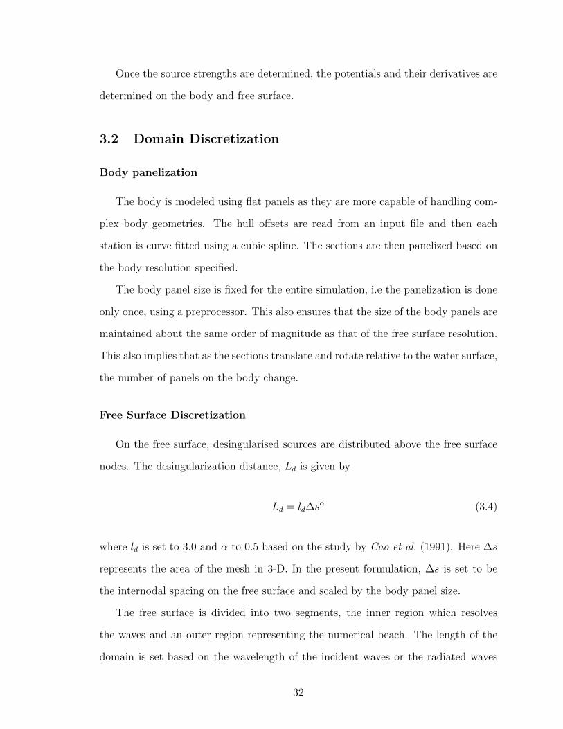
The inclusion of the sway and yaw viscous forces, dramatically change the results.
As can be seen from Figure 4.2, the additional viscous damping reduces the overshoot
of the slowly varying yaw response and quickly brings the vessel to a stable equilibrium
configuration. The steady state orientation has changed from being beam seas to
about 10o away from the expected beam sea configuration, bow into the waves. This
could be the effect of the change in the force balance between the 2nd order wave
drift forces, potential damping forces and viscous forces. This is reflected in the
trajectory of the ship, as seen in Figure 4.2(b), where the ship is drifting almost
along the direction of the wave fronts. The results could also be the effect of the
“double-counting” issue mentioned in Section 2.9, where part of the lift forces in the
hydrodynamic derivatives Yj, Nj(j = v, r) are being accounted for by the potential
forces.
The effects of the change in wave heading, slope and frequency is shown in Figures
4.3-4.5. All the simulations are done with viscous forces in sway and yaw. The final
steady state orientation of the vessel is between 10o and 15o away from the beam
43
sea configuration, depending on the incident wave parameters. It is to be mentioned
that in the case of head seas, with the vessel starting off in an unstable equilibrium
position, a small perturbation is given to the wave heading (made 179.95o) to kickstart
the free motions.
0 20 40 60 80 100 120 140 160 180−70
−60
−50
−40
−30
−20
−10
0
10
t/T(wave periods)
Mo
tio
ns(d
eg
)
Rotational motions
roll
pitch
yaw
Beam sea configuration
(a) Time history of yaw motions
−1 0 1 2−2
−1.5
−1
−0.5
0
0.5
1Trajectory
X/L
Y/L
(b) Track of ship
Figure 4.2: FREE MOTION DRIFT OF WIGLEY-I, λ/L = 1.0, H/λ = 1/50, WAVEDIRECTION= 45o, WITH SWAY-YAW VISCOUS FORCES
44

0 50 100 150 200 250 300 350 400−20
0
20
40
60
80
100
120
t/T(wave periods)
Mo
tio
ns(d
eg
)
Rotational motions
roll
pitch
yaw
Beam sea configuration
(a) Time history of yaw motions
−6 −4 −2 0 2 4 6−10
−8
−6
−4
−2
0
2Trajectory
X/L
Y/L
(b) Track of ship (dot represents aft of the ship)
Figure 4.3: FREE MOTION DRIFT OF WIGLEY-I, λ/L = 1.0, H/λ = 1/50, WAVEDIRECTION = HEAD SEAS, WITH SWAY-YAW VISCOUS FORCES
45

0 50 100 150 200 250 300 350−70
−60
−50
−40
−30
−20
−10
0
10
t/T(wave periods)
Motions(d
eg)
Rotational motions
roll
pitch
yawBeam sea configuration
(a) Time history of yaw motions
−1 0 1 2−2
−1.5
−1
−0.5
0
0.5
1Trajectory
X/L
Y/L
(b) Track of ship
Figure 4.4: FREE MOTION DRIFT OF WIGLEY-I, λ/L = 1.0, H/λ = 1/100,WAVE DIRECTION= 45o, WITH SWAY-YAW VISCOUS FORCES
46

0 50 100 150 200 250 300 350 400−70
−60
−50
−40
−30
−20
−10
0
10
t/T(wave periods)
Motions(d
eg)
Rotational motions
roll
pitch
yawBeam sea configuration
(a) Time history of yaw motions
−5 0 5 10−10
−5
0
5Trajectory
X/L
Y/L
(b) Track of ship (dot represents the aft of the ship)
Figure 4.5: FREE MOTION DRIFT OF WIGLEY-I, λ/L = 0.7, H/λ = 1/50, WAVEDIRECTION= 45o, WITH SWAY-YAW VISCOUS FORCES
47

S-175
The first of the free motion drift simulations of the containership S-175 is shown
in Figure 4.6. No viscous sway-yaw forces are modeled. As with all the simulations,
the ship is aligned at t = 0 with the positive xe axis. Waves are incident at 45o wrt
xe. The ship quickly changes its orientation from the initial configuration and after a
couple of overshoots past the beam sea configuration, enters into the slowly varying
response in a similar manner to the Wigley-I responses. Because of the fore and aft
asymmetry of the hull, the mean of the final stable state configuration is about −30o
wrt xe. This is about 15o away from the beam sea configuration, with the stern into
the waves. This is also evident from Figure 4.6(c), showing the track of the ship
with the orientations superimposed at different instances in time. Figures 4.6(b) and
4.6(d) show the details of the first order responses.
The effect of including sway and yaw viscous forces is seen in Figure 4.7. As with
the response of the Wigley-I, the overshoot is dampened down by 10o and the ship
settles quickly to a stable state configuration of about −62o wrt xe. It is interesting
to note that the new equilibrium is about 17o away from the beam sea configuration,
with bow into the waves. This also has an effect on the track of the ship as seen in
Figure 4.7(b), where the ship is drifting into the waves.
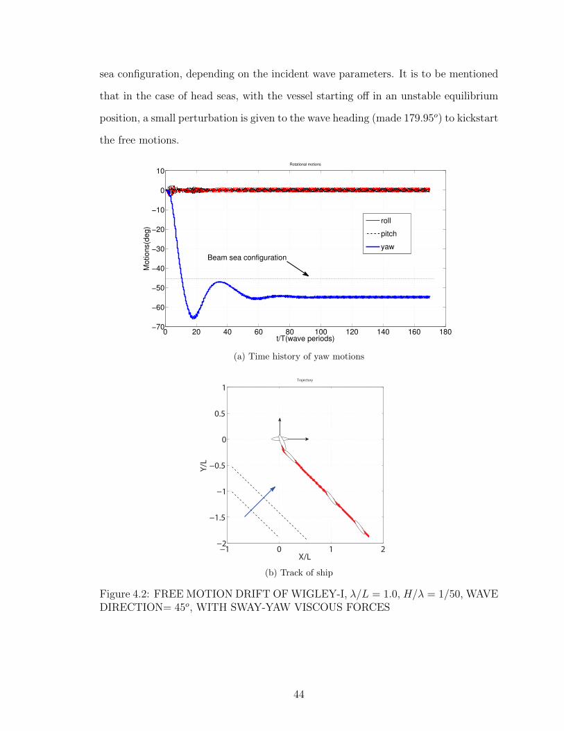
The effects of change in wave heading, slope and frequency is see seen in Figures
4.8 through 4.11. All the simulations are done with the sway and yaw viscous effects
on. The final steady state orientation of the vessel is between 15o and 17o away
from the beam sea configuration with bow into the waves, depending on the wave
characteristics.
48

050
100
150
200
250
300
−90
−80
−70
−60
−50
−40
−30
−20
−100
10
t/T
(wave p
eriods)
Motions(deg)
Ro
tatio
na
l m
otio
ns
roll
pitch
yaw
2
1
Beam
sea o
rienta
tion
(a)
Tim
eh
isto
ryof
yaw
moti
on
s
190
192
194
196
198
200
202
204
206
208
210
−2
−1.5−1
−0.50
0.51
1.52
t/T
(wave p
eriods)
Motions(deg)
Rota
tional m
otions
roll
pitch
(b)
Det
ail
sof
roll
an
dp
itch
moti
on
sfr
om
inse
t1
−5
05
10
15
−10
−505
10
Trajectory
X/L
Y/L
(c)
Tra
ckof
ship
18
51
90
19
52
00
20
52
10
21
5−
36
−3
4
−3
2
−3
0
−2
8
−2
6
−2
4
t/T
(wa
ve
pe
rio
ds)
Motions(deg)
Ro
tatio
na
l m
otio
ns
(d)
Det
ail
sof
yaw
moti
on
sfr
om
inse
t2
Fig
ure
4.6:
FR
EE
MO
TIO
ND
RIF
TO
FS-1
75,λ/L
=1.
0,H/λ
=1/
50,W
AV
ED
IRE
CT
ION
=45
o,N
OSW
AY
-YA
WV
ISC
OU
SF
OR
CE
S
49

0 50 100 150 200 250 300−70
−60
−50
−40
−30
−20
−10
0
10
t/T(wave periods)
Motions(d
eg)
Rotational motions
roll
pitch
yaw
1
2
Beam sea orientation
(a) Time history of yaw motions
−5 0 5 10 15 20−20
−15
−10
−5
0
5Trajectory
X/L
Y/L
(b) Track of ship
Figure 4.7: FREE MOTION DRIFT OF S-175, λ/L = 1.0, H/λ = 1/50, WAVEDIRECTION= 45o, WITH SWAY-YAW VISCOUS FORCES
50

0 50 100 150 200 250 300 350 400−20
0
20
40
60
80
100
t/T(wave periods)
Motions(d
eg)
Rotational motions
roll
pitch
yaw
Beam sea orientation
(a) Time history of yaw motions
−8 −6 −4 −2 0 2 4−8
−6
−4
−2
0
2
4Trajectory
X/L
Y/L
(b) Track of ship
Figure 4.8: FREE MOTION DRIFT OF S-175, λ/L = 1.0, H/λ = 1/50, WAVEDIRECTION= 180o, WITH SWAY-YAW VISCOUS FORCES
51

0 50 100 150 200 250 300 350 400−80
−70
−60
−50
−40
−30
−20
−10
0
10
t/T(wave periods)
Mo
tio
ns(d
eg
)
Rotational motions
roll
pitch
yawBeam sea orientation
2
1
(a) Time history of yaw motions
−2 0 2 4 6 8−8
−6
−4
−2
0
2Trajectory
X/L
Y/L
(b) Track of ship
Figure 4.9: FREE MOTION DRIFT OF S-175, λ/L = 1.0, H/λ = 1/100, WAVEDIRECTION= 45o, WITH SWAY-YAW VISCOUS FORCES
52
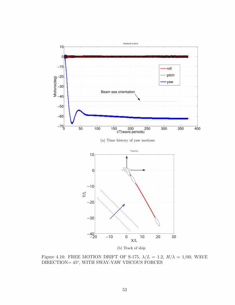
0 50 100 150 200 250 300 350 400−70
−60
−50
−40
−30
−20
−10
0
10
t/T(wave periods)
Mo
tio
ns(d
eg
)
Rotational motions
roll
pitch
yaw
Beam sea orientation
(a) Time history of yaw motions
−20 −10 0 10 20 30−40
−30
−20
−10
0
10Trajectory
X/L
Y/L
(b) Track of ship
Figure 4.10: FREE MOTION DRIFT OF S-175, λ/L = 1.2, H/λ = 1/60, WAVEDIRECTION= 45o, WITH SWAY-YAW VISCOUS FORCES
53

0 50 100 150 200 250 300 350−70
−60
−50
−40
−30
−20
−10
0
10
t/T(wave periods)
Mo
tio
ns(d
eg
)
Rotational motions
roll
pitch
yawBeam sea orientation
(a) Time history of yaw motions
−10 −5 0 5−5
0
5
10Trajectory
X/L
Y/L
(b) Track of ship
Figure 4.11: FREE MOTION DRIFT OF S-175, λ/L = 0.7, H/λ = 1/50, WAVEDIRECTION= 45o, WITH SWAY-YAW VISCOUS FORCES
54

CHAPTER V
Maneuvering Results
The turning circle maneuvers of the containership S-175 are simulated in calm
water and regular waves, and compared with experiments conducted by Yasukawa
and Nakayama (2009). The propeller thrust, the hull resistance, rudder forces, and
viscous linear and nonlinear forces in sway and yaw, are modeled according to Son
and Nomoto (1981). The basic details are given in Section 2.9. The main particulars
of the hull, rudder and propeller are given in Table 5.1.
As mentioned in Section 2.9, the models in Son and Nomoto (1981) for the S-
175, make use of semi-empirical parameters and coefficients to account for hull wake,
rectification of the flow from the propeller to the rudder, and to model the rudder
lift forces. In the present computations, no attempt has been made to tune these
parameters to obtain a better fit with experiments.
5.1 Calm Water Turning Circle Test
At t = 0, the propeller is turned on and the ship is allowed to come up to the
approach speed set at 6.212 m/s (Fn = 0.15). The propeller rps (revolutions/sec) to
achieve this speed is calculated from the thrust-resistance balance and set at 0.9893
rps. In order to keep the ship on course, an automatic 4-DOF based nonlinear con-
troller developed by Li et al. (2010) is used. At t = 1200 s, the rudder is put over at
55

LBP [m] 175.0B [m] 25.4T [m] 9.5S [m2] 5540CW 0.7080CB 0.5714
Rudder area [m2] 33.04Aspect ratio 1.8219
Propeller diameter [m] 6.533
Table 5.1: DETAILS OF CONTAINERSHIP S-175
maximum deflection of δ = −35o to execute a tight starboard turn. The maximum
rudder deflection rate is set to δ = 5o/s. The track of the ship is shown in Figure 5.1.
The results from the experimental data in Yasukawa and Nakayama (2009) is also
shown for comparison. As can be seen from the plots, the agreement is quite good.
The advance, transfer and steady turning diameter are in close agreement to the ex-
perimental values. The tactical diameter is off by about 0.8 shiplength. One possible
explanation for this could be due to the additional lift forces and moments that are
generated from the potential theory and the issue of “double-counting” mentioned in
Section 2.9. Figures 5.1 (b) and (c) show the time-history of the translational and
rotational velocities of the hydrodynamic frame as it is maneuvering.
5.2 Turning Circle Test in Regular Waves
The turning circle tests are performed for the containership S-175 in the presence
of regular waves. Wave headings of θ = 90o (Beam seas) and θ = 180o (Head seas)
are considered and λ/L is set to 0.7, 1.0, and 1.2. In order to compare with the
available experimental results from Yasukawa and Nakayama (2009), the wave height
is set equal to 3.5 m. This would correspond to H/L = 1/50, which implies the wave
steepness changes with wavelength of the incident waves. As with the case of the
calm water maneuvering test, the ship is brought up to an approach speed of 6.212
56
−4 −2 0 2 4−6
−5
−4
−3
−2
−1
0
1
2Trajectory
X/L
Y/L
Numerical modelExperiments
(a) Trajectory
0 500 1000 1500 2000 2500 3000−1
0
1
2
3
4
5
6
7
time(s)
velo
city (
m/s
)
Plots of U and V
UV
(b) Velocities U and V of hydrodynamic frame
0 500 1000 1500 2000 2500 3000−12
−10
−8
−6
−4
−2
0
2x 10
−3 yaw rate:
time(s)
yaw
rate
(ra
ds/s
)
(c) Yawrate ψ of hydrodynamic frame
Figure 5.1: CALM WATER TURNING CIRCLE OF S-175, δ = −35o
57

m/s (Fn = 0.15) and once steady state is reached (t = 1200 s), the rudder is put
hard over and simultaneously, the waves are turned on. A brief linear ramp of two
periods is used to bring the waves to full wave height.
Figures 5.2 and 5.3 show the results of the starboard (δ = −35o) turning circle
test for λ/L = 1.0 in beam seas. The arrow in Figure 5.2(a) indicates the direction of
the waves and the shows the track of the ship. As can be seen, the model reasonably
captures the general characteristics of the turn. The ship enters into a series of
steady turning circle loops, along with a net drift due to the wave drift forces. It
is interesting to note that there are drift components both along and perpendicular
to the direction of the wave fronts. Although the steady turning diameter, advance,
transfer and tactical diameter are being over-predicted, the overall course and drift of
the ship is in the right direction. Figures 5.2(b) and 5.2(c) show interesting results for
the translational and rotational velocities of the hydrodynamic frame, respectively.
The model captures the increase and decrease of the velocities at different phases of
the turn. As can be seen, the oscillatory component of the velocities is superimposed
on the time-varying mean component. Figure 5.3 shows the details of roll, pitch
and heave motions during the turning maneuver, of inset 1 in Figure 5.3(a). The
interesting feature here is that as the ship traverses from a following sea configuration,
through beam sea and into head sea, there is a shift in the frequency of encounter.
This is evident from plots 5.3(b) and 5.3(c).
Figures 5.4-5.12 show the turning circle results for λ/L = 1.0, λ/L = 1.2, and
λ/L = 0.7 for beam and head seas. For λ/L = 1.0 and λ/L = 1.2, the ship is able to
enter into a series of loop to loop turns and drift in the right direction. The advance,
transfer and turning diameter are being over-predicted by the present method. In
general, it is observed that the rudder is encountering large opposing forces that are
delaying the turning rate. This looks more apparent when the ship is in a following
sea configuration. It also indicates that the forward speed is much higher than what
58

it should be, which results in a much larger turning diameter. The other issue is
that of “double-counting”, where the rudder is facing the opposing forces of viscous
maneuvering forces Yj, Nj (j = v, r) as well as the forces being generated from the
potential theory. The other source of over-prediction could be with the prediction of
the 2nd order wave drift forces and moments. It is known that as the wavelengths
get shorter, the drift forces get larger. This is apparent from Figures 5.11 and 5.12,
which represent the starboard and portside turning maneuver for λ/L = 0.7 in beam
seas, respectively. The ship is being drifted by a large amount when it is in following
sea condition. From Figure 5.11, it is seen that the ship in fact begins the turn
pretty much in agreement with the experiments, before it turns around and enters the
following sea configuration and begins being drifted a long way before the rudder can
again turn the ship around. The turning tests for λ/L = 0.7 are done in relatively
steep waves of H/λ = 1/35. In order to ensure that the incorrect drift is not a
frequency related issue, the wave height was reduced, such that H/λ = 1/50, and the
turn simulated. The result is shown in Figure 5.13, where the ship is drifting in the
right direction. The other issue could also be that since the rudder model parameters
are not tuned in any way, the lift forces produced by the rudder are not strong enough
to tighten the turns.
The effect of changing the initial phase angle of the incident waves is seen in Figure
5.14. An initial phase angle of 0o corresponds to a wave crest at midships at t = 0,
and initial phase angle of 90o corresponds to a zero crossing at t = 0. The shift in
phase does not have an effect on the 2nd order wave drift forces, but as can be seen
from the details in Figure 5.14(b), there is a phase shift in the first order response as
expected.
59

−4
−2
02
46
−6
−4
−2024
Tra
jecto
ry
X/L
Y/L
Nu
me
rica
l m
od
el
Exp
erim
en
ts
1
(a)
Tra
ject
ory
10
00
15
00
20
00
25
00
30
00
35
00
−101234567
tim
e(s
)
velocity (m/s)
Plo
ts o
f U
an
d V
U V
(b)
Vel
oci
ties
Uan
dV
ofhyd
rod
yn
am
icfr
am
e
1000
1500
2000
2500
3000
3500
−0.0
25
−0.0
2
−0.0
15
−0.0
1
−0.0
050
0.0
05
ya
w r
ate
:
tim
e(s
)
yaw rate (rads/s)
(c)
Yaw
rateψ
of
hyd
rod
yn
am
icfr
am
e
Fig
ure
5.2:
TU
RN
ING
CIR
CL
EO
FS-1
75IN
WA
VE
S,δ
=−
35o,λ/L
=1.
0,H
EA
DIN
G=
BE
AM
SE
AS,H/λ
=1/
50
60

−4
−2
02
46
−6
−4
−2024
Tra
jecto
ry
X/L
Y/L
Nu
me
rica
l m
od
el
Exp
erim
en
ts
1
(a)
Tra
ject
ory
17
01
75
18
01
85
19
01
95
20
02
05
21
02
15
22
02
25
−4
−3
−2
−1012345
t/T
(w
ave
pe
rio
ds)
Motions(deg)
Ro
tatio
na
l m
otio
ns
roll
pitch (b
)D
etai
lsof
roll
and
pit
chm
oti
on
s
170
175
180
185
190
195
200
205
210
215
220
225
−1.5−1
−0.50
0.51
1.5
He
ave
mo
tio
ns
t/T
(wave p
eriods)
η3/A
Heave
(c)
Det
ail
sof
hea
ve
moti
on
s
Fig
ure
5.3:
DE
TA
ILS
OF
RO
LL
,P
ITC
HA
ND
HE
AV
ED
UR
ING
TU
RN
ING
MA
NE
UV
ER
,δ
=−
35o,λ/L
=1.
0,H
EA
DIN
G=
BE
AM
SE
AS,H/λ
=1/
50
61

−4 −2 0 2 4 6−2
0
2
4
6
8Trajectory
X/L
Y/L
Numerical modelExperiments
Figure 5.4: TURNING CIRCLE OF S-175 IN WAVES, δ = 35o, λ/L = 1.0, HEAD-ING = BEAM SEAS, H/λ = 1/50
62

−4 −2 0 2 4 6−2
0
2
4
6
8Trajectory
X/L
Y/L
Numerical modelExperiments
Figure 5.5: TURNING CIRCLE OF S-175 IN WAVES, δ = 35o, λ/L = 1.0, HEAD-ING = HEAD SEAS, H/λ = 1/50
63

−4 −2 0 2 4 6−6
−4
−2
0
2
4Trajectory
X/L
Y/L
Numerical modelExperiments
Figure 5.6: TURNING CIRCLE OF S-175 IN WAVES, δ = −35o, λ/L = 1.0, HEAD-ING = HEAD SEAS, H/λ = 1/50
64

−4 −2 0 2 4 6−6
−4
−2
0
2
4Trajectory
X/L
Y/L
Numerical modelExperiments
Figure 5.7: TURNING CIRCLE OF S-175 IN WAVES, δ = −35o, λ/L = 1.2, HEAD-ING = HEAD SEAS, H/λ = 1/60
65

−4 −2 0 2 4 6−6
−4
−2
0
2
4Trajectory
X/L
Y/L
Numerical modelExperiments
Figure 5.8: TURNING CIRCLE OF S-175 IN WAVES, δ = −35o, λ/L = 1.2, HEAD-ING = BEAM SEAS, H/λ = 1/60
66

−4 −2 0 2 4 6−2
0
2
4
6
8Trajectory
X/L
Y/L
Numerical modelExperiments
Figure 5.9: TURNING CIRCLE OF S-175 IN WAVES, δ = 35o, λ/L = 1.2, HEAD-ING = HEAD SEAS, H/λ = 1/60
67

−4 −2 0 2 4 6−2
0
2
4
6
8Trajectory
X/L
Y/L
Numerical modelExperiments
Figure 5.10: TURNING CIRCLE OF S-175 IN WAVES, δ = 35o, λ/L = 1.2, HEAD-ING = BEAM SEAS, H/λ = 1/60
68
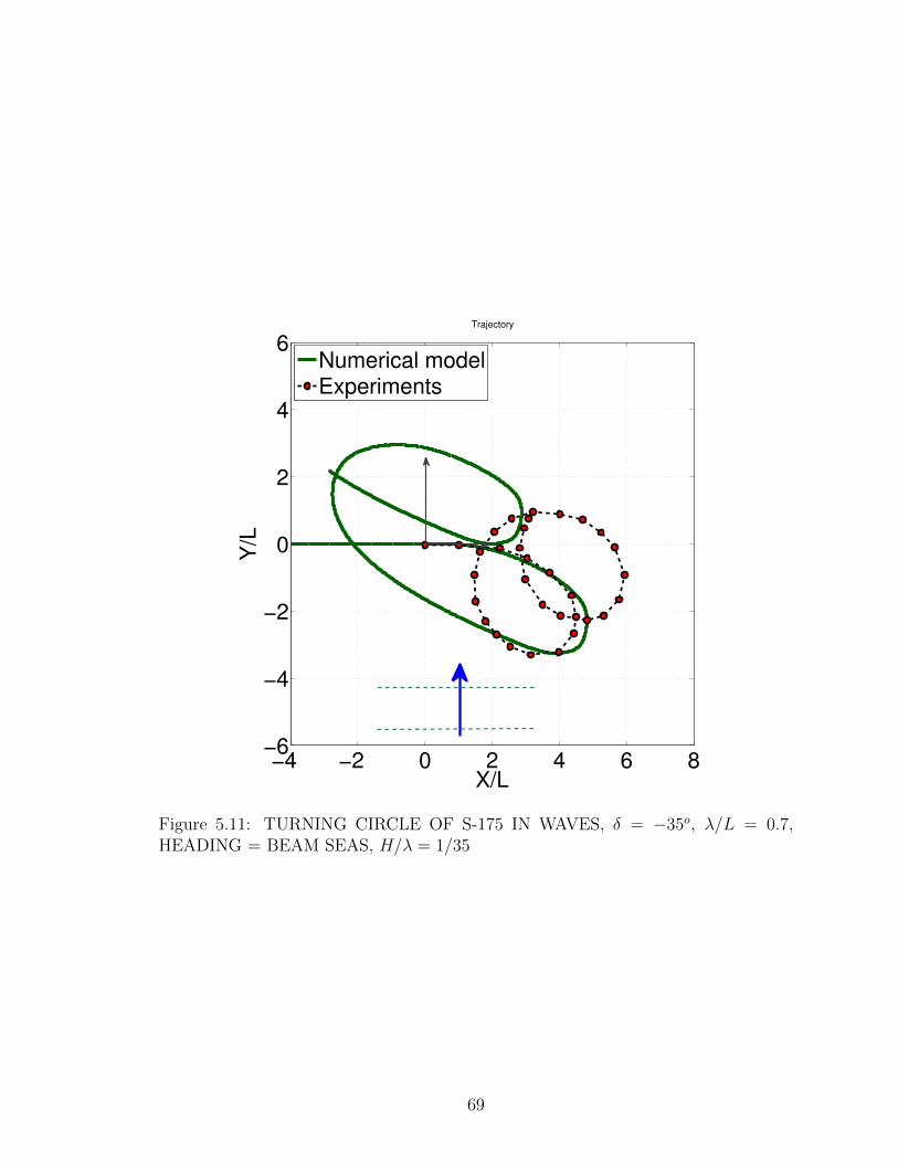
−4 −2 0 2 4 6 8−6
−4
−2
0
2
4
6Trajectory
X/L
Y/L
Numerical modelExperiments
Figure 5.11: TURNING CIRCLE OF S-175 IN WAVES, δ = −35o, λ/L = 0.7,HEADING = BEAM SEAS, H/λ = 1/35
69

−4 −2 0 2 4 6 8−2
0
2
4
6
8
10Trajectory
X/L
Y/L
Numerical modelExperiments
Figure 5.12: TURNING CIRCLE OF S-175 IN WAVES, δ = 35o, λ/L = 0.7, HEAD-ING = BEAM SEAS, H/λ = 1/35
70

−4 −2 0 2 4 6−2
0
2
4
6
8Trajectory
X/L
Y/L
Figure 5.13: TURNING CIRCLE OF S-175 IN WAVES, δ = 35o, λ/L = 0.7, HEAD-ING = BEAM SEAS, H/λ = 1/50
71

−4 −2 0 2 4 6
0
2
4
6
8
X/L
Y/L
phase angle = 0 degsphase angle = 90 degs
(a) Trajectory
1.1 1.2 1.31.6
1.65
1.7
1.75
1.8
1.85
1.9
X/L
Y/L
phase angle = 0 degsphase angle = 90 degs
(b) Details of inset
Figure 5.14: EFFECT OF INITIAL PHASE ANGLE OF INCIDENT WAVES, δ =35o, λ/L = 1.0, HEADING = BEAM SEAS, H/λ = 1/50
72

CHAPTER VI
Surge Damping Model
Although potential theory has proven to be a robust and powerful seakeeping
prediction tool, it cannot predict viscous forces. For the horizontal plane motions,
this is crucial due to lack of restoring forces. The viscous force models have been
elaborated in this research work in Chapters II, IV and V. In this chapter, the surge
force prediction capability of the strip theory approach is examined.
The present formulation is used to predict the surge force on the Wigley-I hull
that is set into forced surge oscillations, towed at a constant forward speed. A simple
empirical damping model is proposed and the force is added to the results from
potential theory. The results from the simulations are compared with the results
predicted by an Unsteady Reynolds-Averaged Navier-Stokes (URANS) equation CFD
solver-openFOAM.
6.1 Empirical Scheme
A simple “quasi-steady” formulation in which the surge force is proportional to
the instantaneous forward speed, is proposed to model the surge damping, Fsurge
given by:
Fsurge = −1
2cDρSu(t)|u(t)| (6.1)
73

LBP [m] 4.0B [m] 0.4T [m] 0.25S [m2] 2.3796CW 0.6886CB 0.5571
Table 6.1: DETAILS OF WIGLEY-I HULL
where ρ and S are the density of fluid, and the wetted surface area, respectively. cD
is the drag coefficient based on the calm water resistance of the ship. The forward
speed u(t) is the instantaneous surge velocity. Therefore, this model predicts both
the calm water resistance as well as the surge oscillatory damping.
6.2 URANS Formulation
The viscous flow solver is based on the open source CFD library OpenFOAM. It
basically solves the URANS equations and uses a VOF method for interface capturing.
The package is heavily customizable with a wide variety of options to specify the
type of computational elements, solution gradients, discretization schemes for the
convection and advection terms, interface-capturing schemes, type of solver for the
transport equations and governing equations etc. It can also be run in parallel to
speed up the computations.
6.3 Results and Discussion
The Wigley-I hull is used for the computations. The details are given in Table 6.1.
The test matrix for the study is given in Table 6.2. The nondimensional frequency
ω∗ = ω√L/g used in the study, spans the normal range of frequencies used in sea-
keeping analysis. The amplitude of motion, A is set such that (2A)/λ, the wave slope
of the radiated waves is 1/60. Interestingly, this also implies that the amplitude of
the acceleration of the body, Aω2 is constant across the frequency range. The forward
74

Run id 1 2 3 4 5λ/L 0.5 1.0 1.5 2.0 2.5
A [m] 0.0167 0.0334 0.0500 0.0667 0.0834T [s] 1.1323 1.6013 1.9612 2.2646 2.5318
ω (rads/s) 5.5490 3.9238 3.2037 2.7745 2.4817ω∗ 3.54 2.51 2.05 1.77 1.58AωU
0.049 0.071 0.085 0.099 0.110
Table 6.2: TEST MATRIX FOR FORCED SURGE PROBLEM
speed, U of the hull is set to 1.88 m/s, corresponding to a Froude number of 0.3.
Potential Flow Details
The present method uses 40 panels on the body, per station. The number of
nodes/wavelength on the free surface is set to 30 and the computational domain
length is set to 4 wavelengths on each side, including 2 wavelengths for the numerical
beach. A time step size of T/200 is used for the numerical integration on the free
surface.
OpenFOAM CFD Solver
The computational domain shown in Figure 6.1 extends from one ship-length
upstream to 3L downstream. The lateral domain extends to one ship-length form the
centreline and the bottom is set at 0.75L below the calm water level. The domain for
the air column extends to 0.1875L. The number of cells used in the computations is
163, 580. This is considered a coarse grid.
Calm Water Resistance
The calm water resistance of the Wigley hull at Fn = 0.3 is computed by using
the OpenFOAM solver. Figure 6.2 shows the wave patterns generated by the ship.
The computations were run out to 100 s to allow for the transients to decay. The
dynamic pressure on the hull surface with the high pressure bow region, is shown in
75

Figure 6.3. The calm water resistance is computed by integrating the pressure and
shear stress on the hull surface. The calm water resistance time history is shown in
Figure 6.4 with both the pressure and viscous components. The value of Fcalm, the
calm water resistance, is calculated to be 18.9860 N by averaging over the last few
cycles. The value from the experiments is about 20 N, which is a difference of 5%.
This is used to compute the value of cD to be used in the empirical model, which
turns out to be 4.4047× 10⁻³.
Forced surge motions
The forced surge motions are performed by using the test matrix in Table 6.2
as input to both the body-exact potential flow solver, and the OpenFOAM URANS
solver. The simulations are run for 50 periods. The surge force from the damping
model is added to the potential theory results.
Figures 6.5 - 6.9, show the surge force time history for the 5 test cases from
λ/L = 0.5 to λ/L = 2.5. Comparisons are made between the forces predicted with
and without the damping model, to the CFD results. It is observed that the potential
theory formulation, underpredicts the force compared to CFD, while the surge force
model overpredicts it. As expected, the potential theory gives better results at higher
frequencies, and gets worse as frequency drops, eventually predicting zero damping at
ω = 0. On the other hand, potential theory predicts the forces within a good level of
accuracy for the higher frequencies, in particular, for λ/L ≤ 1.0. The results suggest
that although the damping model does help in correcting the values from potential
theory, it is overpredicting the values, and thus may need to be carefully augmented
based on the frequency. One solution would be in the manner that Bailey et al. (1997)
used a linear ramp to correct the potential theory sway and yaw forces by adding the
maneuvering derivatives as viscous effect corrections. Figures 6.11 and 6.12 are the
frequency domain results obtained by running the time domain results through a
76

FFT routine. It gives a better perspective of the model used and can be used to
improve the empirical method to correct the potential flow results. The combined
wave systems of the steady forward speed problem and forced surge oscillations are
shown in Figure 6.10.
77

Figure 6.1: OpenFOAM COMPUTATIONAL DOMAIN
Figure 6.2: CALM WATER WAVE PATTERN, Fn = 0.30 (OpenFOAM)
78

Figure 6.3: DYNAMIC PRESSURE ON HULL SURFACE, Fn = 0.30 (OpenFOAM)
0 20 40 60 80 100−20
−10
0
10
20
30
40
time(s)
Resis
tance(N
)
Resistance on Wigley hull Fn=0.3
pressureviscousTotal
Figure 6.4: CALM WATER RESISTANCE, Fn = 0.30 (OpenFOAM)
79

30 32 34 36 38 40−1.5
−1
−0.5
0
t/T (wave periods)
Fsu
rge/R
ca
lm
Surge force on Wigley hull Fn=0.3
CFDTotal
Potential + Empirical modelPotential only
Figure 6.5: SURGE FORCE λ/L = 0.5
30 32 34 36 38 40−1.5
−1
−0.5
0
t/T
Fsu
rge/R
ca
lm
Surge force on Wigley hull Fn=0.3
CFDTotal
Potential + Empirical modelPotential only
Figure 6.6: SURGE FORCE λ/L = 1.0
80
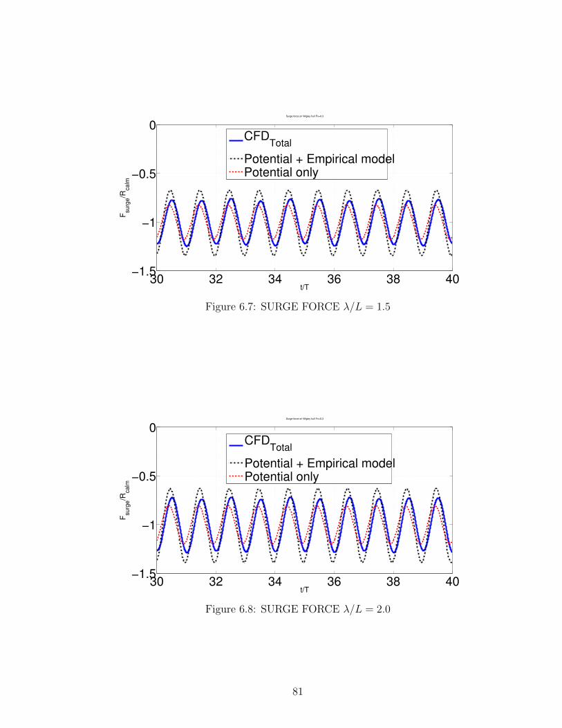
30 32 34 36 38 40−1.5
−1
−0.5
0
t/T
Fsu
rge/R
ca
lm
Surge force on Wigley hull Fn=0.3
CFDTotal
Potential + Empirical modelPotential only
Figure 6.7: SURGE FORCE λ/L = 1.5
30 32 34 36 38 40−1.5
−1
−0.5
0
t/T
Fsu
rge/R
ca
lm
Surge force on Wigley hull Fn=0.3
CFDTotal
Potential + Empirical modelPotential only
Figure 6.8: SURGE FORCE λ/L = 2.0
81

30 32 34 36 38 40−1.5
−1
−0.5
0
t/T
Fsu
rge/R
ca
lm
Surge force on Wigley hull Fn=0.3
CFDTotal
Potential + Empirical modelPotential only
Figure 6.9: SURGE FORCE λ/L = 2.5
Figure 6.10: FREE SURFACE, FORCED SURGE λ/L = 2.5
82

0 0.5 1 1.5 2 2.5 35
10
15
20
25
30
35
40
45Comparison of FFT results of force time history: Amplitude
λ/L
Fsu
rge/R
ca
lm*1
00
CFD
Potential + Empirical model
Potential only
Figure 6.11: COMPARISON OF FORCE AMPLITUDES FROM FFT ANALYSIS
0 0.5 1 1.5 2 2.5−100
0
100
200
300
400Comparison of FFT results of force time history: Phase
λ/L
Ph
ase
(d
eg
s)
CFD
Potential + Empirical model
Potential only
Figure 6.12: COMPARISON OF FORCE PHASE FROM FFT ANALYSIS
83

CHAPTER VII
Conclusions and Recommendations
A body-exact strip theory has been developed to simulate maneuvering of a ship
in a seaway. Free motion drift simulations have been performed on the Wigley-I and
containership S-175. The long time simulations establish the ability of the translating
and rotating hydrodynamic axis system in predicting the drift and steady state stable
equilibrium configuration of the ship wrt the waves. Both first order responses at
the wave frequency, and higher order slowly varying drift motions are captured. The
results also establish the stability of the numerical scheme and the numerical damping
beach by the ability to simulate hundreds of wave periods. The methodology is robust
enough to handle realistic hull forms like the S-175 with a bulbous bow and transom
stern.
Propeller thrust force, calm water resistance, viscous forces and rudder lift forces
are modeled based on semi-empirical methods, to predict the turning circle maneuver
of the containership S-175 in calm waters and in the regular waves. The qualitative
aspects of the maneuver are captured by the numerical model, in particular for longer
waves.
In order to make quantitative comparisons, there are issues that need to be ad-
dressed. In the present methodology, the potential theory predicts lift forces and mo-
ments. The steady potential corresponding to the time-varying mean component of
84

the body velocity is also solved for in the present formulation. In a three-dimensional
linear potential method, there would be no lift forces generated on a body. The forces
predicted by the present method could be an artifact of strip theory, so one solution
would be to avoid solving the steady velocity potential and only solve for the oscil-
latory component. Another approach would be to reduce the viscous forces to avoid
“double-counting” the hull lift forces.
Improved models for predicting the rudder forces and propeller rudder interactions
are needed. The models that are used in the present computations are directly from
the ones used in Son and Nomoto (1981). No attempt has been made to tune these
coefficients to improve the prediction. Since the model is known to be sensitive to
these parameters, it is crucial to correctly account for these factors. It is also to be
noted that, the present simulations do not consider the side force from the propeller,
which can be quite a significant percentage of the forward thrust.
Radial basis functions are used to compute the x-derivative. Although their reli-
ability has shown to be sufficient, there is scope for improvement by use of improved
basis functions. They are also one of the most time-consuming routines in the com-
puter code, so improvements in the efficiency of these routines could also translate to
much faster computational times.
A simple empirical surge damping model has been proposed and used to correct
the surge force predictions made by the potential theory. Comparisons are made
with results obtained from CFD. Although, the model does correct the potential flow
results, they are being overpredicted. The analysis does provide a basis to improve
the damping model by considering a correction factor, such as the linear ramp that
is used in Bailey et al. (1997).
85

APPENDICES
86

APPENDIX A
Convergence Results
Any numerical scheme must be studied for convergence. This gives a handle on
the maximum value of the resolution, that gives an acceptable solution. The studies
are done for two scenarios. The first set of convergence studies is done for the forced
heave problem of the Wigley-I hull form. The convergence study with respect to
time-step size is also done for the free motion drift problem of the Wigley-I. This is
important because, since the simulations are being done for long times, quantities
like body accelerations and velocities are integrated in time, causing accumulation of
the integration errors at each time-step.
A.1 Forced Heave Problem
The Wigley-I hull is set into forced heave motions, and the heave force is used to
study convergence characteristics. The details of the hull are given in Table 4.1 in
Chapter IV. The frequency of oscillations is chosen such that, the wavelength, λ to
shiplength, L ratio is λ/L = 1.25. The amplitude of motions, A is set equal to about
15% of the draft, T .
Three parameters are studied in the problem, namely, the time-step size, number
of body panels, and the free surface domain size. It is to be noted that, the free
87

surface resolution is not entirely independent of the body resolution. In order to
maintain good condition number of the influence matrix, the free surface resolution
has to be of the same order of magnitude as the body resolution. It is observed that
for convergence of the solution, there is a minimum free surface resolution required
for a given body resolution. Therefore, in these tests, the free surface resolution is
changed proportionately to the body resolution. The time-step size is based on the
period of the radiated waves. The free surface domain is based on the size of the inner
region. The outer region, consisting of the damping beach, is set to two wavelengths
and fixed.
The convergence is studied, by changing one parameter at a time, keeping the
others fixed at a high resolution value deemed sufficient for converged results. The
results are shown in figures A.1 - A.3. As can be see, the convergence w.r.t the time-
step size is fast. Based on the results, 50 panels on the body, a free surface resolution
of λ/30 and free surface domain length of 2 wavelengths is considered as a set of
parameters to have a good balance between computational speed and accuracy.
A.2 Free Motion Drift
As an additional check, the convergence is also studied for the free motion drift
problem of the Wigley-I in the presence of external waves. The convergence is studied
with respect to the time-step size, to ensure that the solution is not affected by
accumulation of integration errors. The results are shown for the track and yaw
motion time history in figures A.4 and A.5, respectively.
88

0 1 2 3 4 5 6 7 8 9 10−150
−100
−50
0
50
100
150
200
time(s)
Fo
rce
(N)
25 panels 50 panels 100 panels 150 panels
(a) Time history of heave force
5.7 5.72 5.74 5.76 5.78 5.8 5.82 5.84
129.5
130
130.5
131
131.5
132
132.5
133
133.5
134
134.5
time(s)
Fo
rce
(N)
25 panels 50 panels 100 panels 150 panels
(b) Details
Figure A.1: CONVERGENCE STUDIES FOR NUMBER OF BODY PANELS,FREE SURFACE RESOLUTION FOR 25 BODY PANELS = λ/30, 50 BODY PAN-ELS = λ/60, 100 BODY PANELS = λ/60, 150 BODY PANELS = λ/90. TIME-STEPSIZE = T/200. FREE SURFACE INNER DOMAIN = 2 WAVELENGTHS.
89
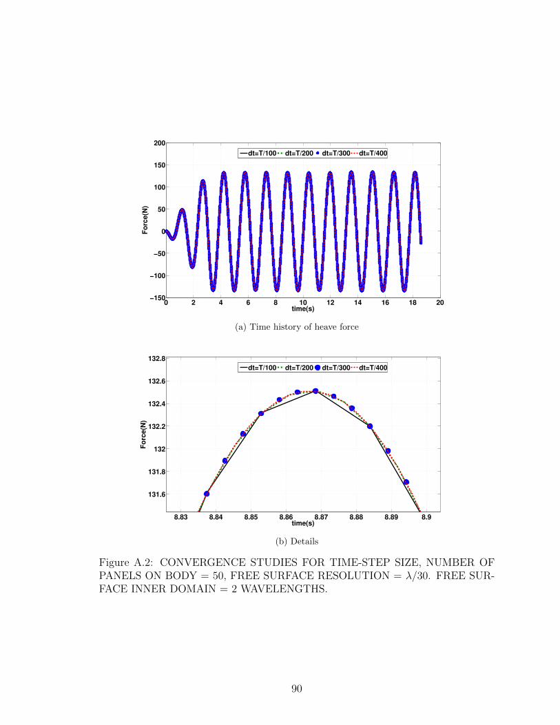
0 2 4 6 8 10 12 14 16 18 20−150
−100
−50
0
50
100
150
200
time(s)
Fo
rce
(N)
dt=T/100 dt=T/200 dt=T/300 dt=T/400
(a) Time history of heave force
8.83 8.84 8.85 8.86 8.87 8.88 8.89 8.9
131.6
131.8
132
132.2
132.4
132.6
132.8
time(s)
Fo
rce
(N)
dt=T/100 dt=T/200 dt=T/300 dt=T/400
(b) Details
Figure A.2: CONVERGENCE STUDIES FOR TIME-STEP SIZE, NUMBER OFPANELS ON BODY = 50, FREE SURFACE RESOLUTION = λ/30. FREE SUR-FACE INNER DOMAIN = 2 WAVELENGTHS.
90
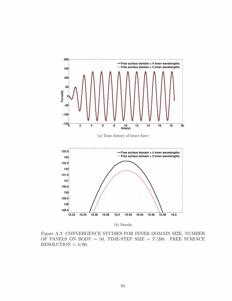
0 2 4 6 8 10 12 14 16 18 20−150
−100
−50
0
50
100
150
200
time(s)
Fo
rce
(N)
Free surface domain = 4 inner wavelengths
Free surface domain = 2 inner wavelengths
(a) Time history of heave force
10.32 10.34 10.36 10.38 10.4 10.42 10.44 10.46 10.48 10.5
128.5
129
129.5
130
130.5
131
131.5
132
132.5
133
133.5
Free surface domain = 4 inner wavelengths
Free surface domain = 2 inner wavelengths
(b) Details
Figure A.3: CONVERGENCE STUDIES FOR INNER DOMAIN SIZE, NUMBEROF PANELS ON BODY = 50, TIME-STEP SIZE = T/200. FREE SURFACERESOLUTION = λ/60.
91

(a) Track of ship
(b) Details of track of ship
Figure A.4: TRACK OF SHIP-CONVERGENCE STUDIES FOR TIME-STEPSIZE, FREE MOTION DRIFT OF WIGLEY-I, NUMBER OF PANELS ON BODY= 50, REFERENCE TIME-STEP SIZE δt= T/200. FREE SURFACE RESOLU-TION = λ/30, FREE SURFACE INNER DOMAIN = 2 WAVELENGTHS.
92

(a) Yaw motion time history
(b) Details of yaw motions
Figure A.5: YAW MOTIONS OF SHIP - CONVERGENCE STUDIES FOR TIME-STEP SIZE, FREE MOTION DRIFT OF WIGLEY-I, NUMBER OF PANELS ONBODY = 50, REFERENCE TIME-STEP SIZE δt= T/200. FREE SURFACE RES-OLUTION = λ/30, FREE SURFACE INNER DOMAIN = 2 WAVELENGTHS.
93

APPENDIX B
Validation of Computer Code
Computer codes are prone to bugs and programming errors. It is therefore, impor-
tant to validate the code by performing suitable tests. Since the present methodology
is designed to handle a variety of hull forms, where the length scales of the problem
could range from model scale to full scale, the code is tested for invariance with re-
spect to scale. Also, since the physics of the problem is independent of the coordinate
reference frame used, the code is tested for invariance with respect to the coordinate
frame.
B.1 Scale Factor Test
The Wigley-I hull is set into forced heave oscillations, and the heave force is used
to verify the invariance of the problem with respect to the scale factor. Two sets of
computations are performed, one at model scale and the other at a scale factor of 60.
The forces are compared by nondimensionalising the heave force by 12ρL2(Aω)2. The
details of the parameters used for the test are given in Table B.1.
The results for the scale factor test is given in Figure B.1. The details in Figure
B.1(b) highlight the differences in solution, when the input is scaled by a factor of
94

Scale factor 1 60LBP[m] 3.0 180.0
B[m] 0.3 18.0T[m] 0.1875 11.25S[m2] 1.3385 4818.6CW 0.6886 0.6886CB 0.5571 0.5571
ω[rads/s] 4.0525 0.5232A[m] 0.0250 1.5
Table B.1: WIGLEY-I PARTICULARS FOR SCALE FACTOR TEST
60. The difference is in the 3rd decimal place, a variation of 0.16% compared to scale
= 1. The difference could be attributed to the fact that the input data is rounded off
to the 4th decimal place.
B.2 Coordinate Frame Invariance Test
The free motion drift simulation of the Wigley-I hull is used to verify the coordi-
nate frame invariance. Two sets of simulations are done. In the first case, at t = 0,
the ship is aligned with the xe axis. The waves are incident at an angle of θ = 45o.
This is called reference frame 1 for convenience. In the second case, the ship is set
at an initial yaw angle of θ = −45o, and the waves are incident at θ = 0o. This is
called reference frame 2. Both the problems are exactly the same, with the difference
being only in the coordinate frame reference. The wavelength and wave height of
the incident waves are such that, λ/L = 1.0, and H/λ = 1/50, respectively. Viscous
forces in sway and yaw are included in the computations.
The results are shown in Figures B.2 - B.4. Figure B.2 shows the comparison of
the track of the ship, between the two frames. The comparison is made by making a
linear transformation of the x and y coordinates in reference frame 2, into reference
frame 1. The details of the track are shown in Figure B.2(b). The results show very
good agreement. The comparison of the yaw motions are shown in Figure B.3, with
95

0 2 4 6 8 10 12 14−3
−2
−1
0
1
2
3
4
t/T (wave periods)
F3/[
0.5
ρ L
2 (
Aω
)2]
Scale factor = 60Scale factor = 1
(a) Time history of heave force
7.69 7.7 7.71 7.72 7.73 7.742.775
2.78
2.785
2.79
2.795
2.8
F3/[
0.5
ρ L
2 (
Aω
)2]
Scale factor = 60
Scale factor = 1
(b) Details
Figure B.1: SCALE FACTOR TEST, WIGLEY-I, FREE SURFACE RESOLUTION= λ/60. BODY PANELS = 50, TIME-STEP SIZE = T/200. FREE SURFACEINNER DOMAIN = 2 WAVELENGTHS.
96

details of the final steady state solution in Figure B.3(b). Here, the comparisons are
made by adding 45o to the yaw motions in reference frame 2, to get the yaw motions
relative to frame 1. Comparisons of the heave and roll motions are made directly,
with the results shown in Figure B.4.
97

−0.5 0 0.5 1 1.5 2 2.5−2.5
−2
−1.5
−1
−0.5
0
0.5Trajectory compare
X/L
Y/L
Original coordinate systemNew coordinate system
(a) Track of ship
0.86 0.88 0.9 0.92
−1.05
−1.04
−1.03
−1.02
−1.01
−1
−0.99
−0.98
−0.97
Trajectory compare
X/L
Y/L
Original coordinate systemNew coordinate system
(b) Details
Figure B.2: COMPARISON OF TRACK, COORDINATE FRAME INVARIANCETEST, WIGLEY-I, FREE SURFACE RESOLUTION = λ/30. BODY PANELS =50, TIME-STEP SIZE = T/200. FREE SURFACE INNER DOMAIN = 2 WAVE-LENGTHS.
98

0 20 40 60 80 100 120 140 160 180 200−70
−60
−50
−40
−30
−20
−10
0
10
t/T(wave periods)
Motions(d
eg)
Yaw
Original coordinate system
New coordinate system
(a) Yaw motions
100 102 104 106 108 110 112 114 116 118 120−56
−55.5
−55
−54.5
−54
−53.5
−53
t/T(wave periods)
Motions(d
eg)
Yaw
Original coordinate system
New coordinate system
(b) Details
Figure B.3: COMPARISON OF YAW MOTIONS, COORDINATE FRAME IN-VARIANCE TEST, WIGLEY-I, FREE SURFACE RESOLUTION = λ/30. BODYPANELS = 50, TIME-STEP SIZE = T/200. FREE SURFACE INNER DOMAIN =2 WAVELENGTHS.
99

100 102 104 106 108 110 112 114 116 118 120−2
−1.5
−1
−0.5
0
0.5
1
1.5
2
t/T(wave periods)
Motions(d
eg)
Roll
Original coordinate system
New coordinate system
(a) Roll motions
100 102 104 106 108 110 112 114 116 118 120−2
−1.5
−1
−0.5
0
0.5
1
1.5
2Heave motions
t/T(wave periods)
η3/A
Original coordinate systemNew coordinate system
(b) Heave motions
Figure B.4: COMPARISON OF ROLL AND HEAVE MOTIONS, COORDINATEFRAME INVARIANCE TEST, WIGLEY-I, FREE SURFACE RESOLUTION =λ/30. BODY PANELS = 50, TIME-STEP SIZE = T/200. FREE SURFACE INNERDOMAIN = 2 WAVELENGTHS.
100

BIBLIOGRAPHY
101

BIBLIOGRAPHY
Bailey, P. A., W. G. Price, and P. Temarel (1997), A unified mathematical modeldescribing the manoeuvring of a ship travelling in a seaway, in Transactions of TheRoyal Institution of Naval Architects, vol. 140, pp. 131–149.
Bandyk, P. J. (2009), A body-exact strip theory approach to ship motions computa-tions, Ph.D. thesis, The University of Michigan, Department of Naval Architectureand Marine Engineering.
Bandyk, P. J., and R. F. Beck (2011), The acceleration potential in fluid-body inter-action problems, J Eng Math, 70, 147–163.
Cao, Y., W. W. Schultz, and R. F. Beck (1991), Three-dimensional desingularisedboundary integral methods for potential problems, International Journal for Nu-merical Methods in Fluids, 12, 785–803.
Clarke, D., P. Gedling, and G. Hine (1983), The application of maneuvering criteriain hull design using linear theory, in Transactions of The Royal Institution of NavalArchitects, pp. 45–68.
Cointe, R., P. Geyer, B. King, B. Molin, and M. Tramoni (1990), Nonlinear and linearmotions of a rectangular barge in a perfect fluid, in Proceedings of the 18th Symp.Naval Hydro.
Cummins, W. E. (1962), The impulse response function and ship motions, Tech. Rep.1661, David Taylor Model Basin, Hydromechanics Laboratory, USA.
Fang, M. C., J. H. Luo, and M. L. Lee (2005), A nonlinear mathematical model forship turning circle simulation in waves, Journal of Ship Research, 49 (2), 69–79.
Fossen, T. I. (1994), Guidance and Control of Ocean Vehicles, John Wiley and Sons.
Fossen, T. I. (2005), A nonlinear unified state-space model for ship maneuvering andcontrol in a seaway, International Journal of Bifurcation and Chaos in AppliedSciences and Engineering, 15 (9), 2717–2746.
Himeno, Y. (1981), Prediction of ship roll damping-state of the art., Tech. Rep. 239,Univerisity of Michigan, Department of Naval Architecture and Marine Engineer-ing.
102

Hirano, M., J. Takashina, K. Takeshi, and T. Saruta (1980), Ship turning trajectoryin regular waves, in Transactions of West-Japan Society of Naval Architects, vol. 60,pp. 17–31.
Li, Z., J. Sun, and R. F. Beck (2010), Evaluation and modification of a robust pathfollowing controller for marine surface vessels in wave fields, Journal of Ship Re-search, 54, 141–147.
Lin, W. M., S. Zhang, K. Weems, and D. Liut (2006), Numerical simulations of shipmaneuvering in waves, in Proceedings of the 26th Symposium on Naval Hydrody-namics, pp. 17–22.
McCreight, W. R. (1986), Ship maneuvering in waves, in Proceedings of the 16thSymposium on Naval Hydrodynamics.
Ottosson, P., and L. Bystrom (1991), Simulation of the dynamics of a ship maneuver-ing in waves, in Transactions of Society of Naval Architects and Marine Engineers,vol. 99, pp. 281–298.
Park, J. H., and A. W. Troesch (1992), Numerical modeling of short-time scale non-linear water waves generated by large vertical motions of non-wallsided bodies, inProceedings of the 19th Symposium on Naval Hydrodynamics, pp. 143–158, NationalAcademies Press.
Seo, M. G., and Y. Kim (2011), Numerical analysis on ship maneuvering coupled withship motion in waves, Ocean Engineering, 38, 1934–1945.
Skejic, R., and O. M. Faltinsen (2008), A unified seakeeping nad maneuvering analysisof ships in regular waves, Journal of Marine Science and Technology, 13 (4), 371–394.
Son, K., and K. Nomoto (1981), On the coupled motion of steering and rolling ofa high speed container ship, Journal of The Society of Naval Architects of Japan,150, 232–244.
Tanizawa, K. (1996), Long time fully nonlinear simulation of floating body motionswith artificial damping zone, Journal of the Society of Naval Architects of Japan,180, 311–319.
Ueno, M., T. Nimura, and H. Miyazaki (2003), Experimental study on manoeuvringmotion of a ship in waves, in Proceedings of the International Conference on MarineSimulation and Ship Manoeuvrability.
Wang, M., and A. W. Troesch (1997), Numerical stability analysis for free surfaceflows, International Journal for Numerical Methods in Fluids, 24 (9), 893–912.
Yasukawa, H., and Y. Nakayama (2009), 6-dof motion simulations of a turning ship inregular waves, in Proceedings of the International Conference on Marine Simulationand Ship Manoeuvrability.
103

Yen, T. G., S. Zhang, K. Weems, and W. M. Lin (2010), Development and validationof numerical simulations for ship maneuvering in calm water and in waves, inProceedings of the 28th Symposium on Naval Hydrodynamics, pp. 12–27.
104
Top Related