


Languages
Pages
Legal


APPROVED: Paul Hudak, Major Professor and Chair of the
Department of Geography Samuel Atkinson, Minor Professor Pinliang Dong, Committee Member Feifei Pan, Committee Member Mark Wardell, Dean of the Toulouse Graduate
School
A STORM WATER RUNOFF INVESTIGATION USING GIS AND REMOTE SENSING
Laura Jennings, B.S.
Thesis Prepared for the Degree of
MASTER OF SCIENCE
UNIVERSITY OF NORTH TEXAS
August 2012

Jennings, Laura. A Storm Water Runoff Investigation Using GIS and Remote Sensing.
Master of Science (Applied Geography), August 2012, 63 pp., 7 tables, 24 illustrations,
references, 39 titles.
Environmental controls are becoming more and more expensive to implement, so
environmental management is becoming more technologically advanced and efficient through
the adoption of new techniques and models. This paper reviews the potential for storm water
runoff for the city of Denton, Texas and with the main objective to perform storm water runoff
analyses for three different land use datasets; each landuse dataset created with a different
methodology. Also analyzed was the difference between two North Central Texas Council of
Governments land use datasets and my own land use dataset as a part of evaluating new and
emerging remote sensing techniques. The results showed that new remote sensing techniques can
help to continually monitor changes within watersheds by providing more accurate data.

ii
Copyright 2012
by
Laura Jennings

iii
ACKNOWLEDGMENTS
There are many persons whom I would like to thank for helping me complete this degree.
First, thanks to my mentor Dr. Hunter for introducing me to the world of GIS and for pushing me
when I needed it.
Thanks to the Denton County GIS Department for supporting me throughout my college
career and to the City of Denton for giving me inspiration for my research thesis.
Special thanks to my family and all those persons who have put in even a little bit of help
toward my continuing education.

iv
TABLE OF CONTENTS
Page
ACKNOWLEDGEMENTS ........................................................................................................... iii LIST OF TABLES ......................................................................................................................... vi LIST OF ILLUSTRATIONS ........................................................................................................ vii Chapters
1. INTRODUCTION ...................................................................................................1 2. STUDY AREA ........................................................................................................4
2.1 Denton, TX ..................................................................................................4
2.2 Watersheds ...................................................................................................6
2.3 Soils..............................................................................................................7
2.4 Climate .........................................................................................................9 3. BACKGROUND ...................................................................................................10
3.1 City of Denton Tree Canopy Survey Project .............................................10
3.2 Storm Water Models ..................................................................................17
3.2.1 Screening Models...........................................................................17
3.2.2 Planning (Continuous) Models ......................................................19
3.2.3 Design Models ...............................................................................22
3.2.4 Other Models .................................................................................23
3.2.5 Simple Model: SCS Runoff Curve Number Method .....................23
3.3 Remote Sensing & GIS Techniques ..........................................................27
3.4 Technological Methods and Progress ........................................................34 4. MATERIALS AND METHODS ...........................................................................37
4.1 Data ............................................................................................................37
4.2 Geographic Information Systems Method .................................................40 5. RESULTS AND DISCUSSION ............................................................................44
5.1 Land Use Changes .....................................................................................44
5.2 Storm Water Model Results .......................................................................51

v
6. CONCLUSIONS....................................................................................................56
6.1 Applications of Data for City .....................................................................57
6.2 Future Research .........................................................................................58 REFERENCES ..............................................................................................................................60

vi
LIST OF TABLES
Page
1. Data from tree canopy survey ............................................................................................15
2. Characteristics of urban rainfall-runoff models .................................................................18
3. CN look-up table ................................................................................................................26
4. Satellite imagery information ............................................................................................37
5. NCTCOG land use code descriptions ................................................................................38
6. Hydrologic soil groups information ...................................................................................41
7. Ground control points vs. classified land use data .............................................................47

vii
LIST OF ILLUSTRATIONS
Page
1. Land use distribution for study area.....................................................................................4
2. Map showing location of Denton, TX .................................................................................5
3. Map of delineated watersheds (by Deborah Viera, 2010) & sub-basins .............................6
4. Map of study-area soils ........................................................................................................8
5. Screenshot of GRID to IMAGE conversion process .........................................................12
6. Example of algorithm process tree in eCognition Developer ............................................15
7. Denton city & ETJ tree canopy cover ................................................................................16
8. Denton city & ETJ 2010 land use ......................................................................................17
9. Study area 2010 land use ...................................................................................................17
10. P vs. Q = curve number (Schiariti, n.d.) ............................................................................25
11. Erdas & eCognition characteristics (Ohlhof, 2006) ...........................................................31
12. NCTCOG 2005 land use data ............................................................................................39
13. Flowchart for storm water runoff analysis .........................................................................40
14. Hydrologic soils groups .....................................................................................................41
15. Ground control points map ................................................................................................49
16. 2000 land classification percentages ..................................................................................50
17. 2005 land classification percentages ..................................................................................50
18. 2010 land classification percentages ..................................................................................50
19. 2000 curve numbers ...........................................................................................................52
20. 2000 runoff (Q) for 5 inch precipitation event...................................................................53
21. 2005 curve numbers ...........................................................................................................53
22. 2005 runoff (Q) for 5 inch precipitation event...................................................................54

viii
23. 2010 curve numbers ...........................................................................................................54
24. 2010 runoff (Q) for 5 inch precipitation event...................................................................55

1
CHAPTER 1
INTRODUCTION
Environmental controls are becoming increasingly more expensive to implement; as a
result, environmental management is becoming more technologically advanced and efficient
through the implementation of management tools and models. Mathematical models are
important for analyzing quality and quantity problems resulting from urban storm water runoff.
An intense concentration of human activity in a small area results in competition for resources
with water being the most important. The purpose of this research is to help inform the city of
Denton officials with accurate data so they can better manage their city. This study analyzed the
potential for storm water runoff for the city of Denton, Texas using three different land use
datasets; each landuse dataset created with a different methodology. The difference between the
three land use datasets, two from the North Central Texas Council of Governments (NCTCOG)
and one my own dataset, was also studied as a part of evaluating and comparing new remote
sensing techniques. The hypothesis asks: Do new remote sensing techniques provide for more
precise and effective land use data in stormwater runoff analyses?
In urban catchments, such as the one in Denton, natural water courses are altered and
the amount of impervious surfaces increases significantly due to urban expansion. Impervious
surfaces consist of man-made structures such as paved roads, sidewalks, driveways and parking
lots. These structures are covered by impenetrable materials such as asphalt, concrete, brick and
even soils compacted by urban development. They restrict the ability of storm water to soak into
the soil and instead water runs off directly. This is a particular problem for the North Texas
region of the United States due to the dominance of clayey soils and unpredictable weather
patterns that tend to produce extreme events such as flash floods and tornadoes. The combination

2
of mostly non-porous and expansive soils and intense urban infrastructure, resulting in
impervious surfaces, creates a serious need for better monitoring technology and methodologies
to combat storm water runoff that results in flooding. Procedures for predicting runoff volumes
are constantly being designed and tested with more recent models implementing remote sensing
and geographic information system technologies.
To evaluate new and emerging remote sensing techniques Definiens eCognition
Developer was utilized with a pair of high resolution, four-band satellite images from the months
of March and August in 2010. This software program is for object-based image analyses as
opposed to the better known pixel-based analyses software Erdas Imagine. In this case, the
purpose of evaluating new remote sensing techniques is to discover new methods to further the
accuracy of land use data and analyses performed, such as a storm water runoff analysis, with the
land use data.
After the 2010 land use data was created, it was then be compared to land use data for the
years 2000 and 2005 that was made available for download by the North Central Texas Council
of Governments. There are hundreds of storm water runoff models that have been developed and
the most conventional hydrologic models have proven to be expensive and labor-intensive. This
paper uses the Soil Conservation Service model with the runoff curve number method, developed
by the United States Department of Agriculture (USDA), to compute direct runoff (Q) through
an empirical equation that requires rainfall and a watershed coefficient as inputs (Coskun, 2004).
A precipitation event of 5 inches was chosen because every five years Denton County will have
over 5.46 inches in rainfall depth for a given return interval. The storm water runoff analysis was
conducted using the 2010 land use data produced during the remote sensing part of this research
as well as on 2000 and 2005 land use data provided by the North Central Texas Council of

3
Governments. These three analyses were done as an analysis of the land use change in 5 year
increments over a 10 year period for Denton Texas as well as a comparison of the different
methodologies used to derive the land use data. Finally, a comparison between ground control
points collected in the field and the 2010 land use data was made to determine the percent
accuracy of the classifications performed with a new remote sensing methodology.

4
August 2010 Land Use Distribution
0 1000 2000 3000 4000 5000 6000
Mowed/Grazed/Agricultural
Transportation
Trees
Buildings
Herbaceous
Water
Classes
Acres
Acres
CHAPTER 2
STUDY AREA
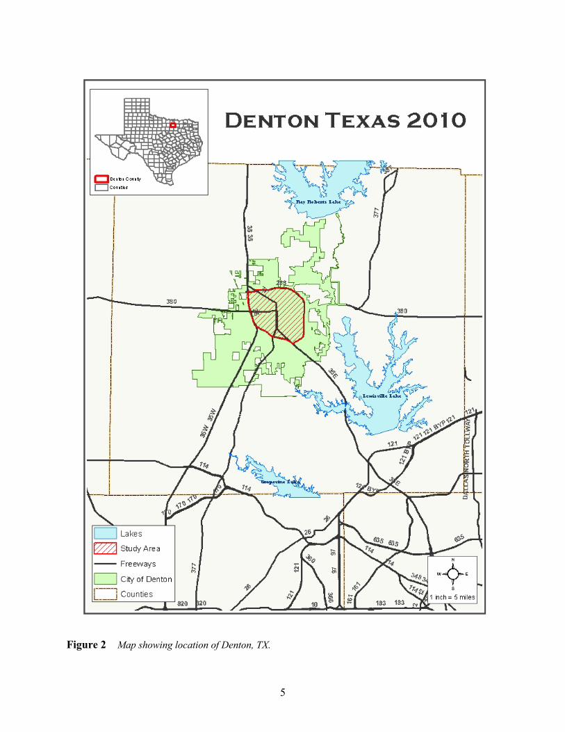
2.1 Denton, Texas
Denton, Texas encompasses an area of roughly 93 square miles and has a population of
over 120,000 with a growth rate at 2 percent per year; it is among the top 25 fastest growing
cities in the nation. The study area is encompassed by the major roads running through the city:
I35 E and Loop 288 and has two primary eco-regions which are the Grand Prairie and Eastern
Cross Timbers. This area provides a good cross section of various soil types and land use classes
as well as many of the local businesses and residences. As of 2010 the study area comprised:
1669 acres of buildings, 685 acres of herbaceous, 4907 acres of mowed/grazed/agricultural, 2783
acres of transportation, 2683 acres of trees and 65 acres of water.
Figure 1 Land use distribution for the study area.
5
Figure 2 Map showing location of Denton, TX.
6
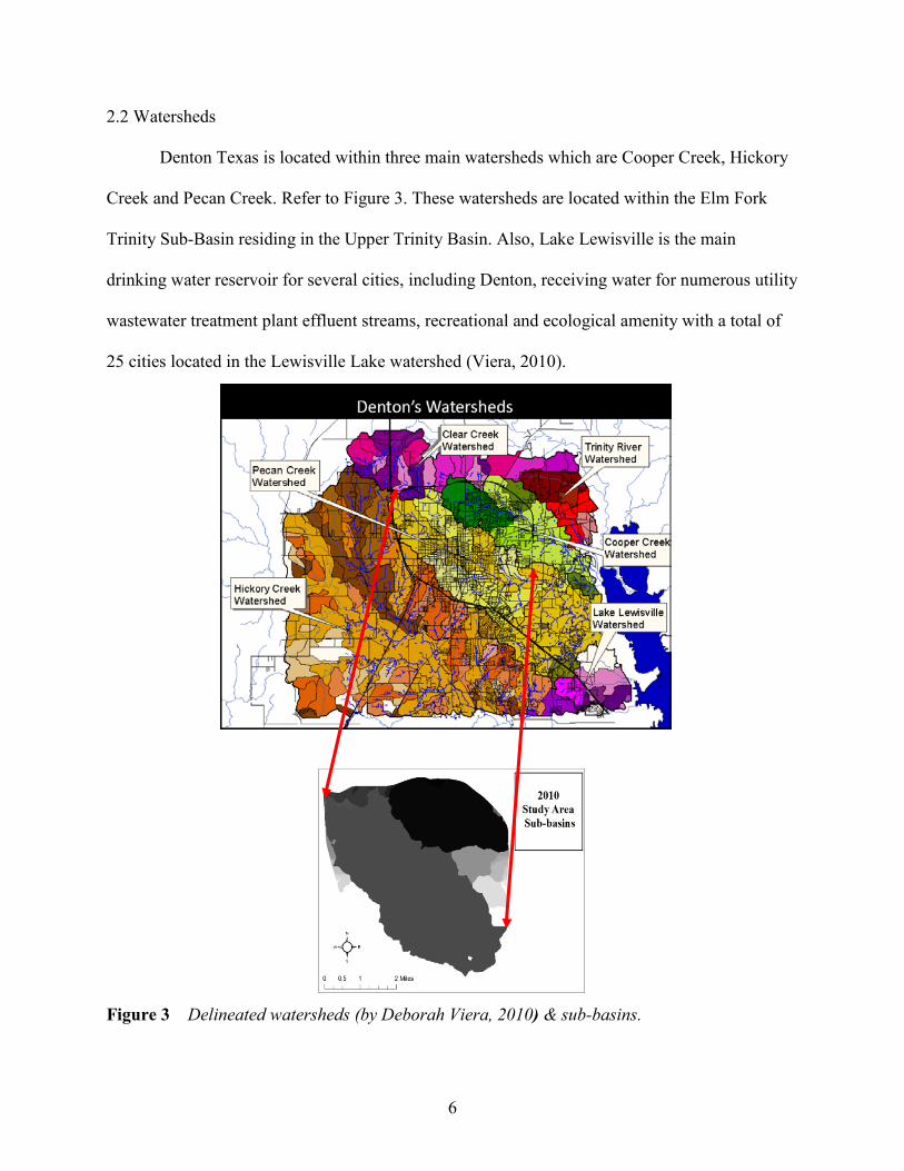
2.2 Watersheds
Denton Texas is located within three main watersheds which are Cooper Creek, Hickory
Creek and Pecan Creek. Refer to Figure 3. These watersheds are located within the Elm Fork
Trinity Sub-Basin residing in the Upper Trinity Basin. Also, Lake Lewisville is the main
drinking water reservoir for several cities, including Denton, receiving water for numerous utility
wastewater treatment plant effluent streams, recreational and ecological amenity with a total of
25 cities located in the Lewisville Lake watershed (Viera, 2010).
Figure 3 Delineated watersheds (by Deborah Viera, 2010) & sub-basins.
7
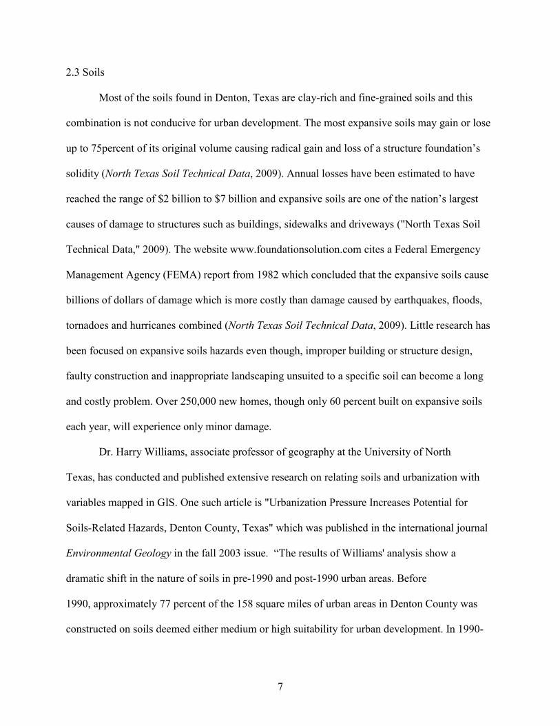
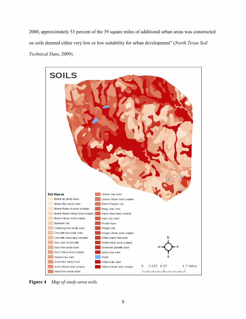
2.3 Soils
Most of the soils found in Denton, Texas are clay-rich and fine-grained soils and this
combination is not conducive for urban development. The most expansive soils may gain or lose
up to 75percent of its original volume causing radical gain and loss of a structure foundation’s
solidity (North Texas Soil Technical Data, 2009). Annual losses have been estimated to have
reached the range of $2 billion to $7 billion and expansive soils are one of the nation’s largest
causes of damage to structures such as buildings, sidewalks and driveways ("North Texas Soil
Technical Data," 2009). The website www.foundationsolution.com cites a Federal Emergency
Management Agency (FEMA) report from 1982 which concluded that the expansive soils cause
billions of dollars of damage which is more costly than damage caused by earthquakes, floods,
tornadoes and hurricanes combined (North Texas Soil Technical Data, 2009). Little research has
been focused on expansive soils hazards even though, improper building or structure design,
faulty construction and inappropriate landscaping unsuited to a specific soil can become a long
and costly problem. Over 250,000 new homes, though only 60 percent built on expansive soils
each year, will experience only minor damage.
Dr. Harry Williams, associate professor of geography at the University of North
Texas, has conducted and published extensive research on relating soils and urbanization with
variables mapped in GIS. One such article is "Urbanization Pressure Increases Potential for
Soils-Related Hazards, Denton County, Texas" which was published in the international journal
Environmental Geology in the fall 2003 issue. “The results of Williams' analysis show a
dramatic shift in the nature of soils in pre-1990 and post-1990 urban areas. Before
1990, approximately 77 percent of the 158 square miles of urban areas in Denton County was
constructed on soils deemed either medium or high suitability for urban development. In 1990-
8
2000, approximately 53 percent of the 39 square miles of additional urban areas was constructed
on soils deemed either very low or low suitability for urban development” (North Texas Soil
Technical Data, 2009).
Figure 4 Map of study-area soils.

9
2.4 Climate
The weather in Denton is typically very hot for the long summer months with
temperatures easily reaching above 100 degrees Fahrenheit. In the winter months the weather is
typically mild and cool with average temperatures ranging from 30-50 degrees Fahrenheit. Rain
is not a common occurrence in this part of North Texas but when it does happen it is mostly in
the spring months of March through June (May being the wettest month) and also in the fall
months of September through October. The average climate and precipitation in Denton was
calculated based on data reported by over 4,000 weather stations and this information was found
at city-data.com. There is a stark difference between the United States average precipitation,
around 3 inches a year, to Denton which can range anywhere from less than 2 inches to over 5
inches. The study area is in a geographic location that consists of random, short bursts of
thunderstorms and heavy precipitation that can produce serious flooding issues due to the
prominently clayey soils and constant urban development. This data highlights the radical and
inconsistent weather patterns that are present in this part of the state. Also, this area of North
Texas is on the southern cusp of the tornado alley corridor which can see tornados through the
spring season on a significantly above state average and 268percent greater than the United
States average level (Stats about All US Cities, 2011).

10
CHAPTER 3
BACKGROUND
3.1 City of Denton Tree Canopy Survey Project
The idea for this paper was spurred from a research contract, which I solely conducted
and was responsible for, through the University of North Texas for the city of Denton Texas to
quantify existing tree canopy for the city and its extra territorial jurisdiction (ETJ). The purpose
of this research was to help arm the city officials with significantly accurate data so they can
better manage their existing tree canopy and make smarter decisions regarding future land
annexations that may or may not contain any tree canopy; as a bonus land use data was also
produced. With problems such as the current economy and decreasing budgets this study will
help municipal managers make tough choices regarding the management of the city’s urban
infrastructure. Urban trees perform a vital service by cleaning the air through sequestering
(through its leaves) and storing pollutants such as carbon monoxide, ozone, nitrogen dioxide,
particulate matter and sulfur dioxide in its biomass. This service affects the well-being of all
urban dwelling citizens and that of the local water quality. Urban trees can prevent erosion,
divert storm water runoff and encourage it to soak into the ground which helps recharge
underground water supplies. All of these natural benefits from trees are quantified and explained
through the analysis of satellite imagery using advanced remote sensing techniques. The city
provided the funding for the satellite imagery and software in this analysis through means that
did not use tax payer money. The money came from a fund that entails all fines imposed on
individuals who illegally cut downs trees, etc; however local citizens and news sources were ill-
informed and did not understand this. As a result there was some initial hesitation and resistance
from a few individuals, but this proves as a prime example of how more than ever it is

11
imperative to step up the education and information sharing to the public; better informed
citizens equals a better managed city.
The remote sensing part of the analysis was accomplished using Definiens eCognition
Developer and the initial segmentation of the image data was a multi-resolution analysis and top-
down system that breaks down the image into super classification groups then subsystems are
created to refine further the details in the image. In this object-based classification, object size,
shape and other parameters can be adjusted to fit the needs of the research. Further, this study
because of the spectral and structural heterogeneity of trees, the nearest neighbor classifier was
be mostly used. Typically the method for classification has been pixel-based in programs such as
Erdas Imagine. Pixel-based classification does not consider the relationship of each pixel data
with its adjacent units. However eCognition takes a more human approach by its ability to filter
out minor inconsistencies and in general streamline the work phase of tree canopy mapping.
When a person looks at an object they subconsciously analyze image properties such as: what
shape is that object, how big is it, what is its color scheme, what is the texture of the object and
also what is surrounding the object. In this case the images were classified into one of the
following classes: trees, buildings, herbaceous, agriculture/mowed/grazed, transportation, bare
land and water. The classification process can become increasingly more complicated so the
amount of subclasses created is entirely dependent on the time period given for the research to be
completed; in this case 8 months. Also, the accuracy rate for this research was established by
field work using a GPS system to map selected areas of tree clustering and other super classes
for comparison. After a proper accuracy rate was achieved the newly created vector shapefile
was further processed using another program called ArcMap.
12
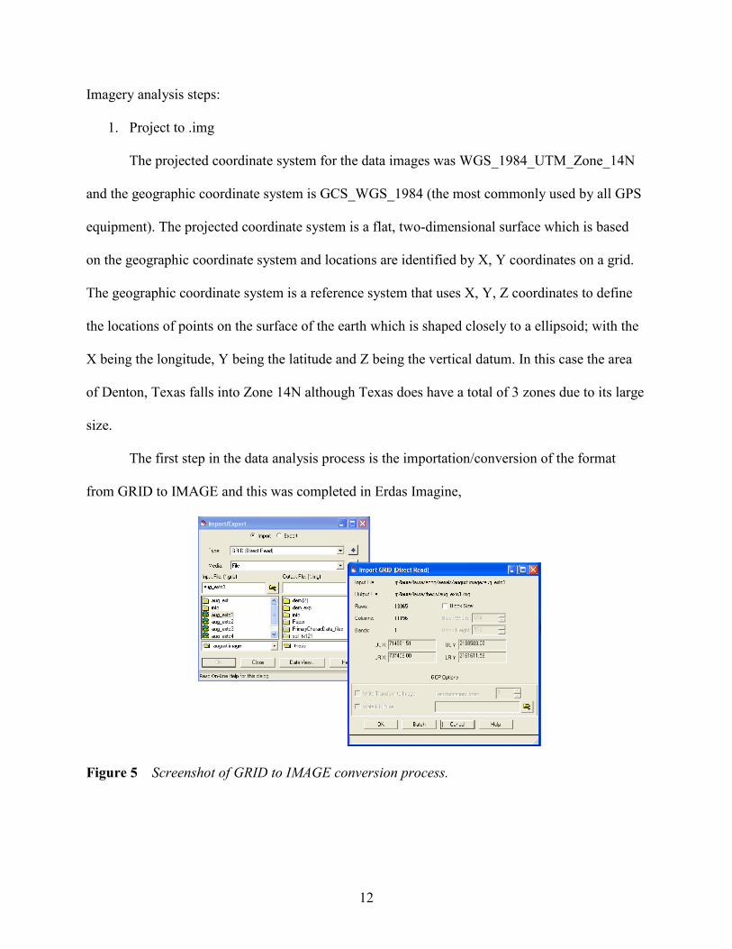
Imagery analysis steps:
1. Project to .img
The projected coordinate system for the data images was WGS_1984_UTM_Zone_14N
and the geographic coordinate system is GCS_WGS_1984 (the most commonly used by all GPS
equipment). The projected coordinate system is a flat, two-dimensional surface which is based
on the geographic coordinate system and locations are identified by X, Y coordinates on a grid.
The geographic coordinate system is a reference system that uses X, Y, Z coordinates to define
the locations of points on the surface of the earth which is shaped closely to a ellipsoid; with the
X being the longitude, Y being the latitude and Z being the vertical datum. In this case the area
of Denton, Texas falls into Zone 14N although Texas does have a total of 3 zones due to its large
size.
The first step in the data analysis process is the importation/conversion of the format
from GRID to IMAGE and this was completed in Erdas Imagine,
Figure 5 Screenshot of GRID to IMAGE conversion process.

13
2. Mosaic Raster
The next step after converting the data to the proper format, .img, is to further prepare it for
analysis. The imagery was delivered as four separate raster’s so a mosaic was performed, in
Erdas Imagine, to create a single raster dataset.
3. Rectify Image: First order polynomial transformation
The satellite imagery was projected as .img (image) files and the next step is to rectify the
imagery; this can be done in the remote sensing software Erdas Imagine. The polynomial model
will be used for this because it is the simplest model and can handle the georeferencing
requirements. A first order polynomial transformation will shift, scale and rotate the raster and it
can be used to rectify scanned maps or satellite images on flat areas. For each of the four satellite
images ground control points (GCP’s) were collected and used to transform the raster to map
coordinates. Viewer 1 contained the satellite image and Viewer 2 contained the roads and
streams shapefile for the City of Denton. The shapefiles were obtained by the NCTCOG DFW
Clearinghouse website that provides free data to the public. The shapefiles being used as a
reference to rectify the images has a projected coordinate system called
NAD_1983_StatePlane_Texas_North_Central_FIPS_4202_feet but they were converted to
match the images geographic coordinate system GCS_WGS_1984.
As the last part of the rectification process the four images were resampled to the
coordinate system of the shapefiles. In Erdas Imagine there is a tool in the Data Preparation
category that can re-project the images; note that the units for this projection will be in meters.
Also the resample method of Nearest Neighbor was chosen because it assigns to each pixel the
value of its nearest neighbor in the new coordinate system. It is the fastest re-sampling technique
and is appropriate for thematic data; it’s also the easiest and fastest method of interpolation. The

14
shapefiles will have to be re-projected from the NCTCOG so they would match the coordinate
system of the imagery. The Geographic Transformation of NAD_1983 to WGS_1984 with the
zone of 4 will be applied because the State Plane coordinate system is based in Feet and not
Meters like WGS_UTM. This is an example of one of the over 400 types of projection systems
available. Roughly 30-100 data points were referenced, with 3 ground control points, from
Viewer 1 to Viewer 2 in Erdas, based on road-road and stream-road intersections. These
reference and index points were saved as files separate from each other. The goal was to get as
many reference points as possible with the Root Mean Square (RMS) error of each point to be
5.0 or less.
The degree of which the transformation can accurately map all control points can be
measured mathematically by comparing the actual location of the map coordinate to the
transformed position in the raster. The distance between these two points is known as residual
error. This value describes how consistent the transformation is between the different control
points and after deleting the points exceeding this value, of 5.0, I was left with only 10-20
reference points on average. No matter how many reference points you start out with there is
always a chance that more than half of them will be deleted. In the rectification the output cell
size was set to 2.0 by 2.0 because the image was originally 2 meter in resolution.
4. Pan Sharpen
5. Dice Image into tiles 6. Create NDVI layer
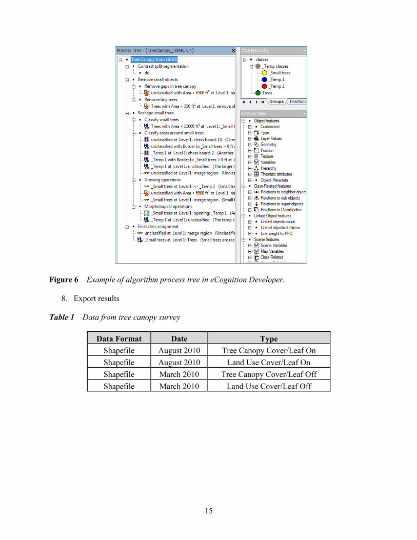
7. Classify images using factors such as shape, size, color, texture, height etc.
15
Figure 6 Example of algorithm process tree in eCognition Developer.
8. Export results Table 1 Data from tree canopy survey
Data Format Date Type Shapefile August 2010 Tree Canopy Cover/Leaf On Shapefile August 2010 Land Use Cover/Leaf On Shapefile March 2010 Tree Canopy Cover/Leaf Off Shapefile March 2010 Land Use Cover/Leaf Off

16
Figure 7 Denton city & ETJ tree canopy cCover.
Ultimately trees and other green infrastructure in a community can solve many problems,
such as flood prevention and increased water quality, through their natural services. This makes
it imperative to have a baseline dataset from which to plan future projects, such as urban
expansion, and fix current problematic areas. An example of this would be planting more trees
around oil and gas well sites that are close to streams so water quality can be improved. This
study will not only benefit the citizens of Denton but it will also not cost them a dime in tax
payer’s money. By putting a realistic monetary value (typically hundreds of thousands of dollars)
on the natural functions of tree’s city officials can make better informed decisions; also local
citizens will potentially better understand the importance of the tree canopy to the community as
a whole. The resulting data sets of the Tree Canopy Survey, of which I solely conducted, were
used as variables in this research paper. The land use data was implemented in the storm water
runoff model to represent Denton in the year of 2010.

17
Figure 8 Denton city & ETJ 2010 land use.
Figure 9 Study area 2010 land use.

18
3.2 Storm Water Models
Table 2 Characteristics of urban rainfall-runoff models
3.2.1 Screening Models
Screening models are preliminary, “first-cut”, desktop procedures that do not require the
use of a computer. Their goal is to provide a first estimate of the magnitude of urban runoff
quantity and quality problems before an investment of time and resources into more complex
computer based models. Only after the screening model indicates its necessity should one of the
latter models be used (United States of America, 1992).
A very popular example of a screening model is the HSSM (hydrocarbon spill screening
model) developed by the EPA which stimulates subsurface releases of light non-aqueous phase
liquids. When it comes to hydrocarbon spills, there is no other model as powerful and versatile as

19
HSSM (Scientific Software Group, 2005). The Hydrocarbon Spill Screening Model serves as a
simplified model for subsurface releases of fuel hydrocarbons and the most common problem
that the model may be used to address is that of a leaking underground storage tank. “As of the
end of 1997, there have been over 400,000 confirmed releases from underground storage tanks in
the U.S. (“The Hydrocarbon Spill Screening Model,” 2011).
The EPA states that for subsurface contamination, the most important characteristics of
fuel hydrocarbons are that they are: immiscible with water (oil and water don't mix), less dense
than water, composed of chemicals that have varying water solubility’s and volatilities and
composed of a number of chemicals that can have adverse health effects. This model was applied
to a study done by James W. Weaver of the American Society of Civil Engineers in which field
data from two case histories were used to develop input parameter sets for HSSM. In one case
there was aqueous concentration data from an extensive monitoring network and in the second
case the monitoring network was small, but the date and volume of the release could be
estimated. The cases were chosen because they both have features that were well suited for
testing of the model. In both cases the model was able to reproduce the trends in the data set and
the concentrations to within an order of magnitude (Weaver, 1996).
3.2.2 Planning (Continuous) Models
Another type of model is planning which is used for an overall assessment of the urban
runoff problem. It is also utilized for estimates of the effectiveness and costs of abatement
procedures. These models are recognized by the relatively large time steps (hours) and long
simulation times (months and years), i.e., continuous simulation; data requirements are kept to a
minimum and their mathematical complexity is low. They may also be run to identify hydrologic

20
events that may be of special interest for design or other purposes (United States of America,
1992).
The paper “A Case in Support of Continuous Modeling for Stormwater Management
System Design” describes a case study in the Town of Milton (Sixteen Mile Creek Watershed) in
which two methods, Design and Continuous, were applied in the analysis and preliminary design
of end-of-pipe storm water management facilities. It was found that the Design approach tended
to over-estimate antecedent moisture conditions for existing land use conditions, and the
subsequent peak runoff which defines the target flows. Also this approach does not provide
sufficient control for the more frequent storm events and does not provide an effective means for
designing erosion control. The continuous modeling approach resulted in less overall storage
than the Design approach and requires substantial amounts of reliable data for proper calibration
and simulation. The results of this case study demonstrates that the continuous modeling
approach was most appropriate for the Sixteen Mile Creek, Areas 2 and 7 Sub watershed
Planning Study, the design approach could be considered for smaller catchments and local storm
water management system design verification (Ferrell et al, 2001).
Another continuous model is Version 5 of the SWMM got Microsoft Windows and it is a
freeware program. This model creates a continuous simulation using historical rainfall series and
was used in the long-term modeling of the urban area of Lisbon. The continuous modeling
allowed for the comparison of benefits of different scenarios of storage and sewage treatment
plant capacities for the reduction of the overflow discharges. Also, in addition to increases in
difficulties and uncertainties associated to the water quality model, there were no relevant
benefits obtained by its use. It was concluded that some limitations were found such as only a
maximum of about thirty days data could be loaded to SWMM5 from a 2-minute interval inflow

21
time series; this limitation is considerably minimized with the introduction of rainfall time series
(Cambez et al, 2008).
The hourly precipitation time-series is a previous common practice that used the nearest
precipitation gauge while the new and future practice of this model utilizes an extended
precipitation time-series. To calculate the precipitation time-series you use the nearest hourly
gauge and multiply all hourly values by a single scaling factor. The scaling factor is the ration of
25-year 24-hour precipitation at the site of interest relative to the gage. An MGS Flood
Continuous Flow Model for Storm water Facility Design training workshop was put on by MGS
Engineering Consultants Inc. in Olympia, Washington. A major issue that arose with the use of
the Simple Scaling model was that the nearest gage may not have representative records for
various reasons. It is not possible to rescale the time-series with a single scaling factor and
manage to obtain the correct storm characteristics at all durations at the site of interest; storm
characteristics could vary by the season and duration. Finally many gages have short record
lengths making it impossible to use for the intended design purposes. To compensate for the
shortcomings of this model they created an extended precipitation time-series. Essentially a long
precipitation record was created by combining obtained records from distant gage stations.
Records from each station were rescaled to have storm statistics representative of the site of
interest. In the workshop they combined the precipitation data records for: Vancouver, BC (38
years), Seattle, WA (60 years) and Salem, OR (60 years). In the end this allows for the use of
high-quality stations with long records and avoids the pot-luck of using nearby stations. It seems
that many hourly stations have short records of poor-quality so this will provide greater diversity
and variability of storm temporal patterns and provides for greater sampling of storm magnitudes
and temporal patterns (Schaefer et al, 2002).

22
3.2.3 Design Models
Event-based models are often preferred to continuous models for real time operational
applications and forecasting in combination with radar spatial rainfall. The response of a
catchment to a rainfall event is greatly influenced by the antecedent soil moisture conditions,
which are crucial parameters for flood models like design models. They are typically used to
simulate of a single storm event and which will provide a description of flow and pollutant
routing. This begins from the point of rainfall through the entire urban runoff system are a highly
useful tool for both water quantity and quality problems in urban areas. The data requirements
may be moderate to very extensive depending upon the specific model employed and it is
characterized by short time steps (minutes) and short simulation. The EPA storm water
management model (SWMM) is dynamic in rainfall-runoff simulation and is used for single
event or long-term (continuous) simulation of runoff quantity and quality from primarily urban
areas. The runoff component operates from a collection of subcatchment area; rain falls and
runoff is generated there. The routing part of the model will move the runoff through a
conveyance system of pipes, channels, storage/treatment devices, pumps, and regulators; flow
rate, flow depth, and quality of water in a simulation period are comprised of multiple time steps.
This computer model has changed significantly since it was first developed in 1971 and the
current is Version 5 (Rossman, 2011).
Hydrologic processes accounted for in SWMM: time-varying rainfall, evaporation of
standing surface water, snow accumulation and melting, rainfall interception from depression
storage, infiltration of rainfall into unsaturated soil layers, percolation of infiltrated water into
groundwater layers, interflow between groundwater and the drainage system, nonlinear reservoir
routing of overland flow and even runoff reduction via low impact development (LID) controls

23
(Rossman, 2011). By dividing the study area into a collection of smaller, replicate subcatchment
areas, each containing its own fraction of pervious and impervious sub-areas, the spatial
variability can be achieved.
3.2.4 Other Models
There are many different types and applications of urban stormwater runoff models.
Some other models include the operational model which is used to produce actual control
decisions during a storm event. It works through the introduction of rainfall from telemetered
stations and is used to predict system responses a short time into the future. Models are
frequently being developed from more sophisticated design models and modified to be applied in
a specific system. There are also many more models are available for purely hydrologic and
hydraulic analysis.
3.2.5 Simple Model: SCS Runoff Curve Number Method
This model was chosen for use in this research paper because it is simple and based on a
study area's hydrologic soil group, land use, treatment and hydrologic conditions. However a
drawback to this method is that it will not calculate when the runoff will occur during the
precipitation event. If the exact time of the runoff is also desired then you will have to introduce
a time-of-concentration method, such as the lag method, to calculate it.
The runoff curve number method (RCN) was a method originally established by the
Soils Conservation Society in 1954 and was initially designed to be an inter-agency tool for
runoff estimation on agricultural fields. It has been adapted over the years within the urban
hydrology community and become the most recognized method for computing peak runoff rates
and volumes. Technical Release 55 (TR-55) was created to be a simplified NRCS tool for the

24
computation of runoff rates that joins the NRCS runoff equation with unit hydrograph theory
(Schiariti, n.d.). The higher the CN value the higher the potential will be for runoff and flooding.
The runoff equation is
Where
Q is runoff ([L]; in) P is rainfall ([L]; in) S is the potential maximum soil moisture retention after runoff begins ([L]; in) Ia is the initial abstraction ([L]; in), or the amount of water before runoff, such as infiltration, or rainfall interception by vegetation; and it is generally assumed that Ia = 0.2S
The runoff curve number, CN, is then related
Lower CN numbers indicate low runoff potential while larger numbers are for increasing runoff
potential. The lower the curve number, the more permeable the soil is.
25
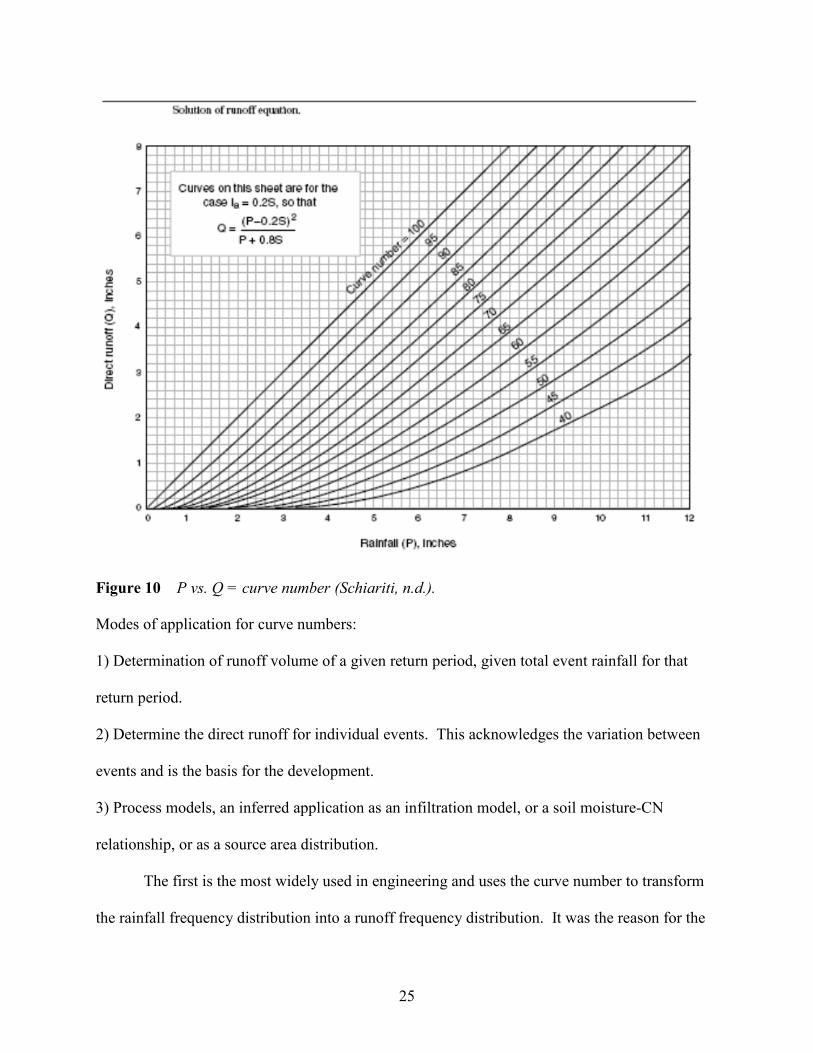
Figure 10 P vs. Q = curve number (Schiariti, n.d.).
Modes of application for curve numbers:
1) Determination of runoff volume of a given return period, given total event rainfall for that
return period.
2) Determine the direct runoff for individual events. This acknowledges the variation between
events and is the basis for the development.
3) Process models, an inferred application as an infiltration model, or a soil moisture-CN
relationship, or as a source area distribution.
The first is the most widely used in engineering and uses the curve number to transform
the rainfall frequency distribution into a runoff frequency distribution. It was the reason for the

26
development of the model. The runoff volume that is computed is often overlooked and the peak
discharge, which is more frequently the desired value, calculated with a unit hydrograph model
and used directly. The second mode of application is the basis for the original development and
there is a wide variation of runoff from rainfalls of the same magnitude. This forces the
realization that CN can vary between storms for many different reasons. The curve number
model could potentially be seen as an infiltration model. This is because in its application it is
used to determine runoff incrementally over the duration of the storm for input into a unit
hydrograph model.
The antecedent moisture condition (AMC) is the preceding relative moisture of surfaces
before a rainfall event and it comes in three different levels: AMC I, AMC II and AMC III. For
this model we will consider the watershed to be in an AMC II state which is an average moisture
condition. This is important to understand because if the conditions of pervious surfaces are very
dry (AMC I condition) before a rainfall event it could affect the modeled results significantly; as
well as a pre-existing AMC III condition (considerable preceding rainfall prior).
Table 3 CN look-up table created from combined soils & land use grids
NRCS Cover Type A My Cover Types Hydrologic Condition A B C D
Herbaceous—mixture of grass, Herbaceous Poor 67 80 87 93 Paved; curbs and storm drains (excluding
right-of-way) Transportation 98 98 98 98
Pasture, grassland, or range-continuous forage for grazing
Agriculture, Mowed & Grazed
Poor 68 79 86 89
Fair 49 69 79 84
Good 39 61 74 80
Woods – grass combination (orchard or tree farm) Tree Canopy
Poor 57 73 82 86
Fair 43 65 76 82
Good 32 58 72 79 Paved parking lots, roofs, driveways, etc.
(excluding right-of-way) Buildings 98 98 98 98

27
3.3 Remote Sensing and GIS Techniques
“Remote sensing is the observation and measurement of objects from a distance, i.e.
instruments or recorders are not in direct contact with objects under investigation” (Aber et al.,
2002). There are four types of resolutions that contribute to the quality of the data: spatial,
spectral, radiometric and temporal:
• Spatial resolution: pixel size recorded in a raster image (usually in meters)
• Spectral resolution: wavelength width of different band frequencies; Landsat has seven
bands plus many from the infra-red spectrum, spectral resolution range of 0.07 to 2.1 µm
• Radiometric resolution: number of different intensities of radiation the sensor can detect
and distinguish, range from 8 to 14 bits, 256 levels of gray scale and up to 16,384
intensities of color in each band
• Temporal resolution: frequency of flyovers by a satellite or plane, cloud cover makes it
necessary to do multiple flyovers, only relevant in time-series studies or if averaged or
mosaic image is required.
There are several remote sensing techniques and they are based on sensing
electromagnetic energy that is emitted (or reflected) from the surface of the Earth which is then
detected from an altitude high above the ground. There are two types of remote sensing:
Passive: Detect available electromagnetic energy from naturally occurring sources such as
sunlight. It is based on two energy sources.
1. Ultraviolet, visible, and near-infrared radiations (< 3 µm wavelength) are mainly
reflected solar energy.
2. Mid-infrared, thermal-infrared, and microwave radiations (> 3 µm wavelength) are
mostly emitted from the Earth's surface

28
Active: Utilizes an artificial "light" source, such as radar, to illuminate the scene.
There are three main types of remote sensing (Aber et al., 2002):
1. Aerial photography
a. Spectral sensitivity: 0.3 µm (near-ultraviolet) to 0.9 µm (near infrared)
b. Photographs taken in b/w panchromatic, b/w infrared, color-visible, color-
infrared, and multiband types
c. Equipment: airplanes or helicopters
d. Useful in fields such: archeology, biology (habitat, wildlife census), forestry,
geology, geomorphology, engineering, hydrology, mineral and oil prospecting,
pollution (air, land, water), transportation or even urban planning
2. Manned-space photography
a. Spectral response range: 0.4 to 1.1 µm
3. Landsat satellite imagery:
a. Advantages: “(1) Synoptic view: Satellite images are "big-picture" views of large
areas of the surface. The positions, distribution, and spatial relationships of
features are clearly evident; mega patterns within landscapes, seascapes, and
icescapes are emphasized. Major biologic, tectonic, hydrologic, and geomorphic
factors stand out distinctly. (2) Repetitive coverage: Repeated images of the same
regions, taken at regular intervals over periods of days, years, and decades,
provide data bases for recognizing and measuring environmental changes. This is
crucial for understanding where, when, and how the modern environment is
changing. (3) Multispectral data: Satellite sensors are designed to operate in many
different portions of the electromagnetic spectrum. Ultraviolet, visible, infrared,

29
and microwave energy coming from the Earth's surface or atmosphere contain a
wealth of information about material composition and physical conditions. (4)
Low-cost data: Near-global, repetitive collection of data is far cheaper using
satellite sensors than collecting the same type and quantity of data would be
through conventional ground surveys” (Aber et al., 2002).
b. Landsat Series of 1970s, 80s and 90s: Multispectral Scanner (MSS) – (1)
Moderate-resolution scanner, collected data in four spectral bands: green, red, and
two near-infrared channels. Pixel size in processed datasets is 57 m by 57 m. (2)
Thematic Mapper (TM) -- An advanced high-resolution scanner that collects
spectral data in seven bands: blue, green, red, near-infrared, two mid-infrared, and
thermal-infrared. Pixel size in processed datasets is 28½ m by 28½ m. For more
information--see Landsat TM (Aber et al., 2002).
Raster images are collections of pixels, which can be thought of as small squares in a
very fine grid. Each pixel is associated with information on color value and intensity for that
portion of the grid. Images in vector format are in the form of points, lines, and closed figures
called polygons. Points are described by coordinates and the positions, directions, and shapes of
lines are described by geometric and mathematical relationships. This is important to consider
because ideally photographs should be taken midday to have less shadowing and provides for
easier interpretation. Photo interpretation is also subject to classification errors/misclassification
of the image. For example, tree shadows can be erroneously included as tree canopy or shrubs
may be mistakenly classified as trees. Classification errors can lead to consistent overestimates
or underestimates of canopy cover but it is simply another factor that must be taken into
consideration when spending such a large amount of money on data and analysis. Digital image

30
analysis can also be used to create permanent maps that may be incorporated into a geographic
information system and be used to show how and where land use changes occur over time. If
data will be used for these other purposes and future monitoring then the additional cost of
digitizing a city’s land use can be justified. Digital image analysis techniques have the potential
to provide precise estimates of objects such as tree canopy cover (Swiecki et al., 2001). Also, it
is made possible to collect data for dangerous areas that cannot be accessed or large areas that
make it impossible to cover on foot.
In most types of imagery, items of interest are typically represented as a collection of
pixels that vary in color and/or intensity. Image analysis software uses a variety of techniques to
convert an image into a series of monochromatic layers, each of which represents a single type of
feature. One widely used and accepted software program currently being used throughout many
universities, organizations and businesses worldwide is Erdas Imagine. Erdas Imagine is a
geospatial raster data processing application that lets the user prepare data for mapping in areas
such as GIS. This software is pixel based classification with the pixel reflectance from surfaces
in the image mainly being used as the major classification parameter. This software is used for
many different types of analysis including vegetation analysis, linear feature extraction,
generation of processing work flows, import/export of data for a wide variety of formats and
mosaicing of imagery. The two main benefits of this software package are: 1. it is relatively easy
to learn on the fly and 2. The results from the software is universally accepted and respected.
Erdas uses unsupervised, supervised or knowledge-based classification while eCognition uses
segmentation and object-oriented classification. Definiens eCognition implements the process of
how a person identifies objects with their brain and transfers it into an algorithm building
application. A hierarchical network of segments in different scale levels is built while also
31
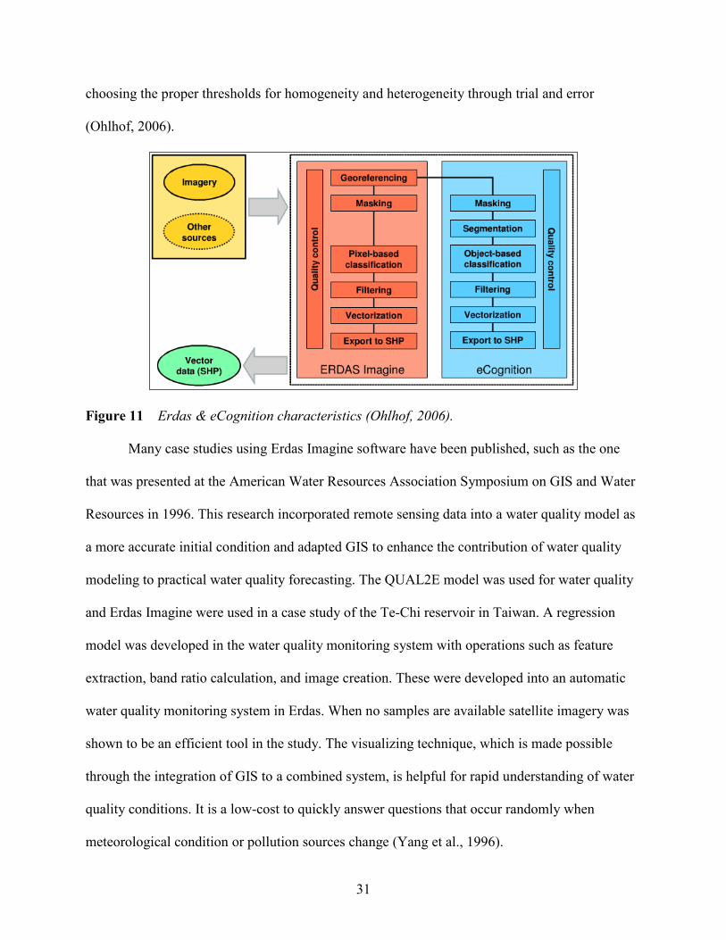
choosing the proper thresholds for homogeneity and heterogeneity through trial and error
(Ohlhof, 2006).
Figure 11 Erdas & eCognition characteristics (Ohlhof, 2006).
Many case studies using Erdas Imagine software have been published, such as the one
that was presented at the American Water Resources Association Symposium on GIS and Water
Resources in 1996. This research incorporated remote sensing data into a water quality model as
a more accurate initial condition and adapted GIS to enhance the contribution of water quality
modeling to practical water quality forecasting. The QUAL2E model was used for water quality
and Erdas Imagine were used in a case study of the Te-Chi reservoir in Taiwan. A regression
model was developed in the water quality monitoring system with operations such as feature
extraction, band ratio calculation, and image creation. These were developed into an automatic
water quality monitoring system in Erdas. When no samples are available satellite imagery was
shown to be an efficient tool in the study. The visualizing technique, which is made possible
through the integration of GIS to a combined system, is helpful for rapid understanding of water
quality conditions. It is a low-cost to quickly answer questions that occur randomly when
meteorological condition or pollution sources change (Yang et al., 1996).
32
ERDAS is used frequently in digital photogrammetry so it is important for the accuracy
to be assessed when aerial triangulation is carried out. The goal of aerial triangulation (AT) is to
connect and increase ground control points through strip and/or block for other photogrammetric
applications. In a study by the Faculty of Geoinformation Science & Engineering at the
University Teknologi Malaysia, AT was performed based on one strip of photograph and a block
of photograph. The study area is the community area encompassing University Teknologi
Malaysia main campus in Johor Bahru. ERDAS assessed the accuracy of aerial triangulation
based on a strip or block of aerial photographs and the results obtained from both the quantitative
and qualitative analysis lead to the deduction that the aerial triangulation process in ERDAS
software is fairly accurate for both strip and block aerial photographs. However it was also
suggested in the RMSE (root mean square estimate) that the accuracy obtained from a strip of
aerial photography is slightly higher than that obtained from the block of photographs. Some
debate was brought up on how much control would be adequate for a given area to reach
saturation; some suggest 25 to 30 or even up to 35 ground control points (Bisher et al., 2010).
The City of Fayetteville, Arkansas realized in 2003 that there was a need to rapidly and
inexpensively generate an accurate, up-to-date map of impermeable surfaces within the city’s
utility service area. This area covers approximately 170 square miles in and around Fayetteville,
Arkansas. Definiens eCognition was chosen for this project and was completed using the nearest-
neighbor algorithm. Spectral values in the raw data, land-use information derived from Landsat 7
imagery, proximity to known buildings and roads, object size and border information were a
number of spatial characteristics taken into account during the analysis. To obtain the high
spatial/positional accuracies, the impervious surface maps were extracted from high resolution,
ortho-corrected satellite imagery. These ortho-images were derived from Digital Globe’s

33
Quickbird Standard Ortho-Ready image product. The “standard” Quickbird product was
augmented using existing control point data supplemented with additional sub-meter GPS
observations, and a 10 foot DEM provided by city of Fayetteville. The final map product was in
the form of a five category map suitable for storm water management modeling. The categories
are: impervious surface, forest/wooded, grasses/herbaceous, exposed soils, and water. Accuracies
were determined based upon ground-truth points collected at times roughly corresponding to the
image acquisition with overall accuracy for the map at 84.21percent (University of Arkansas,
2003).
Geographic information systems have been applied as a modeling tool for years because
engineers use it to run hydrologic models such as the HEC-1 and HEC-2. This inherently
supports the dynamic task of basin master planning because engineers are now finding ways to
use GIS more and more. When data is made available in GIS, it can be extracted and/or
combined with other data which can essentially be reformatted for various modeling processes
and used to generate other inputs needed by the models. Another benefit of using GIS is that it
can also be used to ensure data has been collected correctly (Robbins et al., 1999). Customized
GIS technology will allow the city to organize its stormwater infrastructure and drainage system
maintenance. Advanced technology as well as clear objectives and goals can allow for the
evolution of better plans for urban stormwater management, watershed protection, and watershed
restoration.
Typical applications of GIS for stormwater systems include (Shamsi, 2002):
• Watershed stormwater management
• Planning: assessment of the feasibility and impact of system expansion
• Floodplain mapping and flood hazard management

34
• Mapping work for Stormwater National Pollution and Discharge Elimination System
(NPDES) permit requirements
• Hydrologic and hydraulic (H&H) modeling of combined and storm sewer systems,
including: automatic delineation of watersheds, model simplification, estimating surface
elevation and slope from digital elevation model (DEM) data & also estimating
stormwater runoff from the physical characteristics of the watershed such as land use,
soil, surface imperviousness, and slope
• Documenting field work, including: work order management and inspection and
maintenance of stormwater system infrastructure
Essentially GIS is the combination of cartography, statistical analysis
and database technology resulting in software packages such as the most widely known ArcGIS
by ESRI. These software packages are capable of managing most data types as long as they
contain a geographical component. GIS will be used for a variety of reasons throughout many
different steps of this research, such as preparing the shapefiles containing the land use and soil
data by clipping them to the study area. It will be used for running various calculations between
raster datasets to obtain curve numbers, which will be accomplished by joining a curve number
look up table to the combined land use and soils dataset. Also, GIS will be used to import GPS
data collected to evaluate land use data accuracy through ground control points as well as to
make specialized maps for visual representation of the different analyses outputs.
3.4 Technological Methods and Progress
When it comes to the progress of geography research philosophies, which ultimately
determines the scientific methodology of the research, there is no single recommendation as to
how science should be practiced. John Losee said it best with “Theories of science may be

35
advanced as descriptive generalizations or as prescriptive recommendations about how science
ought to be conducted.” (Losee, 2004) There is some debate, however, about what a research
philosophy actually is.
An important beginning step the scientific research process is identifying between an
extensive and an intensive approach to data collection. Extensive research means that there will
be a large sample of data collected which can then possibly be applied to conclude
generalizations about a trend. This approach has some issues with it such as it is not necessarily
good for actually explaining why something is the way it is. An intensive approach is a more
small data sample/case study-based in that its goal is to actually explain a process either social or
physical. It is important to note that sometimes studies do include both the extensive and
intensive approach. This first step will help to define the actual research philosophy that leads to
the methodological approaches and methods.
The overall applied method for this scientific research is based heavily on the realism
philosophy. There is a triangulation of data sampling, collection and analysis methods in my
research. It combines both subjectivity and objectivity because my form of data interpretation is
heavily subjective due to the high involvement by the researcher. It is somewhat objective in the
sense that the model will be built using data collected, such as elevation data, and mathematical
equations which cannot be interpreted. The research is also deductive in nature because I am
starting out with a hypothesis which will then be tested by the creation and analysis of data. It
will also be quantitatively method-based and it will seek to treat the case as one of an exploratory
nature. This was all based on the type of system my research target fell into which is that of an
open system.

36
“A system is an object of study which is a collection of components, many of which are
related to each other; that is, the components will often be coupled or interact with each other in
various ways” (Wilson, 1981). The area outside of the system is known as its environment. There
are two basic types of research which is categorized based on which system they are in; a closed
system or an open system. A closed is isolated so that it cannot exchange matter or energy with
its surroundings and can therefore attain a state of thermodynamic equilibrium. An open system
transfers both matter and energy across its boundary to the surrounding environment; most
ecosystems open. This research project is just a snapshot of what could actually be developed in
understanding storm water runoff patterns and ways to prevent it.

37
CHAPTER 4
MATERIALS AND METHODOLOGY
4.1 Data
The data used in this study came from two distinct sources: 2-m spatial resolution rectified
satellite images from February and July of 2010 and road, cities, lakes& streams shapefiles
downloaded from the NCTCOG website in March of 2010. IKONOS is a commercial earth
observation satellite, and was the first to collect publicly available high-resolution imagery at 1-
and 4-meter resolution. This satellite offers multispectral (MS) and panchromatic (PAN) imagery
however the new GeoEye-1 satellite bests IKONOS in quality, which is what was used in this
research. The city of Denton purchased the imagery from the company GeoEye. GeoEye made
history with the Sept. 6, 2008 launch of GeoEye-1—the world's highest resolution commercial
earth-imaging satellite. It is equipped with the most sophisticated technology ever used in a
commercial satellite system. It offers unprecedented spatial resolution by simultaneously
acquiring 0.41-meter panchromatic and 1.65-meter multispectral imagery. The detail and
geospatial accuracy of GeoEye-1 imagery further expands applications for satellite imagery in
every commercial and government market sector (GeoEye, 2011).
Table 4 Satellite imagery information
Band Count 4 & 1
Type R, G, B, NIR & Panchromatic
Pixel Size 2 & 0.5
Map Units Meters
Sensor Name GeoEye-1
Processing Level Standard Geometrically Corrected
Image Type PAN/MSI
Interpolation Method Cubic Convolution

38
The data for the 2000 and 2005 Table 5 NCTCOG land use code descriptions
land use surveys came directly from the
north central Texas council of
governments website. The NCTCOG data
had to be prepared before the storm water
analysis because the land classifications
differed from the 2010 classifications I
personally derived during the remote
sensing part of this research. As this paper
does not necessarily care about whom or
how specifics such as buildings are used
(ex: single family homes vs. multi-family
homes) the land use classes are simplified
to match the classes produced from the
2010 survey. This paper only cares about
how each pixel affects storm water runoff
and by consolidating classes the results
and interpretations will be stream lined
and easier to understand. Table 5 to the
right was obtained from the NCTCOG
website and it shows how the
classifications are broken down in the
attribute table and also provides an
39
example of possible uses. For this research the following shows how each LUCODE was
integrated into the 2010 land use classes
Buildings: 111,112,113, 114, 121, 122, 123, 124, 131, 143, 147, 160
Transportation: 141, 142, 144, 145, 146, 173, 306 & 308
Mowed/Grazed/Agricultural: 171, 172
Herbaceous: 300
Water: 500
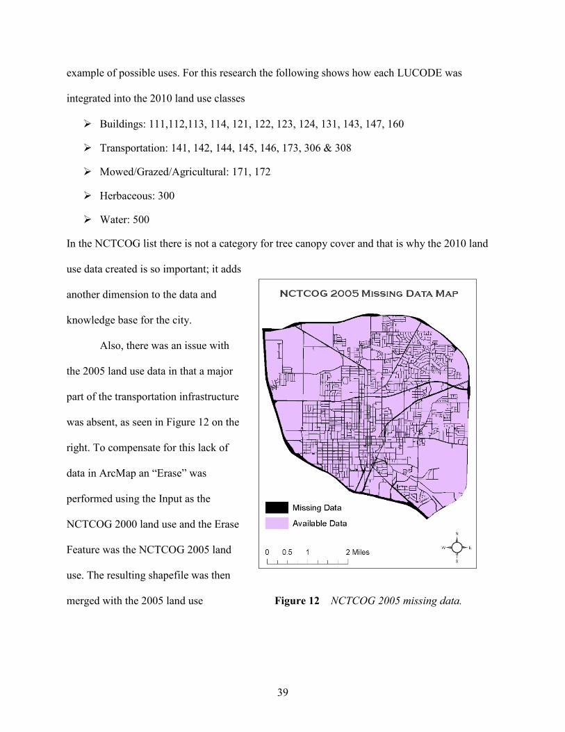
In the NCTCOG list there is not a category for tree canopy cover and that is why the 2010 land
use data created is so important; it adds
another dimension to the data and
knowledge base for the city.
Also, there was an issue with
the 2005 land use data in that a major
part of the transportation infrastructure
was absent, as seen in Figure 12 on the
right. To compensate for this lack of
data in ArcMap an “Erase” was
performed using the Input as the
NCTCOG 2000 land use and the Erase
Feature was the NCTCOG 2005 land
use. The resulting shapefile was then
merged with the 2005 land use Figure 12 NCTCOG 2005 missing data.

40
shapefile in an editing session in ArcMap to fill in the blanks and ensure the cohesiveness of the
data. However after the merging of the 2000 and 2005 data there was still small spots of missing
data which can clearly be seen, so despite efforts to smooth the data there is still some errors.
4.2 Geographic Information Systems Method
Figure 13 Flowchart for storm water runoff analysis.
The implementation of a storm water runoff model is a process which initially starts with
the collection and thorough understanding of the type of data available and how it could be
applied. Surface runoff as well as infiltration was calculated using the land-use data produced
from the remote sensing analysis along with the digital elevation model (DEM), hydrologic soil
condition of AMCII and soil data. “There has been a vast increase in basic soils property data
since Musgrave first proposed the concept of hydrologic soil groups in Handbook of Agriculture
(USDA 1955)” (Van Mullem et al., 2004).
The first step in the Figure 13 flowchart is to take the prepared soil data, which was
clipped to match the study area in ArcGIS, and designate the hydrologic soils groups based on
each polygon’s soil type.
41
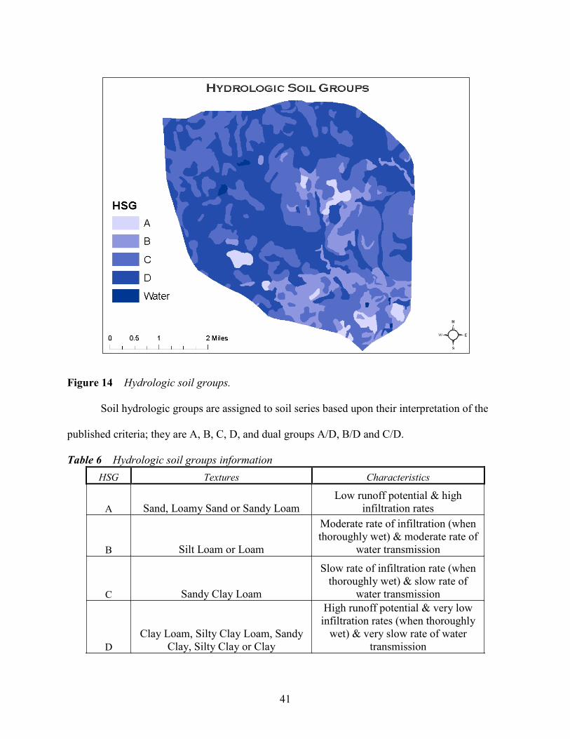
Figure 14 Hydrologic soil groups.
Soil hydrologic groups are assigned to soil series based upon their interpretation of the
published criteria; they are A, B, C, D, and dual groups A/D, B/D and C/D.
Table 6 Hydrologic soil groups information HSG Textures Characteristics
A Sand, Loamy Sand or Sandy Loam Low runoff potential & high
infiltration rates
B Silt Loam or Loam
Moderate rate of infiltration (when thoroughly wet) & moderate rate of
water transmission
C Sandy Clay Loam
Slow rate of infiltration rate (when thoroughly wet) & slow rate of
water transmission
D Clay Loam, Silty Clay Loam, Sandy
Clay, Silty Clay or Clay
High runoff potential & very low infiltration rates (when thoroughly
wet) & very slow rate of water transmission

42
Dual hydrologic soil groups (A/D, B/D, and C/D): some wet soils that could be
adequately drained. The first letter applies to the drained and the second to the un-drained
condition. The table below shows what the curve numbers will look like for different
combinations of land use and soil groups. These values below, in AMC II conditions, will serve
as the basis for the curve numbers being derived in this model. This will be accomplished by
combining both the SSURGO soil data and the land use data into one layer which is the next step
in the Figure 13 flowchart.
The curve number is used in hydrologic models to divide rainfall events into storm runoff
and other losses however it is important to note that curve numbers can vary due to changing
seasons and different land use. The curve numbers where extracted after the combination of the
land use and soil data using GIS. An Intersect was performed on these two layers in ArcGIS’
ArcMap and data was produced reflecting the different combinations of land use and soil which
then was used to produce the curve number.
The runoff curve number equation is often used to transform a rainfall frequency
distribution into a runoff frequency distribution. The runoff availability equation is based on the
CN number, calculated from the soil and land cover characteristics, which are usually easy to
obtain in raster or vector format for GIS. The CN values range from 0-100 like a percentage with
concrete having a CN value of nearly 100. It can also be used to predict the amount of water that
will become runoff given a specific rainfall event. The following steps show how to combine the
land cover and hydrologic soil group layers using the raster calculator in ArcMap GIS:
1. Enter in Raster Calculator
2. [Hydrologic Soil Group].Combine( { [Land Use and Cover] } )
3. Raster calculator will create a new grid

43
4. Values in the new grid represent zones of unique combinations of values in the input
grids
5. Each of these soil/land cover combinations is then assigned a value of curve runoff
based on a table obtained from the NRCS
Then plug in the CN grid and precipitation value into the available runoff equation. [Equation 1] S = (100 / CN) -1
Where S = Potential Maximum Retention [inches]
CN = SCS Curve Number
[Equation 2] Q = (P - 0.2 * S) 2 / (P + 0.8 * S)
Where Q = Precipitation excess (runoff) [inches]
P = Cumulative Precipitation [inches]

44
CHAPTER 5
RESULTS AND DISCUSSION
5.1 Land Use Changes
The study area in Denton, Texas consists of 12,774 acres of land which is divided into
five groups based on the NCTCOG data provided and noticeably absent is the tree canopy cover
category; the 2010 data will have a sixth category representing the tree canopy cover. The 2000
and 2005 land use data will be evaluated and compared with the 2010 land use data that I
created. The acres and percentages for each classification will shift considerably once the sixth
category of tree canopy cover is added into the equation for the 2010 data.
In 2000 transportation made up 2971 acres, herbaceous 4239 acres, buildings 5106 acres,
mowed/grazed/agricultural 419 acres and water 39 acres; buildings have the highest percentage
of acres in 2000. The methodology for the 2000 land use inventory by the North Central Texas
Council of Governments (North Central Texas Council of Governments, 2000) was a
combination of using the 1995 land use inventory, as a base, and updating the data using aerial
photography, 2000 census data and county appraisal district data (North Central Texas Council
of Governments, 2000).
In 2005 transportation made up 2320 acres, herbaceous 3923 acres, buildings 5974 acres,
mowed/grazed/agricultural 502 acres and water 55 acres. In the five years from 2000
transportation lost 651 acres, herbaceous lost 316 acres, buildings showed a gain of 868 acres,
mowed/grazed/agricultural gained 83 acres and water gained 16 acres. Based on the numbers it
can be inferred that the resulting housing and business expansion, resulting in the development
of maintained front and backyards (mowed land), developed on previously classified herbaceous
land could have potentially been a reason for the number changes. It was noted that there was

45
significant road development from 2000 to 2005 but the acreage for roads decreased. The loss of
acres for the transportation classification could be attributed to the increased accuracy of the
NCTCOG land use data as it was observed that the thickness of the road lines decreased from
2000 thus taking up less space.
The methodology used to create the 2005 land use was significantly different from the
methodology that had been used in the 2000 land use survey. Denton County had appraisal data
available for the 2005 survey of good quality along with very good quality of parcel shapes. The
improvement of appraisal district data gave the NCTCOG the ability to assign land use codes to
individual parcels. From 2005 and on the NCTCOG has used a methodology that analyzes:
parcel data (being the most significant addition), aerial photographs, field work, and city input
and development data from NCTCOG’s development monitoring program. Prior to 2005 the
NCTCOG used aerial photographs and extensive local review in the production of its land use
data such as the 2000 data implemented in this paper (North Central Texas Council of
Governments, 2005). The development monitoring program essentially monitors and new and
upcoming buildings that has the criteria of being either 80,000 square feet, 80 employees on site,
or 80 units (multi-family development only) as well as being either a public school, mobile
home park or a public universities or colleges. The data for this program comes from various
news media, construction reports, and direct contact with local professionals and developers to
identify and verify items included in the database (North Central Texas Council of Governments,
n.d.).This methodology is the reason entire parcels were coded as buildings when in reality the
building/residence may have actually only taken up a small portion of the parcel and the rest
could have been mowed/grazed/agricultural or tree canopy.
In 2010 transportation made up 2783 acres, herbaceous 685 acres, buildings 1669 acres,

46
mowed/grazed/agricultural 4907, water 65 acres and tree canopy cover made up 2665 acres. This
means that from 2005 to 2010 transportation had a gain of 463 acres, herbaceous lost an
astounding 3238 acres, buildings lost an enormous 4305 acres, mowed/grazed/agricultural gained
4405 acres, water gained 10 acres and the tree canopy classification absorbed 2665 acres of
previously otherwise classified land. The massive number changes show how new remote
sensing techniques really make a difference in land use estimations. In Figure 18 below you can
see the land use percentages and visually see how much they differ from 2000 and 2005’s
percentages.
There is always the potential for errors in the process of creating geographical data and it
is important to have an idea of data accuracy to determine its usability. The best way to reliably
check the accuracy of a map is to design and implement an accuracy assessment to examine the
validity of the data. The assessment does not determine how or why the errors exist, simply that
they do and that the sources of said errors could be human, computer and/or equipment related.
A simple accuracy assessment was designed for this research study and consisted of thirty
ground control points (GCPs) collected to assess the accuracy of the 2010 land use data I created.
To identify sites likely to provide easily recognizable features that could be located in the field,
and are distributed throughout the study area, a preliminary examination of the original 2010
imagery was conducted before collecting the GCP data. The GCPs were collected using a
Garmon Colorado 400t GPS unit with the thirty points divided by each of the six land use
classifications equally, so five ground control points for each land use classification. Table 7
shows the results from comparing the ground control points to the 2010 land use data created
during the city of Denton tree canopy survey. Out of thirty points, twenty-five of them were
accurate and five were incorrect resulting in an accuracy rate of just a little over 83 percent

47
which is significant. This was calculated by dividing one hundred (percent) with the total number
of GCPs (30), then I multiplied the resulting value with 25 (total GCPs with 100 percent
accuracy).
Table 7 Ground control points vs. classified land use data
Accuracy GCP Classification Y Buildings Buildings Y Buildings Buildings Y Buildings Buildings Y Buildings Buildings Y Buildings Buildings Y Herbaceous Herbaceous Y Herbaceous Herbaceous Y Herbaceous Herbaceous Y Herbaceous Herbaceous Y Herbaceous Herbaceous N Mowed/Grazed/Agricultural Trees Y Mowed/Grazed/Agricultural Mowed/Grazed/Agricultural N Mowed/Grazed/Agricultural Buildings Y Mowed/Grazed/Agricultural Mowed/Grazed/Agricultural Y Mowed/Grazed/Agricultural Mowed/Grazed/Agricultural Y Transportation Transportation N Transportation Buildings N Transportation Water Y Transportation Transportation N Transportation Buildings Y Trees Trees Y Trees Trees Y Trees Trees Y Trees Trees Y Trees Trees Y Water Water Y Water Water Y Water Water Y Water Water Y Water Water
Total: 25Y/5N

48
The National Parks Services (NPS) branch of the United States Geological Survey
(USGS) has decided on an accuracy standard of >80 percent for all remotely sensed vegetation
mapping in their USGS-NPS vegetation mapping program. In this program they also used the
remote sensing program eCognition developer to perform their segmentation and classification
(Brown, 2008). Now, many professionals conducting land use classification studies have started
to adopt the NPS data accuracy standard of 80 percent or greater. An example of this is the
accuracy assessment study prepared for the National Park Service by NatureServe for the
Guilford Courthouse National Military Park in Durham, North Carolina in May 2007 used the 80
percent accuracy standard of the NPS. The accuracy of this study, on its finest scale, was also 83
percent which was considered to be good and acceptable for use (NatureServe, 2007).

49
Figure 15 Ground control points map.
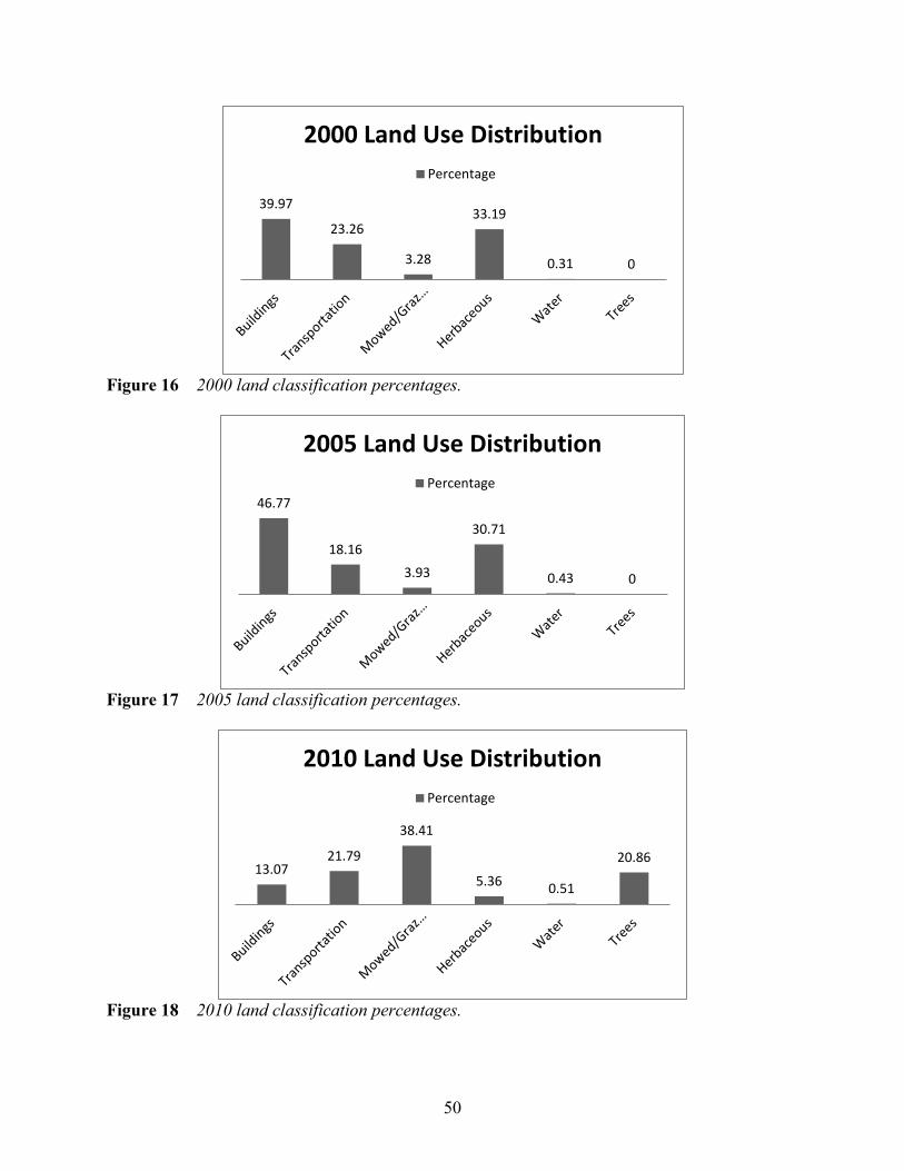
50
Figure 16 2000 land classification percentages.
Figure 17 2005 land classification percentages.
Figure 18 2010 land classification percentages.
39.97
23.26
3.28
33.19
0.31 0
2000 Land Use Distribution Percentage
46.77
18.16 3.93
30.71
0.43 0
2005 Land Use Distribution Percentage
13.07 21.79
38.41
5.36 0.51
20.86
2010 Land Use Distribution Percentage

51
5.2 Storm Water Model Results
Data of soils, showing hydrologic soil groups, and land use classifications were first
joined together to derive the curve numbers for storm water runoff. To estimate the curve
numbers and runoff depth for the study area a curve number look-up table was created and
populated in Microsoft Access. The values were obtained from The Hydraulic Design Manual-
Section 7: NRCS Curve Number Methods – Runoff Curve Number (RCN) which provides
guidance and recommended procedures for the design of Texas department of transportation
drainage facilities (TxDOT, 2011). After the curve number grid was generated the storage
capacity (S) was calculated using the curve numbers. Then the water available for runoff (Q) was
calculated using the storage capacity coefficient in combination with the precipitation input
which was set as five inches for this study. Each process was completed a total of three times,
one for each land survey, indicated previously in this paper.
In Figure 19 the curve number color most dominant is blue, meaning there is a high
propensity for runoff. With 9,761 acres, of the total 12,774 acres, in the category of 91-100 this
represents 76 percent of the total study area. This result is unrealistic considering there is far less
construction and urban development in 2000 than in 2010. This map shows the inaccuracies of
the NCTCOG’s methodology as of 2000 for the land use survey, because the results could not be
used for any type of realistic storm water runoff modeling. The calculations for the runoff depth
(Q), seen in Figure 20, show that nearly the entire study area has a propensity for direct runoff
with no saturation into the ground.
The map representing curve number runoff for 2005, Figure 21, shows the gaps in data
(white spots) that are present. The gaps are a result of the missing transportation infrastructure
that occurred from the beginning despite fixing the majority of the issue when combined with the
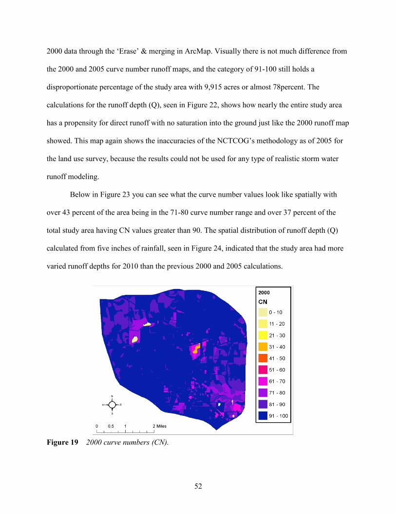
52
2000 data through the ‘Erase’ & merging in ArcMap. Visually there is not much difference from
the 2000 and 2005 curve number runoff maps, and the category of 91-100 still holds a
disproportionate percentage of the study area with 9,915 acres or almost 78percent. The
calculations for the runoff depth (Q), seen in Figure 22, shows how nearly the entire study area
has a propensity for direct runoff with no saturation into the ground just like the 2000 runoff map
showed. This map again shows the inaccuracies of the NCTCOG’s methodology as of 2005 for
the land use survey, because the results could not be used for any type of realistic storm water
runoff modeling.
Below in Figure 23 you can see what the curve number values look like spatially with
over 43 percent of the area being in the 71-80 curve number range and over 37 percent of the
total study area having CN values greater than 90. The spatial distribution of runoff depth (Q)
calculated from five inches of rainfall, seen in Figure 24, indicated that the study area had more
varied runoff depths for 2010 than the previous 2000 and 2005 calculations.
Figure 19 2000 curve numbers (CN).
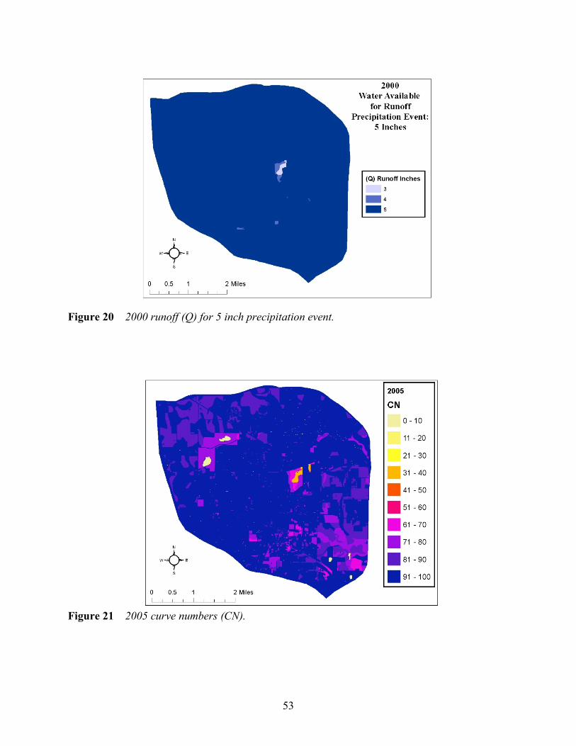
53
Figure 20 2000 runoff (Q) for 5 inch precipitation event.
Figure 21 2005 curve numbers (CN).

54
Figure 22 2005 runoff (Q) for 5 inch precipitation event.
Figure 23 2010 curve numbers (CN).

55
Figure 24 2010 runoff (Q) for 5 inch precipitation event.
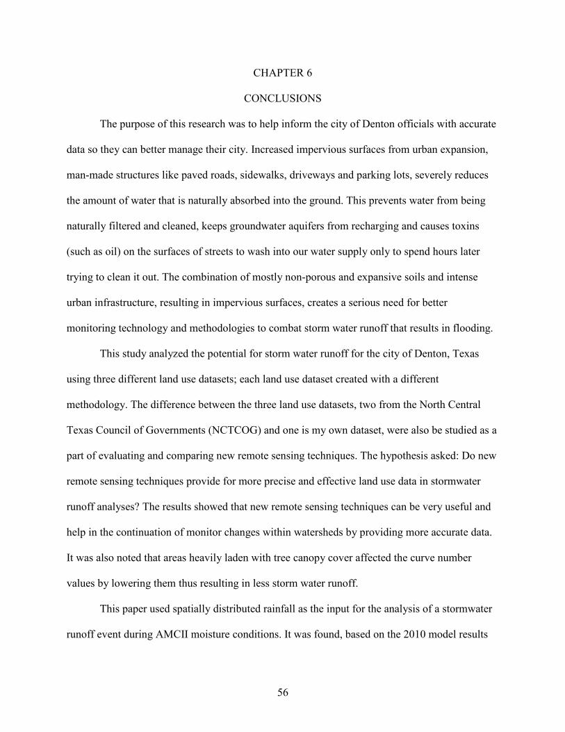
56
CHAPTER 6
CONCLUSIONS
The purpose of this research was to help inform the city of Denton officials with accurate
data so they can better manage their city. Increased impervious surfaces from urban expansion,
man-made structures like paved roads, sidewalks, driveways and parking lots, severely reduces
the amount of water that is naturally absorbed into the ground. This prevents water from being
naturally filtered and cleaned, keeps groundwater aquifers from recharging and causes toxins
(such as oil) on the surfaces of streets to wash into our water supply only to spend hours later
trying to clean it out. The combination of mostly non-porous and expansive soils and intense
urban infrastructure, resulting in impervious surfaces, creates a serious need for better
monitoring technology and methodologies to combat storm water runoff that results in flooding.
This study analyzed the potential for storm water runoff for the city of Denton, Texas
using three different land use datasets; each land use dataset created with a different
methodology. The difference between the three land use datasets, two from the North Central
Texas Council of Governments (NCTCOG) and one is my own dataset, were also be studied as a
part of evaluating and comparing new remote sensing techniques. The hypothesis asked: Do new
remote sensing techniques provide for more precise and effective land use data in stormwater
runoff analyses? The results showed that new remote sensing techniques can be very useful and
help in the continuation of monitor changes within watersheds by providing more accurate data.
It was also noted that areas heavily laden with tree canopy cover affected the curve number
values by lowering them thus resulting in less storm water runoff.
This paper used spatially distributed rainfall as the input for the analysis of a stormwater
runoff event during AMCII moisture conditions. It was found, based on the 2010 model results

57
that the peak runoff increases significantly in the more urbanized areas due to the higher runoff
coefficient. Compared to the available NCTCOG land use survey data, my own 2010 land use
data succeeded at providing for more accurate storm water runoff modeling results. In general,
the NCTCOG is the accepted default-go-to for local free data which many people take advantage
of. The NCTCOG specifically states that the free data they make available should be used for
graphical representation only and the accuracy is not to be taken/used as data produced for
engineering purposes or by a registered professional land surveyor for the state of Texas (North
Central Texas Council of Governments, n.d.). However, individuals with little or no experience
in remote sensing or GIS are more likely to use the free land use data readily available if they
cannot afford to purchase custom high-quality data or make it themselves.
There ended up being some problems encountered throughout the research that should be
highlighted. The land use survey for 2005 from the NCTCOG provided discrepancies in the data
due to a major part of the transportation infrastructure being missing. This could be fixed by
perhaps contacting the NCTCOG directly and discussing with them the purpose behind the
missing information and trying to get better data from them in the future. Also, the land use data
for 2010 could be developed into even more detailed land use categorizations thus generating
even more accurate curve numbers for use in the analysis. As an example, roads could be broken
down into even finer categories based upon their material such as gravel, concrete or asphalt.
6.1 Applications of Data for City
Future approaches to better land management within Denton, Texas should be to instill in
society and researchers the will to create and sustain soil and land conditions that encourage the
infiltration of rainfall where it falls, and to counteract the causes of runoff (Shaxson et al., 2003).
Tree canopy, low bushes, herbs and surface litter provide an excellent protective cover for

58
surface soils from loss of porosity by direct impact of raindrops. Also serving as a food and
energy source for soil organisms, the litter encourages formation of soil organic matter and
faunal passages which ultimately leads to higher infiltration rates (Shaxson et al., 2003). Another
approach the city could take to increase storm water infiltration and slow down runoff is by
detaining the precipitation with physical structures that have been constructed across slopes and
parallel to the surface contour; examples of these include stone lines, walls and earth banks. Also
using large quantities of organic manure, which can be used to fertilize
mowed/grazed/agricultural land, in the place of chemical fertilizers will increase the available
water capacity (AWC) of soils. However the quantities of organic materials required to markedly
increase the AWC are very high so the applications must be continued over many years Shaxson
et al., 2003).
6.2 Future Research
This research could be taken a step farther in the future by adjusting the runoff curve
number (RCN) from the AMCII condition to AMCI and AMCIII conditions. This will give the
city of Denton an even better and more precise idea of how storm water will runoff based on the
pre-existing moisture conditions. AMCI and AMCIII conditions can be calculated from the
existing AMCII value by using the following equations:
CNI = 4.2 x (CNII) 10 - 0.058 x (CNII)
CNIII = 23 x (CNII) 10 + 0.13 x (CNII)
Other suggested future efforts include: (1) The investigation of additional flow events for
the many sub-basins in Denton, TX, (2) study alternative measures of watershed wetness because
the main issues appear to be in assessing an area’s wetness before an event, (3) development of

59
relationships between outlet flow components and water quality parameters, (4) re-evaluating
land-use data to make it even more specific and accurate to the true terrain, (5) compare old
techniques and their accuracy to new ones and also (6) calculate the accumulated flow for each
of the three land use datasets to get an idea of where the water will eventually flow. Something
to also consider for future development is the major benefits of creating a set of standards for
those conducting the research and those relying on the results. As a result there would always be
an agreed upon baseline for all future research and it would help make the flow of information
uniform and concise.

60
REFERENCES Aber, James S., and Susan W. Aber. "Remote Sensing Techniques." Www.geospectra.net.
Emporia State University, 07 Mar. 2002. Web. 24 Apr. 2012. <http://www.geospectra.net/lewis_cl/remote/remote.htm>.
Bisher, Zakaryah Omar Mohamed, Anuar Ahmad, and Maged Mahmoud Marghany. "Accuracy
Assessment of Aerial Triangulation Using Erdas Imagine Software."Academia.edu. Map Asia 2010 & ISG 2010, 26 July 2010. Web. 7 Apr. 2011. <http://teknologimalaysia.academia.edu/AnuarAhmad/Papers/486595/Accuracy_Assessment_of_Aerial_Triangulation_Using_Erdas_Imagine_Software>.
Brown, Karl E. "USGS-NPS Vegetation Mapping Program & Benthic Overview." USGS-NPS Vegetation Mapping Program. Proc. of Benthic Habitat Mapping Workshop, Denver, Colorado. USGS - National Park Service, 03 June 2008. Web. 26 Apr. 2012. <www.nature.nps.govpercent2Fwaterpercent2FUSGSpercent2FPresentationspercent2Fbrown_program_development.ppt&ei=Z8CZT-TLIKqW2AWPjb3-Bg&usg=AFQjCNHYs6B3cJS-cgeAUbX7S-51c7VicA>.
Cambez, M. J., J. Pinho, and L. M. David. "Using SWMM 5 in the Continuous Modeling of
Stormwater Hydraulics and Quality." Proc. of 11th International Conference on Urban Drainage, Edinburgh, Scotland, UK, 2008. N.p., 2008. Web. 06 Apr. 2011. <http://www.hydrolatinamerica.org/jahia/webdav/site/hydrolatinamerica/shared/Reference/Continuouspercent20modellingpercent20percent20withpercent20swmm5_David.pdf>.
City Green. American Forests, 2005. Web. 19 Apr. 2011.
<http://www.americanforests.org/productsandpubs/citygreen/>. Coskun, M., and N. Musaoglu. Investigation of Rainfall-Runoff Modelling of the Van Lake
Catchment by Using Remote Sensing and GIS Integration. Rep. International Society for Photogrammetry and Remote Sensing, 2004. Web. 20 Nov. 2011. <http://www.isprs.org/proceedings/XXXV/congress/comm7/papers/52.pdf>.
Denton-Living.com. The Relocation Professionals, Inc., 2011. Web. 19 Apr. 2011.
<http://www.denton-living.com/weather/>. Ferrell, Aaron C., Ronald B. Scheckenberger, and Raymond T. Guther. "A Case in Support of
Continuous Modeling for Stormwater Management System Design." N.p., 2001. Web. 05 Apr. 2011. <http://www.philipseng.com/papers/Water/Conferencepercent20Final.pdf>.
GeoEye. "GeoEye-1 and IKONOS Feature Comparison." GeoEye Products and Services.
GeoEye, 2011. Web. 30 July 2012. <http://www.geoeye.com/CorpSite/products-and services/imagery-sources/Comparison.aspx>.
Losee, John. Theories of Scientific Progress: An Introduction. New York: Routledge, 2004.
Print.

61
NatureServe. "Accuracy Assessment: Guilford Courthouse National Military Park." Guilford Courthouse National Military Park. U.S. Geological Survey, May 2007. Web. 30 July 2012. <http://biology.usgs.gov/npsveg/guco/aa_rpt.pdf>.
North Central Texas Council of Governments. "2000 Land Use by City." North Central Texas
Council of Governments, 2000. Web. 08 Mar. 2012. <http://www.nctcog.org/ris/demographics/landuse/landuse2000.pdf>.
North Central Texas Council of Governments. "2005 Land Use by City." North Central Texas
Council of Governments, 2005. Web. 08 Mar. 2012. <http://www.nctcog.org/ris/demographics/landuse/landuse2005.pdf>.
North Central Texas Council of Governments. "Frequently Asked Questions." Research &
Information Services. NCTCOG. Web. 08 Mar. 2012. <http://www.nctcog.org/ris/demographics/FAQ.asp>.
North Texas Soil Technical Data. Integrated Foundation Solutions, 2009. Web. 05 May 2011.
<http://www.foundationsolution.com/North_Texas_Soil_Technical_.html>. Ohlhof, Timm. Comparison Study Between ECognition and ERDAS Imagine for the
Classification of High and Moderate Resolution Satellite Imagery. Proc. of 4th ESA-EUSC Conference on Image Information Mining for Security and Intelligence, Madrid-Torrejon. İrfan Akar, 28 Nov. 2006. Web. 07 Apr. 2011. <http://www.irfanakar.com/GIS_Remote_Sensing_files/eCognition%20Definiens/Comparison%20Study%20Between%20eCognition%20and%20ERDAS%20Imagine%20for%20the.pdf>.
Robbins, Clarence, and Stephen P. Phipps. "GIS/Water Resources Tools for Performing
Floodplain Management Modeling Analysis." Proc. of AWRA Symposium on GIS and Water Resources - Sept 22-26, 1996 Ft. Lauderdale, FL. American Water Resources Association, 24 Nov. 1999. Web. 18 Apr. 2011. <http://www.awra.org/proceedings/gis32/woolprt3/>.
Rossman, Lewis. "Storm Water Management Model (SWMM)." EPA. Environmental Protection
Agency, 14 Apr. 2011. Web. 22 Apr. 2011. <http://www.epa.gov/nrmrl/wswrd/wq/models/swmm/>.
Schaefer, Mel, and Bruce Barker. "MGS Flood Continuous Flow Model for Stormwater Facility
Design." Http://www.wsdot.wa.gov. Washington State Department of Transportation, 06 Feb. 2002. Web. 06 Apr. 2011. <http://www.wsdot.wa.gov/publications/fulltext/hydraulics/programs/TrainingSlides.pdf>.
Schiariti, Paul. "Basic Hydrology – Runoff Curve Numbers." Http://njscdea.ncdea.org/. New Jersey Conservation District Employees Association, n.d. Web. 15 Jan. 2012. <http://njscdea.ncdea.org/CurveNumbers.pdf>.

62
Scientific Software Group. "HSSM - Hydrocarbon Spill Screening Models and Modeling/Modelling Software." Scientific Software Group, 2005. Web. 30 July 2012. <http://www.geology-software.com/hssm-model.html>.
Shamsi, Uzair M. GIS Tools for Water, Wastewater, and Stormwater Systems. Reston, VA:
American Society of Civil Engineers, 2002. Print. Shaxson, T. F., and Richard G. Barber. Optimizing Soil Moisture for Plant Production: The
Significance of Soil Porosity. Rome: Food and Agriculture Organization of the United Nations, 2003. Food and Agriculture Organization of the United Nations, 2003. Web. 24 Apr. 2012. <http://www.fao.org/docrep/006/y4690e/y4690e00.htm#Contents>.
Soil Datasets. Penn State University, 06 May 1998. Web. 18 Apr. 2011.
<http://www.soilinfo.psu.edu/index.cgi?soil_data>. Stats about All US Cities. Advameg, Inc., 2011. Web. 24 Apr. 2012.
<http://www.city-data.com/>. Success Stories. American Forests. Web. 20 Apr. 2011.
<http://www.americanforests.org/productsandpubs/citygreen/success.php>. Swiecki, T. J., and E. A. Bernhardt. Guidelines for Developing and Evaluating Tree Ordinances.
Phytosphere Research, 31 Oct. 2001. Web. 06 Apr. 2011. <http://phytosphere.com/treeord/index.htm>.
Tan, C. H., S. F. Shih, A. M. Melesse, J. D. Jordan, and S. S. Yeh. Remote Sensing and
Geographic Information System in Runoff Coefficient Estimation for Irrigated Regions. Proc. of International Commission on Irrigation and Drainage - 1st Asian Regional Conference Seoul, 2001. Chinese Taipei Committee, International Commission on Irrigation and Drainage, 2001. Web. 10 Jan. 2012. <http://ctcid.water.tku.edu.tw/admin/upload/paper/2001-Tan.C.H.pdf>.
"The Hydrocarbon Spill Screening Model (HSSM), US EPA | Ecosystems Research Division US
EPA." US Environmental Protection Agency. 19 Jan. 2011. Web. 05 Apr. 2011. <http://www.epa.gov/athens/hssm1.html>.
TxDOT. "Hydraulic Design Manual." Search. TxDOT, Oct. 2011. Web. 13 Feb. 2012.
<http://onlinemanuals.txdot.gov/txdotmanuals/hyd/manual_notice.htm>. United States of America. U.S. Environmental Protection Agency. Athens, Georgia 30613.Storm
Water Management Model, Version 4: User's Manual. By Wayne C. Huber and Robert E. Dickinson. N.p., Oct. 1992. Web. 05 Apr. 2011. <http://sdi.odu.edu/mbin/swmm/swmm_1.pdf>.

63
University of Arkansas. "Impervious Surface Mapping with High Resolution Satellite Imagery."Earth Case Study. Definiens Ecognition, 2003. Web. 07 Apr. 2011. <http://www.ecognition.com/sites/default/files/defienens_arkansas.high_resolution_satellite_imagery.pdf>.
Van Mullem, Joseph A., Donald E. Woodward, Richard H. Hawkins, and Allen T. Hjelmfelt Jr.
"RUNOFF CURVE NUMBER METHOD: BEYOND THE HANDBOOK”, 24 May 2004. Web. 20 Apr. 2011. < http://www.mmnt.net/db/0/0/ftp-fc.sc.egov.usda.gov/NWMC/CN_info >.
Viera, Deborah. Environmentally Sensitive Areas & Watershed Protection Plans., 25 Oct. 2010.
Web. 22 Feb. 2011. <http://riparianworkshop.org/downloads/environmentally-sensitive.pdf>.
"Watershed." Watershed. City of Denton, TX, 2011. Web. 24 Apr. 2012.
<http://www.cityofdenton.com/index.aspx?page=181>. Weaver, James W. "Application of the Hydrocarbon Spill Screening Model to Field Sites."
American Society of Civil Engineers, 14 Nov. 1996. Web. 5 Apr. 2011. <http://www.epa.gov/nerl/mtbe/application_hydrocarbon.pdf>.
Wilson, A. G. Geography and the Environment: Systems Analytical Methods. Chichester: J.
Wiley, 1981. Print. Yang, Ming-Der, Carolyn J. Merry, and Robert M. Sykes. "AWRA GIS Symposium –
Adaptive Short-Term Water Quality Forecasts Using Remote Sensing and GIS." American Water Resources Association (AWRA). AWRA SYMPOSIUM ON GIS AND WATER RESOURCES, 22 Sept. 1996. Web. 07 Apr. 2011. <http://www.awra.org/proceedings/gis32/yang/>.
Zoppou, Christopher. Review of Storm Water Models. Tech. no. 52/99. CSIRO Land and
Water, Dec. 1999. Web. 22 Mar. 2011. <http://www.clw.csiro.au/publications/technical99/tr52-99.pdf>.
Top Related