


Languages
Pages
Legal


ECMWF workshop on Ocean-Atmosphere Interactions, 10-12 Nov 2008
A revised ocean-atmosphere physical coupling interface
and about technical coupling software
S. Valcke (CERFACS) E. Guilyardi (IPSL/LOCEAN & CGAM)
with numerous contributions from the community

ECMWF workshop on Ocean-Atmosphere Interactions, 10-12 Nov 2008
Outline
Part I –
On an revised ocean-atmosphere physical coupling interface• Context and guidelines for the design of a new physical interface• The physical exchanges• Time sequence of exchanges
Part II -
About technical coupling software• Different technical solutions to assemble model codes•The OASIS coupler (historic, community, …)• Regridding
algorithms in OASIS
• 1st order conservative remapping (2nd
order, SUBGRID)
• Non-matching sea-land mask• Vector interpolation
ECMWF workshop on Ocean-Atmosphere Interactions, 10-12 Nov 2008
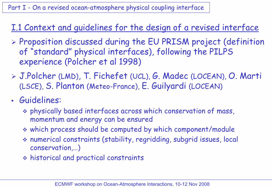
I.1 Context and guidelines for the design of a revised interfaceProposition discussed during the EU PRISM project (definition of “standard” physical interfaces), following the PILPS experience (Polcher et al 1998)J.Polcher (LMD), T. Fichefet (UCL), G. Madec (LOCEAN), O. Marti (LSCE), S. Planton (Meteo-France), E. Guilyardi (LOCEAN)
• Guidelines:physically based interfaces across which conservation of mass, momentum and energy can be ensuredwhich process should be computed by which component/modulenumerical constraints (stability, regridding, subgrid issues, local conservation,…)historical and practical constraints
Part I -
On a revised ocean-atmosphere physical coupling interface

1*- Sensible heat flux
6*- Evaporation + int. energy [+ Qlat ]
ECMWF workshop on Ocean-Atmosphere Interactions, 10-12 Nov 2008
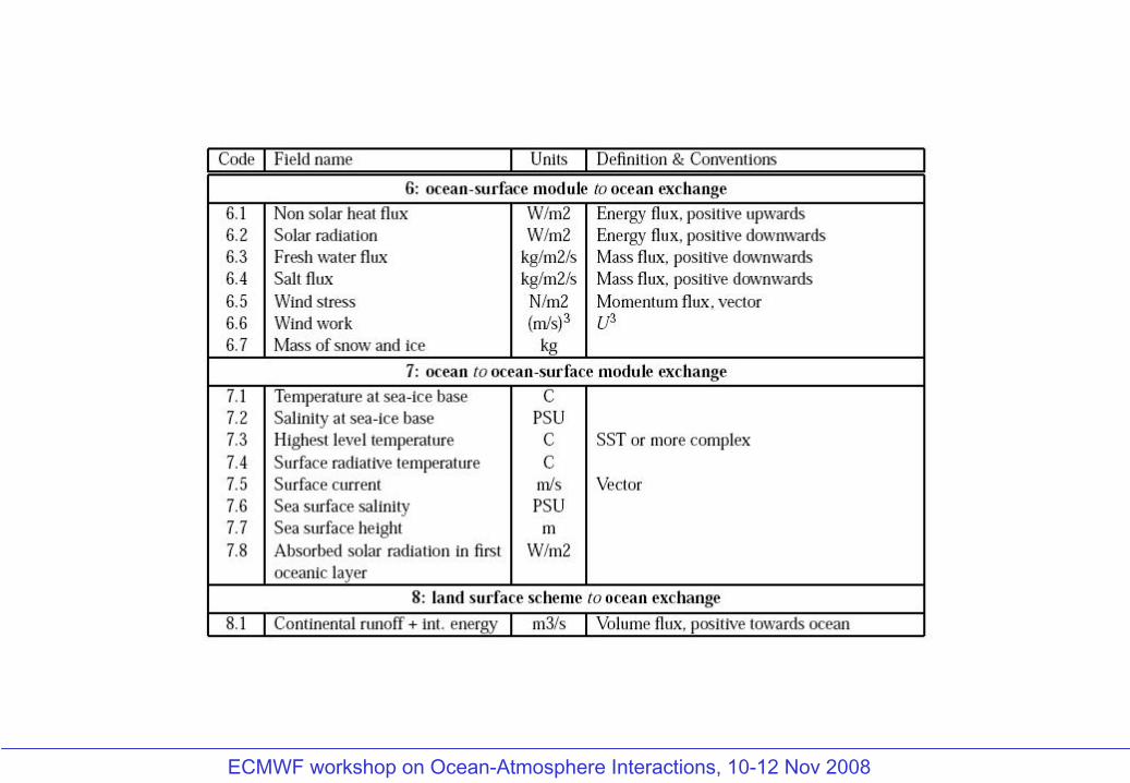
3x- Fresh water flux4x- Salt flux7x- Mass of snow and ice
1- Temperature at sea-ice base3- Highest level temperature (SST)4- Ocean radiative temp.8- Absorbed solar radiation (in 1st layer)5- Surface ocean current7- Surface height 7
1- Continental runoff+ internal Energy 8
1*- Surf. Temp2*- Surf. Roughness3*- Displacement height4x- Surface velocity
5
1- Rainfall + int. energy2- Snowfall + int. energy
3- Incoming solar radiat.4- Solar zenith angle5- Fraction of diffuse
solar radiation6- Downward infrared
radiation7- Sensitivity of atmos
temp. & humidity tosurf. fluxes
1 1
2*- Surf. emissivity 3*- Albedo, direct4*- Albedo, diffuse5*- Surf. radiative temp.
2
2
Land surface model
Ocean model
Atmosphere model
Ocean surface module
Sea ice model (wave model)
Surface layer turbulence
Part I -
On a revised ocean-atmosphere physical coupling interfaceI.2 The physical exchanges
6
1x- Non solar heat flux2x- Solar radiation
7*- Wind stress
5x- Wind stress6x- U^3
8- Subgrid fractions
Note on subgrid fractiondependance:<>x- Sea Ice categories
(incl. open ocean)<>*- Sea Ice or Land Surf.
categories8- Subgrid fractions2- Salinity at sea-ice base6- Sea surface salinity
1*- ρCd 42*- ρCe 43*- ρCh
1- Surface pressure2-4 Air temperature, humidity and wind5- Mean scalar wind speed6- Height of these variables 3
3

ECMWF workshop on Ocean-Atmosphere Interactions, 10-12 Nov 2008
I.3 Time sequence of exchanges
Atm
SLT
OSM
Oce
7
5
6sea ice
t
Frequency of coupling exchanges:
F7 = F6 < F5 = F3 = F1 = F4 = F2
slow fast
3
1
4+3
Comp.Fluxes
2
atm
t (implicit)
3
1
4+3
25
3
1
4+3
2
3
1
4+3
2
7
deep ocean
t
Part I -
On a revised ocean-atmosphere physical coupling interface
5 5
6

ECMWF workshop on Ocean-Atmosphere Interactions, 10-12 Nov 2008
Separation of fast ocean + sea ice surface processes involving heat, water and momentum exchanges with the atmosphere from slower deeper ocean processes.
Calculation of fluxes at the resolution of the surface (would be non-physical to regrid the turbulent exchange coefficients Cd, Ce, Ch).
Implicit calculation of energy fluxes from the base of the sea-ice to the top of the atmosphere.
Part I -
On a revised ocean-atmosphere physical coupling interface
Comments and conclusions• Increased modularity with SLT and OS modules.
• SLT runs on finer grid and computes surface turbulent coefficient.
• OS computes radiation and turbulent fluxes.
ECMWF workshop on Ocean-Atmosphere Interactions, 10-12 Nov 2008
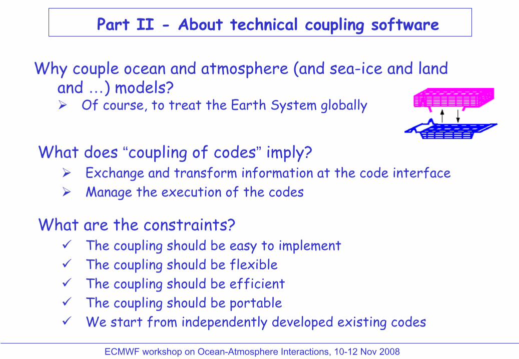
Why couple ocean and atmosphere (and sea-ice and land and …) models?
Of course, to treat the Earth System globally
Part II -
About technical coupling software
What does “coupling of codes” imply?Exchange and transform information at the code interfaceManage the execution of the codes
What are the constraints?The coupling should be easy to implementThe coupling should be flexibleThe coupling should be efficientThe coupling should be portableWe start from independently developed existing codes

ECMWF workshop on Ocean-Atmosphere Interactions, 10-12 Nov 2008
II.1 Different technical solutions to assemble model codes:
Part II -
About technical coupling software
2.
use existing communication protocole
(MPI, CORBA, UNIX pipe, files, …)
program prog2…call xxx_recv (prog1, data)end
program prog1…call xxx_send (prog2, data, …)end
easyflexible
☺
efficient☺
portableexisting codes
easyflexible(efficient)(portable)
☺
existing codes
program prog1…call sub_prog2(data)…end prog1
1.
merge the codes:program prog2subroutine sub_prog2(data)…end prog2
ECMWF workshop on Ocean-Atmosphere Interactions, 10-12 Nov 2008
(easy)☺
flexible
☺
efficient☺
portable(existing codes)
prog1_u1 prog2_u1
coupling
prog1_u2 prog1_u3
couplingprog2_u2
Adapt code data structures
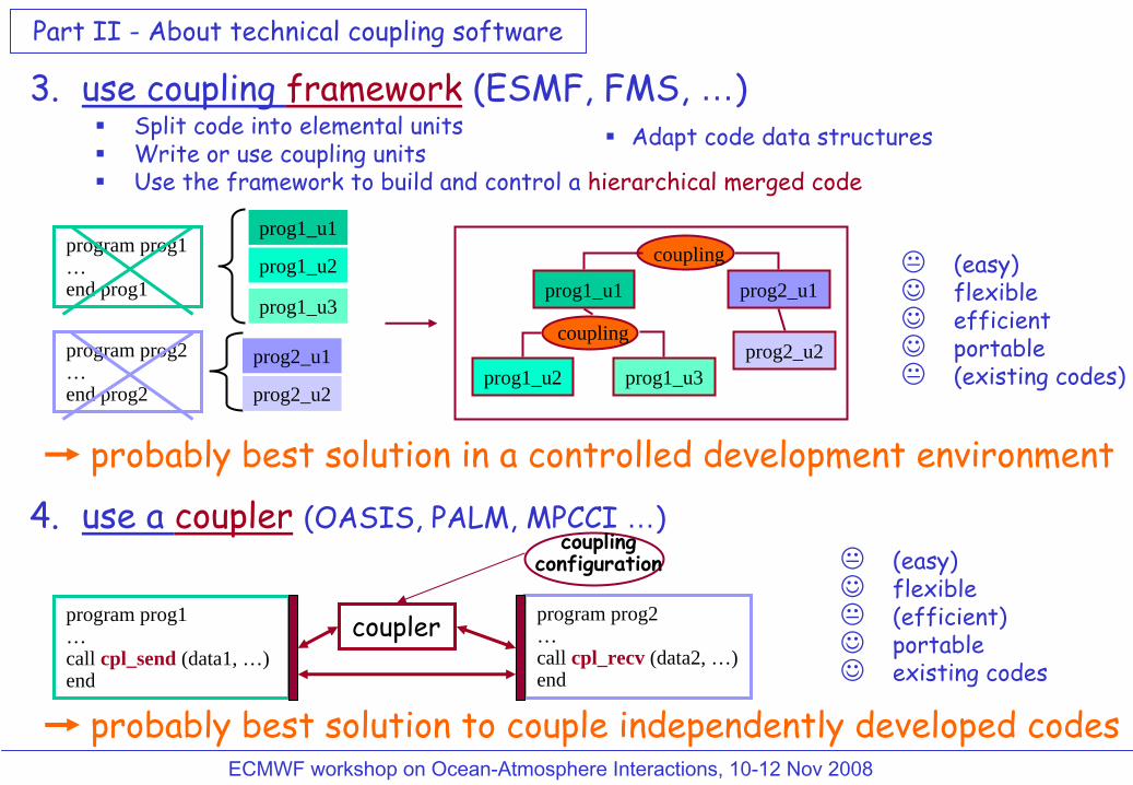
3.
use coupling framework
(ESMF, FMS, …)Split code into elemental unitsWrite or use coupling unitsUse the framework to build and control a hierarchical merged code
program prog1…end prog1
prog1_u1
prog1_u2
prog1_u3
program prog2…end prog2
prog2_u1
prog2_u2
(easy)☺
flexible(efficient)
☺
portable☺
existing codes
probably best solution in a controlled development environment4.
use a coupler
(OASIS, PALM, MPCCI …)
program prog2…call cpl_recv (data2, …)end
program prog1…call cpl_send (data1, …)end
coupler
couplingconfiguration
Part II -
About technical coupling software
probably best solution to couple independently developed codes

ECMWF workshop on Ocean-Atmosphere Interactions, 10-12 Nov 2008
1991
2001|-- |--- PRISM OASIS 1 OASIS 2 OASIS3
OASIS4 OASIS1, OASIS2, OASIS3:•low resolution, low number of 2D fields, low coupling frequency:
flexibility very important, efficiency not so much!New OASIS3_3 release in the next few weeks!
OASIS4:•high resolution parallel models, massively parallel
platforms, 3D fields
need to optimise and parallelise the couplerOASIS4 beta version available
II.2 The OASIS coupler
developed by CERFACS since 1991 to couple existing GCMscurrently an active collaboration between NLE-IT, CNRS and CERFACS
Part II -
About technical coupling software

ECMWF workshop on Ocean-Atmosphere Interactions, 10-12 Nov 2008
II.2.1 OASIS community today•CERFACS (France) ARPEGE3-ORCA2/LIM, ARPEGE4-NEMO/LIM-TRIP•METEO-FRANCE (France) ARPEGE4-ORCA2, ARPEGE3-OPAmed ARPEGE3-OPA8.1/GELATO•IPSL-
LODYC, LMD, LSCE (France) LMDz-ORCA2/LIM LMDz-ORCA4 ORCA4•MPI-M&D (Germany) ECHAM5-MPI-OM, ECHAM5-C-HOPE, PUMA-C-HOPE, EMAD-E-HOPE•ECMWF IFS -
CTM (GEMS), IFS -
ORCA2 (MERSEA)•MET Office (UK)
MetOffice
ATM -
NEMO•IFM-GEOMAR (Germany)
ECHAM5 -
NEMO (OPA9-LIM) •NCAS / U. Reading (UK)
ECHAM4 -
ORCA2 HADAM3-ORCA2•SMHI (Sweden) RCA(region.) –
RCO(region.)•NERSC (Norway)
ARPEGE -
MICOM, CAM -
MICOM•KNMI (Netherlands)
ECHAM5 -
TM5/MPI-OM•INGV (Italy)
ECHAM5 –
MPI-OM•ENEA (Italy) MITgcm
-
REGgcm•JAMSTEC (Japan)
ECHAM5(T106) -
ORCA ½
deg•IAP-CAS (China) AGCM -
LSM•KMA (Korea)
CAM3 –
MOM4•BMRC (Australia) BAM3–MOM2, BAM5–MOM2, TCLAPS-MOM•CSIRO (Australia)
Sea Ice code -
MOM4•RPN-Environment Canada (Canada)
MEC -
GOM•UQAM (Canada)
GEM -
RCO•U. Mississippi (USA)
MM5 -
HYCOM•IRI (USA)
ECHAM5 -
MOM3•JPL (USA)
UCLA-QTCM -
Trident-Ind4-Atlantic
Part II -
About technical coupling software

ECMWF workshop on Ocean-Atmosphere Interactions, 10-12 Nov 2008
II.3 Regridding
algorithms available in OASIS(Los Alamos SCRIP library, Jones 1999)
• bilinear interpolationgeneral bilinear iteration in a
continuous local coordinate systemusing f(x) at x1
, x2
, x3
, x4
x11 x22
x33 x44
xx x xxxx
xxx
xxx
xxx
general bicubic iteration continuous local coordinate system: f(x), δf(x)/δi, δf(x)/δj, δ2f/δiδj in x1, x2, x3, x4for logically-rectangular grids (i,j)
x11 x22
x33 x44
standard bicubic algorithm: 16 neighbour points
for Gaussian Reduced grids
• bicubic
interpolation: conserves 2nd
order properties such as wind curl
• n-nearest-neighbours: weight(x) α
1/dd: great circle distance on the sphere:d = arccos[sin(lat1)*sin(lat2) + cos(lat1)*cos(lat2) * cos(lon1-lon2)]
• gaussian weighted n-neighbours: weigth(x) α
exp(-1/2
d2/σ2)
x: source grid pointtarget grid point
d
xx
Part II -
About technical coupling software
ECMWF workshop on Ocean-Atmosphere Interactions, 10-12 Nov 2008
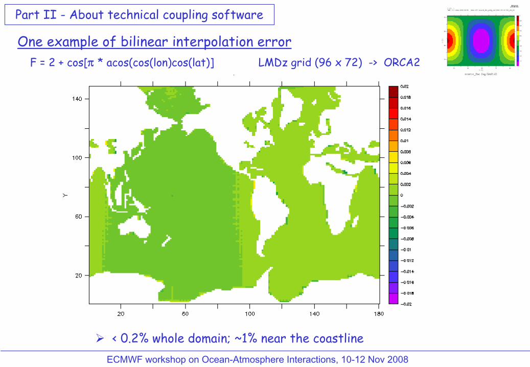
One example of bilinear interpolation errorF = 2 + cos[π
* acos(cos(lon)cos(lat)] LMDz
grid (96 x 72) -> ORCA2
< 0.2% whole domain; ~1% near the coastline
Part II -
About technical coupling software
ECMWF workshop on Ocean-Atmosphere Interactions, 10-12 Nov 2008
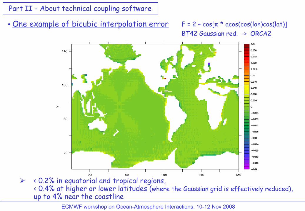
• One example of bicubic
interpolation error F = 2 –
cos[π
* acos(cos(lon)cos(lat)]BT42 Gaussian red. -> ORCA2
< 0.2% in equatorial and tropical regions,< 0.4% at higher or lower latitudes (where the Gaussian grid is effectively reduced), up to 4% near the coastline
Part II -
About technical coupling software
ECMWF workshop on Ocean-Atmosphere Interactions, 10-12 Nov 2008
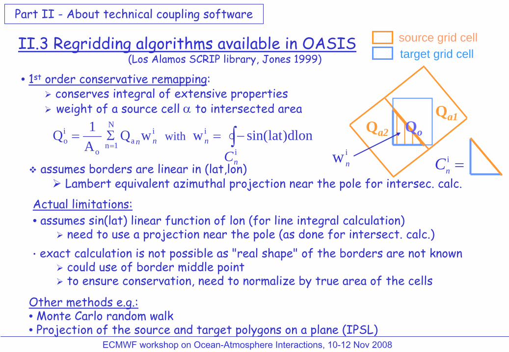
II.3 Regridding
algorithms available in OASIS (Los Alamos SCRIP library, Jones 1999)
assumes borders are linear in (lat,lon)Lambert equivalent azimuthal projection near the pole for intersec. calc.
source grid celltarget grid cell
• 1st
order conservative remapping: conserves integral of extensive propertiesweight of a source cell α to intersected area
∫ −=Σ==
i
iia
N
1no
io dlon)latsin( w wQ
A1 Q with
n
nnn
C
Qa1Qa2 Qo
i w n =i nC
Other methods e.g.:• Monte Carlo random walk• Projection of the source and target polygons on a plane (IPSL)
Part II -
About technical coupling software
Actual limitations:• assumes sin(lat) linear function of lon
(for line integral calculation)
need to use a projection near the pole (as done for intersect. calc.)• exact calculation is not possible as "real shape" of the borders are not known
could use of border middle pointto ensure conservation, need to normalize by true area of the cells

ECMWF workshop on Ocean-Atmosphere Interactions, 10-12 Nov 2008
• One example of conservative remapping error F = 2 –
cos[π
* acos(cos(lon)cos(lat)]ORCA2 -> LMDz
(96x72)
< 0.2% everywhere except~ 0.8% for LMDz
last row close to the North pole
~ 2% near the coastline
Part II -
About technical coupling software

ECMWF workshop on Ocean-Atmosphere Interactions, 10-12 Nov 2008
II.4 Problem with 1st
order conservative remapping
(low to high resolution) :
• Solution 1: use 2nd
order conservative remapping:
wQ)(cos
1 wQ wQ Q i3
ai2
ai1a
io lonlatlat ∂
∂+
∂∂
+=
aa T, Q
io
io T , Q
Part II-
About technical coupling software
Solar type:
• Solution 2: use SUBGRID transformation:
Non-solar type:
aa
ioi
o Q)– (1)– (1 Q
αα
=
)TT(TQQ Q a
io
TT
aa
io
a
−∂∂
+== *conservative if αa
/Ta
correspond to conservative remapping of αo
/Toi i

ECMWF workshop on Ocean-Atmosphere Interactions, 10-12 Nov 2008
II.5 Problem with non-matching sea-land masks wQ A1 Q i
a
N
1no
io nn=
Σ=
1-
Ideally: Support subsurfaces
in the atmosphere and use the ocean land-sea mask in the atmosphere to determine the fractional area of each type of surface
2-“DESTAREA”
optionlocal flux conservationpossibly unrealistic flux values
=oA W
3-“FRACAREA”
optionno local conservation of fluxrealistic flux values
+ nearest non-masked value for ocean cells covered only with masked atmospheric cells
=oA W
L W
W
L W
W
no local conservation of flux
global conservation can be artificially imposed
Part II -
About technical coupling software
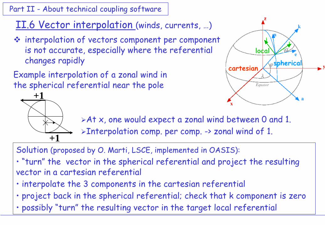
II.6 Vector interpolation (winds, currents, …)
local
sphericalcartesian
interpolation of vectors component per component is not accurate, especially where the referential changes rapidly
Example interpolation of a zonal
wind in the spherical referential near the pole
+1
+1
At x, one would expect a zonal wind between 0 and 1.Interpolation comp. per comp. -> zonal wind of 1.
Solution (proposed by O. Marti, LSCE, implemented in OASIS):•
“turn”
the vector in the spherical referential and project the resulting
vector in a cartesian
referential• interpolate the 3 components in the cartesian
referential
• project back in the spherical referential; check that k component is zero• possibly “turn”
the resulting vector in the target local referential
Part II -
About technical coupling software

ECMWF workshop on Ocean-Atmosphere Interactions, 10-12 Nov 2008
Conclusions• Different technical solutions to assemble model codes:
•Coupling framework (e.g. ESMF): best solution in a controlled development environment
•Coupler (e.g. OASIS): best solution to couple independently developed codes
• The OASIS coupler :• Coarse to fine grid remapping: subgrid
variability with 2nd
order
remapping or SUBGRID (1st
order Taylor expansion)
• Non-matching sea-land masks: • DESTAREA: local flux conservation but unrealistic flux values• FRACAREA: no local flux conservation but realistic flux values• Global conservation can be artificially imposed
• Vector interpolation: need to project components in a cartesian referential before interpolation.
Part II -
About technical coupling software

ECMWF workshop on Ocean-Atmosphere Interactions, 10-12 Nov 2008
The end
ECMWF workshop on Ocean-Atmosphere Interactions, 10-12 Nov 2008
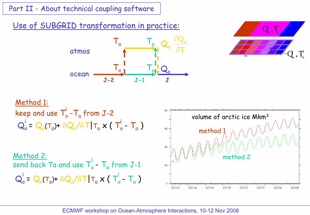
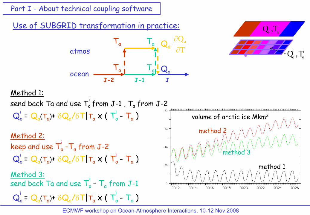
Use of SUBGRID transformation in practice:aa T, Q
io
io T , Q
method 1
method 2
To
QaTa
QoJ-2 J-1 J
ocean
atmos
To
TaT
Qa
∂∂
Part II -
About technical coupling software
volume of arctic ice Mkm3
Method 1: keep and use To
-Ta
from J-2Qo
=
Qa(Ta)+
δQa
/δT|Ta
x ( To
-
Ta
)i i
i
Method 2: send back Ta and use To
-
Ta
from J-1
Qo
=
Qa(Ta)+
δQa
/δT|Ta
x ( To
-
Ta
)i i
i

ECMWF workshop on Ocean-Atmosphere Interactions, 10-12 Nov 2008
ECMWF workshop on Ocean-Atmosphere Interactions, 10-12 Nov 2008
Part II -
About technical coupling software
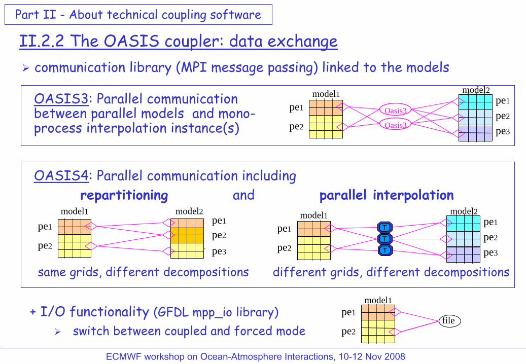
communication library (MPI message passing) linked to the models
II.2.2 The OASIS coupler: data exchange
+ I/O functionality (GFDL mpp_io
library)switch between coupled and forced mode
pe1
pe2
model1
file
ECMWF workshop on Ocean-Atmosphere Interactions, 10-12 Nov 2008
OASIS4: Parallel communication includingrepartitioning
and parallel interpolation
pe1
pe2
model1pe1
pe2
pe3
pe1
pe2
model1 pe1
pe2
pe3
model2
TTT
model2
same grids, different decompositions different grids, different decompositions
Oasis3
pe1
pe2
model1
Oasis3pe1
pe2
pe3
model2OASIS3: Parallel communication between parallel models and mono-
process interpolation instance(s)
ECMWF workshop on Ocean-Atmosphere Interactions, 10-12 Nov 2008
Use of SUBGRID transformation in practice:aa T, Q
io
io T , Q
method 2
method 3
To
QaTa
QoJ-2 J-1 J
ocean
atmos
To
TaT
Qa
∂∂
method 1
Part I -
About technical coupling software
volume of arctic ice Mkm3
Method 2: keep and use To
-Ta
from J-2Qo
=
Qa(Ta)+
δQa
/δT|Ta
x ( To
-
Ta
)i i
i
Method 1: send back Ta and use To from J-1 , Ta
from J-2Qo
=
Qa(Ta)+
δQa
/δT|Ta
x ( To
-
Ta
)i i
i
Method 3: send back Ta and use To
-
Ta
from J-1
Qo
=
Qa(Ta)+
δQa
/δT|Ta
x ( To
-
Ta
)i i
i

ECMWF workshop on Ocean-Atmosphere Interactions, 10-12 Nov 2008
Remapping algorithms available in OASIS (Los Alamos SCRIP library)
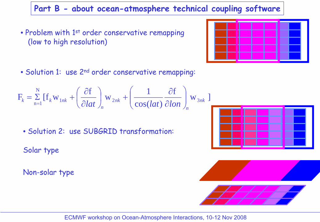
Part B -
about ocean-atmosphere technical coupling software
Actual limitations:• borders are linear in (lat,lon) between corners (for intersection calculation)
uses Lambert equivalent azimuthalprojection near the pole
• sin(lat) linear function of in lon
(for line integral calculation); fractional error is < .001 further than 10 deg from the pole, and only ~0.1 within about 1 deg of it, for the ORCA1 example (for most gridcells
the two measures of gridcell
area
agree to < 5%, but for two gridcells
they're out by 10%, and for another two they're out by 50%.
need to use a projection for line integral calculation too
•
exact calculation is not possible as "real shape" of the borders are not known
to ensure conservation, need to normalize by true area of the cells (i.e. as considered by the models themselves)
ECMWF workshop on Ocean-Atmosphere Interactions, 10-12 Nov 2008
Part B -
about ocean-atmosphere technical coupling software
• Problem with 1st
order conservative remapping(low to high resolution)
• Solution 1: use 2nd
order conservative remapping:
] wf)(cos
1 wf w[f F 321
N
1n nkn
nkn
nkkk lonlatlat ⎟⎟⎠
⎞⎜⎜⎝
⎛∂∂
+⎟⎠⎞
⎜⎝⎛∂∂
+Σ==
• Solution 2: use SUBGRID transformation:
Solar type
Non-solar type
ECMWF workshop on Ocean-Atmosphere Interactions, 10-12 Nov 2008
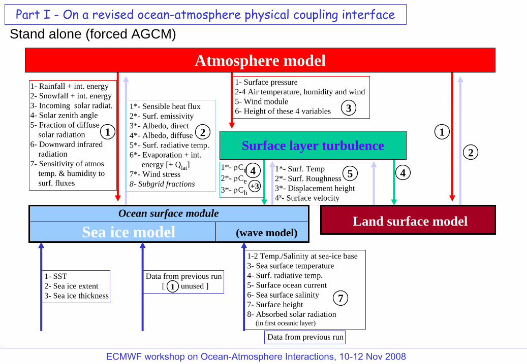
1- Rainfall + int. energy2- Snowfall + int. energy3- Incoming solar radiat.4- Solar zenith angle5- Fraction of diffuse
solar radiation6- Downward infrared
radiation7- Sensitivity of atmos
temp. & humidity tosurf. fluxes
1*- Sensible heat flux2*- Surf. emissivity 3*- Albedo, direct4*- Albedo, diffuse5*- Surf. radiative temp.6*- Evaporation + int.
energy [+ Qlat ]7*- Wind stress8- Subgrid fractions
1- Surface pressure2-4 Air temperature, humidity and wind5- Wind module6- Height of these 4 variables
1*- ρCd2*- ρCe3*- ρCh
1*- Surf. Temp2*- Surf. Roughness3*- Displacement height4x- Surface velocity
1 2
3
4 5
Ocean surface module
Surface layer turbulence
Sea ice model (wave model)
+34
1
2
Atmosphere model
Land surface model
1- SST2- Sea ice extent3- Sea ice thickness
Data from previous run[ unused ]1
1-2 Temp./Salinity at sea-ice base3- Sea surface temperature4- Surf. radiative temp.5- Surface ocean current6- Sea surface salinity7- Surface height8- Absorbed solar radiation
(in first oceanic layer)
7
Data from previous run
Stand alone (forced AGCM)Part I -
On a revised ocean-atmosphere physical coupling interface
Top Related