


Languages
Pages
Legal


A precise method for visualizing dispersive features in image plots
Peng Zhang, P. Richard, T. Qian, Y. -M. Xu, X. Dai, and H. Ding
• Institute of Physics, Chinese Academy of Sciences • Advanced Light Source, Lawrence Berkeley National
Laboratory

Introduction • Second derivative is widely used to get a better
visualization of the band dispersions in ARPES intensity plot.

Second derivative in Digital Image Processing
• Moon picture from NASA processed by the Laplacian filter.
Digital Image Processing, Rafael C. Gonzalez, Richard E. Woods, Prentice Hall (2001)

Why second derivative?
• There is no theory claiming that second derivatives will recover the peak features.
Parabola and its second derivative

Curvature and curve peaks
Curvature is a measure of the amount of curving. 2
32 ))(1(
)()(xf
xfxC′+
′′=
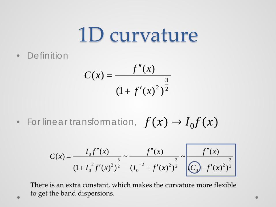
1D curvature • Definition
• For linear transformation, 𝑓(𝑥) → 𝐼0𝑓(𝑥)
23
2 ))(1(
)()(xf
xfxC′+
′′=
23
20
23
220
23
220
0
))((
)(~))((
)(~))(1(
)()(xfC
xf
xfI
xf
xfI
xfIxC′+
′′
′+
′′
′+
′′=
−
There is an extra constant, which makes the curvature more flexible to get the band dispersions.

The arbitrary constant • When C0 goes to infinity
Curvature is the same as second derivative. • When C0 goes to 0
Curvature peaks approach the original peaks.
f‘(x) is 0 at peak positions

A computting tip
• f‘(x) can be in a very wide range depending on data. To make the constant more robust, it is better to normalize f’(x) by its maximum.
• The reasonable range of a0 is about 10 ~ 0.001. (However, you can go further, depending on the data.)
23
2max
20
23
20 )|)(|/)((
)(~))((
)(~)(xfxfa
xf
xfC
xfxC′′+
′′
′+
′′

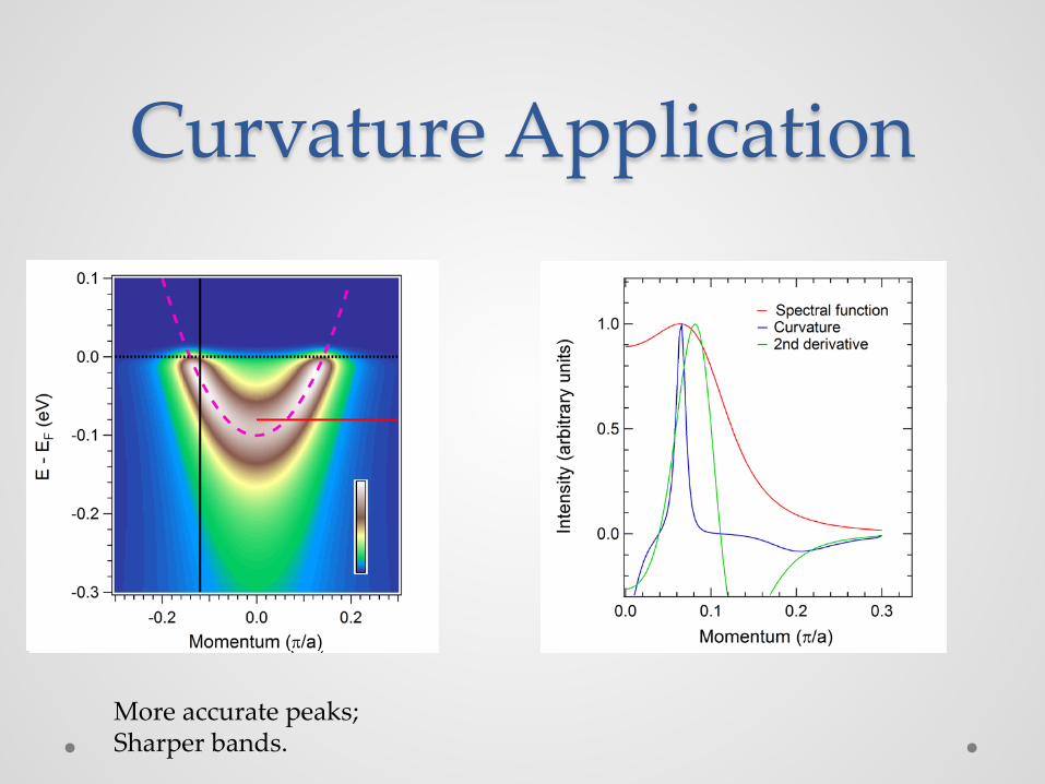
Curvature Application
More accurate peaks; Sharper bands.
Curvature Application
More accurate peaks; Sharper bands.

Curvature Application
Second derivative
Curvature More accurate peaks; Sharper bands.

Curvature Application
Advantages: • More
accurate peaks;
• Sharper bands.
Phys. Rev. Lett. 102, 047003 (2009)
Physical Review B 83, 140513(R) (2011)
Raw data Second derivative Curvature
Ba0.6K0.4Fe2As2
Sr4V2O6Fe2As2

2D Lapalace Operator • In ARPES data, we cannot use Laplacian filter since the
dimensions of the two terms are different.
• We can start from the Taylor expansion
• Using the second order terms
• We got
∇2 f =∂ 2 f∂x 2 +
∂ 2 f∂y 2
∆f =∂ 2 f∂x 2 (∆x)2 +
∂ 2 f∂y 2 (∆y)2
∆f ~ ∆f(∆y)2 =
∂ 2 f∂x 2 (∆x
∆y)2 +
∂ 2 f∂y 2
2 2 2 22 20 0 0 0 0 0 0 0 0 0
0 0 0 0 2 2 2
( , ) ( , ) ( , ) ( , ) ( , )( , ) ( , ) ( ) ( ( ) ( ) 2 ( )) ...f x y f x y f x y f x y f x yf x x y y f x y x y x y x yx y x y x y
∂ ∂ ∂ ∂ ∂∂ ∂ ∂ ∂ ∂ ∂
+ ∆ + ∆ = + ∆ + ∆ + ∆ + ∆ + ∆ ∆ +

Application
Horizontal second derivative
Vertical second derivative
2D second derivative
Raw data

2D curvature • Mean curvature in 2D
• Making replacements:
Where Cx=(I0∆x)2, Cy=(I0∆y)2
2 2 22 2
2 2
32 2 2
[1 ( ) ] 2 [1 ( ) ]( , )
[1 ( ) ( ) ]
f f f f f f fx y x y x y y xC x y
f fx y
∂ ∂ ∂ ∂ ∂ ∂ ∂∂ ∂ ∂ ∂ ∂ ∂ ∂ ∂
∂ ∂∂ ∂
+ − + +=
+ +
𝜕𝑓𝜕𝑥
→ 𝜕𝑓𝜕𝑥𝐼0∆𝑥 , 𝜕𝑓
𝜕𝑦 → 𝜕𝑓
𝜕𝑦𝐼0∆𝑦

2D Curvature Application
• 2D curvature method gives a much better representation of the original character, with very sharp strokes.
• Only little distortion can be observed near stroke intersections and near the beginning and the end of each stroke.
2D second derivative Raw data 2D curvature
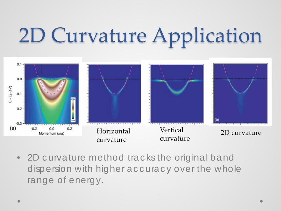
2D Curvature Application
• 2D curvature method tracks the original band dispersion with higher accuracy over the whole range of energy.
Horizontal curvature
Vertical curvature
2D curvature

2D Curvature Application • Fermi surface contour of Ba0.6K0.4Fe2As2
Raw data 2D second derivative 2D curvature

Igor Macro online
Top Related