TEL AVIV UNIVERSITYTHE IBY AND ALADAR FLEISCHMAN FACULTY OF ENGINEERING

A Note on Distributed Stable Matching

Thesis submitted towards the degree of

“Master of Science in Electrical Engineering”

by

Alex Kipnis

November, 2008

TEL AVIV UNIVERSITYTHE IBY AND ALADAR FLEISCHMAN FACULTY OF ENGINEERING

A Note on Distributed Stable Matching

Thesis submitted towards the degree of

“Master of Science in Electrical Engineering”

by

Alex Kipnis

This research was carried out in the

Department of Electrical Engineering - Systems,

Tel-Aviv University

Under the supervision of

Prof. Boaz Patt-Shamir

November, 2008

Acknowledgements

I would like to thank Prof. Boaz Patt-Shamir for his devoted guidance. I would also like to

thanks my friends in the lab, that have always been willing to help in any issue.

Abstract

We consider the distributed complexity of the stable marriage problem. In this problem,

the communication graph is undirected and bipartite, and each node ranks its neighbors.

Given a matching of the nodes, a pair of unmatched nodes is called blocking if they prefer

each other to their assigned match. A matching is called stable if it does not induce any

blocking pair. In the distributed model, nodes exchange messages in each round over the

communication links, until they find a stable matching. We show that if messages may

contain at most B bits each, then any distributed algorithm that solves the stable marriage

problem requires Ω(√

n/B log n) communication rounds in the worst case, even for graphs

of diameter O(log n), where n is the number of nodes in the graph. Furthermore, the lower

bound holds even if we allow the output to contain O(√

n) blocking pairs, and if a pair is

considered blocking only if they like each other much more then their assigned match.

i

Contents

1 Introduction 1

Related Work . . . . . . . . . . . . . . . . . . . . . . . . . . . . . . . . . . . . . . . . 3

2 Model and Preliminaries 5

Stable Marriage . . . . . . . . . . . . . . . . . . . . . . . . . . . . . . . . . . . . . . . 5

Computational Model . . . . . . . . . . . . . . . . . . . . . . . . . . . . . . . . . . . 6

The Mailing Problem . . . . . . . . . . . . . . . . . . . . . . . . . . . . . . . . . . . . 6

3 A Time Lower Bound on The DSM Problem 8

3.1 The Graph Family G and the Mailing Problem . . . . . . . . . . . . . . . . . . . 8

3.2 DSM in GDSM . . . . . . . . . . . . . . . . . . . . . . . . . . . . . . . . . . . . . 13

4 Extension to the ε-DSM problem 17

5 Algorithm for the ε-DSM problem 20

6 Conclusion 24

ii

List of Symbols

SM - Stable Marriage.

DSM - Distributed Stable Marriage.

Prefv - an ordered list of all neighbors of v.

M(v) - v’s match under M .

n - number of vertices in the graph.

B - size of a message.

S - set of senders.

sj - the j’th sender.

Xsj - the j’th input variable.

R - set of receivers.

rj - the j’th receiver.

Xrj - the j’th output variable.

G - the graph family.

Γ - number of paths in the graph.

m - length of each path.

p - depth of the tree.

d - number of children of each vertex in the tree.

Pk - the k’th path.

τ - the tree in the graph.

GDSM - the DSM instances family.

D - the graph’s diameter.

degreev - v’s degree.

rejectu - list of all passive nodes which rejected u during the current round.

proposersv - list of all active nodes which proposed to v in the current round.

iii

List of Figures

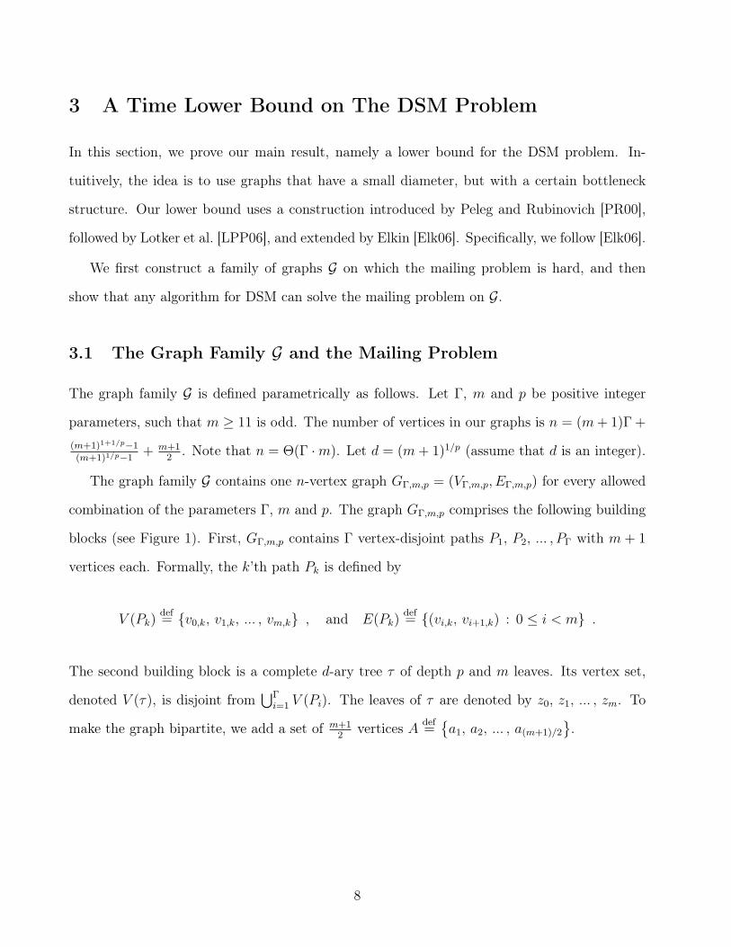
1 The graph family G, for d = 3. . . . . . . . . . . . . . . . . . . . . . . . . . . . . 9

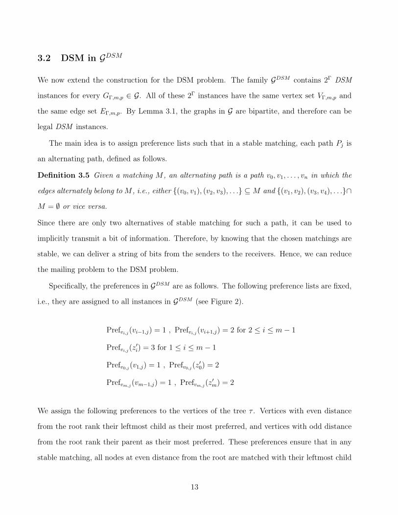
2 Left: preferences fixed at all 2Γ instances. The labels on the edges are the

respective preferences. Right: possible preferences assigned to v1,j. The actual

preferences in these nodes depend on the particular instance. . . . . . . . . . . . 14

3 The matchings along each path Pj are either the dashed edges or the bold edges. 15

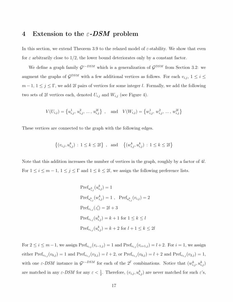
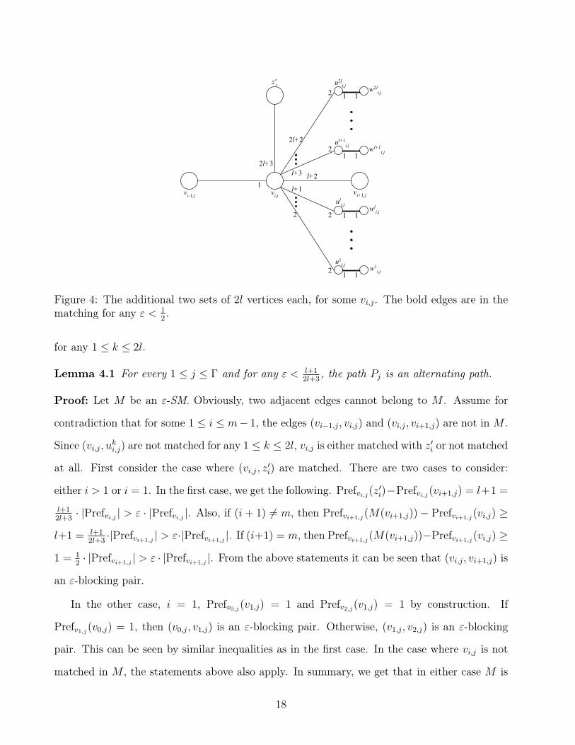
4 The additional two sets of 2l vertices each, for some vi,j. The bold edges are in

the matching for any ε < 12. . . . . . . . . . . . . . . . . . . . . . . . . . . . . . 18

iv

1 Introduction

Stable marriage, ever since it was invented by Gale and Shapley [GS62], is considered to be one of

the most interesting abstractions of markets: there are providers and customers (in the original

paper: colleges and applicants, or, more provocatively, men and women); each customer has a

ranking over the providers, and similarly each provider ranks the customers. Given a matching

M that matches each customer with a provider, we say that a customer-provider pair (i, j) is

blocking with respect toM if both i and j prefer each other to their matches underM . Clearly,

a blocking pair is a destabilizing element for M , because members of a blocking pair have an

incentive to “elope”, i.e., break M by matching to each other. Therefore, a desired fixed point

is a matching that does not induce any blocking pair; such a matching is said to be stable.

From the game-theoretic viewpoint, in stable matching (or stable marriage, as it is commonly

known, using the metaphor of men and women), unlike classical games, cooperation between

two players is a key ingredient. Consequently, the stability solution concept is robust against

the cooperation of any couple, in contrast to the Nash equilibrium solution concept, whose

motivation is that no lone player should have a reason to deviate from the solution state.

Beyond game theory, it is also interesting to note that stable matching has applications in

models without any hint of selfish agents, such as scheduling network switches [CGMP99].

Gale and Shapley proved that if the number of men is equal to the number of women, and if

the preference of each player is a total order over the players of the opposite sex, then a stable

marriage exists, and it can be found by a quadratic-time algorithm. Due to the many natural

applications and the non-trivial algorithmic essence of the problem, much work has followed.

The book by Gusfield and Irving [GI89] covers many variants of stable matching, such as

the case where preferences may include ties, or the case where some pairs are unacceptable

matches. Needless to say, most applications (like many scenarios considered in Game Theory)

are inherently distributed in nature, namely players act locally, and are not activated by a

central authority. It is therefore quite surprising that, to the best of our knowledge, until

1

now no one looked at the problem from the distributed computation point of view, where

communication between different players is accounted for. In this paper, we take a first step in

this direction. Specifically, modeling the input as a bipartite graph, where each edge represents

both a communication link and a possible match between its endpoints, we ask the question:

how much time (namely, communication rounds) is required to reach a stable matching?

More concretely, we consider the standard synchronous model [Pel00], where processors

communicate in synchronous rounds with their neighbors according to an underlying graph

G = (V,E): in each round, each processor can send a message to each of its neighbors. For the

distributed stable marriage problem (henceforth, DSM), the input to each node is a ranking of

its neighbors. It is not hard to see that no algorithm for DSM can terminate in less time than

required to cross the graph, i.e., the diameter of the graph. Intuitively, the reason is that input

at one end of the graph may determine the output at another end of the graph. It is also easy

to see that the following generic distributed algorithm can solve DSM: disseminate the whole

input to all nodes by “flooding,” and then let each node apply a fixed centralized algorithm

locally to find a global matching. This protocol is obviously unattractive as it just reduces the

distributed problem to n replicas of the centralized problem, where n = |V |. But there are

harder arguments against the generic protocol: even though no bit needs to traverse more than

diameter hops, the number of bits each node needs to receive is O(min(n2, |E| log n)), which

should result in high communication time in a realistic model.

To capture this phenomenon, in this paper we use the CONGEST model [Pel00], where a

message may contain up to B bits, for some parameter B of the model. We note that typically,

it is assumed that B = Θ(log n) (this means that each message may carry a constant number

of node IDs and variables of polynomial magnitude).

Our results. The main result in this paper is that in the CONGEST model, even for graphs

of diameter as small as Θ(log n), the number of rounds required to reach a stable matching

cannot be less than Ω(√n/B log n) in the worst case. The result holds even if we relax the

notion of stability in two natural ways, namely approximation and ε-stability. To explain these

2

relaxations, let us first define the standard notion of blocking pairs : a pair of players is called

blocking with respect to a given matching M if these two players prefer each other to their

matches under M . A matching is stable, then, if it does not induce any blocking pair. Our

lower bound holds even if we allow the algorithm to produce a matching which induces up to

O(√n) blocking pairs. The second relaxation is the concept of ε-stability, where we consider a

pair as ε-blocking only if by matching with each other they can improve the rank of their mate

by more than ε, relatively speaking (see a precise definition in Section 2). Our lower bound

holds for ε-stability as well.

We remark that the same technique extends to lower diameter graphs, at the price of

slightly weaker bounds: In the extreme case, we can show that there are graphs of diameter 6

that cannot be solved in fewer than Ω((n/B)1/3) rounds. For ε-stability, this lower bound holds

for diameter 10.

More related work. There are many papers devoted to Stable Marriage and its variants.

Gusfield and Irving survey the state of the art up to 1989 in their book [GI89]. Some compu-

tational hardness results for stable marriage were obtained later [HIMM02]. Recently there is

a renewed interest in the subject (e.g., a whole workshop was devoted to it [HIIM08] in 2008).

There are a few new directions of research. For example, motivated by organ transplants donor

scenarios, there are papers studying 3-way stable matchings: there are three sets of players,

usually thought of as men, women and dogs. In one variant each player ranks the players of

the other sets, and in another variant men rank only women, women rank only dogs, and dogs

rank only men. The goal is to match them into families of man, woman and dog.

A recent survey of the problem and its variants was published by Iwama and Miyazaki

[IM08]. Several fields of interest were discussed in this paper. One variant of the problem is

the Stable Roomates problem (denoted SR). In this problem there is a single set of even size of

players, and each player ranks all the others. The objective is to match the players into couples,

with a similar stability definition as in the SM problem. One application of algorithms for the

3

SR problem is pairings of players in chess tournaments [KLM99].

Another famous variant of SM is the Hospitals/Residents problem (denoted HR). In this

problem each hospital has a quota of residents, and the goal is to assign residents to hospitals

such that the matching is stable. This is a many-to-one extension of SM, in the sense that a

player of one team may be matched with more than one player of the other team. Irving et al.

[IMS00] studied this problem with ties in the preference lists.

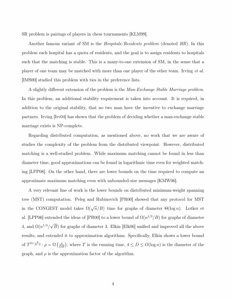
A slightly different extension of the problem is the Man-Exchange Stable Marriage problem.

In this problem, an additional stability requirement is taken into account. It is required, in

addition to the original stability, that no two man have the incentive to exchange marriage

partners. Irving [Irv04] has shown that the problem of deciding whether a man-exchange stable

marriage exists is NP-complete.

Regarding distributed computation, as mentioned above, no work that we are aware of

studies the complexity of the problem from the distributed viewpoint. However, distributed

matching is a well-studied problem. While maximum matching cannot be found in less than

diameter time, good approximations can be found in logarithmic time even for weighted match-

ing [LPP08]. On the other hand, there are lower bounds on the time required to compute an

approximate maximum matching even with unbounded-size messages [KMW06].

A very relevant line of work is the lower bounds on distributed minimum-weight spanning

tree (MST) computation. Peleg and Rubinovich [PR00] showed that any protocol for MST

in the CONGEST model takes Ω(√n/B) time for graphs of diameter Θ(log n). Lotker et

al. [LPP06] extended the ideas of [PR00] to a lower bound of Ω(n1/3/B) for graphs of diameter

4, and Ω(n1/4/√B) for graphs of diameter 3. Elkin [Elk06] unified and improved all the above

results, and extended it to approximation algorithms. Specifically, Elkin shows a lower bound

of T 2+ 2D−2 · ρ = Ω

(n

DB

), where T is the running time, 4 ≤ D ≤ O(log n) is the diameter of the

graph, and ρ is the approximation factor of the algorithm.

4

2 Model and Preliminaries

In this section we define the stable marriage problem, the CONGEST computational model,

and an auxiliary problem called the Mailing Problem. The Mailing Problem will be used to

prove our lower bounds in Sections 3 and 4.

Stable Marriage. We consider the following variant of the stable marriage problem, denoted

SM. The input consists of an undirected bipartite graph G = (V,E), and a preference list Prefv

for each node v ∈ V . Prefv is an ordered list of all neighbors of v. We write Prefv(u) = i for

neighbors u, v if u is the ith node in Prefv, and say that u is ranked i in v’s preference list.

Prefv(u) = 1 means that u is the neighbor most preferred by v. If u is not a neighbor of v, we

assume that Prefv(u) = ∞. A matching is a set of disjoint edges. Given a matching M with

(u, v) ∈ M , we denote M(v) = u and M(u) = v. If v is unmatched under M , we assume that

Prefv(M(v)) =∞. We can now define the key concept of blocking pairs.

Definition 2.1 A pair of nodes (u, v) is said to be blocking with respect to M if Prefv(u) <

Prefv(M(v)) and Prefu(v) < Prefu(M(u)).

We note that in the terminology of [GI89], our variant is the one with “unacceptable partners,”

because only pairs connected by an edge are eligible to the matching. Also, we allow the two

parts of the node set to be of unequal size, but for convenience, we do not allow “indifference”,

i.e., each node has a strict ordering over its neighbors.1 We generalize the notion of blocking

pairs as follows.

Definition 2.2 Let 0 ≤ ε ≤ 1. A pair of nodes (u, v) is said to be ε-blocking with respect to

M if Prefv(u) < Prefv(M(v))− ε|Prefv| and Prefu(v) < Prefu(M(u))− ε|Prefu|.

Note that a blocking pair according to Definition 2.1 is a 0-blocking pair according to Definition

2.2. Intuitively, the notion of ε-blocking pair formalizes the notion that stability is violated only

when there is a pair that can improve their matches “a lot” by matching to each other: a minor

improvement might just not worth the trouble.1The graph must be bipartite, or otherwise it may be the case that no stable marriage exists.

5

Finally, we can define a stable matching.

Definition 2.3 A matching M is said to be stable (resp., ε-stable for some 0 ≤ ε ≤ 1) if there

are no blocking pairs (resp., ε-blocking pairs) with respect to M .

A matching is a ρ-approximation to a stable marriage if it induces at most (1 − ρ)n blocking

pairs.

Computational Model. We use the standard synchronous message passing model called

CONGEST in [Pel00]. Briefly, in the CONGEST model, an undirected graph G = (V,E)

represents the system, where vertices represent processors and edges represent bidirectional

communication links. We use the terms “processor”, “node” and “vertex” interchangeably. We

denote |V | = n. Each vertex has a set of input variables, output variables, and some local

variables. An assignment to these variables is the local state of the processor. It is assumed

that each processor has a unique ID of O(log n) bits. At time 0, the environment sets the state of

the input variables, and the execution then proceeds in global synchronous rounds, where each

round consists of the following. Processors first send messages to their neighbors, then receive

messages sent to them in that round, and finally make a local computation. Each processor

can halt its computation. The protocol is terminated when all local nodes have halted. The

CONGEST model requires that no message is longer than B bits, for some given parameter B

(typically B = O(log n)).

In the Distributed Stable Marriage problems (denoted DSM and ε-DSM), the input to each

processor is its preference list, and the output at each processor is a register that either points

to its match or indicates that the processor is unmatched.

The Mailing Problem. To prove a lower bound on DSM, we shall use a lower bound on

the following variant of the Mailing Problem [PR00]. The input consists of two disjoint sets of

vertices S,R ⊆ V , referred to as the senders and the receivers, respectively. Each set contains b

vertices for some given integer b ≥ 1, and we denote S = s1, . . . , sb and R = r1, . . . , rb. For

1 ≤ j ≤ b, the sender sj has one input variable Xsj , and the receiver rj has one output variable

6

Xrj . An instance of the mailing problem is an assignment of one bit to the input variable of

each sender. The requirement is that when the protocol terminates, Xrj = Xs

j for all 1 ≤ j ≤ b.

7

3 A Time Lower Bound on The DSM Problem

In this section, we prove our main result, namely a lower bound for the DSM problem. In-

tuitively, the idea is to use graphs that have a small diameter, but with a certain bottleneck

structure. Our lower bound uses a construction introduced by Peleg and Rubinovich [PR00],

followed by Lotker et al. [LPP06], and extended by Elkin [Elk06]. Specifically, we follow [Elk06].

We first construct a family of graphs G on which the mailing problem is hard, and then

show that any algorithm for DSM can solve the mailing problem on G.

3.1 The Graph Family G and the Mailing Problem

The graph family G is defined parametrically as follows. Let Γ, m and p be positive integer

parameters, such that m ≥ 11 is odd. The number of vertices in our graphs is n = (m+ 1)Γ +

(m+1)1+1/p−1

(m+1)1/p−1+ m+1

2. Note that n = Θ(Γ ·m). Let d = (m+ 1)1/p (assume that d is an integer).

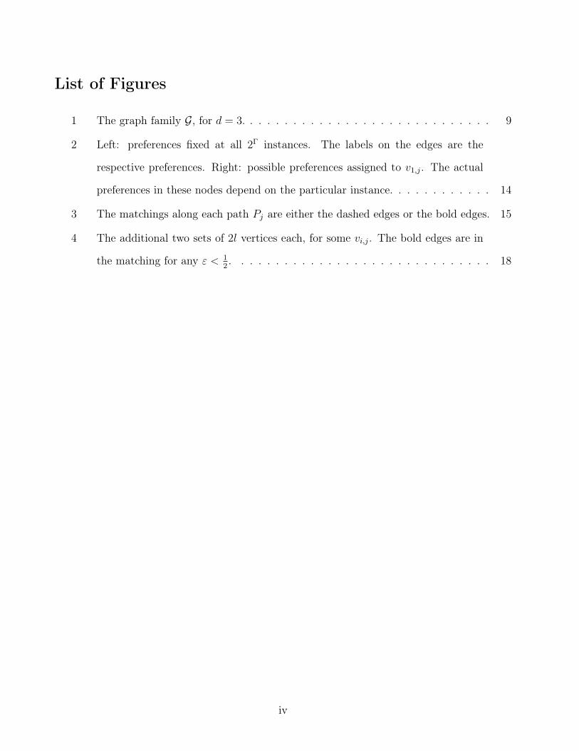
The graph family G contains one n-vertex graph GΓ,m,p = (VΓ,m,p, EΓ,m,p) for every allowed

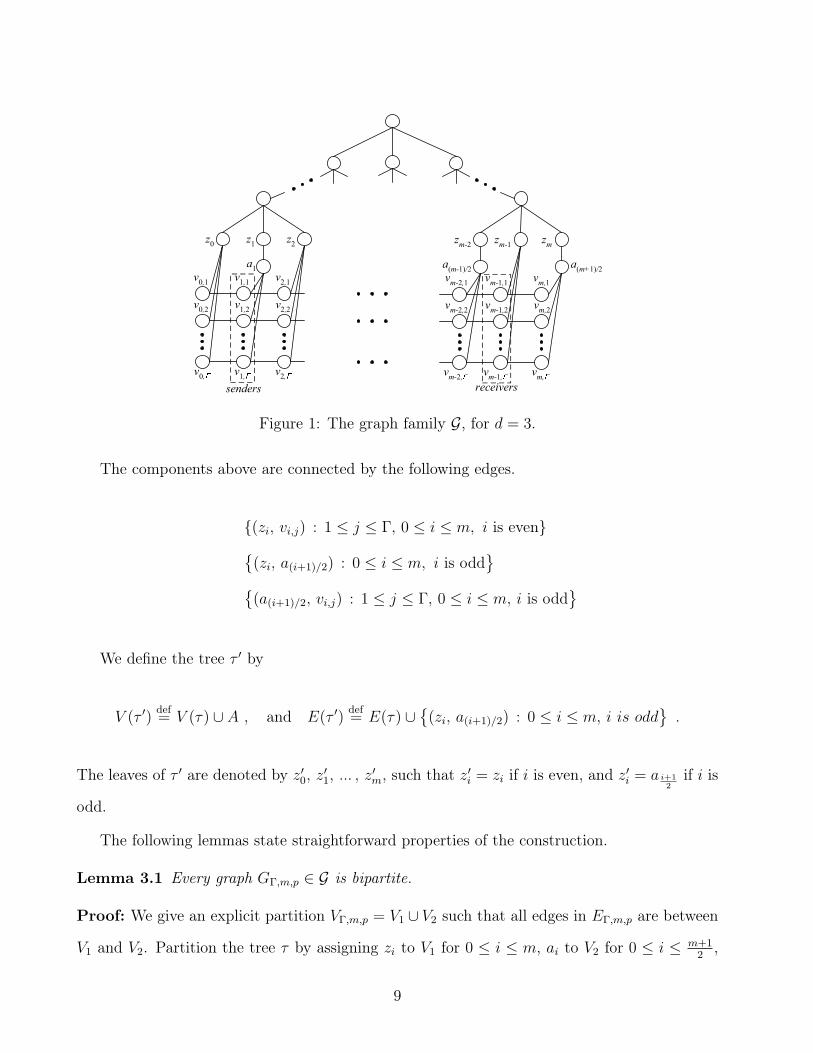
combination of the parameters Γ, m and p. The graph GΓ,m,p comprises the following building

blocks (see Figure 1). First, GΓ,m,p contains Γ vertex-disjoint paths P1, P2, ... , PΓ with m + 1

vertices each. Formally, the k’th path Pk is defined by

V (Pk)def= v0,k, v1,k, ... , vm,k , and E(Pk)

def= (vi,k, vi+1,k) : 0 ≤ i < m .

The second building block is a complete d-ary tree τ of depth p and m leaves. Its vertex set,

denoted V (τ), is disjoint from⋃Γ

i=1 V (Pi). The leaves of τ are denoted by z0, z1, ... , zm. To

make the graph bipartite, we add a set of m+12

vertices A def=a1, a2, ... , a(m+1)/2

.

8

v0,1

v1,1

v2,1 v

m-1,1vm,1

v0,2

v1,2

v2,2 v

m-1,2vm,2

v0,

v1,

v2, v

m-1,vm,

z0

z1

z2 z

m-1zm

a1 a

(m+1)/2

zm-2

a(m-1)/2

vm-2,1

vm-2,2

vm-2,

senders receivers

Figure 1: The graph family G, for d = 3.

The components above are connected by the following edges.

(zi, vi,j) : 1 ≤ j ≤ Γ, 0 ≤ i ≤ m, i is even(zi, a(i+1)/2) : 0 ≤ i ≤ m, i is odd

(a(i+1)/2, vi,j) : 1 ≤ j ≤ Γ, 0 ≤ i ≤ m, i is odd

We define the tree τ ′ by

V (τ ′)def= V (τ) ∪ A , and E(τ ′)

def= E(τ) ∪

(zi, a(i+1)/2) : 0 ≤ i ≤ m, i is odd

.

The leaves of τ ′ are denoted by z′0, z′1, ... , z′m, such that z′i = zi if i is even, and z′i = a i+12

if i is

odd.

The following lemmas state straightforward properties of the construction.

Lemma 3.1 Every graph GΓ,m,p ∈ G is bipartite.

Proof: We give an explicit partition VΓ,m,p = V1 ∪ V2 such that all edges in EΓ,m,p are between

V1 and V2. Partition the tree τ by assigning zi to V1 for 0 ≤ i ≤ m, ai to V2 for 0 ≤ i ≤ m+12

,

9

and assign the remaining vertices inductively, level by level. We divide the rest of the vertices

as follows. For every 0 ≤ i ≤ m and 1 ≤ j ≤ Γ, if i is even then vi,j ∈ V2, and otherwise

vi,j ∈ V1.

It remains to show that all edges connect nodes in V1 with nodes in V2. There are three

cases to consider. First, consider an edge (vi,j, vi+1,j). According to the chosen partition, if i is

even then vi,j ∈ V2 and vi+1,j ∈ V1, and otherwise vi,j ∈ V1 and vi+1,j ∈ V2. Second, consider

an edge (zi, vi,j). By construction of GΓ,m,p, this edge exists only if i is even, and we get that

vi,j ∈ V2 and zi ∈ V1. Finally, the case of an edge(ai+1/2, vi,j

)is analogous to the second case,

and the result follows.

Lemma 3.2 The diameter of a graph GΓ,m,p ∈ G is 2p+ 4.

Proof: We first show that the distance between any two vertices in the graph is not greater

than 2p + 4. Consider some vertices zi and vi,j. By construction of the tree τ , the distance

between zi and the root of the tree is p. The distance between vi,j and zi is either 1 or 2. Thus,

the total distance between vi,j and the root of the tree is not greater than p+ 2, and therefore

the distance between any two vertices in the graph is not greater than 2p+ 4. To see that the

diameter is not smaller than 2p + 4, note that the shortest path between v1,1 and vm,Γ goes

through the tree τ , and therefore the distance between them is 2p+ 4.

The main idea is to show that in every graph in G there is a sequence of cuts, such that

each bit has to cross all these cuts in order to be transfered from the senders to the receivers.

We then show that each of these cuts has low capacity, and therefore not “many” bits can cross

it simultaneously.

For this we need a few definitions, which are similar to those in [Elk06]. For 0 ≤ i ≤ m, we

denote by τ ′(i) the minimal subtree of τ ′ such that its set of leaves isz′i, z

′i+1, . . . , z

′m

. We

denote by V (τ ′(i)) the set of vertices of τ ′(i), and by E(τ ′(i)) its set of edges. For 1 ≤ i ≤ m,

we denote by Cuti the edges which are in the cut between V (τ ′(i)) and V (τ ′)\V (τ ′(i)). Note

that Cuti ⊆ E(τ ′).

10

The key property of the graphs in G, which follows directly from [Elk06], is stated next.

Lemma 3.3 Consider any deterministic protocol for the Mailing Problem running on GΓ,m,p,

where the senders are v1,1, v1,2, . . . , v1,Γ, and the receivers are vm−1,1, vm−1,2, . . . , vm−1,Γ. Let

t < m. Then the total number of configurations of local states of the receiver nodes after t steps

of the protocol is at most (2B+1 − 1)(t+4)·p·d.

Proof: Our construction is nearly identical to Elkin’s [Elk06], and our Lemma 3.3 is derived

from Lemma 3.4 in [Elk06]. Instead of reproducing the (complex) proof from [Elk06], let us

just review the differences here. First, in [Elk06] there is a single sender and single receiver

; and second, we introduced extra nodes ai that make sure that the graph is bipartite. The

extra nodes are clearly insignificant for the construction (they only increase the diameter by

an additive constant term). Moreover, the edges (zi′ , a(i′+1)/2) are not in any Cuti. Therefore,

using the same arguments as in the proof of Lemma 3.3 in [Elk06], we get that |Cuti| ≤ p · d

for any 1 ≤ i ≤ m. Now, we can apply Lemma 3.4 in [Elk06] and get that for the single-sender,

single-receiver problem, the total number of configurations of local states of the receiver node

after t steps of the protocol is at most (2B+1 − 1)t·p·d.

We note that the single sender z0 in [Elk06] is connected to all v0,j which are connected to

all our sender nodes v1,j. Also, the single receiver zm in [Elk06] (z′m in our graph) is connected

to all vm,j which are connected to all our receiver nodes vm−1,j. Obviously, a string at a node

can be sent to all nodes connected to it in a single step (one bit per node), and reversely, a set

of bits residing at different nodes can be collected in a single step by a node connected to all

of them. It follows that if after T steps there are at most q possible states at the single-sender,

single-receiver problem, then after T −4 steps there are at most q possible states at our version

of the problem.

Informally, Lemma 3.3 says that in every communication round before time m, at most

(B+1) ·p ·d information bits can arrive at the receiver nodes. Intuitively, this is the bandwidth

the tree τ can provide; after m time units, information may also arrive on the paths, potentially

11

delivering Γ ·B bits in each round.

We can now derive the following result which is the anchor for our lower bounds on DSM.

We do not attempt to optimize the constants here.

Theorem 3.4 Let m =(

np·B

)1/2− 12(2p+1) and let 0.8 < c ≤ 1 be a constant. Any deterministic

protocol for the mailing problem in GΓ,m,p that delivers correctly at least c ·Γ bits requires Ω (m)

rounds.

Proof: Suppose that a given protocol always delivers at least c · Γ bits in t steps for some

constant c > 0.8. Let R denote the set of all possible configurations of the receiver nodes

after t steps, for all possible inputs at the sender nodes. Since by assumption, at time t each

receiver configuration encodes i correct bits for some cΓ ≤ i ≤ Γ, a receiver configuration

may correspond to at most∑Γ

i=cΓ

(Γi

)sender configurations. Now, there are 2Γ possible sender

inputs, and hence it must be the case that

|R| ≥ 2Γ∑Γi=cΓ

(Γi

) ≥ 2Γ(ΓcΓ

)2Γ−cΓ

≥ 2cΓ

2ΓH(c)= 2Γ(c−H(c)) = 2Ω(Γ) . (1)

The first inequality follows from the explanation above.2 The second inequality follows from

the fact that∑n

i=k

(ni

)≤(

nk

)2n−k. The third inequality follows from the fact that for 0 < c < 1,(

ncn

)≤ 2nH(c), where H(·) is the entropy function. The last equality holds because H(c) < c for

c > 0.8.

Combining Eq. (1) with Lemma 3.3 which says that |R| ≤ (2B+1 − 1)t·p·d, we may conclude

that

(2B+1 − 1)t·p·d ≥ 2Ω(Γ) .

Recalling that d = m1/p and that Γ = Θ(n/m), we obtain t = Ω(n/(Bpm1+1/p)

). Using

m =(

np·B

)1/2− 12(2p+1) , the result follows.

2This is essentially the sphere-packing bound from the theory of error correcting codes, but for the reverseinequality.

12

3.2 DSM in GDSM

We now extend the construction for the DSM problem. The family GDSM contains 2Γ DSM

instances for every GΓ,m,p ∈ G. All of these 2Γ instances have the same vertex set VΓ,m,p and

the same edge set EΓ,m,p. By Lemma 3.1, the graphs in G are bipartite, and therefore can be

legal DSM instances.

The main idea is to assign preference lists such that in a stable matching, each path Pj is

an alternating path, defined as follows.

Definition 3.5 Given a matching M , an alternating path is a path v0, v1, . . . , vn in which the

edges alternately belong toM , i.e., either (v0, v1), (v2, v3), . . . ⊆M and (v1, v2), (v3, v4), . . .∩

M = ∅ or vice versa.

Since there are only two alternatives of stable matching for such a path, it can be used to

implicitly transmit a bit of information. Therefore, by knowing that the chosen matchings are

stable, we can deliver a string of bits from the senders to the receivers. Hence, we can reduce

the mailing problem to the DSM problem.

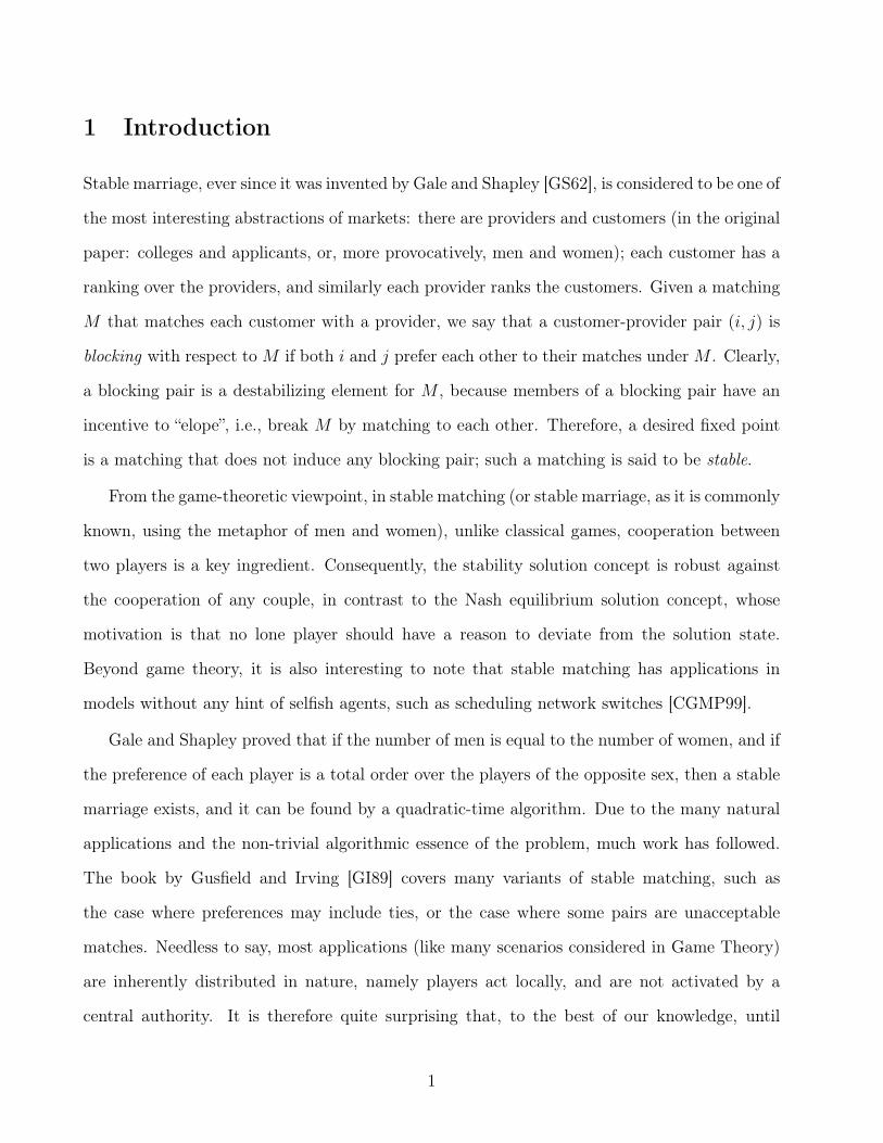
Specifically, the preferences in GDSM are as follows. The following preference lists are fixed,

i.e., they are assigned to all instances in GDSM (see Figure 2).

Prefvi,j(vi−1,j) = 1 , Prefvi,j

(vi+1,j) = 2 for 2 ≤ i ≤ m− 1

Prefvi,j(z′i) = 3 for 1 ≤ i ≤ m− 1

Prefv0,j(v1,j) = 1 , Prefv0,j

(z′0) = 2

Prefvm,j(vm−1,j) = 1 , Prefvm,j

(z′m) = 2

We assign the following preferences to the vertices of the tree τ . Vertices with even distance

from the root rank their leftmost child as their most preferred, and vertices with odd distance

from the root rank their parent as their most preferred. These preferences ensure that in any

stable matching, all nodes at even distance from the root are matched with their leftmost child

13

vi,j

vi+1,j

z'i

vi-1,j

1 2

3v0,j

v1,J

z'0

1

2

z'm

1

2

vm-1,j

vm,j

v1,j

v2,j

z'1

v0,j

1(2) 2(1)

3

Figure 2: Left: preferences fixed at all 2Γ instances. The labels on the edges are the respectivepreferences. Right: possible preferences assigned to v1,j. The actual preferences in these nodesdepend on the particular instance.

(other rankings in the tree are immaterial).

The variable part in the instances in GDSM is the preferences of the vertices v1,j, for 1 ≤

j ≤ Γ (see Figure 2). Each node v1,j may have Prefv1,j(v0,j) = 1 and Prefv1,j

(v2,j) = 2, or

Prefv1,j(v0,j) = 2 and Prefv1,j

(v2,j) = 1. There is exactly one DSM instance in GDSM for each of

the 2Γ possible combinations of v1,j , 1 ≤ j ≤ Γ.

We now state simple properties of the construction.

Lemma 3.6 Under any stable matching, the path Pj is an alternating path for all 1 ≤ j ≤ Γ.

Proof: Let M be a stable matching. Obviously, two adjacent edges cannot belong to M .

Assume for contradiction that for some 1 ≤ i ≤ m − 1, the edges (vi−1,j, vi,j) and (vi,j, vi+1,j)

are not in M . Also, assume that (vi,j, z′i) are matched. There are two cases to consider: either

i > 1 or i = 1. In the first case, (vi,j, vi+1,j) is a blocking pair. This can be seen from the

preference lists defined earlier. Since Prefvi+1,j(vi,j) = 1, vi+1,j prefers to be matched with vi

rather then with its current matching. Also, since Prefvi,j(vi+1,j) < Prefvi,j

(z′i), vi,j prefers to

be matched with vi+1,j rather then with its current matching. Hence, (vi,j, vi+1,j) is a blocking

pair. In the other case, i = 1, Prefv0,j(v1,j) = 1 and Prefv2,j

(1,j) = 1 by construction. If

Prefv1,j(v0,j) = 1, then (v0,j, v1,j) is a blocking pair. Otherwise, (v1,j, v2,j) is a blocking pair.

This is due to the simple fact that if Prefu(v) = Prefv(u) = 1, then (u, v) are matched in any

stable matching. In the case where vi,j is not matched in M , the statements above also apply.

In either case, we get that M is not stable, in contradiction with the assumption.

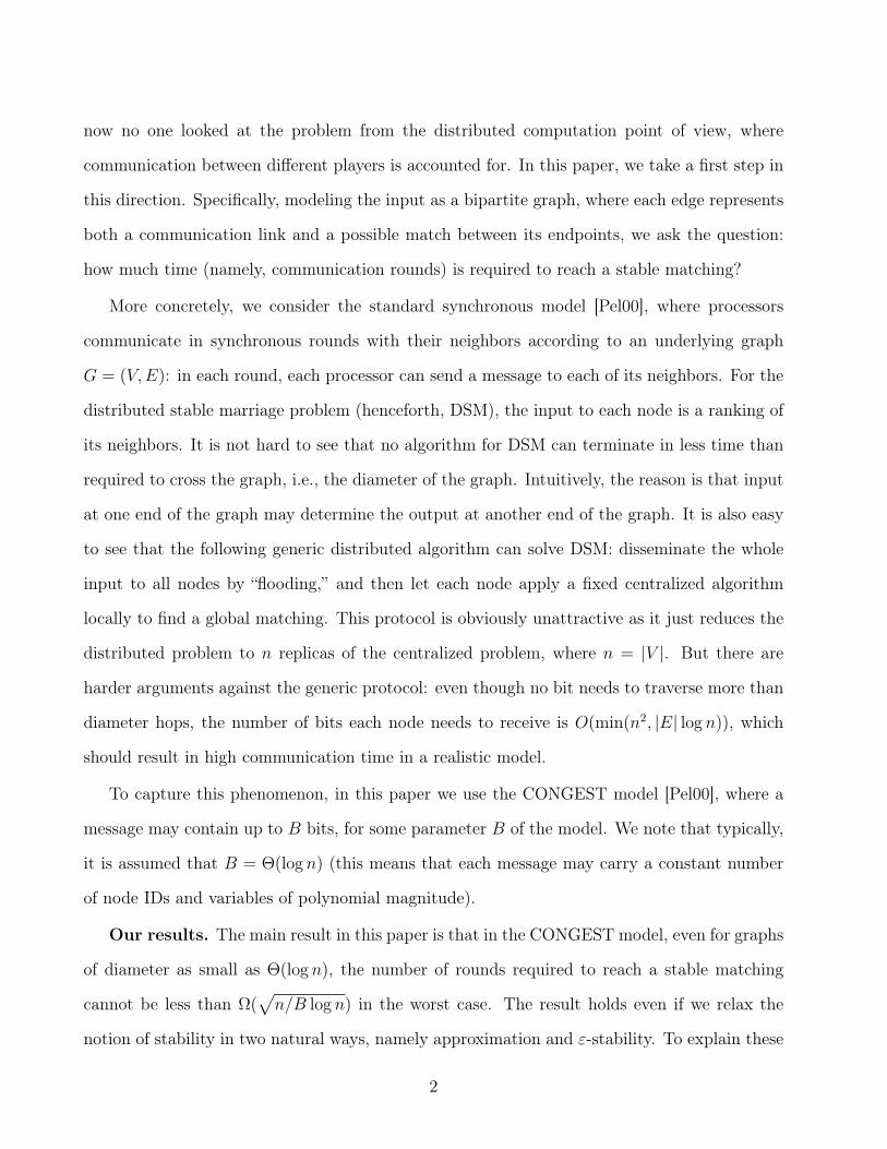
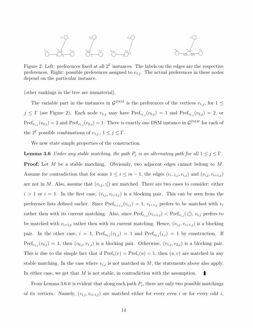
From Lemma 3.6 it is evident that along each path Pj, there are only two possible matchings

of its vertices. Namely, (vi,j, vi+1,j) are matched either for every even i or for every odd i,

14

v0,j

v1,j

v2,j

vm-1,j

vm,j

z'0

z'2

z'm-1

vm-2,j

z'1

z'm-2

z'm

Figure 3: The matchings along each path Pj are either the dashed edges or the bold edges.

0 ≤ i ≤ m− 1. The only thing that determines which of these two matchings is chosen, is the

preference list of v1,j. It is also evident that the matchings along each path do not depend on

the preferences assigned to the vertices of the tree.

Lemma 3.7 For every 1 ≤ j ≤ Γ, the preferences of v1,j determine the matching of all vertices

of Pj in any stable matching. Namely, if Prefv1,j(v0,j) = 1 then (vi,j, vi+1,j) are matched for

every even i, 0 ≤ i ≤ m− 1. Otherwise, if Prefv1,j(v2,j) = 1, (vi,j, vi+1,j) are matched for every

odd i, 0 ≤ i ≤ m− 1.

Proof: As argued earlier, if Prefv1,j(v0,j) = 1 then (v0, v1) are matched in any stable matching.

Since Pj is an alternating path, we get that (vi,j, vi+1,j) are matched for every even i, 0 ≤ i ≤

m − 1. Otherwise, (v1, v2) are matched in any stable matching. We get that (vi,j, vi+1,j) are

matched for every odd i, 0 ≤ i ≤ m− 1.

Corollary 3.8 Any deterministic algorithm for distributed stable marriage on graphs with di-

ameter D requires at least Ω(D) rounds.

Proof Sketch: Consider a graph that consists of a single path Pj of length D as above. By

Lemma 3.7, the match of vm−1 depends on Prefv1 , which is indistinguishable at vm−1 until time

D − 1.

Note that the lower bound of Corollary 3.8 does not hold for approximate stable matching:

a single blocking pair can flip the match at vm−1.

We can now prove our main result, namely a time lower bound on DSM.

Theorem 3.9 Consider any deterministic ρ-approximation for distributed stable marriage on

graphs with diameter D for D ∈ 6, 8, 10, . . ., and assume that ρ = 1 − o(1/√n). Then the

15

algorithm requires Ω(D +

(n

D·B

) 12− 1

2(D−3)

)communication rounds.

Proof: The diameter lower bound follows from Cor. 3.8. The second term of the lower bound

is proved by the following reduction of the Mailing problem on G to DSM on GDSM . Given

an input Xs1 , . . . , X

sΓ to the mailing problem in G ∈ G, we construct an instance of DSM

as follows. Preferences of all nodes except the sender nodes are fixed as described above.

We set the following preferences to the vertices v1,j. If Xsj = 1, then Prefv1,j

(v0,j) = 1 and

Prefv1,j(v2,j) = 2; and if Xs

j = 0, then Prefv1,j(v0,j) = 2 and Prefv1,j

(v2,j) = 1. This setting

is performed locally by the vertices v1,j, and therefore requires no distributed computation.

When the DSM algorithm terminates, each node knows its match. To complete the reduction

we define the output transformation by the rule that receiver nodes vm−1,j set Xrj = 1 if and

only if (vm−1,j, vm,j) is in the matching.

Suppose now that we have a ρ-approximate stable matching M in the graph, for some

ρ = 1 − o(1/√n). Then under M , there are at most (1 − ρ)n = o(

√n) blocking pairs, and

hence there are at least Γ − o(√n) paths Pj without any blocking pair, which means that at

least Γ− o(√n) paths Pj are alternating paths under M , and hence, by Lemma 3.7, the output

variables Xsj in their receiver nodes are correct. Now, recall that by our choice of m, we have

that Γ = Θ(n/m)√n, and hence the number of correct bits delivered using the reduction to

DSM is Γ(1− o(1)). In this case Theorem 3.4 applies, and we may conclude that the running

time of the algorithm under the specific graphs described there is Ω((

nD·B

) 12− 1

2(D−3)

).

By substituting D = log n, we get the following.

Corollary 3.10 Any deterministic ρ-approximation for DSM on graphs with diameter Θ(log n)

and ρ = o(1/√n), requires Ω

(√n

B·log n

)rounds.

By substituting D = 6, we get the following.

Corollary 3.11 Any deterministic ρ-approximation for DSM on graphs with diameter 6 and

ρ = o(1/√n), requires Ω

((nB

) 13

)rounds.

16

4 Extension to the ε-DSM problem

In this section, we extend Theorem 3.9 to the relaxed model of ε-stability. We show that even

for ε arbitrarily close to 1/2, the lower bound deteriorates only by a constant factor.

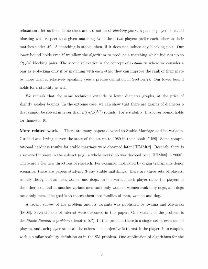
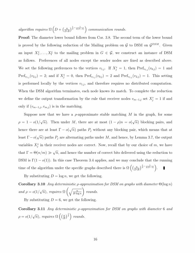
We define a graph family Gε−DSM which is a generalization of GDSM from Section 3.2: we

augment the graphs of GDSM with a few additional vertices as follows. For each vi,j, 1 ≤ i ≤

m− 1, 1 ≤ j ≤ Γ, we add 2l pairs of vertices for some integer l. Formally, we add the following

two sets of 2l vertices each, denoted Ui,j and Wi,j (see Figure 4).

V (Ui,j) =u1

i,j, u2i,j, ... , u

2li,j

, and V (Wi,j) =

w1

i,j, w2i,j, ... , w

2li,j

These vertices are connected to the graph with the following edges.

(vi,j, u

ki,j) : 1 ≤ k ≤ 2l

, and

(wk

i,j, uki,j) : 1 ≤ k ≤ 2l

Note that this addition increases the number of vertices in the graph, roughly by a factor of 4l.

For 1 ≤ i ≤ m− 1, 1 ≤ j ≤ Γ and 1 ≤ k ≤ 2l, we assign the following preference lists.

Prefwki,j

(uki,j) = 1

Prefuki,j

(wki,j) = 1 , Prefuk

i,j(vi,j) = 2

Prefvi,j(z′i) = 2l + 3

Prefvi,j(uk

i,j) = k + 1 for 1 ≤ k ≤ l

Prefvi,j(uk

i,j) = k + 2 for l + 1 ≤ k ≤ 2l

For 2 ≤ i ≤ m−1, we assign Prefvi,j(vi−1,j) = 1 and Prefvi,j

(vi+1,j) = l+ 2. For i = 1, we assign

either Prefv1,j(v0,j) = 1 and Prefv1,j

(v2,j) = l + 2, or Prefv1,j(v0,j) = l + 2 and Prefv1,j

(v2,j) = 1,

with one ε-DSM instance in Gε−DSM for each of the 2Γ combinations. Notice that (wki,j, u

ki,j)

are matched in any ε-DSM for any ε < 12. Therefore, (vi,j, u

ki,j) are never matched for such ε’s,

17

vi,j

vi+1,j

z'i

vi-1,j

u1i,j

uli,j

w1i,j

wli,j

1

2

l+1

u2li,j

ul+1i,j

w2li,j

2l+2

l+3

wl+1i,j

l+2

2l+3

1 1

1 1

2

2

1 1

1 1

2

2

Figure 4: The additional two sets of 2l vertices each, for some vi,j. The bold edges are in thematching for any ε < 1

2.

for any 1 ≤ k ≤ 2l.

Lemma 4.1 For every 1 ≤ j ≤ Γ and for any ε < l+12l+3

, the path Pj is an alternating path.

Proof: Let M be an ε-SM. Obviously, two adjacent edges cannot belong to M . Assume for

contradiction that for some 1 ≤ i ≤ m− 1, the edges (vi−1,j, vi,j) and (vi,j, vi+1,j) are not in M .

Since (vi,j, uki,j) are not matched for any 1 ≤ k ≤ 2l, vi,j is either matched with z′i or not matched

at all. First consider the case where (vi,j, z′i) are matched. There are two cases to consider:

either i > 1 or i = 1. In the first case, we get the following. Prefvi,j(z′i)−Prefvi,j

(vi+1,j) = l+1 =

l+12l+3· |Prefvi,j

| > ε · |Prefvi,j|. Also, if (i + 1) 6= m, then Prefvi+1,j

(M(vi+1,j))− Prefvi+1,j(vi,j) ≥

l+1 = l+12l+3·|Prefvi+1,j

| > ε·|Prefvi+1,j|. If (i+1) = m, then Prefvi+1,j

(M(vi+1,j))−Prefvi+1,j(vi,j) ≥

1 = 12· |Prefvi+1,j

| > ε · |Prefvi+1,j|. From the above statements it can be seen that (vi,j, vi+1,j) is

an ε-blocking pair.

In the other case, i = 1, Prefv0,j(v1,j) = 1 and Prefv2,j

(v1,j) = 1 by construction. If

Prefv1,j(v0,j) = 1, then (v0,j, v1,j) is an ε-blocking pair. Otherwise, (v1,j, v2,j) is an ε-blocking

pair. This can be seen by similar inequalities as in the first case. In the case where vi,j is not

matched in M , the statements above also apply. In summary, we get that in either case M is

18

not an ε-SM , in contradiction with the assumption.

Once again we get that along each path Pj there are only two possible ε-stable matchings.

The only thing that determines which of these two matchings is chosen, is the preference list of

v1,j. Therefore, the reduction of the mailing problem to the DSM problem can be applied for

the ε-DSM problem as well, for any ε < l+12l+3

.

We note that the additional vertices affect the lower bound attained for the mailing problem,

but do not affect its proof of correctness. This is due to the fact that these vertices are “dead-

ends”, i.e., they are not on any simple path between any sender and any receiver. Therefore,

they cannot contribute to any message passing between the senders and the receivers. We

conclude with the following extension of Theorem 3.9 to ε-stability.

Theorem 4.2 Consider any deterministic ρ-approximation for distributed ε-stable marriage

on graphs with diameter D for D ∈ 10, 12, 14, · · · , where ε < 1/2 is constant and ρ =

1− o(1/√n). Then the algorithm requires Ω

(D +

(n

D·B

) 12− 1

2(D−3)

)communication rounds.

We remark that corollaries 3.10 and 3.11 extend to ε-stability as well, for any ε < 1/2.

19

5 Algorithm for the ε-DSM problem

In this section, we show a distributed algorithm for the ε-DSM problem (DSM is just a special

case of ε-DSM). Our algorithm is a distributed version of an extension of Gale and Shapley

algorithm, augmented with a termination detection algorithm.

Let us first describe the basic algorithm. The nodes are divided into two sets, called active

and passive, according to the bipartition of the graph. Active nodes may only propose, and

passive nodes may only reject. The algorithm proceeds in double rounds. First, each rejected

active node proposes to the top node on its preference list (initially, all active nodes consider

themselves rejected, and their preferences are just the input). Then each passive node v that

has at least one proposal does the following. First, v sends a “reject” message to all proposers

except for the most preferred one (some active node u). If matching to u improves v’s status

by at least an ε fraction, then v rejects its current match, and otherwise v rejects u. Finally, v

rejects all nodes (including nodes that haven’t proposed to it) that cannot improve its status

by at least an ε fraction.

More formally, if a passive node v is currently matched with an active node u, then v sends

reject messages to all nodes u′ such that Prefv(u′) ≥ Prefv(u)−ε ·degreev, except those already

rejected by v. By degreev we denote v’s degree, i.e., the number of neighbors v has in the

graph. An active node u that receives a reject message from a passive node v, removes v from

its preference list. This way an active node u proposes only to passive nodes that appear to be

eligible matches to u at the time of the proposal. Algorithm 5.1 describes the action taken each

round by active and passive nodes. For an active node u, rejectu denotes a list of all passive

nodes which rejected u during the current round. For a passive node v, proposersv denotes a

list of all active nodes which proposed to v in the current round.

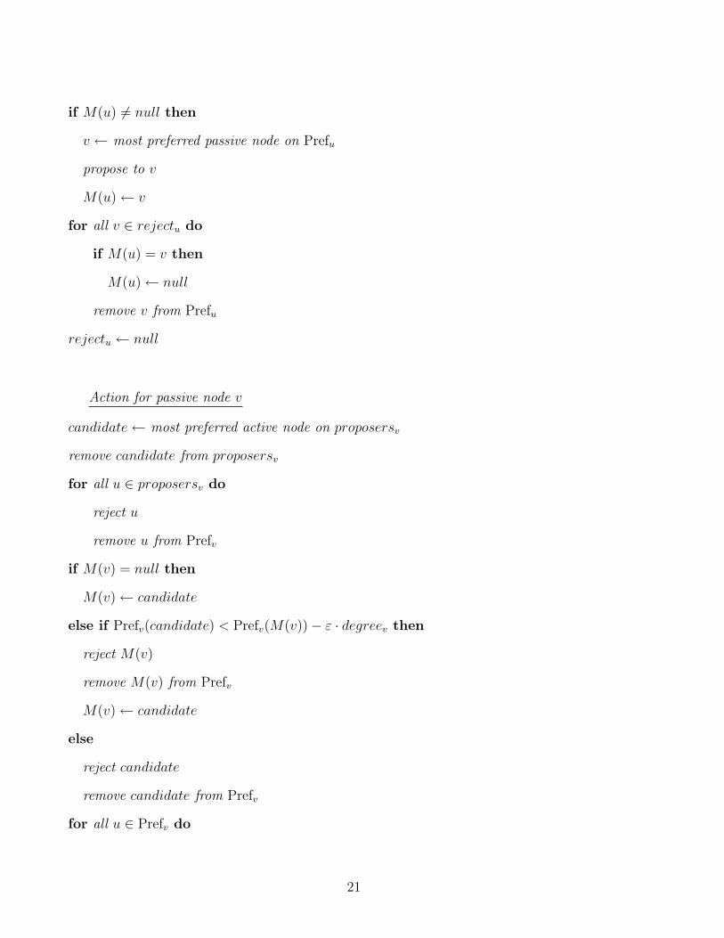
Algorithm 5.1 Distributed Stable Marriage

Action for active node u

20

if M(u) 6= null then

v ← most preferred passive node on Prefu

propose to v

M(u)← v

for all v ∈ rejectu do

if M(u) = v then

M(u)← null

remove v from Prefu

rejectu ← null

Action for passive node v

candidate← most preferred active node on proposersv

remove candidate from proposersv

for all u ∈ proposersv do

reject u

remove u from Prefv

if M(v) = null then

M(v)← candidate

else if Prefv(candidate) < Prefv(M(v))− ε · degreev then

reject M(v)

remove M(v) from Prefv

M(v)← candidate

else

reject candidate

remove candidate from Prefv

for all u ∈ Prefv do

21

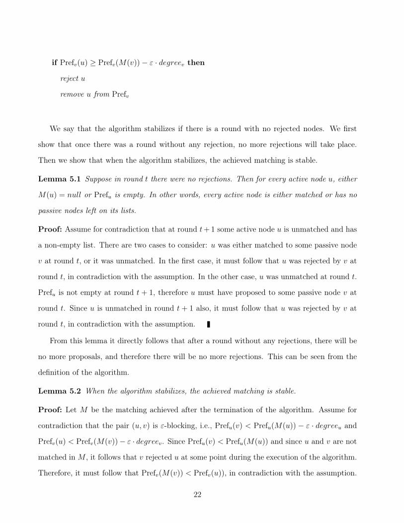
if Prefv(u) ≥ Prefv(M(v))− ε · degreev then

reject u

remove u from Prefv

We say that the algorithm stabilizes if there is a round with no rejected nodes. We first

show that once there was a round without any rejection, no more rejections will take place.

Then we show that when the algorithm stabilizes, the achieved matching is stable.

Lemma 5.1 Suppose in round t there were no rejections. Then for every active node u, either

M(u) = null or Prefu is empty. In other words, every active node is either matched or has no

passive nodes left on its lists.

Proof: Assume for contradiction that at round t+ 1 some active node u is unmatched and has

a non-empty list. There are two cases to consider: u was either matched to some passive node

v at round t, or it was unmatched. In the first case, it must follow that u was rejected by v at

round t, in contradiction with the assumption. In the other case, u was unmatched at round t.

Prefu is not empty at round t + 1, therefore u must have proposed to some passive node v at

round t. Since u is unmatched in round t + 1 also, it must follow that u was rejected by v at

round t, in contradiction with the assumption.

From this lemma it directly follows that after a round without any rejections, there will be

no more proposals, and therefore there will be no more rejections. This can be seen from the

definition of the algorithm.

Lemma 5.2 When the algorithm stabilizes, the achieved matching is stable.

Proof: Let M be the matching achieved after the termination of the algorithm. Assume for

contradiction that the pair (u, v) is ε-blocking, i.e., Prefu(v) < Prefu(M(u)) − ε · degreeu and

Prefv(u) < Prefv(M(v))− ε · degreev. Since Prefu(v) < Prefu(M(u)) and since u and v are not

matched in M , it follows that v rejected u at some point during the execution of the algorithm.

Therefore, it must follow that Prefv(M(v)) < Prefv(u)), in contradiction with the assumption.

22

Our idea to make this algorithm distributed is to add the following termination detection

mechanism: Let D be the diameter of the graph. We require each rejected node to broadcast

the fact that the protocol has not terminated yet, on a shortest-path tree. Thus, if O(D)

consecutive steps pass without any such broadcast received by a node v, v can safely conclude

that no rejected nodes are in the system, and it can therefore safely halt its local computations.

Finding the diameter of a graph is easy to do in diameter time (see, e.g., [Pel00]). We thus

obtain the following result.

Theorem 5.3 ε-DSM can be solved on any graph in time O(D + min(|E|, ε−1n)).

Proof: It takes O(D) time to find the value of D and to detect termination. Regarding the

stable marriage computation, note first that before stabilization of the matching, an active

node i proposes only to passive nodes that appear to be eligible matches to i at the time of

the proposal. Hence, at each round at least one proposal is not rejected, and therefore in each

round at least one passive node improves the rank of its match by at least a fraction ε. Since

each passive node can improve its match at most ε−1 times, it follows that the total number

of rounds until stabilization of the matching is bounded by O(ε−1n). In addition, note that

in each round before stabilization at least one fresh active node is rejected by a passive node,

and hence the total number of rounds before stabilization is also bounded by |E|. The result

follows.

For the exact case, we set ε = 1/(n + 1) and the running time is O(|E|). We remark

that even though in O(|E|) time one can disseminate the complete input to all nodes, the

algorithm above is more attractive for the following reasons. First, depending on the input, it

may terminate well before Ω(|E|) rounds have passed, while generic dissemination always takes

this much time. And second, the local computation required by the algorithm above is quite

trivial, while the generic dissemination algorithm requires each node to run the full centralized

stable-marriage algorithm.

23

6 Conclusion

In this paper we considered the Stable Marriage problem in a distributed model where messages

have bounded length. We showed that the number of communication rounds required to solve

the problem in this model cannot be smaller than Ω(√n/B log n), even if the graph has diameter

Θ(log n). On the other hand, our best upper bound for the problem is O(|E|) communication

rounds, or O(ε−1n) for ε-DSM. While we narrowed the gap, there is still work to do before our

original question is settled: what is the true distributed complexity of stable marriage?

24

References

[CGMP99] Shang-Tse Chuang, Ashish Goel, Nick McKeown, and Balaji Prabhakar. Matching

output queueing with a combined input output queued switch. IEEE Journal on

Selected Areas in Communications, 17(6):1030–1039, June 1999.

[Elk06] Micheal Elkin. An unconditional lower bound on the time-approximation tradeoff

for the minimum spanning tree problem. SIAM Journal on Computing, 36(2):463–

501, 2006.

[GS62] David Gale and L. S. Shapley. College admissions and the stability of marriage.

American Math. Monthly, 69:9–15, 1962.

[GI89] Dan Gusfield and Robert W. Irving. The Stable Marriage Problem: Structure and

Algorithms. MIT Press, Cambridge, MA, USA, 1989.

[HIIM08] Magnús M. Halldórsson, Rob Irving, Kazuo Iwama, and David

Manlove, editors. MATCH-UP: Matching Under Preferences, Reyk-

javík, Iceland, March 2008. Satellite workshop of ICALP 2008.

http://www.dcs.gla.ac.uk/research/algorithms/workshop/.

[HIMM02] Magnús M. Halldórsson, Kazuo Iwama, Shuichi Miyazaki, and Yasufumi Morita.

Inapproximability results on stable marriage problems. In LATIN ’02: Proc. 5th

Latin American Symp. on Theoretical Informatics, pages 554–568, London, UK,

2002. Springer-Verlag.

[Irv04] Robert W. Irving. Man-exchange stable marriage. University of Glasgow, Comput-

ing Science Department Research Report, TR-2004-177, 2004.

[IMS00] Robert W. Irving, David F. Manlove and Sandy Scott. The hospitals/residents

problem with ties. Proc. SWAT 2000, LNCS 1851, pages 259–271, 2000.

25

[IM08] Kazuo Iwama and Shuichi Miyazaki. A Survey of the Stable Marriage Problem

and Its Variants. Informatics Education and Research for Knowledge-Circulating

Society, 2008. ICKS 2008. International Conference on, pages 131–136, 17 Jan.

2008

[KMW06] Fabian Kuhn, Thomas Moscibroda, and Roger Wattenhofer. The price of being

near-sighted. In Proc. 17th Ann. ACM-SIAM Symposium on Discrete Algorithms,

pages 980–989, New York, NY, USA, 2006. ACM.

[KLM99] Eija Kujansuu, Tuukka Lindberg, and Erkki Makinen. The stable roommates prob-

lem and chess tournament pairings. Divulgaciones Matematicas, Vol. 7, No. 1, pages

19–28, 1999.

[LPP06] Zvi Lotker, Boaz Patt-Shamir, and David Peleg. Distributed MST for constant

diameter graphs. Distributed Computing, 18(6):453–460, 2006.

[LPP08] Zvi Lotker, Boaz Patt-Shamir, and Seth Pettie. Improved distributed approximate

matching. In Proc. ACM Symposium on Parallellism in Algorithms and Architec-

ture, pages 129–136, New York, NY, USA, 2008. ACM.

[Pel00] David Peleg. Distributed Computing: A Locality-Sensitive Approach. Society for

Industrial and Applied Mathematics, Philadelphia, PA, USA, 2000.

[PR00] D. Peleg and V. Rubinovich. Near-tight lower bound on the time complexity of

distributed MST construction. SIAM Journal on Computing, 30:1427–1442, 2000.

26

תקציר

דו צדדי לא גרףגרף התקשורת הוא, בבעיה זו. ית השידוך היציב המבוזרתי זו חוקרת את בעתזה

זוג צמתים אשר אינם משודכים , בהינתן שידוך של הצמתים. וכל צומת מדרג את שכניו, מכוון

שידוך נקרא . אחד לשני נקרא חוסם אם הם מעדיפים אחד את השני על פני השידוכים שלהם

.ב אם הוא לא משרה אף זוג חוסםיצי

עד , בכל סבב תקשורת על פני הקשתותצמתים מעבירים הודעות ביניהם, במודל המבוזר

, ביטים לכל היותרB הודעה יכולה להכיל כלאנו מראים שאם. אשר הם מוצאים שידוך יציב

)השידוך היציב דורש לפחות אזי כל אלגוריתם מבוזר אשר פותר את בעיית )nBn logΩ סבבי

)אפילו עבור גרפים בקוטר , תקשורת במקרה הגרוע ביותר )nO log , כאשרn הוא מספר

)החסם התחתון תקף גם אם אנו מאפשרים שהפלט יכיל , יתר על כן. הצמתים בגרף )nO זוגות

וגם במקרה בו זוג ייחשב חוסם רק אם הצמתים מעדיפים אחד את השני הרבה יותר, חוסמים

.מאשר את השידוכים שלהם

אביב–אוניברסיטת תל ש איבי ואלדר פליישמן"הפקולטה להנדסה ע

בעיית השידוך היציב המבוזרת בהנדסת חשמל" מוסמך אוניברסיטה"חיבור זה הוגש כעבודת גמר לקראת התואר

ידי–על

אלכסנדר קיפניס

מערכות–העבודה נעשתה במחלקה לחשמל

שמיר-בועז פת' בהנחית פרופ

ט"חשון תשס

אביב–אוניברסיטת תל ש איבי ואלדר פליישמן"הפקולטה להנדסה ע

בעיית השידוך היציב המבוזרת בהנדסת חשמל" מוסמך אוניברסיטה"חיבור זה הוגש כעבודת גמר לקראת התואר

ידי–על

אלכסנדר קיפניס

ט"חשון תשס