A NEW GENERATION OF HIGH STIFFNESS

ROTATIONAL MOULDING MATERIALS

HASHIM BHABHA

A thesis submitted in partial fulfilment of the

requirements of the Manchester

Metropolitan University for the degree of

Doctor of Philosophy

School of Healthcare Science

The Manchester Metropolitan University in

Collaboration with Rotomotive Ltd.

February 2015

Confidentiality Clause

This PhD thesis contains confidential data belonging to Rotomotive Ltd and Manchester

Metropolitan University (MMU). It should only be made available to the supervisory team,

examiners and authorised members of the Graduate School at MMU. Any publication or

duplication of this thesis, in partial or complete form, is prohibited. In order for patent

applications to be made relating to inventions that may arise from the work in this thesis, a two

year embargo period has been granted by the Research Degrees Committee at MMU. Therefore,

any inspection of this thesis by third parties requires the expressed permission of Hashim Bhabha,

Rotomotive Ltd. and MMU.

Abstract

Polyethylene (PE), particularly linear medium density PE (LMDPE), is the most widely used

thermoplastic in the rotational moulding (RM or rotomoulding) industry, possessing a balance

between melt flow characteristics and mechanical properties best suited to the RM process

relative to alternative thermoplastics. Reliance of the RM industry on LMDPE limits the application

envelope for manufacturers due to the inherently low modulus of the material; manufacturers

overcome this low modulus by increasing the wall thicknesses of their products which is costly

and energy intensive. The addition of filler particles to PE as a method of modulus enhancement

was considered a feasible alternative to increasing the wall thickness. The resulting composite

material could down gauge part thickness and potentially expand the application envelope of RM.

Phase 1 of this study observed the behaviour of RM grade PE’s with the introduction of filler

particles in order to double the modulus (namely garnet, sand, cenospheres or fly-ash and the

latter two combined). The PE/filler composites were mixed by dry blending or melt compounding,

moulded and mechanically tested in tensile, flexural and Charpy impact mode. The aim of

doubling the tensile modulus of rotomoulding grade PE was achieved by the melt compounded,

rotomoulded PE/fly-ash composites. The introduction of maleic anhydride grafted linear low

density polyethylene (MA-g-LLDPE) coupling agent also increased the modulus and tensile yield

stress of LMDPE with the addition of fly-ash. However, the beneficial melt flow rate and impact

toughness of PE decreased significantly with the addition of fly-ash. The latter was especially true

for rotomoulded samples.

As the RM industry typically uses finite element analysis (FEA) to numerically approximate the

stress or deflection of load-bearing parts, phase 2 of this study focused upon developing

numerical material properties for FEA of the new PE/fly-ash composites. Physical measurements

from compression tests on rotomoulded PE/fly-ash safety steps were close to FEA approximations

(confirming the practical value of the numerical materials data), except in the case of the unfilled

and highest filled PE samples. The significant differences observed between physical

measurements and FEA were probably due to complex factors such as the non-linear behaviour of

PE and the variation in wall thickness of rotomoulded parts, highlighting the importance of

properly understanding the finite element method (FEM) for RM.

Associated Publications

1. Bhabha, H. Using Finite Element Analysis as a Design Tool for Rotomoulded Parts, Manchester

Metropolitan University, Manchester, UK, British Plastics Federation Rotamoulding Tooling

Seminar Presentation, April 2013.

2. Bhabha, H. Using Finite Element Analysis for the Analysis of Rotomoulded Parts, Affiliation of

Rotational Moulding Organisations Newsletter, December 2013.

3. Bhabha, H. Liauw, C.M. Henwood, N.G. Taylor, H. Condliffe, J. Critical Factors Affecting the Use

of Finite Element Analysis For Rotomoulded Parts, Manchester Metropolitan University,

Manchester, UK, Rotomotive Ltd., Northampton, UK, Society of Plastics Engineers ANTEC (Annual

Technical) Conference Proceedings, April 2014.

Acknowledgements

First and foremost I would like to express my utmost thanks to my supervisory team, namely my

director of studies Dr. Chris Liauw, academic supervisor Dr. Howard Taylor and industrial

supervisor Dr. Nick Henwood. Without the guidance of my supervisory team, this PhD study

would not have been possible.

Furthermore, I am grateful to Mike Green of the polymer processing workshop at Manchester

Metropolitan University (MMU) and my industrial mentor Peter Luxford of Rotomotive Ltd for

training on various machinery such as the twin screw extruder, tensometer and water jet cutter.

I would also like to thank Gary Miller and Elaine Howarth of the analytical sciences department at

MMU who conducted scanning electron microscopy (SEM), energy dispersive x-ray (EDX) and

differential scanning calorimetry (DSC) on my behalf.

Moreover, I am thankful to the following people for assistance during the course of my studies:

Steve Davies of Crossfield Excalibur Ltd. for providing computer aided design (CAD) files of

the rotomoulded safety step.

David White of Excelsior Ltd. for providing the rotomoulded safety steps and access to

rotomoulding machinery.

Mark and Karen Drinkwater of JSC Rotational Ltd. for introducing me to numerous

members of the rotomoulding industry, including members of the British Plastics

Federation (BPF).

All of the technical staff members in the Faculty of Science and Engineering also deserve great

recognition for their help.

Finally, I would like to express the most heart-felt appreciation to my family and friends for

providing their moral support.

Declaration

I, Hashim Bhabha, hereby confirm that this work has not been and will not be submitted for any

other award apart from the award of Doctor of Philosophy from the Manchester Metropolitan

University. I also confirm that where other sources of information have been included, they have

been acknowledged correctly.

Signed: ………………….

H. Bhabha

Dated: ………………….

“Bismillah ir-rahman ir-rahim”

In the name of God, the most beneficent, the most merciful.

To Umi Jaan (Mother), Abba Jaan (Father) and all my family, with love.

Nomenclature

Abbreviation Description Units (where applicable)

PE Polyethylene -

LMDPE Linear medium density polyethylene -

HDPE High density polyethylene -

XLPE Cross-linked polyethylene -

PP Polypropylene -

PA Polyamide -

PC Polycarbonate -

MA-g-LLDPE Maleic anhydride grafted linear low density

polyethylene -

TSE Twin screw extruder/twin screw extrusion -

SEM Scanning electron microscopy/ Scanning

electron microscope -

RM Rotational moulding -

EDX Energy dispersive x-ray -

DSC Differential scanning calorimetry -

MFR Melt flow rate dg min-1

MPF Maximum packing fraction Value between 0-1

PSD Particle size distribution -

FE Finite element

FEA Finite element analysis -

FEM Finite element method -

CAD Computer aided design -

CAE Computer aided engineering

CNC Computer numerical control -

Contents

1. Introduction and Problem Statement 1

1.1 Aims and Objectives of the Study 2

2. Thesis Overview 4

3. Literature Review 6

3.1 The Rotational Moulding Process 6

3.2 Polymers Used for Rotational Moulding 8

3.2.1 Polyethylene 8

3.2.1.1 Polymerisation of ethylene 9

3.2.1.2 Development of chain branches in polyethylene 11

3.3 Particulate-Filled Polymers Used for Rotational Moulding 13

3.3.1 Particulate-filled polymer composite theory 14

3.3.1.1 Modulus of particulate-filled polymer composites 15

3.3.1.2 Yield stress of particulate-filled polymer composites 16

3.3.2 Origins of the filler particles 16

3.3.2.1 Silica sand 16

3.3.2.2 Almandine garnet 17

3.3.2.3 Fly-ash and cenospheres 17

3.3.3 Effects of filler reinforcements on polymer properties 17

3.3.4 Filler-matrix interaction (interfacial regions) 19

3.3.5 Filler-matrix coupling agents and filler particle surface treatments 19

3.4 Introduction to Finite Element Analysis 21

3.4.1 Partial differential equations 22

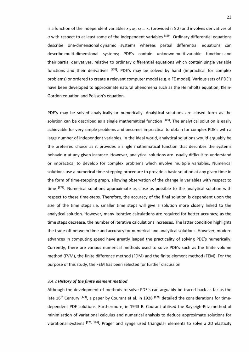
3.4.2 History of the finite element method 23

3.4.3 Theory and Requirements of the Finite Element Method 24

3.4.4 Finite element model development 25

3.4.4.1 Static linear-elastic analyses 26

3.4.4.2 Non-linear analyses 27

3.4.5 Finite element model refinement 28

3.5 Finite Element Analysis of Rotomoulded Parts 30

3.6 Summary of Literature Review 31

4. Experimental 35

4.1 Polyethylene Grades and Coupling Agent 35

4.1.1 Maleic anhydride grafted polyethylene (MA-g-LLDPE) 35

4.1.2 High density polyethylene (HDPE) 35

4.2 Candidate Filler Particles 36

4.3 Polyethylene and Filler Particle Characterisation 36

4.3.1 Determination of melt flow rate (MFR) 36

4.3.2 Estimation of filler particle maximum packing fraction (MPF) 37

4.3.3 Determination of filler particle densities 38

4.3.3.1 Sand, garnet and fly-ash 38

4.3.3.2 Cenospheres 38

4.3.4 Verification of filler particle size distribution 39

4.3.5 Determination of PE/filler composite densities 39

4.3.5.1 Densometer method 39

4.3.5.2 Ashing method 40

4.4 Blending of Filler Particles and Polyethylene to Form Composite Materials 41

4.4.1 Dry blended formulations 41

4.4.2 Two roll milled formulations 41

4.4.3 Twin screw extrusion compounded formulations 42

4.5 Moulding of PE/Filler Composites 43

4.5.1 Composite plaques prepared at Manchester Metropolitan University 43

4.5.2 Composite plaques prepared at Rotomotive Ltd. 44

4.5.3 Injection moulding of PE/fly-ash flexural test specimens 45

4.5.4 Bench-scale rotational moulding of PE/fly-ash rectangular test boxes 45

4.5.5 Commercial-scale rotational moulding of unfilled PE and PE/fly-ash safety steps 47

4.5.5.1 Unfilled PE safety steps 49

4.5.5.2 PE/fly-ash safety steps 50

4.6 Measurement of Mechanical Responses 50

4.6.1 Tensile Testing 50

4.6.1.1 Determination of tensile parameters from the raw data 50

4.6.2 Flexural testing 51

4.6.2.1 Determination of flexural parameters from the raw data 51

4.6.3 High temperature flexural testing of PE/fly-ash composites 53

4.6.3.1 Determination of flexural parameters from the raw data 54

4.6.4. Poisson’s ratio testing of PE/fly-ash composites 54

4.6.4.1 Determination of Poisson’s ratio from the raw data 54

4.6.5 Charpy impact testing of PE/fly-ash composites 56

4.6.6 Compression testing of rotomoulded safety steps 57

4.6.7 Tensile testing of safety step materials 58

4.6.8 Compression testing of safety step materials 59

4.6.8.1 Removal of machine compliance error 61

4.7 Surface Image Analysis of Rotomoulded PE/Fly-Ash Rectangular Box Test Mouldings 63

4.8 Scanning Electron Microscopy and Energy Dispersive X-Ray Analysis 65

4.8.1 Sample preparation 65

4.8.2 Scanning electron microscope and energy dispersive x-ray operating conditions 66

4.9 Differential Scanning Calorimetry 66

4.10 Finite Element Analysis of the Rotomoulded Safety Steps Sidewall Deflection 68

4.10.1 Finite element model development 69

4.10.2 Finite element model simplification and refinement 72

4.10.3 Finite element model analysis 75

5. Results and Discussion 77

5.1 Summary of Work 77

5.2 Characterisation of Materials for Composite Development 79

5.2.1 Effect of polymer structure 79

5.2.2 Dual polyethylene blends 79

5.2.2.1 Dry blended formulations 79

5.2.2.2 Twin screw extrusion compounded formulations 82

5.2.3 Key findings from the characterisation of materials for composite development 85

5.3 Analyses of Selected Candidate Fillers 85

5.3.1 Imaging of the candidate filler materials 86

5.3.1.1 Sieve analysis for construction of particle size distribution 88

5.3.2 Energy dispersive x-ray analysis 90

5.3.3 Density of the candidate filler materials 92

5.3.4 Determination of maximum packing fraction 92

5.3.4.1 Single filler systems 92

5.3.4.2 Dual filler systems 93

5.3.5 Key findings from analysis of the filler particles 95

5.4 Comparison of Composite Formation Processes for Large Particle Composites (Dry Blending of Pre-Mix versus Two Roll Mill Melt Blending and Moulding)

97

5.4.1 Estimation of tensile modulus and yield stress for filled polyethylene composites 102

5.4.2 Key findings from the comparison of composite formation processes 108

5.5 Use of Two Roll Mill Blending for Mixed Large/Small Particle Composites 109

5.5.1 Key findings from using the two roll mill to blend large/small particle composites 113

5.6 Evaluation of Twin Screw Extrusion Compounding for Production of Small Particle Composites

114

5.6.1 Key findings from using the twin screw extruder to blend small particle composites 118

5.7 Verification of Maleic Anhydride Coupling Agent Effect on Small Particle Composites Produced by Twin Screw Extrusion Compounding

119

5.7.1 Key findings from verifying the effect of Maleic Anhydride on PE/fly-ash composites 123

5.8 Comparison of Maleic Anhydride Coupling Agent Effect on HDPE and LMDPE Small Particle Composites Produced by Twin Screw Extrusion Compounding

123

5.8.1 Key findings from the comparison of Maleic Anhydride effects on HDPE and LMDPE fly-ash composites

128

5.9 Analysis of Rotationally Moulded Small Particle Composites 129

5.9.1 Rotomoulded rectangular box test mouldings 129

5.9.2 Rotomoulded safety steps 133

5.9.3 Key findings from the analysis of rotationally moulded small particle composites 141

5.10 High Temperature Flexural Testing of Injection Moulded PE/Fly-ash Composites 143

5.11 Cost Benefit Analysis of the Small Particle Composites for Rotational Moulding 144

5.12 Finite Element Analysis of Small Particle Composite Safety Step Sidewall Deflection 146

5.12.1 Specification of material properties for FE model development 146

5.12.1.1 Tensile properties and Poisson’s ratio 147

5.12.2 Further compression testing of small particle composite safety steps 149

5.12.3 Comparison of small particle composite safety step sidewall deflection with FEA 151

5.12.4 Formation of tensile-compression curve 156

5.12.5 Key findings from the finite element analysis of PE/fly-ash safety steps 158

5.12.6 Key considerations for the finite element analysis of rotomoulded parts 159

6. Conclusions 160

6.1 Mechanical Properties 160

6.2 Filler-Matrix Blending Technique 161

6.3 Polyethylene, Filler and Coupling Agent 161

6.4 Fillers - Effect of Bimodal Particle Size Distribution 162

6.5 Small Particle Composites – Properties in the Context of Rotational Moulding 162

6.6 Finite Element Analysis of Rotomoulded Small Particle Composites 163

6.7 Overall Recommendations 164

7. Further Work 166

8. References 168

Appendix 1 - 6 192

1

1. Introduction and Problem Statement

Rotational Moulding (RM) or rotomoulding is an effective method for the production of large

hollow components such as liquid storage tanks, kayaks and boats [1]. For the current repertoire of

applications, polyethylene (PE) is by far the most popular polymer used for RM. PE has the

mechanical properties, long-term melt stability and melt flow characteristics best suited to the

RM process, relative to alternative thermoplastics [2]. Furthermore, despite its low glass transition

temperature (Tg) PE can be easily converted into the powdered feedstock required for RM as it

can be produced by grinding at ambient temperature, without recourse to cryogenic grinding.

Arguably the most attractive factor favouring use of PE is its relatively low cost; PE is definitively

the cheapest polymer in the context of RM. However, the modulus of PE is inherently low.

Therefore, the wall thicknesses of rotomoulded products are increased to compensate for this low

modulus. Increasing the wall thickness is a common tactic for larger load-bearing articles such as

liquid storage tanks and silos, where manufacturers often over-thicken the walls to be confident

in part strength. Although practically justified, increasing the wall thickness of RM products uses

more material, slows production cycles and increases costs.

The latter limitations exemplified the requirement for “rotomouldable” materials with a higher

modulus. It was recognised that filler particles could provide the required modulus enhancement

to PE at relatively low expense in terms of toughness, processability and cost. Introducing

particulate fillers to reinforce polymers is a common technique amongst more popular plastics

manufacturing platforms such as injection or blow moulding. On the other hand, it is appreciated

that the number of studies regarding fillers for rotomoulding applications is relatively small [3-13];

rotomoulding is a relatively low pressure process which complicates the feasibility of using

particulate-filled polymers due to the reduction of melt flow properties (particularly at filler levels

where the reinforcement is most effective). Consequently, little research and development in

particulate-filled PE composite materials for RM has left a particularly large gap in knowledge.

Thus far, Arnaud [14], Hanna et al. [15] Kanokoriboon et al. [16] and Chang et al. [17] have conducted

the most noteworthy work on RM composites. However, this work was confined to using just one

filler material where large decreases in impact properties and melt flow rate (MFR) were

observed with relatively small increases in modulus and yield stress. Despite the latter, the option

of modifying the impact properties and melt flow rate (MFR) remained unexplored by Arnaud et

al [14-17]. Furthermore, studies by Ward et al. [18], Butora et al. [19], Lopez-Banuelos et al. [20], Yan et

al. [21] and Mhike [22] gave little consideration to important factors such as:

2

Using multiple fillers particles of various size and shape.

Varying the level of coupling agent.

Assessing different PE/filler blending techniques.

Blending various grades of PE for filler addition.

Furthermore, the RM industry typically uses finite element analysis (FEA) to approximate the

structural behaviour of load-bearing parts due to their geometry, material properties and load

scenario. The current body of research in FEA for rotomoulded parts is particularly small with only

one available reference from the Society of Plastics Engineers Annual Technical Conference

proceedings [23]. Therefore, a strong academic and industrial requirement exists to investigate FEA

for rotomoulded parts; the latter is especially true for load-bearing rotomoulded parts that are to

be produced using the proposed new particulate-filled PE composite. The combination of polymer

composite development and FEA is a novel venture in the field of rotomoulding.

1.1 Aims and Objectives of the Study

In order to address the knowledge gaps regarding the development of PE/filler composites for RM

and the FEA of rotomoulded parts, the aims and objectives of this PhD study are to:

1. Evaluate a selection of particulate fillers as reinforcement to RM grade PE in order to

double its tensile modulus – using Rotomotive’s powder blender and the compression

moulders at both Rotomotive Ltd. and MMU. MMU’s tensometer facility will be used for

mechanical testing.

2. Optimise the chosen composite system for performance and processability – using the

twin screw extrusion compounder and melt flow indexer (MFI) at MMU and the RM

machine at Excelsior Ltd. PE-filler interfacial modification will be controlled using chemical

coupling agents. The effect of the filler and coupling agent on the PE matrix will be

assessed using the SEM, DSC and EDX facilities at MMU.

3. Validate the numerical material property data of the new particulate-filled PE

composite materials using FEA – using SOLIDWORKS Simulation 2013 to compare FEA

with physical test results. Rotomoulded safety steps will be used as test subjects for the

proposed PE/filler composite materials and a computer aided design (CAD) file of the

safety steps 3D geometry will be used for FEA.

3 The primary goal of this study is to develop a particulate-filled PE composite material with at least

twice the modulus of PE. Therefore, the ultimate focus for phase 1 of this study is to investigate a

range of filler materials for addition to PE. Four fillers (sand, garnet, fly-ash, cenospheres and the

latter two combined) will be investigated in a matrix that comprises of maleanised 25 % wt. LLDPE

with 75 % wt. LMDPE (the former acts as a filler-matrix coupling agent). The filler content will be

varied using dry blending or melt compounding methods. The MA-g-LLDPE content will also be

varied using TSE melt blending. The possible benefits and limitations that the initial candidate

fillers, PE and coupling agent have to offer with regards to mechanical properties, rheological

effects and morphology will be explored during this phase. However, the earliest stages of phase

1 will be dedicated to the development of material test protocols.

The secondary goal of this study is to investigate the critical factors affecting the use of FEA for

rotomoulded parts made using the new particulate-filled PE composite materials. Therefore,

phase 2 of this study will focus upon developing a numerical database of material properties for

the new particulate-filled PE materials. Critical research questions that will be asked include, what

is FEA? How does it work? Moreover, are the mechanical properties of non-linear materials truly

representative? Rotomoulded safety steps made using PE/fly-ash composite PE materials will be

compression tested for sidewall deflection determination and compared with static linear-elastic

and non-linear FEA simulations (applying a force or displacement). Tensile tests will be conducted

to determine the mechanical properties required for FEA.

4

2. Thesis Overview

This study investigates the development of particulate-filled PE (PE/filler) composites to overcome

the low modulus of PE (the most common material used in the RM industry). The development of

numerical material property data to approximate the mechanical response of the PE/filler

composite materials using FEA software will also be explored. The latter software is commonly

applied to load-bearing RM parts to validate their mechanical performance before production.

Section 3 forms the literature review and is split into two sub-sections; PE/filler composite

material development and FEA. The first section introduces RM and the fundamentals of its

process. Furthermore, the rationale behind using PE for the vast majority of rotomoulded

products is also introduced; the relative popularity, manufacturing methods and property-

structure relationship of PE, in both the context of RM and the wider perspective, is discussed.

However, the low modulus of PE is a serious limitation to RM. Therefore, the use of particulate-

fillers to enhance the modulus of PE is discussed; fundamental polymer composite design theory

such as the effect of fillers on the matrix, the contribution of matrix-filler interaction and the

influence of filler particle surface treatments are explained. The second sub-section of the

literature review explores the history, mathematical theory and model development techniques

of the finite element method (FEM) for stress analysis, in order to provide a good understanding

of FEA software.

Section 4 details the experimental methods used for both the development of PE/filler composite

materials and FEA of rotomoulded PE/fly-ash safety steps. The novel image analysis technique

used for the determination of pinhole count and size distribution on the surfaces of rotomoulded

PE/fly-ash rectangular box test mouldings is also detailed within this section.

Section 5 presents and discusses the results obtained. The main findings of each investigation are

briefly summarised in the following paragraphs:

Twin screw extrusion (TSE) melt blended composites based on a mix of LMDPE, LLDPE grafted

with maleic anhydride coupling agent (MA-g-LLDPE or “maleanised” PE) and the finer filler

particles (i.e. fly-ash) produced compression mouldings with the best mechanical properties.

However, the improvements in tensile properties were accompanied by reduced impact

toughness at higher fly-ash loadings where the modulus enhancement was more prominent.

Equivalent composites based on a non-maleanised (analogue) LLDPE blended with LMDPE and fly-

5 ash had inferior mechanical properties. The highly-filled (70 % wt.) fly-ash LMDPE composites

displayed improvements in modulus with every increase MA-g-LLDPE investigated. The same was

true for equivalent HDPE composites however at lower MA-g-LLDPE loadings. Therefore, better

compatibility was observed between fly-ash particles and the LMDPE/MA-g-LLDPE blends. The

latter observations verify the claimed coupling activity of the MA-g-LLDPE with the finer fly-ash

particles. However, the addition of fly-ash severely decreased the melt flow rate (MFR) of the

resulting composites. Maximum packing fraction (MPF) tests confirmed that combinations of fly-

ash and cenospheres could boost filler volume fraction in PE. Conversely, the mechanical

response of the resulting composites was poor. During these trials it was concluded that the fly-

ash particles offered the best modulus enhancement. Rotomoulded maleanised PE/fly-ash

composites offered moduli comparable to that of higher density rotomoulding PE grades;

however this was observed at higher fly-ash loadings relative to compression moulded

equivalents. Furthermore, the part surface quality of rotomoulded PE decreased with the addition

of fly-ash. On the other hand, the variation in wall thickness of the rotomoulded PE safety steps

decreased considerably with the addition of fly-ash.

The numerical material parameters required for FEA of the PE/fly-ash composite materials were

the tensile modulus, stress at yield, Poisson’s ratio and full tensile stress-strain curves (for non-

linear analyses). Measured values of sidewall deflection for the rotomoulded PE/fly-ah safety

steps coincided reasonably well with most FEA approximations, confirming the practical value of

the material data from physical testing. Static linear-elastic FE models had considerably shorter

solution times in comparison to more complex non-linear FE models and yet were relatively

accurate. However, in some instances the significant differences between FEA and the actual

safety steps were probably due to the effect of various complex factors such as the non-linear

behaviour of PE and the variation in wall thickness of rotomoulded parts, exemplifying the

importance of properly understanding the FEM for rotomoulded parts.

Section 6 summarises the results of this study into a series of conclusions which are briefly

discussed in the previous paragraphs.

Section 7 identifies future work for this study; investigations exploring the creep response, zero-

shear MFR and processability of the PE/fly-ash composite materials are suggested.

6

3. Literature Review

3.1 The Rotational Moulding Process

RM involves the slow movement of powdered thermoplastic material within a heated metal

mould that is bi-axially rotated in an oven. The polymer powder first in contact with the mould

wall melts and sticks to the wall, sintering in to a continuous layer of polymer melt. Any residual

polymer powder in the mould then sticks to the initial sintered layer, increasing it in thickness

until all the powder has been consumed, leaving a coat of melt polymer around the interior wall

of the mould. The moulding is then then cooled down whilst slow rotation of the mould

continues. Once cooled completely, the mould is opened and the moulding removed.

Figure 1. RM process principles [24]

The rotomoulding production process consists of four main stages which are represented in

(Figure 1):

1. Charging - a predetermined mass (shot charge) of polymer (usually in powder form) is carefully

poured into a metal mould of the desired part. The average wall thickness of the finished

moulding is related to the mass of the charge. Currently, engineers use computer aided design

(CAD) software packages to calculate the desired part wall thickness.

7 2. Heating and Rotation - after charging the mould with the desired shot weight, the mould is

sealed and bi-axial rotation is initiated. The mould is then heated in an oven and the

consequent spreading of the powder ensures an even dispersion of the sintering powder

around the internals of the mould. After some time the polymer powder would have fully

melted and formed a homogenous layer effectively stuck to the internal mould surfaces.

3. Cooling - once all the polymer powder has amalgamated, the mould is cooled (whilst still

rotating) in an area containing air or water jets (or a combination of both). The reduction in

temperature from cooling solidifies the melt polymer; this cooling stage is kept as gradual as

possible as failure to do so can result in significant shrinkage or warpage of the moulding.

4. De-moulding - When the moulding has cooled sufficiently, rotation stops and the moulding is

carefully removed from the mould. Consequently, the mould is then ready for the next shot

charge and repeat of the process.

It is clear that rotomoulding is a unique polymer processing method in which there is no pressure-

induced flow of the polymer melt. The polymer powder melts when in contact with the surface of

the hot mould and sticks to it, forming a layer of polymer melt which then thickens as more

powder is melt-deposited on top of the initial layer. The particles of polymer powder in the melt

state have some elastic properties and are highly viscous in relation to a low molar mass liquid

such as water. Inter-diffusion of polymer between particles (resulting in sintering) is therefore

time dependent as the process is taking place under effectively zero-shear rate conditions. The

ability of the polymer chains to inter-diffuse under zero shear places unique demands on the

polymer. This factor together with the necessarily long cycle times (sometimes as long as 8 hours

for exceptionally large products such as liquid storage silos), which demand unusually high levels

of melt stability, places a limit on the range of materials suitable for rotomoulding.

The principles of RM have been implemented as far back as the Egyptian era, where it was used

for casting hollow ceramic objects [25]. However, the RM process was first applied to plastic

products during the 1950’s, mainly using polyvinylchloride (PVC) plastisols [26]. Having progressed

from a relatively simple method, RM is now a precisely controlled technique highly regarded by

designers of hollow load bearing structures [27]. Research and development in RM during the latter

half of the 20th century up to the present has led to notable improvements in component design

[28], process control [29], moulding techniques [30, 31] and materials. Linear medium density

polyethylene (LMDPE) is arguably the most popular thermoplastic for RM, with its use in most

applications. However, an industrial requirement for stiffer rotomoulded components led to the

8 development of HDPE and cross-linked polyethylene (XLPE) for RM applications. Specialist

applications in which the properties of PE do not suffice have led to the development of nylons

(PA), polycarbonates (PC) polypropylenes (PP) and even polylactides (PLA) for RM [32]. However,

the use of such thermoplastics is far from straightforward and requires tedious trial and error to

produce good quality mouldings with the desired profile of properties. The added expense and

processing difficulty of alternative polymers to PE for RM has led to limited developments of such

materials. To summarise, the benefits and limitations of rotomoulding are:

Advantages of rotomoulding

Good surface details and finishes.

Inexpensive prototype moulds.

Multi-layer laminate structures can be achieved.

Production moulds are considerably less expensive relative to blow moulding or injection

moulding.

Capable of moulding complex geometries.

Different sections of one product can be moulded within one tool.

Plastic or metal inserts can be integrated.

Disadvantages of rotomoulding

Material costs can be more expensive if pellets need to be ground into powder before

moulding.

Production times are longer in comparison to high pressure processes such as injection or

blow moulding.

Complicated or large parts can make the process labour intensive.

Polymers with high molar mass are unsuitable for rotomoulding.

Strengthening structures such as ribs are not easy to achieve.

Sudden changes in geometry are not easily achievable.

Consistency in terms of wall thickness is rarely achievable; mouldings are thicker in

corners.

3.2 Polymers Used for Rotational Moulding

3.2.1 Polyethylene

PE is arguably the most popular thermoplastic in the world, with applications in shopping bags,

bottles, children’s toys and even bullet proof vests [33, 34, 35]. PE represents the world’s number one

high volume thermoplastic in the modern age [36] mainly due to its low cost and versatility. For

9 example, in 2008 the annual global production of PE was approximately 80 million tonnes [37]. In

essence, PE has a simple structure composed of long monomer chains [38]. The monomer is

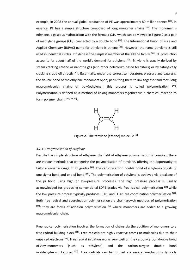
ethylene, a gaseous hydrocarbon with the formula C2H4 which can be viewed in Figure 2 as a pair

of methylene groups (CH2) connected by a double bond [39]. The International Union of Pure and

Applied Chemistry (IUPAC) name for ethylene is ethene [40]. However, the name ethylene is still

used in industrial circles. Ethylene is the simplest member of the alkene family [41]. PE production

accounts for about half of the world’s demand for ethylene [42]. Ethylene is usually derived by

steam cracking ethane or naphtha gas (and other petroleum based feedstock) or by catalytically

cracking crude oil directly [43]. Essentially, under the correct temperature, pressure and catalysis,

the double bond of the ethylene monomers open, permitting them to link together and form long

macromolecular chains of poly(ethylene); this process is called polymerisation [44].

Polymerisation is defined as a method of linking monomers together via a chemical reaction to

form polymer chains [45, 46, 47].

Figure 2. The ethylene (ethene) molecule [48]

3.2.1.1 Polymerisation of ethylene

Despite the simple structure of ethylene, the field of ethylene polymerisation is complex; there

are various methods that categorise the polymerisation of ethylene, offering the opportunity to

tailor a versatile range of PE grades [49]. The carbon-carbon double bond of ethylene consists of

one sigma bond and one pi bond [50]. The polymerisation of ethylene is achieved via breakage of

the pi bond using high or low-pressure processes. The high pressure process is usually

acknowledged for producing conventional LDPE grades via free radical polymerisation [51] while

the low pressure process typically produces HDPE and LLDPE via coordination polymerisation [52].

Both free radical and coordination polymerisation are chain-growth methods of polymerisation

[53]; they are forms of addition polymerisation [54] where monomers are added to a growing

macromolecular chain.

Free radical polymerisation involves the formation of chains via the addition of monomers to a

free radical building block [55]. Free radicals are highly reactive atoms or molecules due to their

unpaired electrons [56]. Free radical initiation works very well on the carbon-carbon double bond

of vinyl monomers (such as ethylene) and the carbon-oxygen double bond

in aldehydes and ketones [57]. Free radicals can be formed via several mechanisms typically

10 involving separate molecules to initiate the free radicals, these are called initiator molecules [58].

The latter molecules are a common initiation mechanism. However, there are several mechanisms

through which free radical polymerisation can be initiated. Depending on the initiation

mechanism, the active centre (centre of chain growth) will take a different form [59]. Free radical

polymerisation may be divided into three stages: chain initiation, chain propagation, and chain

termination [60]. Chain initiation is in two stages; during stage 1, one or two free radicals are

created using initiator molecules. During stage 2, the free radicals are transferred from the

initiator molecules to the monomers. For example, during the free radical

polymerisation of ethylene, the introduction of a free radical breaks the pi bond of ethylene and

two unpaired electrons rearrange to create a new active centre (similar to the initial free radical)

[61]. Following its generation, the initiating free radical adds non-radical ethylene monomers to

form chains (chain propagation). The free radical polymerisation of ethylene is possible only at

high temperatures and pressures (approximately 80-300 °C and 1500-3000 bar) [62]. However, the

polymerisation of vinyl chloride (for example) using the free radical method to produce

polyvinylchloride (PVC) does not require such extreme temperatures and pressures to succeed [63].

PE was first produced using a high-pressure free-radical polymerisation process by R. Gibson and

E. Fawcett at Imperial Chemical Industries (ICI) in 1933 [64]; it was discovered that ethylene (in its

natural gaseous form) could be converted into a white solid at high pressures and temperatures in

the presence of small levels of oxygen. The resulting polymerisation was a random uncontrolled

process producing a wide range of ethylene molecule sizes. However, it was possible to influence

the average molecule size (molecular weight) and the distribution of molecule size (molecular

weight distribution) around this average via control of the reaction conditions [65]. The PE chains

were highly branched (Section 3.2.1.2) at intervals of typically 20-50 carbon atoms using this high

pressure free radical polymerisation method. ICI named this new polymer “Polythene” and were

able to produce it at densities between approximately 0.91 - 0.93 g cm-3. It is known today as

LDPE and has its single biggest usage in blown film [66].

Coordination polymerisation involves the addition of monomers to a growing macromolecular

chain (Figure 3) through an organometallic active centre (usually metal chlorides or metal oxides);

the latter serves as a catalyst and is the central point of chain growth propagation [67, 68]. Catalysts

for the coordination polymerisation of ethylene were first developed in the early 1950’s; in 1951

[69] the Philips Petroleum Company developed catalysts prepared by depositing chromium

trioxide on silica [70] (Philips catalysts). Furthermore, in 1953 K. Ziegler and G. Natta [71] developed

catalysts based on titanium tetrachloride and an aluminium co-catalyst such as

methylaluminoxane [65] (Ziegler-Natta catalysts). The Philips and Ziegler-Natta (ZN) catalysts

11 permitted the polymerisation of ethylene (via coordination polymerisation) at much lower

pressures than the free radical polymerisation process developed by ICI; the PE produced had a

higher modulus than any previously developed PE grade, with a density range of about 0.940 -

0.970 g cm-3. The increased modulus and density were due to a significantly lower level of chain

branching; the microstructure consisted of straight (linear) ethylene chains with a narrow

molecular weight distribution and a high average chain length. The latter was classed as HDPE.

Metallocene catalysts first developed by Sinn and Kaminksky in 1980 [72] gave even better control

over the microstructure of PE than Philips or ZN catalysts [73]. Generally speaking, the

polymerisation method forms the distinction between LDPE, MDPE or HDPE.

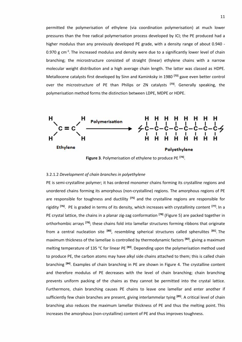
Figure 3. Polymerisation of ethylene to produce PE [74].

3.2.1.2 Development of chain branches in polyethylene

PE is semi-crystalline polymer; it has ordered monomer chains forming its crystalline regions and

unordered chains forming its amorphous (non-crystalline) regions. The amorphous regions of PE

are responsible for toughness and ductility [75] and the crystalline regions are responsible for

rigidity [76]. PE is graded in terms of its density, which increases with crystallinity content [77]. In a

PE crystal lattice, the chains in a planar zig-zag conformation [78] (Figure 5) are packed together in

orthorhombic arrays [79]; these chains fold into lamellar structures forming ribbons that originate

from a central nucleation site [80], resembling spherical structures called spherulites [81]. The

maximum thickness of the lamellae is controlled by thermodynamic factors [82], giving a maximum

melting temperature of 135 oC for linear PE [83]. Depending upon the polymerisation method used

to produce PE, the carbon atoms may have alkyl side chains attached to them; this is called chain

branching [84]. Examples of chain branching in PE are shown in Figure 4. The crystalline content

and therefore modulus of PE decreases with the level of chain branching; chain branching

prevents uniform packing of the chains as they cannot be permitted into the crystal lattice.

Furthermore, chain branching causes PE chains to leave one lamellar and enter another if

sufficiently few chain branches are present, giving interlammelar tying [85]. A critical level of chain

branching also reduces the maximum lamellar thickness of PE and thus the melting point. This

increases the amorphous (non-crystalline) content of PE and thus improves toughness.

12

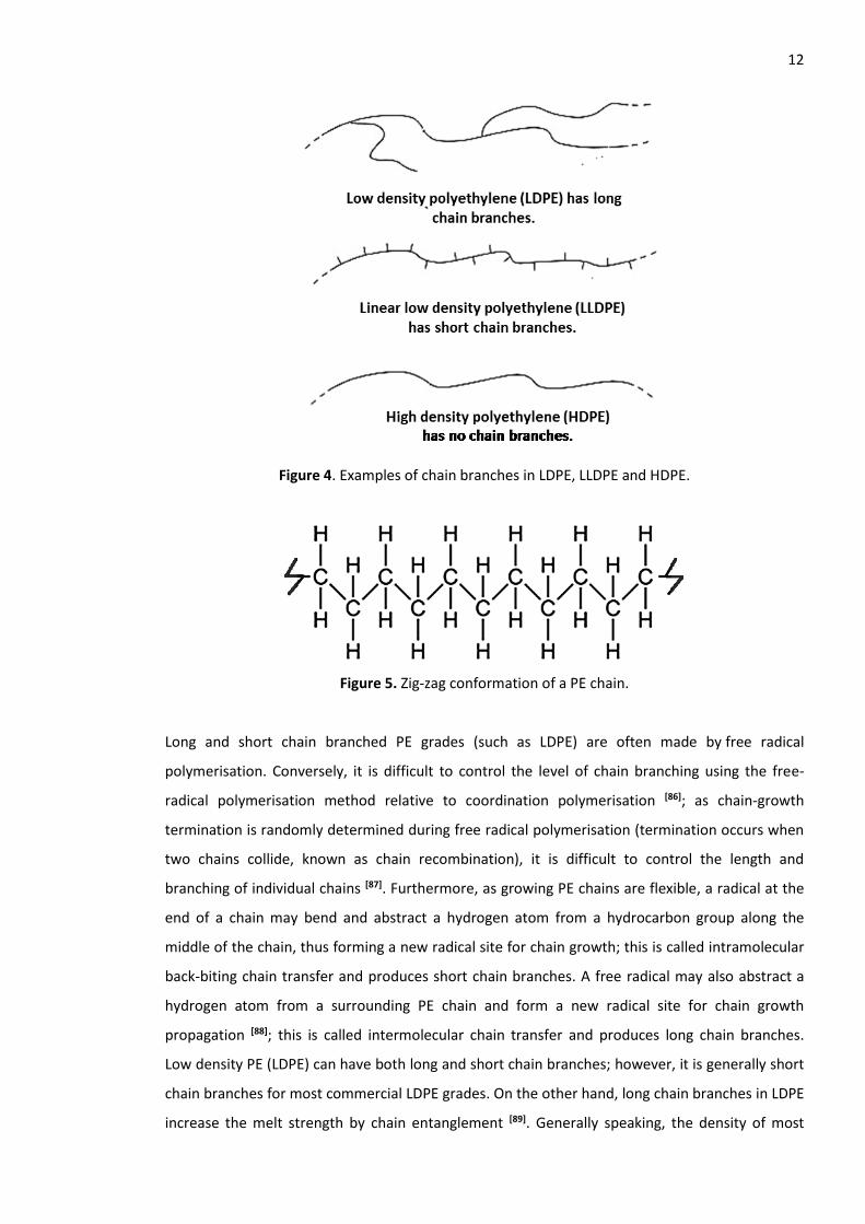
Figure 4. Examples of chain branches in LDPE, LLDPE and HDPE.

Figure 5. Zig-zag conformation of a PE chain.

Long and short chain branched PE grades (such as LDPE) are often made by free radical

polymerisation. Conversely, it is difficult to control the level of chain branching using the free-

radical polymerisation method relative to coordination polymerisation [86]; as chain-growth

termination is randomly determined during free radical polymerisation (termination occurs when

two chains collide, known as chain recombination), it is difficult to control the length and

branching of individual chains [87]. Furthermore, as growing PE chains are flexible, a radical at the

end of a chain may bend and abstract a hydrogen atom from a hydrocarbon group along the

middle of the chain, thus forming a new radical site for chain growth; this is called intramolecular

back-biting chain transfer and produces short chain branches. A free radical may also abstract a

hydrogen atom from a surrounding PE chain and form a new radical site for chain growth

propagation [88]; this is called intermolecular chain transfer and produces long chain branches.

Low density PE (LDPE) can have both long and short chain branches; however, it is generally short

chain branches for most commercial LDPE grades. On the other hand, long chain branches in LDPE

increase the melt strength by chain entanglement [89]. Generally speaking, the density of most

13 short chain branched PE grades varies between 0.91-0.939 g cm-3 [90]; this range in density defines

low to medium density PE (MDPE). When there is little (or no) chain branching present in PE, it is

graded as linear PE or HDPE. Linear PE is much stiffer than branched PE as linear chains can pack

together into a crystal lattice more effectively, resulting in higher crystallinity and density [91].

However, branched PE is tougher and easier to produce [92]. Linear PE is made using the

coordination polymerisation method. Coordination polymerisation has a significant impact on the

structural properties of vinyl polymers such as PE relative to equivalent polymers produced by

free radical polymerisation; the polymers tend to be linear (have little or no chain branching) and

have a considerably higher molar mass (indicating the chain lengths are longer) [93]. Polymers

produced by coordination polymerisation are also stereoregular, indicating the spatial

configuration of the monomers is consistent (such as PE, Figure 3). Ordered monomer

configurations introduce crystallinity in otherwise amorphous polymers [52]. However, high

crystalline content is not always desirable; some controlled branching during coordination

polymerisation is required for better control over density to produce linear MDPE (LMDPE), LLDPE

and even very low density PE (VLDPE). For example, copolymerising ethylene monomers with an

alkyl-branched comonomer (via coordination polymerisation) produces LLDPE which has short

branches. The latter exemplifies that coordination polymerisation may also be used if short chain

branching is required.

3.3 Particulate-Filled Polymers Used for Rotational Moulding

In 2012, the UK consumed approximately 15 % of the total European resin demand for RM [94],

making it the one of the largest producers of rotationally moulded products in Europe. One

obstacle to the growth of the rotational moulding industry lies in its dependence on PE to meet

the performance demands of end users. PE is relatively thermally stable and so is well suited to

rotomoulding but its stiffness is relatively low. Therefore, it would be desirable to modify PE in

such a way that its properties are enhanced [14]. One feasible solution to this is a composite

material composed pre-dominantly of PE. A successful composite material can be defined as a

combination of two or materials that results in better properties than those of the individual

components used alone [95]. Due to the economic and practical advantages of bulk thermoplastics

such as PE, the addition of particulate materials (or filler particles) has proved to be an effective

method of stiffness enhancement. The plastics industry is one of the most cost competitive

markets for materials engineering, particularly for mineral suppliers who rely heavily on their

products to enhance existing polymers [96]. Filler materials give practically infinite possibilities for

thermoplastics; consider the numerous combinations of thermoplastics with an equally large

selection of fillers such as talc particles or carbon fibres [97, 98]. The attributes of particulate-filled

14 polymer composite materials could be low cost, decreased density (if hollow particles are used),

increased strength or improved thermal conductivity [99]. It is known that the addition of mineral

fillers to PE (and all thermoplastics with a glass transition temperature (Tg) below room

temperature) results in a higher modulus [100].

Whilst one of the primary roles of filled polymers is to reduce costs, this role is normally

superseded by the reinforcing effects or reduction in mould shrinkage. Furthermore, the

introduction of fillers influences end product properties such as density and processability. Ideally,

particulate-filled PE composite materials for RM should as much as possible maintain the

toughness, processing window and relative economy of PE. Many studies have confirmed the

introduction of particulate fillers to PE can enhance mechanical properties and dimensional

tolerances [101, 102]. However, increasing the stiffness of PE via the addition of filler particles may

reduce toughness. Furthermore, the addition of filler particles increases the melt viscosity of PE,

hindering its flow during processing [103]. Therefore, it is recognised that the deterioration of

properties in particulate-filled PE composites may also depend on the level of filler addition. Such

composite materials for RM demand a good assessment of the inevitable compromise between

stiffness, toughness and melt flow properties with the addition of filler particles.

The effectiveness of particulate-filled polymer composites relative to unfilled polymers is

generally due to the base polymer properties, filler particle properties, level of filler particle

addition, strength of filler-matrix interaction and manufacturing methods [21]. To gain a true

appreciation of the influence each variable has on filled PE composites, it is necessary to

understand the theory of particulate-filled polymer composites and the effects of filler

reinforcement on the properties of polymers.

3.3.1 Particulate-filled polymer composite theory

In scientific literature, a vast number of theoretical models are available to approximate the effect

of particulate fillers on the modulus and yield stress of thermoplastics [104]. Generally, the most

noticeable difference to thermoplastics with the addition of filler particles is the increase in

modulus (if the filler particles are of higher modulus than the matrix) [105]; this is due to the

constraints imposed on the movement of the matrix by the filler particles (i.e. the matrix

ligaments are sandwiched between the filler particles). The latter is generally due to a variety of

factors such as filler particle size, shape, distribution, volume fraction (Vf) and interaction with the

polymer matrix. The interaction of untreated filler particles with the polymer matrix (i.e. no

coupling or dispersion agents are used, see Section 3.3.5) is mainly due to thermal contraction of

the polymer around the filler particles when the composite is cooled. The latter generates a

frictional force between the filler particle and the matrix that also constrains the movement of

15 the matrix. On the other hand, if the filler particles are treated with a chemical coupling agent to

promote better matrix-filler interaction, the probable increase in filler-matrix interaction will also

increase the modulus.

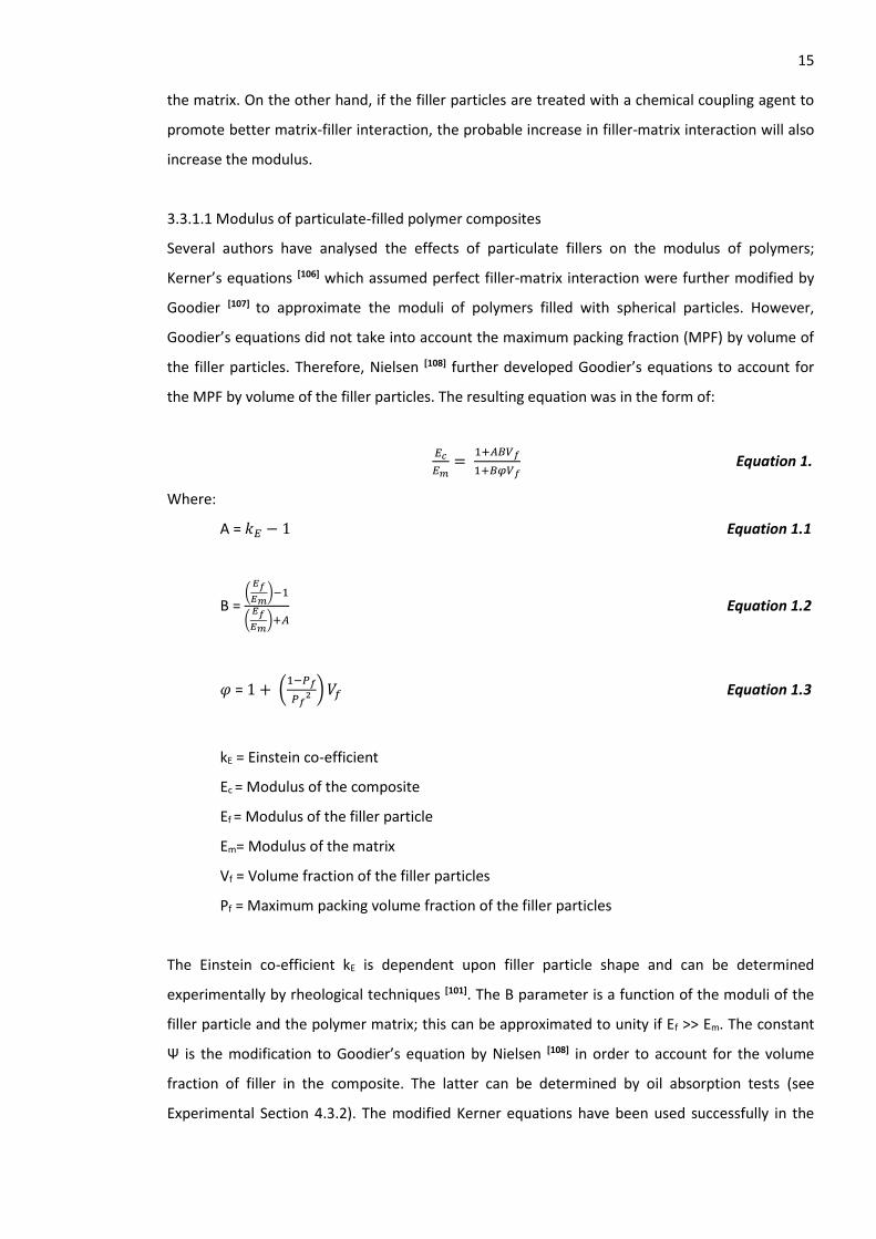
3.3.1.1 Modulus of particulate-filled polymer composites

Several authors have analysed the effects of particulate fillers on the modulus of polymers;

Kerner’s equations [106] which assumed perfect filler-matrix interaction were further modified by

Goodier [107] to approximate the moduli of polymers filled with spherical particles. However,

Goodier’s equations did not take into account the maximum packing fraction (MPF) by volume of

the filler particles. Therefore, Nielsen [108] further developed Goodier’s equations to account for

the MPF by volume of the filler particles. The resulting equation was in the form of:

𝐸𝑐

𝐸𝑚=

1+𝐴𝐵𝑉𝑓

1+𝐵𝜑𝑉𝑓 Equation 1.

Where:

A = 𝑘𝐸 − 1 Equation 1.1

B = (

𝐸𝑓

𝐸𝑚)−1

(𝐸𝑓

𝐸𝑚)+𝐴

Equation 1.2

𝜑 = 1 + (1−𝑃𝑓

𝑃𝑓2 ) 𝑉𝑓 Equation 1.3

kE = Einstein co-efficient

Ec = Modulus of the composite

Ef = Modulus of the filler particle

Em= Modulus of the matrix

Vf = Volume fraction of the filler particles

Pf = Maximum packing volume fraction of the filler particles

The Einstein co-efficient kE is dependent upon filler particle shape and can be determined

experimentally by rheological techniques [101]. The B parameter is a function of the moduli of the

filler particle and the polymer matrix; this can be approximated to unity if Ef >> Em. The constant

Ψ is the modification to Goodier’s equation by Nielsen [108] in order to account for the volume

fraction of filler in the composite. The latter can be determined by oil absorption tests (see

Experimental Section 4.3.2). The modified Kerner equations have been used successfully in the

16 past by various authors [109, 110] to produce values of modulus close to what was experimentally

determined on polymers with filler volume fractions of ≤ 0.5.

3.3.1.2 Yield stress of particulate-filled polymer composites

Pukansky [111, 112] found that the yield stress of particulate-filled polymers is dependent on factors

such as the surface area of the filler particles and the strength of filler-matrix interaction. The

yield stress of particulate-filled thermoplastics can be higher or less than the unfilled matrix

depending on the factors discovered by Pukansky [111, 112]. However, at filler volume fractions (Vf)

low enough to allow yielding (i.e. ≤ 0.5, such as the filler levels typically encountered in studies of

particulate-filled polymer composites [14-22]), the yield stress of the composite (σc) is generally

assumed to be a failure stress because it is generally more than the yield stress of the filler

particle (σf). Therefore, a simple expression that relates the composite failure stress to the matrix

area on the fracture surface (assuming no filler-matrix interaction) is available [113, 114] to calculate

the yield stress of the composite:

𝜎𝑐 = 𝜎𝑚(1 − 𝑉𝑓) Equation 2.

Where:

σc = Yield stress of the composite material.

σm = Yield stress of the matrix.

νf = Volume fraction of filler.

3.3.2 Origins of the filler particles

Sand, garnet, fly-ash and cenosphere particles were selected for addition to PE to increase the

modulus. The origins of these fillers are discussed in the following paragraphs.

3.3.2.1 Silica sand

Sand is composed of finely granulated rock and mineral particles of typically 0.1 - 0.8 mm in size

[115]. It is a naturally occurring mineral usually found on beaches, riverbeds and deserts [116]. The

composition of sand is generally a product of geological factors such as the type of local rock

sources and environmental conditions. However, the most common constituent of sand (as found

on inland continental environments) is Silica [117] (Si0z, generally in the form of Quartz). Due to its

chemical inertness and hardness, Silica sand particles are the most resistant to weathering by

water or wind. However, the common angular/irregular shape of Silica sand particles is due to

erosion from contact with granite or gneiss quartz crystals [118].

17 3.3.2.2 Almandine garnet

Garnets are a group of silicate minerals that share similar property-structure relationships (e.g.

crystallinity, hardness and density) but differ in terms of chemical composition [119]. The chemical

composition of Garnets denote whether they belong to the pyrope, almandine, spessartine,

grossular, uvarovite or andradite species [120]. Almandine garnet can be described as an alumino-

iron mineral with a typical formula of Fe3Al2(SiO4)3 [121] and usually occurs in metamorphic rocks

such as Mica schist’s [122]. It is dark red/purple in colour, angular/irregular in shape and is

commonly used as an abrasive.

3.3.2.3 Fly-ash and cenospheres

Fly-ash and cenosphere particles are a bi-product of coal combustion. The particles are ceramic

and predominantly composed of Alumina, Silica and Iron [123]. Both cenosphere and fly-ash

particles are spherical in shape however the cenosphere particles are hollow (filled with air) giving

them a density lower than water (0.4-0.8 g cm-3) [124]. The elemental composition of fly-ash and

cenosphere particles depends on the coal used to produce them. However, fly-ash and

cenospheres generally contain significant amounts of Silicon Dioxide (SiO2), Calcium Oxide (CaO)

and Aluminum (Al). Fly-ash and cenosphere particles are commonly used as additives to building

materials (e.g. concrete and bricks) and polymers to enhance their properties [125]. However, fly-

ash particles are typically an order of magnitude smaller than cenosphere particles with a

considerably higher density (1.7-2.9 g cm-3 [126]) as they are solid particles.

3.3.3 Effects of filler reinforcements on polymer properties

Polyethylene is a semi-crystalline polymer. Its properties are determined by the relative amount

of amorphous and crystalline phases, crystal modification size, perfection of crystallites,

dimensions of spherulites and the number of tie molecules (e.g. interlamellar and interspherulitic

ties) [127, 128]. However, modifying the crystal structure of PE may affect the remaining properties

simultaneously, exemplifying why changes solely to the crystalline structure may not correlate

well with the resulting physical properties. In the context of RM, fillers act as a foreign matter and

tend to retard the sinterability and coalescence of the polymer melt, causing air bubbles in the

moulded parts; these air bubbles reduce the impact properties and percent elongation of the

moulded part [16]. However, fillers can have a significant effect on the crystal structure of polymers

which should not be neglected [129].

Kendal claims that the mechanical properties in filled polymer composites are mainly affected by

the strength of interaction between the polymer matrix and filler particles (matrix-filler

interaction) [130]. The mechanical response of untreated particulate-filled composites are

18 determined partially by the physical attributes of the filler particles [131]. Data sheets from mineral

suppliers to the plastics industry typically do not sufficiently characterise filler particles and their

suitability for addition to polymers. However, such data sheets may disclose information such as

particle size and distribution, shape, density and chemical composition. Chemical composition is

important as it denotes the purity of the fillers (impurities such as transition elements lead to

accelerated degradation of the matrix). Furthermore, the chemical composition of fillers has some

influence over nucleation effects [132] and the reactivity of the filler particle surfaces with coupling

agents i.e. Silanes [133]. However, further physical, mainly particle characteristics are required to

forecast the performance of filler materials [136].

Particle size plays a dominant role in the properties of particulate-filled composites; the strength

and modulus were seen to increase with the decrease in particle size [137]. Schlumpf [136] also

identified that particle size distribution is an important factor when selecting appropriate filler

particles for PE reinforcement. Large size particles can have a negative effect on failure

characteristics and composite toughness. Small size particles show a tendency to aggregate

increasingly with the decrease in size [31]; aggregation is a condition where the particles coalesce in

a generally irreversible manner, when introduced to a polymer matrix they cannot be broken

down into primary particles and hence lower the impact toughness of the composite.

Furthermore, aggregated filler particles can act as crack initiation sites. On the contrary, Vu-Kahn

and Fisa [137] saw a decrease in impact toughness with the decrease in particle size. Riley et al. [138]

also observed that impact resistance decreased with decreasing particle size and with high aspect

ratio particles (ratio of length to width). However, Tritignon et al. [139] observed no change in the

tensile stress at yield with the decrease in particle size.

The effective surface area of the filler particles (related to their particle size and size distribution

[140] also has an effect on the stiffness and impact strength of filled polymer composites. Another

crucial element of filler materials is their shape, in fact many types of filler are characterised by

their anisotropy [141] (aspect ratio) and it is said that the effectiveness of filler reinforcement is

closely associated with this property. In some investigations an increase in modulus is seen with

filler particles of a higher aspect ratio. For example, the plate-like nature of talc particles gives

better mechanical properties than particles of a spherical nature [16, 130]. However, it is not clear

how the aspect ratio of filler particles affects the microstructure of resulting composites.

Considering the wealth of contradictory observations, it is reasonable to suggest, besides filler

particle size and particle size distribution, the aspect ratio and shape should be taken into

consideration when introducing particulate fillers as reinforcement for polymers.

19 3.3.4 Filler-matrix interaction (interfacial regions)

The performance of commodity particulate-filled composites is being pushed ever higher by the

need to down-gauge part thickness and increase the creativity of industrial designs. This places

increased demands on the interfacial properties of the composites as high strength is often

required together with reasonable toughness [142]. The interface is the physical region where

mechanical properties are altered due to a chemical reaction that promotes the adhesion of the

filler particle surface to the matrix [143]. The adhesion strength and toughness of the interfacial

region plays an important role in the performance of particulate-filled polymer composites [144].

These interfacial properties are heavily influenced by the type of surface coating applied to the

fillers for addition to the polymer [145]. This provides a physicochemical link between the filler

particle surface and the matrix. In polymeric composites, matrix-filler interaction has a profound

effect on crystalline structure and the amount of crystalline phase (particularly for semi-crystalline

polymers such as PE). In many cases, increases in flexural and tensile properties are seen with the

appearance of an interfacial region between the filler particles and polymer matrix. It is certain

that the strength of the interfacial region is a prominent factor in the overall properties of the

composites in question [146]. With this in mind, it can be said that strength of the interfacial region

would depend on the specific surface area it is applied to and the strength of adhesion. The size of

the interface is proportional to the specific surface area of the filler; this is inversely proportional

to the particle size. Many investigations have indicated the dependence on the specific surface

area of the interfacial region [147, 148].

3.3.5 Filler-matrix coupling agents and filler particle surface treatments

Although previous investigations have identified that the performance of filled polymers are

heavily dependent on filler particle related characteristics, it seems that optimum performance is

only possible when the filler particle surfaces are treated for better compatibility with PE and

dispersion within the matrix [149]. Filler materials are often treated with some form of chemical

surface coating to optimise their performance or processability; such additives can be classed as

coupling agents and dispersion agents. Coupling agents improve the filler particles strength of

adhesion at the polymer interface by modifying their surfaces [150]. In doing so, coupling agents

promote the polymer to strongly bond to the filler surface for better stress transfer from the

polymer matrix to the stiffer filler particles. Dispersion agents (or wetting agents) reduce the

surface energy of filler particles and improve dispersion within the polymer matrix [151];

maximising the interfacial area of fillers within a composite whilst reducing its surface energy

results in better wetting of the filler by the matrix and often better dispersion. However, filler-

matrix interaction is often reduced relative to filler particles not treated with dispersion agents. At

low filler levels this can be beneficial to toughness; at high filler levels coupling agents perform

20 better [127]. Furthermore, better dispersion of the filler particles may serve the melt flow

properties of the resulting composite blend. Highly filled polymer composites may benefit the

most from such treatments.

At present, a wide range of coupling agents and chemical treatments (titanates, silanes, and

maleic anhydride grafted polymers etc.) are available to chemically promote better filler-matrix

adhesion. Chemical agents such as these can also better disperse the filler particles and increase

interfacial area within the matrix. This results in increased stiffness but not necessarily increased

toughness. The latter is dependent on the filler-level and the properties of the interfacial region.

These aspects have been investigated by the MMU fillers group [152], Pukanzsky et al. [153] and

Brechet et al. [154]. Some filler particle surface treatments increase filler dispersion quality at the

expense of filler-matrix interaction, treatments of this nature are known as dispersants; stearic

acid is the best example of this class. Dispersants can be more effective than coupling agents at

increasing composite toughness at low filler levels, where filler-matrix de-bonding and void

formation contribute to a very effective toughening mechanism. On the other hand, increases in

the toughness and stiffness of filled polymeric composites may still be possible with coupling

agents [16]. However, it is difficult to find an effective coupling agent in the case of PE because of

its low polarity and lack of reactive groups [139]. Hydrocarbon based polymers like PE or

polypropylene (PP) have a limited interaction with filler particles because of their low surface

energy (polarity). Bernada [155] claimed that a linear PE chain is stable enough to resist any kind of

chemical reaction with surface treated fillers.

Maleic anhydride grafted PE (MA-g-PE) is an effective coupling agent which acts via trans-

crystallisation and entrapment of the filler by chemical adsorption of the anhydride groups to the

filler surface [156]. The latter is achieved via ion pair interactions between a hydrolysed anhydride

group, and the filler particle surface. Maleic anhydride may be grafted onto polyolefins such as PE

by mechano-chemical means initiated with free radical, ionic or radiation initiation techniques

[157]. Suppliers to the rotomoulding industry sell PE grades pre-grafted with maleic anhydride (MA)

which is more cost effective and convenient; however, the exact level of MA grafted to the

polymer remains propriety information of the supplier. On the other hand, the chemistry of the

reactive extrusion process generally prohibits maleic anhydride levels in excess of 1 % wt. in PE

[158].

21 3.4 Introduction to Finite Element Analysis

Computer aided engineering (CAE) technologies such as computer aided design (CAD) and finite

element analysis (FEA) offer the capability to build, optimise and validate engineering designs

within a virtual environment. Often referred to as virtual prototyping, CAE technologies can:

Decrease development time.

Simplify the revision process.

Highlight considerations

Assess performance.

Bring designs to the market faster.

Modern CAE softwares essentially reduce a significant amount of the design process by

automating the design sensitivity and optimisation process, eliminating the need to physically

build multiple prototypes. In the context of RM, manufacturers and their clientele use FEA to

estimate whether their load-bearing designs will be within the dimensional tolerance specified,

withstand the loads required and endure the intended lifecycle. FEA is ultimately a numerical

approximation [159] for solving boundary value and solid mechanics problems. It is the most

extensively used numerical analysis method in mechanical engineering practice [160]. The

mechanical response of structures that were previously difficult or practically impossible to

analyse by hand can now be analysed using FEA software with relative ease. The fundamental

concept of FEA is the assumption that any continuous quantity such as stress or deflection can be

numerically approximated by a discrete mathematical model composed of iterative partial

differential equations (PDE’s). FEA software solves PDE’s by first discretising them into their

spatial dimensions. This discretisation is done locally at nodes (infinitely small points) that are

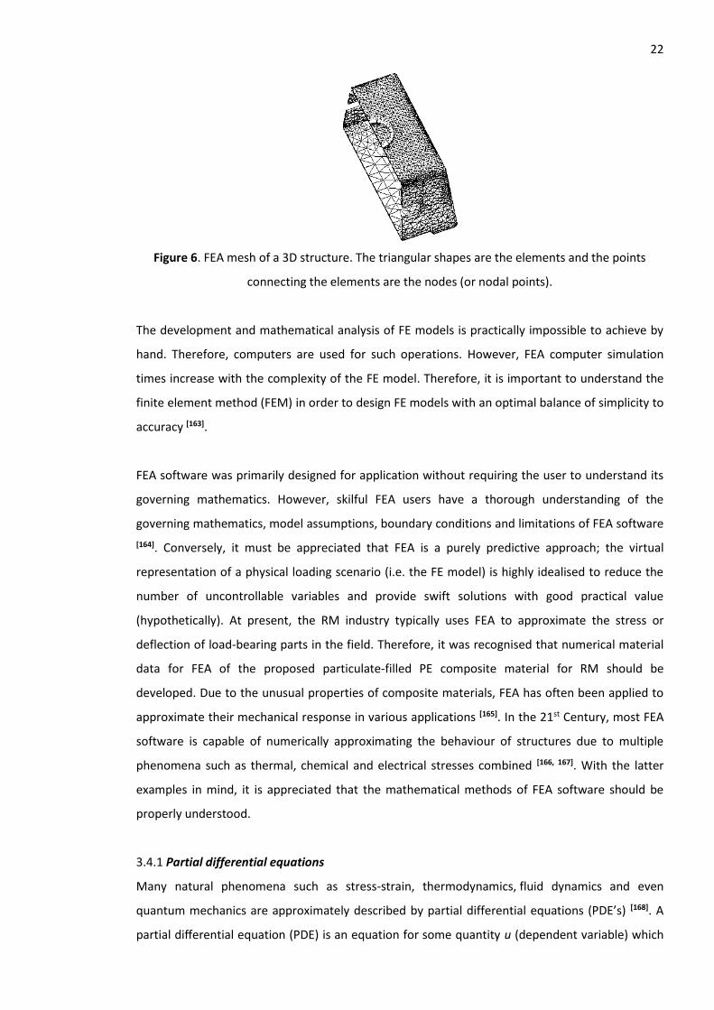
connected by lines to form a mesh of simple shapes (e.g. tetrahedrons, called finite elements)

around a 2D or 3D structure [161] (Figure 6). The solutions of PDE’s are functions assigned to the

nodes forming the finite elements [162]. Stress or strain is calculated at the nodes and then an

approximation across the entire mesh of elements is provided (under the given equilibrium and

loading conditions).

22

Figure 6. FEA mesh of a 3D structure. The triangular shapes are the elements and the points

connecting the elements are the nodes (or nodal points).

The development and mathematical analysis of FE models is practically impossible to achieve by

hand. Therefore, computers are used for such operations. However, FEA computer simulation

times increase with the complexity of the FE model. Therefore, it is important to understand the

finite element method (FEM) in order to design FE models with an optimal balance of simplicity to

accuracy [163].

FEA software was primarily designed for application without requiring the user to understand its

governing mathematics. However, skilful FEA users have a thorough understanding of the

governing mathematics, model assumptions, boundary conditions and limitations of FEA software

[164]. Conversely, it must be appreciated that FEA is a purely predictive approach; the virtual

representation of a physical loading scenario (i.e. the FE model) is highly idealised to reduce the

number of uncontrollable variables and provide swift solutions with good practical value

(hypothetically). At present, the RM industry typically uses FEA to approximate the stress or

deflection of load-bearing parts in the field. Therefore, it was recognised that numerical material

data for FEA of the proposed particulate-filled PE composite material for RM should be

developed. Due to the unusual properties of composite materials, FEA has often been applied to

approximate their mechanical response in various applications [165]. In the 21st Century, most FEA

software is capable of numerically approximating the behaviour of structures due to multiple

phenomena such as thermal, chemical and electrical stresses combined [166, 167]. With the latter

examples in mind, it is appreciated that the mathematical methods of FEA software should be

properly understood.

3.4.1 Partial differential equations

Many natural phenomena such as stress-strain, thermodynamics, fluid dynamics and even

quantum mechanics are approximately described by partial differential equations (PDE’s) [168]. A

partial differential equation (PDE) is an equation for some quantity u (dependent variable) which

23 is a function of the independent variables x1, x2, x3 … xn (provided n ≥ 2) and involves derivatives of

u with respect to at least some of the independent variables [169]. Ordinary differential equations

describe one-dimensional dynamic systems whereas partial differential equations can

describe multi-dimensional systems; PDE’s contain unknown multi-variable functions and

their partial derivatives, relative to ordinary differential equations which contain single variable

functions and their derivatives [170]. PDE’s may be solved by hand (impractical for complex

problems) or ordered to create a relevant computer model (e.g. a FE model). Various sets of PDE’s

have been developed to approximate natural phenomena such as the Helmholtz equation, Klein-

Gordon equation and Poisson's equation.

PDE’s may be solved analytically or numerically. Analytical solutions are closed form as the

solution can be described as a single mathematical function [171]. The analytical solution is easily

achievable for very simple problems and becomes impractical to obtain for complex PDE’s with a

large number of independent variables. In the ideal world, analytical solutions would arguably be

the preferred choice as it provides a single mathematical function that describes the systems

behaviour at any given instance. However, analytical solutions are usually difficult to understand

or impractical to develop for complex problems which involve multiple variables. Numerical

solutions use a numerical time-stepping procedure to provide a basic solution at any given time in

the form of time-stepping graph, allowing observation of the change in variables with respect to

time [172]. Numerical solutions approximate as close as possible to the analytical solution with

respect to these time-steps. Therefore, the accuracy of the final solution is dependent upon the

size of the time steps i.e. smaller time steps will give a solution more closely linked to the

analytical solution. However, many iterative calculations are required for better accuracy; as the

time steps decrease, the number of iterative calculations increases. The latter condition highlights

the trade-off between time and accuracy for numerical and analytical solutions. However, modern

advances in computing speed have greatly leaped the practicality of solving PDE’s numerically.

Currently, there are various numerical methods used to solve PDE’s such as the finite volume

method (FVM), the finite difference method (FDM) and the finite element method (FEM). For the

purpose of this study, the FEM has been selected for further discussion.

3.4.2 History of the finite element method

Although the development of methods to solve PDE’s can arguably be traced back as far as the

late 16th Century [173], a paper by Courant et al. in 1928 [174] detailed the considerations for time-

dependent PDE solutions. Furthermore, in 1943 R. Courant utilised the Rayleigh-Ritz method of

minimisation of variational calculus and numerical analysis to deduce approximate solutions for

vibrational systems [175, 176]. Prager and Synge used triangular elements to solve a 2D elasticity

24 problem using the hypercircle method in 1947 [177]. The works by R. Courant et al. were extremely

influential on the first FEA computer software developed by the European and American aircraft

industries in the 1950’s, using expensive, large mainframe computers [178]. However, in 1955

Argyris published work on energy methods in structural analysis, thus creating the force method

of FEA [179]. Moreover, in 1956 a paper on the stiffness and deflection of complex structures by M.

J. Turner et al. [180] established a wider definition of numerical analysis for PDE’s. R.W. Clough first

used the term “Finite Element Method” in 1960 [181]. By the early 1970’s, FEA was limited to

expensive mainframe type computers only available to heavy industries such as automotive,

aerospace, defence and even nuclear. However, the introduction of personal computers in the

1980’s provided wider access to FEA software from numerous vendors.

3.4.3 Theory and Requirements of the Finite Element Method

The underlying theory of FEA is a selection of discrete PDE’s defined at nodes that form a mesh of

elements across a geometry. FEA software reduces the PDE’s governing the underlying physics of

the model into a series of trial functions to be evaluated at nodal points defined by the mesh [182].

The result is an approximation of stress, strain or displacement, at any nodal point or element or

across the structure. Such an interpretation is a wide generalisation. However, it is highly flexible

in terms of application and can have good practical value. In order to highlight the theory of FEA,

a generalised solution for static linear-elastic isotropic problems is discussed in this section.

Generally, it is common to determine the structural behaviour of a body that is in static

equilibrium, indicating that the sum of all forces acting on the body equal zero. Therefore, in

order to conduct FEA the following pre-requisites must be met [183]:

The material properties are known e.g. the tensile modulus, yield stress and Poisson’s

ratio

The geometry of the body in its unloaded state is fully defined (R). The latter is usually

imported into the software in the form of a CAD file.

The elastic constants (𝐶𝑖𝑗𝑘𝑙) of the solid are known.

The boundary conditions i.e. the magnitude and distribution of the force (𝑏) and/or

displacements (u*(x)) on a portion (δ1R) of the body in its unloaded state are accurately

defined.

The latter pre-requisites are sufficient if thermal effects acting on the body are negligible, the

material is isotropic, the displacements are relatively small and there is no contact with other

bodies. The FEM begins by summarising the following governing equations of the model to solve

for the displacement field (𝑢𝑖𝑗), stress field (𝜎𝑖𝑗 ) and strain field (휀𝑖𝑗):

25

The strain-displacement equation [184] → 휀𝑖𝑗 =1

2(

𝜕𝑢𝑖

𝜕𝑥𝑗+

𝜕𝑢𝑗

𝜕𝑥𝑖) Equation 3.

The elastic stress-strain law [185] → 𝜎𝑖𝑗 = 𝐶𝑖𝑗𝑘𝑙휀𝑘𝑙 Equation 4.

The static equilibrium of stresses equation [186] → 𝜕𝜎𝑖𝑗

𝜕𝑥𝑖+ 𝑏𝑗 = 0 Equation 5.

The boundary conditions on displacement → 𝑢𝑖𝑗 = 𝑢𝑖𝑗∗ on δ1R Equation 6.

PDE’s 3 and 5 are generally solved using the principle of virtual work [187]; this re-defines the

equations in integral form for easier manipulation. The main objective of the FEM is to calculate

the displacement within a body subjected to external forces; if one were to visualise a solid body

undergoing deformation due to external load, a suitably defined point on the body will move with

the application of the load. The displacement vector (u*(x)) will define the motion of this point at

position x in the undeformed body. Once u*(x) has been determined, the distribution and

magnitude of stress-strain fields across the entire body can be deduced.

3.4.4 Finite element model development

FEA may be conducted in three stages respectively; FE model development, analysis and

refinement. Due to the wealth of options within FEA software, only a selection of analysis types,

model refinement techniques and material properties used for investigations within this thesis

are elaborated upon. Primarily, two types of analyses can be conducted within FEA software;

static linear-elastic and non-linear. Static linear-elastic analyses are suitable for many simple to

intermediate engineering problems. However, static linear-elastic simulations are highly idealised

rendering them unsuitable for more complex scenarios. For example, the static term describing

linear-elastic simulations indicates the entire load is applied at one instance. Therefore, a static

linear-elastic analysis would not be suitable for vibratory or sinusoidal loading scenarios.

Non-linear analyses are more suitable when excessively large stresses/strains (beyond the yield

stress of the material) and complex loading scenarios are anticipated. However, designing non-

linear FE models requires significantly more time, information and careful representation of the

loading scenario relative to static linear-elastic simulations. Furthermore, when designing non-

linear FE models it is crucial to avoid the complexity of the model reaching the complexity of the

problem in the physical world. To reduce simulation times, numerical elimination methods (such

as Gaussian elimination) may be used for the analysis of FE models with thousands of functions.

However, when the amount of calculations reaches several million, the non-linear solutions

become too expensive in terms of time and computing memory. In such circumstances special

iterative methods such as the Newton-Raphson method are used, although the solution time of

these methods depends on the required accuracy [188]. Overall, it is clear that identifying a suitable

26 balance between FE model simplification and accuracy is critical for reducing simulation times, a

judgement made better by skilful users who have a thorough understanding of the methods,

boundary conditions and limitations of FEA.

3.4.4.1 Static linear-elastic analyses

Static linear-elastic FEA offers quick solution times at the expense of highly idealising the model;

in essence, such models assume the structure and material to obey Hooke’s Law, whereby the

stress-strain response of the material is linear and the structure returns to its original state upon

removal of the load [189]. The tensile modulus of a material is the gradient of its tensile stress-

strain response up to the yield point. Beyond the yield point is the onset of non-linearity.

Therefore, static linear-elastic simulations are suitable when stresses below the yield point of the

material are anticipated. Generally, engineering designs require a high factor of safety to ensure

that the stresses operate well below the yield point of the material. Therefore, static-linear elastic

simulations are common procedure for FEA. Consequently, the matrix function describing the

static linear-elastic assumption is:

{𝐹} = [𝐾]{𝑢} Equation 7.

Where:

{K} = Global stiffness matrix of the structure

{F} = External force matrix

{u} = Displacement matrix

In order for the static linear-elastic assumption to be valid, the loads must be constant in

magnitude and distribution [190], the applied stress should be lower than the yield stress of the

material and the boundary conditions should remain constant from the instance of loading to the

final deformed shape. Furthermore, static linear-elastic analysis assumes the entire load is applied

at one instance and the stiffness of the structure is independent of any load or displacement [191];

a geometric stiffening phenomenon can occur when a structure is loaded resulting in decreased

displacement with increased load, such factors are not fully accounted for in static linear-elastic

FE models. However, the static linear-elastic assumption may be used in circumstances where

steady state and constant magnitude are observed; for example, the structural response of a body

travelling at a constant velocity or acceleration can be modelled as static. The static assumption

loses its validity when, for example, the structure’s stiffness causes the load to be removed before

the full response can be gauged or when the load excites vibrations within the structure.

Technically speaking, a static linear-elastic situation seldom exists in the physical world. However,

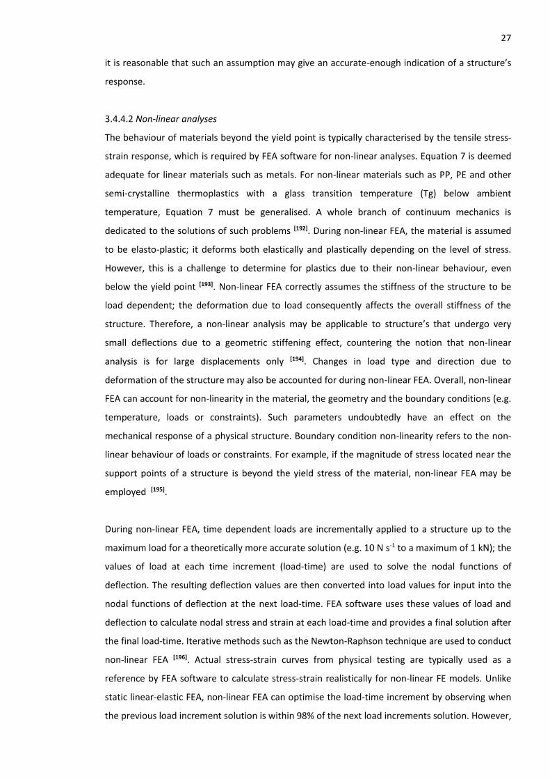
27 it is reasonable that such an assumption may give an accurate-enough indication of a structure’s

response.

3.4.4.2 Non-linear analyses

The behaviour of materials beyond the yield point is typically characterised by the tensile stress-

strain response, which is required by FEA software for non-linear analyses. Equation 7 is deemed

adequate for linear materials such as metals. For non-linear materials such as PP, PE and other

semi-crystalline thermoplastics with a glass transition temperature (Tg) below ambient

temperature, Equation 7 must be generalised. A whole branch of continuum mechanics is

dedicated to the solutions of such problems [192]. During non-linear FEA, the material is assumed

to be elasto-plastic; it deforms both elastically and plastically depending on the level of stress.

However, this is a challenge to determine for plastics due to their non-linear behaviour, even

below the yield point [193]. Non-linear FEA correctly assumes the stiffness of the structure to be

load dependent; the deformation due to load consequently affects the overall stiffness of the

structure. Therefore, a non-linear analysis may be applicable to structure’s that undergo very

small deflections due to a geometric stiffening effect, countering the notion that non-linear

analysis is for large displacements only [194]. Changes in load type and direction due to

deformation of the structure may also be accounted for during non-linear FEA. Overall, non-linear

FEA can account for non-linearity in the material, the geometry and the boundary conditions (e.g.

temperature, loads or constraints). Such parameters undoubtedly have an effect on the

mechanical response of a physical structure. Boundary condition non-linearity refers to the non-

linear behaviour of loads or constraints. For example, if the magnitude of stress located near the

support points of a structure is beyond the yield stress of the material, non-linear FEA may be

employed [195].

During non-linear FEA, time dependent loads are incrementally applied to a structure up to the

maximum load for a theoretically more accurate solution (e.g. 10 N s-1 to a maximum of 1 kN); the

values of load at each time increment (load-time) are used to solve the nodal functions of

deflection. The resulting deflection values are then converted into load values for input into the

nodal functions of deflection at the next load-time. FEA software uses these values of load and

deflection to calculate nodal stress and strain at each load-time and provides a final solution after

the final load-time. Iterative methods such as the Newton-Raphson technique are used to conduct

non-linear FEA [196]. Actual stress-strain curves from physical testing are typically used as a

reference by FEA software to calculate stress-strain realistically for non-linear FE models. Unlike

static linear-elastic FEA, non-linear FEA can optimise the load-time increment by observing when

the previous load increment solution is within 98% of the next load increments solution. However,

28 this may be user specified. The latter process is known as solution convergence. Therefore, the

timing of the load increment should be sufficiently optimised to observe solution convergence

[197].

3.4.5 Finite element model refinement

The fundamental purpose of FE model refinement is to increase mesh quality to reduce

experimental error. FEA software calculates stress and strain at nodal points defining the mesh.

Therefore, it is crucial that the mesh is properly defined. Determining the exact number, size and

shape of elements to optimise a FE model is not possible. Moreover, refining a mesh to ensure

low approximation errors and avoid long solution times simultaneously can be a difficult and

time-consuming task [198]. However, the application of mesh refinement is certainly individual to

the boundary conditions of model. Therefore, the importance of a good mesh for FEA cannot be

overemphasized [199]. Conversely, over-refining the mesh may increase simulation time

considerably for little gain in accuracy. To simplify the refinement process, the mesh can be

iteratively refined until the solution of the model converges to a user specified limit e.g. the

elemental solutions of stress or strain are within 98 % of the equivalent nodal solutions, the latter

is called relative strain error convergence. Other common convergence options for FEA are:

Strain energy convergence - The strain energy of the model is calculated by summing the

strain energy of the elements. Strain energy convergence is a better criterion for

optimizing an FEA mesh; the average strain energy of the elements is influenced by mesh

size and elemental order, rather than structural geometry.

Stress convergence – Convergence occurs when the solutions of stress reach a limiting

value. Convergence is difficult to achieve with this method if stress concentration points

are observed. The concentrated stress simply increases with the increase in mesh density.

Some degree of mesh coarsening (reduction of nodal points) at points of stress

concentration can reduce this effect.

Deflection convergence - nodal deflection values are used for the convergence criterion.

Mesh refinement may be automated (known as adaptive meshing) or manually conducted by

skilful users [200]. Adaptive mesh refinement usually increases the number of elements in areas of

interest by decreasing their size. A FE mesh is characterized by the local mesh size “H”, the

element order “P” and the nodal positions “R” for the solutions of stress or deflection across the

mesh [201]. The H and P mesh refinement methods are extensively implemented within FEA

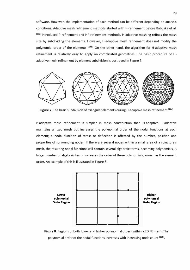
29 software. However, the implementation of each method can be different depending on analysis

conditions. Adaptive mesh refinement methods started with H-refinement before Babuska et al.

[202] introduced P-refinement and HP-refinement methods. H-adaptive meshing refines the mesh

size by subdividing the elements. However, H-adaptive mesh refinement does not modify the

polynomial order of the elements [203]. On the other hand, the algorithm for H-adaptive mesh

refinement is relatively easy to apply on complicated geometries. The basic procedure of H-

adaptive mesh refinement by element subdivision is portrayed in Figure 7.

Figure 7. The basic subdivision of triangular elements during H-adaptive mesh refinement [204]

P-adaptive mesh refinement is simpler in mesh construction than H-adaptive. P-adaptive

maintains a fixed mesh but increases the polynomial order of the nodal functions at each

element; a nodal function of stress or deflection is affected by the number, position and

properties of surrounding nodes. If there are several nodes within a small area of a structure’s

mesh, the resulting nodal functions will contain several algebraic terms, becoming polynomials. A

larger number of algebraic terms increases the order of these polynomials, known as the element

order. An example of this is illustrated in Figure 8.

Figure 8. Regions of both lower and higher polynomial orders within a 2D FE mesh. The

polynomial order of the nodal functions increases with increasing node count [205].

30 P-adaptive mesh refinement is particularly useful for complex elements that deform due to both

compression and tension [206]. The HP-adaptive mesh refinement type combines the approach of

both H and P-adaptive meshing [207]. R-adaptive mesh refinement maintains the number of nodes

in the original mesh. However, the positions of these nodes are relocated to where better

resolution is required [208].All three methods (H, P and R-adaptive) have individually achieved

success in FEA studies [209, 210, 211]. However, the consideration of all three adaptive mesh

refinement methods (H, P and R) should be made during FEA. The accuracy of FEA is heavily

dependent on the mesh size selected; a smaller mesh size can minimise the error incurred by

extrapolating data between nodes. On the other hand, a fine mesh increases the computational

cost of the analysis in terms of simulation time. Therefore, a skilful FEA user should have

adequate experience and knowledge with each mesh refinement method to understand its

application. To conclude, the following steps summarise the basic procedure of FEA software:

1. A 2D or 3D structure is graphically divided into small elements (sections or regions of

shape).

2. A mechanical stress-strain response is defined at the elements by a set of PDE’s. The

PDE’s are converted into polynomial functions suitable for a computer-aided solution.

3. The element functions are combined and a global structural function is obtained.

4. The load and boundary conditions are then incorporated in the global function

5. The individual functions are solved and a deflection for each node is calculated.

6. The deflection values are then inserted into the global function to solve for overall stress

and strain of the structure.

7. Refinements are made to the original model, if necessary.

3.5 Finite Element Analysis of Rotomoulded Parts

In the context of RM, little published research regarding FEA is available [23]; the FEA of

rotomoulded parts often remains confidential in the RM industry, creating an environment that

promotes the retention (rather than the dissemination) of vital experience and data with regards

to FEA. The RM industry mostly outsources FEA to external consultancies, understandably due to

their own lack of expertise in using such software. Furthermore, if any preliminary design

revisions resulting from FEA were made, rotomoulders can defend claims of negligence if a part

fails in the field [212]. It is apparent that the accuracy of FEA software is dependent on the

credibility of input data (material properties, geometry and load scenario). Parameters such as

geometrical dimensions, material properties and model assumptions play an important role in the

accuracy of FEA. With this in mind, it is appreciated that the geometry of rotomoulded products

vary significantly relative to injection moulded products, due to the absence of applied pressure.

31 Therefore, conducting FEA on large rotomoulded products (such as underground water tanks

where wall thicknesses can exceed 50 mm) presents a formidable challenge to engineers due to

substantial differences between the FE model and the physical rotomoulded product. These

differences are:

The variation in wall thickness.

The complex non-linear behaviour of PE at low strains.

The lack of experimental data regarding the compressive behaviour and Poisson’s ratio of

PE.

Such factors are not entirely considered during the FEA of rotomoulded parts, leading to instances

of unexpected behaviour in the field. Therefore, identifying the critical factors affecting the use of

FEA for rotomoulded parts is explored within this thesis, in order to develop an inclusive FE

modelling procedure. Consequently, the extensive use of FEA in the modern engineering world

exemplifies the importance of developing a numerical material property database for the

proposed new particulate-filled PE composite materials. The latter materials should instil

confidence in rotomoulders who are expected to use them via accurate FEA approximations of

their performance. Combining physical test data from rotomoulded parts with FEA was the

selected approach; a venture seemingly unheeded in the RM industry today. Data from the

material specification sheets of PE suppliers are often inappropriate for FEA and vary

considerably. A common example of this is the tensile modulus of PE; due to the non-linearity of

PE’s stress-strain response, the tensile modulus is an over-estimation of its true capability. A high

modulus composite material accompanied by accurate numerical material property data for FEA

could expand the current application envelope for RM. The latter formed the rationale behind the

composite development and FEA investigations in this thesis.

3.6 Summary of Literature Review

To conclude, the following points of interest from the literature review are summarised:

RM has progressed considerably (and is continuing to progress) from a relatively primitive

technique to a method highly regarded by manufacturers for complex, load bearing

structures.

PE is the most common material used in modern day RM products because of its cheap

cost, good toughness and suitable melt flow properties, relative to alternative polymer

32

grades. However, the stiffness limitation of PE narrows the application envelope for

manufacturers.

Fillers have been known to reduce the cost of polymer products. However, this effect is

generally superseded by the reinforcing effects. Filler characteristics such as shape, size,

elemental composition and aspect ratio play significant roles in determining the

effectiveness of particulate-fillers as reinforcements for polymers.

Optimisation of particulate-filled polymers is only possible when the filler particles have

been treated with chemical agents to increase the strength of adhesion between the

polymer matrix and the filler particle (filler-matrix interaction) and disperse the particles

evenly. The latter additives are known as coupling agents and dispersion agents

respectively.

PE is well known to have low polarity (chemically stable). Therefore, it is somewhat

tedious to find a coupling agent to functionalise the PE matrix for better compatibility

with the filler particle surfaces; this can increase matrix-filler interaction and thus increase

the mechanical performance of the resulting composite.

RM is a zero-shear process (unlike many conventional plastics moulding processes such as

injection or blow moulding). The lack of pressure induced flow of the polymer melt

challenges particulate-filled polymer composite materials; the melt flow properties of the

resulting composites are often reduced.

Computer aided engineering (CAE) technologies such as computer aided design (CAD) and

finite element analysis (FEA) offer the capability to build, optimise and validate

engineering designs within a virtual environment.

In the context of RM, manufacturers and their clientele use CAE softwares such as FEA

and CAD to estimate whether load-bearing parts will be within the overall dimensions

specified, withstand the loads required and endure the intended lifecycle.

FEA is ultimately a numerical approximation for solving boundary value and solid

mechanics problems. It is the most extensively used numerical analysis method in

mechanical engineering practice. The mechanical response of structures can be analysed

using FEA software with relative ease.

33

The fundamental concept of FEA is the assumption that any continuous quantity such as

stress or deflection can be numerically approximated by a discrete mathematical model

composed of iterative partial differential equations (PDE’s).

FEA software was first developed in the 1950’s. By the early 1970’s, FEA was limited to

expensive mainframe type computers only available to heavy industries such as

automotive, aerospace, defence and nuclear. However, the introduction of personal

computers in the 1980’s provided access to FEA software from numerous vendors.

Primarily, two types of analyses can be conducted using FEA software; static linear-elastic

and non-linear. Static linear-elastic analyses are suitable for many simple to intermediate

engineering problems. However, static linear-elastic analyses are highly idealised for

quicker solution times rendering them unsuitable for more complex scenarios.

Non-linear FEA is more suitable when large stresses/strains (beyond the yield stress of the

material) and complex loading scenarios are anticipated. However, designing non-linear

FE models requires significantly more time, information and careful representation of the

loading scenario. Overall, non-linear simulations can account for non-linearity in the

material, the geometry and the boundary conditions.

Identifying a suitable balance between simplification and accuracy in order to reduce

simulation times is crucial; a judgement made better by skilful FEA users who have a

thorough understanding of analysis methods, boundary conditions and limitations.

The fundamental purpose of FE model refinement is to increase mesh quality to reduce

experimental error. The accuracy of FEA is heavily dependent on the mesh size selected; a

smaller mesh size can minimise the error incurred by extrapolating data between nodes.

On the other hand, a finer mesh increases the cost of the analysis in terms of time and

computer operating speed.

Adaptive mesh refinement usually increases the number of elements in areas of interest

by decreasing the size of elements. A FE mesh is characterized by the local mesh size “H”,

the element order “P” and the nodal positions “R”.

H-adaptive mesh refinement subdivides elements but maintains the order of the element.

Moreover, the algorithm for H-refinement is easy to apply to complicated geometries. P-

34

adaptive mesh refinement is simpler in mesh construction than H-adaptive. P-adaptive

maintains a fixed mesh but increases the polynomial order of the nodal functions at each

element.

In the context of RM, little published research regarding FEA is available. The RM industry

mostly outsources FEA to external consultancies, understandably due to their own lack of

expertise using such techniques.

The FEA of large rotomoulded products presents a formidable challenge to engineers due

to substantial differences between the FE model and the physical rotomoulded product,

such as wall thickness variation and the non-linear behaviour of PE.

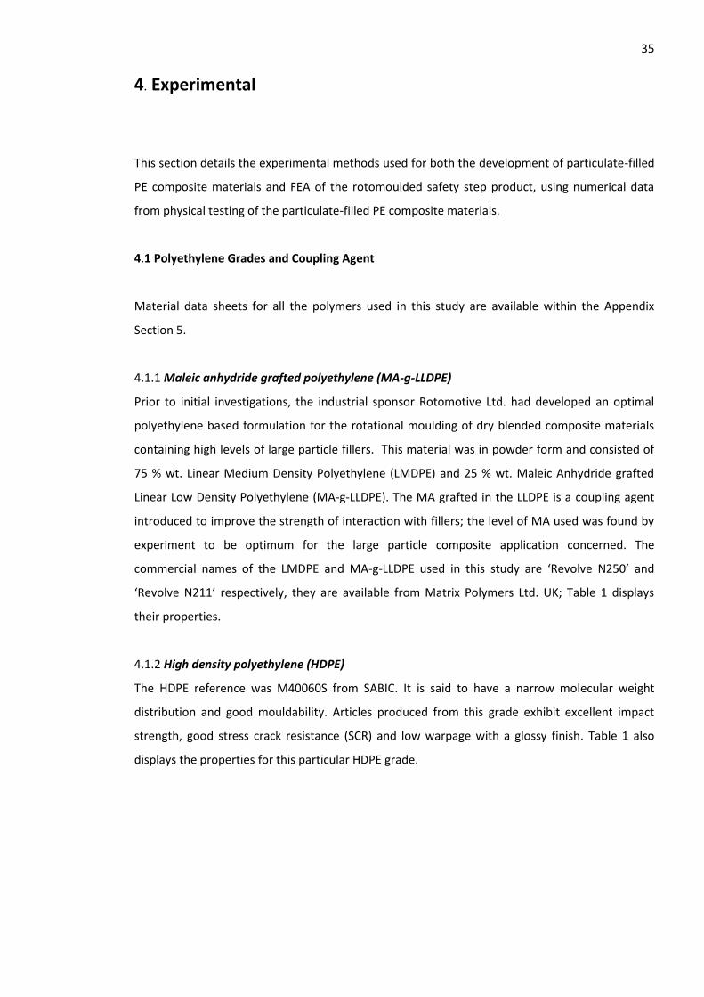
35

4. Experimental

This section details the experimental methods used for both the development of particulate-filled

PE composite materials and FEA of the rotomoulded safety step product, using numerical data

from physical testing of the particulate-filled PE composite materials.

4.1 Polyethylene Grades and Coupling Agent

Material data sheets for all the polymers used in this study are available within the Appendix

Section 5.

4.1.1 Maleic anhydride grafted polyethylene (MA-g-LLDPE)

Prior to initial investigations, the industrial sponsor Rotomotive Ltd. had developed an optimal

polyethylene based formulation for the rotational moulding of dry blended composite materials

containing high levels of large particle fillers. This material was in powder form and consisted of

75 % wt. Linear Medium Density Polyethylene (LMDPE) and 25 % wt. Maleic Anhydride grafted

Linear Low Density Polyethylene (MA-g-LLDPE). The MA grafted in the LLDPE is a coupling agent

introduced to improve the strength of interaction with fillers; the level of MA used was found by

experiment to be optimum for the large particle composite application concerned. The

commercial names of the LMDPE and MA-g-LLDPE used in this study are ‘Revolve N250’ and

‘Revolve N211’ respectively, they are available from Matrix Polymers Ltd. UK; Table 1 displays

their properties.

4.1.2 High density polyethylene (HDPE)

The HDPE reference was M40060S from SABIC. It is said to have a narrow molecular weight

distribution and good mouldability. Articles produced from this grade exhibit excellent impact

strength, good stress crack resistance (SCR) and low warpage with a glossy finish. Table 1 also

displays the properties for this particular HDPE grade.

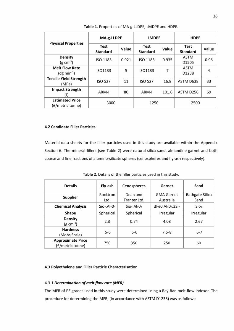
36

Table 1. Properties of MA-g-LLDPE, LMDPE and HDPE.

Physical Properties MA-g-LLDPE LMDPE HDPE

Test Standard

Value Test

Standard Value

Test Standard

Value

Density (g cm-3)

ISO 1183 0.921 ISO 1183 0.935 ASTM D1505

0.96

Melt Flow Rate (dg min-1)

ISO1133 5 ISO1133 7 ASTM D1238

4

Tensile Yield Strength (MPa)

ISO 527 11 ISO 527 16.8 ASTM D638 33

Impact Strength (J)

ARM-I 80 ARM-I 101.6 ASTM D256 69

Estimated Price (£/metric tonne)

3000 1250 2500

4.2 Candidate Filler Particles

Material data sheets for the filler particles used in this study are available within the Appendix

Section 6. The mineral fillers (see Table 2) were natural silica sand, almandine garnet and both

coarse and fine fractions of alumino-silicate spheres (cenospheres and fly-ash respectively).

Table 2. Details of the filler particles used in this study.

Details Fly-ash Cenospheres Garnet Sand

Supplier Rocktron

Ltd. Dean and

Tranter Ltd. GMA Garnet

Australia Bathgate Silica

Sand

Chemical Analysis Sio2.Al203 Sio2.Al203 3Fe0.Al203.3Si2 Sio2

Shape Spherical Spherical Irregular Irregular

Density (g cm-3)

2.3 0.74 4.08 2.67

Hardness (Mohs Scale)

5-6 5-6 7.5-8 6-7

Approximate Price (£/metric tonne)

750 350 250 60

4.3 Polyethylene and Filler Particle Characterisation

4.3.1 Determination of melt flow rate (MFR)

The MFR of PE grades used in this study were determined using a Ray-Ran melt flow indexer. The

procedure for determining the MFR, (in accordance with ASTM D1238) was as follows:

37

1. A small amount of PE (ca. 4-5 g weighed on a Sartorius model AC 120 S four figure

balance) was placed into the extruder barrel of the Ray Ran MFR apparatus. At the end of

the extrudate barrel is a small die of approximately 2mm in diameter.

2. The PE was compressed into the extruder barrel (using a metal plunger) in 0.5 g intervals

to avoid the formation of air bubbles.

3. The sample was then preheated for 5 min at approximately 190 °C.

4. A 2.16 kg piston was then placed into the barrel (on top of the PE) to introduce the shear

force required to extrude the PE through the die at the output end of the barrel.

5. A sample of the melt was then taken after a period of ten minutes and weighed to give

the resulting MFR (expressed as g/10 minutes or dg min-1 ).

6. Each determination was replicated four times and an average value reported.

4.3.2 Estimation of filler particle maximum packing fraction (MPF)

MPF tests (essentially oil absorption tests) were carried out in order to estimate the maximum

amount of filler that can be incorporated into a PE matrix. Rather than linseed oil (as would be

used in a conventional oil absorption test), liquid paraffin was used as the liquid medium. Liquid

paraffin is chemically very similar to PE; in fact the basic structure (mixed alkanes) is identical to

PE, the alkyl chains in liquid paraffin are however much shorter. Linseed oil (mainly linolenic acid)

is more polar than PE and could therefore give unsuitable data. The test involved placing a known

mass of filler (ca. 1 g weighed on a Sartorius Model AC 120 S four figure balance) on to a clean

white tile. Liquid paraffin was added drop-wise to the pile of filler from a burette. A palette knife

was used to mix the filler and liquid paraffin mixture, making sure that it was spread into a neat

pile. Just enough liquid paraffin was added to fully wet out the powder particles such that a

homogeneous putty-like mass was formed whilst mixing with the spatula. The latter change in

property forms a surprisingly well defined end point. Reproducibility was typically ± 0.01 % vol.

Each determination was replicated three times and the average titre reported. The maximum

packing fraction (MPF) was then calculated by volume and mass, using Equations 8 and 9

respectively. Equation 8 was used to convert mass into volume and vice versa, for input into

Equations 9 and 10.

𝜌 =𝑚

𝑣 Equation 8.

Where:

m = Mass of powdered material (g)

v = Volumetric displacement of water (ml)

𝜌 = Density of material (g cm-3)

38

𝑉𝑝𝑓 = 𝑉𝑓

𝑉𝑓+𝑉𝑙 Equation 9.

Where:

Vpf = Maximum packing fraction volume (between 0 and 1)

vf =Volume of filler (cm3)

vl = volume of liquid paraffin (cm3)

𝑀𝑝𝑓 = 𝑀𝑓

𝑀𝑓+𝑀𝑙 Equation 10.

Where:

Mpf = Maximum packing fraction by mass (between o and 1)

ml= Mass of liquid paraffin (g)

mf = Mass of filler (g)

4.3.3 Determination of filler particle densities

4.3.3.1 Sand, garnet and fly-ash

The densities of sand, garnet and fly-ash were calculated directly by slowly sprinkling a pre-

determined mass (ca. 200 g weighed on a Mettler model PE11 one figure balance) of each

material into a measuring cylinder containing water to measure the resulting volumetric

displacement. The corresponding values of mass and volume were then used to calculate the

density using Equation 8. Three repeat tests were conducted and the average density and

standard deviation was calculated. Candidate fillers used in this work were not porous, this is

apparent in scanning electron microscope (SEM) images of the filler particles (Results and

Discussion Section 5.3.1, Figures 44-48) where the filler particles have a solid non-porous surface.

Fly-ash and cenosphere particles are essentially hollow spheres filled with air.

4.3.3.2 Cenospheres

Cenospheres float on water due to their low density relative to water. Therefore, a liquid of lower

density than water was used for cenosphere density tests; petroleum ether (60-88 °C boiling

range, density 0.67 g cm-3). Prior to conducting the test, a jar and lid were weighed using a

Mettler model PE11 one figure balance. The jar was then totally filled with petroleum ether,

sealed with the lid (to prevent the petroleum ether from evaporating) and the total mass of the

jar, lid and petroleum ether was recorded. Next the jar was emptied, rinsed thoroughly and dried

before repeating the same process again with the addition of cenospheres. The mass of

petroleum ether in the jar (both with and without cenospheres) was deduced and converted to

volume using Equation 8. The difference between the two measured volumes (as a result of

39 cenosphere addition) was then calculated; the resulting volume and known mass of cenospheres

were then used to calculate the density, using Equation 8. Three repeat tests were conducted and

the average density and standard deviation was calculated.

4.3.4 Verification of filler particle size distribution

Sieve analyses on the large particle fillers were conducted using a Rotap shaker, test sieves and

pan. The latter equipment is a vertical stack of sieves, whereby the top sieve is of a larger size

than the sieve underneath. For this investigation, the sieve sizes (in descending order from the

top) were 500, 425, 300, 212, 150 and 90 µm, leading to a pan at the very bottom to collect

remaining particles. The shaker is used to ensure the filler particles are effectively drawn through

the sieves. The test procedure was as follows:

Sieves were arranged in the order specified and a 100 g sample was placed into the top

sieve.

A lid was placed on the top sieve and secured to the Rotap sieve shaker.

A 10 minute timer was set on the control pad of the sieve shaker and the start button was

pressed via the analogue control panel.

After 10 minutes, the top sieve was placed on the scale and the tare was set to zero.

The sieve was then removed, any remaining material was cleaned and the new weight of

the sieve was then recorded.

This process was then repeated with all the remaining sieve sizes. The weights were

totalled and recorded.

4.3.5 Determination of PE/filler composite densities

4.3.5.1 Densometer method

Composite PE/filler density was determined using an Ohaus Voyager Pro densometer. The

densometer has a combined weighing scale and jug facility which allows the user to weigh a solid

material in air and water, both of which the densometer records. The densometer then uses

Archimedes principle to calculate the density, utilising the values of apparent weight in air and

apparent weight in water using Equation 11.

40

𝜌𝑚

𝜌𝑤=

𝑚

𝑚−𝑚𝑤 Equation 11.

Where:

𝜌m= Density of material (g cm-3)

𝜌w= Density of water (g cm-3)

m = Mass of material in air (g)

mw= Apparent mass of material in water (g)

4.3.5.2 Ashing method

Ashing to determine the density of melt compounded PE/fly-ash composites was conducted using

a Carbolite electric oven, a glass desiccator containing silica gel beads (to absorb moisture) and

ceramic crucibles. The desiccator had a valve on the lid for air pressure relief. A thin layer of

petroleum jelly was applied by hand on the surface of the lid and desiccator to create an airtight

seal. The following test procedure was applied:

1. The crucibles were treated in the oven for 2 hours at 860 oC to burn off any organic

residues.

2. The PE/fly-ash composite samples and crucibles were weighed using a Sartorius Model AC

120 S four figure balance.

3. One crucible was filled with fly-ash and the other crucibles were filled with the PE/fly-ash

composite samples.

4. All crucibles were placed in the desiccator, sealed air-tight and placed in the oven at

100oC for two hours to remove any moisture.

5. The crucibles and their contents were weighed and placed back into the oven at 800 oC

for two hours to burn off the PE in the PE/fly-ash materials.

6. The remaining filler content in the crucibles were weighed. Equations 12, 13 and 14 were

used to calculate composite filler content and ultimately total composite density (using

Equation 15).

𝐹𝑟 = 𝑚𝑓/𝑚𝑓𝑑 Equation 12.

Where:

Fr = Residue fraction of fly-ash after 800 oC

mf = Mass of fly-ash (g)

mfd = Mass of fly-ash after the 100o C drying period (g)

41

𝑀𝑓𝑐 = 𝑚𝑐𝑟/𝑓𝑟 Equation 13.

Where:

Mfc = Mass of fly-ash in composite (g)

mcr = Mass residue of composite after 800 oC period (g)

fr = Residue fraction of fly-ash

𝐹𝑐 =𝑚𝑓𝑐

𝑚𝑓𝑑× 100 Equation 14.

Where:

Fc = Fly-ash content (% wt.)

mfc = Mass of fly-ash in composite (g)

mfd = Mass of composite after the 100 oC drying period (g)

𝜌𝑇 =1

(𝑚𝑓 𝜌𝑓⁄ )+((1−𝑚𝑓) 𝜌𝑝⁄ ) Equation 15.

Where:

ρT = Total composite density

mf = Mass of filler material (g)

ρf = Density of filler (g cm-3)

ρp = Density of polymer (g cm-3)

4.4 Blending of Filler Particles and Polyethylene to Form Composite Materials

4.4.1 Dry blended formulations

Composites were prepared by pre-mixing the filler and PE in the bowl of a planetary type powder

mixer (Brevel model SHM2 domestic cake mixer). The total mass of the charge was 500 g weighed

using a Mettler model PE11 one figure balance. Mixing took place for 10 minutes at slow speeds.

The composite was finally formed in a separate compression moulding operation described in

Section 4.5.

4.4.2 Two roll milled formulations

Blends were mixed using a Bridge laboratory two roll mill with 150 mm diameter x 300 mm long

rolls. The distance between the crowns of the rolls (known as the “nip”) is adjustable. The rolls

rotate at different speeds in opposing directions; the ratio of rotation speed between the front

and rear rolls is the friction ratio. The polymer melt within the nip is therefore subjected to high

shear stresses, which leads to dispersive mixing. The steam heated front and rear rolls were set at

42 137 °C and 146 °C, respectively. Corresponding steam pressures were 430 kN m-2 and 550 kN m-2,

respectively. A friction ratio of 2 was used. Mixing was carried out by cross cutting and took

between 5 and 30 minutes depending on filler type and amount. A diagram to demonstrate the

two roll mills mixing process is provided in Figure 9; the PE powder is poured onto the hot rolls

(when the nip is closed) and rotation is initiated. A band of polymer melt then forms on the hotter

front roll and a rolling bank of polymer melt forms above the nip. Once the band is formed, filler

particles can be introduced to the rolling bank. Distributive mixing is effected by cross-cutting the

band of polymer melt, this introduces material from the rolling bank to the nip. After

incorporation of all the ingredients, the mixes were sheeted off by cutting quickly across the band

and taking it off as a “hide” where possible. The hide was left to cool on a clean stainless steel

bench.

Figure 9. Diagram of two roll mill (side view). The PE melt sticks to the hotter roll (on the left)

during processing. Notice the rolling bank of polymer within the “nip”.

4.4.3 Twin screw extrusion compounded formulations

Blends were compounded using a Thermo-Prism 24HC modular 28:1 L:D ratio twin screw extruder

(TSE). The screw speed was generally set between 500 and 900 rpm, the head pressure between

40-60 bar and the temperature between 160-230 oC, depending on the type of filler and amount.

The TSE was fitted with a three-hole die and the vacuum vent facility was used. Figure 10 shows a

side view schematic of the TSE.

43

Figure 10. Schematic of the twin screw extruder (side view).

The PE and filler particles were loaded into separate Brabender Technologie feeders; a volumetric

feeder was used for the polymer and a gravimetric feeder was used for the filler material, at the

feed zone of the screws. The combined output rate was between 12 and 14 kg hr-1 and the

feeders were individually programmed with the correct output rate to give the desired filler

content. The extrudate strands (from the die) were passed through a cooling trough (2.5 m long x

0.28 m wide) containing water at 18-20 °C to the pelletiser integrated at the end of the cooling

trough. The benefits of the blending techniques investigated in this study (dry blending, two roll

mill and TSE) are discussed in detail within the Results and Discussion Sections 5.4, 5.5 and 5.6

within this thesis. Conclusions arisen from physical testing to verify the effectiveness of each

method are also detailed within these sections. A full list of the compounds prepared by two roll

mill blending and twin screw extrusion are available within the Appendix Section 1. The

corresponding Results and Discussion Section numbers for these compounds are also provided.

4.5 Moulding of PE/Filler Composites

4.5.1 Composite plaques prepared at Manchester Metropolitan University

Plaques were compression moulded in a 250 mm x 200 mm x 4 mm mould frame using a 500 kN

Bradley and Turton hydraulic press fitted with electrically heated platens. The moulding was

cooled by transferring the filled mould to a 500 kN Francis Shaw hydraulic press fitted with water

cooled (15 °C) platens. The moulding cycle was as follows:

Motor

Gearbox

Feed Zone

Heated Barrel Die

Horizontally Positioned

Screw

44

1. 500 g of the composite mix/pellets were placed within the frame mould which had been

pre-treated with Frekote 700-NC mould release agent and then pre-heated in the

electrically heated press for 2 minutes.

2. The filled frame mould was then placed into the electrically heated press and the platens

were closed such that the top plate of the mould fully contacted the top platen. The

contents of the mould were then allowed to heat through for 5 minutes before fully

closing the mould to a maximum hydraulic line pressure of 100 kN. Considering the area

of the mould is 0.05 m2, the maximum pressure exerted on the polymer melt is 1.96 MPa.

However, it has to be appreciated that once a frame mould is closed no further pressure

can be applied to the polymer melt in the mould.

3. After a period of ten minutes, the filled mould was removed from the hot press and

placed into the water cooled press, the platens were quickly closed and cooling continued

for 10 minutes.

4. The moulding was then removed from the mould frames using a rubber mallet (if

necessary).

Tensile (ASTM D638), flexural (ASTM D790) and impact test pieces were cut from the composite

plaques using an OMAX water jet cutter, using the built in CAD package within the control system

of the machine. The water jet cutting process is a form of micro-erosion, it works by concentrating

an extremely large volume of water through a small orifice in a nozzle, producing a high pressure

jet of water (ca. 600 MPa) containing abrasive particles to accelerate rapidly and impact the

surface to be cut. The width of the cut is 0.6 mm. The principle benefit of the high pressure water

cutting process is that it does not generate heat on the cutting edge of the material due to the

part being submerged in water, leaving a smooth finish with minimal defects. Dimensions were

programmed to be 10 mm x 100 mm for the flexural and impact specimens with the thickness

varying between 4 and 6 mm (depending upon filler type and content). Individual specimen

dimensions were measured to the nearest 0.1 mm before any testing took place. Water jet cut

test specimens were dried in a Carbolite electric oven at 50 oC for 3 hours to ensure all

composites had the same thermal history and to reduce any possible adverse effects from the

plaques being submersed in water during the cutting process.

4.5.2 Composite plaques prepared at Rotomotive Ltd.

Plaques were compression moulded using a 200 mm x 180 mm x 4 mm frame mould at

Rotomotives facility in Northampton, UK. Two Halfords model hand pumped 4 metric tonne

hydraulic bottle jacks were used to press the custom made platens together for each press. One

45 had heated platens set at 230 °C and the other was used as a cooling platen (with no integrated

cooling system). The moulding cycle was as follows:

1. Composite pre-mix was added to the pre-heated mould frame treated with Frekote 700-

NC mould release agent and the top plate placed on top of the pile of pre-mix.

2. The filled mould was then placed into the hot press and the platens closed to a force of 39

kN, considering the projected area of the mould, the maximum pressure exerted on the

polymer melt was approximately 1.08 MPa.

3. After a period of ten minutes, the filled mould was removed from the hot press and

placed into the cold press and quickly closed.

4. When sufficiently cooled, the moulding was removed from the mould frame using a

rubber mallet (if necessary).

Whilst the pressure exerted on the polymer melt (just before mould closure) by the press at

Manchester Metropolitan University is almost double that of the press at the Rotomotive facility,

it has to be appreciated that for frame moulds the estimated moulding pressures are essentially

meaningless as no further pressure can be exerted after mould closure. Flashing of the mould will

cause the pressure to drop below the estimated value. Therefore, when using a frame mould, the

clamping force will have insignificant effect on composite properties. At the Rotomotive facility,

Tensile (ASTM D638) and flexural (ASTM D790) test pieces were punched from the composite

plaques using custom made metal die punches and hydraulic press. Specimens manufactured at

the Rotomotive facility were not tested in Charpy impact mode.

4.5.3 Injection moulding of PE/fly-ash flexural test specimens

PE/fly-ash flexural test pieces (adhering to ASTM D790) were injection moulded using a Battenfeld

model BA230CD+ injection moulding machine. TSE compounded PE/fly-ash composite pellets

were placed in the hopper at the feed throat of the machine. The melt temperature was between

190-200 oC and the clamp pressure was between 6-8 MPa, dependent upon fly-ash content.

Moulded flexural test pieces were ejected into a box underneath the machine. Spurs were cut off

the flexural test pieces using pliers.

4.5.4 Bench-scale rotational moulding of PE/fly-ash rectangular test boxes

Small rectangular box test mouldings made using various formulations of compounded PE/fly-ash

were rotomoulded using a Roto-Lab model Roto-Sampler machine (Figure 11).

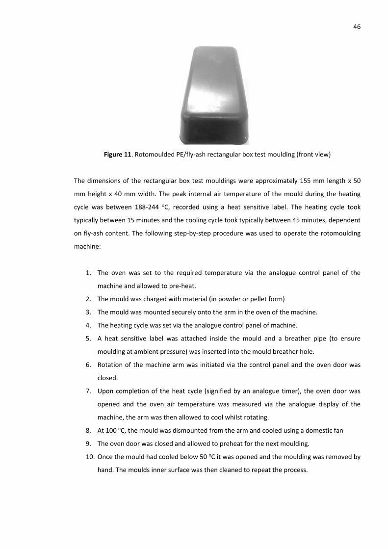
46

Figure 11. Rotomoulded PE/fly-ash rectangular box test moulding (front view)

The dimensions of the rectangular box test mouldings were approximately 155 mm length x 50

mm height x 40 mm width. The peak internal air temperature of the mould during the heating

cycle was between 188-244 oC, recorded using a heat sensitive label. The heating cycle took

typically between 15 minutes and the cooling cycle took typically between 45 minutes, dependent

on fly-ash content. The following step-by-step procedure was used to operate the rotomoulding

machine:

1. The oven was set to the required temperature via the analogue control panel of the

machine and allowed to pre-heat.

2. The mould was charged with material (in powder or pellet form)

3. The mould was mounted securely onto the arm in the oven of the machine.

4. The heating cycle was set via the analogue control panel of machine.

5. A heat sensitive label was attached inside the mould and a breather pipe (to ensure

moulding at ambient pressure) was inserted into the mould breather hole.

6. Rotation of the machine arm was initiated via the control panel and the oven door was

closed.

7. Upon completion of the heat cycle (signified by an analogue timer), the oven door was

opened and the oven air temperature was measured via the analogue display of the

machine, the arm was then allowed to cool whilst rotating.

8. At 100 oC, the mould was dismounted from the arm and cooled using a domestic fan

9. The oven door was closed and allowed to preheat for the next moulding.

10. Once the mould had cooled below 50 oC it was opened and the moulding was removed by

hand. The moulds inner surface was then cleaned to repeat the process.

47 Shot charges for the rectangular box test mouldings were in pellet form. Shot weights were

calculated based on a 3 mm target wall thickness (to conform to the box’s original dimensions)

using Equation 16.

𝑀𝑠 = 𝑎𝑡𝜌 Equation 16.

Where:

Ms = Shot charge mass (kg)

a = Surface area of part (m2)

t = Intended wall thickness (m)

𝜌 = Density of material (kg m-3)

4.5.5 Commercial-scale rotational moulding of unfilled PE and PE/fly-ash safety steps

Safety steps (Figure 12) were rotomoulded using a 1981 ORME 10-arm 6-plate single shuttle

machine fitted with a K-paq temperature logger for process monitoring. The peak internal air

temperature of the mould during the heating cycle varied between 170-215 oC and took typically

between 15-35 minutes. The cooling cycle took typically between 60-90 minutes. Both heating

and cooling cycle times were dependent upon material type. The following step-by-step

procedure was used to operate the machine:

1. The oven was set to the required temperature via the analogue control panel of the

machine and allowed to pre-heat.

2. The safety step mould and temperature logger were then mounted onto the arm of

the machine in the cooling station.

3. Cooling and heating cycles were then set via the analogue control panel of machine.

4. The safety step mould lid was opened, charged with material (in powder or pellet

form) and clamped to close.

5. A breather pipe (to ensure moulding at ambient pressure) was inserted into the

mould tool breather hole along with the thermocouple for the temperature logger.

6. Rotation of the machine arm was initiated via the control panel of the machine and

the oven door was opened.

7. The rotating arm was moved into the oven via the analogue control panel of the

machine for the heat cycle.

8. Upon completing the heat cycle (signified by a ringing bell), the oven door was

opened and the arm was moved back into the cooling station and allowed to cool

whilst rotating. Ceiling mounted fans above the cooling station were running,

48

however, due to the heat generated by the nearby oven, the cooling station air

temperature was approximately 37 0C.

9. Once cooled, the mould tool was opened and the moulding was gently removed using

a crowbar.

10. The moulds inner surface was wiped with a damp cloth to remove any remaining

particles and charged with material again to repeat the process.

Replicate steps were cut in half (lengthways) 24 hours after production for wall thickness

measurements in the corners and the mid-point of the top and bottom surfaces (Figure 13).

Figure 12. The rotomoulded safety step. The overall dimensions of the safety step were

approximately 485 x 280 x 195 mm.

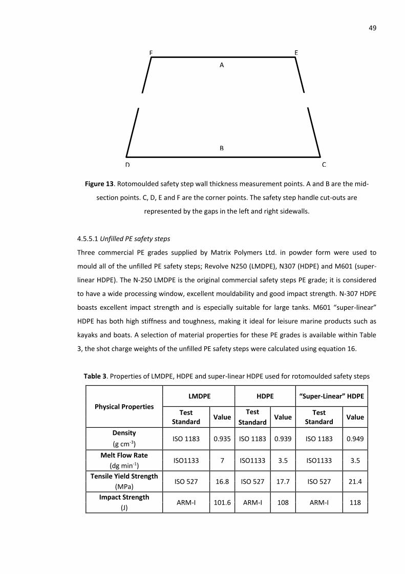
49

Figure 13. Rotomoulded safety step wall thickness measurement points. A and B are the mid-

section points. C, D, E and F are the corner points. The safety step handle cut-outs are

represented by the gaps in the left and right sidewalls.

4.5.5.1 Unfilled PE safety steps

Three commercial PE grades supplied by Matrix Polymers Ltd. in powder form were used to

mould all of the unfilled PE safety steps; Revolve N250 (LMDPE), N307 (HDPE) and M601 (super-

linear HDPE). The N-250 LMDPE is the original commercial safety steps PE grade; it is considered

to have a wide processing window, excellent mouldability and good impact strength. N-307 HDPE

boasts excellent impact strength and is especially suitable for large tanks. M601 “super-linear”

HDPE has both high stiffness and toughness, making it ideal for leisure marine products such as

kayaks and boats. A selection of material properties for these PE grades is available within Table

3, the shot charge weights of the unfilled PE safety steps were calculated using equation 16.

Table 3. Properties of LMDPE, HDPE and super-linear HDPE used for rotomoulded safety steps

Physical Properties

LMDPE HDPE “Super-Linear” HDPE

Test Standard

Value Test

Value Test

Standard Value

Standard

Density ISO 1183 0.935 ISO 1183 0.939 ISO 1183 0.949

(g cm-3)

Melt Flow Rate ISO1133 7 ISO1133 3.5 ISO1133 3.5

(dg min-1)

Tensile Yield Strength ISO 527 16.8 ISO 527 17.7 ISO 527 21.4

(MPa)

Impact Strength ARM-I 101.6 ARM-I 108 ARM-I 118

(J)

A

C D

B

E F

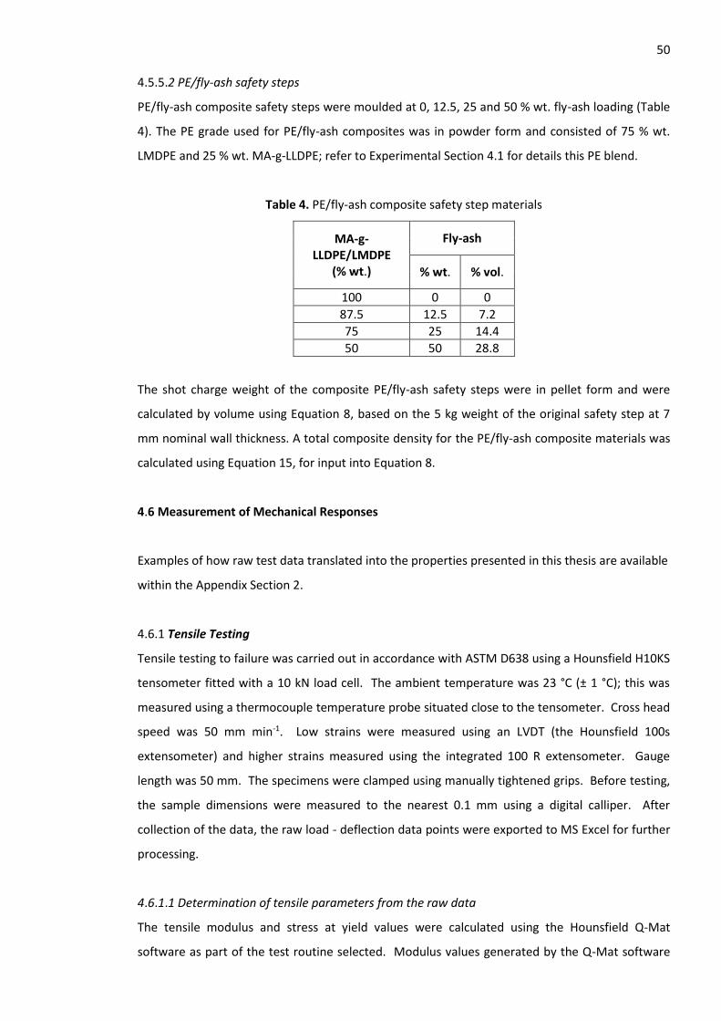
50 4.5.5.2 PE/fly-ash safety steps

PE/fly-ash composite safety steps were moulded at 0, 12.5, 25 and 50 % wt. fly-ash loading (Table

4). The PE grade used for PE/fly-ash composites was in powder form and consisted of 75 % wt.

LMDPE and 25 % wt. MA-g-LLDPE; refer to Experimental Section 4.1 for details this PE blend.

Table 4. PE/fly-ash composite safety step materials

MA-g-LLDPE/LMDPE

(% wt.)

Fly-ash

% wt. % vol.

100 0 0

87.5 12.5 7.2

75 25 14.4

50 50 28.8

The shot charge weight of the composite PE/fly-ash safety steps were in pellet form and were

calculated by volume using Equation 8, based on the 5 kg weight of the original safety step at 7

mm nominal wall thickness. A total composite density for the PE/fly-ash composite materials was

calculated using Equation 15, for input into Equation 8.

4.6 Measurement of Mechanical Responses

Examples of how raw test data translated into the properties presented in this thesis are available

within the Appendix Section 2.

4.6.1 Tensile Testing

Tensile testing to failure was carried out in accordance with ASTM D638 using a Hounsfield H10KS

tensometer fitted with a 10 kN load cell. The ambient temperature was 23 °C (± 1 °C); this was

measured using a thermocouple temperature probe situated close to the tensometer. Cross head

speed was 50 mm min-1. Low strains were measured using an LVDT (the Hounsfield 100s

extensometer) and higher strains measured using the integrated 100 R extensometer. Gauge

length was 50 mm. The specimens were clamped using manually tightened grips. Before testing,

the sample dimensions were measured to the nearest 0.1 mm using a digital calliper. After

collection of the data, the raw load - deflection data points were exported to MS Excel for further

processing.

4.6.1.1 Determination of tensile parameters from the raw data

The tensile modulus and stress at yield values were calculated using the Hounsfield Q-Mat

software as part of the test routine selected. Modulus values generated by the Q-Mat software

51 were checked via linear regression of the raw data and values were found to be similar to those

generated by the software. 8 replicate tensile samples of each material were measured; a

maximum of three outlier results were removed for each parameter to give the five closest

values. Averages and standard deviations were calculated using the five closest values obtained

for each material. It is appreciated that, in a selection of graphs from the results and discussion

section of this report the standard deviation error bars are small relative to the size of the data

point marker, giving the impression that they are absent. However, standard deviation was

calculated throughout this study. Therefore, this data is tabulated within the Appendix Section 3

for selected plots; the relevant table number is provided in the Results and Discussion Sections.

4.6.2 Flexural testing

Flexural testing (in three point bend mode according to ATSM D790) was carried out to 10 mm

deflection using a Hounsfield H10KS tensometer fitted with a 1 kN load cell. The ambient

temperature was 23 °C (± 1 °C); this was measured using a thermocouple temperature probe

situated close to the tensometer. The span between the sample supports was 64 mm, crosshead

speed was 5 mm min-1 and a 0.05 N preload was applied before collecting data. Force and

crosshead displacement were recorded up to failure and the crosshead auto-returned to the start

position.

4.6.2.1 Determination of flexural parameters from the raw data

The raw load deflection data from the three point bend tests was first converted in to stress (in

outer fibre) versus strain (in outer fibre) data using equations 17 and 18 respectively. Calculations

were performed using MS Excel. The parameters determined from flexural stress-strain data were

the secant modulus at 1 % strain (Esf(1%)), the flexural modulus (Ef) and the flexural stress at 10 mm

deflection, yield or break (Eσ).

𝜎𝑓 = 3𝑃𝐿

2𝑏𝑑2 Equation 17.

Where:

σf = Stress in outer fibre at mid-span

P = Load at a given point on the load deflection curve

d = Depth of tested beam

b = Width of tested beam

L = Support span

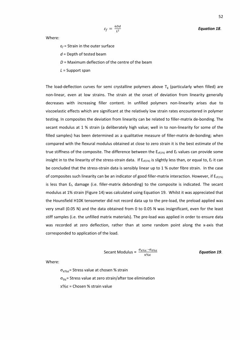
52

휀𝑓 = 6𝐷𝑑

𝐿2 Equation 18.

Where:

εf = Strain in the outer surface

d = Depth of tested beam

D = Maximum deflection of the centre of the beam

L = Support span

The load-deflection curves for semi crystalline polymers above Tg (particularly when filled) are

non-linear, even at low strains. The strain at the onset of deviation from linearity generally

decreases with increasing filler content. In unfilled polymers non-linearity arises due to

viscoelastic effects which are significant at the relatively low strain rates encountered in polymer

testing. In composites the deviation from linearity can be related to filler-matrix de-bonding. The

secant modulus at 1 % strain (a deliberately high value; well in to non-linearity for some of the

filled samples) has been determined as a qualitative measure of filler-matrix de-bonding; when

compared with the flexural modulus obtained at close to zero strain it is the best estimate of the

true stiffness of the composite. The difference between the Esf(1%) and Ef values can provide some

insight in to the linearity of the stress-strain data. If Esf(1%) is slightly less than, or equal to, Ef it can

be concluded that the stress-strain data is sensibly linear up to 1 % outer fibre strain. In the case

of composites such linearity can be an indicator of good filler-matrix interaction. However, if Esf(1%)

is less than Ef, damage (i.e. filler-matrix debonding) to the composite is indicated. The secant

modulus at 1% strain (Figure 14) was calculated using Equation 19. Whilst it was appreciated that

the Hounsfield H10K tensometer did not record data up to the pre-load, the preload applied was

very small (0.05 N) and the data obtained from 0 to 0.05 N was insignificant, even for the least

stiff samples (i.e. the unfilled matrix materials). The pre-load was applied in order to ensure data

was recorded at zero deflection, rather than at some random point along the x-axis that

corresponded to application of the load.

Secant Modulus = σx%ε –σ0%ε

x%ε Equation 19.

Where:

σx%ε= Stress value at chosen % strain

σ0ε= Stress value at zero strain/after toe elimination

x%ε = Chosen % strain value

53

Figure 14. The difference between flexural modulus and secant modulus at chosen strain.

The flexural modulus was calculated from linear regression of the first 10 stress versus strain data

points which showed the highest rate of change. The latter was checked by plotting the first 200

data points and checking the region of maximum slope; this usually occurred from the first

recorded data point thanks to inclusion of a pre-load in the method. However, there were cases

where the sample was very slightly twisted and small amount of force was required to flatten the

sample on its supports. In such cases, the maximum rate of increase in stress was some distance

from the first recorded data point and an appropriate compensation was made. The flexural

stress at 10 mm deflection was calculated by Hounsfield’s QMAT tensometer software. 8 replicate

flexural samples of each material were measured; a maximum of three outlier results were

removed for the secant modulus at 1 % strain , flexural modulus and flexural stress at 10mm

deflection to give the five closest values of each parameter. Averages and standard deviations

were calculated using the five closest values obtained for each material.

4.6.3 High temperature flexural testing of PE/fly-ash composites

Flexural testing to 10 mm deflection (in three point bend mode) at 85, 100, and 115 oC was

carried out in accordance with ATSM D790 using a Hounsfield HTE50 tensometer fitted with a 50

kN load cell and a heat chamber containing a 3 point bend test rig. The heat chamber

temperature was controlled via the tensometers computer. The span between the sample

supports was 64 mm, crosshead speed was 5 mm min-1 and a 0.05 N preload was applied before

54 collecting data. Force and crosshead displacement were recorded up to failure and the crosshead

auto-returned to the start position.

4.6.3.1 Determination of flexural parameters from the raw data

The flexural modulus was calculated by Hounsfield’s QMAT tensometer software. Section 4.6.2.1

describes the procedure to determine the flexural stress at 10 mm deflection for the PE/fly-ash

composite materials.

4.6.4. Poisson’s ratio testing of PE/fly-ash composites

Poisson’s ratio determination of the PE/fly-ash composite safety step materials was carried out

using the advanced video extensometer at the National Composites Certification and Evaluation

Facility (NCCEF) within the University of Manchester. 5 tensile test pieces were cut from PE/fly-

ash composite plaques via an OMAX water jet cutter, using the built in CAD package within the

control system of the machine (Section 4.5.1). Sample dimensions were programmed to be 195 x

35 x 3.5 mm with a gauge section of 80 x 25 mm. The thickness varied between 3-4 mm

(depending upon filler content). Specimens were dried in a Carbolite electric oven at 50 oC for 3

hours to evaporate any water potentially absorbed by the composite during the water jet cutting

process. Individual specimens were measured to the nearest 0.001 mm before testing. Tensile

testing to failure was carried out in accordance with ASTM D638-10 using an Instron 5982

tensometer fitted with a 100 kN load cell. The specimens were held using hydraulic grips. Cross

head speed was 5 mm min-1. Axial and transverse strains were measured using an Instron AVE

2663-821 video extensometer at 10 samples per second. The system was controlled using

Instron’s Bluehill software. Test pieces were marked on the centre of their gauge lengths with a

permanent pen using both vertical and horizontal dots in the four principal directions. The

markings provided a reference grid for the video extensometer to measure strain in the axial and

transverse directions during the test. The ambient temperature was 23 °C (± 1 °C); this was

measured using a thermocouple temperature probe situated close to the tensometer. After

collection of the data, the numerical axial and transverse strain data points were exported to MS

Excel for further processing.

4.6.4.1 Determination of Poisson’s ratio from the raw data

The transverse and axial strain of the test specimens (to failure) was provided by the tensometers

integrated computer in % format. Equation 20 was then used to calculate a value of Poisson’s

ratio at every point of strain (up to the yield point) using MS Excel.

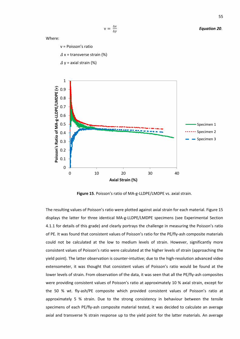
55

ν = ∆𝑥

∆𝑦 Equation 20.

Where:

ν = Poisson’s ratio

𝛥 x = transverse strain (%)

𝛥 y = axial strain (%)

Figure 15. Poisson’s ratio of MA-g-LLDPE/LMDPE vs. axial strain.

The resulting values of Poisson’s ratio were plotted against axial strain for each material. Figure 15

displays the latter for three identical MA-g-LLDPE/LMDPE specimens (see Experimental Section

4.1.1 for details of this grade) and clearly portrays the challenge in measuring the Poisson’s ratio

of PE. It was found that consistent values of Poisson’s ratio for the PE/fly-ash composite materials

could not be calculated at the low to medium levels of strain. However, significantly more

consistent values of Poisson’s ratio were calculated at the higher levels of strain (approaching the

yield point). The latter observation is counter-intuitive; due to the high-resolution advanced video

extensometer, it was thought that consistent values of Poisson’s ratio would be found at the

lower levels of strain. From observation of the data, it was seen that all the PE/fly-ash composites

were providing consistent values of Poisson’s ratio at approximately 10 % axial strain, except for

the 50 % wt. fly-ash/PE composite which provided consistent values of Poisson’s ratio at

approximately 5 % strain. Due to the strong consistency in behaviour between the tensile

specimens of each PE/fly-ash composite material tested, it was decided to calculate an average

axial and transverse % strain response up to the yield point for the latter materials. An average

0

0.1

0.2

0.3

0.4

0.5

0.6

0.7

0.8

0.9

1

0 10 20 30 40

Po

isso

n's

Rat

io o

f M

A-g

-LLD

PE/

LMD

PE

(ν)

Axial Strain (%)

Specimen 1

Specimen 2

Specimen 3

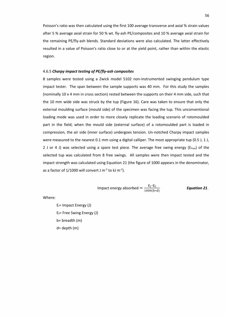
56 Poisson’s ratio was then calculated using the first 100 average transverse and axial % strain values

after 5 % average axial strain for 50 % wt. fly-ash PE/composites and 10 % average axial strain for

the remaining PE/fly-ash blends. Standard deviations were also calculated. The latter effectively

resulted in a value of Poisson’s ratio close to or at the yield point, rather than within the elastic

region.

4.6.5 Charpy impact testing of PE/fly-ash composites

8 samples were tested using a Zwick model 5102 non-instrumented swinging pendulum type

impact tester. The span between the sample supports was 40 mm. For this study the samples

(nominally 10 x 4 mm in cross section) rested between the supports on their 4 mm side, such that

the 10 mm wide side was struck by the tup (Figure 16). Care was taken to ensure that only the

external moulding surface (mould side) of the specimen was facing the tup. This unconventional

loading mode was used in order to more closely replicate the loading scenario of rotomoulded

part in the field; when the mould side (external surface) of a rotomoulded part is loaded in

compression, the air side (inner surface) undergoes tension. Un-notched Charpy impact samples

were measured to the nearest 0.1 mm using a digital calliper. The most appropriate tup (0.5 J, 1 J,

2 J or 4 J) was selected using a spare test piece. The average free swing energy (Efree) of the

selected tup was calculated from 8 free swings. All samples were then impact tested and the

impact strength was calculated using Equation 21 (the figure of 1000 appears in the denominator,

as a factor of 1/1000 will convert J m-2 to kJ m-2).

Impact energy absorbed =Ei–Ef

1000(b∗d) Equation 21.

Where:

Ei= Impact Energy (J)

Ef= Free Swing Energy (J)

b= breadth (m)

d= depth (m)

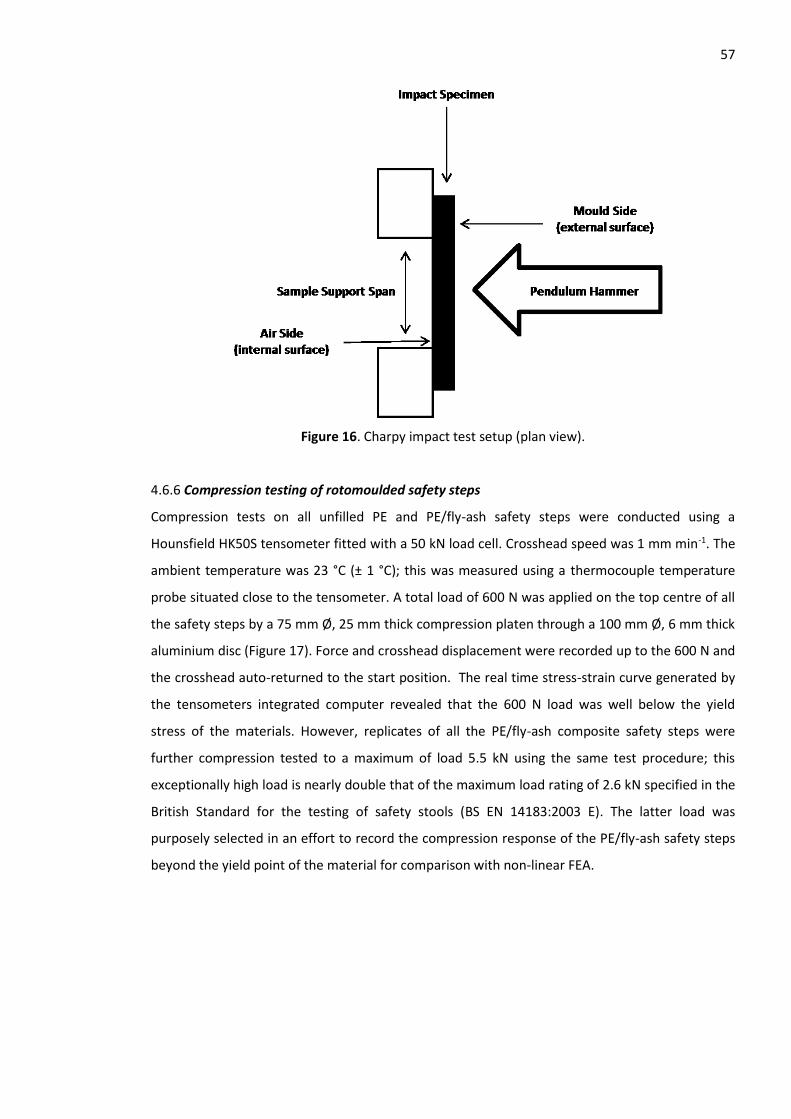
57

Figure 16. Charpy impact test setup (plan view).

4.6.6 Compression testing of rotomoulded safety steps

Compression tests on all unfilled PE and PE/fly-ash safety steps were conducted using a

Hounsfield HK50S tensometer fitted with a 50 kN load cell. Crosshead speed was 1 mm min-1. The

ambient temperature was 23 °C (± 1 °C); this was measured using a thermocouple temperature

probe situated close to the tensometer. A total load of 600 N was applied on the top centre of all

the safety steps by a 75 mm Ø, 25 mm thick compression platen through a 100 mm Ø, 6 mm thick

aluminium disc (Figure 17). Force and crosshead displacement were recorded up to the 600 N and

the crosshead auto-returned to the start position. The real time stress-strain curve generated by

the tensometers integrated computer revealed that the 600 N load was well below the yield

stress of the materials. However, replicates of all the PE/fly-ash composite safety steps were

further compression tested to a maximum of load 5.5 kN using the same test procedure; this

exceptionally high load is nearly double that of the maximum load rating of 2.6 kN specified in the

British Standard for the testing of safety stools (BS EN 14183:2003 E). The latter load was

purposely selected in an effort to record the compression response of the PE/fly-ash safety steps

beyond the yield point of the material for comparison with non-linear FEA.

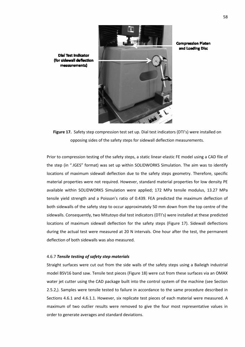
58

Figure 17. Safety step compression test set up. Dial test indicators (DTI’s) were installed on

opposing sides of the safety steps for sidewall deflection measurements.

Prior to compression testing of the safety steps, a static linear-elastic FE model using a CAD file of

the step (in “.IGES” format) was set up within SOLIDWORKS Simulation. The aim was to identify

locations of maximum sidewall deflection due to the safety steps geometry. Therefore, specific

material properties were not required. However, standard material properties for low density PE

available within SOLIDWORKS Simulation were applied; 172 MPa tensile modulus, 13.27 MPa

tensile yield strength and a Poisson’s ratio of 0.439. FEA predicted the maximum deflection of

both sidewalls of the safety step to occur approximately 50 mm down from the top centre of the

sidewalls. Consequently, two Mitutoyo dial test indicators (DTI’s) were installed at these predicted

locations of maximum sidewall deflection for the safety steps (Figure 17). Sidewall deflections

during the actual test were measured at 20 N intervals. One hour after the test, the permanent

deflection of both sidewalls was also measured.

4.6.7 Tensile testing of safety step materials

Straight surfaces were cut out from the side walls of the safety steps using a Baileigh industrial

model BSV16 band saw. Tensile test pieces (Figure 18) were cut from these surfaces via an OMAX

water jet cutter using the CAD package built into the control system of the machine (see Section

2.5.2,). Samples were tensile tested to failure in accordance to the same procedure described in

Sections 4.6.1 and 4.6.1.1. However, six replicate test pieces of each material were measured. A

maximum of two outlier results were removed to give the four most representative values in

order to generate averages and standard deviations.

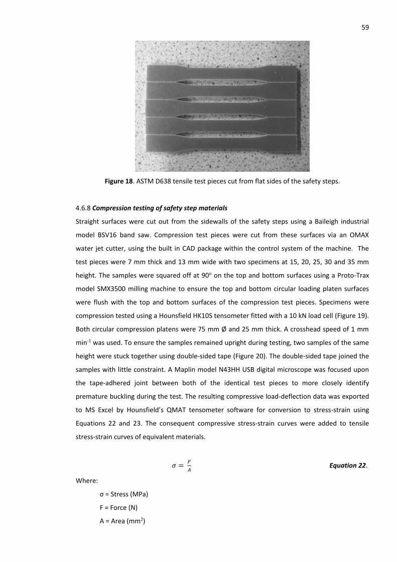
59

Figure 18. ASTM D638 tensile test pieces cut from flat sides of the safety steps.

4.6.8 Compression testing of safety step materials

Straight surfaces were cut out from the sidewalls of the safety steps using a Baileigh industrial

model BSV16 band saw. Compression test pieces were cut from these surfaces via an OMAX

water jet cutter, using the built in CAD package within the control system of the machine. The

test pieces were 7 mm thick and 13 mm wide with two specimens at 15, 20, 25, 30 and 35 mm

height. The samples were squared off at 90o on the top and bottom surfaces using a Proto-Trax

model SMX3500 milling machine to ensure the top and bottom circular loading platen surfaces

were flush with the top and bottom surfaces of the compression test pieces. Specimens were

compression tested using a Hounsfield HK10S tensometer fitted with a 10 kN load cell (Figure 19).

Both circular compression platens were 75 mm Ø and 25 mm thick. A crosshead speed of 1 mm

min-1 was used. To ensure the samples remained upright during testing, two samples of the same

height were stuck together using double-sided tape (Figure 20). The double-sided tape joined the

samples with little constraint. A Maplin model N43HH USB digital microscope was focused upon

the tape-adhered joint between both of the identical test pieces to more closely identify

premature buckling during the test. The resulting compressive load-deflection data was exported

to MS Excel by Hounsfield’s QMAT tensometer software for conversion to stress-strain using

Equations 22 and 23. The consequent compressive stress-strain curves were added to tensile

stress-strain curves of equivalent materials.

𝜎 = 𝐹

𝐴 Equation 22.

Where:

σ = Stress (MPa)

F = Force (N)

A = Area (mm2)

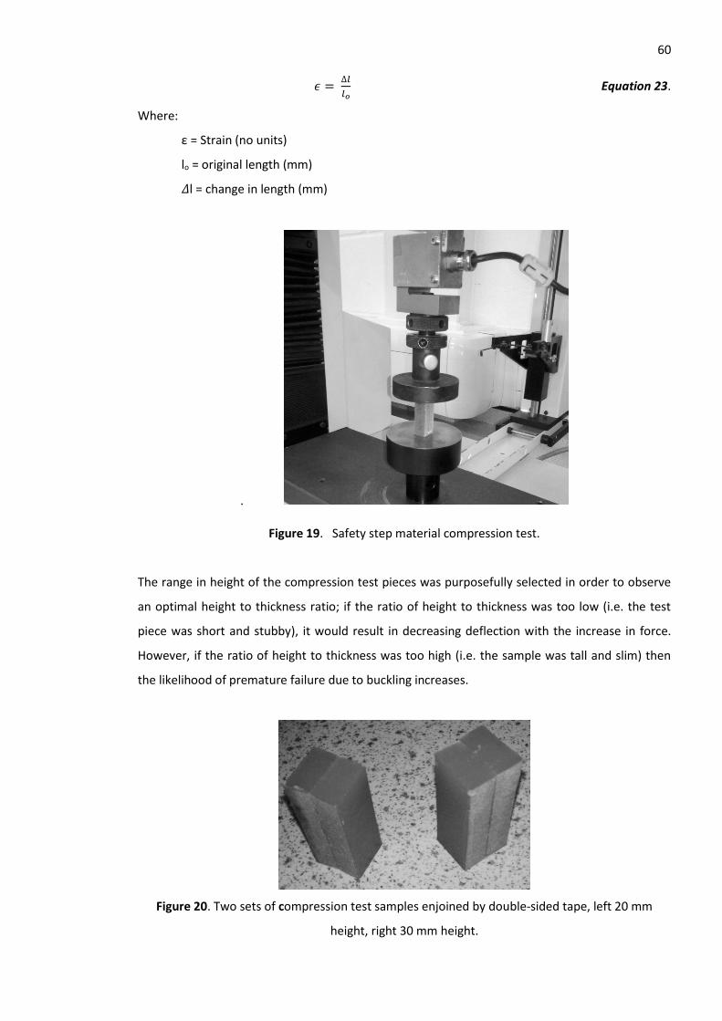
60

𝜖 = ∆𝑙

𝑙𝑜 Equation 23.

Where:

ε = Strain (no units)

lo = original length (mm)

𝛥l = change in length (mm)

.

Figure 19. Safety step material compression test.

The range in height of the compression test pieces was purposefully selected in order to observe

an optimal height to thickness ratio; if the ratio of height to thickness was too low (i.e. the test

piece was short and stubby), it would result in decreasing deflection with the increase in force.

However, if the ratio of height to thickness was too high (i.e. the sample was tall and slim) then

the likelihood of premature failure due to buckling increases.

Figure 20. Two sets of compression test samples enjoined by double-sided tape, left 20 mm

height, right 30 mm height.

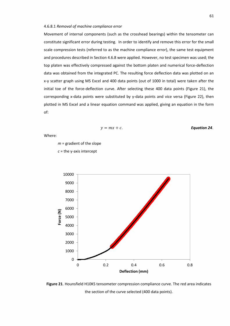
61 4.6.8.1 Removal of machine compliance error

Movement of internal components (such as the crosshead bearings) within the tensometer can

constitute significant error during testing. In order to identify and remove this error for the small

scale compression tests (referred to as the machine compliance error), the same test equipment

and procedures described in Section 4.6.8 were applied. However, no test specimen was used; the

top platen was effectively compressed against the bottom platen and numerical force-deflection

data was obtained from the integrated PC. The resulting force deflection data was plotted on an

x-y scatter graph using MS Excel and 400 data points (out of 1000 in total) were taken after the

initial toe of the force-deflection curve. After selecting these 400 data points (Figure 21), the

corresponding x-data points were substituted by y-data points and vice versa (Figure 22), then

plotted in MS Excel and a linear equation command was applied, giving an equation in the form

of:

𝑦 = 𝑚𝑥 + 𝑐. Equation 24.

Where:

m = gradient of the slope

c = the y-axis intercept

Figure 21. Hounsfield H10KS tensometer compression compliance curve. The red area indicates

the section of the curve selected (400 data points).

0

1000

2000

3000

4000

5000

6000

7000

8000

9000

10000

0 0.2 0.4 0.6 0.8

Forc

e (N

)

Deflection (mm)

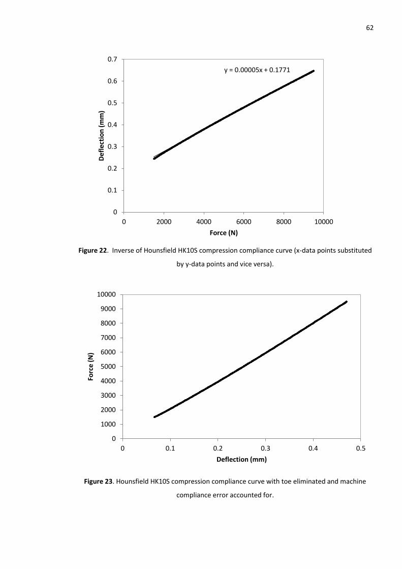
62

Figure 22. Inverse of Hounsfield HK10S compression compliance curve (x-data points substituted

by y-data points and vice versa).

Figure 23. Hounsfield HK10S compression compliance curve with toe eliminated and machine

compliance error accounted for.

y = 0.00005x + 0.1771

0

0.1

0.2

0.3

0.4

0.5

0.6

0.7

0 2000 4000 6000 8000 10000

De

flec

tio

n (

mm

)

Force (N)

0

1000

2000

3000

4000

5000

6000

7000

8000

9000

10000

0 0.1 0.2 0.3 0.4 0.5

Forc

e (N

)

Deflection (mm)

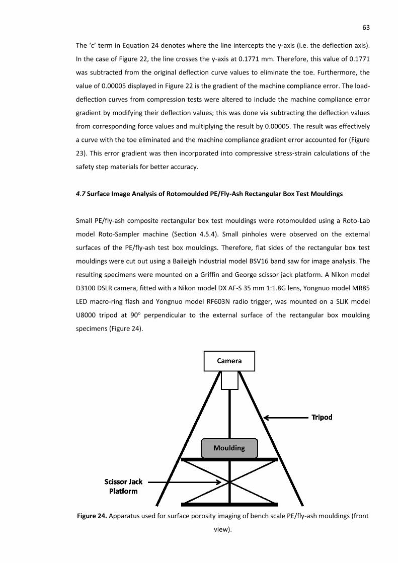
63 The ‘c’ term in Equation 24 denotes where the line intercepts the y-axis (i.e. the deflection axis).

In the case of Figure 22, the line crosses the y-axis at 0.1771 mm. Therefore, this value of 0.1771

was subtracted from the original deflection curve values to eliminate the toe. Furthermore, the

value of 0.00005 displayed in Figure 22 is the gradient of the machine compliance error. The load-

deflection curves from compression tests were altered to include the machine compliance error

gradient by modifying their deflection values; this was done via subtracting the deflection values

from corresponding force values and multiplying the result by 0.00005. The result was effectively

a curve with the toe eliminated and the machine compliance gradient error accounted for (Figure

23). This error gradient was then incorporated into compressive stress-strain calculations of the

safety step materials for better accuracy.

4.7 Surface Image Analysis of Rotomoulded PE/Fly-Ash Rectangular Box Test Mouldings

Small PE/fly-ash composite rectangular box test mouldings were rotomoulded using a Roto-Lab

model Roto-Sampler machine (Section 4.5.4). Small pinholes were observed on the external

surfaces of the PE/fly-ash test box mouldings. Therefore, flat sides of the rectangular box test

mouldings were cut out using a Baileigh Industrial model BSV16 band saw for image analysis. The

resulting specimens were mounted on a Griffin and George scissor jack platform. A Nikon model

D3100 DSLR camera, fitted with a Nikon model DX AF-S 35 mm 1:1.8G lens, Yongnuo model MR85

LED macro-ring flash and Yongnuo model RF603N radio trigger, was mounted on a SLIK model

U8000 tripod at 90o perpendicular to the external surface of the rectangular box moulding

specimens (Figure 24).

Figure 24. Apparatus used for surface porosity imaging of bench scale PE/fly-ash mouldings (front

view).

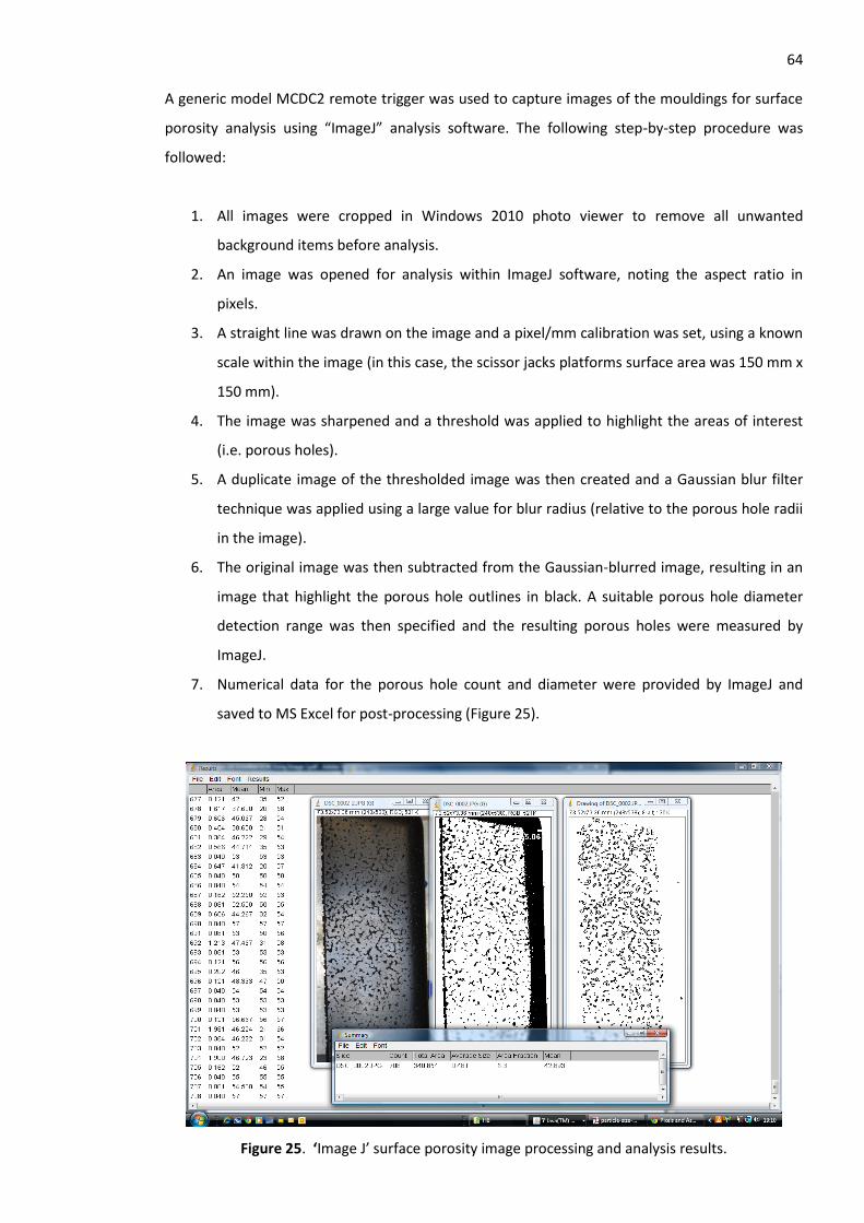
64 A generic model MCDC2 remote trigger was used to capture images of the mouldings for surface

porosity analysis using “ImageJ” analysis software. The following step-by-step procedure was

followed:

1. All images were cropped in Windows 2010 photo viewer to remove all unwanted

background items before analysis.

2. An image was opened for analysis within ImageJ software, noting the aspect ratio in

pixels.

3. A straight line was drawn on the image and a pixel/mm calibration was set, using a known

scale within the image (in this case, the scissor jacks platforms surface area was 150 mm x

150 mm).

4. The image was sharpened and a threshold was applied to highlight the areas of interest

(i.e. porous holes).

5. A duplicate image of the thresholded image was then created and a Gaussian blur filter

technique was applied using a large value for blur radius (relative to the porous hole radii

in the image).

6. The original image was then subtracted from the Gaussian-blurred image, resulting in an

image that highlight the porous hole outlines in black. A suitable porous hole diameter

detection range was then specified and the resulting porous holes were measured by

ImageJ.

7. Numerical data for the porous hole count and diameter were provided by ImageJ and

saved to MS Excel for post-processing (Figure 25).

Figure 25. ‘Image J’ surface porosity image processing and analysis results.

65 4.8 Scanning Electron Microscopy and Energy Dispersive X-ray Analysis

Scanning electron microscopy (SEM) permits the observation and characterisation of various

heterogeneous organic and inorganic materials on a micrometer (μm) to nanometer (ηm) scale

[213], typically producing images at magnifications of up to 106x [214]. During SEM, an area or

volume of a sample is irradiated with a precisely focused electron beam that can be swept in a

raster fashion to image an entire sample or statically focused to image a specific point on a

sample. Various signals such as secondary electrons, backscattered electrons and x-rays are

emitted from atoms in the sample upon interaction with the electron beam [215]. These signals are

used to analyse various characteristics of the sample such as surface topography and elemental

composition. With regards to surface imaging, the signals of most interest are the secondary and

backscattered electrons as they are emitted due to differences in the surface topography of the

sample [216].

With regards to elemental composition, the signals of most interest are x-ray emissions; the

atoms in a sample have a unique a set of peaks on the x-ray emission spectrum [217]. Upon

excitation of an atom by an external source of charged particles (i.e. an electron or proton beam)

an electron from a low-energy inner shell is ejected, prompting an electron replacement from a

high-energy outer shell. The difference in energy between the inner and outer shells of the atom

is released in the form of x-rays [218]. The number and energy of x-rays are detected by an energy

dispersive spectrometer integrated with the SEM. X-ray emissions are a product of the difference

in energy between the two shells and the atomic structure of the elements in the sample [219].

Therefore, the elemental composition of a sample can be identified from x-ray emissions. The

latter process is called energy dispersive x-ray (EDX) analysis.

SEM was used to image the filler particles and fracture surfaces of tensile test specimens. EDX

analysis was used to determine the elemental composition of the fillers. The latter was achieved

by a Jeol model JSM 5600 SEM fitted with an Oxford instruments 7800 series EDX detector.

4.8.1 Sample preparation

1. A double sided self-adhesive carbon pad was stuck on to the specimen face of a fresh stub

and the protective film removed, exposing the adhesive surface attached to the stub.

2. A small amount of the filler sample was sprinkled on to the pad and the excess removed

with a jet of compressed air.

3. The sample was then sputter coated with gold to render its surfaces electrically

conductive and reduce the tendency to charge.

66 4.8.2 Scanning electron microscope and energy dispersive x-ray operating conditions

For the filler particle surface imaging, the SEM was run at an accelerating voltage of 15 kV, using

the secondary electron detector. Digital images of each specimen were acquired at a range of

magnifications. Care was taken to ensure that the image was representative of the sample. EDX

was carried out using spot analysis with an accelerating voltage of 15 kV, the spot size was

adjusted to provide an acceptable detector dead time in the region of approximately 30 %. The

levels of all the elements detected were recorded. To ensure that the data was representative,

three replicate areas were examined and the data averaged.

4.9 Differential Scanning Calorimetry

Differential scanning calorimetry (DSC) was conducted to investigate the effect of blending

method and filler addition on the melting, crystallisation and re-melting of the PE based matrix

materials developed for this PhD study. DSC is defined by Höhne et al. as a method of measuring

the change of the difference in heat flow rate to a sample and a reference sample during a

controlled temperature program [220]. It is a method of measuring the thermal transitions of a

material. In principle, DSC converts a temperature difference to an energy per unit mass value

associated with a phase transition of a material (e.g. the energy per unit mass required to melt a

solid material to a liquid) [221]. DSC is widely applied to polymeric materials to analyse their

microstructural properties. The melting temperature (Tm) of polymers is dependent upon their

molecular composition, molecular structure and thermal history. Consequently, the percentage

crystallinity of a polymer can be estimated using the melting and crystallisation energy-

temperature peaks from a DSC thermogramme alongside reference heats of fusion found in

literature [222] (refer to Appendix Section 4 for typical DSC thermogramme traces). The melting

point (Tm) of a polymer is defined by the peak of its energy-temperature curve. The heat of fusion

of a polymer is the area under the energy-temperature peak from the beginning to the end of the

baseline. The crystallinity of the polymer can then be calculated by dividing the measured heat of

fusion by the heat of fusion for an equivalent 100 % crystalline polymer [223] (see Equation 25).

The DSC instrument used for this study was a Perkin-Elmer DSC-7, a power compensation type

instrument. The following heat – hold – cool – heat cycle was used:

Heat from 20 °C to 240 °C at 20 °C min-1

Hold at 240 °C for 5 minutes

Cool from 240 °C to 20 oC at 20 °C min-1

Hold at 20 °C for 2 minutes

67

Heat from 20 °C to 240 °C at 20 °C min-1

Samples were heated in a nitrogen atmosphere (flow rate 30 cm3 min-1). The following

parameters were recorded during DSC:

1st Heat (for determination of the specimens melting characteristics in its as-moulded component)

Onset of melting temperature

Peak melting temperature

Melting temperature range

Heat of fusion (for calculation of crystalline content. The samples were held at 240 oC for

five minutes to ensure complete melting and total eradication of previous thermal

history)

Cool from melt (to provide controlled crystallisation)

Onset of crystallisation temperature

Crystallisation exotherm peak temperature

Crystallisation temperature range

Heat of crystallisation (for calculation of crystalline content obtained during controlled

crystallisation)

2nd Heat (to examine the melting of crystal structures formed as a result of controlled

crystallisation)

The same parameters as recorded during the 1st heat were recorded

Sample mass was typically between 4 and 10 mg. Samples were crimped in to aluminium pans

and the DSC head was purged with nitrogen (flow rate 50 cm3 min-1). The crystalline content of

unfilled PE materials was determined using Equation 25. For PE/filler composites, crystallinity

content was also calculated using Equation 25. However, Equation 26 was used to calculate 𝛥Hf

for input into Equation 25.

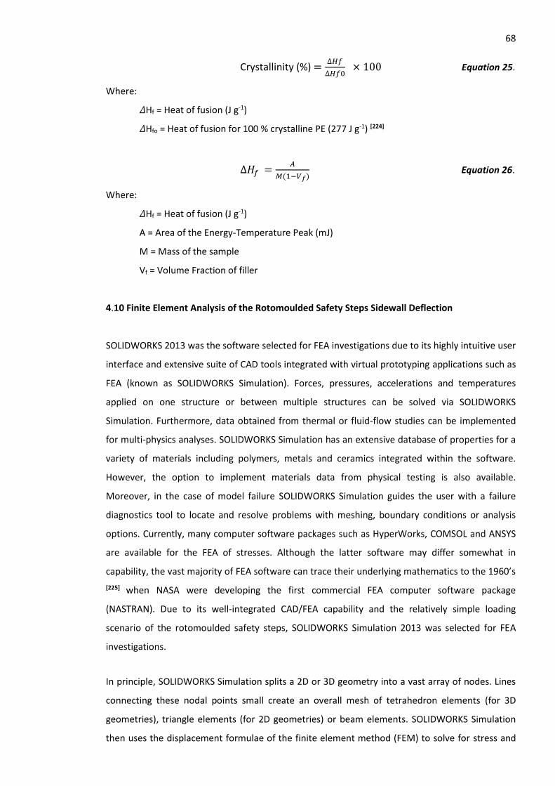
68

Crystallinity (%) =∆𝐻𝑓

∆𝐻𝑓0 × 100 Equation 25.

Where:

𝛥Hf = Heat of fusion (J g-1)

𝛥Hfo = Heat of fusion for 100 % crystalline PE (277 J g-1) [224]

∆𝐻𝑓 =𝐴

𝑀(1−𝑉𝑓) Equation 26.

Where:

𝛥Hf = Heat of fusion (J g-1)

A = Area of the Energy-Temperature Peak (mJ)

M = Mass of the sample

Vf = Volume Fraction of filler

4.10 Finite Element Analysis of the Rotomoulded Safety Steps Sidewall Deflection

SOLIDWORKS 2013 was the software selected for FEA investigations due to its highly intuitive user

interface and extensive suite of CAD tools integrated with virtual prototyping applications such as

FEA (known as SOLIDWORKS Simulation). Forces, pressures, accelerations and temperatures

applied on one structure or between multiple structures can be solved via SOLIDWORKS

Simulation. Furthermore, data obtained from thermal or fluid-flow studies can be implemented

for multi-physics analyses. SOLIDWORKS Simulation has an extensive database of properties for a

variety of materials including polymers, metals and ceramics integrated within the software.

However, the option to implement materials data from physical testing is also available.

Moreover, in the case of model failure SOLIDWORKS Simulation guides the user with a failure

diagnostics tool to locate and resolve problems with meshing, boundary conditions or analysis

options. Currently, many computer software packages such as HyperWorks, COMSOL and ANSYS

are available for the FEA of stresses. Although the latter software may differ somewhat in

capability, the vast majority of FEA software can trace their underlying mathematics to the 1960’s

[225] when NASA were developing the first commercial FEA computer software package

(NASTRAN). Due to its well-integrated CAD/FEA capability and the relatively simple loading

scenario of the rotomoulded safety steps, SOLIDWORKS Simulation 2013 was selected for FEA

investigations.

In principle, SOLIDWORKS Simulation splits a 2D or 3D geometry into a vast array of nodes. Lines

connecting these nodal points small create an overall mesh of tetrahedron elements (for 3D

geometries), triangle elements (for 2D geometries) or beam elements. SOLIDWORKS Simulation

then uses the displacement formulae of the finite element method (FEM) to solve for stress and

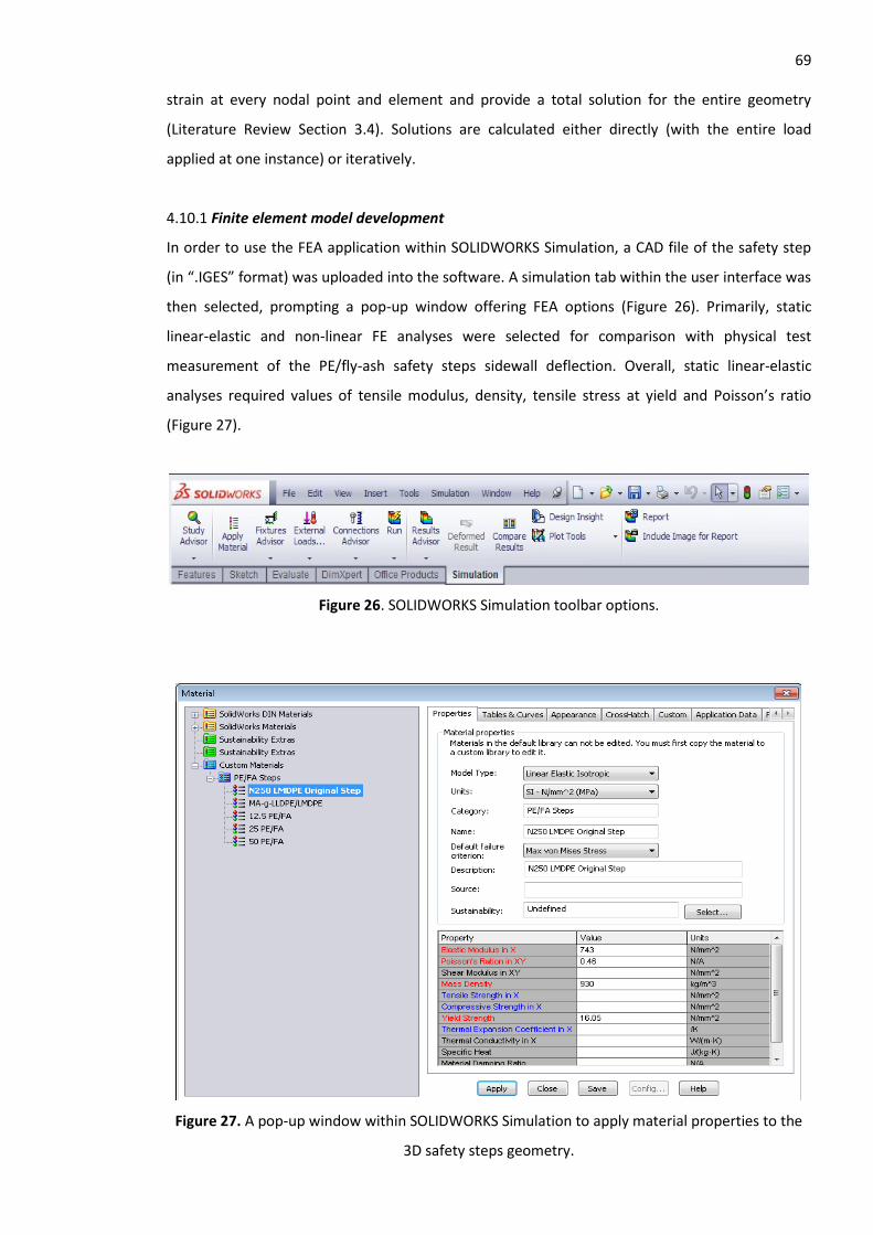
69 strain at every nodal point and element and provide a total solution for the entire geometry

(Literature Review Section 3.4). Solutions are calculated either directly (with the entire load

applied at one instance) or iteratively.

4.10.1 Finite element model development

In order to use the FEA application within SOLIDWORKS Simulation, a CAD file of the safety step

(in “.IGES” format) was uploaded into the software. A simulation tab within the user interface was

then selected, prompting a pop-up window offering FEA options (Figure 26). Primarily, static

linear-elastic and non-linear FE analyses were selected for comparison with physical test

measurement of the PE/fly-ash safety steps sidewall deflection. Overall, static linear-elastic

analyses required values of tensile modulus, density, tensile stress at yield and Poisson’s ratio

(Figure 27).

Figure 26. SOLIDWORKS Simulation toolbar options.

Figure 27. A pop-up window within SOLIDWORKS Simulation to apply material properties to the

3D safety steps geometry.

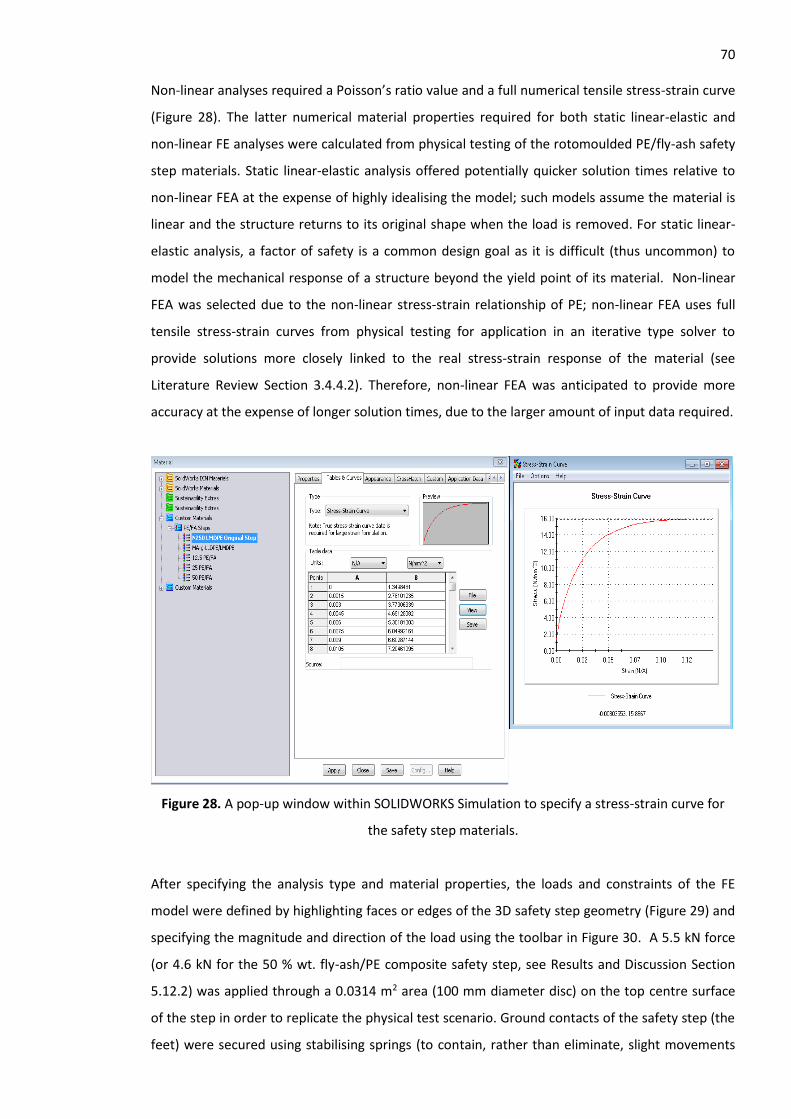
70 Non-linear analyses required a Poisson’s ratio value and a full numerical tensile stress-strain curve

(Figure 28). The latter numerical material properties required for both static linear-elastic and

non-linear FE analyses were calculated from physical testing of the rotomoulded PE/fly-ash safety

step materials. Static linear-elastic analysis offered potentially quicker solution times relative to

non-linear FEA at the expense of highly idealising the model; such models assume the material is

linear and the structure returns to its original shape when the load is removed. For static linear-

elastic analysis, a factor of safety is a common design goal as it is difficult (thus uncommon) to

model the mechanical response of a structure beyond the yield point of its material. Non-linear

FEA was selected due to the non-linear stress-strain relationship of PE; non-linear FEA uses full

tensile stress-strain curves from physical testing for application in an iterative type solver to

provide solutions more closely linked to the real stress-strain response of the material (see

Literature Review Section 3.4.4.2). Therefore, non-linear FEA was anticipated to provide more

accuracy at the expense of longer solution times, due to the larger amount of input data required.

Figure 28. A pop-up window within SOLIDWORKS Simulation to specify a stress-strain curve for

the safety step materials.

After specifying the analysis type and material properties, the loads and constraints of the FE

model were defined by highlighting faces or edges of the 3D safety step geometry (Figure 29) and

specifying the magnitude and direction of the load using the toolbar in Figure 30. A 5.5 kN force

(or 4.6 kN for the 50 % wt. fly-ash/PE composite safety step, see Results and Discussion Section

5.12.2) was applied through a 0.0314 m2 area (100 mm diameter disc) on the top centre surface

of the step in order to replicate the physical test scenario. Ground contacts of the safety step (the

feet) were secured using stabilising springs (to contain, rather than eliminate, slight movements

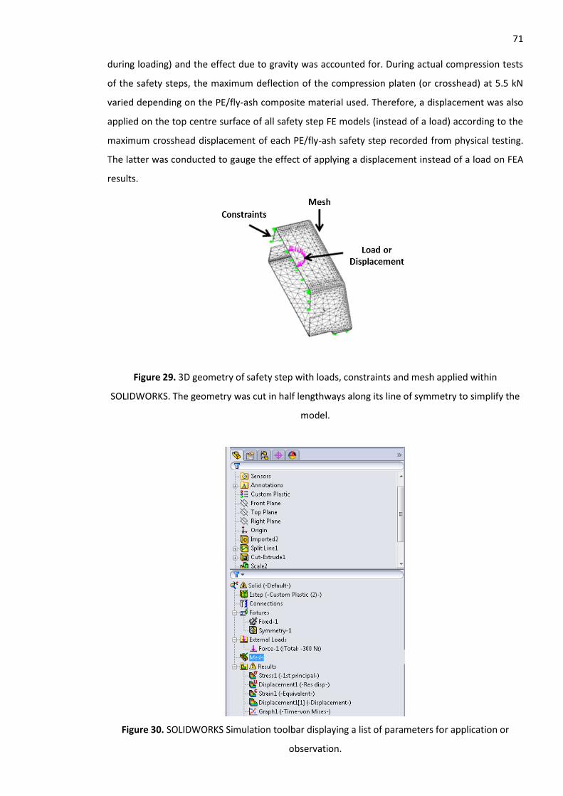
71 during loading) and the effect due to gravity was accounted for. During actual compression tests

of the safety steps, the maximum deflection of the compression platen (or crosshead) at 5.5 kN

varied depending on the PE/fly-ash composite material used. Therefore, a displacement was also

applied on the top centre surface of all safety step FE models (instead of a load) according to the

maximum crosshead displacement of each PE/fly-ash safety step recorded from physical testing.

The latter was conducted to gauge the effect of applying a displacement instead of a load on FEA

results.

Figure 29. 3D geometry of safety step with loads, constraints and mesh applied within

SOLIDWORKS. The geometry was cut in half lengthways along its line of symmetry to simplify the

model.

Figure 30. SOLIDWORKS Simulation toolbar displaying a list of parameters for application or

observation.

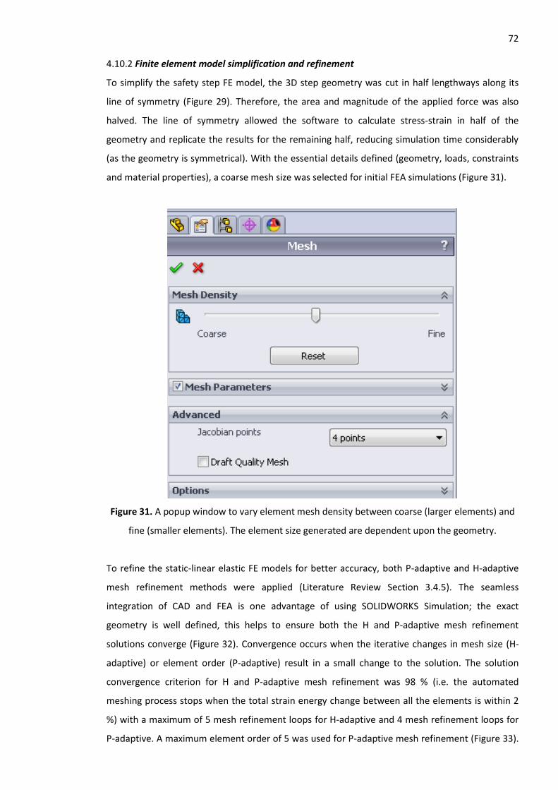
72 4.10.2 Finite element model simplification and refinement

To simplify the safety step FE model, the 3D step geometry was cut in half lengthways along its

line of symmetry (Figure 29). Therefore, the area and magnitude of the applied force was also

halved. The line of symmetry allowed the software to calculate stress-strain in half of the

geometry and replicate the results for the remaining half, reducing simulation time considerably

(as the geometry is symmetrical). With the essential details defined (geometry, loads, constraints

and material properties), a coarse mesh size was selected for initial FEA simulations (Figure 31).

Figure 31. A popup window to vary element mesh density between coarse (larger elements) and

fine (smaller elements). The element size generated are dependent upon the geometry.

To refine the static-linear elastic FE models for better accuracy, both P-adaptive and H-adaptive

mesh refinement methods were applied (Literature Review Section 3.4.5). The seamless

integration of CAD and FEA is one advantage of using SOLIDWORKS Simulation; the exact

geometry is well defined, this helps to ensure both the H and P-adaptive mesh refinement

solutions converge (Figure 32). Convergence occurs when the iterative changes in mesh size (H-

adaptive) or element order (P-adaptive) result in a small change to the solution. The solution

convergence criterion for H and P-adaptive mesh refinement was 98 % (i.e. the automated

meshing process stops when the total strain energy change between all the elements is within 2

%) with a maximum of 5 mesh refinement loops for H-adaptive and 4 mesh refinement loops for

P-adaptive. A maximum element order of 5 was used for P-adaptive mesh refinement (Figure 33).

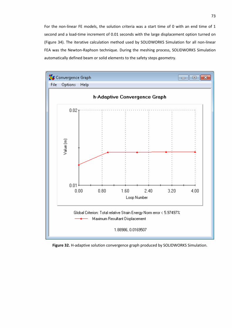
73 For the non-linear FE models, the solution criteria was a start time of 0 with an end time of 1

second and a load-time increment of 0.01 seconds with the large displacement option turned on

(Figure 34). The iterative calculation method used by SOLIDWORKS Simulation for all non-linear

FEA was the Newton-Raphson technique. During the meshing process, SOLIDWORKS Simulation

automatically defined beam or solid elements to the safety steps geometry.

Figure 32. H-adaptive solution convergence graph produced by SOLIDWORKS Simulation.

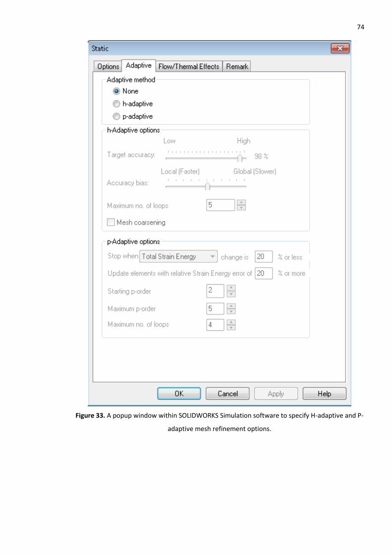
74

Figure 33. A popup window within SOLIDWORKS Simulation software to specify H-adaptive and P-

adaptive mesh refinement options.

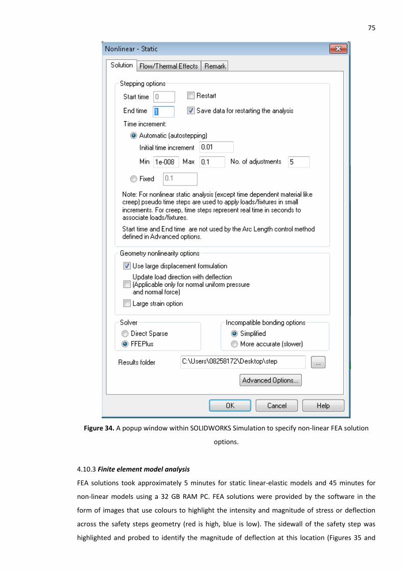
75

Figure 34. A popup window within SOLIDWORKS Simulation to specify non-linear FEA solution

options.

4.10.3 Finite element model analysis

FEA solutions took approximately 5 minutes for static linear-elastic models and 45 minutes for

non-linear models using a 32 GB RAM PC. FEA solutions were provided by the software in the

form of images that use colours to highlight the intensity and magnitude of stress or deflection

across the safety steps geometry (red is high, blue is low). The sidewall of the safety step was

highlighted and probed to identify the magnitude of deflection at this location (Figures 35 and

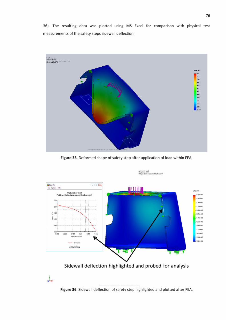
76 36). The resulting data was plotted using MS Excel for comparison with physical test

measurements of the safety steps sidewall deflection.

Figure 35. Deformed shape of safety step after application of load within FEA.

Figure 36. Sidewall deflection of safety step highlighted and plotted after FEA.

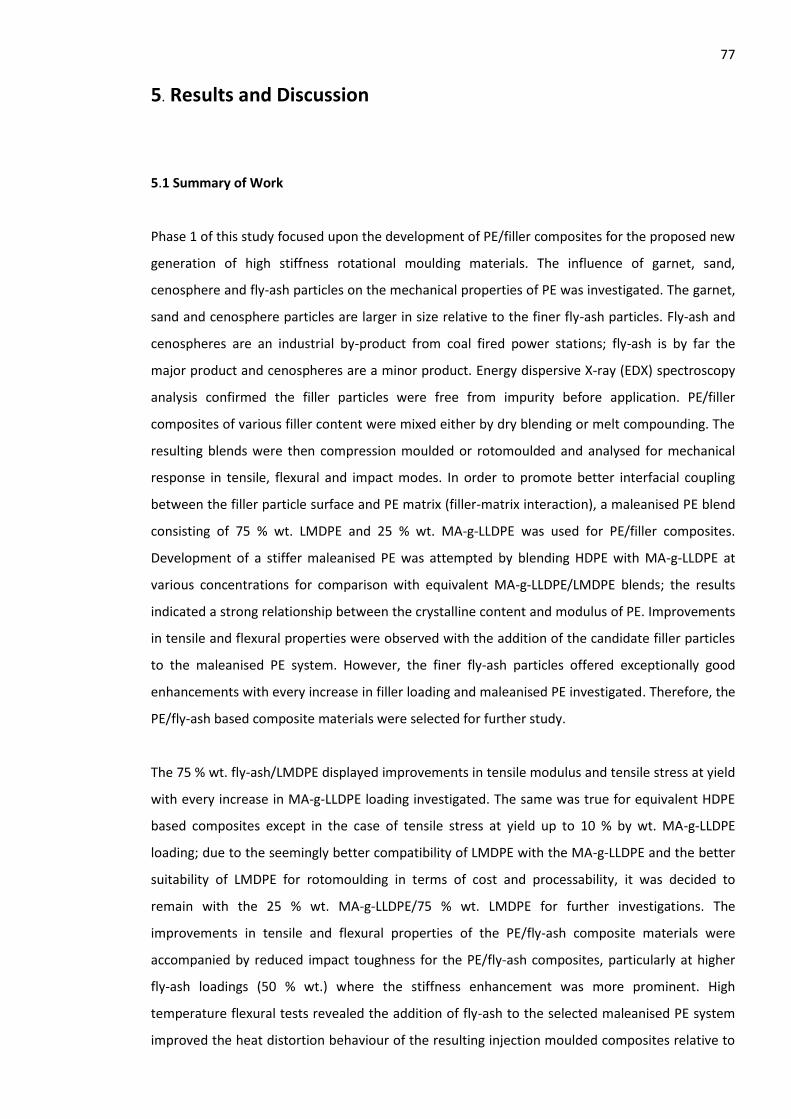
77

5. Results and Discussion

5.1 Summary of Work

Phase 1 of this study focused upon the development of PE/filler composites for the proposed new

generation of high stiffness rotational moulding materials. The influence of garnet, sand,

cenosphere and fly-ash particles on the mechanical properties of PE was investigated. The garnet,

sand and cenosphere particles are larger in size relative to the finer fly-ash particles. Fly-ash and

cenospheres are an industrial by-product from coal fired power stations; fly-ash is by far the

major product and cenospheres are a minor product. Energy dispersive X-ray (EDX) spectroscopy

analysis confirmed the filler particles were free from impurity before application. PE/filler

composites of various filler content were mixed either by dry blending or melt compounding. The

resulting blends were then compression moulded or rotomoulded and analysed for mechanical

response in tensile, flexural and impact modes. In order to promote better interfacial coupling

between the filler particle surface and PE matrix (filler-matrix interaction), a maleanised PE blend

consisting of 75 % wt. LMDPE and 25 % wt. MA-g-LLDPE was used for PE/filler composites.

Development of a stiffer maleanised PE was attempted by blending HDPE with MA-g-LLDPE at

various concentrations for comparison with equivalent MA-g-LLDPE/LMDPE blends; the results

indicated a strong relationship between the crystalline content and modulus of PE. Improvements

in tensile and flexural properties were observed with the addition of the candidate filler particles

to the maleanised PE system. However, the finer fly-ash particles offered exceptionally good

enhancements with every increase in filler loading and maleanised PE investigated. Therefore, the

PE/fly-ash based composite materials were selected for further study.

The 75 % wt. fly-ash/LMDPE displayed improvements in tensile modulus and tensile stress at yield

with every increase in MA-g-LLDPE loading investigated. The same was true for equivalent HDPE

based composites except in the case of tensile stress at yield up to 10 % by wt. MA-g-LLDPE

loading; due to the seemingly better compatibility of LMDPE with the MA-g-LLDPE and the better

suitability of LMDPE for rotomoulding in terms of cost and processability, it was decided to

remain with the 25 % wt. MA-g-LLDPE/75 % wt. LMDPE for further investigations. The

improvements in tensile and flexural properties of the PE/fly-ash composite materials were

accompanied by reduced impact toughness for the PE/fly-ash composites, particularly at higher

fly-ash loadings (50 % wt.) where the stiffness enhancement was more prominent. High

temperature flexural tests revealed the addition of fly-ash to the selected maleanised PE system

improved the heat distortion behaviour of the resulting injection moulded composites relative to

78 the unfilled matrix. TSE melt blended PE/fly-ash composites were rotomoulded into safety steps

and compression tested for comparison with unfilled PE safety steps. Tensile tests using

specimens cut from flat surfaces of the safety steps were also conducted and compared with

compression moulded equivalents. Only the 50 % wt. fly-ash PE composites offered stiffness

comparable to that of higher density rotomoulding PE grades. However, pinholes on the surfaces

of rotomoulded PE/fly-ash box test mouldings were evident with the increase in fly-ash; the latter

confirmed the challenge in moulding such highly filled PE using the zero-shear RM process. On the

other hand, it was seen that the variation in wall thickness of the rotomoulded PE safety steps

decreased with the addition of fly-ash; the increased melt viscosity may have allowed for better

dispersion of the melt during rotomoulding.

Phase 2 of this study focused upon developing a numerical database of material properties

required for computer simulation of the compression tests conducted on rotomoulded PE/fly-ash

composite safety steps. FEA was used to approximate the sidewall deflection of the safety steps

for comparison with actual sidewall deflection measurements. This exercise also served as a

method of identifying the numerical material parameters required for FEA of the new high

stiffness PE/fly-ash composite material; it was found that the tensile modulus, stress at yield,

Poisson’s ratio and tensile stress-strain response play an influential role in the outcome of FEA.

Furthermore, the geometry of the structure, mesh quality and boundary conditions of the FE

model (e.g. loads or constraints) are critical to the accuracy of FEA. With the parameters for FEA

identified, physical tests were conducted on rotomoulded PE/fly-ash materials and the

corresponding data was applied within FEA software; the resulting approximations of sidewall

deflection coincided reasonably well with physical measurements (depending on the analysis

type, mesh and material data of the FE model), confirming the practical value of the numerical

material data. However, in some instances significant differences between FEA and the actual

safety step are probably due to the effect of various complex factors such as the non-linear

behaviour of PE and the variation in wall thickness of rotomoulded parts. These differences

between FE model assumptions and physical rotomoulded parts arguably contribute to the

accuracy of FEA, exemplifying the importance of properly understanding the FEM for

rotomoulded parts.

During this study, both the tensile and flexural properties of the test materials were determined.

It was seen that the tensile properties of all PE/filler composites coincided well with the flexural

properties. In order to rationalise the volume of data discussed in this thesis, it was decided that

in the majority of cases only the tensile properties of PE/filler composites will be discussed, along

with a selection of other important data such as MFR and Charpy impact properties.

79 5.2 Characterisation of Materials for Composite Development

5.2.1 Effect of polymer structure

The principal PE matrix used in this investigation comprised of a blend of MA-g-LLDPE (25 % wt.)

with LMDPE; the presence of the MA coupling additive warrants the description “maleanised PE”.

For composites manufactured without the MA-g-LLDPE coupling additive, the matrix comprised of

a blend of 25 % wt. LLDPE (without MA grafting) with 75 % wt. LMDPE; the latter is described as

“analogue PE”. MA-g-LLDPE was introduced to improve filler-matrix interaction; the level of MA-g-

LLDPE selected was experimentally determined by the industrial partner for the large particle

composite application concerned, where the composites were made using a dry blending

approach. The melt flow rate (MFR) of both the maleanised and non maleanised PE is displayed

within Table 5 below, both of which the industrial sponsor Rotomotive Ltd. confirmed to be

suitable for rotomoulding by previous investigation. The difference in MFR between both the

maleanised and non-maleanised PE grades was negligible, indicating the introduction of maleic

anhydride to PE (in this instance) has no real impact on the MFR. However, it was appreciated

that the addition of fly-ash particles to PE does have a negative impact on the MFR (Section 5.8).

Table 5. Melt flow rate of maleanised and analogue PE used in this work.

Melt Flow Rate

Maleanised PE Standard Deviation

Analogue PE Standard Deviation

dg min-1 3.424 0.025 3.415 0.014

5.2.2 Dual polyethylene blends

5.2.2.1 Dry blended formulations

Dry blending MA-g-LLDPE with HDPE (replacing LMDPE) was conducted in an attempt to further

improve the mechanical properties of the base PE used for composites in this work. Differential

Scanning Calorimetry (DSC) data indicated HDPE and LMDPE are inherently of higher crystallinity

than MA-g-LLDPE (with HDPE having the highest crystalline content). When combined with MA-g-

LLDPE their % crystallinity progressively decreases; these crystalline regions are effectively the

mechanical reinforcing phases of PE. Figures 37-39 display graphs of results (note that in some

instances the error bars appear absent as they were smaller than the plot symbols). Tables

containing standard deviation data for tensile parameters found in this investigation are available

within the Appendix Section 3. The relevant Appendix table number is provided in the figure

caption. A compilation of all DSC data is provided in Appendix Section 4. Table 6 identifies the

various concentrations of HDPE or LMDPE with MA-g-LLDPE; eight replicate samples of each blend

combination were tested, five of the most consistent values were selected and averaged.

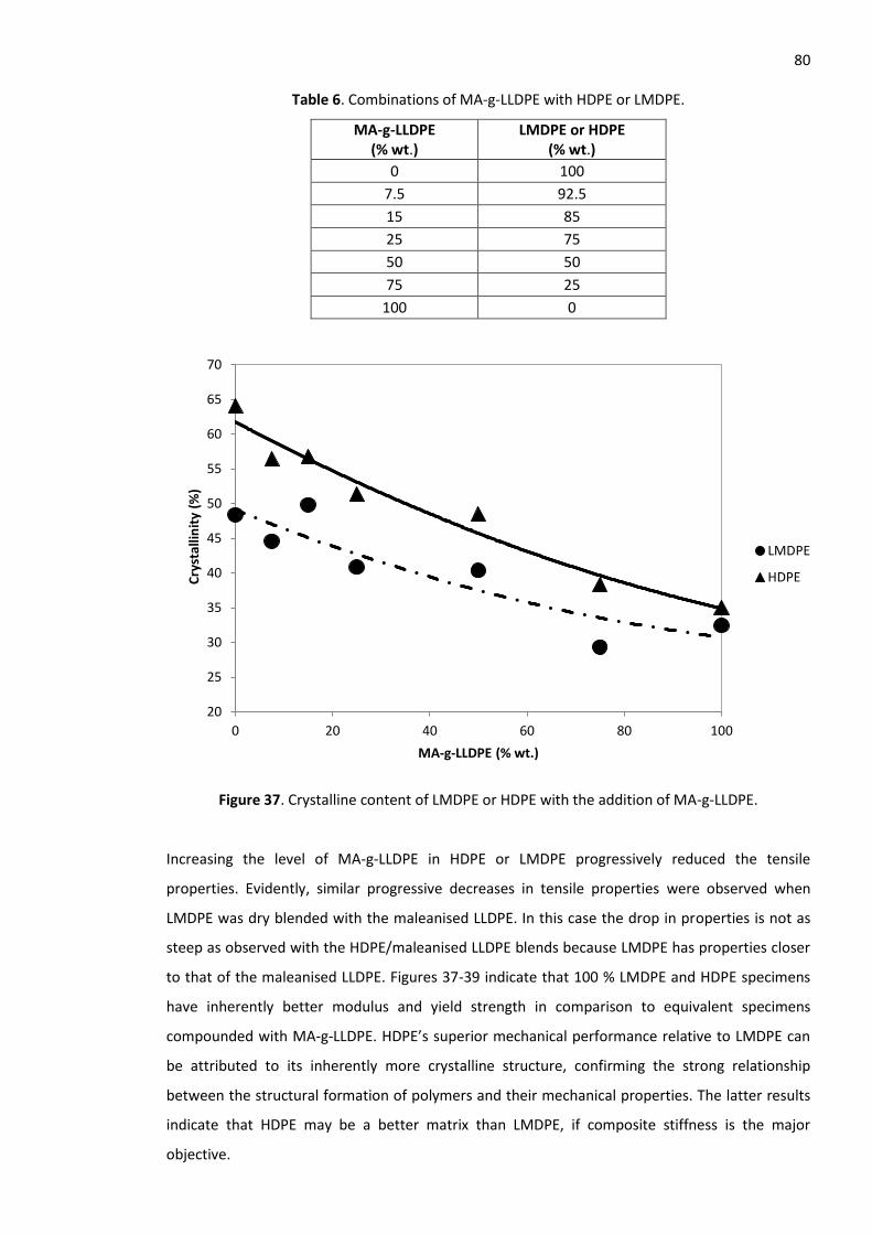
80

Table 6. Combinations of MA-g-LLDPE with HDPE or LMDPE.

MA-g-LLDPE (% wt.)

LMDPE or HDPE (% wt.)

0 100

7.5 92.5

15 85

25 75

50 50

75 25

100 0

Figure 37. Crystalline content of LMDPE or HDPE with the addition of MA-g-LLDPE.

Increasing the level of MA-g-LLDPE in HDPE or LMDPE progressively reduced the tensile

properties. Evidently, similar progressive decreases in tensile properties were observed when

LMDPE was dry blended with the maleanised LLDPE. In this case the drop in properties is not as

steep as observed with the HDPE/maleanised LLDPE blends because LMDPE has properties closer

to that of the maleanised LLDPE. Figures 37-39 indicate that 100 % LMDPE and HDPE specimens

have inherently better modulus and yield strength in comparison to equivalent specimens

compounded with MA-g-LLDPE. HDPE’s superior mechanical performance relative to LMDPE can

be attributed to its inherently more crystalline structure, confirming the strong relationship

between the structural formation of polymers and their mechanical properties. The latter results

indicate that HDPE may be a better matrix than LMDPE, if composite stiffness is the major

objective.

20

25

30

35

40

45

50

55

60

65

70

0 20 40 60 80 100

Cry

stal

linit

y (%

)

MA-g-LLDPE (% wt.)

LMDPE

HDPE

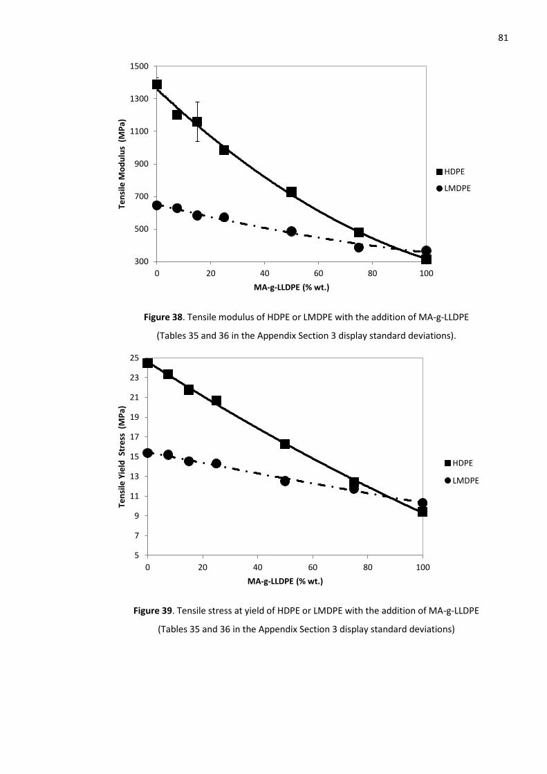
81

Figure 38. Tensile modulus of HDPE or LMDPE with the addition of MA-g-LLDPE

(Tables 35 and 36 in the Appendix Section 3 display standard deviations).

Figure 39. Tensile stress at yield of HDPE or LMDPE with the addition of MA-g-LLDPE

(Tables 35 and 36 in the Appendix Section 3 display standard deviations)

300

500

700

900

1100

1300

1500

0 20 40 60 80 100

Ten

sile

Mo

du

lus

(M

Pa)

MA-g-LLDPE (% wt.)

HDPE

LMDPE

5

7

9

11

13

15

17

19

21

23

25

0 20 40 60 80 100

Ten

sile

Yie

ld S

tre

ss (

MP

a)

MA-g-LLDPE (% wt.)

HDPE

LMDPE

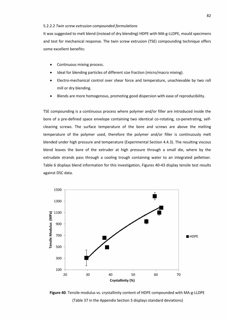
82 5.2.2.2 Twin screw extrusion compounded formulations

It was suggested to melt blend (instead of dry blending) HDPE with MA-g-LLDPE, mould specimens

and test for mechanical response. The twin screw extrusion (TSE) compounding technique offers

some excellent benefits:

Continuous mixing process.

Ideal for blending particles of different size fraction (micro/macro mixing).

Electro-mechanical control over shear force and temperature, unachievable by two roll

mill or dry blending.

Blends are more homogenous, promoting good dispersion with ease of reproducibility.

TSE compounding is a continuous process where polymer and/or filler are introduced inside the

bore of a pre-defined space envelope containing two identical co-rotating, co-penetrating, self-

cleaning screws. The surface temperature of the bore and screws are above the melting

temperature of the polymer used, therefore the polymer and/or filler is continuously melt

blended under high pressure and temperature (Experimental Section 4.4.3). The resulting viscous

blend leaves the bore of the extruder at high pressure through a small die, where by the

extrudate strands pass through a cooling trough containing water to an integrated pelletiser.

Table 6 displays blend information for this investigation, Figures 40-43 display tensile test results

against DSC data.

Figure 40. Tensile modulus vs. crystallinity content of HDPE compounded with MA-g-LLDPE

(Table 37 in the Appendix Section 3 displays standard deviations)

100

300

500

700

900

1100

1300

1500

20 30 40 50 60 70

Ten

sile

Mo

du

lus

(M

Pa)

Crystallinity (%)

HDPE

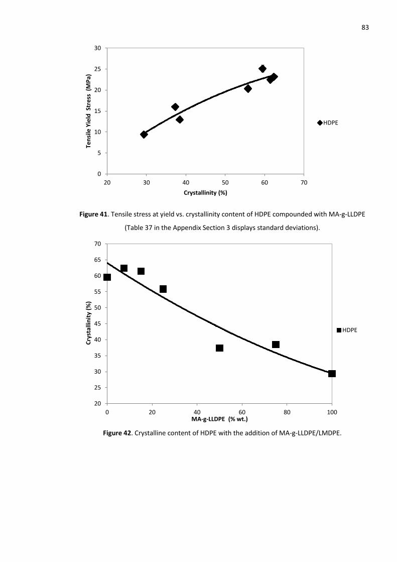
83

Figure 41. Tensile stress at yield vs. crystallinity content of HDPE compounded with MA-g-LLDPE

(Table 37 in the Appendix Section 3 displays standard deviations).

Figure 42. Crystalline content of HDPE with the addition of MA-g-LLDPE/LMDPE.

0

5

10

15

20

25

30

20 30 40 50 60 70

Ten

sile

Yie

ld S

tre

ss (

MP

a)

Crystallinity (%)

HDPE

20

25

30

35

40

45

50

55

60

65

70

0 20 40 60 80 100

Cry

stal

linit

y (%

)

MA-g-LLDPE (% wt.)

HDPE

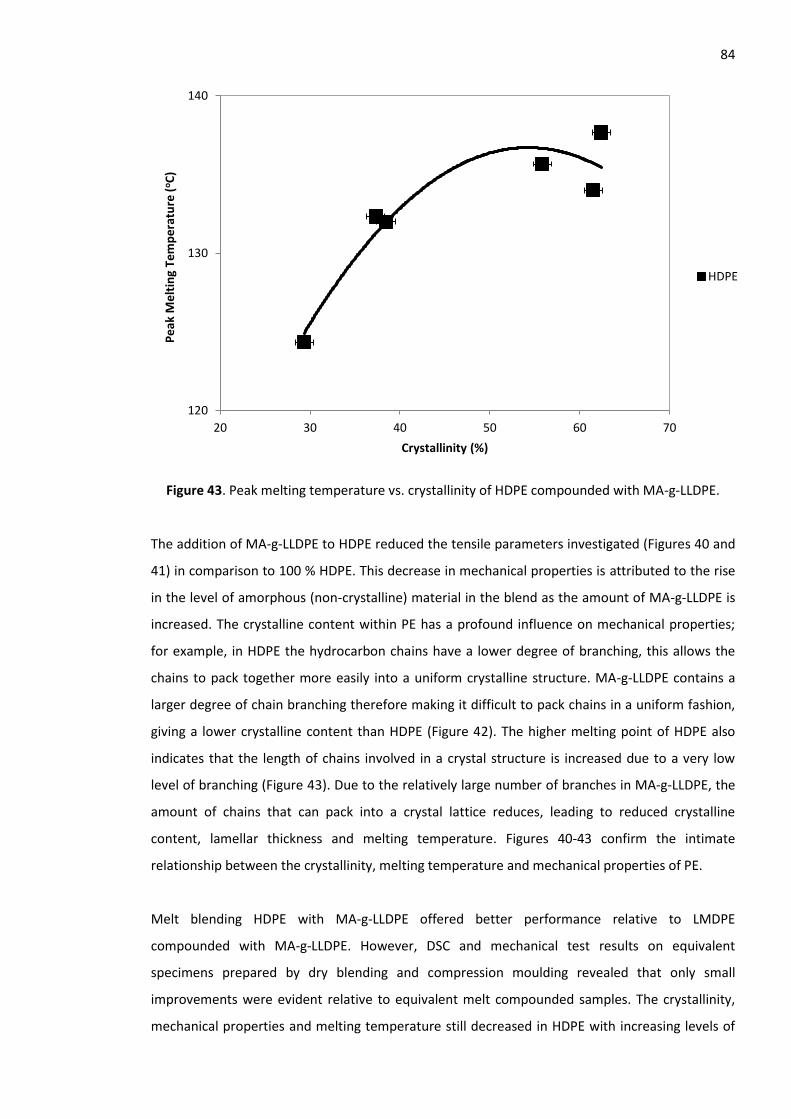
84

Figure 43. Peak melting temperature vs. crystallinity of HDPE compounded with MA-g-LLDPE.

The addition of MA-g-LLDPE to HDPE reduced the tensile parameters investigated (Figures 40 and

41) in comparison to 100 % HDPE. This decrease in mechanical properties is attributed to the rise

in the level of amorphous (non-crystalline) material in the blend as the amount of MA-g-LLDPE is

increased. The crystalline content within PE has a profound influence on mechanical properties;

for example, in HDPE the hydrocarbon chains have a lower degree of branching, this allows the

chains to pack together more easily into a uniform crystalline structure. MA-g-LLDPE contains a

larger degree of chain branching therefore making it difficult to pack chains in a uniform fashion,

giving a lower crystalline content than HDPE (Figure 42). The higher melting point of HDPE also

indicates that the length of chains involved in a crystal structure is increased due to a very low

level of branching (Figure 43). Due to the relatively large number of branches in MA-g-LLDPE, the

amount of chains that can pack into a crystal lattice reduces, leading to reduced crystalline

content, lamellar thickness and melting temperature. Figures 40-43 confirm the intimate

relationship between the crystallinity, melting temperature and mechanical properties of PE.

Melt blending HDPE with MA-g-LLDPE offered better performance relative to LMDPE

compounded with MA-g-LLDPE. However, DSC and mechanical test results on equivalent

specimens prepared by dry blending and compression moulding revealed that only small

improvements were evident relative to equivalent melt compounded samples. The crystallinity,

mechanical properties and melting temperature still decreased in HDPE with increasing levels of

120

130

140

20 30 40 50 60 70

Pe

ak M

elt

ing

Tem

pe

ratu

re (

oC

)

Crystallinity (%)

HDPE

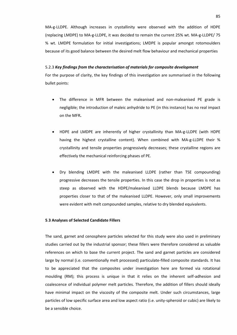
85 MA-g-LLDPE. Although increases in crystallinity were observed with the addition of HDPE

(replacing LMDPE) to MA-g-LLDPE, it was decided to remain the current 25% wt. MA-g-LLDPE/ 75

% wt. LMDPE formulation for initial investigations; LMDPE is popular amongst rotomoulders

because of its good balance between the desired melt flow behaviour and mechanical properties

5.2.3 Key findings from the characterisation of materials for composite development

For the purpose of clarity, the key findings of this investigation are summarised in the following

bullet points:

The difference in MFR between the maleanised and non-maleanised PE grade is

negligible; the introduction of maleic anhydride to PE (in this instance) has no real impact

on the MFR.

HDPE and LMDPE are inherently of higher crystallinity than MA-g-LLDPE (with HDPE

having the highest crystalline content). When combined with MA-g-LLDPE their %

crystallinity and tensile properties progressively decreases; these crystalline regions are

effectively the mechanical reinforcing phases of PE.

Dry blending LMDPE with the maleanised LLDPE (rather than TSE compounding)

progressive decreases the tensile properties. In this case the drop in properties is not as

steep as observed with the HDPE/maleanised LLDPE blends because LMDPE has

properties closer to that of the maleanised LLDPE. However, only small improvements

were evident with melt compounded samples, relative to dry blended equivalents.

5.3 Analyses of Selected Candidate Fillers

The sand, garnet and cenosphere particles selected for this study were also used in preliminary

studies carried out by the industrial sponsor; these fillers were therefore considered as valuable

references on which to base the current project. The sand and garnet particles are considered

large by normal (i.e. conventionally melt processed) particulate-filled composite standards. It has

to be appreciated that the composites under investigation here are formed via rotational

moulding (RM); this process is unique in that it relies on the inherent self-adhesion and

coalescence of individual polymer melt particles. Therefore, the addition of fillers should ideally

have minimal impact on the viscosity of the composite melt. Under such circumstances, large

particles of low specific surface area and low aspect ratio (i.e. unity-spheroid or cubic) are likely to

be a sensible choice.

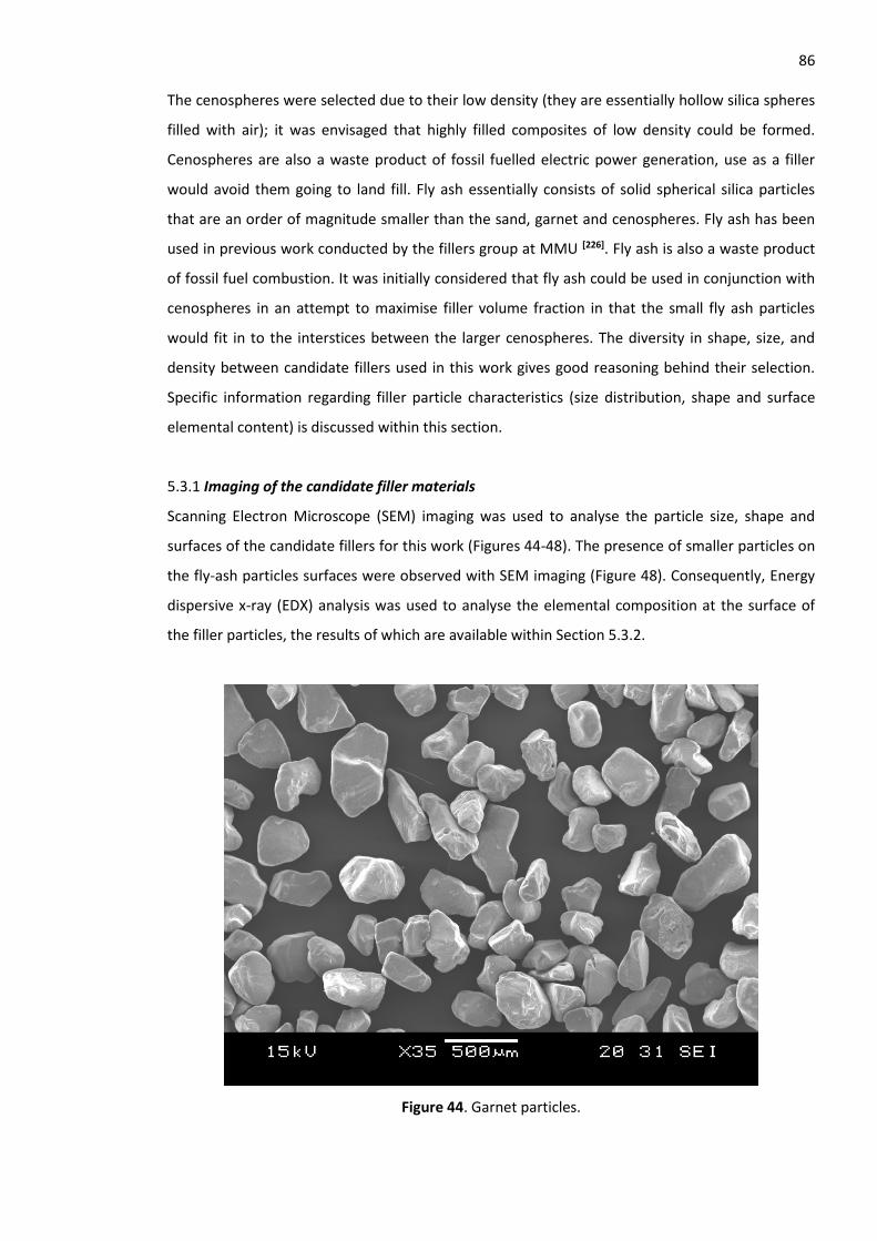
86 The cenospheres were selected due to their low density (they are essentially hollow silica spheres

filled with air); it was envisaged that highly filled composites of low density could be formed.

Cenospheres are also a waste product of fossil fuelled electric power generation, use as a filler

would avoid them going to land fill. Fly ash essentially consists of solid spherical silica particles

that are an order of magnitude smaller than the sand, garnet and cenospheres. Fly ash has been

used in previous work conducted by the fillers group at MMU [226]. Fly ash is also a waste product

of fossil fuel combustion. It was initially considered that fly ash could be used in conjunction with

cenospheres in an attempt to maximise filler volume fraction in that the small fly ash particles

would fit in to the interstices between the larger cenospheres. The diversity in shape, size, and

density between candidate fillers used in this work gives good reasoning behind their selection.

Specific information regarding filler particle characteristics (size distribution, shape and surface

elemental content) is discussed within this section.

5.3.1 Imaging of the candidate filler materials

Scanning Electron Microscope (SEM) imaging was used to analyse the particle size, shape and

surfaces of the candidate fillers for this work (Figures 44-48). The presence of smaller particles on

the fly-ash particles surfaces were observed with SEM imaging (Figure 48). Consequently, Energy

dispersive x-ray (EDX) analysis was used to analyse the elemental composition at the surface of

the filler particles, the results of which are available within Section 5.3.2.

Figure 44. Garnet particles.

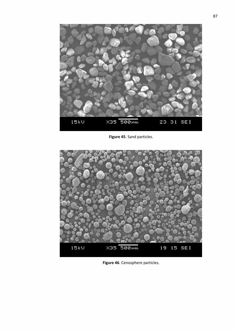
87

Figure 45. Sand particles.

Figure 46. Cenosphere particles.

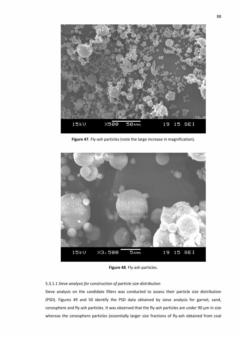
88

Figure 47. Fly-ash particles (note the large increase in magnification).

Figure 48. Fly-ash particles.

5.3.1.1 Sieve analysis for construction of particle size distribution

Sieve analysis on the candidate fillers was conducted to assess their particle size distribution

(PSD). Figures 49 and 50 identify the PSD data obtained by sieve analysis for garnet, sand,

cenosphere and fly-ash particles. It was observed that the fly-ash particles are under 90 µm in size

whereas the cenosphere particles (essentially larger size fractions of fly-ash obtained from coal

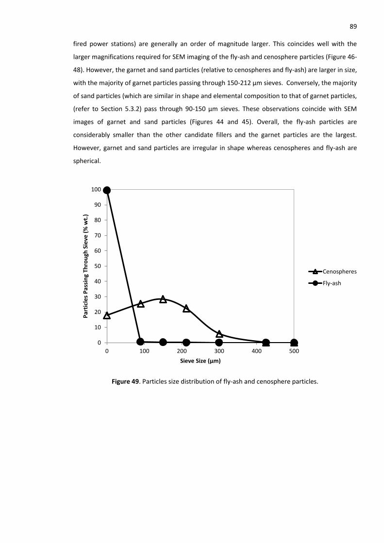
89 fired power stations) are generally an order of magnitude larger. This coincides well with the

larger magnifications required for SEM imaging of the fly-ash and cenosphere particles (Figure 46-

48). However, the garnet and sand particles (relative to cenospheres and fly-ash) are larger in size,

with the majority of garnet particles passing through 150-212 µm sieves. Conversely, the majority

of sand particles (which are similar in shape and elemental composition to that of garnet particles,

(refer to Section 5.3.2) pass through 90-150 µm sieves. These observations coincide with SEM

images of garnet and sand particles (Figures 44 and 45). Overall, the fly-ash particles are

considerably smaller than the other candidate fillers and the garnet particles are the largest.

However, garnet and sand particles are irregular in shape whereas cenospheres and fly-ash are

spherical.

Figure 49. Particles size distribution of fly-ash and cenosphere particles.

0

10

20

30

40

50

60

70

80

90

100

0 100 200 300 400 500

Par

ticl

es

Pas

sin

g Th

rou

gh S

ieve

(%

wt.

)

Sieve Size (µm)

Cenospheres

Fly-ash

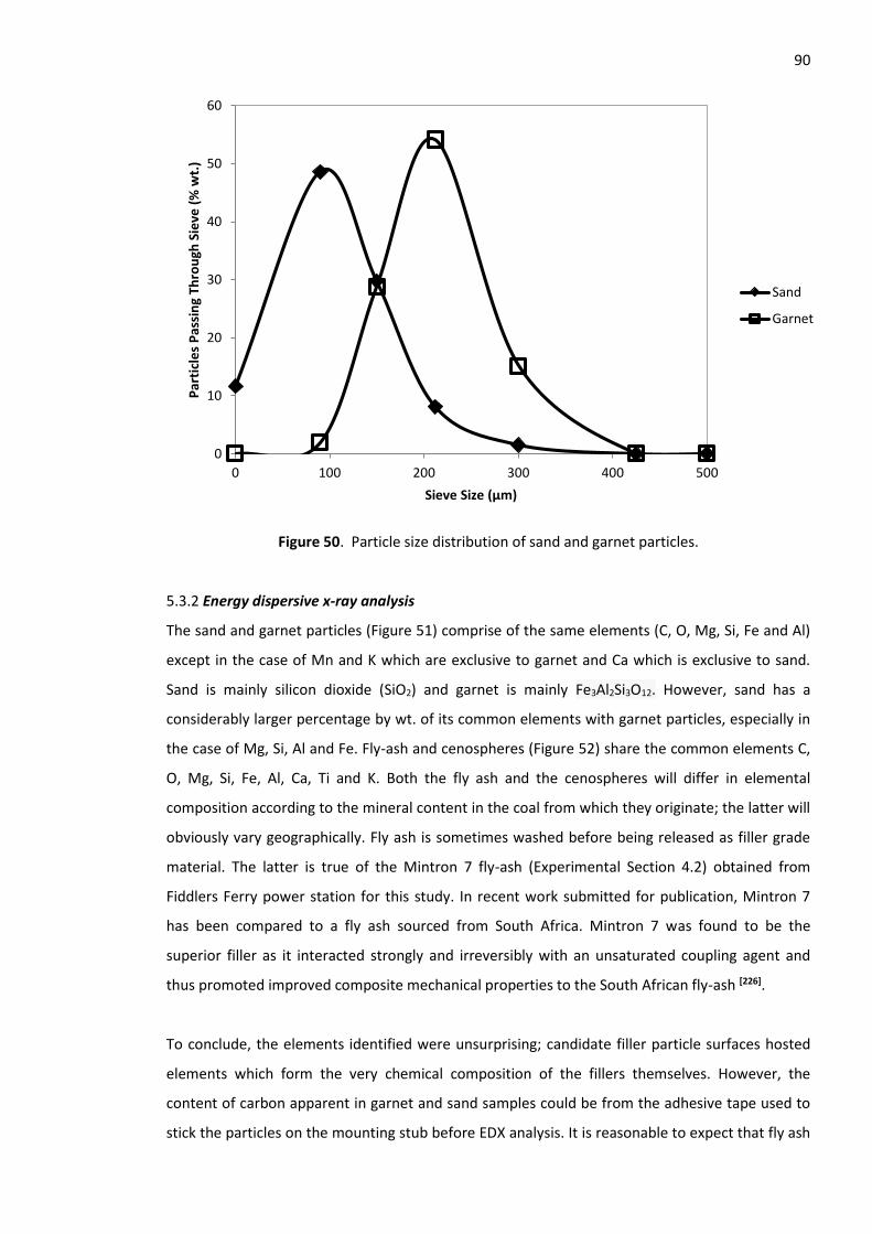
90

Figure 50. Particle size distribution of sand and garnet particles.

5.3.2 Energy dispersive x-ray analysis

The sand and garnet particles (Figure 51) comprise of the same elements (C, O, Mg, Si, Fe and Al)

except in the case of Mn and K which are exclusive to garnet and Ca which is exclusive to sand.

Sand is mainly silicon dioxide (SiO2) and garnet is mainly Fe3Al2Si3O12. However, sand has a

considerably larger percentage by wt. of its common elements with garnet particles, especially in

the case of Mg, Si, Al and Fe. Fly-ash and cenospheres (Figure 52) share the common elements C,

O, Mg, Si, Fe, Al, Ca, Ti and K. Both the fly ash and the cenospheres will differ in elemental

composition according to the mineral content in the coal from which they originate; the latter will

obviously vary geographically. Fly ash is sometimes washed before being released as filler grade

material. The latter is true of the Mintron 7 fly-ash (Experimental Section 4.2) obtained from

Fiddlers Ferry power station for this study. In recent work submitted for publication, Mintron 7

has been compared to a fly ash sourced from South Africa. Mintron 7 was found to be the

superior filler as it interacted strongly and irreversibly with an unsaturated coupling agent and

thus promoted improved composite mechanical properties to the South African fly-ash [226].

To conclude, the elements identified were unsurprising; candidate filler particle surfaces hosted

elements which form the very chemical composition of the fillers themselves. However, the

content of carbon apparent in garnet and sand samples could be from the adhesive tape used to

stick the particles on the mounting stub before EDX analysis. It is reasonable to expect that fly ash

0

10

20

30

40

50

60

0 100 200 300 400 500

Par

ticl

es

Pas

sin

g Th

rou

gh S

ieve

(%

wt.

)

Sieve Size (µm)

Sand

Garnet

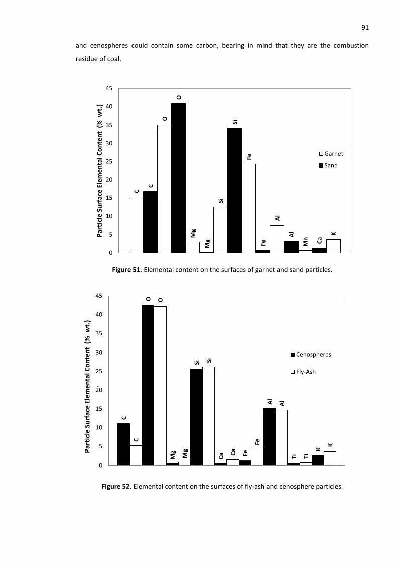
91 and cenospheres could contain some carbon, bearing in mind that they are the combustion

residue of coal.

Figure 51. Elemental content on the surfaces of garnet and sand particles.

Figure 52. Elemental content on the surfaces of fly-ash and cenosphere particles.

C

C

O

O

Mg

Mg

Si

Si

Fe

Fe

Al

Al

Mn Ca

K

0

5

10

15

20

25

30

35

40

45

Par

ticl

e Su

rfac

e El

eme

nta

l Co

nte

nt

(%

wt.

)

Garnet

Sand

C

C

O O

Mg

Mg

Si Si

Ca C

a

Fe

Fe

Al

Al

Ti Ti

K K

0

5

10

15

20

25

30

35

40

45

Par

ticl

e Su

rfac

e El

eme

nta

l Co

nte

nt

(%

wt.

).

Cenospheres

Fly-Ash

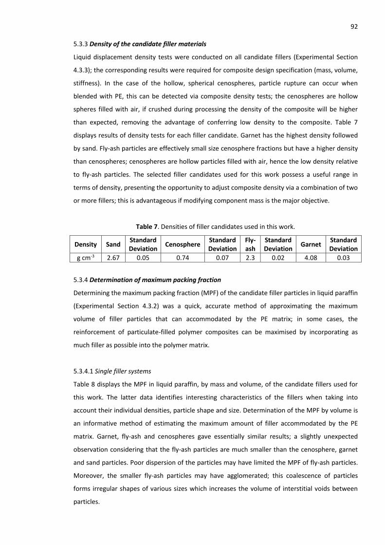
92 5.3.3 Density of the candidate filler materials

Liquid displacement density tests were conducted on all candidate fillers (Experimental Section

4.3.3); the corresponding results were required for composite design specification (mass, volume,

stiffness). In the case of the hollow, spherical cenospheres, particle rupture can occur when

blended with PE, this can be detected via composite density tests; the cenospheres are hollow

spheres filled with air, if crushed during processing the density of the composite will be higher

than expected, removing the advantage of conferring low density to the composite. Table 7

displays results of density tests for each filler candidate. Garnet has the highest density followed

by sand. Fly-ash particles are effectively small size cenosphere fractions but have a higher density

than cenospheres; cenospheres are hollow particles filled with air, hence the low density relative

to fly-ash particles. The selected filler candidates used for this work possess a useful range in

terms of density, presenting the opportunity to adjust composite density via a combination of two

or more fillers; this is advantageous if modifying component mass is the major objective.

Table 7. Densities of filler candidates used in this work.

Density Sand Standard Deviation

Cenosphere Standard Deviation

Fly-ash

Standard Deviation

Garnet Standard Deviation

g cm-3 2.67 0.05 0.74 0.07 2.3 0.02 4.08 0.03

5.3.4 Determination of maximum packing fraction

Determining the maximum packing fraction (MPF) of the candidate filler particles in liquid paraffin

(Experimental Section 4.3.2) was a quick, accurate method of approximating the maximum

volume of filler particles that can accommodated by the PE matrix; in some cases, the

reinforcement of particulate-filled polymer composites can be maximised by incorporating as

much filler as possible into the polymer matrix.

5.3.4.1 Single filler systems

Table 8 displays the MPF in liquid paraffin, by mass and volume, of the candidate fillers used for

this work. The latter data identifies interesting characteristics of the fillers when taking into

account their individual densities, particle shape and size. Determination of the MPF by volume is

an informative method of estimating the maximum amount of filler accommodated by the PE

matrix. Garnet, fly-ash and cenospheres gave essentially similar results; a slightly unexpected

observation considering that the fly-ash particles are much smaller than the cenosphere, garnet

and sand particles. Poor dispersion of the particles may have limited the MPF of fly-ash particles.

Moreover, the smaller fly-ash particles may have agglomerated; this coalescence of particles

forms irregular shapes of various sizes which increases the volume of interstitial voids between

particles.

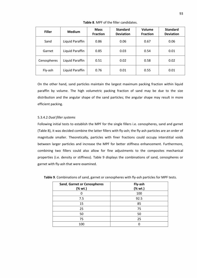
93

Table 8. MPF of the filler candidates.

Filler Medium Mass

Fraction Standard Deviation

Volume Fraction

Standard Deviation

Sand Liquid Paraffin 0.86 0.06 0.67 0.06

Garnet Liquid Paraffin 0.85 0.03 0.54 0.01

Cenospheres Liquid Paraffin 0.51 0.02 0.58 0.02

Fly-ash Liquid Paraffin 0.76 0.01 0.55 0.01

On the other hand, sand particles maintain the largest maximum packing fraction within liquid

paraffin by volume. The high volumetric packing fraction of sand may be due to the size

distribution and the angular shape of the sand particles; the angular shape may result in more

efficient packing.

5.3.4.2 Dual filler systems

Following initial tests to establish the MPF for the single fillers i.e. cenospheres, sand and garnet

(Table 8), it was decided combine the latter fillers with fly-ash; the fly-ash particles are an order of

magnitude smaller. Theoretically, particles with finer fractions could occupy interstitial voids

between larger particles and increase the MPF for better stiffness enhancement. Furthermore,

combining two fillers could also allow for fine adjustments to the composites mechanical

properties (i.e. density or stiffness). Table 9 displays the combinations of sand, cenospheres or

garnet with fly-ash that were examined.

Table 9. Combinations of sand, garnet or cenospheres with fly-ash particles for MPF tests.

Sand, Garnet or Cenospheres (% wt.)

Fly-ash (% wt.)

0 100

7.5 92.5

15 85

25 75

50 50

75 25

100 0

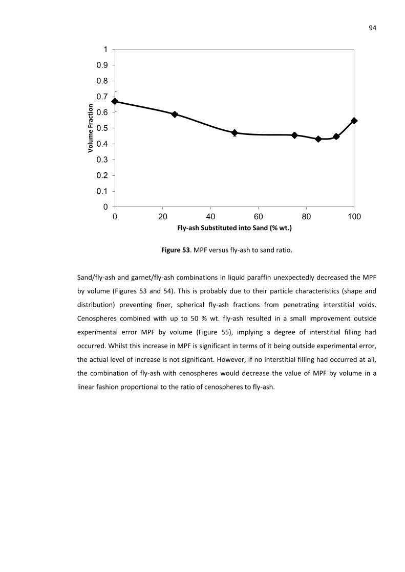
94

Figure 53. MPF versus fly-ash to sand ratio.

Sand/fly-ash and garnet/fly-ash combinations in liquid paraffin unexpectedly decreased the MPF

by volume (Figures 53 and 54). This is probably due to their particle characteristics (shape and

distribution) preventing finer, spherical fly-ash fractions from penetrating interstitial voids.

Cenospheres combined with up to 50 % wt. fly-ash resulted in a small improvement outside

experimental error MPF by volume (Figure 55), implying a degree of interstitial filling had

occurred. Whilst this increase in MPF is significant in terms of it being outside experimental error,

the actual level of increase is not significant. However, if no interstitial filling had occurred at all,

the combination of fly-ash with cenospheres would decrease the value of MPF by volume in a

linear fashion proportional to the ratio of cenospheres to fly-ash.

0

0.1

0.2

0.3

0.4

0.5

0.6

0.7

0.8

0.9

1

0 20 40 60 80 100

Vo

lum

e F

ract

ion

Fly-ash Substituted into Sand (% wt.)

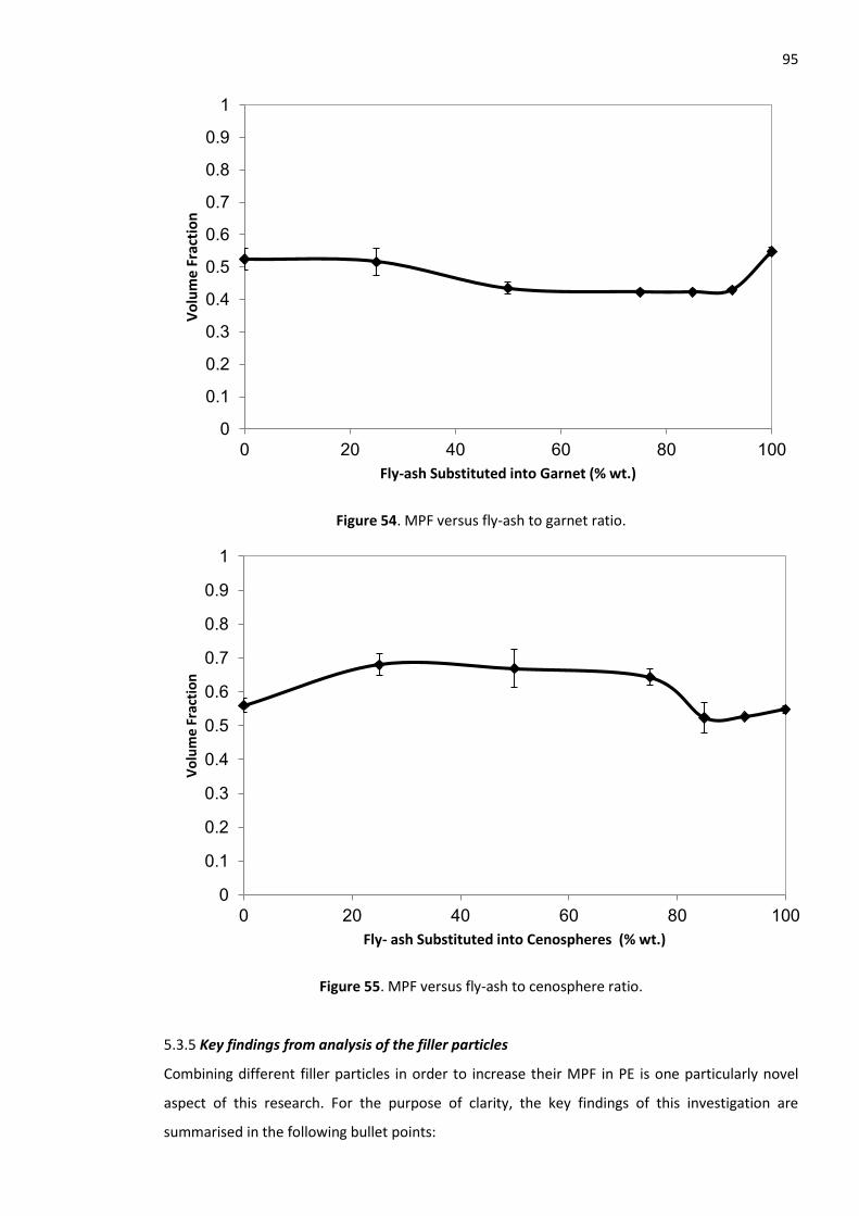
95

Figure 54. MPF versus fly-ash to garnet ratio.

Figure 55. MPF versus fly-ash to cenosphere ratio.

5.3.5 Key findings from analysis of the filler particles

Combining different filler particles in order to increase their MPF in PE is one particularly novel

aspect of this research. For the purpose of clarity, the key findings of this investigation are

summarised in the following bullet points:

0

0.1

0.2

0.3

0.4

0.5

0.6

0.7

0.8

0.9

1

0 20 40 60 80 100

Vo

lum

e F

ract

ion

Fly-ash Substituted into Garnet (% wt.)

0

0.1

0.2

0.3

0.4

0.5

0.6

0.7

0.8

0.9

1

0 20 40 60 80 100

Vo

lum

e F

ract

ion

Fly- ash Substituted into Cenospheres (% wt.)

96

The fly-ash particles are under 90 µm in size whereas the cenosphere particles are

generally an order of magnitude larger. However, the garnet and sand particles (relative

to cenospheres and fly-ash) are larger in size, with the majority of garnet particles passing

through 150-212 µm sieves. Conversely, the majority of sand particles (which are similar

in shape and elemental composition to that of garnet particles), pass through 90-150 µm

sieves.

Garnet and sand particles are irregular in shape whereas cenospheres and fly-ash are

spherical.

The sand and garnet particles comprise of the same elements (C, O, Mg, Si, Fe and Al)

except in the case of Mn and K which are exclusive to garnet and Ca which is exclusive to

sand. Sand is mainly silicon dioxide (SiO2) and garnet is mainly Fe3Al2Si3O12. However, sand

has a considerably larger percentage by wt. of its common elements with garnet particles,

especially in the case of Mg, Si, Al and Fe.

Fly-ash and cenospheres share the common elements C, O, Mg, Si, Fe, Al, Ca, Ti and K.

Both the fly ash and the cenospheres will differ in elemental composition according to the

mineral content in the coal from which they originate; the latter will vary geographically.

Garnet, fly-ash and cenospheres have essentially similar MPF results; a slightly

unexpected observation considering that the fly-ash particles are much smaller than the

cenosphere, garnet and sand particles. Poor dispersion of the particles may have limited

the MPF of fly-ash particles. Moreover, the smaller fly-ash particles may have

agglomerated; this coalescence of particles forms irregular shapes of various sizes which

increases the volume of interstitial voids between particles.

The sand particles maintain the largest maximum packing fraction within liquid paraffin by

volume. The high volumetric packing fraction of sand may be due to the size distribution

and the angular shape of the sand particles; the angular shape may result in more

efficient packing.

Sand/fly-ash and garnet/fly-ash combinations in liquid paraffin unexpectedly decreased

the MPF by volume. This is probably due to their particle characteristics (shape and

distribution) preventing finer, spherical fly-ash fractions from penetrating interstitial

voids.

97

Cenospheres combined with up to 50 % wt. fly-ash resulted in a small improvement

outside experimental error MPF by volume (Figure 55), implying a degree of interstitial

filling had occurred. Whilst this increase in MPF is significant in terms of it being outside

experimental error, the actual level of increase is not significant.

5.4 Comparison of Composite Formation Processes for Large Particle Composites (Dry Blending

of Pre-Mix versus Two Roll Mill Melt Blending and Moulding)

The initial PE/filler composites were dry blended in the bowl of a Brevel Model SMH2 domestic

planetary mixer before moulding. Dry blending was the quickest method of mixing materials for

compression moulding; the relatively short production time for dry blended PE/filler composites

provided the opportunity to establish firm test protocols quickly. The dry blending approach was

also successfully used by the industrial sponsor Rotomotive Ltd. for the large particle application

concerned. Therefore, a database of properties was available to compare with the data found in

this study. However, it was appreciated that uniform filler particle dispersion quality and sufficient

matrix-filler interaction may not be achievable via dry blending and compression moulding;

particle dispersion quality and the strength of filler-matrix interaction have a significant effect on

the mechanical properties of PE/filler composites. Therefore, a melt blend route was attempted

using a two roll mill; the latter method offered the following benefits:

Both rolls are above the melting temperature (Tm) of PE, physically incorporating the filler

particles by shear within a liquid PE matrix.

The separation and relative rotational speed of individual rolls can be varied by the

operator; this allows the level of shear to be precisely tailored.

Better filler-matrix interaction; the filler particle surface is more intimately wetted by a

sheared polymer melt.

Table 10. Blend details of two roll milled and dry blended composites.

MA-g-LLDPE/LMDPE (% wt.)

Filler (% wt.)

100 0

75 25

50 50

40 60

30 70

25 75

20 80

15 85

98 To assess the effect of blending method on the mechanical properties of PE/filler composites

(Table 10), the tensile properties of dry blended PE/filler prepared composites were analysed in

comparison to equivalent two roll mill prepared specimens (Figures 56-59). The dry blended

PE/cenosphere composites at filler loadings above 60 % wt. were difficult to process thus

rendering them brittle and unsuitable for testing. A CNC water jet cutter (operating to a tolerance

of ± 0.1mm) was used to cut flexural and tensile test pieces from composites produced by

compression moulding at MMU; these composites were prepared by pre-blending the filler and

PE matrix in the melt state using a two roll mill. However, the test materials produced at

Rotomotive Ltd. by dry blending the filler with PE and compression moulding were die stamped.

The die stamping method was reasonable for the unfilled matrix and the more lightly filled

composites, although as filler content increased it became evident that the edges of the test

pieces were damaged via this method (manifested as stress whitening). Water jet cutting was a

superior method for the production of test pieces relative to die stamping; the edges of even the

highly filled composite test pieces were clean with no stress whitening evident. There is obvious

potential for the two different test piece preparation methods to confound differences in

properties between the composites prepared by melt blending and those prepared by dry

blending. It can nevertheless be said with some confidence that composite stiffness will not be

affected by the test piece preparation method, as the samples are not stressed to failure during

such examination. Due to the presence of defects at the edges of the die stamped samples, it is

reasonable to expect them to fail prematurely. Therefore, it can be argued that the ultimate

properties (tensile strength and tensile stress at yield) cannot be compared with those composites

prepared by water jet cutting. Despite this argument it appears that the superiority of dry

blending for production of composites based on larger particles (particularly garnet and to a lesser

extent sand) in terms of tensile yield strength is still observable, regardless of the fact the dry

blended samples were die stamped (Figure 58).

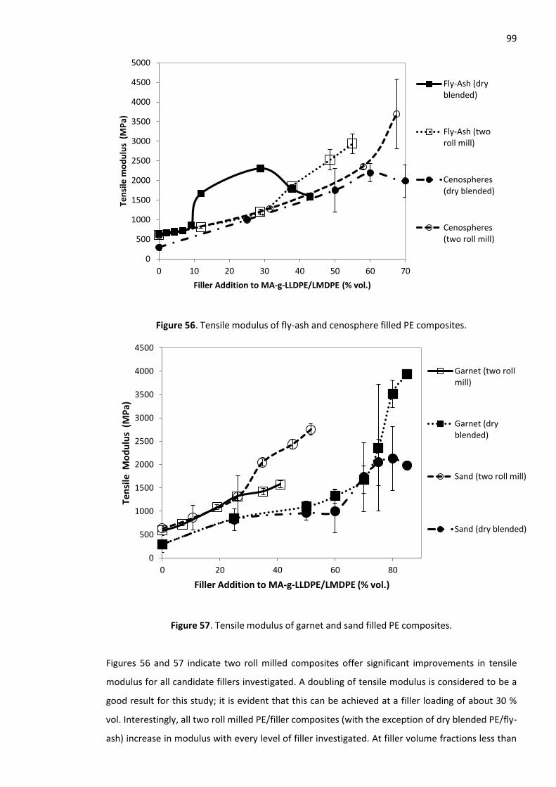
99

Figure 56. Tensile modulus of fly-ash and cenosphere filled PE composites.

Figure 57. Tensile modulus of garnet and sand filled PE composites.

Figures 56 and 57 indicate two roll milled composites offer significant improvements in tensile

modulus for all candidate fillers investigated. A doubling of tensile modulus is considered to be a

good result for this study; it is evident that this can be achieved at a filler loading of about 30 %

vol. Interestingly, all two roll milled PE/filler composites (with the exception of dry blended PE/fly-

ash) increase in modulus with every level of filler investigated. At filler volume fractions less than

0

500

1000

1500

2000

2500

3000

3500

4000

4500

5000

0 10 20 30 40 50 60 70

Ten

sile

mo

du

lus

(M

Pa)

Filler Addition to MA-g-LLDPE/LMDPE (% vol.)

Fly-Ash (dryblended)

Fly-Ash (tworoll mill)

Cenospheres(dry blended)

Cenospheres(two roll mill)

0

500

1000

1500

2000

2500

3000

3500

4000

4500

0 20 40 60 80

Ten

sile

Mo

du

lus

(M

Pa)

Filler Addition to MA-g-LLDPE/LMDPE (% vol.)

Garnet (two rollmill)

Garnet (dryblended)

Sand (two roll mill)

Sand (dry blended)

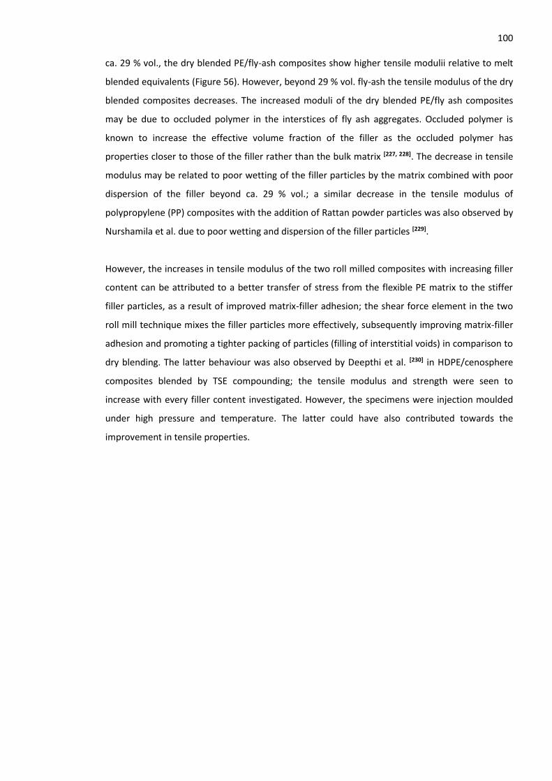
100 ca. 29 % vol., the dry blended PE/fly-ash composites show higher tensile modulii relative to melt

blended equivalents (Figure 56). However, beyond 29 % vol. fly-ash the tensile modulus of the dry

blended composites decreases. The increased moduli of the dry blended PE/fly ash composites

may be due to occluded polymer in the interstices of fly ash aggregates. Occluded polymer is

known to increase the effective volume fraction of the filler as the occluded polymer has

properties closer to those of the filler rather than the bulk matrix [227, 228]. The decrease in tensile

modulus may be related to poor wetting of the filler particles by the matrix combined with poor

dispersion of the filler beyond ca. 29 % vol.; a similar decrease in the tensile modulus of

polypropylene (PP) composites with the addition of Rattan powder particles was also observed by

Nurshamila et al. due to poor wetting and dispersion of the filler particles [229].

However, the increases in tensile modulus of the two roll milled composites with increasing filler

content can be attributed to a better transfer of stress from the flexible PE matrix to the stiffer

filler particles, as a result of improved matrix-filler adhesion; the shear force element in the two

roll mill technique mixes the filler particles more effectively, subsequently improving matrix-filler

adhesion and promoting a tighter packing of particles (filling of interstitial voids) in comparison to

dry blending. The latter behaviour was also observed by Deepthi et al. [230] in HDPE/cenosphere

composites blended by TSE compounding; the tensile modulus and strength were seen to

increase with every filler content investigated. However, the specimens were injection moulded

under high pressure and temperature. The latter could have also contributed towards the

improvement in tensile properties.

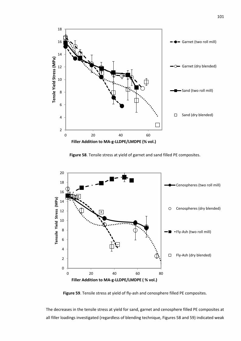
101

Figure 58. Tensile stress at yield of garnet and sand filled PE composites.

Figure 59. Tensile stress at yield of fly-ash and cenosphere filled PE composites.

The decreases in the tensile stress at yield for sand, garnet and cenosphere filled PE composites at

all filler loadings investigated (regardless of blending technique, Figures 58 and 59) indicated weak

2

4

6

8

10

12

14

16

18

0 20 40 60

Ten

sle

Yie

ld S

tres

s (M

Pa)

Filler Addition to MA-g-LLDPE/LMDPE (% vol.)

Garnet (two roll mill)

Garnet (dry blended)

Sand (two roll mill)

Sand (dry blended)

0

2

4

6

8

10

12

14

16

18

20

0 20 40 60 80

Ten

ssile

Yie

ld S

tre

ss (

MP

a)

Filler Addition to MA-g-LLDPE/LMDPE ( % vol.)

Cenospheres (two roll mill)

Cenospheres (dry blended)

Fly-Ash (two roll mill)

Fly-Ash (dry blended)

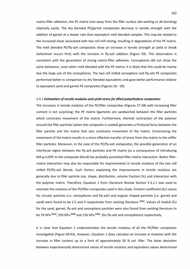
102 matrix-filler adhesion; the PE matrix tore away from the filler surface (de-wetting or de-bonding)

relatively easily. The dry blended PE/garnet composites decrease in tensile strength with the

addition of garnet at a slower rate than equivalent melt blended samples. This may be related to

the increased shear associated with two roll mill mixing, resulting in degradation of the PE matrix.

The melt blended PE/fly-ash composites show an increase in tensile strength at yield or break

(whichever occurs first) with the increase in fly-ash addition (Figure 59). This observation is

consistent with the generation of strong matrix-filler adhesion. Cenospheres did not show the

same behaviour, even when melt blended with the PE matrix. It is likely that this could be mainly

due the large size of the cenospheres. The two roll milled cenosphere and fly-ash PE composites

performed better in comparison to dry blended equivalents and gave better performance relative

to equivalent sand and garnet PE composites (Figures 56 - 59).

5.4.1 Estimation of tensile modulus and yield stress for filled polyethylene composites

The increases in tensile modulus of the PE/filler composites (Figures 57-58) with increasing filler

content is not surprising; the PE matrix ligaments are sandwiched between the filler particles

which constrains movement of the matrix. Furthermore, thermal contraction of the polymer

around the filler particles (when the composite is cooled) generates a frictional force between the

filler particle and the matrix that also constrains movement of the matrix. Constraining the

movement of the matrix results in a more effective transfer of stress from the matrix to the stiffer

filler particles. Moreover, in the case of the PE/fly-ash composites, the possible generation of an

interfacial region between the fly-ash particles and PE matrix (as a consequence of introducing

MA-g-LLDPE to the composite blend) has probably promoted filler-matrix interaction. Better filler-

matrix interaction may also be responsible for improvements in tensile modulus of the two roll

milled PE/fly-ash blends. Such factors explaining the improvements in tensile modulus are

generally due to filler particle size, shape, distribution, volume fraction (Vf) and interaction with

the polymer matrix. Therefore, Equation 1 from Literature Review Section 3.3.1.1 was used to

estimate the modulus of the PE/filler composites used in this study. Einstein coefficient (KE) values

for circular particles (i.e. cenospheres and fly-ash) and angular shaped particles (i.e. garnet and

sand) were found to be 2.5 and 4 respectively from existing literature [101]. Values of moduli (Ef)

for the sand, garnet, fly-ash and cenosphere particles were also found from existing literature to

be 70 GPa [231], 250 GPa [232] and 150 GPa [233] (for fly-ash and cenospheres) respectively.

It is clear that Equation 1 underestimates the tensile modulus of all the PE/filler composites

investigated (Figure 60-63). However, Equation 1 does calculate an increase in modulus with the

increase in filler content up to a limit of approximately 50 % vol. filler. The latter deviation

between experimentally determined values of tensile modulus and equivalent values determined

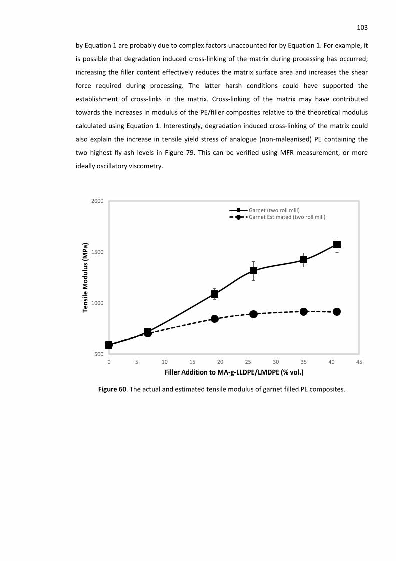
103 by Equation 1 are probably due to complex factors unaccounted for by Equation 1. For example, it

is possible that degradation induced cross-linking of the matrix during processing has occurred;

increasing the filler content effectively reduces the matrix surface area and increases the shear

force required during processing. The latter harsh conditions could have supported the

establishment of cross-links in the matrix. Cross-linking of the matrix may have contributed

towards the increases in modulus of the PE/filler composites relative to the theoretical modulus

calculated using Equation 1. Interestingly, degradation induced cross-linking of the matrix could

also explain the increase in tensile yield stress of analogue (non-maleanised) PE containing the

two highest fly-ash levels in Figure 79. This can be verified using MFR measurement, or more

ideally oscillatory viscometry.

Figure 60. The actual and estimated tensile modulus of garnet filled PE composites.

500

1000

1500

2000

0 5 10 15 20 25 30 35 40 45

Ten

sile

Mo

du

lus

(MP

a)

Filler Addition to MA-g-LLDPE/LMDPE (% vol.)

Garnet (two roll mill)Garnet Estimated (two roll mill)

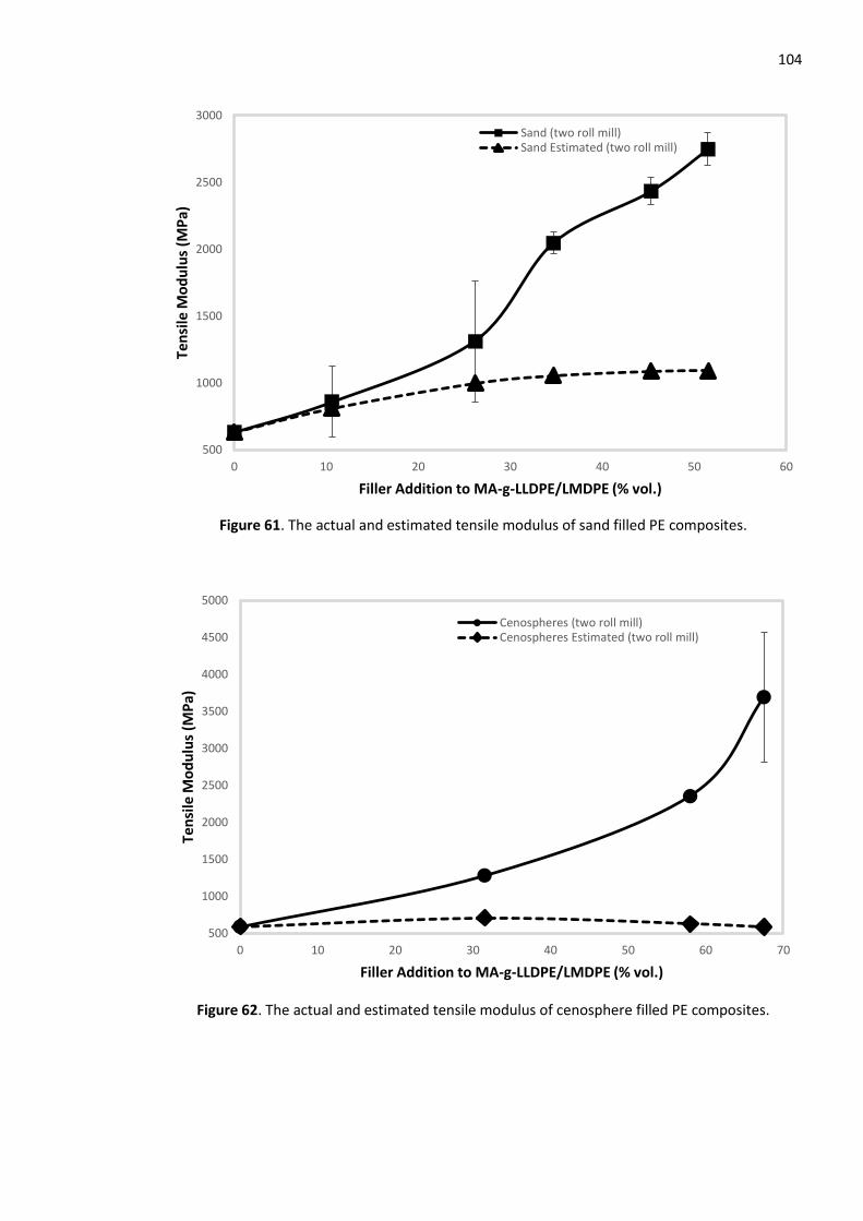
104

Figure 61. The actual and estimated tensile modulus of sand filled PE composites.

Figure 62. The actual and estimated tensile modulus of cenosphere filled PE composites.

500

1000

1500

2000

2500

3000

0 10 20 30 40 50 60

Ten

sile

Mo

du

lus

(MP

a)

Filler Addition to MA-g-LLDPE/LMDPE (% vol.)

Sand (two roll mill)Sand Estimated (two roll mill)

500

1000

1500

2000

2500

3000

3500

4000

4500

5000

0 10 20 30 40 50 60 70

Ten

sile

Mo

du

lus

(MP

a)

Filler Addition to MA-g-LLDPE/LMDPE (% vol.)

Cenospheres (two roll mill)Cenospheres Estimated (two roll mill)

105

Figure 63. The actual and estimated tensile modulus of fly-ash filled PE composites.

The decrease in tensile yield stress of the large particle garnet, sand and cenosphere PE

composites with increasing filler level is unsurprising; little interaction was observed between the

latter filler particles and MA-g-LLDPE/LMDPE (Figures 58 and 59). At low filler levels this was

especially true; the ductile PE matrix withstood the majority of the stress in the composite and

continued to deform post-yield. However, at higher filler loadings the matrix yielded

simultaneously with filler-matrix de-bonding and fractured, due to the loss in matrix surface area

within the composite. The loss in matrix surface area can be calculated by 1 minus the volume

fraction of filler (1 - Vf) [234]. Therefore, Equation 2 (Literature Review Section 3.3.1.2) was used to

estimate the yield stress of the two roll mill blended PE/filler composites detailed in Table 10.

Figures 64 - 67 show both the actual and estimated tensile yield stress of the PE/filler composites

with the increase in filler content. It is apparent that Equation 2 provided a reasonably accurate

approximation of yield stress for the garnet, sand and cenosphere PE composites at filler levels

below approximately 35 % vol. At filler levels above 35 % vol. Equation 2 underestimated the yield

stress of the composite; at higher filler levels the latter PE/filler composites fracture, this switch

over from ductile behaviour at yield (with the lower levels of filler) to brittle failure (with the high

levels of filler beyond ca. 35 % vol.) indicates that, even though little or no matrix-filler interaction

is present, the relatively high volume of filler is providing some modulus enhancement to the

composite. In the case of the PE/fly-ash composites (Figure 67), Equation 2 severely

underestimates the tensile yield stress; due to well-established interfacial regions between the

500

1000

1500

2000

2500

3000

3500

0 10 20 30 40 50 60

Ten

sile

Mo

du

lus

(MP

a)

Filler Addition to MA-g-LLDPE/LMDPE (% vol.)

Fly-ash (two roll mill)Fly-ash Estimated (two roll mill)

106 fly-ash particles and the MA-g-LLDPE/LMDPE matrix, the PE/fly-ash composites actually increase

in tensile yield stress, a factor which is unaccounted for in Equation 2. However, It appears that

Equation 2 provides good approximations of yield stress for relatively low to medium filled

polymer composites (below 40 % vol.) if little or no matrix-filler interaction is assumed. On the

other hand, in the case of highly filled composites or filled composites with better matrix-filler

interaction, the shape, size, dispersion, orientation, yield stress of the filler particles and strength

of matrix-filler interaction play a more influential role in estimating the yield stress of filled

polymer composites [235].

Figure 64. The actual and estimated tensile yield stress of garnet filled PE composites.

4

6

8

10

12

14

16

18

0 10 20 30 40 50

Ten

sle

Yie

ld S

tre

ss (

MP

a)

Filler Addition to MA-g-LLDPE/LMDPE (% vol.)

Garnet (two roll mill)

Garnet Estimated (two rollmill)

107

Figure 65. The actual and estimated tensile yield stress of sand filled PE composites

Figure 66. The actual and estimated tensile yield stress of cenosphere filled PE composites.

2

4

6

8

10

12

14

16

18

0 20 40 60

Ten

sle

Yie

ld S

tres

s (M

Pa)

Filler Addition to MA-g-LLDPE/LMDPE (% vol.)

Sand (two roll mill)

Sand Estimated (two rollmill)

0

2

4

6

8

10

12

14

16

18

0 20 40 60 80

Ten

ssile

Yie

ld S

tre

ss (

MP

a)

Filler Addition to MA-g-LLDPE/LMDPE ( % vol.)

Cenospheres (two rollmill)

Cenospheres Estimated(two roll mill)

108

Figure 67. The actual and estimated tensile yield stress of fly-ash filled PE composites

.

5.4.2 Key findings from the comparison of composite formation processes

Investigating the effect of various polymer-filler blending methods forms another particularly

novel aspect of this research in the context of rotational moulding. For the purpose of clarity, the

key findings of this investigation are summarised in the following bullet points:

The two roll milled composites offer significant improvements in tensile modulus for all

candidate fillers investigated. A doubling of tensile modulus is considered to be a good

result for this study; it is evident that this can be achieved at a filler loading of about 30 %

vol. Interestingly, all two roll milled PE/filler composites (with the exception of dry

blended PE/fly-ash) increase in modulus with every level of filler investigated.

At filler volume fractions less than ca. 29 % vol., the dry blended PE/fly-ash composites

have higher tensile modulii relative to melt blended equivalents. However, beyond 29 %

vol. fly-ash the tensile modulus of the dry blended composites decreases; the decrease in

tensile modulus observed may be related to poor wetting combined with poor dispersion

of the filler beyond ca. 29 % vol.

The increases in tensile modulus of the two roll milled composites with increasing filler

content can be attributed to a better transfer of stress from the flexible PE matrix to the

stiffer filler particles, as a result of improved matrix-filler adhesion. The shear force

element in the two roll mill technique could promote better mixing of filler particles,

2

4

6

8

10

12

14

16

18

20

22

0 10 20 30 40 50 60

Ten

ssile

Yie

ld S

tres

s (

MP

a)

Filler Addition to MA-g-LLDPE/LMDPE ( % vol.)

Fly-Ash (two roll mill)

Fly-ash Estimated (two rollmill)

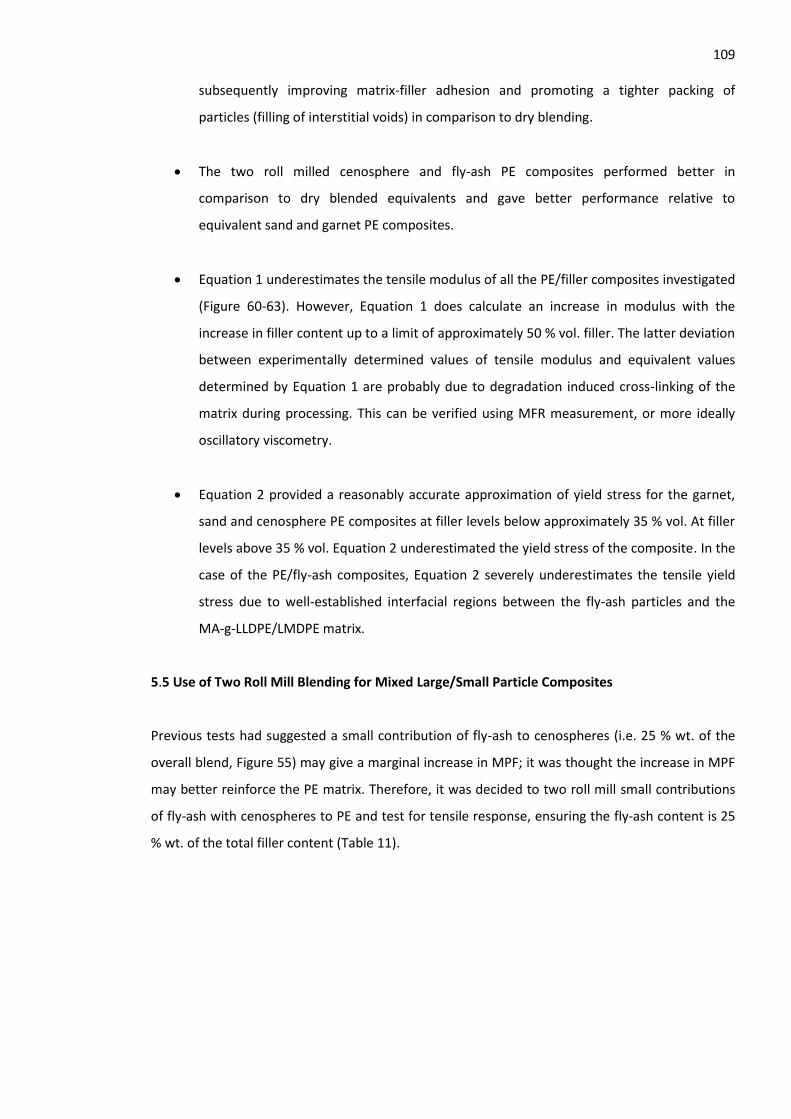
109

subsequently improving matrix-filler adhesion and promoting a tighter packing of

particles (filling of interstitial voids) in comparison to dry blending.

The two roll milled cenosphere and fly-ash PE composites performed better in

comparison to dry blended equivalents and gave better performance relative to

equivalent sand and garnet PE composites.

Equation 1 underestimates the tensile modulus of all the PE/filler composites investigated

(Figure 60-63). However, Equation 1 does calculate an increase in modulus with the

increase in filler content up to a limit of approximately 50 % vol. filler. The latter deviation

between experimentally determined values of tensile modulus and equivalent values

determined by Equation 1 are probably due to degradation induced cross-linking of the

matrix during processing. This can be verified using MFR measurement, or more ideally

oscillatory viscometry.

Equation 2 provided a reasonably accurate approximation of yield stress for the garnet,

sand and cenosphere PE composites at filler levels below approximately 35 % vol. At filler

levels above 35 % vol. Equation 2 underestimated the yield stress of the composite. In the

case of the PE/fly-ash composites, Equation 2 severely underestimates the tensile yield

stress due to well-established interfacial regions between the fly-ash particles and the

MA-g-LLDPE/LMDPE matrix.

5.5 Use of Two Roll Mill Blending for Mixed Large/Small Particle Composites

Previous tests had suggested a small contribution of fly-ash to cenospheres (i.e. 25 % wt. of the

overall blend, Figure 55) may give a marginal increase in MPF; it was thought the increase in MPF

may better reinforce the PE matrix. Therefore, it was decided to two roll mill small contributions

of fly-ash with cenospheres to PE and test for tensile response, ensuring the fly-ash content is 25

% wt. of the total filler content (Table 11).

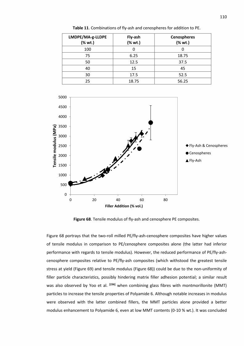
110

Table 11. Combinations of fly-ash and cenospheres for addition to PE.

LMDPE/MA-g-LLDPE (% wt.)

Fly-ash (% wt.)

Cenospheres (% wt.)

100 0 0

75 6.25 18.75

50 12.5 37.5

40 15 45

30 17.5 52.5

25 18.75 56.25

Figure 68. Tensile modulus of fly-ash and cenosphere PE composites.

Figure 68 portrays that the two-roll milled PE/fly-ash-cenosphere composites have higher values

of tensile modulus in comparison to PE/cenosphere composites alone (the latter had inferior

performance with regards to tensile modulus). However, the reduced performance of PE/fly-ash-

cenosphere composites relative to PE/fly-ash composites (which withstood the greatest tensile

stress at yield (Figure 69) and tensile modulus (Figure 68)) could be due to the non-uniformity of

filler particle characteristics, possibly hindering matrix filler adhesion potential; a similar result

was also observed by Yoo et al. [236] when combining glass fibres with montmorillonite (MMT)

particles to increase the tensile properties of Polyamide 6. Although notable increases in modulus

were observed with the latter combined fillers, the MMT particles alone provided a better

modulus enhancement to Polyamide 6, even at low MMT contents (0-10 % wt.). It was concluded

0

500

1000

1500

2000

2500

3000

3500

4000

4500

5000

0 20 40 60 80

Ten

sile

mo

du

lus

(MP

a)

Filler Addition (% vol.)

Fly-Ash & Cenospheres

Cenospheres

Fly-Ash

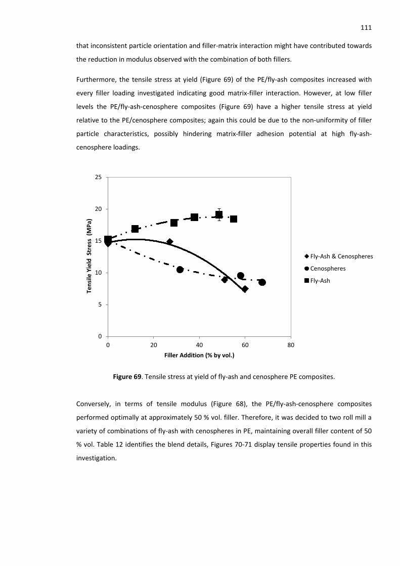
111 that inconsistent particle orientation and filler-matrix interaction might have contributed towards

the reduction in modulus observed with the combination of both fillers.

Furthermore, the tensile stress at yield (Figure 69) of the PE/fly-ash composites increased with

every filler loading investigated indicating good matrix-filler interaction. However, at low filler

levels the PE/fly-ash-cenosphere composites (Figure 69) have a higher tensile stress at yield

relative to the PE/cenosphere composites; again this could be due to the non-uniformity of filler

particle characteristics, possibly hindering matrix-filler adhesion potential at high fly-ash-

cenosphere loadings.

Figure 69. Tensile stress at yield of fly-ash and cenosphere PE composites.

Conversely, in terms of tensile modulus (Figure 68), the PE/fly-ash-cenosphere composites

performed optimally at approximately 50 % vol. filler. Therefore, it was decided to two roll mill a

variety of combinations of fly-ash with cenospheres in PE, maintaining overall filler content of 50

% vol. Table 12 identifies the blend details, Figures 70-71 display tensile properties found in this

investigation.

0

5

10

15

20

25

0 20 40 60 80

Ten

sile

Yie

ld S

tre

ss (

MP

a)

Filler Addition (% by vol.)

Fly-Ash & Cenospheres

Cenospheres

Fly-Ash

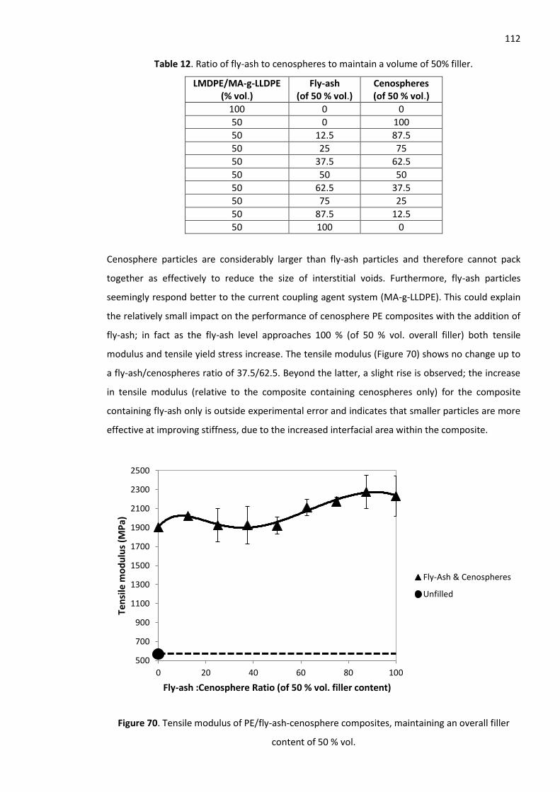
112

Table 12. Ratio of fly-ash to cenospheres to maintain a volume of 50% filler.

LMDPE/MA-g-LLDPE (% vol.)

Fly-ash (of 50 % vol.)

Cenospheres (of 50 % vol.)

100 0 0

50 0 100

50 12.5 87.5

50 25 75

50 37.5 62.5

50 50 50

50 62.5 37.5

50 75 25

50 87.5 12.5

50 100 0

Cenosphere particles are considerably larger than fly-ash particles and therefore cannot pack

together as effectively to reduce the size of interstitial voids. Furthermore, fly-ash particles

seemingly respond better to the current coupling agent system (MA-g-LLDPE). This could explain

the relatively small impact on the performance of cenosphere PE composites with the addition of

fly-ash; in fact as the fly-ash level approaches 100 % (of 50 % vol. overall filler) both tensile

modulus and tensile yield stress increase. The tensile modulus (Figure 70) shows no change up to

a fly-ash/cenospheres ratio of 37.5/62.5. Beyond the latter, a slight rise is observed; the increase

in tensile modulus (relative to the composite containing cenospheres only) for the composite

containing fly-ash only is outside experimental error and indicates that smaller particles are more

effective at improving stiffness, due to the increased interfacial area within the composite.

Figure 70. Tensile modulus of PE/fly-ash-cenosphere composites, maintaining an overall filler

content of 50 % vol.

500

700

900

1100

1300

1500

1700

1900

2100

2300

2500

0 20 40 60 80 100

Ten

sile

mo

du

lus

(MP

a)

Fly-ash :Cenosphere Ratio (of 50 % vol. filler content)

Fly-Ash & Cenospheres

Unfilled

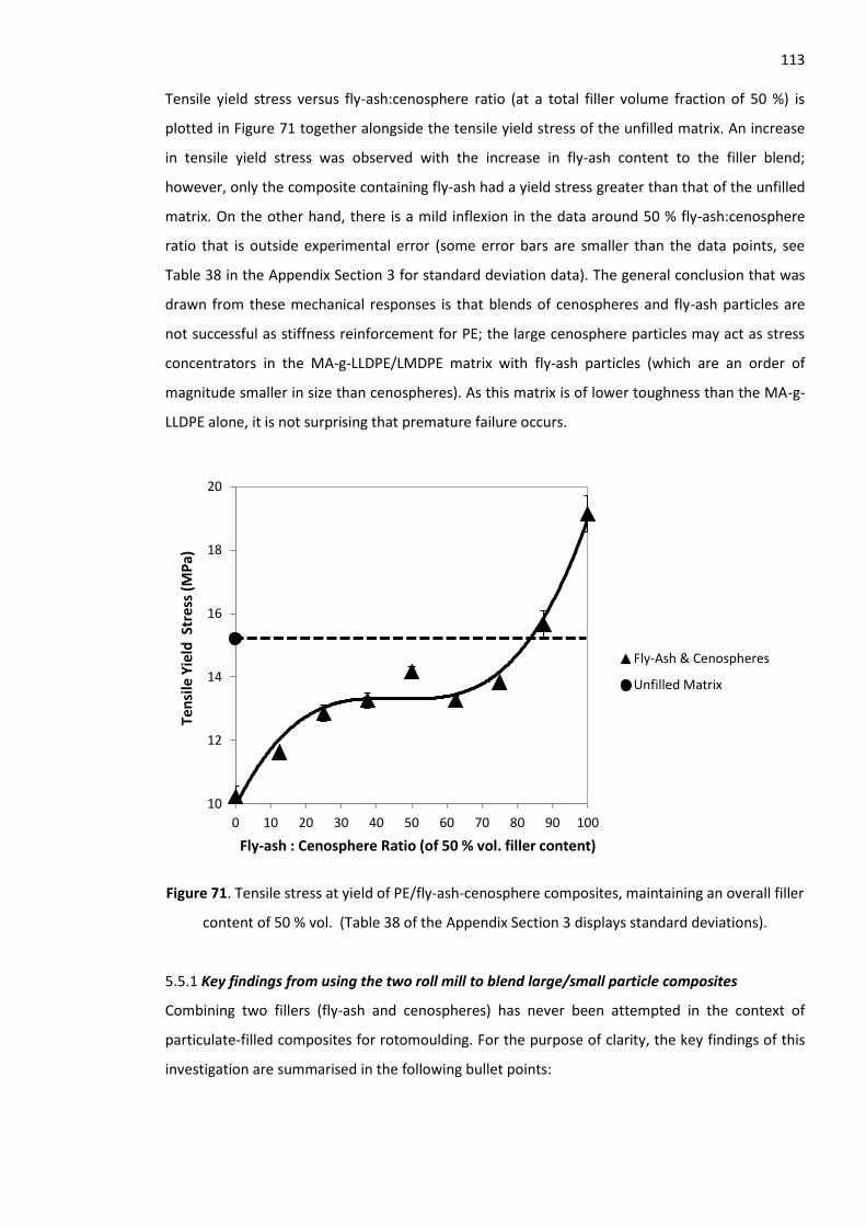
113 Tensile yield stress versus fly-ash:cenosphere ratio (at a total filler volume fraction of 50 %) is

plotted in Figure 71 together alongside the tensile yield stress of the unfilled matrix. An increase

in tensile yield stress was observed with the increase in fly-ash content to the filler blend;

however, only the composite containing fly-ash had a yield stress greater than that of the unfilled

matrix. On the other hand, there is a mild inflexion in the data around 50 % fly-ash:cenosphere

ratio that is outside experimental error (some error bars are smaller than the data points, see

Table 38 in the Appendix Section 3 for standard deviation data). The general conclusion that was

drawn from these mechanical responses is that blends of cenospheres and fly-ash particles are

not successful as stiffness reinforcement for PE; the large cenosphere particles may act as stress

concentrators in the MA-g-LLDPE/LMDPE matrix with fly-ash particles (which are an order of

magnitude smaller in size than cenospheres). As this matrix is of lower toughness than the MA-g-

LLDPE alone, it is not surprising that premature failure occurs.

Figure 71. Tensile stress at yield of PE/fly-ash-cenosphere composites, maintaining an overall filler

content of 50 % vol. (Table 38 of the Appendix Section 3 displays standard deviations).

5.5.1 Key findings from using the two roll mill to blend large/small particle composites

Combining two fillers (fly-ash and cenospheres) has never been attempted in the context of

particulate-filled composites for rotomoulding. For the purpose of clarity, the key findings of this

investigation are summarised in the following bullet points:

10

12

14

16

18

20

0 10 20 30 40 50 60 70 80 90 100

Ten

sile

Yie

ld S

tre

ss (

MP

a)

Fly-ash : Cenosphere Ratio (of 50 % vol. filler content)

Fly-Ash & Cenospheres

Unfilled Matrix

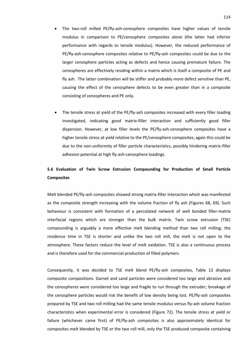
114

The two-roll milled PE/fly-ash-cenosphere composites have higher values of tensile

modulus in comparison to PE/cenosphere composites alone (the latter had inferior

performance with regards to tensile modulus). However, the reduced performance of

PE/fly-ash-cenosphere composites relative to PE/fly-ash composites could be due to the

larger cenosphere particles acting as defects and hence causing premature failure. The

cenospheres are effectively residing within a matrix which is itself a composite of PE and

fly ash. The latter combination will be stiffer and probably more defect sensitive than PE,

causing the effect of the cenosphere defects to be even greater than in a composite

consisting of cenospheres and PE only.

The tensile stress at yield of the PE/fly-ash composites increased with every filler loading

investigated, indicating good matrix-filler interaction and sufficiently good filler

dispersion. However, at low filler levels the PE/fly-ash-cenosphere composites have a

higher tensile stress at yield relative to the PE/cenosphere composites; again this could be

due to the non-uniformity of filler particle characteristics, possibly hindering matrix-filler

adhesion potential at high fly-ash-cenosphere loadings.

5.6 Evaluation of Twin Screw Extrusion Compounding for Production of Small Particle

Composites

Melt blended PE/fly-ash composites showed strong matrix-filler interaction which was manifested

as the composite strength increasing with the volume fraction of fly ash (Figures 68, 69). Such

behaviour is consistent with formation of a percolated network of well bonded filler-matrix

interfacial regions which are stronger than the bulk matrix. Twin screw extrusion (TSE)

compounding is arguably a more effective melt blending method than two roll milling; the

residence time in TSE is shorter and unlike the two roll mill, the melt is not open to the

atmosphere. These factors reduce the level of melt oxidation. TSE is also a continuous process

and is therefore used for the commercial production of filled polymers.

Consequently, it was decided to TSE melt blend PE/fly-ash composites, Table 13 displays

composite compositions. Garnet and sand particles were considered too large and abrasive and

the cenospheres were considered too large and fragile to run through the extruder; breakage of

the cenosphere particles would risk the benefit of low density being lost. PE/fly-ash composites

prepared by TSE and two roll milling had the same tensile modulus versus fly-ash volume fraction

characteristics when experimental error is considered (Figure 72). The tensile stress at yield or

failure (whichever came first) of PE/fly-ash composites is also approximately identical for

composites melt blended by TSE or the two roll mill, only the TSE produced composite containing

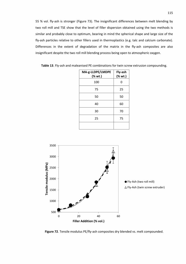
115 55 % vol. fly-ash is stronger (Figure 73). The insignificant differences between melt blending by

two roll mill and TSE show that the level of filler dispersion obtained using the two methods is

similar and probably close to optimum, bearing in mind the spherical shape and large size of the

fly-ash particles relative to other fillers used in thermoplastics (e.g. talc and calcium carbonate).

Differences in the extent of degradation of the matrix in the fly-ash composites are also

insignificant despite the two roll mill blending process being open to atmospheric oxygen.

Table 13. Fly-ash and maleanised PE combinations for twin screw extrusion compounding.

MA-g-LLDPE/LMDPE (% wt.)

Fly-ash (% wt.)

100 0

75 25

50 50

40 60

30 70

25 75

Figure 72. Tensile modulus PE/fly-ash composites dry blended vs. melt compounded.

500

1000

1500

2000

2500

3000

3500

0 20 40 60

Ten

sile

mo

du

lus

(MP

a)

Filler Addition (% vol.)

Fly-Ash (two roll mill)

Fly-Ash (twin screw extruder)

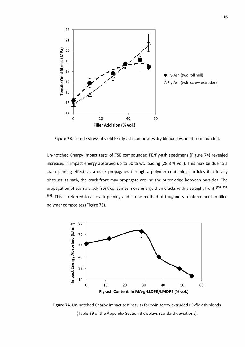
116

Figure 73. Tensile stress at yield PE/fly-ash composites dry blended vs. melt compounded.

Un-notched Charpy impact tests of TSE compounded PE/fly-ash specimens (Figure 74) revealed

increases in impact energy absorbed up to 50 % wt. loading (28.8 % vol.). This may be due to a

crack pinning effect; as a crack propagates through a polymer containing particles that locally

obstruct its path, the crack front may propagate around the outer edge between particles. The

propagation of such a crack front consumes more energy than cracks with a straight front [237, 238,

239]. This is referred to as crack pinning and is one method of toughness reinforcement in filled

polymer composites (Figure 75).

Figure 74. Un-notched Charpy impact test results for twin screw extruded PE/fly-ash blends.

(Table 39 of the Appendix Section 3 displays standard deviations).

14

15

16

17

18

19

20

21

22

0 20 40 60

Ten

sile

Yie

ld S

tre

ss (

MP

a)

Filler Addition (% vol.)

Fly-Ash (two roll mill)

Fly-Ash (twin screw extruder)

10

25

40

55

70

85

0 10 20 30 40 50 60

Imp

act

Ener

gy A

bso

rbed

(kJ

m-2

)

Fly-ash Content in MA-g-LLDPE/LMDPE (% vol.)

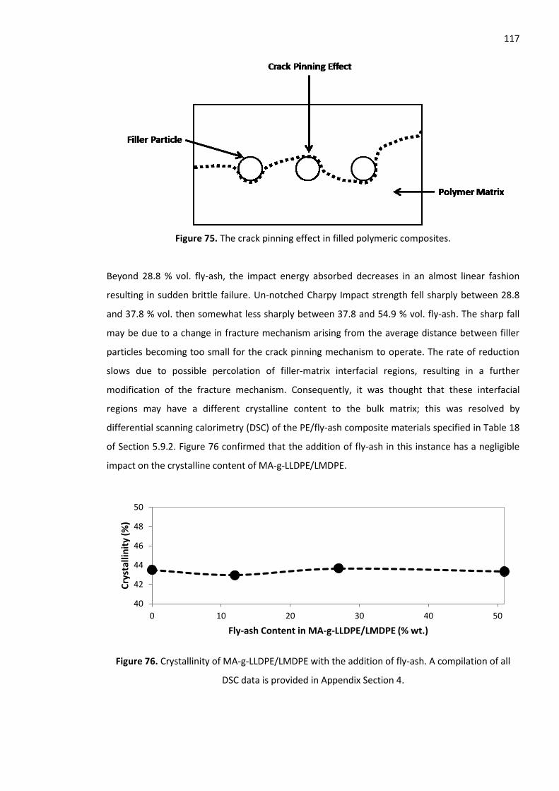
117

Figure 75. The crack pinning effect in filled polymeric composites.

Beyond 28.8 % vol. fly-ash, the impact energy absorbed decreases in an almost linear fashion

resulting in sudden brittle failure. Un-notched Charpy Impact strength fell sharply between 28.8

and 37.8 % vol. then somewhat less sharply between 37.8 and 54.9 % vol. fly-ash. The sharp fall

may be due to a change in fracture mechanism arising from the average distance between filler

particles becoming too small for the crack pinning mechanism to operate. The rate of reduction

slows due to possible percolation of filler-matrix interfacial regions, resulting in a further

modification of the fracture mechanism. Consequently, it was thought that these interfacial

regions may have a different crystalline content to the bulk matrix; this was resolved by

differential scanning calorimetry (DSC) of the PE/fly-ash composite materials specified in Table 18

of Section 5.9.2. Figure 76 confirmed that the addition of fly-ash in this instance has a negligible

impact on the crystalline content of MA-g-LLDPE/LMDPE.

Figure 76. Crystallinity of MA-g-LLDPE/LMDPE with the addition of fly-ash. A compilation of all

DSC data is provided in Appendix Section 4.

40

42

44

46

48

50

0 10 20 30 40 50

Cry

stal

linit

y (%

)

Fly-ash Content in MA-g-LLDPE/LMDPE (% wt.)

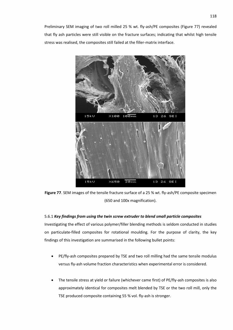
118 Preliminary SEM imaging of two roll milled 25 % wt. fly-ash/PE composites (Figure 77) revealed

that fly ash particles were still visible on the fracture surfaces; indicating that whilst high tensile

stress was realised, the composites still failed at the filler-matrix interface.

Figure 77. SEM images of the tensile fracture surface of a 25 % wt. fly-ash/PE composite specimen

(650 and 100x magnification).

5.6.1 Key findings from using the twin screw extruder to blend small particle composites

Investigating the effect of various polymer/filler blending methods is seldom conducted in studies

on particulate-filled composites for rotational moulding. For the purpose of clarity, the key

findings of this investigation are summarised in the following bullet points:

PE/fly-ash composites prepared by TSE and two roll milling had the same tensile modulus

versus fly-ash volume fraction characteristics when experimental error is considered.

The tensile stress at yield or failure (whichever came first) of PE/fly-ash composites is also

approximately identical for composites melt blended by TSE or the two roll mill, only the

TSE produced composite containing 55 % vol. fly-ash is stronger.

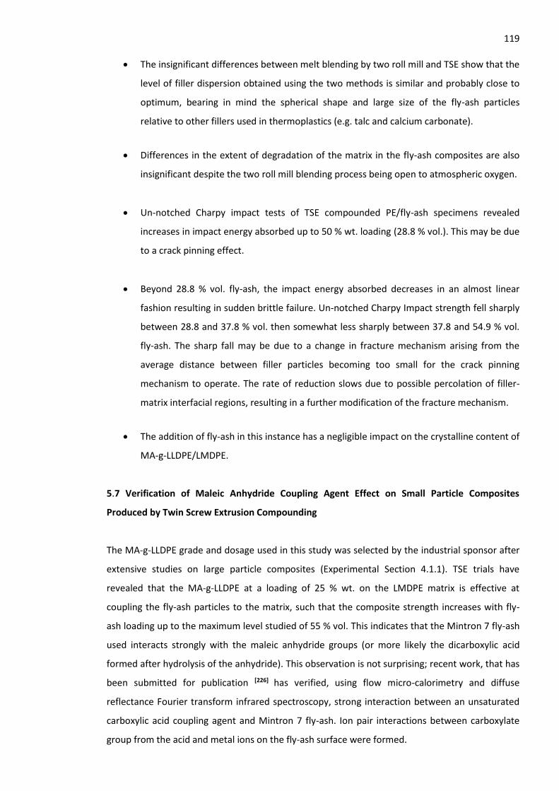
119

The insignificant differences between melt blending by two roll mill and TSE show that the

level of filler dispersion obtained using the two methods is similar and probably close to

optimum, bearing in mind the spherical shape and large size of the fly-ash particles

relative to other fillers used in thermoplastics (e.g. talc and calcium carbonate).

Differences in the extent of degradation of the matrix in the fly-ash composites are also

insignificant despite the two roll mill blending process being open to atmospheric oxygen.

Un-notched Charpy impact tests of TSE compounded PE/fly-ash specimens revealed

increases in impact energy absorbed up to 50 % wt. loading (28.8 % vol.). This may be due

to a crack pinning effect.

Beyond 28.8 % vol. fly-ash, the impact energy absorbed decreases in an almost linear

fashion resulting in sudden brittle failure. Un-notched Charpy Impact strength fell sharply

between 28.8 and 37.8 % vol. then somewhat less sharply between 37.8 and 54.9 % vol.

fly-ash. The sharp fall may be due to a change in fracture mechanism arising from the

average distance between filler particles becoming too small for the crack pinning

mechanism to operate. The rate of reduction slows due to possible percolation of filler-

matrix interfacial regions, resulting in a further modification of the fracture mechanism.

The addition of fly-ash in this instance has a negligible impact on the crystalline content of

MA-g-LLDPE/LMDPE.

5.7 Verification of Maleic Anhydride Coupling Agent Effect on Small Particle Composites

Produced by Twin Screw Extrusion Compounding

The MA-g-LLDPE grade and dosage used in this study was selected by the industrial sponsor after

extensive studies on large particle composites (Experimental Section 4.1.1). TSE trials have

revealed that the MA-g-LLDPE at a loading of 25 % wt. on the LMDPE matrix is effective at

coupling the fly-ash particles to the matrix, such that the composite strength increases with fly-

ash loading up to the maximum level studied of 55 % vol. This indicates that the Mintron 7 fly-ash

used interacts strongly with the maleic anhydride groups (or more likely the dicarboxylic acid

formed after hydrolysis of the anhydride). This observation is not surprising; recent work, that has

been submitted for publication [226] has verified, using flow micro-calorimetry and diffuse

reflectance Fourier transform infrared spectroscopy, strong interaction between an unsaturated

carboxylic acid coupling agent and Mintron 7 fly-ash. Ion pair interactions between carboxylate

group from the acid and metal ions on the fly-ash surface were formed.

120 To further gauge the effectiveness of the maleanised PE on the properties of LMDPE/fly-ash

composites, it was decided to blend the PE/fly-ash composites in Table 13 using LMDPE

containing 25 % wt. of a similar non-maleanised LLDPE to the feedstock used to synthesise the

MA-g-LLDPE. The latter is termed “analogue PE”. It is well known the type of coupling agent and

amount used has an impact on the mechanical performance of particulate-filled polymer

composites. The current PE system is 25 % wt. MA-g-LLDPE with 75 % wt. LMDPE. It is reasonable

to assume a level of roughly 1 % by wt. maleic anhydride (MA) in the MA-g-LLDPE. However, the

exact level remains proprietary. Table 14 identifies blend information for this trial and Figures 78-

80 identify the tensile and impact properties.

Table 14. Fly-ash analogue PE combinations investigated.

Analogue PE (% wt.)

Fly-ash. (% wt.)

100 0

75 25

50 50

40 60

30 70

25 75

The tensile modulus of maleanised PE/fly-ash composites (Figure 78) is identical to that of

equivalent non-maleanised PE composites up to approximately 48 % vol. At the highest loadings

the analogue PE/fly-ash composites are slightly stiffer. This is probably due to a slightly higher

crystalline content in the interfacial region of the composites based on the analogue PE.

Attachment of the MA-g-LLDPE to the fly-ash particles may decrease crystallinity, reducing the

stiffness of the interfacial regions and tensile modulus; Hassan et al. [240] also observed a reduction

in the crystallinity of maleic anhydride grafted polypropylene (MA-g-PP)/glass fibre composites via

DSC examination, relative to equivalent composites without the MA coupling agent.

The tensile stress at yield or break (whichever comes first) is plotted against fly-ash volume

fraction in Figure 79; the MA-g-LLDPE modified composites increase in strength linearly (over the

range investigated) with increasing fly-ash level. In contrast, the composites modified with the

non-maleanised LLDPE show a decrease in strength which appears to be linear up to 38 % vol. fly-

ash. Interestingly, the analogue PE based composites containing the two highest fly-ash levels

show noticeably increased strength. This effect may be due to degradation induced cross-linking

of the matrix, it can be verified using MFR measurement, or more ideally oscillatory viscometry.

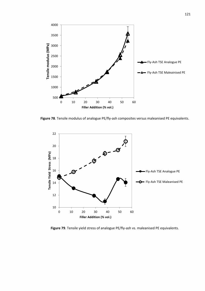
121

Figure 78. Tensile modulus of analogue PE/fly-ash composites versus maleanised PE equivalents.

Figure 79. Tensile yield stress of analogue PE/fly-ash vs. maleanised PE equivalents.

500

1000

1500

2000

2500

3000

3500

4000

0 10 20 30 40 50 60

Ten

sile

mo

du

lus

(MP

a)

Filler Addition (% vol.)

Fly-Ash TSE Analogue PE

Fly-Ash TSE Maleainised PE

10

12

14

16

18

20

22

0 10 20 30 40 50 60

Ten

sile

Yie

ld S

tre

ss (

MP

a)

Filler Addition (% vol.)

Fly-Ash TSE Analogue PE

Fly-Ash TSE Maleanised PE

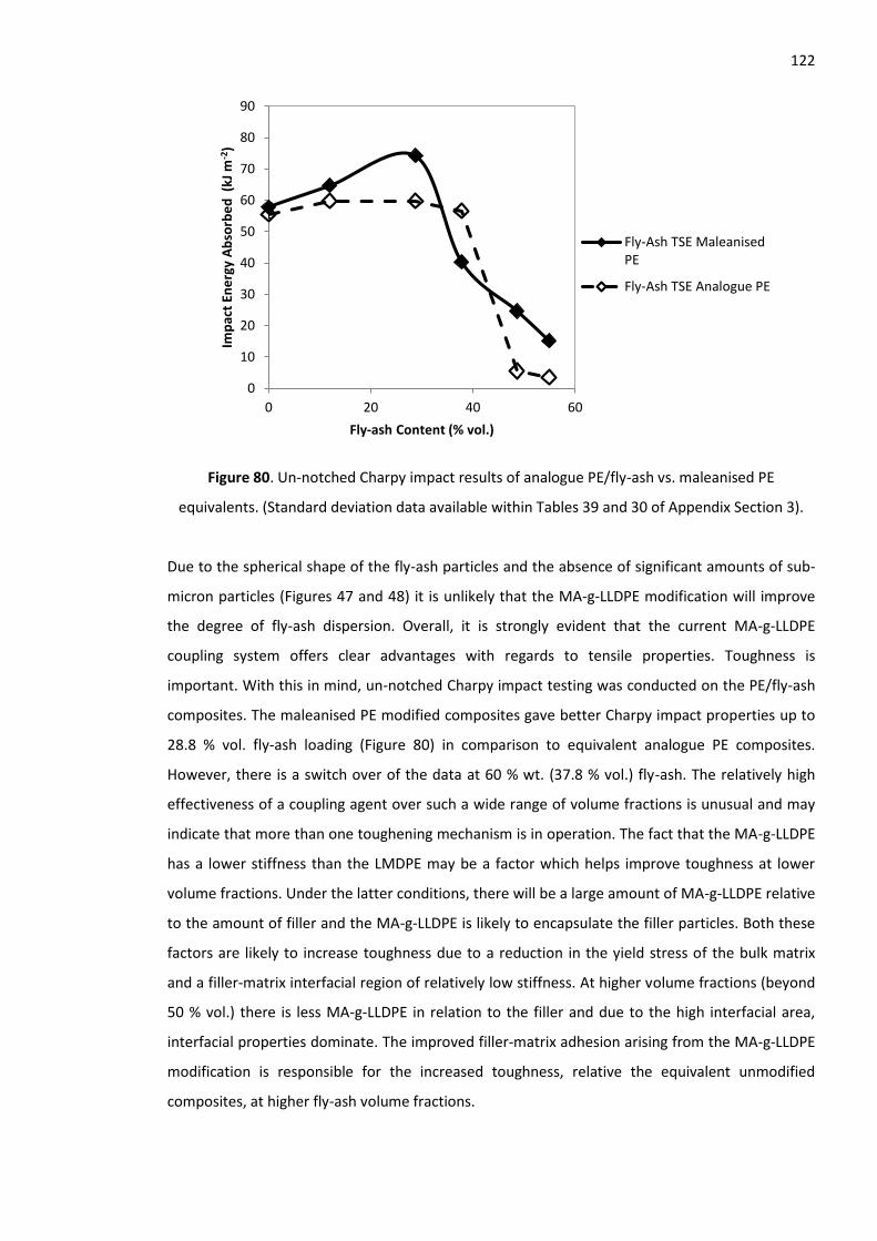
122

Figure 80. Un-notched Charpy impact results of analogue PE/fly-ash vs. maleanised PE

equivalents. (Standard deviation data available within Tables 39 and 30 of Appendix Section 3).

Due to the spherical shape of the fly-ash particles and the absence of significant amounts of sub-

micron particles (Figures 47 and 48) it is unlikely that the MA-g-LLDPE modification will improve

the degree of fly-ash dispersion. Overall, it is strongly evident that the current MA-g-LLDPE

coupling system offers clear advantages with regards to tensile properties. Toughness is

important. With this in mind, un-notched Charpy impact testing was conducted on the PE/fly-ash

composites. The maleanised PE modified composites gave better Charpy impact properties up to

28.8 % vol. fly-ash loading (Figure 80) in comparison to equivalent analogue PE composites.

However, there is a switch over of the data at 60 % wt. (37.8 % vol.) fly-ash. The relatively high

effectiveness of a coupling agent over such a wide range of volume fractions is unusual and may

indicate that more than one toughening mechanism is in operation. The fact that the MA-g-LLDPE

has a lower stiffness than the LMDPE may be a factor which helps improve toughness at lower

volume fractions. Under the latter conditions, there will be a large amount of MA-g-LLDPE relative

to the amount of filler and the MA-g-LLDPE is likely to encapsulate the filler particles. Both these

factors are likely to increase toughness due to a reduction in the yield stress of the bulk matrix

and a filler-matrix interfacial region of relatively low stiffness. At higher volume fractions (beyond

50 % vol.) there is less MA-g-LLDPE in relation to the filler and due to the high interfacial area,

interfacial properties dominate. The improved filler-matrix adhesion arising from the MA-g-LLDPE

modification is responsible for the increased toughness, relative the equivalent unmodified

composites, at higher fly-ash volume fractions.

0

10

20

30

40

50

60

70

80

90

0 20 40 60

Imp

act

Ene

rgy

Ab

sorb

ed

(kJ

m-2

)

Fly-ash Content (% vol.)

Fly-Ash TSE MaleanisedPE

Fly-Ash TSE Analogue PE

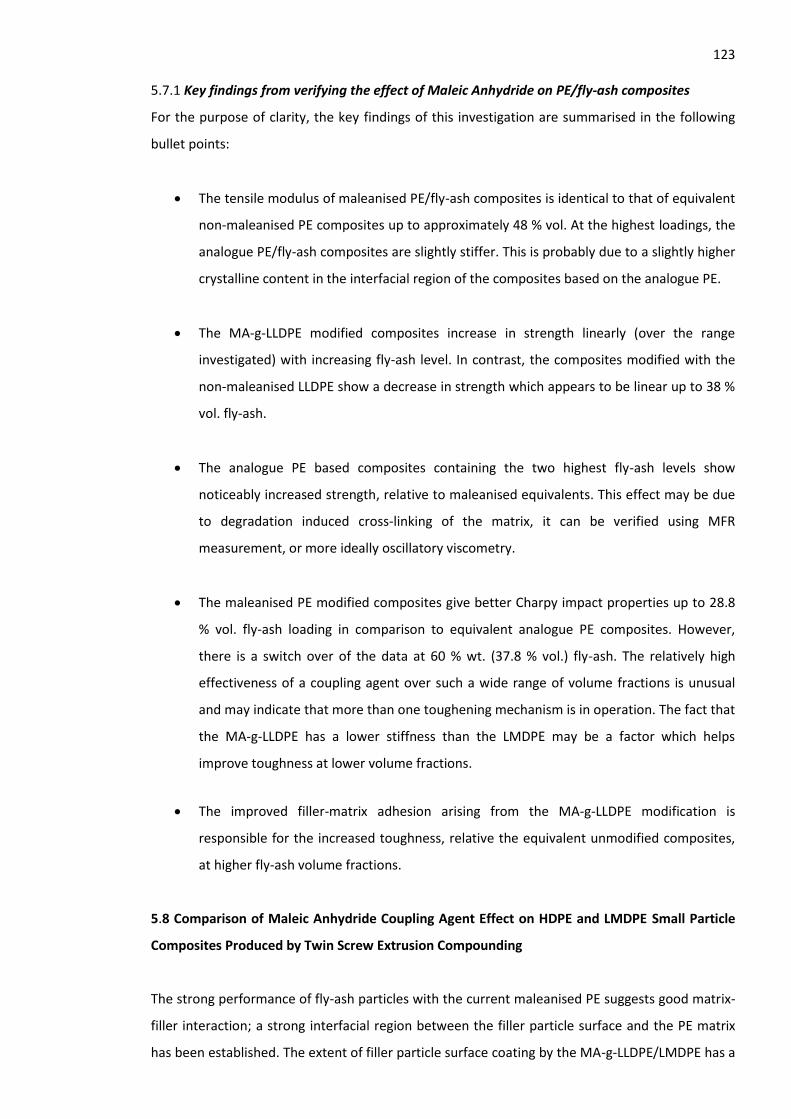
123 5.7.1 Key findings from verifying the effect of Maleic Anhydride on PE/fly-ash composites

For the purpose of clarity, the key findings of this investigation are summarised in the following

bullet points:

The tensile modulus of maleanised PE/fly-ash composites is identical to that of equivalent

non-maleanised PE composites up to approximately 48 % vol. At the highest loadings, the

analogue PE/fly-ash composites are slightly stiffer. This is probably due to a slightly higher

crystalline content in the interfacial region of the composites based on the analogue PE.

The MA-g-LLDPE modified composites increase in strength linearly (over the range

investigated) with increasing fly-ash level. In contrast, the composites modified with the

non-maleanised LLDPE show a decrease in strength which appears to be linear up to 38 %

vol. fly-ash.

The analogue PE based composites containing the two highest fly-ash levels show

noticeably increased strength, relative to maleanised equivalents. This effect may be due

to degradation induced cross-linking of the matrix, it can be verified using MFR

measurement, or more ideally oscillatory viscometry.

The maleanised PE modified composites give better Charpy impact properties up to 28.8

% vol. fly-ash loading in comparison to equivalent analogue PE composites. However,

there is a switch over of the data at 60 % wt. (37.8 % vol.) fly-ash. The relatively high

effectiveness of a coupling agent over such a wide range of volume fractions is unusual

and may indicate that more than one toughening mechanism is in operation. The fact that

the MA-g-LLDPE has a lower stiffness than the LMDPE may be a factor which helps

improve toughness at lower volume fractions.

The improved filler-matrix adhesion arising from the MA-g-LLDPE modification is

responsible for the increased toughness, relative the equivalent unmodified composites,

at higher fly-ash volume fractions.

5.8 Comparison of Maleic Anhydride Coupling Agent Effect on HDPE and LMDPE Small Particle

Composites Produced by Twin Screw Extrusion Compounding

The strong performance of fly-ash particles with the current maleanised PE suggests good matrix-

filler interaction; a strong interfacial region between the filler particle surface and the PE matrix

has been established. The extent of filler particle surface coating by the MA-g-LLDPE/LMDPE has a

124 profound effect on the physical properties of filled polymeric composites. In the case of PE/fly-ash

composites, increases in tensile modulus and stress at yield were seen with the increase in fly-ash

loading. Increases in Charpy impact properties were also observed up to 28.8 % vol. fly-ash. The

level of MA coupling agent in the MA-g-LLDPE used was originally found by experiment to be

optimum for large particle composites by the industrial sponsor Rotomotive Ltd. However, the fly-

ash particles are considerably smaller than the larger particle composites developed at

Rotomotive Ltd.

Therefore, the effect of MA-g-LLDPE on the tensile and impact properties of TSE melt blended,

compression moulded, 70 % wt. fly-ash filled LMDPE and HDPE was investigated (see Table 15);

the high 70 % wt. fly-ash loading was selected due to the exceptional improvements in stiffness

seen at that level for compression moulded materials. As rotational moulding is a zero shear

process, rudimentary rotational moulding and oven sintering trials were carried out by the

industrial partner; these trials revealed that whilst good mechanical properties were obtainable at

high filler levels with compression moulded plaques, a resistance to flow at zero shear placed a

question mark over the viability of using high filler loadings. Therefore, MFR tests were also

conducted on the resulting composites. However, it was appreciated that the MFR tests

conducted for this investigation were not under zero-shear conditions.

Table 15. Blend details of HDPE or LMDPE with Fly-ash

MA-g-LLDPE LMDPE or HDPE

with and without 70 % wt. fly-ash

(% wt.) (% wt.)

0 100

1 99

2.5 97.5

5 95

10 90

17.5 82.5

25 75

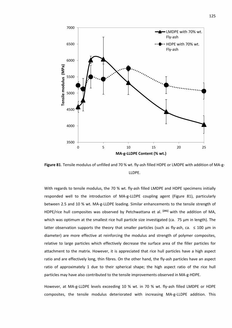
125

Figure 81. Tensile modulus of unfilled and 70 % wt. fly-ash filled HDPE or LMDPE with addition of MA-g-

LLDPE.

With regards to tensile modulus, the 70 % wt. fly-ash filled LMDPE and HDPE specimens initially

responded well to the introduction of MA-g-LLDPE coupling agent (Figure 81), particularly

between 2.5 and 10 % wt. MA-g-LLDPE loading. Similar enhancements to the tensile strength of

HDPE/rice hull composites was observed by Petchwattana et al. [241] with the addition of MA,

which was optimum at the smallest rice hull particle size investigated (ca. 75 µm in length). The

latter observation supports the theory that smaller particles (such as fly-ash, ca. ≤ 100 µm in

diameter) are more effective at reinforcing the modulus and strength of polymer composites,

relative to large particles which effectively decrease the surface area of the filler particles for

attachment to the matrix. However, it is appreciated that rice hull particles have a high aspect

ratio and are effectively long, thin fibres. On the other hand, the fly-ash particles have an aspect

ratio of approximately 1 due to their spherical shape; the high aspect ratio of the rice hull

particles may have also contributed to the tensile improvements observed in MA-g-HDPE.

However, at MA-g-LLDPE levels exceeding 10 % wt. in 70 % wt. fly-ash filled LMDPE or HDPE

composites, the tensile modulus deteriorated with increasing MA-g-LLDPE addition. This

3500

4000

4500

5000

5500

6000

6500

7000

0 5 10 15 20 25

Ten

sile

mo

du

lus

(M

Pa)

MA-g-LLDPE Content (% wt.)

LMDPE with 70% wt.Fly-ash

HDPE with 70% wt.Fly-ash

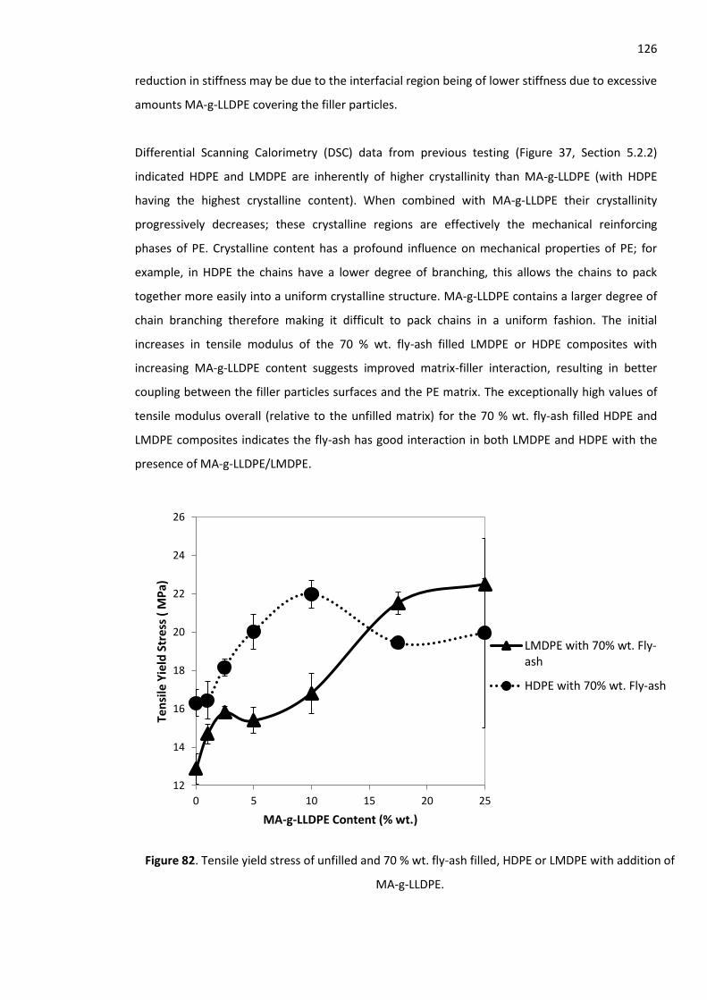
126 reduction in stiffness may be due to the interfacial region being of lower stiffness due to excessive

amounts MA-g-LLDPE covering the filler particles.

Differential Scanning Calorimetry (DSC) data from previous testing (Figure 37, Section 5.2.2)

indicated HDPE and LMDPE are inherently of higher crystallinity than MA-g-LLDPE (with HDPE

having the highest crystalline content). When combined with MA-g-LLDPE their crystallinity

progressively decreases; these crystalline regions are effectively the mechanical reinforcing

phases of PE. Crystalline content has a profound influence on mechanical properties of PE; for

example, in HDPE the chains have a lower degree of branching, this allows the chains to pack

together more easily into a uniform crystalline structure. MA-g-LLDPE contains a larger degree of

chain branching therefore making it difficult to pack chains in a uniform fashion. The initial

increases in tensile modulus of the 70 % wt. fly-ash filled LMDPE or HDPE composites with

increasing MA-g-LLDPE content suggests improved matrix-filler interaction, resulting in better

coupling between the filler particles surfaces and the PE matrix. The exceptionally high values of

tensile modulus overall (relative to the unfilled matrix) for the 70 % wt. fly-ash filled HDPE and

LMDPE composites indicates the fly-ash has good interaction in both LMDPE and HDPE with the

presence of MA-g-LLDPE/LMDPE.

Figure 82. Tensile yield stress of unfilled and 70 % wt. fly-ash filled, HDPE or LMDPE with addition of

MA-g-LLDPE.

12

14

16

18

20

22

24

26

0 5 10 15 20 25

Ten

sile

Yie

ld S

tres

s (

MP

a)

MA-g-LLDPE Content (% wt.)

LMDPE with 70% wt. Fly-ash

HDPE with 70% wt. Fly-ash

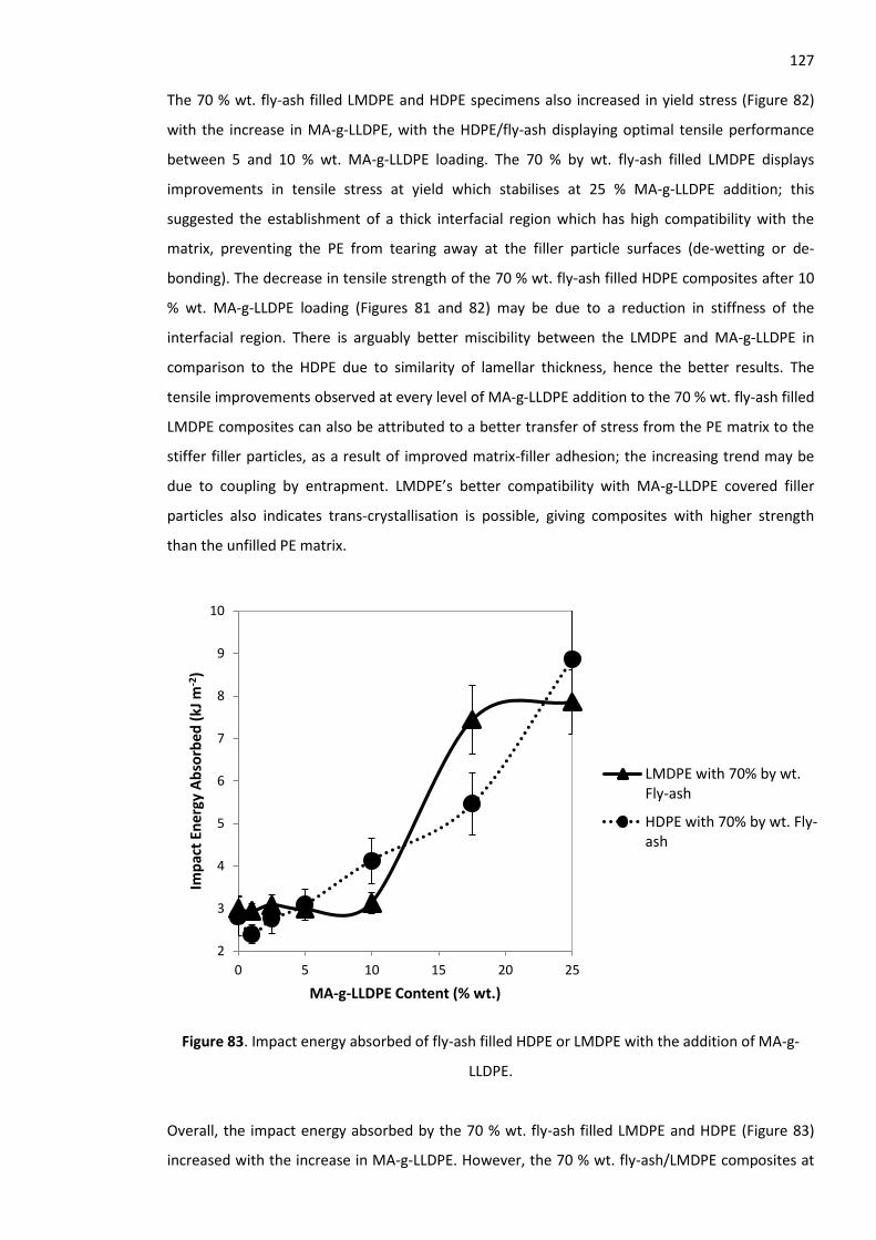
127 The 70 % wt. fly-ash filled LMDPE and HDPE specimens also increased in yield stress (Figure 82)

with the increase in MA-g-LLDPE, with the HDPE/fly-ash displaying optimal tensile performance

between 5 and 10 % wt. MA-g-LLDPE loading. The 70 % by wt. fly-ash filled LMDPE displays

improvements in tensile stress at yield which stabilises at 25 % MA-g-LLDPE addition; this

suggested the establishment of a thick interfacial region which has high compatibility with the

matrix, preventing the PE from tearing away at the filler particle surfaces (de-wetting or de-

bonding). The decrease in tensile strength of the 70 % wt. fly-ash filled HDPE composites after 10

% wt. MA-g-LLDPE loading (Figures 81 and 82) may be due to a reduction in stiffness of the

interfacial region. There is arguably better miscibility between the LMDPE and MA-g-LLDPE in

comparison to the HDPE due to similarity of lamellar thickness, hence the better results. The

tensile improvements observed at every level of MA-g-LLDPE addition to the 70 % wt. fly-ash filled

LMDPE composites can also be attributed to a better transfer of stress from the PE matrix to the

stiffer filler particles, as a result of improved matrix-filler adhesion; the increasing trend may be

due to coupling by entrapment. LMDPE’s better compatibility with MA-g-LLDPE covered filler

particles also indicates trans-crystallisation is possible, giving composites with higher strength

than the unfilled PE matrix.

Figure 83. Impact energy absorbed of fly-ash filled HDPE or LMDPE with the addition of MA-g-

LLDPE.

Overall, the impact energy absorbed by the 70 % wt. fly-ash filled LMDPE and HDPE (Figure 83)

increased with the increase in MA-g-LLDPE. However, the 70 % wt. fly-ash/LMDPE composites at

2

3

4

5

6

7

8

9

10

0 5 10 15 20 25

Imp

act

Ener

gy A

bso

rbe

d (

kJ m

-2)

MA-g-LLDPE Content (% wt.)

LMDPE with 70% by wt.Fly-ash

HDPE with 70% by wt. Fly-ash

128 and beyond 10 % wt. MA-g-LLDPE have a sharper increase in impact properties relative to

equivalent HDPE composites, probably due to greater similarity of lamellar thicknesses. The

increase in impact strength of polymer composites with the presence of MA is not surprising; Kord

[242] observed an increase in the impact strength and tensile properties of PP/wood fibre

composites with increasing levels of MA (up to 2 % wt.). The latter result is remarkable

considering the brittleness of PP above its Tg relative to PE. On the other hand, the wood fibres

are of considerably different shape, size and aspect ratio relative to the smaller spherical fly-ash

particles.

5.8.1 Key findings from the comparison of Maleic Anhydride effects on HDPE and LMDPE fly-ash

composites

Varying the level of coupling agent to assess its effect on the properties particulate-filled polymer

composites for rotational moulding forms another novel aspect of this research. For the purpose

of clarity, the key findings of this investigation are summarised in the following bullet points:

With regards to tensile modulus, the 70 % wt. fly-ash filled LMDPE and HDPE specimens

initially responded well to the introduction of MA-g-LLDPE coupling agent, particularly

between 2.5 and 10 % wt. MA-g-LLDPE loading. However, at MA-g-LLDPE levels exceeding

10 % wt. in 70 % wt. fly-ash filled LMDPE or HDPE composites, the tensile modulus

deteriorated with increasing MA-g-LLDPE addition. This reduction in stiffness may be due

to the interfacial region being of lower stiffness due to excessive amounts MA-g-LLDPE

covering the filler particles.

The exceptionally high values of tensile modulus overall (relative to the unfilled matrix)

for the 70 % wt. fly-ash filled HDPE and LMDPE composites indicates the fly-ash has good

interaction in both LMDPE and HDPE with the presence of MA-g-LLDPE/LMDPE.

The 70 % wt. fly-ash filled HDPE specimens increased in yield stress with the increase in

MA-g-LLDPE, displaying optimal tensile performance between 5 and 10 % wt. MA-g-LLDPE

loading. The decrease in tensile strength of the 70 % wt. fly-ash filled HDPE composites

after 10 % wt. MA-g-LLDPE loading may be due to a reduction in stiffness of the interfacial

region.

The 70 % by wt. fly-ash filled LMDPE displays improvements in tensile stress at yield which

stabilises at 25 % MA-g-LLDPE addition; this suggested the establishment of a thick

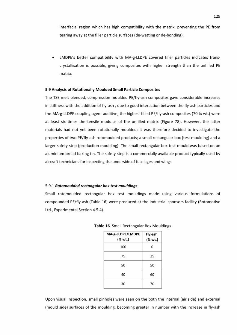
129

interfacial region which has high compatibility with the matrix, preventing the PE from

tearing away at the filler particle surfaces (de-wetting or de-bonding).

LMDPE’s better compatibility with MA-g-LLDPE covered filler particles indicates trans-

crystallisation is possible, giving composites with higher strength than the unfilled PE

matrix.

5.9 Analysis of Rotationally Moulded Small Particle Composites

The TSE melt blended, compression moulded PE/fly-ash composites gave considerable increases

in stiffness with the addition of fly-ash , due to good interaction between the fly-ash particles and

the MA-g-LLDPE coupling agent additive; the highest filled PE/fly-ash composites (70 % wt.) were

at least six times the tensile modulus of the unfilled matrix (Figure 78). However, the latter

materials had not yet been rotationally moulded; it was therefore decided to investigate the

properties of two PE/fly-ash rotomoulded products; a small rectangular box (test moulding) and a

larger safety step (production moulding). The small rectangular box test mould was based on an

aluminium bread baking tin. The safety step is a commercially available product typically used by

aircraft technicians for inspecting the underside of fuselages and wings.

5.9.1 Rotomoulded rectangular box test mouldings

Small rotomoulded rectangular box test mouldings made using various formulations of

compounded PE/fly-ash (Table 16) were produced at the industrial sponsors facility (Rotomotive

Ltd., Experimental Section 4.5.4).

Table 16. Small Rectangular Box Mouldings

MA-g-LLDPE/LMDPE

(% wt.) Fly-ash. (% wt.)

100 0

75 25

50 50

40 60

30 70

Upon visual inspection, small pinholes were seen on the both the internal (air side) and external

(mould side) surfaces of the moulding, becoming greater in number with the increase in fly-ash

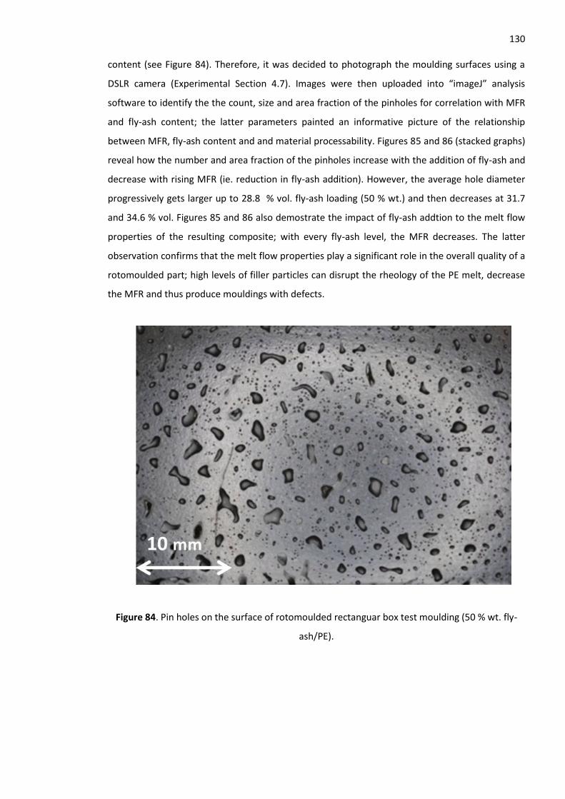
130 content (see Figure 84). Therefore, it was decided to photograph the moulding surfaces using a

DSLR camera (Experimental Section 4.7). Images were then uploaded into “imageJ” analysis

software to identify the the count, size and area fraction of the pinholes for correlation with MFR

and fly-ash content; the latter parameters painted an informative picture of the relationship

between MFR, fly-ash content and and material processability. Figures 85 and 86 (stacked graphs)

reveal how the number and area fraction of the pinholes increase with the addition of fly-ash and

decrease with rising MFR (ie. reduction in fly-ash addition). However, the average hole diameter

progressively gets larger up to 28.8 % vol. fly-ash loading (50 % wt.) and then decreases at 31.7

and 34.6 % vol. Figures 85 and 86 also demostrate the impact of fly-ash addtion to the melt flow

properties of the resulting composite; with every fly-ash level, the MFR decreases. The latter

observation confirms that the melt flow properties play a significant role in the overall quality of a

rotomoulded part; high levels of filler particles can disrupt the rheology of the PE melt, decrease

the MFR and thus produce mouldings with defects.

Figure 84. Pin holes on the surface of rotomoulded rectanguar box test moulding (50 % wt. fly-

ash/PE).

131

Figure 85. Pinhole count, area fraction and diameter vs. MFR of MA-g-LLDPE/LMDPE with fly-ash.

0

500

1000

1500

2000

2500

3000

Nu

mb

er

of

Po

rou

s H

ole

s o

n S

urf

ace

0

2

4

6

8

10

12

Are

a Fr

acti

on

of

Po

rou

s H

ole

s

0

0.1

0.2

0.3

0.4

0.5

0.6

0.5 1 1.5 2 2.5 3 3.5

Ave

rage

Po

rou

s H

ole

Dia

met

er

(m

m)

Melt Flow Rate (dg min-1)

132

Figure 86. Pinhole count, area fraction and diameter vs. fly-ash content in MA-g-LLDPE/LMDPE.

0

500

1000

1500

2000

2500

3000

Nu

mb

er

of

Po

rou

s H

ole

s o

n S

urf

ace

0

2

4

6

8

10

12

Are

a Fr

acti

on

of

Po

rou

s H

ole

s

0

0.1

0.2

0.3

0.4

0.5

0.6

0 5 10 15 20 25 30 35 40

Ave

rage

Po

rou

s H

ole

Dia

met

er

(m

m)

Fly-ash content (% vol.)

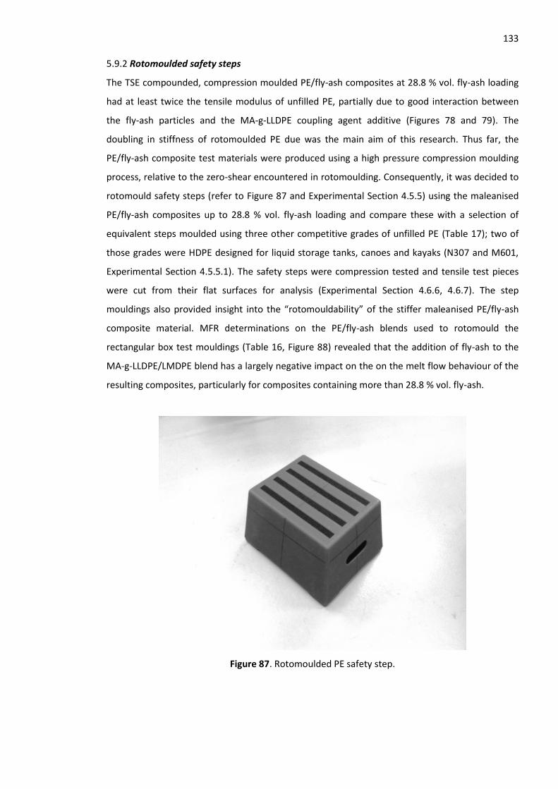
133 5.9.2 Rotomoulded safety steps

The TSE compounded, compression moulded PE/fly-ash composites at 28.8 % vol. fly-ash loading

had at least twice the tensile modulus of unfilled PE, partially due to good interaction between

the fly-ash particles and the MA-g-LLDPE coupling agent additive (Figures 78 and 79). The

doubling in stiffness of rotomoulded PE due was the main aim of this research. Thus far, the

PE/fly-ash composite test materials were produced using a high pressure compression moulding

process, relative to the zero-shear encountered in rotomoulding. Consequently, it was decided to

rotomould safety steps (refer to Figure 87 and Experimental Section 4.5.5) using the maleanised

PE/fly-ash composites up to 28.8 % vol. fly-ash loading and compare these with a selection of

equivalent steps moulded using three other competitive grades of unfilled PE (Table 17); two of

those grades were HDPE designed for liquid storage tanks, canoes and kayaks (N307 and M601,

Experimental Section 4.5.5.1). The safety steps were compression tested and tensile test pieces

were cut from their flat surfaces for analysis (Experimental Section 4.6.6, 4.6.7). The step

mouldings also provided insight into the “rotomouldability” of the stiffer maleanised PE/fly-ash

composite material. MFR determinations on the PE/fly-ash blends used to rotomould the

rectangular box test mouldings (Table 16, Figure 88) revealed that the addition of fly-ash to the

MA-g-LLDPE/LMDPE blend has a largely negative impact on the on the melt flow behaviour of the

resulting composites, particularly for composites containing more than 28.8 % vol. fly-ash.

Figure 87. Rotomoulded PE safety step.

134

Table 17. Unfilled PE grades used for rotomoulded safety steps.

Table 18. PE/fly-ash formulations for rotomoulded safety steps.

Target Wall Thickness (mm)

MA-g-LLDPE/LMDPE (% wt.)

Fly-ash (% vol.)

Fly-ash (% wt.)

7 50 28.8 50

7 75 14.4 25

7 87.5 7.2 12.5

7 100 0 0

Figure 88. MFR of MA-g-LLDPE/LMDPE with the addition of fly-ash, specified in Table 16.

Liquid displacement and ashing tests were also conducted (Figure 89) in order to determine the

density of the PE/fly-ash composites (Experimental Section 4.3.5); the ashing type test provided a

pinpoint accurate verification of the filler content due to combustion of the polymer within the

composite, leaving the fly-ash residue.

0

0.5

1

1.5

2

2.5

3

3.5

4

0 10 20 30 40

Mel

t Fl

ow

Rat

e (d

g m

in-1

)

Fly-ash Content (% vol.)

Target Wall Thickness (mm)

PE Grade

7 N-250 LMDPE

7 N-307 HDPE

7 M-601 HDPE

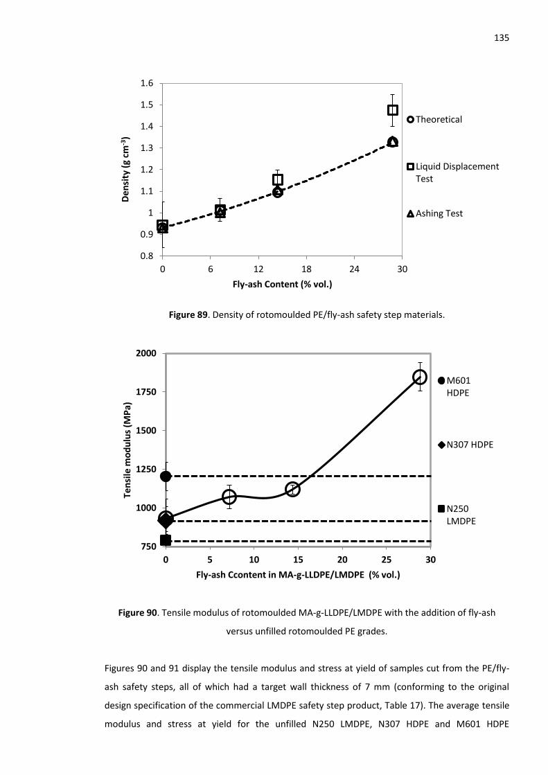
135

Figure 89. Density of rotomoulded PE/fly-ash safety step materials.

Figure 90. Tensile modulus of rotomoulded MA-g-LLDPE/LMDPE with the addition of fly-ash

versus unfilled rotomoulded PE grades.

Figures 90 and 91 display the tensile modulus and stress at yield of samples cut from the PE/fly-

ash safety steps, all of which had a target wall thickness of 7 mm (conforming to the original

design specification of the commercial LMDPE safety step product, Table 17). The average tensile

modulus and stress at yield for the unfilled N250 LMDPE, N307 HDPE and M601 HDPE

0.8

0.9

1

1.1

1.2

1.3

1.4

1.5

1.6

0 6 12 18 24 30

De

nsi

ty (

g cm

-3)

Fly-ash Content (% vol.)

Theoretical

Liquid DisplacementTest

Ashing Test

750

1000

1250

1500

1750

2000

0 5 10 15 20 25 30

Ten

sile

mo

du

lus

(MP

a)

Fly-ash Ccontent in MA-g-LLDPE/LMDPE (% vol.)

M601HDPE

N307 HDPE

N250LMDPE

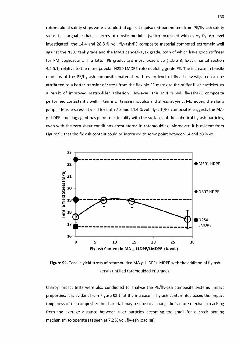
136 rotomoulded safety steps were also plotted against equivalent parameters from PE/fly-ash safety

steps. It is arguable that, in terms of tensile modulus (which increased with every fly-ash level

investigated) the 14.4 and 28.8 % vol. fly-ash/PE composite material competed extremely well

against the N307 tank grade and the M601 canoe/kayak grade, both of which have good stiffness

for RM applications. The latter PE grades are more expensive (Table 3, Experimental section

4.5.5.1) relative to the more popular N250 LMDPE rotomoulding grade PE. The increase in tensile

modulus of the PE/fly-ash composite materials with every level of fly-ash investigated can be

attributed to a better transfer of stress from the flexible PE matrix to the stiffer filler particles, as

a result of improved matrix-filler adhesion. However, the 14.4 % vol. fly-ash/PE composite

performed consistently well in terms of tensile modulus and stress at yield. Moreover, the sharp

jump in tensile stress at yield for both 7.2 and 14.4 % vol. fly-ash/PE composites suggests the MA-

g-LLDPE coupling agent has good functionality with the surfaces of the spherical fly-ash particles,

even with the zero-shear conditions encountered in rotomoulding. Moreover, it is evident from

Figure 91 that the fly-ash content could be increased to some point between 14 and 28 % vol.

Figure 91. Tensile yield stress of rotomoulded MA-g-LLDPE/LMDPE with the addition of fly-ash

versus unfilled rotomoulded PE grades.

Charpy impact tests were also conducted to analyse the PE/fly-ash composite systems impact

properties. It is evident from Figure 92 that the increase in fly-ash content decreases the impact

toughness of the composite; the sharp fall may be due to a change in fracture mechanism arising

from the average distance between filler particles becoming too small for a crack pinning

mechanism to operate (as seen at 7.2 % vol. fly-ash loading).

16

17

18

19

20

21

22

23

0 5 10 15 20 25 30

Ten

sile

Yie

ld S

tre

ss (

MP

a)

Fly-ash Content in MA-g-LLDPE/LMDPE (% vol.)

M601 HDPE

N307 HDPE

N250LMDPE

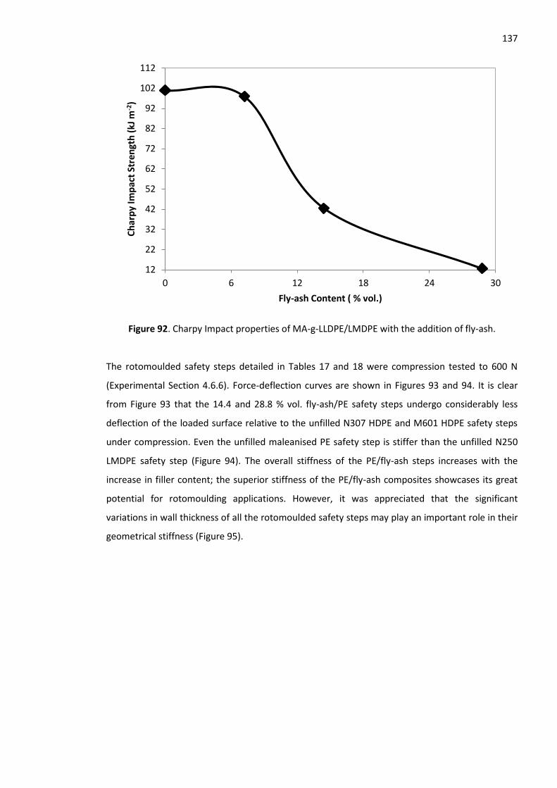
137

Figure 92. Charpy Impact properties of MA-g-LLDPE/LMDPE with the addition of fly-ash.

The rotomoulded safety steps detailed in Tables 17 and 18 were compression tested to 600 N

(Experimental Section 4.6.6). Force-deflection curves are shown in Figures 93 and 94. It is clear

from Figure 93 that the 14.4 and 28.8 % vol. fly-ash/PE safety steps undergo considerably less

deflection of the loaded surface relative to the unfilled N307 HDPE and M601 HDPE safety steps

under compression. Even the unfilled maleanised PE safety step is stiffer than the unfilled N250

LMDPE safety step (Figure 94). The overall stiffness of the PE/fly-ash steps increases with the

increase in filler content; the superior stiffness of the PE/fly-ash composites showcases its great

potential for rotomoulding applications. However, it was appreciated that the significant

variations in wall thickness of all the rotomoulded safety steps may play an important role in their

geometrical stiffness (Figure 95).

12

22

32

42

52

62

72

82

92

102

112

0 6 12 18 24 30

Ch

arp

y Im

pac

t St

ren

gth

(kJ

m-2

)

Fly-ash Content ( % vol.)

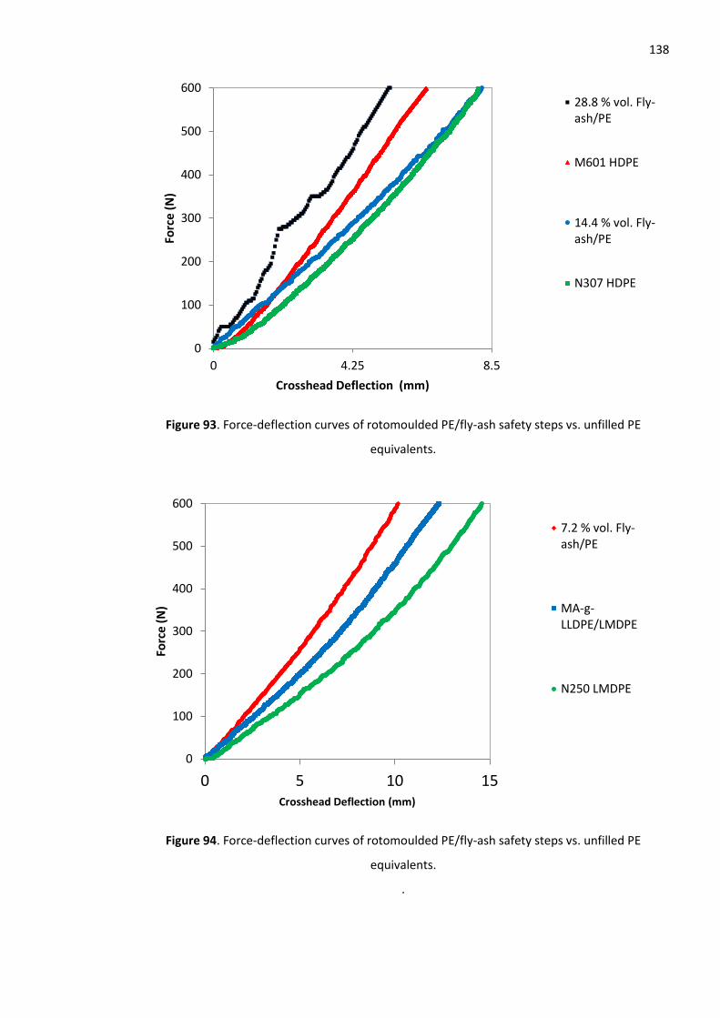
138

Figure 93. Force-deflection curves of rotomoulded PE/fly-ash safety steps vs. unfilled PE

equivalents.

Figure 94. Force-deflection curves of rotomoulded PE/fly-ash safety steps vs. unfilled PE

equivalents.

.

0

100

200

300

400

500

600

0 4.25 8.5

Forc

e (N

)

Crosshead Deflection (mm)

28.8 % vol. Fly-ash/PE

M601 HDPE

14.4 % vol. Fly-ash/PE

N307 HDPE

0

100

200

300

400

500

600

0 5 10 15

Forc

e (N

)

Crosshead Deflection (mm)

7.2 % vol. Fly-ash/PE

MA-g-LLDPE/LMDPE

N250 LMDPE

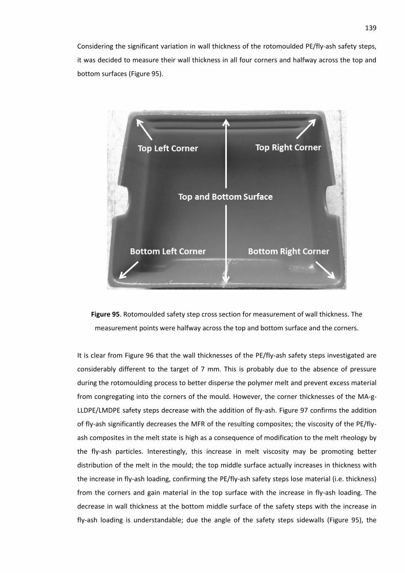
139 Considering the significant variation in wall thickness of the rotomoulded PE/fly-ash safety steps,

it was decided to measure their wall thickness in all four corners and halfway across the top and

bottom surfaces (Figure 95).

Figure 95. Rotomoulded safety step cross section for measurement of wall thickness. The

measurement points were halfway across the top and bottom surface and the corners.

It is clear from Figure 96 that the wall thicknesses of the PE/fly-ash safety steps investigated are

considerably different to the target of 7 mm. This is probably due to the absence of pressure

during the rotomoulding process to better disperse the polymer melt and prevent excess material

from congregating into the corners of the mould. However, the corner thicknesses of the MA-g-

LLDPE/LMDPE safety steps decrease with the addition of fly-ash. Figure 97 confirms the addition

of fly-ash significantly decreases the MFR of the resulting composites; the viscosity of the PE/fly-

ash composites in the melt state is high as a consequence of modification to the melt rheology by

the fly-ash particles. Interestingly, this increase in melt viscosity may be promoting better

distribution of the melt in the mould; the top middle surface actually increases in thickness with

the increase in fly-ash loading, confirming the PE/fly-ash safety steps lose material (i.e. thickness)

from the corners and gain material in the top surface with the increase in fly-ash loading. The

decrease in wall thickness at the bottom middle surface of the safety steps with the increase in

fly-ash loading is understandable; due the angle of the safety steps sidewalls (Figure 95), the

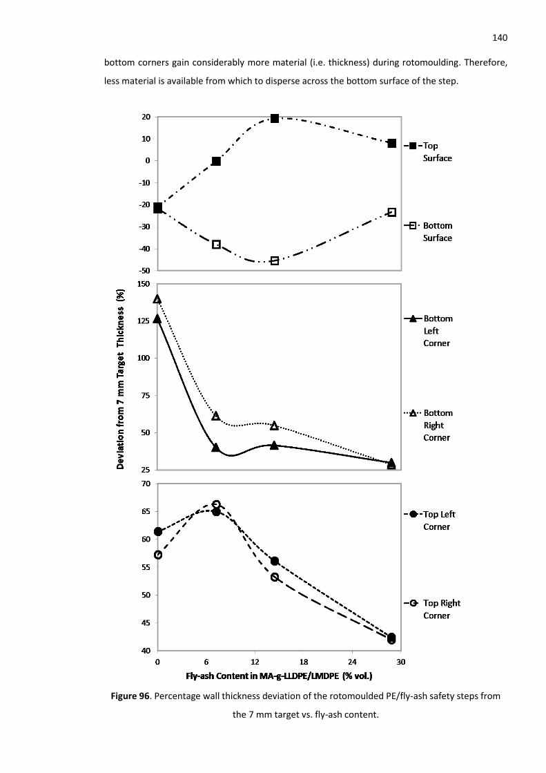
140 bottom corners gain considerably more material (i.e. thickness) during rotomoulding. Therefore,

less material is available from which to disperse across the bottom surface of the step.

Figure 96. Percentage wall thickness deviation of the rotomoulded PE/fly-ash safety steps from

the 7 mm target vs. fly-ash content.

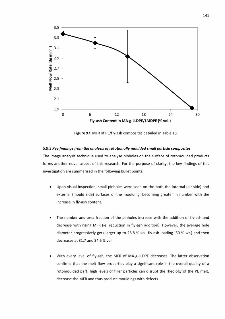
141

Figure 97. MFR of PE/fly-ash composites detailed in Table 18.

5.9.3 Key findings from the analysis of rotationally moulded small particle composites

The image analysis technique used to analyse pinholes on the surface of rotomoulded products

forms another novel aspect of this research. For the purpose of clarity, the key findings of this

investigation are summarised in the following bullet points:

Upon visual inspection, small pinholes were seen on the both the internal (air side) and

external (mould side) surfaces of the moulding, becoming greater in number with the

increase in fly-ash content.

The number and area fraction of the pinholes increase with the addition of fly-ash and

decrease with rising MFR (ie. reduction in fly-ash addition). However, the average hole

diameter progressively gets larger up to 28.8 % vol. fly-ash loading (50 % wt.) and then

decreases at 31.7 and 34.6 % vol.

With every level of fly-ash, the MFR of MA-g-LLDPE decreases. The latter observation

confirms that the melt flow properties play a significant role in the overall quality of a

rotomoulded part; high levels of filler particles can disrupt the rheology of the PE melt,

decrease the MFR and thus produce mouldings with defects.

1.9

2.1

2.3

2.5

2.7

2.9

3.1

3.3

3.5

0 6 12 18 24 30

Mel

t Fl

ow

Rat

e (d

g m

in.-

1)

Fly-ash Content in MA-g-LLDPE/LMDPE (% vol.)

142

In terms of tensile modulus (which increased with every fly-ash level investigated) the

14.4 and 28.8 % vol. fly-ash/PE composite material competed extremely well against the

N307 tank grade and the M601 canoe/kayak grade, both of which have good stiffness for

RM applications.

The 14.4 % vol. fly-ash/PE composite performed consistently well in terms of tensile

modulus and stress at yield. Moreover, the sharp jump in tensile stress at yield for both

7.2 and 14.4 % vol. fly-ash/PE composites suggests the MA-g-LLDPE coupling agent has

good functionality with the surfaces of the spherical fly-ash particles, even with the zero-

shear conditions encountered in rotomoulding.

It is evident that the fly-ash content could be increased to some point between 14 and 28

% vol. in an effort to balance the increase in modulus with better impact properties.

The increase in fly-ash content decreases the impact toughness of the composite; the

sharp fall may be due to a change in fracture mechanism arising from the average

distance between filler particles becoming too small for a crack pinning mechanism to

operate (as seen at 7.2 % vol. fly-ash loading).

The 14.4 and 28.8 % vol. fly-ash/PE safety steps undergo considerably less deflection of

the loaded surface relative to the unfilled N307 HDPE and M601 HDPE safety steps under

compression.

The unfilled MA-g-LLDPE safety step is stiffer than the unfilled N250 LMDPE safety step.

However, the overall stiffness of the PE/fly-ash steps increases with the increase in filler

content; the superior stiffness of the PE/fly-ash composites showcases its great potential

for rotomoulding applications.

The viscosity of the PE/fly-ash composites in the melt state is high as a consequence of

modification to the melt rheology by the fly-ash particles. Interestingly, this increase in

melt viscosity may be promoting better distribution of the melt in the mould.

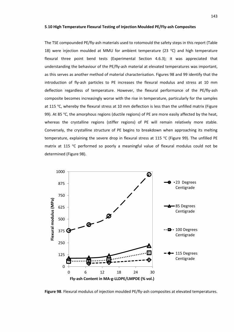
143 5.10 High Temperature Flexural Testing of Injection Moulded PE/Fly-ash Composites

The TSE compounded PE/fly-ash materials used to rotomould the safety steps in this report (Table

18) were injection moulded at MMU for ambient temperature (23 oC) and high temperature

flexural three point bend tests (Experimental Section 4.6.3); it was appreciated that

understanding the behaviour of the PE/fly-ash material at elevated temperatures was important,

as this serves as another method of material characterisation. Figures 98 and 99 identify that the

introduction of fly-ash particles to PE increases the flexural modulus and stress at 10 mm

deflection regardless of temperature. However, the flexural performance of the PE/fly-ash

composite becomes increasingly worse with the rise in temperature, particularly for the samples

at 115 oC, whereby the flexural stress at 10 mm deflection is less than the unfilled matrix (Figure

99). At 85 oC, the amorphous regions (ductile regions) of PE are more easily affected by the heat,

whereas the crystalline regions (stiffer regions) of PE will remain relatively more stable.

Conversely, the crystalline structure of PE begins to breakdown when approaching its melting

temperature, explaining the severe drop in flexural stress at 115 oC (Figure 99). The unfilled PE

matrix at 115 oC performed so poorly a meaningful value of flexural modulus could not be

determined (Figure 98).

Figure 98. Flexural modulus of injection moulded PE/fly-ash composites at elevated temperatures.

0

125

250

375

500

625

750

875

1000

0 6 12 18 24 30

Fle

xura

l mo

du

lus

(MP

a)

Fly-ash Content in MA-g-LLDPE/LMPDE (% vol.)

23 DegreesCentigrade

85 DegreesCentigrade

100 DegreesCentigrade

115 DegreesCentigrade

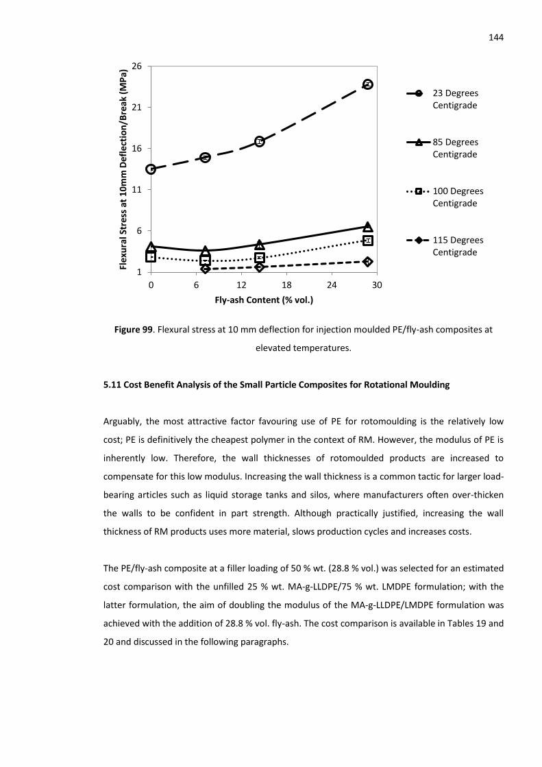
144

Figure 99. Flexural stress at 10 mm deflection for injection moulded PE/fly-ash composites at

elevated temperatures.

5.11 Cost Benefit Analysis of the Small Particle Composites for Rotational Moulding

Arguably, the most attractive factor favouring use of PE for rotomoulding is the relatively low

cost; PE is definitively the cheapest polymer in the context of RM. However, the modulus of PE is

inherently low. Therefore, the wall thicknesses of rotomoulded products are increased to

compensate for this low modulus. Increasing the wall thickness is a common tactic for larger load-

bearing articles such as liquid storage tanks and silos, where manufacturers often over-thicken

the walls to be confident in part strength. Although practically justified, increasing the wall

thickness of RM products uses more material, slows production cycles and increases costs.

The PE/fly-ash composite at a filler loading of 50 % wt. (28.8 % vol.) was selected for an estimated

cost comparison with the unfilled 25 % wt. MA-g-LLDPE/75 % wt. LMDPE formulation; with the

latter formulation, the aim of doubling the modulus of the MA-g-LLDPE/LMDPE formulation was

achieved with the addition of 28.8 % vol. fly-ash. The cost comparison is available in Tables 19 and

20 and discussed in the following paragraphs.

1

6

11

16

21

26

0 6 12 18 24 30

Fle

xura

l Str

ess

at 1

0m

m D

efl

ecti

on

/Bre

ak (

MP

a)

Fly-ash Content (% vol.)

23 DegreesCentigrade

85 DegreesCentigrade

100 DegreesCentigrade

115 DegreesCentigrade

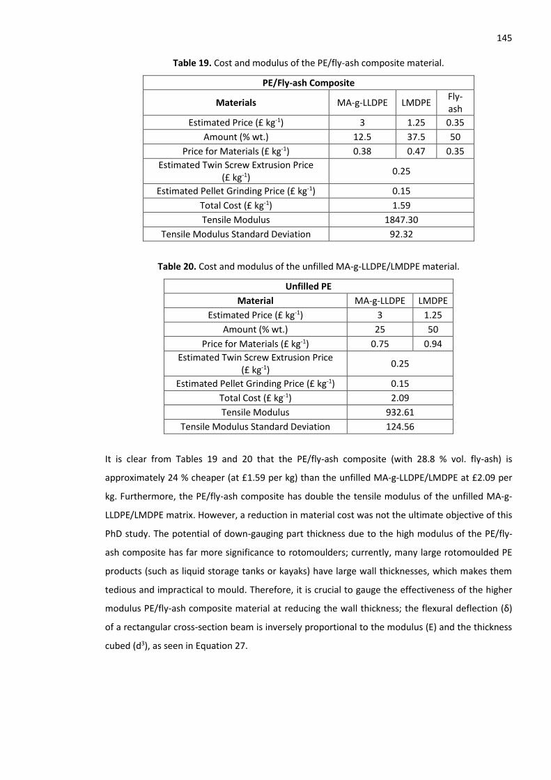
145

Table 19. Cost and modulus of the PE/fly-ash composite material.

PE/Fly-ash Composite

Materials MA-g-LLDPE LMDPE Fly-ash

Estimated Price (£ kg-1) 3 1.25 0.35

Amount (% wt.) 12.5 37.5 50

Price for Materials (£ kg-1) 0.38 0.47 0.35

Estimated Twin Screw Extrusion Price (£ kg-1)

0.25

Estimated Pellet Grinding Price (£ kg-1) 0.15

Total Cost (£ kg-1) 1.59

Tensile Modulus 1847.30

Tensile Modulus Standard Deviation 92.32

Table 20. Cost and modulus of the unfilled MA-g-LLDPE/LMDPE material.

Unfilled PE

Material MA-g-LLDPE LMDPE

Estimated Price (£ kg-1) 3 1.25

Amount (% wt.) 25 50

Price for Materials (£ kg-1) 0.75 0.94

Estimated Twin Screw Extrusion Price (£ kg-1)

0.25

Estimated Pellet Grinding Price (£ kg-1) 0.15

Total Cost (£ kg-1) 2.09

Tensile Modulus 932.61

Tensile Modulus Standard Deviation 124.56

It is clear from Tables 19 and 20 that the PE/fly-ash composite (with 28.8 % vol. fly-ash) is

approximately 24 % cheaper (at £1.59 per kg) than the unfilled MA-g-LLDPE/LMDPE at £2.09 per

kg. Furthermore, the PE/fly-ash composite has double the tensile modulus of the unfilled MA-g-

LLDPE/LMDPE matrix. However, a reduction in material cost was not the ultimate objective of this

PhD study. The potential of down-gauging part thickness due to the high modulus of the PE/fly-

ash composite has far more significance to rotomoulders; currently, many large rotomoulded PE

products (such as liquid storage tanks or kayaks) have large wall thicknesses, which makes them

tedious and impractical to mould. Therefore, it is crucial to gauge the effectiveness of the higher

modulus PE/fly-ash composite material at reducing the wall thickness; the flexural deflection (δ)

of a rectangular cross-section beam is inversely proportional to the modulus (E) and the thickness

cubed (d3), as seen in Equation 27.

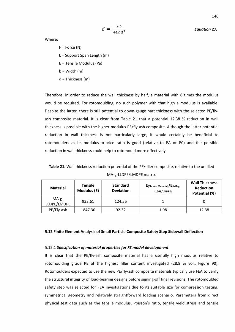
146

𝛿 = 𝐹𝐿

4𝐸𝑏𝑑3 Equation 27.

Where:

F = Force (N)

L = Support Span Length (m)

E = Tensile Modulus (Pa)

b = Width (m)

d = Thickness (m)

Therefore, in order to reduce the wall thickness by half, a material with 8 times the modulus

would be required. For rotomoulding, no such polymer with that high a modulus is available.

Despite the latter, there is still potential to down-gauge part thickness with the selected PE/fly-

ash composite material. It is clear from Table 21 that a potential 12.38 % reduction in wall

thickness is possible with the higher modulus PE/fly-ash composite. Although the latter potential

reduction in wall thickness is not particularly large, it would certainly be beneficial to

rotomoulders as its modulus-to-price ratio is good (relative to PA or PC) and the possible

reduction in wall thickness could help to rotomould more effectively.

Table 21. Wall thickness reduction potential of the PE/filler composite, relative to the unfilled

MA-g-LLDPE/LMDPE matrix.

Material Tensile

Modulus (E) Standard Deviation

E(Chosen Material)/E(MA-g-

LLDPE/LMDPE)

Wall Thickness Reduction

Potential (%)

MA-g-LLDPE/LMDPE

932.61 124.56 1 0

PE/Fly-ash 1847.30 92.32 1.98 12.38

5.12 Finite Element Analysis of Small Particle Composite Safety Step Sidewall Deflection

5.12.1 Specification of material properties for FE model development

It is clear that the PE/fly-ash composite material has a usefully high modulus relative to

rotomoulding grade PE at the highest filler content investigated (28.8 % vol., Figure 90).

Rotomoulders expected to use the new PE/fly-ash composite materials typically use FEA to verify

the structural integrity of load-bearing designs before signing-off final revisions. The rotomoulded

safety step was selected for FEA investigations due to its suitable size for compression testing,

symmetrical geometry and relatively straightforward loading scenario. Parameters from direct

physical test data such as the tensile modulus, Poisson’s ratio, tensile yield stress and tensile

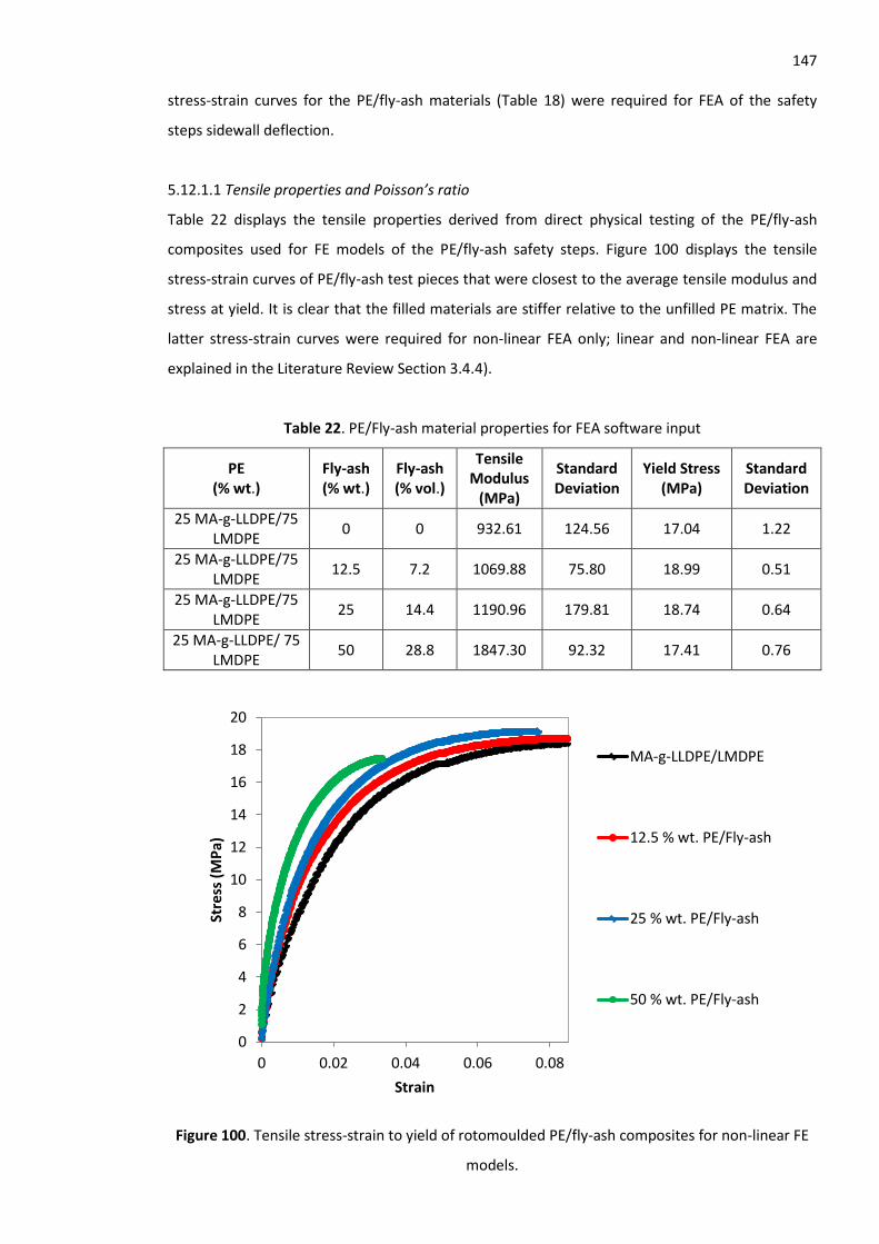
147 stress-strain curves for the PE/fly-ash materials (Table 18) were required for FEA of the safety

steps sidewall deflection.

5.12.1.1 Tensile properties and Poisson’s ratio

Table 22 displays the tensile properties derived from direct physical testing of the PE/fly-ash

composites used for FE models of the PE/fly-ash safety steps. Figure 100 displays the tensile

stress-strain curves of PE/fly-ash test pieces that were closest to the average tensile modulus and

stress at yield. It is clear that the filled materials are stiffer relative to the unfilled PE matrix. The

latter stress-strain curves were required for non-linear FEA only; linear and non-linear FEA are

explained in the Literature Review Section 3.4.4).

Table 22. PE/Fly-ash material properties for FEA software input

PE (% wt.)

Fly-ash (% wt.)

Fly-ash (% vol.)

Tensile Modulus

(MPa)

Standard Deviation

Yield Stress (MPa)

Standard Deviation

25 MA-g-LLDPE/75 LMDPE

0 0 932.61 124.56 17.04 1.22

25 MA-g-LLDPE/75 LMDPE

12.5 7.2 1069.88 75.80 18.99 0.51

25 MA-g-LLDPE/75 LMDPE

25 14.4 1190.96 179.81 18.74 0.64

25 MA-g-LLDPE/ 75 LMDPE

50 28.8 1847.30 92.32 17.41 0.76

Figure 100. Tensile stress-strain to yield of rotomoulded PE/fly-ash composites for non-linear FE

models.

0

2

4

6

8

10

12

14

16

18

20

0 0.02 0.04 0.06 0.08

Stre

ss (

MP

a)

Strain

MA-g-LLDPE/LMDPE

12.5 % wt. PE/Fly-ash

25 % wt. PE/Fly-ash

50 % wt. PE/Fly-ash

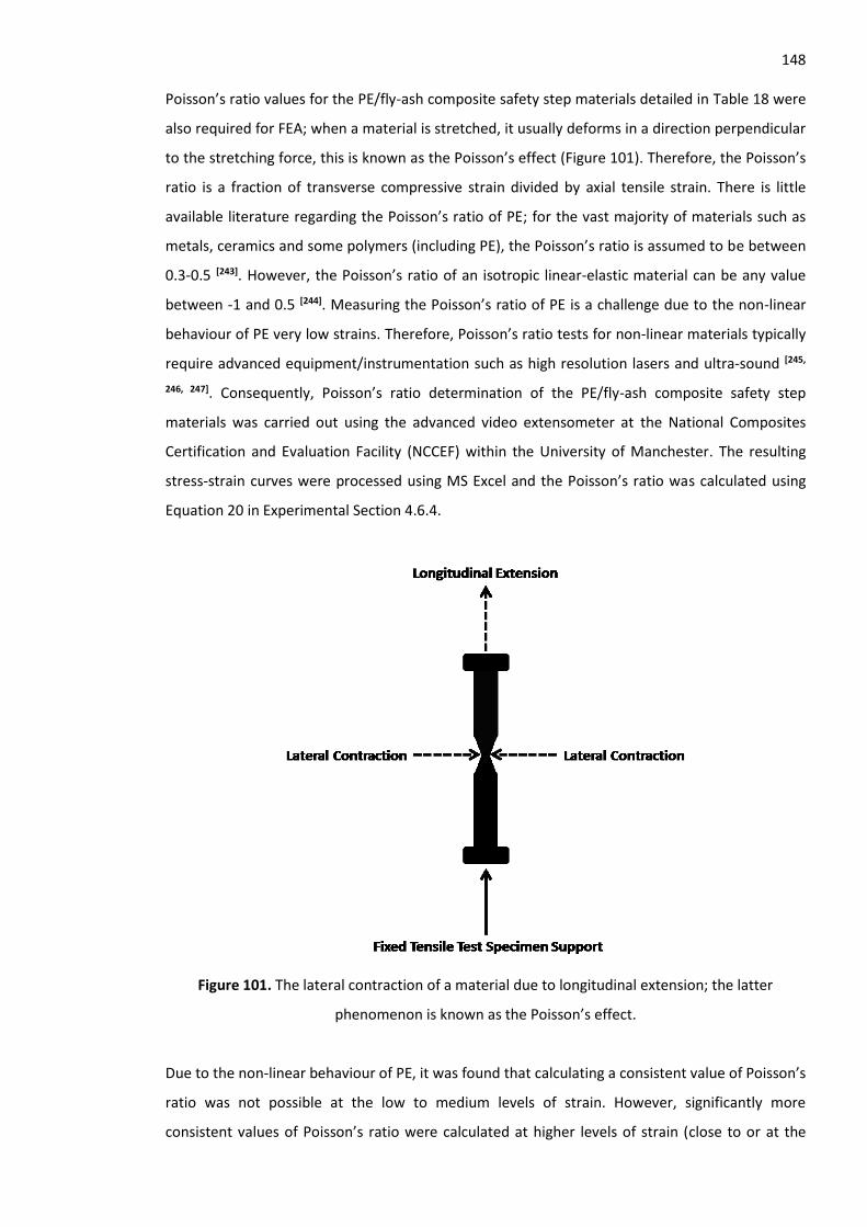
148 Poisson’s ratio values for the PE/fly-ash composite safety step materials detailed in Table 18 were

also required for FEA; when a material is stretched, it usually deforms in a direction perpendicular

to the stretching force, this is known as the Poisson’s effect (Figure 101). Therefore, the Poisson’s

ratio is a fraction of transverse compressive strain divided by axial tensile strain. There is little

available literature regarding the Poisson’s ratio of PE; for the vast majority of materials such as

metals, ceramics and some polymers (including PE), the Poisson’s ratio is assumed to be between

0.3-0.5 [243]. However, the Poisson’s ratio of an isotropic linear-elastic material can be any value

between -1 and 0.5 [244]. Measuring the Poisson’s ratio of PE is a challenge due to the non-linear

behaviour of PE very low strains. Therefore, Poisson’s ratio tests for non-linear materials typically

require advanced equipment/instrumentation such as high resolution lasers and ultra-sound [245,

246, 247]. Consequently, Poisson’s ratio determination of the PE/fly-ash composite safety step

materials was carried out using the advanced video extensometer at the National Composites

Certification and Evaluation Facility (NCCEF) within the University of Manchester. The resulting

stress-strain curves were processed using MS Excel and the Poisson’s ratio was calculated using

Equation 20 in Experimental Section 4.6.4.

Figure 101. The lateral contraction of a material due to longitudinal extension; the latter

phenomenon is known as the Poisson’s effect.

Due to the non-linear behaviour of PE, it was found that calculating a consistent value of Poisson’s

ratio was not possible at the low to medium levels of strain. However, significantly more

consistent values of Poisson’s ratio were calculated at higher levels of strain (close to or at the

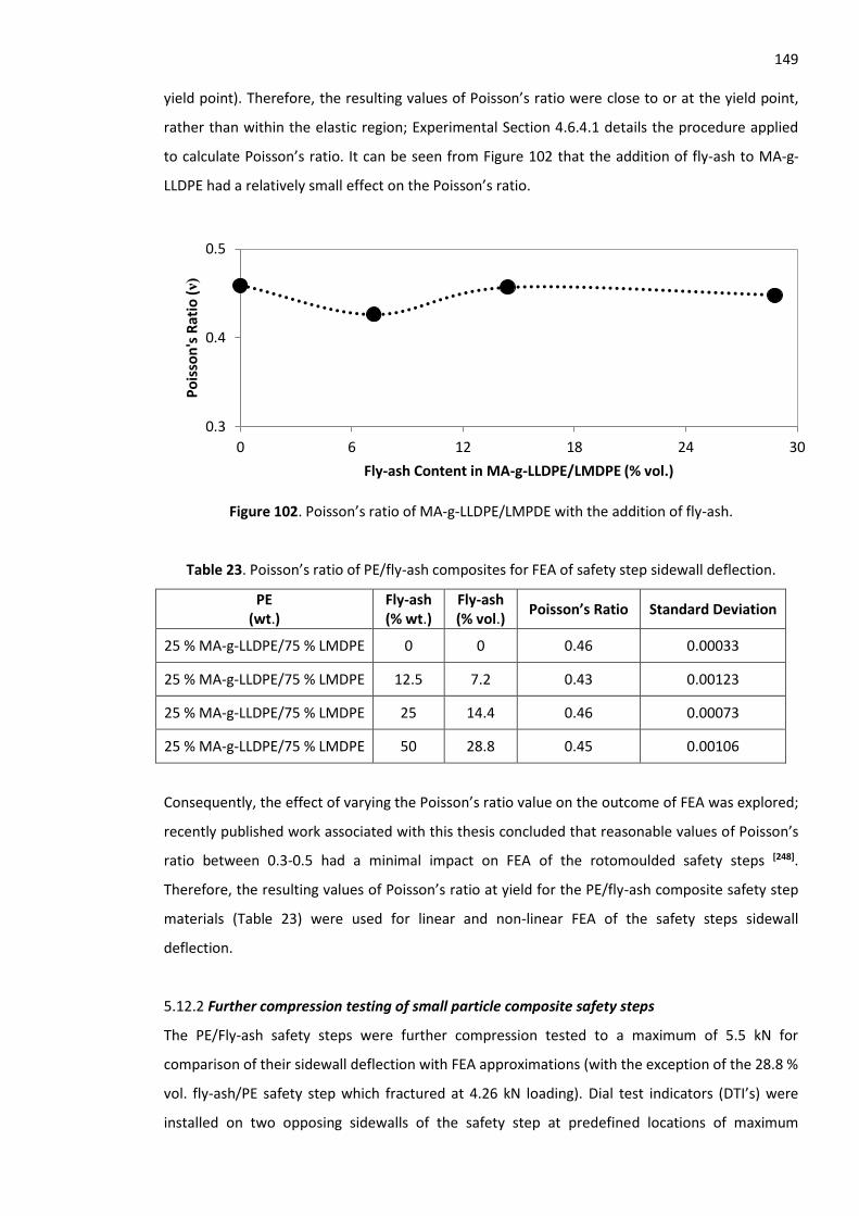
149 yield point). Therefore, the resulting values of Poisson’s ratio were close to or at the yield point,

rather than within the elastic region; Experimental Section 4.6.4.1 details the procedure applied

to calculate Poisson’s ratio. It can be seen from Figure 102 that the addition of fly-ash to MA-g-

LLDPE had a relatively small effect on the Poisson’s ratio.

Figure 102. Poisson’s ratio of MA-g-LLDPE/LMPDE with the addition of fly-ash.

Table 23. Poisson’s ratio of PE/fly-ash composites for FEA of safety step sidewall deflection.

PE (wt.)

Fly-ash (% wt.)

Fly-ash (% vol.)

Poisson’s Ratio Standard Deviation

25 % MA-g-LLDPE/75 % LMDPE 0 0 0.46 0.00033

25 % MA-g-LLDPE/75 % LMDPE 12.5 7.2 0.43 0.00123

25 % MA-g-LLDPE/75 % LMDPE 25 14.4 0.46 0.00073

25 % MA-g-LLDPE/75 % LMDPE 50 28.8 0.45 0.00106

Consequently, the effect of varying the Poisson’s ratio value on the outcome of FEA was explored;

recently published work associated with this thesis concluded that reasonable values of Poisson’s

ratio between 0.3-0.5 had a minimal impact on FEA of the rotomoulded safety steps [248].

Therefore, the resulting values of Poisson’s ratio at yield for the PE/fly-ash composite safety step

materials (Table 23) were used for linear and non-linear FEA of the safety steps sidewall

deflection.

5.12.2 Further compression testing of small particle composite safety steps

The PE/Fly-ash safety steps were further compression tested to a maximum of 5.5 kN for

comparison of their sidewall deflection with FEA approximations (with the exception of the 28.8 %

vol. fly-ash/PE safety step which fractured at 4.26 kN loading). Dial test indicators (DTI’s) were

installed on two opposing sidewalls of the safety step at predefined locations of maximum

0.3

0.4

0.5

0 6 12 18 24 30

Po

isso

n's

Rat

io (ν)

Fly-ash Content in MA-g-LLDPE/LMDPE (% vol.)

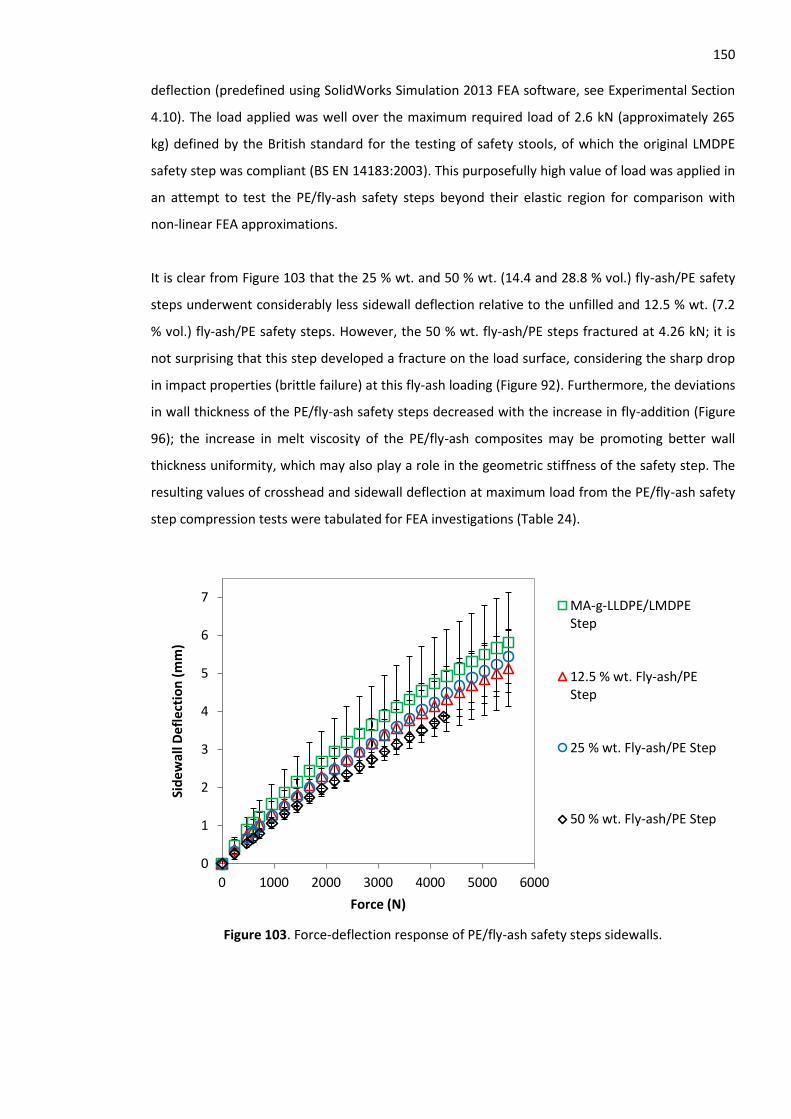
150 deflection (predefined using SolidWorks Simulation 2013 FEA software, see Experimental Section

4.10). The load applied was well over the maximum required load of 2.6 kN (approximately 265

kg) defined by the British standard for the testing of safety stools, of which the original LMDPE

safety step was compliant (BS EN 14183:2003). This purposefully high value of load was applied in

an attempt to test the PE/fly-ash safety steps beyond their elastic region for comparison with

non-linear FEA approximations.

It is clear from Figure 103 that the 25 % wt. and 50 % wt. (14.4 and 28.8 % vol.) fly-ash/PE safety

steps underwent considerably less sidewall deflection relative to the unfilled and 12.5 % wt. (7.2

% vol.) fly-ash/PE safety steps. However, the 50 % wt. fly-ash/PE steps fractured at 4.26 kN; it is

not surprising that this step developed a fracture on the load surface, considering the sharp drop

in impact properties (brittle failure) at this fly-ash loading (Figure 92). Furthermore, the deviations

in wall thickness of the PE/fly-ash safety steps decreased with the increase in fly-addition (Figure

96); the increase in melt viscosity of the PE/fly-ash composites may be promoting better wall

thickness uniformity, which may also play a role in the geometric stiffness of the safety step. The

resulting values of crosshead and sidewall deflection at maximum load from the PE/fly-ash safety

step compression tests were tabulated for FEA investigations (Table 24).

Figure 103. Force-deflection response of PE/fly-ash safety steps sidewalls.

0

1

2

3

4

5

6

7

0 1000 2000 3000 4000 5000 6000

Sid

ewal

l De

flec

tio

n (

mm

)

Force (N)

MA-g-LLDPE/LMDPEStep

12.5 % wt. Fly-ash/PEStep

25 % wt. Fly-ash/PE Step

50 % wt. Fly-ash/PE Step

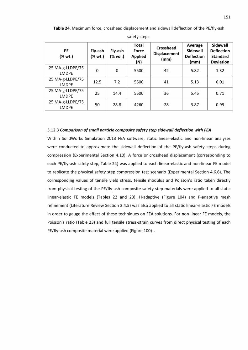
151

Table 24. Maximum force, crosshead displacement and sidewall deflection of the PE/fly-ash

safety steps.

PE (% wt.)

Fly-ash (% wt.)

Fly-ash (% vol.)

Total Force

Applied (N)

Crosshead Displacement

(mm)

Average Sidewall

Deflection (mm)

Sidewall Deflection Standard Deviation

25 MA-g-LLDPE/75 LMDPE

0 0 5500 42 5.82 1.32

25 MA-g-LLDPE/75 LMDPE

12.5 7.2 5500 41 5.13 0.01

25 MA-g-LLDPE/75 LMDPE

25 14.4 5500 36 5.45 0.71

25 MA-g-LLDPE/75 LMDPE

50 28.8 4260 28 3.87 0.99

5.12.3 Comparison of small particle composite safety step sidewall deflection with FEA

Within SolidWorks Simulation 2013 FEA software, static linear-elastic and non-linear analyses

were conducted to approximate the sidewall deflection of the PE/fly-ash safety steps during

compression (Experimental Section 4.10). A force or crosshead displacement (corresponding to

each PE/fly-ash safety step, Table 24) was applied to each linear-elastic and non-linear FE model

to replicate the physical safety step compression test scenario (Experimental Section 4.6.6). The

corresponding values of tensile yield stress, tensile modulus and Poisson’s ratio taken directly

from physical testing of the PE/fly-ash composite safety step materials were applied to all static

linear-elastic FE models (Tables 22 and 23). H-adaptive (Figure 104) and P-adaptive mesh

refinement (Literature Review Section 3.4.5) was also applied to all static linear-elastic FE models

in order to gauge the effect of these techniques on FEA solutions. For non-linear FE models, the

Poisson’s ratio (Table 23) and full tensile stress-strain curves from direct physical testing of each

PE/fly-ash composite material were applied (Figure 100) .

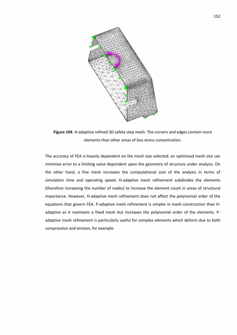
152

Figure 104. H-adaptive refined 3D safety step mesh. The corners and edges contain more

elements than other areas of less stress concentration.

The accuracy of FEA is heavily dependent on the mesh size selected; an optimised mesh size can

minimise error to a limiting value dependent upon the geometry of structure under analysis. On

the other hand, a fine mesh increases the computational cost of the analysis in terms of

simulation time and operating speed. H-adaptive mesh refinement subdivides the elements

(therefore increasing the number of nodes) to increase the element count in areas of structural

importance. However, H-adaptive mesh refinement does not affect the polynomial order of the

equations that govern FEA. P-adaptive mesh refinement is simpler in mesh construction than H-

adaptive as it maintains a fixed mesh but increases the polynomial order of the elements. P-

adaptive mesh refinement is particularly useful for complex elements which deform due to both

compression and tension, for example.

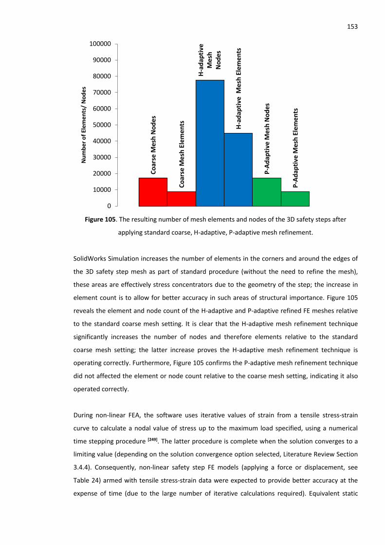
153

Figure 105. The resulting number of mesh elements and nodes of the 3D safety steps after

applying standard coarse, H-adaptive, P-adaptive mesh refinement.

SolidWorks Simulation increases the number of elements in the corners and around the edges of

the 3D safety step mesh as part of standard procedure (without the need to refine the mesh),

these areas are effectively stress concentrators due to the geometry of the step; the increase in

element count is to allow for better accuracy in such areas of structural importance. Figure 105

reveals the element and node count of the H-adaptive and P-adaptive refined FE meshes relative

to the standard coarse mesh setting. It is clear that the H-adaptive mesh refinement technique

significantly increases the number of nodes and therefore elements relative to the standard

coarse mesh setting; the latter increase proves the H-adaptive mesh refinement technique is

operating correctly. Furthermore, Figure 105 confirms the P-adaptive mesh refinement technique

did not affected the element or node count relative to the coarse mesh setting, indicating it also

operated correctly.

During non-linear FEA, the software uses iterative values of strain from a tensile stress-strain

curve to calculate a nodal value of stress up to the maximum load specified, using a numerical

time stepping procedure [249]. The latter procedure is complete when the solution converges to a

limiting value (depending on the solution convergence option selected, Literature Review Section

3.4.4). Consequently, non-linear safety step FE models (applying a force or displacement, see

Table 24) armed with tensile stress-strain data were expected to provide better accuracy at the

expense of time (due to the large number of iterative calculations required). Equivalent static

Co

arse

Mes

h N

od

es

Co

arse

Mes

h E

lem

en

ts

H-a

dap

tive

M

esh

N

od

es

H-a

dap

tive

Mes

h E

lem

en

ts

P-A

dap

tive

Mes

h N

od

es

P-A

dap

tive

Mes

h E

lem

en

ts

0

10000

20000

30000

40000

50000

60000

70000

80000

90000

100000

Nu

mb

er

of

Ele

me

nts

/ N

od

es

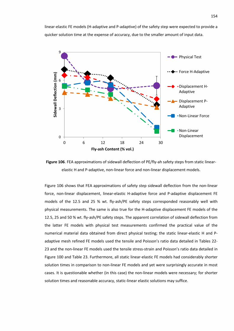
154 linear-elastic FE models (H-adaptive and P-adaptive) of the safety step were expected to provide a

quicker solution time at the expense of accuracy, due to the smaller amount of input data.

Figure 106. FEA approximations of sidewall deflection of PE/fly-ah safety steps from static linear-

elastic H and P-adaptive, non-linear force and non-linear displacement models.

Figure 106 shows that FEA approximations of safety step sidewall deflection from the non-linear

force, non-linear displacement, linear-elastic H-adaptive force and P-adaptive displacement FE

models of the 12.5 and 25 % wt. fly-ash/PE safety steps corresponded reasonably well with

physical measurements. The same is also true for the H-adaptive displacement FE models of the

12.5, 25 and 50 % wt. fly-ash/PE safety steps. The apparent correlation of sidewall deflection from

the latter FE models with physical test measurements confirmed the practical value of the

numerical material data obtained from direct physical testing; the static linear-elastic H and P-

adaptive mesh refined FE models used the tensile and Poisson’s ratio data detailed in Tables 22-

23 and the non-linear FE models used the tensile stress-strain and Poisson’s ratio data detailed in

Figure 100 and Table 23. Furthermore, all static linear-elastic FE models had considerably shorter

solution times in comparison to non-linear FE models and yet were surprisingly accurate in most

cases. It is questionable whether (in this case) the non-linear models were necessary; for shorter

solution times and reasonable accuracy, static-linear elastic solutions may suffice.

0

3

6

9

0 6 12 18 24 30

Sid

ewal

l De

flec

tio

n (

mm

)

Fly-ash Content (% vol.)

Physical Test

Force H-Adaptive

Displacement H-Adaptive

Displacement P-Adaptive

Non-Linear Force

Non-LinearDisplacement

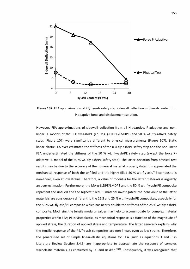
155

Figure 107. FEA approximation of PE/fly-ash safety step sidewall deflection vs. fly-ash content for

P-adaptive force and displacement solution.

However, FEA approximations of sidewall deflection from all H-adaptive, P-adaptive and non-

linear FE models of the 0 % fly-ash/PE (i.e. MA-g-LLDPE/LMDPE) and 50 % wt. fly-ash/PE safety

steps (Figure 107) were significantly different to physical measurements (Figure 107). Static

linear-elastic FEA over-estimated the stiffness of the 0 % fly-ash/PE safety step and the non-linear

FEA under-estimated the stiffness of the 50 % wt. fly-ash/PE safety step (except the force P-

adaptive FE model of the 50 % wt. fly-ash/PE safety step). The latter deviation from physical test

results may be due to the accuracy of the numerical material property data; it is appreciated the

mechanical response of both the unfilled and the highly filled 50 % wt. fly-ash/PE composite is

non-linear, even at low strains. Therefore, a value of modulus for the latter materials is arguably

an over-estimation. Furthermore, the MA-g-LLDPE/LMDPE and the 50 % wt. fly-ash/PE composite

represent the unfilled and the highest filled PE material investigated; the behaviour of the latter

materials are considerably different to the 12.5 and 25 % wt. fly-ash/PE composites, especially for

the 50 % wt. fly-ash/PE composite which has nearly double the stiffness of the 25 % wt. fly-ash/PE

composite. Modifying the tensile modulus values may help to accommodate for complex material

properties within FEA; PE is viscoelastic, its mechanical response is a function of the magnitude of

applied stress, the duration of applied stress and temperature. The latter generally explains why

the tensile response of the PE/fly-ash composites are non-linear, even at low strains. Therefore,

the generalised set of simple linear-elastic equations for FEA (such as equations 3 and 5 in

Literature Review Section 3.4.3) are inappropriate to approximate the response of complex

viscoelastic materials, as confirmed by Lai and Bakker [250]. Consequently, it was recognised that

4

7

10

13

16

19

22

0 6 12 18 24 30

Sid

ewal

l De

flec

tio

n (

mm

)

Fly-ash Content (% vol.)

Force P-Adaptive

Physical Test

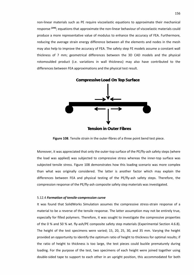
156 non-linear materials such as PE require viscoelastic equations to approximate their mechanical

response [249]; equations that approximate the non-linear behaviour of viscoelastic materials could

produce a more representative value of modulus to enhance the accuracy of FEA. Furthermore,

reducing the average strain energy difference between all the elements and nodes in the mesh

may also help to improve the accuracy of FEA. The safety step FE models assume a constant wall

thickness of 7 mm; geometrical differences between the 3D CAD models and the physical

rotomoulded product (i.e. variations in wall thickness) may also have contributed to the

differences between FEA approximations and the physical test result.

Figure 108. Tensile strain in the outer-fibres of a three point bend test piece.

Moreover, it was appreciated that only the outer-top surface of the PE/fly-ash safety steps (where

the load was applied) was subjected to compressive stress whereas the inner-top surface was

subjected tensile stress. Figure 108 demonstrates how this loading scenario was more complex

than what was originally considered. The latter is another factor which may explain the

differences between FEA and physical testing of the PE/fly-ash safety steps. Therefore, the

compression response of the PE/fly-ash composite safety step materials was investigated.

5.12.4 Formation of tensile-compression curve

It was found that SolidWorks Simulation assumes the compressive stress-strain response of a

material to be a reverse of the tensile response. The latter assumption may not be entirely true,

especially for filled polymers. Therefore, it was sought to investigate the compressive properties

of the 0 % and 50 % wt. fly-ash/PE composite safety step materials (Experimental Section 4.6.8).

The height of the test specimens were varied; 15, 20, 25, 30, and 35 mm. Varying the height

provided an opportunity to identify the optimum ratio of height to thickness for optimal results; if

the ratio of height to thickness is too large, the test pieces could buckle prematurely during

loading. For the purpose of the test, two specimens of each height were joined together using

double-sided tape to support to each other in an upright position, this accommodated for both

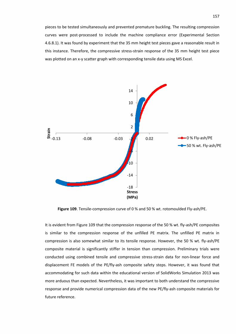
157 pieces to be tested simultaneously and prevented premature buckling. The resulting compression

curves were post-processed to include the machine compliance error (Experimental Section

4.6.8.1). It was found by experiment that the 35 mm height test pieces gave a reasonable result in

this instance. Therefore, the compressive stress-strain response of the 35 mm height test piece

was plotted on an x-y scatter graph with corresponding tensile data using MS Excel.

Figure 109. Tensile-compression curve of 0 % and 50 % wt. rotomoulded Fly-ash/PE.

It is evident from Figure 109 that the compression response of the 50 % wt. fly-ash/PE composites

is similar to the compression response of the unfilled PE matrix. The unfilled PE matrix in

compression is also somewhat similar to its tensile response. However, the 50 % wt. fly-ash/PE

composite material is significantly stiffer in tension than compression. Preliminary trials were

conducted using combined tensile and compressive stress-strain data for non-linear force and

displacement FE models of the PE/fly-ash composite safety steps. However, it was found that

accommodating for such data within the educational version of SolidWorks Simulation 2013 was

more arduous than expected. Nevertheless, it was important to both understand the compressive

response and provide numerical compression data of the new PE/fly-ash composite materials for

future reference.

-18

-14

-10

-6

-2

2

6

10

14

-0.13 -0.08 -0.03 0.02Stra

in

Stress(MPa)

0 % Fly-ash/PE

50 % wt. Fly-ash/PE

158 5.12.5 Key findings from the finite element analysis of PE/fly-ash safety steps

Investigating the FEM for the structural analysis of rotomoulded products made using a new

particulate-filled PE composite is particularly novel in the field of rotomoulding. Furthermore,

investigating the Poisson’s ratio and compressive properties of particulate-filled polymer

composites forms another novel aspect of this research. For the purpose of clarity, the key

findings of this investigation are summarised in the following bullet points:

The tensile yield stress, modulus and Poisson’s ratio are required for static linear-elastic

FE models. For non-linear FE models, the Poisson’s ratio and full tensile stress-strain

curves from direct physical testing of each PE/fly-ash composite material are required.

Calculating a consistent value of Poisson’s ratio was not possible at low to medium levels

of strain. However, significantly more consistent values of Poisson’s ratio were calculated

at higher levels of strain (close to or at the yield point).

The addition of fly-ash to MA-g-LLDPE had a relatively small effect on the Poisson’s ratio.

The 25 % wt. and 50 % wt. (14.4 and 28.8 % vol.) fly-ash/PE safety steps underwent

considerably less sidewall deflection relative to the unfilled and 12.5 % wt. (7.2 % vol.) fly-

ash/PE safety steps. However, the 50 % wt. fly-ash/PE steps fractured at 4.26 kN load.

The H-adaptive mesh refinement technique significantly increased the number of nodes

and therefore elements relative to the standard coarse mesh setting; the latter increase

proves the H-adaptive mesh refinement technique is operating correctly.

The P-adaptive mesh refinement technique did not affected the element or node count

relative to the coarse mesh setting, indicating it also operated correctly.

FEA approximations of safety step sidewall deflection from the non-linear force, non-

linear displacement, linear-elastic H-adaptive force and P-adaptive displacement FE

models of the 12.5 and 25 % wt. fly-ash/PE safety steps corresponded reasonably well

with physical measurements. The same is also true for the H-adaptive displacement FE

models of the 12.5, 25 and 50 % wt. fly-ash/PE safety steps.

All static linear-elastic FE models had considerably shorter solution times in comparison to

non-linear FE models and yet were surprisingly accurate in most cases. It is questionable

159

whether (in this case) the non-linear models were necessary; for shorter solution times

and reasonable accuracy, static-linear elastic solutions may suffice.

Static linear-elastic FEA over-estimated the stiffness of the 0 % fly-ash/PE safety step and

the non-linear FEA under-estimated the stiffness of the 50 % wt. fly-ash/PE safety step

(except the force P-adaptive FE model of the 50 % wt. fly-ash/PE safety step).

The compression response of the 50 % wt. fly-ash/PE composites is similar to the

compression response of the unfilled PE matrix. Moreover, the unfilled PE matrix in

compression is also somewhat similar to its tensile response. However, the 50 % wt. fly-

ash/PE composite material is significantly stiffer in tension than compression.

5.12.6 Key considerations for the finite element analysis of rotomoulded parts

The combined effect of various complex factors on FEA such as FE model assumptions, the non-

linear behaviour of PE and the variation in wall thickness of rotomoulded parts exemplified the

importance of properly understanding FEA software; basic to intermediate users can create 3D

structures, apply forces, constraints and material data with relatively little effort. Therefore, the

following considerations should be made when using FEA software:

Understand the boundary conditions (loads, constraints and material data). Ensure a

simplified, representative loading scenario of the FE model for quicker solutions.

Ensure the dimensions of the structure under analysis are accurately defined.

Validate the FEA softwares calculations by hand (e.g. simple beam bending theory)

Use FEA to identify areas of the structure beyond the yield stress of the material or

maximum deflection required.

Determine experimental error.

160

6. Conclusions

The investigations detailed in this thesis have resulted in several interesting conclusions regarding

both the development of PE/filler composite materials for RM and the consequent application of

FEA in order to numerically approximate the mechanical response of rotomoulded parts using

such materials. These are summarised in the following paragraphs:

6.1 Mechanical Properties

In terms of the mechanical properties and processability of the proposed PE/filler composites, the

original aims this study (Section 1.1) were to:

Evaluate a selection of particulate fillers as reinforcement to RM grade PE in order to

double its tensile modulus.

Optimise the chosen composite system for performance and processability.

The aim of doubling the modulus of rotomoulding grade PE using a particulate filler was achieved

at 28.8 % vol. fly-ash for composites based on a blend of 25 % wt. MA-g-LLDPE with 75 % wt.

LMDPE (Figure 90, Results and Discussion Section 5.9.2); these observations verify the claimed

coupling activity of the MA-g-LLDPE with the finer fly-ash particles. Furthermore, at 28.8 % vol. fly-

ash loading, the tensile stress at yield (Figure 91) remains effectively the same as the unfilled

matrix (when taking the data variation into account). However, the impact strength of the

rotomoulded PE/fly-ash composites (Figure 92) decreased with every filler loading investigated;

this was especially true for the 28.8 % vol. PE/fly-ash composites where the impact strength fell

by approximately 88 %. The latter is unacceptable for rotomoulded applications such as

underground water tanks or kayaks where the toughness and ductility of unfilled PE is essential.

Therefore, future investigations to enhance the toughness of the PE/fly-ash composites are

detailed in Section 7. Physical observations also confirmed that the PE/fly-ash composites were

increasingly more brittle with the increase in fly-ash loading, relative to the ductile unfilled matrix.

Moreover, the MFR of the PE/fly-ash composites decreased with the addition of fly-ash. In terms

of modulus enhancement (Figure 90) the optimum fly-ash loading of 28.8 % vol. corresponds to a

42 % loss in MFR relative to the unfilled matrix (Figure 88). Such a loss in MFR placed a question

mark over the feasibility of the PE/fly-ash composites for rotomoulding applications. However,

experimental data suggests an optimal balance between the tensile modulus (Figure 90), yield

161 stress (Figure 91) and MFR (Figure 88) of rotomoulded PE may be possible at fly-ash loadings

between 14-28 % vol.; this should not be problematic to rotomould in powder form.

6.2 Filler-Matrix Blending Technique

Dry blending of coarse particle fillers (i.e. sand, garnet and cenospheres) with powdered LMDPE/

MA-g-LLDPE blends followed by compression moulding generally gave composites with poor

mechanical properties relative to equivalent composites where the filler particles were melt

blended in to the same matrix using a two roll mill. Twin screw extrusion melt blending of

composites based on the finer fillers (i.e. fly-ash) was also successful and produced compression

mouldings with excellent mechanical properties. However, the improvements in tensile modulus

and yield stress were accompanied by reduced impact toughness at high fly-ash loadings (50 %

wt.) where the stiffness enhancement was more prominent. Furthermore, the addition of fly-ash

impacts the melt flow behaviour of PE in a largely negative way.

6.3 Polyethylene, Filler and Coupling Agent

Compression moulded, melt blended MA-g-LLDPE/LMDPE blends with the addition of finer filler

(i.e. fly-ash) had excellent mechanical properties. Remarkably, the TSE melt blended compression

moulded highly-filled fly-ash/LMDPE (70 % wt.) composites displayed improvements in strength

which showed signs of stabilising at 20-25 % MA-g-LLDPE. For equivalent HDPE composites,

maximum stress was observed at 10 % wt. MA-g-LLDPE; the latter is probably due to poor

compatibility between HDPE and MA-g-LLDPE due to the relatively high level of branching in MA-

g-LLDPE. HDPE was initially selected for reinforcement with fly-ash particles due to its higher

stiffness than LMDPE. However, better compatibility was observed between MA-g-LLDPE/LMDPE

with the addition of fly-ash; these observations verify the claimed coupling activity of the MA-g-

LLDPE with the finer fly-ash particles. Consequently, in the context of melt flow properties and

cost, it was decided that the MA-g-LLDPE/LMDPE-fly-ash blends were more suitable for

rotomoulding relative to the added expense and reduced melt flow properties of equivalent MA-

g-LLDPE/HDPE composites. Therefore, MA-g-LLDPE/LMDPE-fly-ash blends were selected for

rotational moulding. High temperature flexural tests revealed the addition of fly-ash to MA-g-

LLDPE/LMDPE system improved the heat distortion behaviour of the resulting injection moulded

composites relative to the unfilled matrix.

162 6.4 Fillers - Effect of Bimodal Particle Size Distribution

Maximum packing fraction determinations (using a modified oil absorption type test) confirmed

that combinations of fly-ash and cenospheres could boost filler volume fraction in the composites.

However, the mechanical response of these mixed filler composites was poor (in most cases

poorer than with fly-ash alone). Bearing in mind the fact that the cenospheres form only a small

fraction (ca. 2 %) of fuel ash from power stations and their relatively high cost, it was concluded

that a filler system based on fly-ash/cenosphere combinations is not a viable option. During these

preliminary melt blending trials, the small particle size fillers (i.e. fly-ash) performed best due to

the fact that they do not act as large defects in the matrix and they provide sufficient interfacial

area for the effective deployment of the MA-g-LLDPE coupling agent.

6.5 Small Particle Composites – Properties in the Context of Rotational Moulding

The objective of doubling the tensile modulus of MA-g-LLDPE/LMDPE based blends was achieved

at fly ash volume fractions between 20-30 % for compression moulded samples; the latter fly-ash

loading was not considered over problematic in the context of rotational moulding. It was found

that rotomoulded safety steps made using the TSE melt blended maleanised PE/fly-ash composite

materials offered stiffness comparable to that of higher density rotomoulding PE grades at the

highest fly-ash loading investigated (28.8 % vol.). However, pinholes on the surface of

rotomoulded PE increased with the addition of fly-ash; the addition fly-ash significantly decreases

the MFR of the composite melt which complicates processability. The latter confirmed the

challenge in using such highly filled PE composites for the zero-shear rotomoulding process.

However, the variation in wall thickness of rotomoulded PE safety steps decreased with the

addition of fly-ash; the loss in the MFR of the composite melt with the addition of fly-ash reduced

the amount of bulk flow of the melt during rotomoulding, thus preventing material from

gathering in the corners of the mould resulting in greater wall thickness uniformity.

The latter rotomoulded PE/fly-ash composite safety steps were compression tested and

measured for sidewall deflection. Computer simulation of the rotomoulded PE/fly-ash safety

steps sidewall deflection was conducted using FEA software. Poisson’s ratio values for the PE/fly-

ash composite safety step materials were required for FEA. Currently, there is little available

literature regarding the Poisson’s ratio of PE; for the vast majority of materials such as metals,

ceramics and some polymers (including PE), the Poisson’s ratio is assumed to be between 0.3-0.5

[243]. Measuring the Poisson’s ratio of PE is a challenge due to the non-linear behaviour of PE very

low strains; it was found that calculating a consistent value of Poisson’s ratio was not possible at

163 the low to medium levels of strain. However, significantly more consistent values of Poisson’s

ratio were calculated at higher levels of strain (close to and at the yield point). Therefore, the

resulting values of Poisson’s ratio were close to or at the yield point, rather than within the elastic

region (Experimental Section 4.6.4.1). However, it was observed the addition of fly-ash to MA-g-

LLDPE had a relatively small effect on the Poisson’s ratio. Recent published work associated with

this thesis concluded that reasonable values of Poisson’s ratio between 0.3-0.5 had a minimal

impact on FEA of the rotomoulded safety steps [248].

6.6 Finite Element Analysis of Rotomoulded Small Particle Composites

The numerical material parameters required for FEA of the new high stiffness PE/fly-ash

composite material was the tensile modulus, stress at yield, Poisson’s ratio and full tensile stress-

strain curves (for non-linear analyses). Measured values of sidewall deflection for the

rotomoulded PE/fly-ash safety steps coincided reasonably well with FEA approximations from the

static linear-elastic and non-linear FE models (depending on the mesh refinement type and

material data applied to the FE model), confirming the practical value of the numerical material

data. However, in some instances significant differences between FEA and the actual safety step

were probably due to the effect of various complex factors such as the non-linear behaviour of PE

and the variation in wall thickness of rotomoulded parts. These differences between the

assumptions of the FE model and the physical rotomoulded part contribute to the accuracy of

FEA, exemplifying the importance of verifying how FEA software calculates a solution. The

following considerations should be taken into account when using FEA software for rotomoulded

products:

Understand the analysis type.

Understand the boundary conditions (loads, constraints and material data). Ensure a

simplified, representative loading scenario of the FE model for quicker solutions.

Ensure the dimensions of the structure under analysis are accurately defined.

Validate the FEA software’s calculations by hand (e.g. simple beam bending theory)

Use FEA to identify areas beyond the yield stress of the material or maximum

deflection.

Determine experimental error.

164 6.7 Overall Recommendations

A substantial variety of sample preparation and experimental methods were implemented to

enhance the modulus of PE. Consequently, an optimum formulation for further investigation is

suggested in the following paragraphs.

1. The fly-ash particles can double the tensile modulus of PE at levels that are acceptable to

rotomould (ca. 30 % wt., even without the MA coupling agent). Furthermore, the small

size and spherical shape of the fly-ash particles give sufficient interfacial area for the

effective deployment of the MA-g-LLDPE coupling agent. Therefore, it is recommended to

use the fly-ash particles for further investigation.

2. The MA coupling agent grafted LLDPE blended with LMDPE is a versatile matrix in terms

of compatibility with the fly-ash particles; it is apparent that increasing the level MA-g-

LLDPE in LMDPE increases the modulus at lower levels. Furthermore, the tensile yield

stress of LMDPE/fly-ash composites increases with every level of MA-g-LLDPE (up to 25 %

wt.). Due to the strong interaction of the MA-g-LLDPE/LMDPE blends with the fly-ash

particles and the arguably more suitable MFR of the latter PE blends for rotomoulding

(relative to alternative PE grades such as HDPE), it is recommended to remain with this

particular blend of PE for further investigation.

3. The PE and fly-ash should be blended by TSE compounding prior to moulding, rather than

dry blending or two roll mill blending. The TSE compounded composites had the best

mechanical properties relative to two roll milled or dry blended equivalents; this is

because the matrix and filler particles are blended under electro-mechanically controlled

shear force and temperature, ensuring better dispersion of the filler particles in the

matrix, homogeneity and reproducibility. Furthermore, TSE compounding improves the

effectiveness of the MA-g-LLDPE coupling agent.

4. Tensile, flexural, Charpy impact and MFR tests are effective methods of gauging the

modulus, strength, impact toughness and melt flow properties of the PE/fly-ash

composites. However, it is suggested that zero-shear viscometry be conducted to gauge

the MFR of the PE/fly-ash composites under the zero-shear conditions encountered in

rotomoulding. Furthermore, one intended application of the PE/fly-ash composites is

underground water tanks. Therefore, creep tests on actual rotomoulded tanks are

essential at some point of the development phase.

165

5. The tensile modulus, stress at yield, Poisson’s ratio and full tensile stress strain curves are

required for FEA, (the latter is required for non-linear analyses). However, it should be

appreciated that the moduli of non-linear materials are an over-estimation when

calculated using a conventional method. Therefore, it is recommended that the moduli of

the PE/fly-ash composites are re-calculated to a more representative value for the

purpose of FEA; linear viscoelastic equations may be explored to accommodate for this.

Moreover, it is crucial to understand the principles of FEA properly in order to represent

the loading scenario accurately (e.g. the type of analysis selected and other application-

specific factors such as the variation in wall thickness of rotomoulded products).

With further development, especially in terms of MFR and impact toughness, it is envisaged that

the PE/fly-ash composite can provide the required modulus enhancement to PE whilst

maintaining suitable impact and melt flow properties for rotomoulding. Upon achieving the latter

objective, a numerical database of material properties can be compiled for comparative stress

analysis studies (using FEA) of virgin PE tanks versus the new high stiffness PE/fly-ash composite

tanks. Theoretically, the high modulus PE/fly-ash composite material can lower the wall thickness

of load-bearing rotomoulded components whilst maintaining an acceptable factor of safety. If the

latter is achieved, real tanks could be rotomoulded and physically tested for comparison with FEA

to validate the material data and prove the effectiveness of the PE/fly-ash composite at lowering

the wall thickness, due to its relatively high modulus.

166

7. Further Work

The PE/filler composites detailed in this thesis led to a number of different development

formulations. However, it is apparent that fly-ash particles provide the best mechanical

improvements to PE; the most viable composite system investigated thus far is that based on

LMDPE and fly ash with an MA-g-LLDPE coupling agent. With the latter system, the objective of

doubling the tensile modulus can be achieved at high fly ash volume fractions for rotomoulding

applications (28 % vol.). Therefore, future investigations would still remain with optimising the

PE/fly-ash blends for rotomoulding. However, the latter 28 % vol. fly-ash/PE composite had low

MFR and impact properties, consequently leading to poor part surface quality. Investigations have

suggested an optimal balance between the tensile modulus, strength and processability of

rotomoulded PE may be possible at fly-ash loadings between 14-28 % vol.; this should not be

problematic to rotomould in powder form. The following points summarise the future work

suggested as a result of this study:

Development of thermo-oxidative stabilisation strategies for the PE/fly-ash composites

with a view to maximising processability - examining novel and sustained release

stabilisation strategies for the MA-g-LLDPE/LMDPE blend with the addition of fly-ash is

necessary for optimising the composite materials suitability for RM. Large rotomoulded

parts such as underground water tanks or liquid storage silos take considerably long to

manufacture (typically 8 hours duration at above 200 oC for a 10,000 litre PE tank).

Therefore, it is crucial to investigate (and improve) the stability of the PE/fly-ash

composite in such harsh processing conditions.

Assess the zero shear melt flow rate of PE fly-ash composites - zero-shear viscometry is a

more precise method of analysing the melt flow properties of the PE/fly-ash composites

under conditions closer to those encountered in RM. The MFR of the rotomoulded MA-g-

LLDPE/LMDPE blend is significantly reduced at the optimum fly-ash loading of 28.8 % in

terms of modulus enhancement. Cryogenic grinding of the TSE compounded PE/fly-ash

composite pellets to powder form and the addition of small amounts of powdered PE

during rotomoulding may improve processability.

Improve the impact strength of the PE/fly-ash composites - the addition of fly-ash

particles to PE has a detrimental effect on the impact properties of the resulting

composites. The latter can potentially be improved by incorporating an elastomeric

167

component in the composite to instil toughness. Furthermore, wetting agents such as

Silanes can also be used to improve toughness via a reduction in the surface energy of the

filler particles to better distribute them within the matrix. However, it is understood that

increasing the toughness of the composite in this way will probably have a negative effect

on the modulus and strength of the composite. Moreover, a multi-layer composite

structure (sandwich laminate) could provide a good balance between the impact

properties and tensile modulus of the PE/fly-ash composites. The industrial sponsor has

extensive experience in utilising commercially established techniques for multi-layer

laminate materials.

Development of creep data for the purpose of FEA - numerical creep data from the

PE/fly-ash composites will be required to create FE models of real RM products such as

underground water tanks for creep analysis. A key mechanical parameter for design

engineers is creep data; development of the latter can provide tailor made materials

modelling tools for design engineers expected to model the new materials. Creep tests in

three point bend mode are often at elevated temperature (typically 50 °C) for typically

1000 hours duration. Therefore, careful advance planning is required. The industrial

sponsor constructed an in-house creep testing facility used to examine the creep

behaviour of the new PE/fly-ash composite materials. Initial tests have indicated the

material lifetime of the highly filled PE/fly-ash composite is considerably longer than

unfilled LMDPE i.e. for a given lifetime the stress withstood by the latter composite is

significantly greater than that of unfilled LMDPE.

FEA of industrial-scale rotomoulded PE/fly-ash load-bearing parts - thus far, FEA has

been applied to a relatively small (commercial-scale) rotomoulded safety step using

numerical materials data from physical testing of the PE/flash composite materials. The

rotomoulded safety step had a relatively simple loading scenario and was practical for

small-scale testing at MMU. However, it is appreciated that the effect of non-linear

material behaviour and the variations in wall thickness of much larger rotomoulded parts

(such as oil storage silos) presents a considerably more complex challenge for FEA,

possibly requiring more advanced physical testing and FE modelling methods; it is

envisaged that non-linear viscoelastic equations will be used to provide a more

representative value of modulus (with respect to time, stress and temperature) for FEA.

168

8. References

1. Crawford, R.J. Rotational Moulding of Plastics 2nd edition, John Wiley and Sons Inc., May

1996.

2. Krohn, J.V. Hughes, BJ. Mcfaddin, DC. Todd, WG. Higher Performance Polyethylene

Powder, Equistar Chemicals Ltd, Society of Plastics Engineers ANTEC Conference

Proceedings, page 1, May 2005.

3. Sowa, M.W. Rotational moulding of reinforced PE, SPE Journal, 26, pp 31-34. July 1970.

4. European Plastics News Magazine. Rotational process for GRP developed in Japan, page

42. January 1975.

5. Mohr, J.G. Rotational Moulding of Fibre Glass Reinforced Thermoplastics, SPI Handbook of

Technology and Engineering of Reinforced Plastics/Composites 2nd Edition, Chapter 6,

1981.

6. Plastics world Magazine. Rotomoulded RP – Exciting route to new markets, June 1970.

7. Ogasawara, Y. Tsuji, S. Yamamoto, R. A New Continuous Rotational Moulding Process for

RP Composition – CRM Process, Polym. Plast. Technol. Eng, 24 (1), pp. 1-10. 1985.

8. Miller, D.L. Fibre Glass Reinforced Plastic in Furniture, Society of Plastics Engineers ANTEC

(Annual Technical) Conference Proceedings, Section 16-C, pp. 1-4. 1975.

9. Kobe Steel Ltd. Method of Rotational Moulding Reinforcer-Incorporated Plastics, Japan,

United States Patent No. 3,981,955, September 1976.

10. Rotoplas Ltd. Method for the production of Reinforced Rotationally Moulded

Thermoplastic Articles, Jerusalem British Patent No. 1,381,863, January 1973.

11. Rotoplas Ltd. Method for Producing a Layer of Fibre – Reinforced Rotationally Moulded

Plastic Material, Jerusalem, European Patent No. 0,022,165, January 1981.

169 12. Wisley, B.W. PhD Thesis, Improving the Mechanical Properties of Rotomoulded Products,

Queens University Belfast, September 1994.

13. Murphy, M. MSc Thesis, An Investigation into the effect of Incorporating Glass and

Ceramic Microspheres in Rotationally Moulded Articles, Queens University Belfast,

September 1997.

14. Arnaud, R. Crawford R.J. The effects of fillers on the properties of rotationally moulded

Polyethylene, Polymer Processing Research Centre, Queens University Belfast, Society of

Plastics Engineers ANTEC Conference Proceedings, June 2002.

15. Hanna, P.R.W. McNally, T. Harkin-Jones, E. McMillan, P. Mechanical Properties of

Rotationally Moulded Nano-Composites, Queens University Belfast, Society of Plastics

Engineers ANTEC Conference Proceedings, May 2004.

16. Kanokboriboon, A. Sae-Chieng, W. An Investigation on the Effects of Fine-Particulate Filler

on the Properties of a Rotomoulding-Grade Polyethylene, King Mongkut Institute of

Technology North Bangkok and SCG Chemicals Co. Ltd. Thailand, Society of Plastics

Engineers ANTEC Conference Proceedings, January 2007.

17. Chang, W. C. Harkin-Jones, E. Kearns, M. McCourt, M. Glass Fibre-Reinforced PE

Composites in Rotational Moulding, Polymer Processing Research Centre, Queen’s

University Belfast, Society of Plastics Engineers ANTEC Conference Proceedings, May

2011.

18. Ward, J. Panigrahi, S. Tabil, L.G. Crerar, W.J. Powell, T. Rotational Molding of Flax Fiber

Reinforced Thermoplastic, Department of Agricultural and Bioresource Engineering,

University of Saskatchewan Canada. September 2002.

19. Butora, P. Náplava, A. Ridzon , M. Bílik, J. Tittel, V. Particle Filled Polyethylene Composites

Used in the Technology of Rotational Moulding, Institute of Materials Science, Faculty of

Materials Science and Technology, Slovak University of Technology, Slovakia. March 2012.

20. Lopez-Banuelos, R.H. Moscoso, F.J. Ortega-Gudino, P. Mendizabal, E. Rodrigue D.

Gonzalez-Nunez R. Rotational Molding of Polyethylene Composites Based on Agave

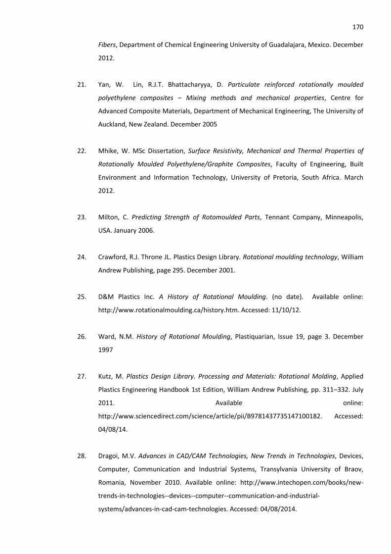
170

Fibers, Department of Chemical Engineering University of Guadalajara, Mexico. December

2012.

21. Yan, W. Lin, R.J.T. Bhattacharyya, D. Particulate reinforced rotationally moulded

polyethylene composites – Mixing methods and mechanical properties, Centre for

Advanced Composite Materials, Department of Mechanical Engineering, The University of

Auckland, New Zealand. December 2005

22. Mhike, W. MSc Dissertation, Surface Resistivity, Mechanical and Thermal Properties of

Rotationally Moulded Polyethylene/Graphite Composites, Faculty of Engineering, Built

Environment and Information Technology, University of Pretoria, South Africa. March

2012.

23. Milton, C. Predicting Strength of Rotomoulded Parts, Tennant Company, Minneapolis,

USA. January 2006.

24. Crawford, R.J. Throne JL. Plastics Design Library. Rotational moulding technology, William

Andrew Publishing, page 295. December 2001.

25. D&M Plastics Inc. A History of Rotational Moulding. (no date). Available online:

http://www.rotationalmoulding.ca/history.htm. Accessed: 11/10/12.

26. Ward, N.M. History of Rotational Moulding, Plastiquarian, Issue 19, page 3. December

1997

27. Kutz, M. Plastics Design Library. Processing and Materials: Rotational Molding, Applied

Plastics Engineering Handbook 1st Edition, William Andrew Publishing, pp. 311–332. July

2011. Available online:

http://www.sciencedirect.com/science/article/pii/B9781437735147100182. Accessed:

04/08/14.

28. Dragoi, M.V. Advances in CAD/CAM Technologies, New Trends in Technologies, Devices,

Computer, Communication and Industrial Systems, Transylvania University of Braov,

Romania, November 2010. Available online: http://www.intechopen.com/books/new-

trends-in-technologies--devices--computer--communication-and-industrial-

systems/advances-in-cad-cam-technologies. Accessed: 04/08/2014.

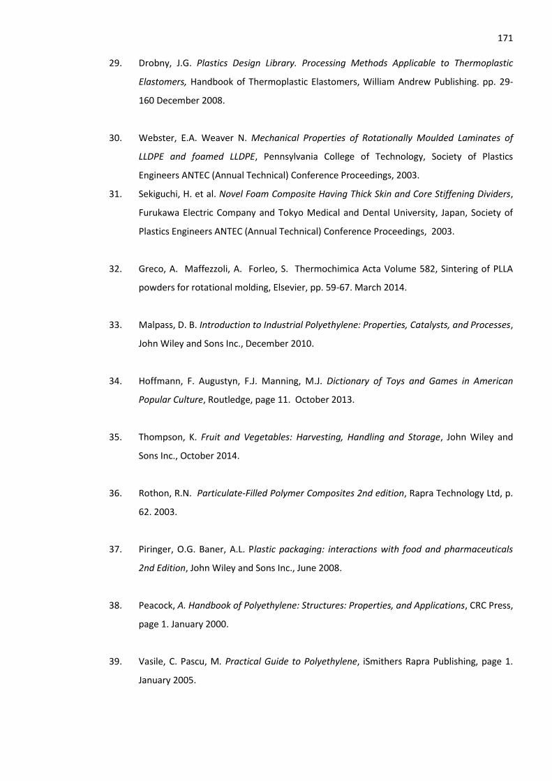
171 29. Drobny, J.G. Plastics Design Library. Processing Methods Applicable to Thermoplastic

Elastomers, Handbook of Thermoplastic Elastomers, William Andrew Publishing. pp. 29-

160 December 2008.

30. Webster, E.A. Weaver N. Mechanical Properties of Rotationally Moulded Laminates of

LLDPE and foamed LLDPE, Pennsylvania College of Technology, Society of Plastics

Engineers ANTEC (Annual Technical) Conference Proceedings, 2003.

31. Sekiguchi, H. et al. Novel Foam Composite Having Thick Skin and Core Stiffening Dividers,

Furukawa Electric Company and Tokyo Medical and Dental University, Japan, Society of

Plastics Engineers ANTEC (Annual Technical) Conference Proceedings, 2003.

32. Greco, A. Maffezzoli, A. Forleo, S. Thermochimica Acta Volume 582, Sintering of PLLA

powders for rotational molding, Elsevier, pp. 59-67. March 2014.

33. Malpass, D. B. Introduction to Industrial Polyethylene: Properties, Catalysts, and Processes,

John Wiley and Sons Inc., December 2010.

34. Hoffmann, F. Augustyn, F.J. Manning, M.J. Dictionary of Toys and Games in American

Popular Culture, Routledge, page 11. October 2013.

35. Thompson, K. Fruit and Vegetables: Harvesting, Handling and Storage, John Wiley and

Sons Inc., October 2014.

36. Rothon, R.N. Particulate-Filled Polymer Composites 2nd edition, Rapra Technology Ltd, p.

62. 2003.

37. Piringer, O.G. Baner, A.L. Plastic packaging: interactions with food and pharmaceuticals

2nd Edition, John Wiley and Sons Inc., June 2008.

38. Peacock, A. Handbook of Polyethylene: Structures: Properties, and Applications, CRC Press,

page 1. January 2000.

39. Vasile, C. Pascu, M. Practical Guide to Polyethylene, iSmithers Rapra Publishing, page 1.

January 2005.

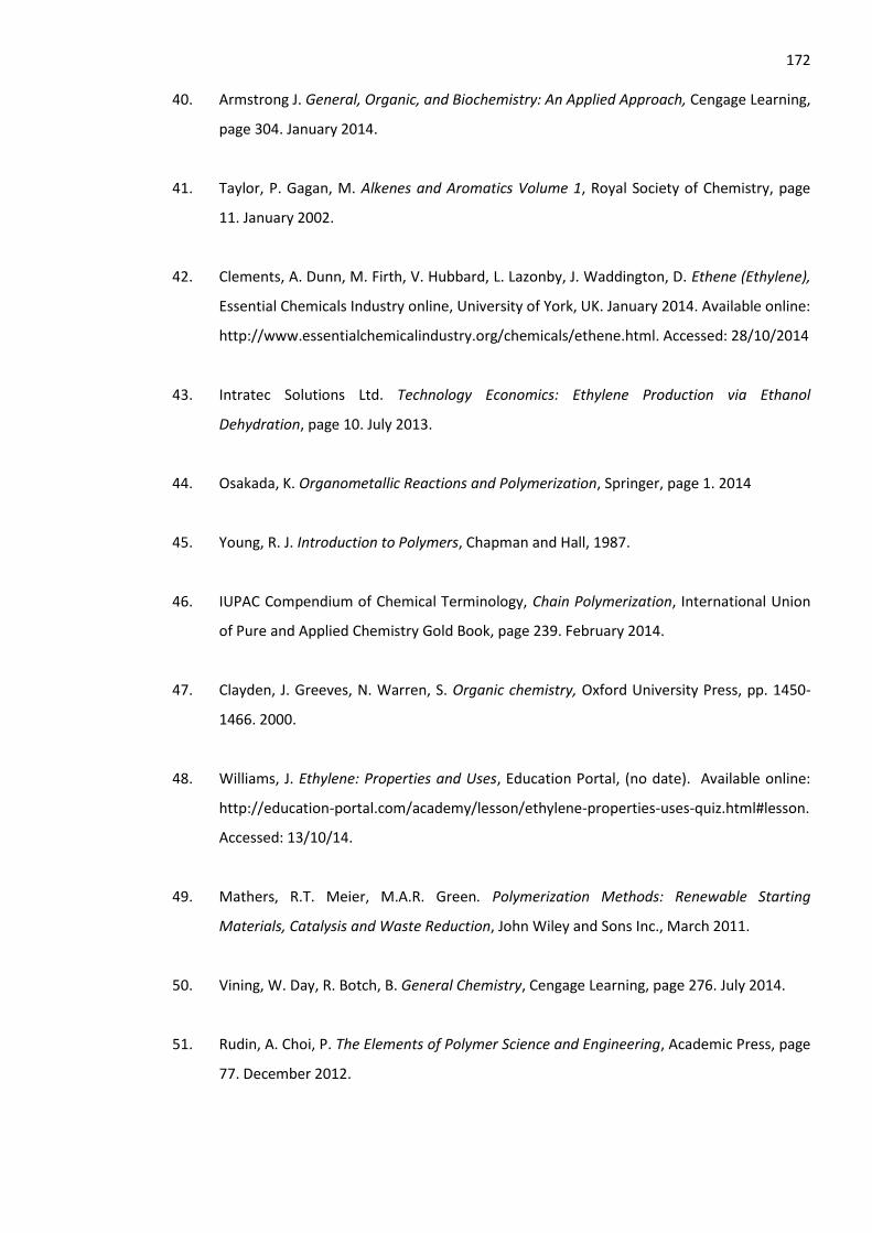
172 40. Armstrong J. General, Organic, and Biochemistry: An Applied Approach, Cengage Learning,

page 304. January 2014.

41. Taylor, P. Gagan, M. Alkenes and Aromatics Volume 1, Royal Society of Chemistry, page

11. January 2002.

42. Clements, A. Dunn, M. Firth, V. Hubbard, L. Lazonby, J. Waddington, D. Ethene (Ethylene),

Essential Chemicals Industry online, University of York, UK. January 2014. Available online:

http://www.essentialchemicalindustry.org/chemicals/ethene.html. Accessed: 28/10/2014

43. Intratec Solutions Ltd. Technology Economics: Ethylene Production via Ethanol

Dehydration, page 10. July 2013.

44. Osakada, K. Organometallic Reactions and Polymerization, Springer, page 1. 2014

45. Young, R. J. Introduction to Polymers, Chapman and Hall, 1987.

46. IUPAC Compendium of Chemical Terminology, Chain Polymerization, International Union

of Pure and Applied Chemistry Gold Book, page 239. February 2014.

47. Clayden, J. Greeves, N. Warren, S. Organic chemistry, Oxford University Press, pp. 1450-

1466. 2000.

48. Williams, J. Ethylene: Properties and Uses, Education Portal, (no date). Available online:

http://education-portal.com/academy/lesson/ethylene-properties-uses-quiz.html#lesson.

Accessed: 13/10/14.

49. Mathers, R.T. Meier, M.A.R. Green. Polymerization Methods: Renewable Starting

Materials, Catalysis and Waste Reduction, John Wiley and Sons Inc., March 2011.

50. Vining, W. Day, R. Botch, B. General Chemistry, Cengage Learning, page 276. July 2014.

51. Rudin, A. Choi, P. The Elements of Polymer Science and Engineering, Academic Press, page

77. December 2012.

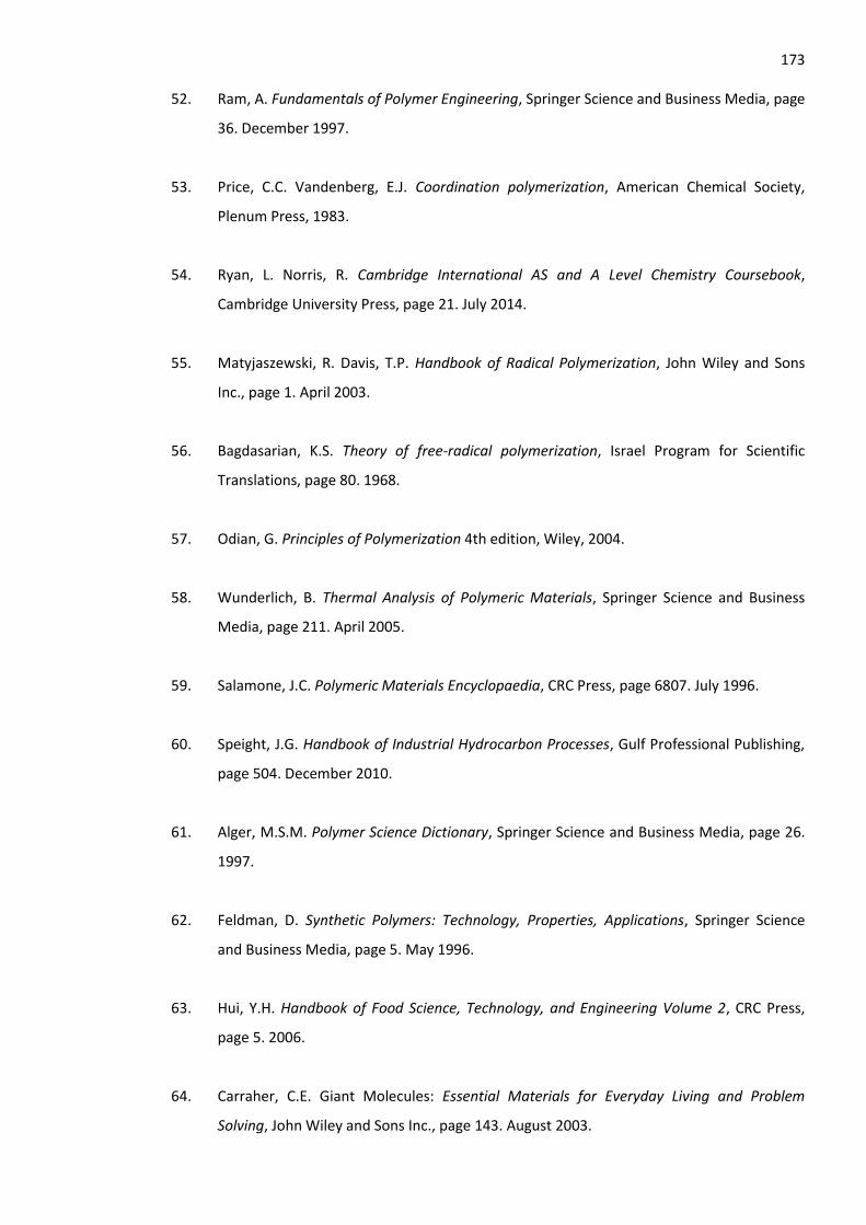
173 52. Ram, A. Fundamentals of Polymer Engineering, Springer Science and Business Media, page

36. December 1997.

53. Price, C.C. Vandenberg, E.J. Coordination polymerization, American Chemical Society,

Plenum Press, 1983.

54. Ryan, L. Norris, R. Cambridge International AS and A Level Chemistry Coursebook,

Cambridge University Press, page 21. July 2014.

55. Matyjaszewski, R. Davis, T.P. Handbook of Radical Polymerization, John Wiley and Sons

Inc., page 1. April 2003.

56. Bagdasarian, K.S. Theory of free-radical polymerization, Israel Program for Scientific

Translations, page 80. 1968.

57. Odian, G. Principles of Polymerization 4th edition, Wiley, 2004.

58. Wunderlich, B. Thermal Analysis of Polymeric Materials, Springer Science and Business

Media, page 211. April 2005.

59. Salamone, J.C. Polymeric Materials Encyclopaedia, CRC Press, page 6807. July 1996.

60. Speight, J.G. Handbook of Industrial Hydrocarbon Processes, Gulf Professional Publishing,

page 504. December 2010.

61. Alger, M.S.M. Polymer Science Dictionary, Springer Science and Business Media, page 26.

1997.

62. Feldman, D. Synthetic Polymers: Technology, Properties, Applications, Springer Science

and Business Media, page 5. May 1996.

63. Hui, Y.H. Handbook of Food Science, Technology, and Engineering Volume 2, CRC Press,

page 5. 2006.

64. Carraher, C.E. Giant Molecules: Essential Materials for Everyday Living and Problem

Solving, John Wiley and Sons Inc., page 143. August 2003.

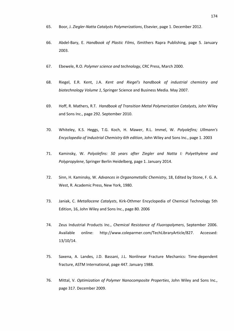
174 65. Boor, J. Ziegler-Natta Catalysts Polymerizations, Elsevier, page 1. December 2012.

66. Abdel-Bary, E. Handbook of Plastic Films, iSmithers Rapra Publishing, page 5. January

2003.

67. Ebewele, R.O. Polymer science and technology, CRC Press, March 2000.

68. Riegel, E.R. Kent, J.A. Kent and Riegel's handbook of industrial chemistry and

biotechnology Volume 1, Springer Science and Business Media. May 2007.

69. Hoff, R. Mathers, R.T. Handbook of Transition Metal Polymerization Catalysts, John Wiley

and Sons Inc., page 292. September 2010.

70. Whiteley, K.S. Heggs, T.G. Koch, H. Mawer, R.L. Immel, W. Polyolefins; Ullmann's

Encyclopedia of Industrial Chemistry 6th edition, John Wiley and Sons Inc., page 1. 2003

71. Kaminsky, W. Polyolefins: 50 years after Ziegler and Natta I: Polyethylene and

Polypropylene, Springer Berlin Heidelberg, page 1. January 2014.

72. Sinn, H. Kaminsky, W. Advances in Organometallic Chemistry, 18, Edited by Stone, F. G. A.

West, R. Academic Press, New York, 1980.

73. Janiak, C. Metallocene Catalysts, Kirk-Othmer Encyclopedia of Chemical Technology 5th

Edition, 16, John Wiley and Sons Inc., page 80. 2006

74. Zeus Industrial Products Inc., Chemical Resistance of Fluoropolymers, September 2006.

Available online: http://www.coleparmer.com/TechLibraryArticle/827. Accessed:

13/10/14.

75. Saxena, A. Landes, J.D. Bassani, J.L. Nonlinear Fracture Mechanics: Time-dependent

fracture, ASTM International, page 447. January 1988.

76. Mittal, V. Optimization of Polymer Nanocomposite Properties, John Wiley and Sons Inc.,

page 317. December 2009.

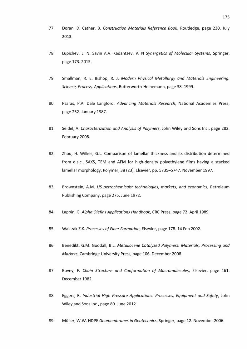
175 77. Doran, D. Cather, B. Construction Materials Reference Book, Routledge, page 230. July

2013.

78. Lupichev, L. N. Savin A.V. Kadantsev, V. N Synergetics of Molecular Systems, Springer,

page 173. 2015.

79. Smallman, R. E. Bishop, R. J. Modern Physical Metallurgy and Materials Engineering:

Science, Process, Applications, Butterworth-Heinemann, page 38. 1999.

80. Psaras, P.A. Dale Langford. Advancing Materials Research, National Academies Press,

page 252. January 1987.

81. Seidel, A. Characterization and Analysis of Polymers, John Wiley and Sons Inc., page 282.

February 2008.

82. Zhou, H. Wilkes, G.L. Comparison of lamellar thickness and its distribution determined

from d.s.c., SAXS, TEM and AFM for high-density polyethylene films having a stacked

lamellar morphology, Polymer, 38 (23), Elsevier, pp. 5735–5747. November 1997.

83. Brownstein, A.M. US petrochemicals: technologies, markets, and economics, Petroleum

Publishing Company, page 275. June 1972.

84. Lappin, G. Alpha Olefins Applications Handbook, CRC Press, page 72. April 1989.

85. Walczak Z.K. Processes of Fiber Formation, Elsevier, page 178. 14 Feb 2002.

86. Benedikt, G.M. Goodall, B.L. Metallocene Catalyzed Polymers: Materials, Processing and

Markets, Cambridge University Press, page 106. December 2008.

87. Bovey, F. Chain Structure and Conformation of Macromolecules, Elsevier, page 161.

December 1982.

88. Eggers, R. Industrial High Pressure Applications: Processes, Equipment and Safety, John

Wiley and Sons Inc., page 80. June 2012

89. Müller, W.W. HDPE Geomembranes in Geotechnics, Springer, page 12. November 2006.

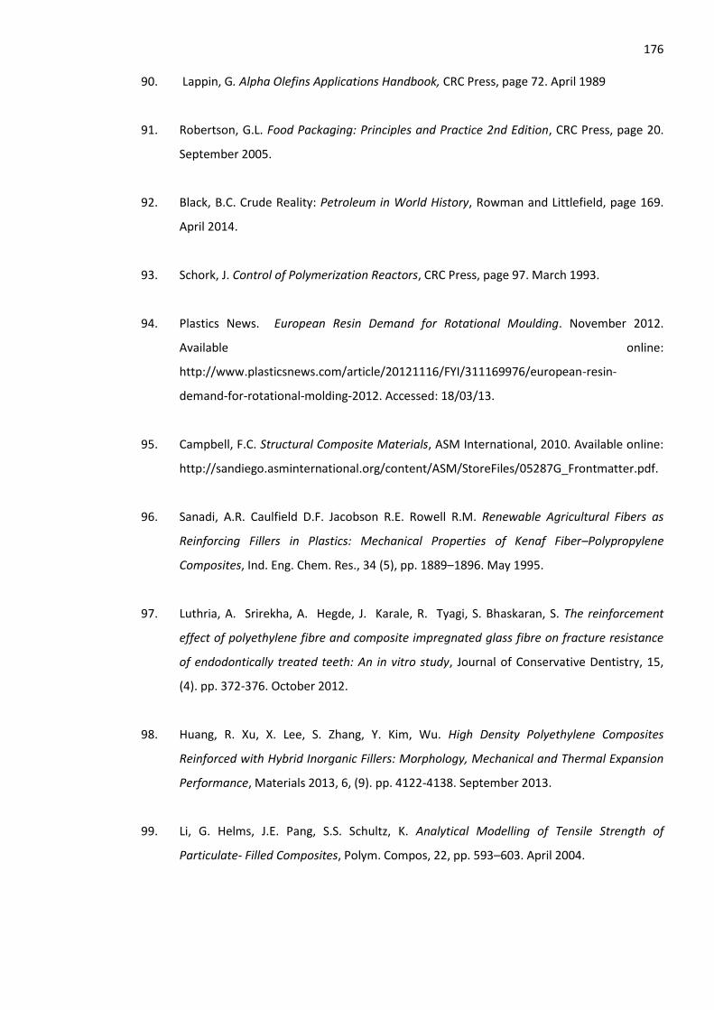
176 90. Lappin, G. Alpha Olefins Applications Handbook, CRC Press, page 72. April 1989

91. Robertson, G.L. Food Packaging: Principles and Practice 2nd Edition, CRC Press, page 20.

September 2005.

92. Black, B.C. Crude Reality: Petroleum in World History, Rowman and Littlefield, page 169.

April 2014.

93. Schork, J. Control of Polymerization Reactors, CRC Press, page 97. March 1993.

94. Plastics News. European Resin Demand for Rotational Moulding. November 2012.

Available online:

http://www.plasticsnews.com/article/20121116/FYI/311169976/european-resin-

demand-for-rotational-molding-2012. Accessed: 18/03/13.

95. Campbell, F.C. Structural Composite Materials, ASM International, 2010. Available online:

http://sandiego.asminternational.org/content/ASM/StoreFiles/05287G_Frontmatter.pdf.

96. Sanadi, A.R. Caulfield D.F. Jacobson R.E. Rowell R.M. Renewable Agricultural Fibers as

Reinforcing Fillers in Plastics: Mechanical Properties of Kenaf Fiber–Polypropylene

Composites, Ind. Eng. Chem. Res., 34 (5), pp. 1889–1896. May 1995.

97. Luthria, A. Srirekha, A. Hegde, J. Karale, R. Tyagi, S. Bhaskaran, S. The reinforcement

effect of polyethylene fibre and composite impregnated glass fibre on fracture resistance

of endodontically treated teeth: An in vitro study, Journal of Conservative Dentistry, 15,

(4). pp. 372-376. October 2012.

98. Huang, R. Xu, X. Lee, S. Zhang, Y. Kim, Wu. High Density Polyethylene Composites

Reinforced with Hybrid Inorganic Fillers: Morphology, Mechanical and Thermal Expansion

Performance, Materials 2013, 6, (9). pp. 4122-4138. September 2013.

99. Li, G. Helms, J.E. Pang, S.S. Schultz, K. Analytical Modelling of Tensile Strength of

Particulate- Filled Composites, Polym. Compos, 22, pp. 593–603. April 2004.

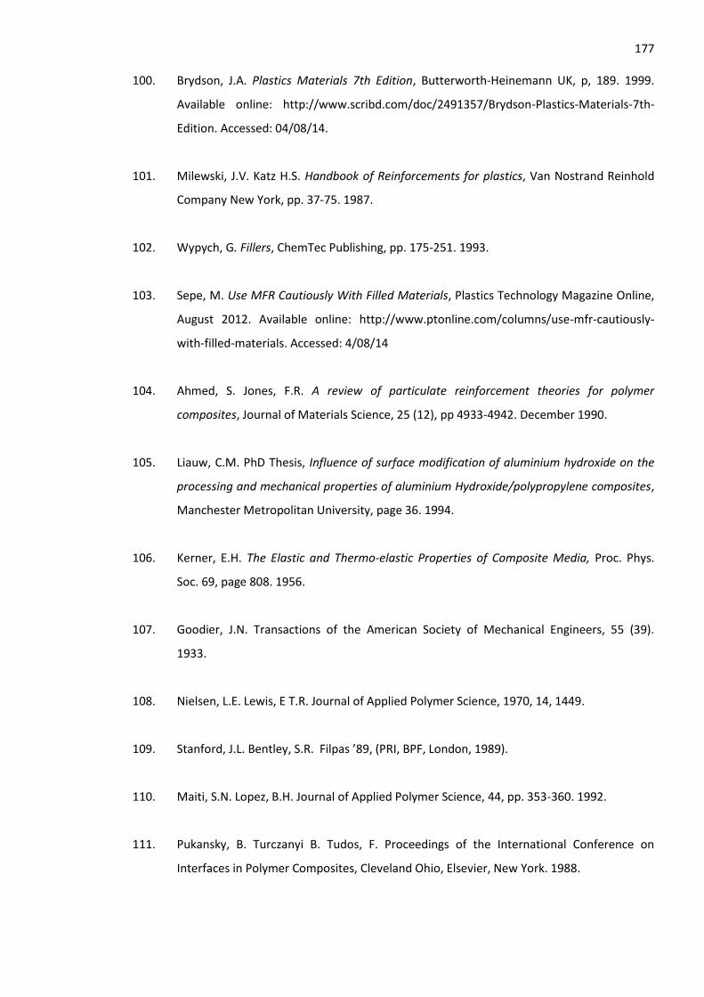
177 100. Brydson, J.A. Plastics Materials 7th Edition, Butterworth-Heinemann UK, p, 189. 1999.

Available online: http://www.scribd.com/doc/2491357/Brydson-Plastics-Materials-7th-

Edition. Accessed: 04/08/14.

101. Milewski, J.V. Katz H.S. Handbook of Reinforcements for plastics, Van Nostrand Reinhold

Company New York, pp. 37-75. 1987.

102. Wypych, G. Fillers, ChemTec Publishing, pp. 175-251. 1993.

103. Sepe, M. Use MFR Cautiously With Filled Materials, Plastics Technology Magazine Online,

August 2012. Available online: http://www.ptonline.com/columns/use-mfr-cautiously-

with-filled-materials. Accessed: 4/08/14

104. Ahmed, S. Jones, F.R. A review of particulate reinforcement theories for polymer

composites, Journal of Materials Science, 25 (12), pp 4933-4942. December 1990.

105. Liauw, C.M. PhD Thesis, Influence of surface modification of aluminium hydroxide on the

processing and mechanical properties of aluminium Hydroxide/polypropylene composites,

Manchester Metropolitan University, page 36. 1994.

106. Kerner, E.H. The Elastic and Thermo-elastic Properties of Composite Media, Proc. Phys.

Soc. 69, page 808. 1956.

107. Goodier, J.N. Transactions of the American Society of Mechanical Engineers, 55 (39).

1933.

108. Nielsen, L.E. Lewis, E T.R. Journal of Applied Polymer Science, 1970, 14, 1449.

109. Stanford, J.L. Bentley, S.R. Filpas ’89, (PRI, BPF, London, 1989).

110. Maiti, S.N. Lopez, B.H. Journal of Applied Polymer Science, 44, pp. 353-360. 1992.

111. Pukansky, B. Turczanyi B. Tudos, F. Proceedings of the International Conference on

Interfaces in Polymer Composites, Cleveland Ohio, Elsevier, New York. 1988.

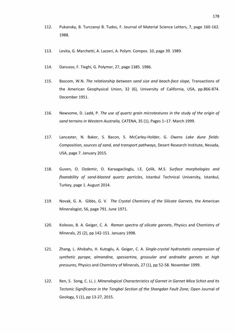
178 112. Pukansky, B. Turczanyi B. Tudos, F. Journal of Material Science Letters, 7, page 160-162.

1988.

113. Levita, G. Marchetti, A. Lazzeri, A. Polym. Compos. 10, page 39. 1989.

114. Danusso, F. Tieghi, G. Polymer, 27, page 1385. 1986.

115. Bascom, W.N. The relationship between sand size and beach-face slope, Transactions of

the American Geophysical Union, 32 (6), University of California, USA, pp.866-874.

December 1951.

116. Newsome, D. Ladd, P. The use of quartz grain microtextures in the study of the origin of

sand terrains in Western Australia, CATENA, 35 (1), Pages 1–17. March 1999.

117. Lancaster, N. Baker, S. Bacon, S. McCarley-Holder, G. Owens Lake dune fields:

Composition, sources of sand, and transport pathways, Desert Research Institute, Nevada,

USA, page 7. January 2015.

118. Guven, O. Ozdemir, O. Karaagaclioglu, I.E. Çelik, M.S. Surface morphologies and

floatability of sand-blasted quartz particles, Istanbul Technical University, Istanbul,

Turkey, page 1. August 2014.

119. Novak, G. A. Gibbs, G. V. The Crystal Chemistry of the Silicate Garnets, the American

Mineralogist, 56, page 791. June 1971.

120. Kolesov, B. A. Geiger, C. A. Raman spectra of silicate garnets, Physics and Chemistry of

Minerals, 25 (2), pp 142-151. January 1998.

121. Zhang, L. Ahsbahs, H. Kutoglu, A. Geiger, C. A. Single-crystal hydrostatic compression of

synthetic pyrope, almandine, spessartine, grossular and andradite garnets at high

pressures, Physics and Chemistry of Minerals, 27 (1), pp 52-58. November 1999.

122. Ren, S. Song, C. Li, J. Mineralogical Characteristics of Garnet in Garnet Mica Schist and Its

Tectonic Significance in the Tongbai Section of the Shangdan Fault Zone, Open Journal of

Geology, 5 (1), pp 13-27, 2015.

179 123. Durdzińskia, P. T. Dunanta, C. F. Hahab, M. B. Scrivenera, K.L. A New quantification

Method based on SEM-EDS to Assess Fly Ash Composition and Study the Reaction of its

Individual Components in Hydrating Cement Paste, Cement and Concrete Research, 73,

pp. 111-122. July 2015.

124. Divya, V.C. Khan, M. A. Rao, B. N. Sailaja, R.R.N. High-density Polyethylene/Cenosphere

Composites Reinforced with Multi-Walled Carbon Nanotubes: Mechanical, Thermal and

Fire Retardancy Studies, Materials and Design Journal, 65, pp. 377-386. 2015.

125. Yao, Z.T. Ji, X.S. Sarker, P.K. Tang, J.H. Ge, L.Q. Xia, M.S. Xi, Y.Q. A comprehensive review

on the applications of coal fly ash, Earth-Science Reviews, 141, pp. 105–121. 2015.

126. Feng, X. Clark, B. Evaluation of the Physical and Chemical Properties of Fly Ash Products

for Use in Portland Cement Concrete, 2011 World of Coal Ash conference, Denver, CO,

USA, page 6. May 2011.

127. Samuels, R.J. Structured Polymer Properties, Wiley, New York, 1974.

128. Gorrasi, G. Di Lieto, R. Patimo, G. De Pasquale, S. Sorrentino, A. Structure property

relationships on uniaxially oriented carbon nanotube/polyethylene composites, Polymer,

52, pp. 1124-1132. 2011.

129. Bilotti, E. Fischer, H. Peijs, R.T. Polymer Nanocomposites Based on Needle-like Sepiolite

Clays: Effect of Functionalized Polymers on the Dispersion of Nano filler, Crystallinity, and

Mechanical Properties, Queen Mary University of London, Journal of applied polymer

science 107 (2), pp. 1116-1123, January 2008.

130. Kendall, K. Interface Science and Composites, British Polymer Journal, 10, pp.35-38. 1978.

131. Wong, K. J. Yousif, B. F. Low, K. O. Ng, Y. Tan, S. L. Effects of fillers on the fracture

behaviour of particulate polyester composites, The Journal of Strain Analysis for

Engineering Design, 45 (1), pp. 67-78. January 2010.

132. Ribnikar, F. Journal of Applied Polymer Science, 42, pp. 2727-2732. 1991.

133. Kangoa, S. Kaliab, S. Celli, A. Njugunad, J. Habibie, Y. Kumara, R. Surface modification of

inorganic nanoparticles for development of organic–inorganic nanocomposites - A review,

180

Jaypee University of Information Technology, India, Progress in Polymer Science Journal

38 (4), pp. 421. April 2013.

134. Arnaud, R. PhD Thesis, An Investigation into the Effects of the Introduction of Fillers on the

Properties of Rotationally Moulded Products, Queens University Belfast, page 13.

September 1998.

135. Fu, S. Feng, X. Lauke, B. Mai, Y. Effects of particle size, particle/matrix interface adhesion

and particle loading on mechanical properties of particulate–polymer composites,

Technical Institute of Physics and Chemistry, Beijing, China, Composites Journal, Part B:

Engineering 39 (6), pp. 933–961. September 2008.

136. Schlumpf, H.P. Kuntstoffe, 73, pp. 511-515. 1983.

137. Vu-Kahn, T. Fisa, B. Polym. Compos, 7, pp. 219-226. 1986.

138. Riley, A.M. Paynter, C.D. McGenity P.M. Adams J.M. Factors affecting the impact

properties of mineral filled polypropylene, Plast. Rubber Proc. Applic. 14, pp. 85-93. 1990.

139. Trtignon, J.P. Verdu, J. De Bossard ,R. De Vallois, A. Polypropelene-Mica Composites,

Polym.Compos., Edited by Sedlacek B., Walter de Gruyter, Berlin, pp. 191-198. 1986.

140. Oey, T. Kumar, A. Bullard, J.W. Neithalath, N. Sant, G. The Filler Effect: The Influence of

Filler Content and Surface Area on Cementitious Reaction Rates, Journal of the American

Ceramic Society, 96 (6), pp. 1978-1990. June 2013.

141. Tanimoto, M. Yamagata, T. Miyata, K. Ando, S. Anisotropic Thermal Diffusivity of

Hexagonal Boron Nitride-Filled Polyimide Films: Effects of Filler Particle Size, Aggregation,

Orientation, and Polymer Chain Rigidity, Applied Materials and Interfaces, 5 (10), pp

4374–4382. 2013.

142. Liauw, C.M. Lees, G.C. Rothon, R.N. Voliotis, A. Wild, F. Sunderland, P. Schofield, J.

Thetford, D. Evolution of reactive unsaturated interfacial modifiers for polyolefin based

composites, Composite Interfaces, 13(8-9) p. 717-736. 2006.

181 143. Fernandes, E.M. Correlo, V.M. Mano, J. F. Reis, R. L. Novel cork–polymer composites

reinforced with short natural coconut fibres: Effect of fibre loading and coupling agent

addition, University of Minho, Portugal, Composites Science and Technology Journal 78,

pp. 56–62. 2013.

144. Jaehyung, J. Morgan, R.J. Interfacial Failure of Composites at Cryogenic and Elevated

Temperatures, Texas A&M University, NASA Glenn Research Centre Cleveland, USA,

Society of Plastics Engineers ANTEC (Annual Technical) Conference Proceedings, page 1.

2006.

145. Vautarda, F. Fiouxa, P. Vidala, L. Schultza, J. Nardina, M. Defoort, B. Influence of the

carbon fiber surface properties on interfacial adhesion in carbon fiber–acrylate composites

cured by electron beam, Composites Part A: Applied Science and Manufacturing, 42 (7),

pp. 859-867. July 2011.

146. Wang, H.W. Zhou, H.W Peng, R.D. Mishnaevsky, L. Nanoreinforced polymer composites:

3D FEM modeling with effective interface concept, Composites Science and Technology,

71 (7), pp. 980-988. May 2011.

147. Vollenberg, P.H.T. Heikens, D. Polymer, 30, pp.1656-1662. 1989.

148. Maiti, S.N. Mahahapatro P.K. Journal of Applied Polymer Science, 42, pp. 3101-3110. 1991.

149. Yanjun, X. Callum, A.S. Hill. Zefang B.X. Militz. H. Carsten M. Silane coupling agents used

for natural fiber/polymer composites: A review, Edinburgh Napier University, Composites :

Part A (41), Journal, pp. 806–819. 2010.

150. Mahouche-Chergui, S. Gam-Derouich, S. Mangeney, C. Chehimi, M.M. Aryl, diazonium

salts: a new class of coupling agents for bonding polymers, biomacromolecules and

nanoparticles to surfaces, Chemical Society Reviews, 40, pp. 4143-4166. 2011.

151. Bluemmel, P. Setaro, A. Popeney, C.S. Haag, R. Reich, S. Dispersion of carbon nanotubes

using an azobenzene derivative, physica status solidi, 247 (11-12), pp. 2891-2894,

December 2010.

182 152. Liauw, C.M. Hurst S.J. Lees G.C. Rothon R.N. Dobson D.C. The effect of filler surface

modification on the mechanical properties of aluminium hydroxide filled polypropylene.

Plastics Rubber and Composites Processing and Applications, 24 (5), p. 249-260. 1995.

153. Pukánszky, B. Influence of interface interaction on the ultimate tensile properties of

polymer composites, Composites, 21 (3), pp. 255–262. May 1990.

154. Brechet, Y. Polymer Based Nanocomposites: Effect of Filler-Filler and Filler-Matrix

Interactions, Advanced Engineering Materials, 3 (8), 2001.

155. Bernada, A.C. Fibre Glass Reinforced HDPE, SPE Journal, 26, pp. 37-45. October 1970.

156. Kalia, S. Kaith B.S. Kaur I. Pre-treatments of Natural Fibers and their Application as

Reinforcing Material in Polymer Composites - A Review, Polymer Engineering and Science,

49 (7), pp.1253-1272. March 2009.

157. Trivedi, B.C. Culbertso B.M. Maleic anhydride, Plennum Press, New York-London, pp. 459-

462. 1981.

158. Marti, L.W. Overview of Maleic Anhydride Grafted Polyolefin Coupling Agents – A Guide to

Understanding their Uses, Benefits, Functions, Selections and Development. ADDCOMP.

(no date). Available online:

http://www.speautomotive.com/SPEA_CD/SPEA2012/pdf/TP/TP9.pdf. Accessed::

01/04/2012.

159. Shih, R.H. Introduction to Finite Element Analysis Using Creo Simulate 1.0, SDC

Publications, page 2. 2011.

160. Novak, M. Dolsak B. Intelligent FEA-based design improvement, Engineering Applications

of Artificial Intelligence, 21. pp. 1239-1254. December 2008.

161. Haghighi, K. Finite Element Method (FEM/FEA) Introduction, University of Purdue, Indiana,

USA, page 3. January 2001. Available online:

https://engineering.purdue.edu/~abe601/lecture/Introduction.pdf Accessed: 25/06/14.

183 162. Burkhart, D. Hamann, B. Umlauf, G. Finite Element Analysis for Linear Elastic Solids Based

on Subdivision Schemes, University of Kaiserslautern, Germany and University of

California, USA. March 2010.

163. M.S. Gockenbach, Understanding and implementing the finite element method, Society

for Industrial and Applied Mathematics (SIAM), January 1987.

164. Agarwal, R. B. Introduction to Finite Element Analysis: An Overview of the Finite Element

Analysis, San Jose State University, August 2002.

165. Wang, W. Sadeghipour, K. Baran, G. Finite element analysis of the effect of an interphase

on toughening of a particle-reinforced polymer composite, Composites: Part A, 39, (6). pp.

956–964. June 2008.

166. Pesaran, A.A. Kim, G.H. Smith, K. Santhanagopalan, S and Lee, K..J. Computer-Aided

Engineering for Electric Drive Vehicle Batteries, Lee National Renewable Energy

Laboratory, Colorado, USA. May 2011. Available online:

http://www.nrel.gov/vehiclesandfuels/energystorage/pdfs/50914.pdf. Accessed:

05/08/14.

167. Drai, A. Aour, B. Analysis of the temperature effect on the behaviour of high density

polyethylene during high pressure torsion process, 21ème Congrès Français de Mécanique

proceedings, 26 August 2013.

168. Cailletaud, G. El Arem, S. Introduction to Finite Element Method, ParisTech Institute of

Science and Technology Materials Centre. June 2010. Available online:

http://mms2.ensmp.fr/tribo_paris/lectures/Introduction_FE.pdf Accessed: 4/08/14.

169. Kersale, E. Analytic Solutions of Partial Differential Equations, School of Mathematics,

University of Leeds. September 2009. Available online:

http://www1.maths.leeds.ac.uk/~kersale/Teach/M3414/Notes/m3414_1.pdf. Accessed:

09/06/14.

170. Ames, W.F. Numerical Methods for Partial Differential Equations, Academic Press, page 1.

June 2014.

184 171. Churchill, R. C. and Kovacic, J. J. Introduction to Differential Galois Theory, page 3. 2006.

Available online: http://www.sci.ccny.cuny.edu/~ksda/PostedPapers/intro.pdf Accessed:

07/05/2015.

172. Maes, M. Huyse, L., Reliability and Optimization of Structural Systems, Proceedings of the

11th IFIP WG7.5 Working Conference, CRC Press, page 276. July 2004.

173. Cajori, F. The Early History of Partial Differential Equations and of Partial Differentiation

and Integration, American Mathematical Monthly, 35 (9). November 1928.

174. Courant, R. Friedrichs, K. Lewy, H. Partial Difference Equations of Mathematical Physics,

Mathematische Annalen, 100, (1). pp. 32-74. 1928.

175. Williamson, F. Richard Courant and the Finite Element Method: A Further Look, Historia

Mathematica 7, (4). November 1980, pp. 369–378.

176. Courant, R. Variational methods for the solution of problems of equilibrium and

vibrations, Bull. Amer. Math. Soc., 49. pp. 1-23. 1943

177. Hart, V. G. The Hypercircle and J.L. Synge, Mathematical Proceedings of the Royal Irish

Academy, 107, (2). pp.153-161. January 2007.

178. Felippa, C. The Origins of the Finite Element Method. University of Colorado, USA August

2013. Available online: http://home.iitk.ac.in/~mohite/History_of_FEM.pdf Accessed:

05/08/14.

179. Heyman, J. Structural Analysis: A Historical Approach, Cambridge University Press, May

1998.

180. Turner, M. J. Clough, R. Martin, W. H. C. Topp, L. J. Stiffness and Deflection of Complex

Structures, Journal of Aeronautical Sciences, 23, (9). pp. 805-824. September 1956.

181. Kurrer, K. The History of the Theory of Structures: From Arch Analysis to Computational

Mechanics, John Wiley and Sons Inc., January 2012.

182. Ortiz M. Computational micromechanics, Computational Mechanics, 18, (5). pp. 321-338.

September 1996.

185 183. A.F. Bower, Applied Mechanics of Solids Chapter 8: Theory and Implementation of the

finite element method. Available online:

http://solidmechanics.org/text/Chapter8_1/Chapter8_1.htm Accessed: 25/04/2015.

184. Boeraeve, P. Introduction to the finite element method, Gramme Institute, Angleur,

Belgium, page 62. 2010. Available online:

http://www.gramme.be/unite9/FEM/Finite%20Element%20Method.pdf Accessed:

29/04/2015.

185. Hibbit, H. D. Marcal, P. V. Rice, J. R. A Finite Element Formulation for Problems of Large

Strain and Large Displacement, International Journal of Solid Structures, 6, Pergamon

Press, pp. 1069 to 1086. 1970.

186. Huebner, K. H. The Finite Element Method for Engineers, John Wiley & Sons, page 668,

September 2001.

187. Reddy, J. N. An Introduction to Nonlinear Finite Element Analysis: with applications to heat

transfer, fluid mechanics, and solid mechanics, Oxford University Press, page 83. October

2014.

188. Farmaga, I. Shmigelskyi, P. Spiewak, P. Ciupinski, L. Evaluation of Computational

Complexity of Finite Element Analysis, CAD Systems in Microelectronics (CADSM). pp.213-

214. February 2011

189. Vicich, B. Ryan, C. Meredith, K. Linear vs. Nonlinear Contact Analysis, Samtec Inc., 2007.

Available online:

https://www.samtec.com/documents/webfiles/technical_library/reference/articles/linea

r_vs_%20non-linear_contact_analysis_082207.pdf. Accessed: 05/08/14.

190. Shahidi, Y.K. Article. Key Assumptions in FEA for Design, January 2010. Available online:

http://engineering-inventions.blogspot.co.uk/2010/01/key-assumptions-in-fea-for-

design.html Accessed: 26/06/14.

191. Ivančo, V. Nonlinear Finite Element Analysis, Faculty of Mechanical Engineering,

Technical University of Košice, Slovakia. June 2011. Available online: http://www.mb.hs-

186

wismar.de/~heinze/subdir/FEA_of_Nonlinear_Problems_2011_Ivanco.pdf. Accessed:

05/08/14.

192. Felippa, C. A Tour of Nonlinear Analysis, August 2013. University of Colorado, USA, August

2013. Page 12 Available online:

http://www.colorado.edu/engineering/CAS/courses.d/NFEM.d/NFEM.Ch02.d/NFEM.Ch0

2.pdf. Accessed: 05/08/14.

193. Prasad, N.P. Introduction to Nonlinear Optical Effects in Molecules and Polymers, Wiley

and Sons. January 1991.

194. Dassault Systemes. Understanding Nonlinear Analysis, page 4. March 2010. Available

online:

http://files.solidworks.com/whitepapers/2010/Nonlinear_Analysis_2010_ENG_FINAL.pdf.

Accessed: 05/08/14.

195. McHugh, P. Non-Linear Finite Element Analysis: Finite Element Solution Schemes I and II,

Department of Mechanical and Biomedical Engineering, University of Ireland, 2007.

Available online:

http://www.nuigalway.ie/micru/Non%20Linear%20Finite%20Element%20Methods.pdf.

Accessed: 05/08/14.

196. Bonet, J. Wood, D.R. Nonlinear Continuum mechanics for Finite Element Analysis,

Cambridge University Press, 1997.

197. Dolšak, B. Finite element mesh design expert system, Knowledge-Based Systems 15, (5),

pp. 315-322. July 2002.

198. Shengwei, M. Article. Top 5 misunderstandings on (good) mesh, October 2011. Available

online: http://caewatch.com/top-5-misunderstandings-on-good-mesh/. Accessed:

05/08/14.

199. Behrens, J. Beisiegel, N. Pranowo, W. Inundation modelling with adaptive triangular

mesh refinement - state of the art numerical methods for accurate simulation, University

of Hamburg. September 2010. Available online:

187

http://www.loicz.org/imperia/md/content/loicz/stormsurges/posterd/p41_beispiegel_et

al.pdf. Accessed: 05/08/14.

200. Babuvška I. Rheinboldt W. C. Error Estimates for Adaptive Finite Element Computations,

SIAM Journal on Numerical Analysis, 15, (4). pp. 736-754. 1978

201. Li, Y. Premasuthan, S. Jameson, A. Comparison of h- and p- Adaptations for Spectral

Difference Methods, Aeronautics and Astronautics Department, Stanford University,

California, USA. July 2010.

202. Babuska, M. S. The P and H-P Versions of the Finite Element Method, Basic Principles and

Properties, SIAM Journal, 36, 4. pp. 578-632. December 1994.

203. Hodohara ,T. Finite Element Mesh Using h-refinement Procedure, Chuo University, Faculty

of Science and Engineering, Tokyo, Japan. October 2002.

204. Fiedler, G. Triangle subdivision, (no date) Available online:

http://gafferongames.com/virtualgo/tessellating-the-go-stone/. Accessed: 05/08/14.

205. Meschke, G. Finite Element Methods In Linear Structural Mechanics: Short Presentation in

Adaptive Finite Element, Ruhr University, Germany. February 2009. Available online:

http://www.sd.rub.de/downloads/Adaptive_Finite_Element_Methods. Accessed:

05/08/14.

206. Byfut, A. Schroder, A. hp–Adaptive Extended Finite Element Method, International Journal

for Numerical Methods in Engineering, 89, 11, pp. 1392–1418. March 2012.

207. McRae, D. S. r-Refinement grid adaptation algorithms and issues, Department of

Mechanical and Aerospace Engineering, North Carolina State University, USA. May 1999.

208. Kuo, Y.L. Cleghorn, W.L. Behdinan, K. Fenton, R.G. The h–p–r-refinement finite element

analysis of a planarhigh-speed four-bar mechanism, Department of Mechanical and

Industrial Engineering, University of Toronto, Ontario, Canada. September 2005.

209. Kuo, Y. L. Cleghorn W. L The h-, p-, and r-refinements of Finite Element Analysis of Flexible

Slider Crank Mechanism, Journal of Vibration and Control, 13.pp. 415-435. April 2007.

188 210. Maddi, J.R. Vable, M. An hpr-mesh refinement algorithm for BEM, Engineering Analysis

with Boundary Elements, 34. pp. 549-556. January 2010.

211. Maurer, D. Image. P-Refinement of a Finite Element Mesh. University of Landshut Applied

Sciences, (no date). Available online: https://people.fh-

landshut.de/~maurer/femeth/node271.html. Accessed: 05/08/14

212. Kingspan vs Borealis County Court Judgement. London Royal Courts of Justice. May 2012.

Available online:

http://www.7kbw.co.uk/media/uploaded_files/Kingspan_v_Borealis_Final.pdf. Accessed:

04/08/14.

213. Goldstein, J. Newbury, D.E. Joy, D.C. Lyman, C.E. Echlin, P. Lifshin, E. Sawyer, L. Michael,

J.R. Scanning Electron Microscopy and X-ray Microanalysis: Third Edition, Springer Science

& Business Media, page 1. December 2012.

214. Schroder, D.K. Semiconductor Material and Device Characterization, John Wiley & Sons,

page 631. February 2006.

215. Goodhew, P.J. Humphreys, J. Beanland, R. Electron Microscopy and Analysis Third Edition,

CRC Press, page 125. November 2000.

216. Khursheed, A. Scanning Electron Microscope Optics and Spectrometers, World Scientific,

page 3. 2011.

217. Brundle, C. R. Baker, A.D. Electron Spectroscopy Volume 3, Academic Press, page 23. 1979.

218. Brundle, C. R. Evans, C.A. Wilson, S. Encyclopedia of Materials Characterization: Surfaces,

Interfaces, Thin Films, Gulf Professional Publishing, page 122. 1992.

219. Lawson, G. Chemical Analysis of Polymers, iSmithers Rapra Publishing, page 18. December

1991.

220. Höhne, G. Hemminger, W. Flammersheim, H-J. Differential Scanning Calorimetry,

Springer Science & Business Media, page 1. July 2003.

189 221. Sepe, M.P. Thermal Analysis of Polymers, iSmithers Rapra Publishing, page 3. January

1997.

222. Wunderlich, B. Macromolecular Physics, 1, Academic Press, New York, chapter 3. 1973.

223. Crompton, T.R. Polymer Reference Book, iSmithers Rapra Publishing, page 437. January

2006.

224. Wunderlich, B. Cormier, C. M. Heat of fusion of polyethylene, Journal of Polymer Science

Part A-2: Polymer Physics, 5(5), John Wiley and Sons Inc., September 1967.

225. Studies and Information Services, Committee on Aeronautics Research and Technology

for Vision 2050, Aeronautics and Space Engineering Board, Transportation Research

Board, Division on Engineering and Physical Sciences, National Research Council. Securing

the Future of U.S. Air Transportation: A System in Peril, National Academies Press, page

23. November 2003.

226. Potgieter, H. Liauw, C.M. Velado, D. Effect of Fly Ash Washing Conditions on the Properties

of Coupling Agent Modified Polypropylene/Fly Ash Composites, Polymer Composites, 35

(4). April 2014.

227. Srivatsan, T. S. Bhatnagar, N. Processing and Fabrication of Advanced Materials XVII Part

8, Polymer-based composites and nano composites Volume Two, I. K. International Pvt

Ltd., page 481. 2009.

228. Rothon, R. Particulate-filled Polymer Composites, iSmithers Rapra Publishing, page 19.

January 2003.

229. Nurshamila, S.B. Ismail, H. Othman, N. The effects of Rattan Filler Loading on the

Properties of Rattan Powder-Fillled Polyproperlene Composites. Bioresources Journal, 7(4),

pp.5677-5690. 2012.

230. Deepthi, M.V. Sharma, M. Sailaja, R.R.N. Anantha, P. Sampathkumaran, P. Seetharamu,

S. Mechanical and thermal characteristics of high density polyethylene–fly ash

Cenospheres composites, Materials and Design, 31, pp.2051-2060. 2010.

231. Fanderlik, I. Silica Glass and Its Application, Elsevier, page 208. October 2013.

190 232. Whitney, D. L. Broz, M. Cook, R.F. Hardness, toughness, and modulus of some common

metamorphic minerals, American Mineralogist, 92 (2), pp. 281-288. 2007.

233. Dong, M. Li, S. Xie, J. Han, J. Experimental Studies on the Normal Impact of Fly Ash

Particles with Planar Surfaces, Energies 2013, 6(7), pp. 3245-3262. July 2013.

234. Okiyokota, M. Fracture Behaviour of Fiber Reinforced PPS Injection Moulding, Society of

Plastics Engineer ANTEC (Annual Technical) Conference Proceedings, CRC Press, page

3320. April 1997.

235. Hosford, W. F. Solid Mechanics, Cambridge University Press, page 7. March 2010.

236. Yoo, Y. Spencer, M.W. Paul, D.R. Morphology and mechanical properties of glass fiber

reinforced Nylon 6 nanocomposites, Polymer, 52, pp. 180-190. 2011.

237. Yoo, M. Masters Thesis, Comparison of Interlaminar Fracture Toughening of Filament

Wound Glass/Epoxy Composites by Using MWCNT’s or Flexible Resin, The Pennsylvania

State University Graduate School, Department of Aerospace Engineering, page 7. August

2009.

238. Bashar, M. Sundararaj, U. Mertiny, P. Study of matrix micro-cracking in nano clay and

acrylic tri-block-copolymer modified epoxy/basalt fiber-reinforced pressure-retaining

structures, eXPRESS Polymer Letters, 5 (10), pp. 882–896. April 2011.

239. Friedrich, K. Fakirov, S. Zhang, Z. Polymer Composites: From Nano- to Macro-Scale,

Springer Science & Business Media, page 52. July 2005.

240. Hassan, A. Abdul Rahman, N. Yahya, R. Extrusion and Injection-Molding of Glass

Fiber/MAPP/Polypropylene: Effect of Coupling Agent on DSC, DMA and Mechanical

Properties, Journal of Reinforced Plastics and Composites, page 1. September 2011.

241. Petchwattana, N. Covavisaruch, S. Chanakul, S. Mechanical properties, thermal

degradation and natural weathering of high density polyethylene/rice hull composites

compatibilized with maleic anhydride grafted polyethylene, Journal of Polymer Research,

19 (9921), page 4. June 2012.

191 242. Kord, B. Influence of Maleic Anhydride on the Flexural, Tensile and Impact Characteristics

of Sawdust Flour Reinforced Polypropylene Composite, World Applied Sciences Journal, 12

(7), pp. 1014-1016, 2011.

243. Swallowe, G.M. Mechanical Properties and Testing of Polymers: An A-Z Reference,

Springer Science & Business Media, page 134. November 1999.

244. Barbero, E.J. Finite Element Analysis of Composite Materials Using ANSYS® 2nd Edition,

CRC Press, page 24. December 2013.

245. Fathi, J. Ashrafi, S. Movla, H. Sobhaian, S. A novel method to determine Poisson’s ratio by

beta-ray absorption experiment, Elsevier Ltd. January 2012.

246. Lee, J. Lee, S, Chang, J. Thompson, M.S. Kang, D. Park, S. A Novel Method for the Accurate

Evaluation of Poisson’s Ratio of Soft Polymer Materials, The Scientific World Journal

(2013), published under the Creative Commons Attribution License. March 2013.

247. Priego-Capote, F. M.D. Luque-de-Castro, Analytical Applications of Ultrasound, Elsevier

Ltd., page 354. February 2007.

248. Bhabha, H. Liauw, C.M. Henwood, N.G. Taylor, H. Condliffe, J. Critical Factors Affecting the

Use of Finite Element Analysis For Rotomoulded Parts, Manchester Metropolitan

University, Manchester, UK, Rotomotive Ltd., Northampton, UK, Society of Plastics

Engineers ANTEC (Annual Technical) Conference Proceedings. April 2014.

249. Nicholson, D.W. Finite Element Analysis: Thermomechanics of Solids 2nd Edition, CRC

Press, page 342. April 2008.

250. Lai, J. Bakker, A. Polymer Engineering and Science, 35 (17). pp. 1339-1347. 1995.

192

Appendix 1

A list of twin screw extrusion and two roll mill compounds is provided. The relevant Results and

Discussion Sections and table numbers have been included for ease of reference to the thesis.

5.2 Characterisation of Materials for Composite Development

5.2.2 Dual polyethylene blends

5.2.2.2 Twin screw extrusion compounded formulations

Table 6. Combinations of MA-g-LLDPE with HDPE.

MA-g-LLDPE

(% wt.)

HDPE

(% wt.)

0 100

7.5 92.5

15 85

25 75

50 50

75 25

100 0

5.4 Comparison of Composite Formation Processes for Large Particle Composites (Dry Blending

of Pre-Mix versus Two Roll Mill Melt Blending and Moulding)

Table 10. Blend details of two roll milled and dry blended composites.

MA-g-LLDPE/LMDPE

(% wt.)

Filler

(% wt.)

100 0

75 25

50 50

40 60

30 70

25 75

20 80

15 85

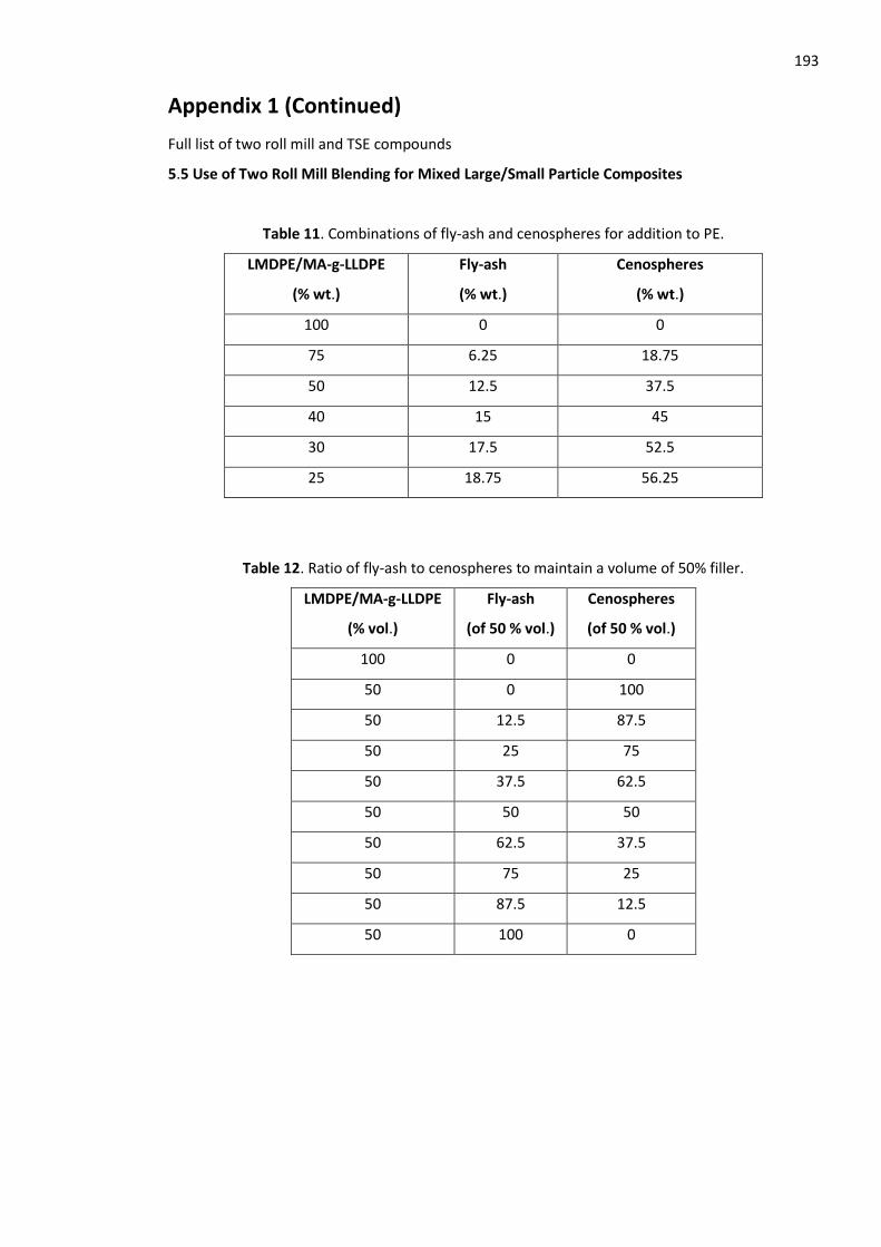
193

Appendix 1 (Continued)

Full list of two roll mill and TSE compounds

5.5 Use of Two Roll Mill Blending for Mixed Large/Small Particle Composites

Table 11. Combinations of fly-ash and cenospheres for addition to PE.

LMDPE/MA-g-LLDPE

(% wt.)

Fly-ash

(% wt.)

Cenospheres

(% wt.)

100 0 0

75 6.25 18.75

50 12.5 37.5

40 15 45

30 17.5 52.5

25 18.75 56.25

Table 12. Ratio of fly-ash to cenospheres to maintain a volume of 50% filler.

LMDPE/MA-g-LLDPE

(% vol.)

Fly-ash

(of 50 % vol.)

Cenospheres

(of 50 % vol.)

100 0 0

50 0 100

50 12.5 87.5

50 25 75

50 37.5 62.5

50 50 50

50 62.5 37.5

50 75 25

50 87.5 12.5

50 100 0

194

Appendix 1 (Continued)

5.6 Evaluation of Twin Screw Extrusion Compounding for Production of Small Particle

Composites

Table 13. Fly-ash and maleanised PE combinations for twin screw extrusion compounding.

MA-g-LLDPE/LMDPE

(% wt.)

Fly-ash

(% wt.)

100 0

75 25

50 50

40 60

30 70

25 75

5.7 Verification of Maleic Anhydride Coupling Agent Effect on Small Particle Composites

Produced by Twin Screw Extrusion Compounding

Table 14. Fly-ash analogue PE combinations investigated.

Analogue PE

(% wt.)

Fly-ash.

(% wt.)

100 0

75 25

50 50

40 60

30 70

25 75

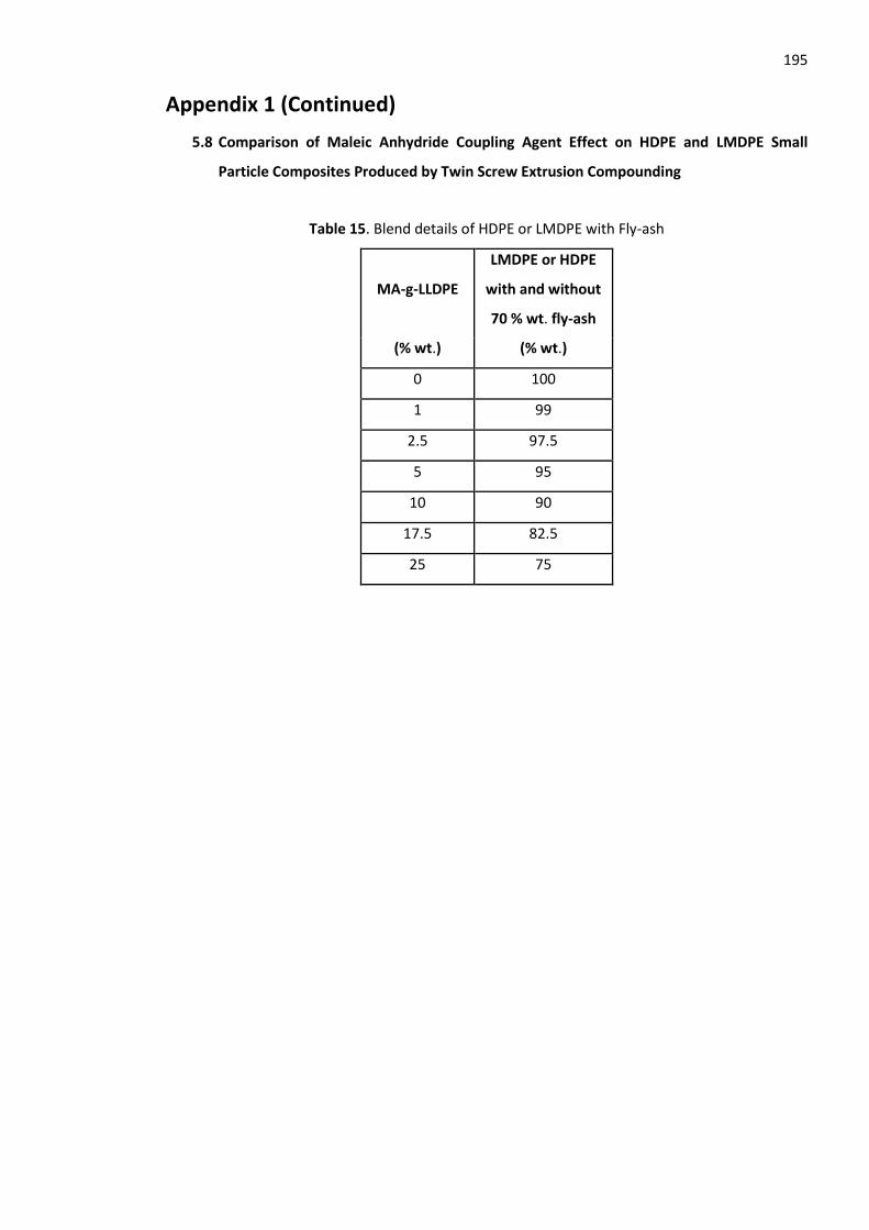
195

Appendix 1 (Continued)

5.8 Comparison of Maleic Anhydride Coupling Agent Effect on HDPE and LMDPE Small

Particle Composites Produced by Twin Screw Extrusion Compounding

Table 15. Blend details of HDPE or LMDPE with Fly-ash

MA-g-LLDPE

LMDPE or HDPE

with and without

70 % wt. fly-ash

(% wt.) (% wt.)

0 100

1 99

2.5 97.5

5 95

10 90

17.5 82.5

25 75

196

Appendix 1 (Continued)

5.9 Analysis of Rotationally Moulded Small Particle Composites

5.9.1 Rotomoulded rectangular box test mouldings

Table 16. Small Rectangular Box Mouldings

MA-g-

LLDPE/LMDPE

(% wt.)

Fly-ash.

(% wt.)

100 0

75 25

50 50

40 60

30 70

5.9.2 Rotomoulded safety steps

Table 18. PE/fly-ash formulations for rotomoulded safety steps.

Target Wall Thickness

(mm)

MA-g-LLDPE/LMDPE

(% wt.)

Fly-ash

(% vol.)

Fly-ash

(% wt.)

7 50 28.8 50

7 75 14.4 25

7 87.5 7.2 12.5

7 100 0 0

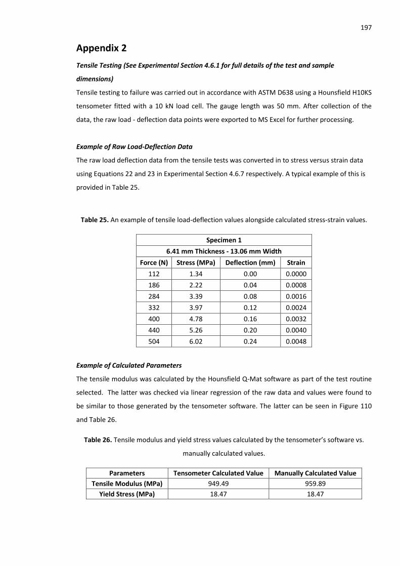
197

Appendix 2

Tensile Testing (See Experimental Section 4.6.1 for full details of the test and sample

dimensions)

Tensile testing to failure was carried out in accordance with ASTM D638 using a Hounsfield H10KS

tensometer fitted with a 10 kN load cell. The gauge length was 50 mm. After collection of the

data, the raw load - deflection data points were exported to MS Excel for further processing.

Example of Raw Load-Deflection Data

The raw load deflection data from the tensile tests was converted in to stress versus strain data

using Equations 22 and 23 in Experimental Section 4.6.7 respectively. A typical example of this is

provided in Table 25.

Table 25. An example of tensile load-deflection values alongside calculated stress-strain values.

Specimen 1

6.41 mm Thickness - 13.06 mm Width

Force (N) Stress (MPa) Deflection (mm) Strain

112 1.34 0.00 0.0000

186 2.22 0.04 0.0008

284 3.39 0.08 0.0016

332 3.97 0.12 0.0024

400 4.78 0.16 0.0032

440 5.26 0.20 0.0040

504 6.02 0.24 0.0048

Example of Calculated Parameters

The tensile modulus was calculated by the Hounsfield Q-Mat software as part of the test routine

selected. The latter was checked via linear regression of the raw data and values were found to

be similar to those generated by the tensometer software. The latter can be seen in Figure 110

and Table 26.

Table 26. Tensile modulus and yield stress values calculated by the tensometer’s software vs.

manually calculated values.

Parameters Tensometer Calculated Value Manually Calculated Value

Tensile Modulus (MPa) 949.49 959.89

Yield Stress (MPa) 18.47 18.47

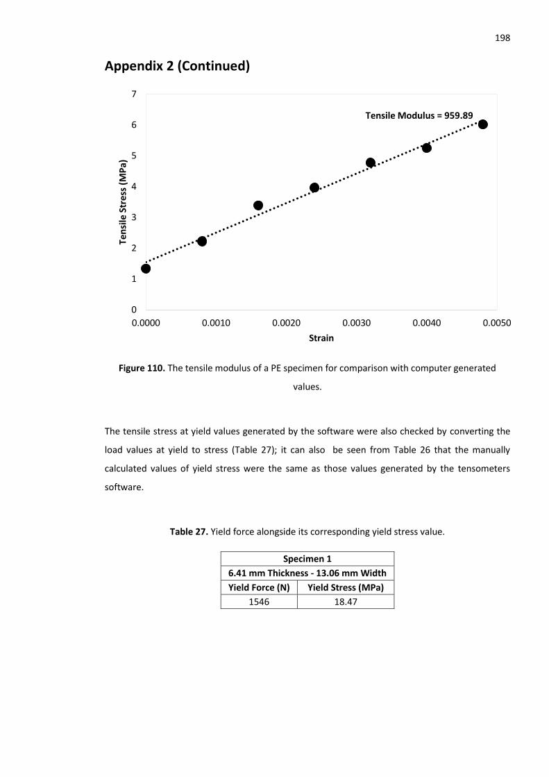
198

Appendix 2 (Continued)

Figure 110. The tensile modulus of a PE specimen for comparison with computer generated

values.

The tensile stress at yield values generated by the software were also checked by converting the

load values at yield to stress (Table 27); it can also be seen from Table 26 that the manually

calculated values of yield stress were the same as those values generated by the tensometers

software.

Table 27. Yield force alongside its corresponding yield stress value.

Specimen 1

6.41 mm Thickness - 13.06 mm Width

Yield Force (N) Yield Stress (MPa)

1546 18.47

Tensile Modulus = 959.89

0

1

2

3

4

5

6

7

0.0000 0.0010 0.0020 0.0030 0.0040 0.0050

Ten

sile

Str

ess

(MP

a)

Strain

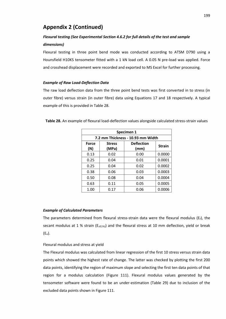
199

Appendix 2 (Continued)

Flexural testing (See Experimental Section 4.6.2 for full details of the test and sample

dimensions)

Flexural testing in three point bend mode was conducted according to ATSM D790 using a

Hounsfield H10KS tensometer fitted with a 1 kN load cell. A 0.05 N pre-load was applied. Force

and crosshead displacement were recorded and exported to MS Excel for further processing.

Example of Raw Load-Deflection Data

The raw load deflection data from the three point bend tests was first converted in to stress (in

outer fibre) versus strain (in outer fibre) data using Equations 17 and 18 respectively. A typical

example of this is provided in Table 28.

Table 28. An example of flexural load-deflection values alongside calculated stress-strain values

Specimen 1

7.2 mm Thickness - 10.93 mm Width

Force (N)

Stress (MPa)

Deflection (mm)

Strain

0.13 0.02 0.00 0.0000

0.25 0.04 0.01 0.0001

0.25 0.04 0.02 0.0002

0.38 0.06 0.03 0.0003

0.50 0.08 0.04 0.0004

0.63 0.11 0.05 0.0005

1.00 0.17 0.06 0.0006

Example of Calculated Parameters

The parameters determined from flexural stress-strain data were the flexural modulus (Ef), the

secant modulus at 1 % strain (Esf(1%)) and the flexural stress at 10 mm deflection, yield or break

(Eσ).

Flexural modulus and stress at yield

The Flexural modulus was calculated from linear regression of the first 10 stress versus strain data

points which showed the highest rate of change. The latter was checked by plotting the first 200

data points, identifying the region of maximum slope and selecting the first ten data points of that

region for a modulus calculation (Figure 111). Flexural modulus values generated by the

tensometer software were found to be an under-estimation (Table 29) due to inclusion of the

excluded data points shown in Figure 111.

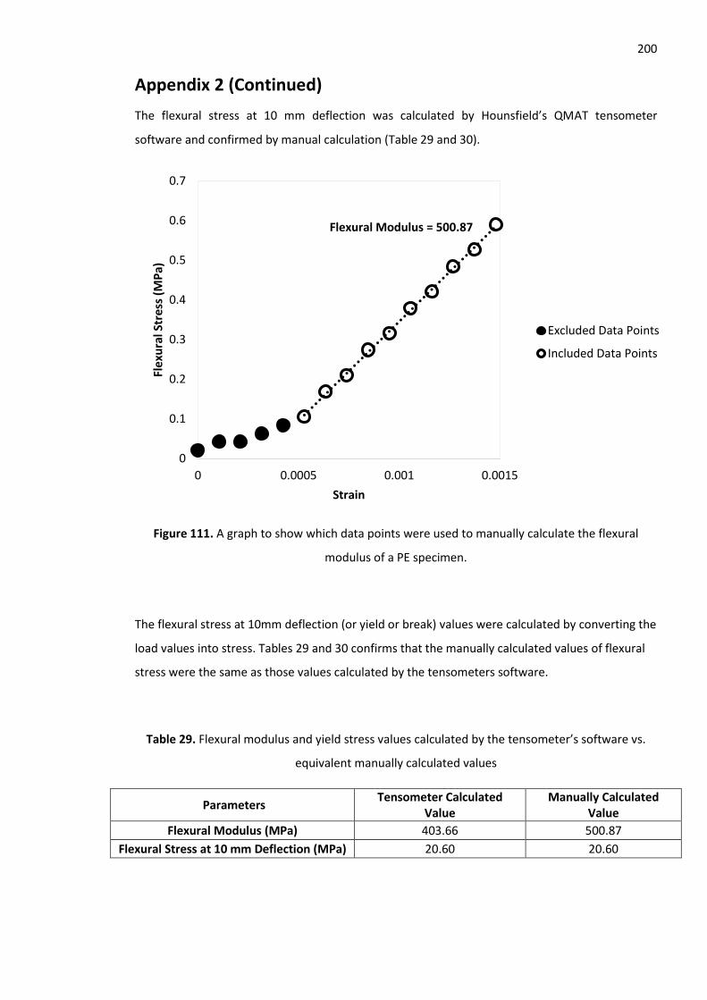
200

Appendix 2 (Continued)

The flexural stress at 10 mm deflection was calculated by Hounsfield’s QMAT tensometer

software and confirmed by manual calculation (Table 29 and 30).

Figure 111. A graph to show which data points were used to manually calculate the flexural

modulus of a PE specimen.

The flexural stress at 10mm deflection (or yield or break) values were calculated by converting the

load values into stress. Tables 29 and 30 confirms that the manually calculated values of flexural

stress were the same as those values calculated by the tensometers software.

Table 29. Flexural modulus and yield stress values calculated by the tensometer’s software vs.

equivalent manually calculated values

Parameters Tensometer Calculated

Value Manually Calculated

Value

Flexural Modulus (MPa) 403.66 500.87

Flexural Stress at 10 mm Deflection (MPa) 20.60 20.60

Flexural Modulus = 500.87

0

0.1

0.2

0.3

0.4

0.5

0.6

0.7

0 0.0005 0.001 0.0015

Fle

xura

l Str

ess

(MP

a)

Strain

Excluded Data Points

Included Data Points

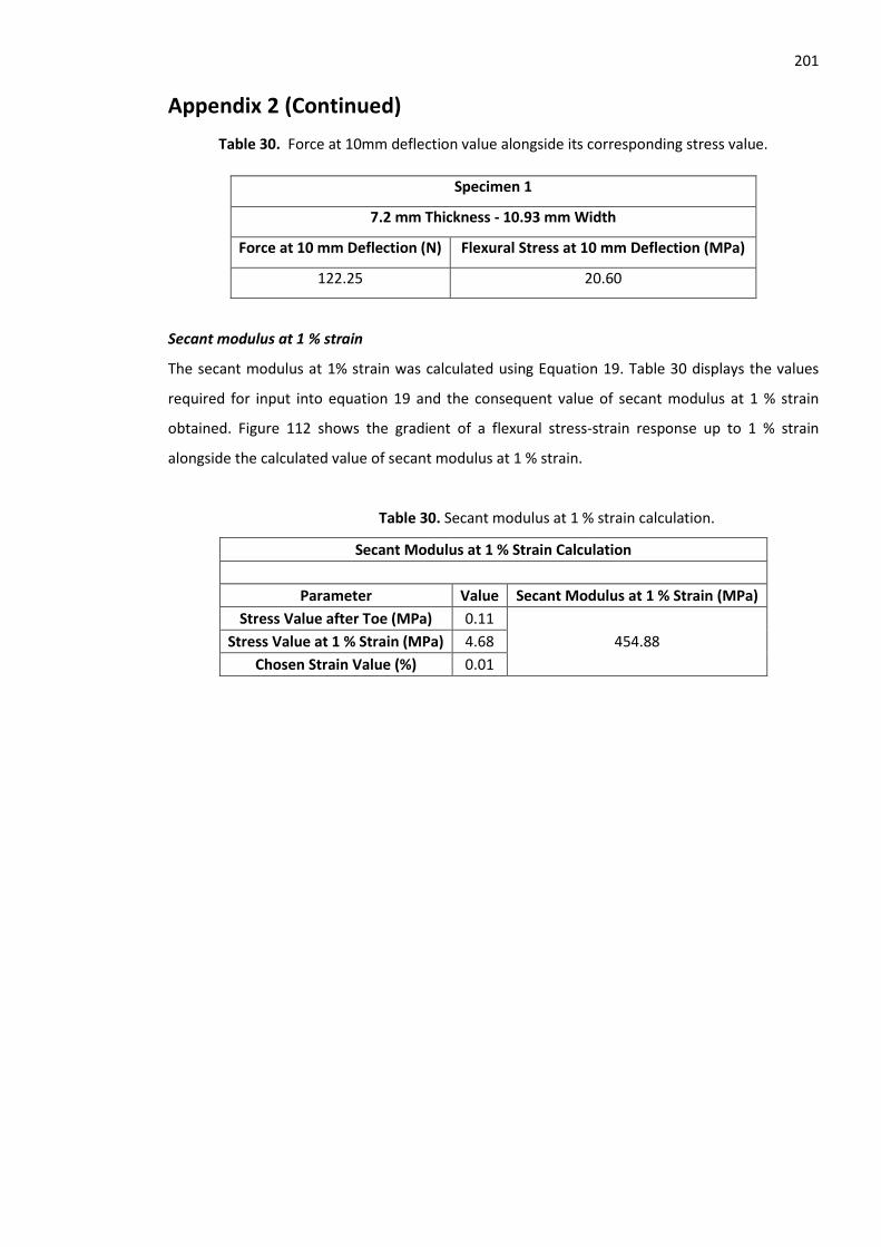
201

Appendix 2 (Continued)

Table 30. Force at 10mm deflection value alongside its corresponding stress value.

Specimen 1

7.2 mm Thickness - 10.93 mm Width

Force at 10 mm Deflection (N) Flexural Stress at 10 mm Deflection (MPa)

122.25 20.60

Secant modulus at 1 % strain

The secant modulus at 1% strain was calculated using Equation 19. Table 30 displays the values

required for input into equation 19 and the consequent value of secant modulus at 1 % strain

obtained. Figure 112 shows the gradient of a flexural stress-strain response up to 1 % strain

alongside the calculated value of secant modulus at 1 % strain.

Table 30. Secant modulus at 1 % strain calculation.

Secant Modulus at 1 % Strain Calculation

Parameter Value Secant Modulus at 1 % Strain (MPa)

Stress Value after Toe (MPa) 0.11

454.88 Stress Value at 1 % Strain (MPa) 4.68

Chosen Strain Value (%) 0.01

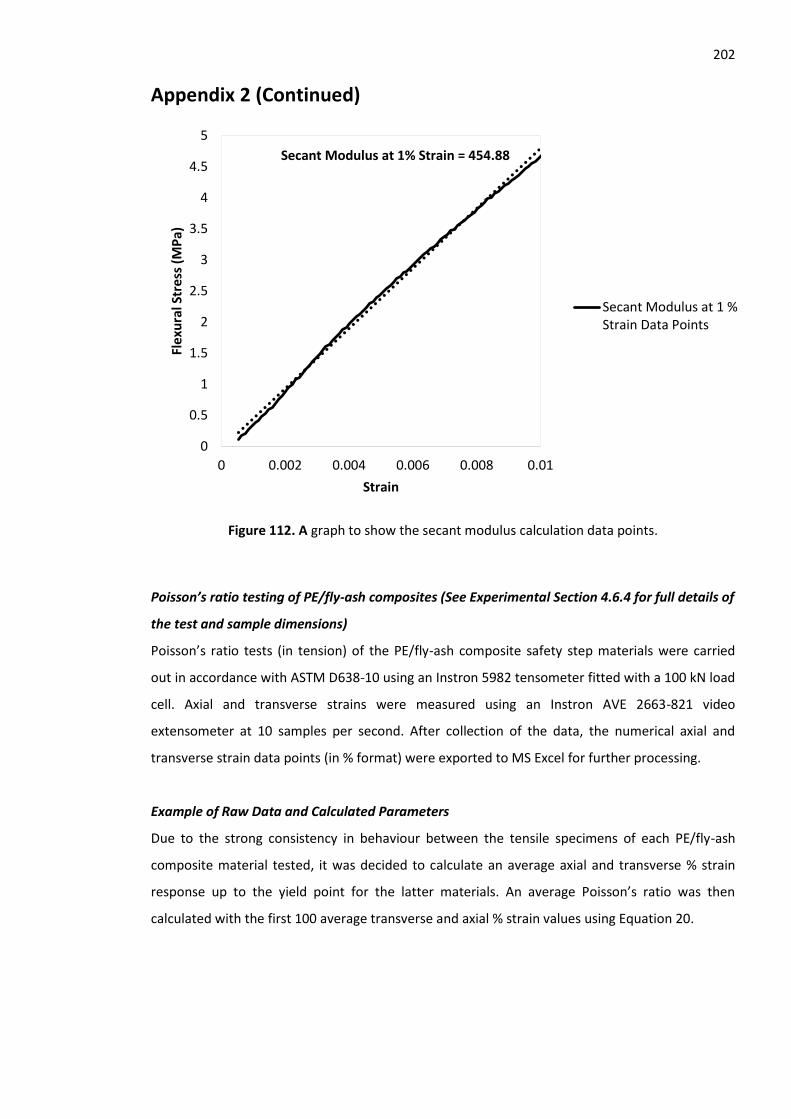
202

Appendix 2 (Continued)

Figure 112. A graph to show the secant modulus calculation data points.

Poisson’s ratio testing of PE/fly-ash composites (See Experimental Section 4.6.4 for full details of

the test and sample dimensions)

Poisson’s ratio tests (in tension) of the PE/fly-ash composite safety step materials were carried

out in accordance with ASTM D638-10 using an Instron 5982 tensometer fitted with a 100 kN load

cell. Axial and transverse strains were measured using an Instron AVE 2663-821 video

extensometer at 10 samples per second. After collection of the data, the numerical axial and

transverse strain data points (in % format) were exported to MS Excel for further processing.

Example of Raw Data and Calculated Parameters

Due to the strong consistency in behaviour between the tensile specimens of each PE/fly-ash

composite material tested, it was decided to calculate an average axial and transverse % strain

response up to the yield point for the latter materials. An average Poisson’s ratio was then

calculated with the first 100 average transverse and axial % strain values using Equation 20.

Secant Modulus at 1% Strain = 454.88

0

0.5

1

1.5

2

2.5

3

3.5

4

4.5

5

0 0.002 0.004 0.006 0.008 0.01

Fle

xura

l Str

ess

(MP

a)

Strain

Secant Modulus at 1 %Strain Data Points

203

Appendix 2 (Continued)

Standard deviations were also calculated. The latter effectively resulted in a value of Poisson’s

ratio close to or at the yield point, rather than within the elastic region (see Figure 15 in

Experimental Section 4.6.2). Table 31 shows how the raw data translated into Poisson’s ratio

values.

Table 31. Tensile test data and consequent calculation of Poisson’s ratio.

Time (s)

Average Load (N)

Average Video Axial Strain (%)

Average Video Transverse Strain (%)

Average Poissons Ratio

0 3.95 0.0485 0.0012 0.0251

0.1 4.55 0.0560 0.0007 0.0117

0.2 12.47 0.1535 0.0090 0.0588

0.3 17.75 0.2184 0.0228 0.1043

0.4 22.63 0.2786 0.0347 0.1247

0.5 27.22 0.3351 0.0434 0.1295

0.6 31.92 0.3930 0.0539 0.1371

0.7 36.71 0.4519 0.0599 0.1325

0.8 41.39 0.5095 0.0714 0.1402

0.9 45.78 0.5635 0.0806 0.1431

1 49.94 0.6148 0.0890 0.1448

Safety Step Compression Testing

Full details of the compression test equipment, methods and sample dimensions are provided in

Experimental Section 4.6.6 of this thesis for all safety steps. Both left and right sidewall

deflections during the tests were measured and averaged at 20 N intervals using two Mitutoyo

dial test indicators, standard deviation was also calculated; an example of this is in Table 32.

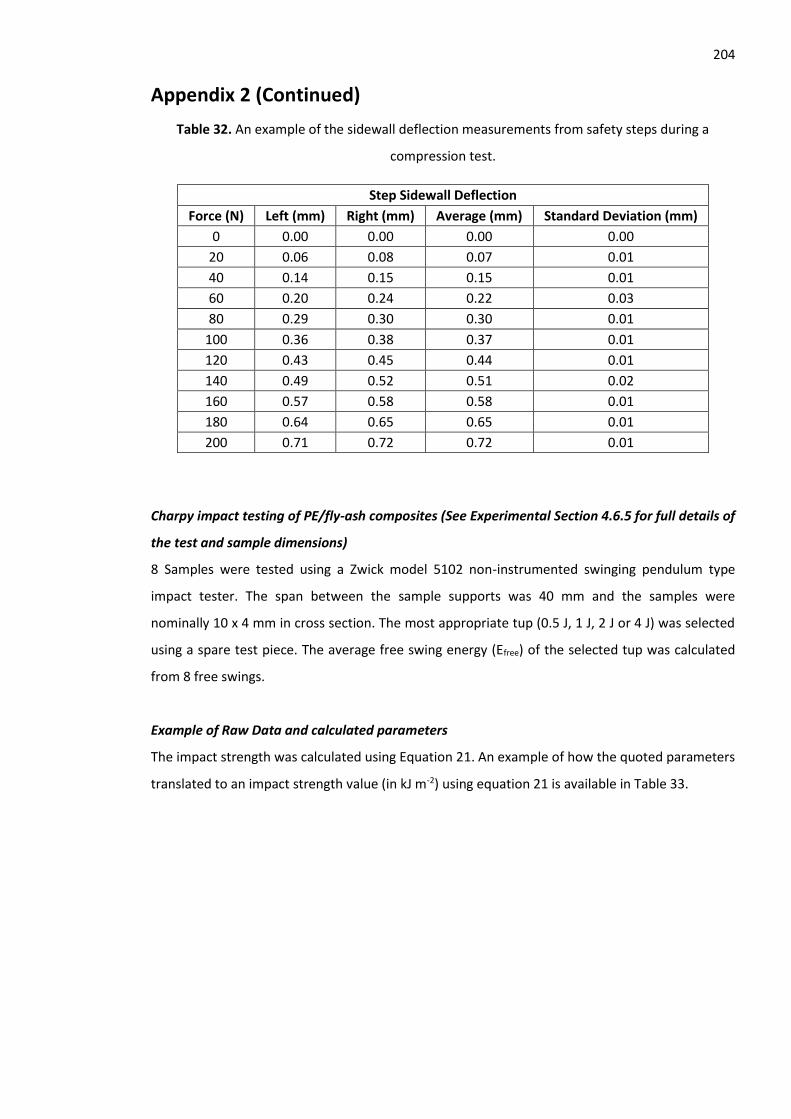
204

Appendix 2 (Continued)

Table 32. An example of the sidewall deflection measurements from safety steps during a

compression test.

Step Sidewall Deflection

Force (N) Left (mm) Right (mm) Average (mm) Standard Deviation (mm)

0 0.00 0.00 0.00 0.00

20 0.06 0.08 0.07 0.01

40 0.14 0.15 0.15 0.01

60 0.20 0.24 0.22 0.03

80 0.29 0.30 0.30 0.01

100 0.36 0.38 0.37 0.01

120 0.43 0.45 0.44 0.01

140 0.49 0.52 0.51 0.02

160 0.57 0.58 0.58 0.01

180 0.64 0.65 0.65 0.01

200 0.71 0.72 0.72 0.01

Charpy impact testing of PE/fly-ash composites (See Experimental Section 4.6.5 for full details of

the test and sample dimensions)

8 Samples were tested using a Zwick model 5102 non-instrumented swinging pendulum type

impact tester. The span between the sample supports was 40 mm and the samples were

nominally 10 x 4 mm in cross section. The most appropriate tup (0.5 J, 1 J, 2 J or 4 J) was selected

using a spare test piece. The average free swing energy (Efree) of the selected tup was calculated

from 8 free swings.

Example of Raw Data and calculated parameters

The impact strength was calculated using Equation 21. An example of how the quoted parameters

translated to an impact strength value (in kJ m-2) using equation 21 is available in Table 33.

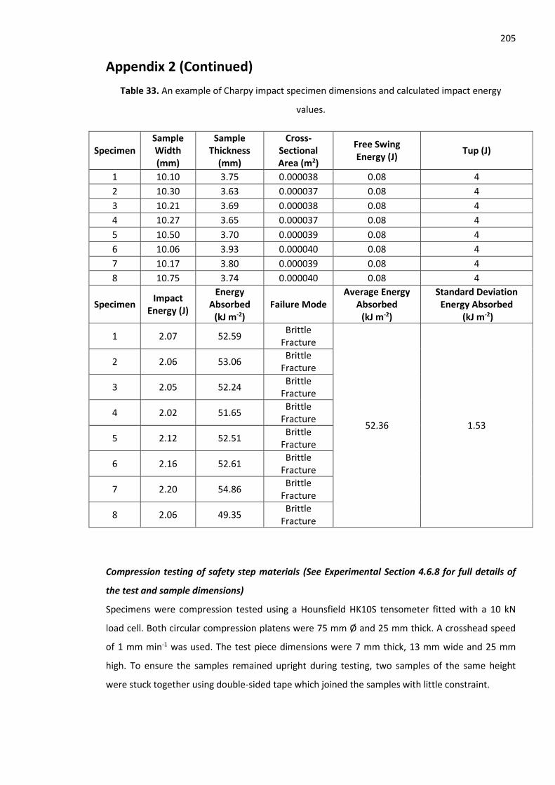
205

Appendix 2 (Continued)

Table 33. An example of Charpy impact specimen dimensions and calculated impact energy

values.

Specimen Sample Width (mm)

Sample Thickness

(mm)

Cross-Sectional Area (m2)

Free Swing Energy (J)

Tup (J)

1 10.10 3.75 0.000038 0.08 4

2 10.30 3.63 0.000037 0.08 4

3 10.21 3.69 0.000038 0.08 4

4 10.27 3.65 0.000037 0.08 4

5 10.50 3.70 0.000039 0.08 4

6 10.06 3.93 0.000040 0.08 4

7 10.17 3.80 0.000039 0.08 4

8 10.75 3.74 0.000040 0.08 4

Specimen Impact

Energy (J)

Energy Absorbed

(kJ m-2) Failure Mode

Average Energy Absorbed

(kJ m-2)

Standard Deviation Energy Absorbed

(kJ m-2)

1 2.07 52.59 Brittle

Fracture

52.36 1.53

2 2.06 53.06 Brittle

Fracture

3 2.05 52.24 Brittle

Fracture

4 2.02 51.65 Brittle

Fracture

5 2.12 52.51 Brittle

Fracture

6 2.16 52.61 Brittle

Fracture

7 2.20 54.86 Brittle

Fracture

8 2.06 49.35 Brittle

Fracture

Compression testing of safety step materials (See Experimental Section 4.6.8 for full details of

the test and sample dimensions)

Specimens were compression tested using a Hounsfield HK10S tensometer fitted with a 10 kN

load cell. Both circular compression platens were 75 mm Ø and 25 mm thick. A crosshead speed

of 1 mm min-1 was used. The test piece dimensions were 7 mm thick, 13 mm wide and 25 mm

high. To ensure the samples remained upright during testing, two samples of the same height

were stuck together using double-sided tape which joined the samples with little constraint.

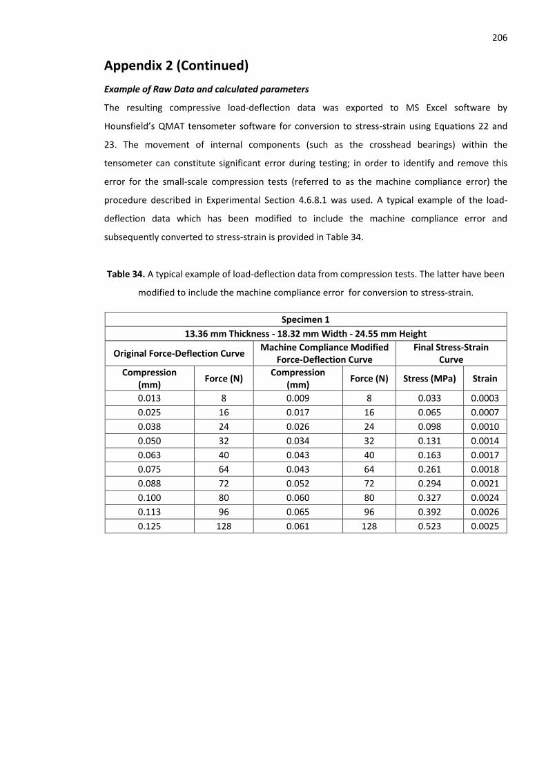
206

Appendix 2 (Continued)

Example of Raw Data and calculated parameters

The resulting compressive load-deflection data was exported to MS Excel software by

Hounsfield’s QMAT tensometer software for conversion to stress-strain using Equations 22 and

23. The movement of internal components (such as the crosshead bearings) within the

tensometer can constitute significant error during testing; in order to identify and remove this

error for the small-scale compression tests (referred to as the machine compliance error) the

procedure described in Experimental Section 4.6.8.1 was used. A typical example of the load-

deflection data which has been modified to include the machine compliance error and

subsequently converted to stress-strain is provided in Table 34.

Table 34. A typical example of load-deflection data from compression tests. The latter have been

modified to include the machine compliance error for conversion to stress-strain.

Specimen 1

13.36 mm Thickness - 18.32 mm Width - 24.55 mm Height

Original Force-Deflection Curve Machine Compliance Modified

Force-Deflection Curve Final Stress-Strain

Curve

Compression (mm)

Force (N) Compression

(mm) Force (N) Stress (MPa) Strain

0.013 8 0.009 8 0.033 0.0003

0.025 16 0.017 16 0.065 0.0007

0.038 24 0.026 24 0.098 0.0010

0.050 32 0.034 32 0.131 0.0014

0.063 40 0.043 40 0.163 0.0017

0.075 64 0.043 64 0.261 0.0018

0.088 72 0.052 72 0.294 0.0021

0.100 80 0.060 80 0.327 0.0024

0.113 96 0.065 96 0.392 0.0026

0.125 128 0.061 128 0.523 0.0025

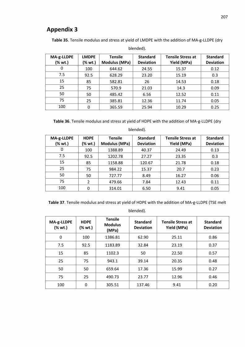
207

Appendix 3

Table 35. Tensile modulus and stress at yield of LMDPE with the addition of MA-g-LLDPE (dry

blended).

MA-g-LLDPE (% wt.)

LMDPE (% wt.)

Tensile Modulus (MPa)

Standard Deviation

Tensile Stress at Yield (MPa)

Standard Deviation

0 100 644.62 24.55 15.37 0.12

7.5 92.5 628.29 23.20 15.19 0.3

15 85 582.81 26 14.53 0.18

25 75 570.9 21.03 14.3 0.09

50 50 485.42 6.56 12.52 0.11

75 25 385.81 12.36 11.74 0.05

100 0 365.59 25.94 10.29 0.25

Table 36. Tensile modulus and stress at yield of HDPE with the addition of MA-g-LLDPE (dry

blended).

MA-g-LLDPE (% wt.)

HDPE (% wt.)

Tensile Modulus (MPa)

Standard Deviation

Tensile Stress at Yield (MPa)

Standard Deviation

0 100 1388.89 40.37 24.49 0.13

7.5 92.5 1202.78 27.27 23.35 0.3

15 85 1158.88 120.67 21.78 0.18

25 75 984.22 15.37 20.7 0.23

50 50 727.77 8.49 16.27 0.06

75 2 479.66 7.84 12.43 0.11

100 0 314.01 6.50 9.41 0.05

Table 37. Tensile modulus and stress at yield of HDPE with the addition of MA-g-LLDPE (TSE melt

blended).

MA-g-LLDPE (% wt.)

HDPE (% wt.)

Tensile Modulus

(MPa)

Standard Deviation

Tensile Stress at Yield (MPa)

Standard Deviation

0 100 1386.81 62.90 25.11 0.86

7.5 92.5 1183.89 32.84 23.19 0.37

15 85 1102.3 50 22.50 0.57

25 75 943.1 39.14 20.35 0.48

50 50 659.64 17.36 15.99 0.27

75 25 490.73 23.77 12.96 0.46

100 0 305.51 137.46 9.41 0.20

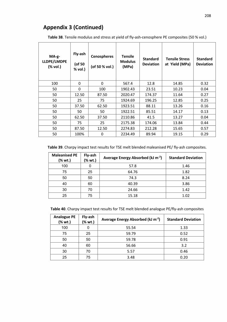
208

Appendix 3 (Continued)

Table 38. Tensile modulus and stress at yield of fly-ash-cenosphere PE composites (50 % vol.)

MA-g-LLDPE/LMDPE

(% vol.)

Fly-ash

(of 50 % vol.)

Cenospheres

(of 50 % vol.)

Tensile Modulus

(MPa)

Standard Deviation

Tensile Stress at Yield (MPa)

Standard Deviation

100 0 0 567.4 12.8 14.85 0.32

50 0 100 1902.43 23.51 10.23 0.04

50 12.50 87.50 2020.47 174.37 11.64 0.27

50 25 75 1924.69 196.25 12.85 0.25

50 37.50 62.50 1923.51 88.11 13.26 0.16

50 50 50 1922.51 85.51 14.17 0.13

50 62.50 37.50 2110.86 41.5 13.27 0.04

50 75 25 2175.38 174.06 13.84 0.44

50 87.50 12.50 2274.83 212.28 15.65 0.57

50 100% 0 2234.49 89.94 19.15 0.29

Table 39. Charpy impact test results for TSE melt blended maleanised PE/ fly-ash composites.

Maleanised PE (% wt.)

Fly-ash (% wt.)

Average Energy Absorbed (kJ m-2) Standard Deviation

100 0 57.8 1.46

75 25 64.76 1.82

50 50 74.3 8.24

40 60 40.39 3.86

30 70 24.66 1.42

25 75 15.18 1.02

Table 40. Charpy impact test results for TSE melt blended analogue PE/fly-ash composites

Analogue PE (% wt.)

Fly-ash (% wt.)

Average Energy Absorbed (kJ m-2) Standard Deviation

100 0 55.54 1.33

75 25 59.79 0.52

50 50 59.78 0.91

40 60 56.66 3.2

30 70 5.57 0.46

25 75 3.48 0.20

209

Appendix 4

Differential scanning calorimetry (See Experimental Section 4.9 for full details of the analysis

procedure)

DSC was carried out on the particulate-filled PE and unfilled PE materials. Sample mass was

typically between 4 and 10 mg. The crystalline content of unfilled PE materials was determined

using Equation 26. For PE/filler composites, crystallinity content was also calculated using

Equation 25. However, Equation 26 was used to calculate 𝛥Hf for input into Equation 25. The

following heat – hold – cool – heat cycle was used:

Heat from 20 °C to 240 °C at 20 °C min-1

Hold at 240 °C for 5 minutes

Cool from 240 °C to 20 oC at 20 °C min-1

Hold at 20 °C for 2 minutes

Heat from 20 °C to 240 °C at 20 °C min-1

Samples were heated in a nitrogen atmosphere (flow rate 30 cm3 min-1). The following

parameters were recorded during DSC:

1st Heat

Onset of melting temperature

Peak melting temperature

Melting temperature range

Heat of fusion 𝛥Hf (for calculation of crystalline content. The samples were held at 240 oC

for five minutes to ensure complete melting and total eradication of previous thermal

history)

Cool from melt

Onset of crystallisation temperature

Crystallisation exotherm peak temperature

Crystallisation temperature range

Heat of crystallisation (for calculation of crystalline content obtained during controlled

crystallisation)

2nd Heat

The same parameters as recorded during the 1st heat were recorded

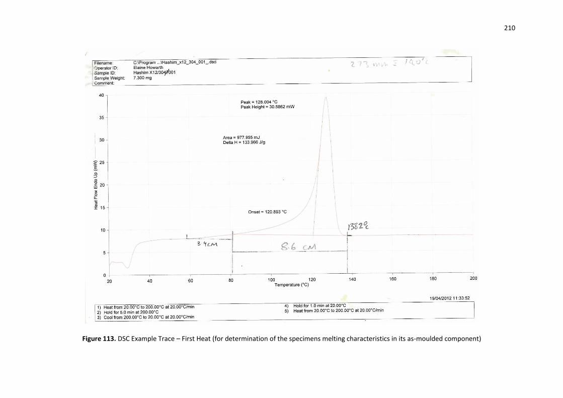
210

Figure 113. DSC Example Trace – First Heat (for determination of the specimens melting characteristics in its as-moulded component)

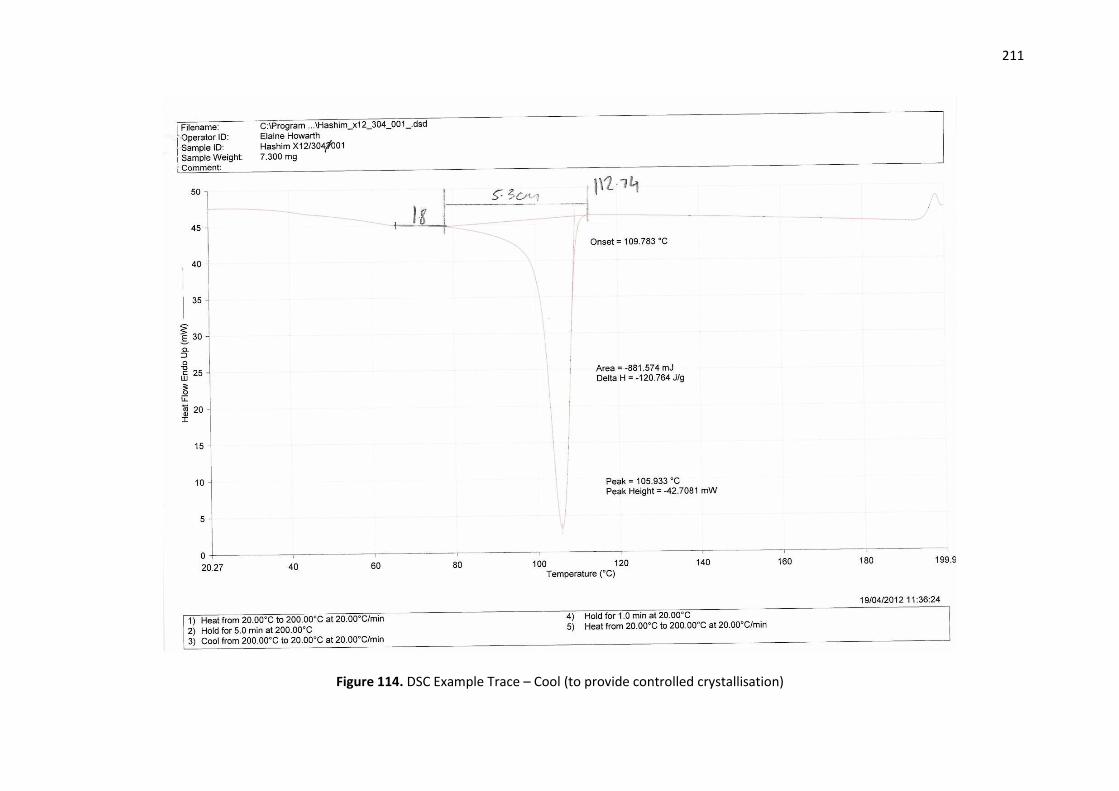
211

Figure 114. DSC Example Trace – Cool (to provide controlled crystallisation)

212

Figure 115. DSC Example Trace – Second Heat (to examine the melting of crystal structures formed because of controlled crystallisation)

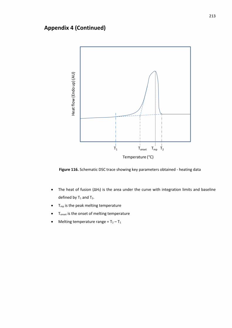
213

Appendix 4 (Continued)

Figure 116. Schematic DSC trace showing key parameters obtained - heating data

The heat of fusion (∆Hf) is the area under the curve with integration limits and baseline

defined by T1 and T2.

Tmp is the peak melting temperature

Tonset is the onset of melting temperature

Melting temperature range = T2 – T1

TmpTonset T2T1

Temperature (°C)

He

at f

low

(En

do

up

) (A

U)

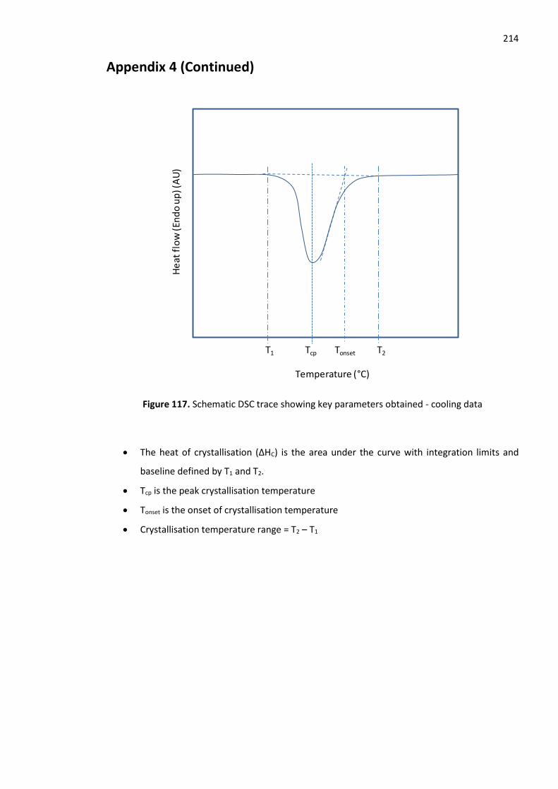
214

Appendix 4 (Continued)

Figure 117. Schematic DSC trace showing key parameters obtained - cooling data

The heat of crystallisation (∆HC) is the area under the curve with integration limits and

baseline defined by T1 and T2.

Tcp is the peak crystallisation temperature

Tonset is the onset of crystallisation temperature

Crystallisation temperature range = T2 – T1

Tcp Tonset T2T1

Temperature (°C)

He

at f

low

(En

do

up

) (A

U)

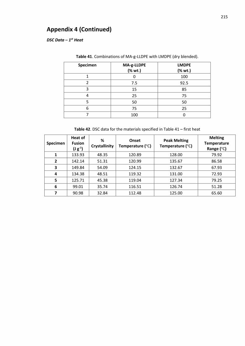
215

Appendix 4 (Continued)

DSC Data – 1st Heat

Table 41. Combinations of MA-g-LLDPE with LMDPE (dry blended).

Specimen MA-g-LLDPE (% wt.)

LMDPE (% wt.)

1 0 100

2 7.5 92.5

3 15 85

4 25 75

5 50 50

6 75 25

7 100 0

Table 42. DSC data for the materials specified in Table 41 – first heat

Specimen Heat of Fusion (J g-1)

% Crystallinity

Onset Temperature (oC)

Peak Melting Temperature (oC)

Melting Temperature

Range (oC)

1 133.93 48.35 120.89 128.00 79.92

2 142.14 51.31 120.99 135.67 86.58

3 149.84 54.09 124.15 132.67 67.93

4 134.38 48.51 119.32 131.00 72.93

5 125.71 45.38 119.04 127.34 79.25

6 99.01 35.74 116.51 126.74 51.28

7 90.98 32.84 112.48 125.00 65.60

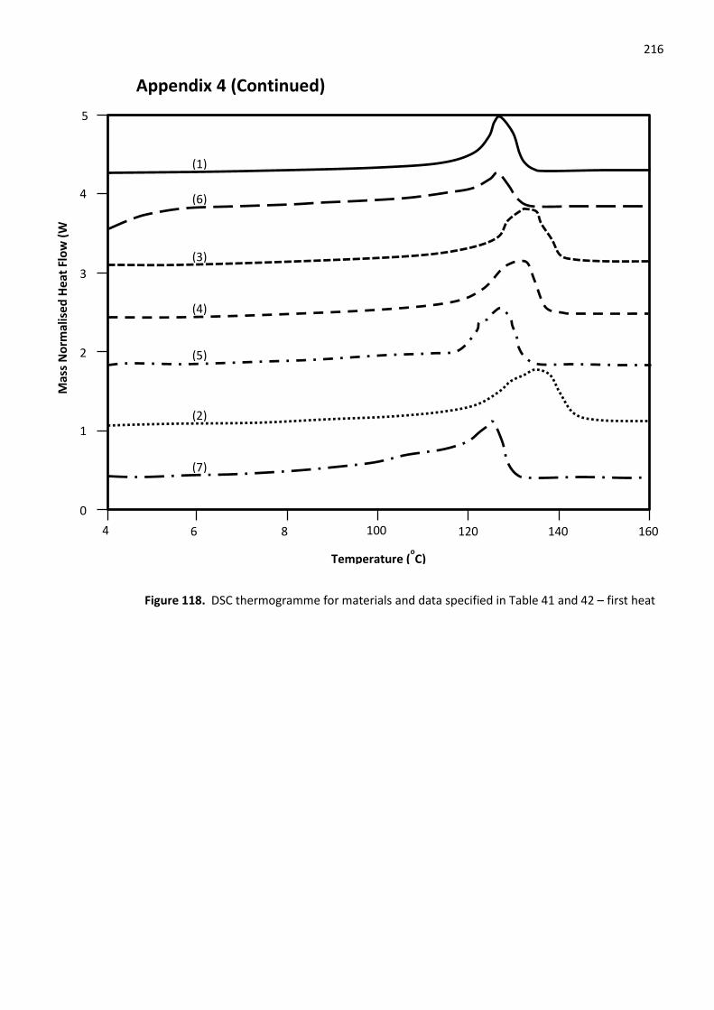
216

Appendix 4 (Continued)

Figure 118. DSC thermogramme for materials and data specified in Table 41 and 42 – first heat

60

160 80

140 120

5

0

4

3

2

40

Temperature (oC)

Mas

s N

orm

alis

ed H

eat

Flo

w (

W

g-1)

100

1

(4)

(3)

(6)

(1)

(5)

(2)

(7)

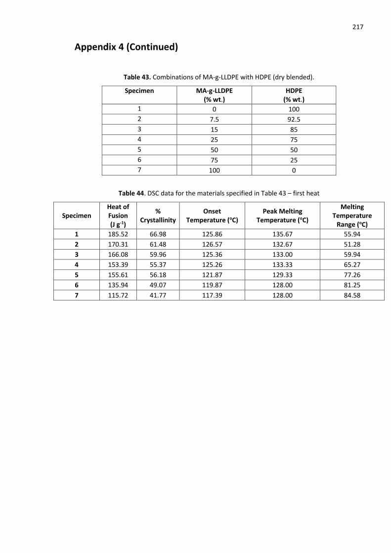
217

Appendix 4 (Continued)

Table 43. Combinations of MA-g-LLDPE with HDPE (dry blended).

Specimen MA-g-LLDPE (% wt.)

HDPE (% wt.)

1 0 100

2 7.5 92.5

3 15 85

4 25 75

5 50 50

6 75 25

7 100 0

Table 44. DSC data for the materials specified in Table 43 – first heat

Specimen Heat of Fusion (J g-1)

% Crystallinity

Onset Temperature (oC)

Peak Melting Temperature (oC)

Melting Temperature

Range (oC)

1 185.52 66.98 125.86 135.67 55.94

2 170.31 61.48 126.57 132.67 51.28

3 166.08 59.96 125.36 133.00 59.94

4 153.39 55.37 125.26 133.33 65.27

5 155.61 56.18 121.87 129.33 77.26

6 135.94 49.07 119.87 128.00 81.25

7 115.72 41.77 117.39 128.00 84.58

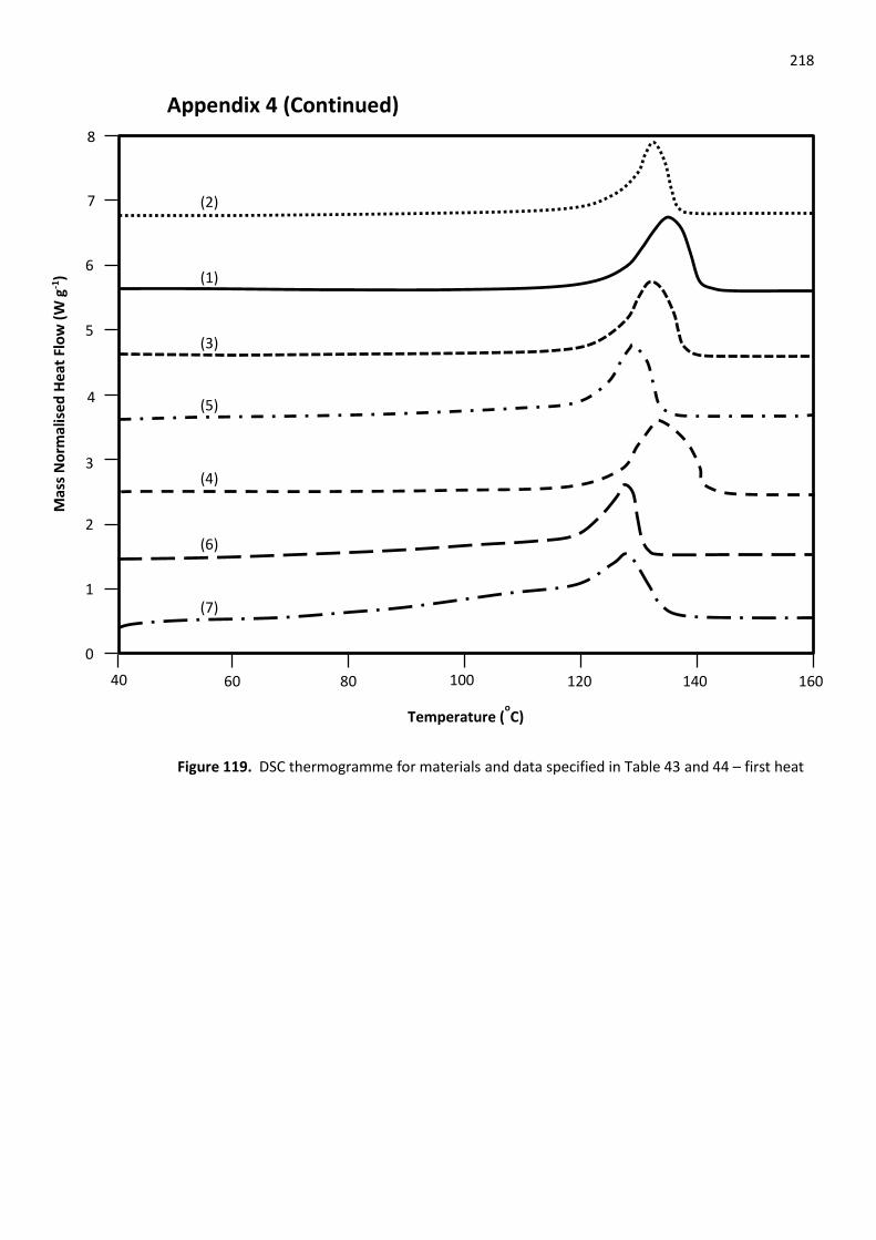
218

Appendix 4 (Continued)

Figure 119. DSC thermogramme for materials and data specified in Table 43 and 44 – first heat

60 160 80 140 120

8

0

6

1

5

2

3

40

Temperature (oC)

Mas

s N

orm

alis

ed H

eat

Flo

w (

W g

-1)

100

(4)

(6)

(7)

(5)

(3)

(1)

(2)

4

7

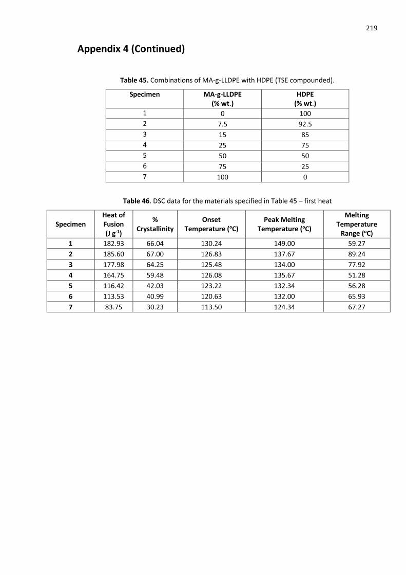
219

Appendix 4 (Continued)

Table 45. Combinations of MA-g-LLDPE with HDPE (TSE compounded).

Specimen MA-g-LLDPE (% wt.)

HDPE (% wt.)

1 0 100

2 7.5 92.5

3 15 85

4 25 75

5 50 50

6 75 25

7 100 0

Table 46. DSC data for the materials specified in Table 45 – first heat

Specimen Heat of Fusion (J g-1)

% Crystallinity

Onset Temperature (oC)

Peak Melting Temperature (oC)

Melting Temperature

Range (oC)

1 182.93 66.04 130.24 149.00 59.27

2 185.60 67.00 126.83 137.67 89.24

3 177.98 64.25 125.48 134.00 77.92

4 164.75 59.48 126.08 135.67 51.28

5 116.42 42.03 123.22 132.34 56.28

6 113.53 40.99 120.63 132.00 65.93

7 83.75 30.23 113.50 124.34 67.27

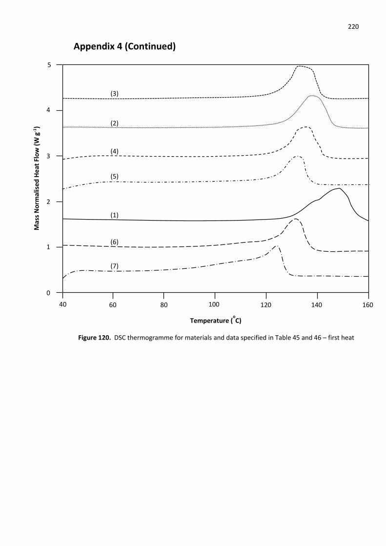
220

Appendix 4 (Continued)

Figure 120. DSC thermogramme for materials and data specified in Table 45 and 46 – first heat

60 160 80 140 120

5

0

4

3

2

40

Temperature (oC)

Mas

s N

orm

alis

ed H

eat

Flo

w (

W g

-1)

100

(5)

(4)

(2)

(3)

(1)

(6)

(7)

1

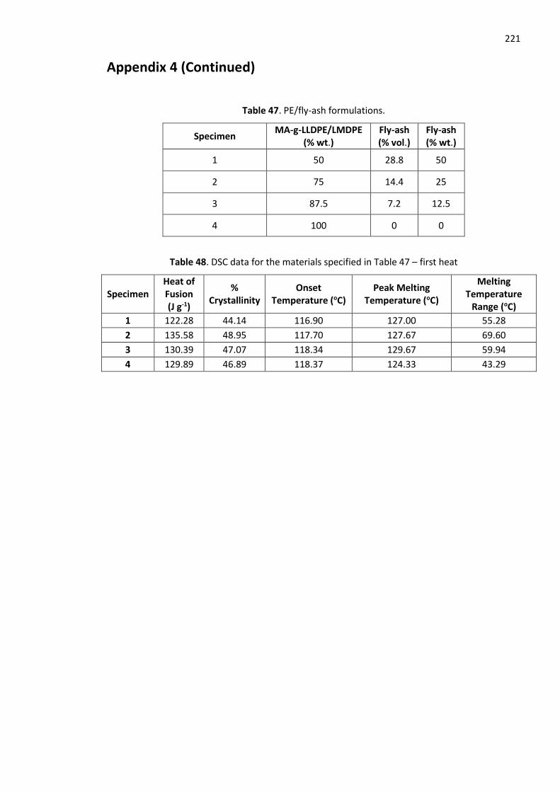
221

Appendix 4 (Continued)

Table 47. PE/fly-ash formulations.

Specimen MA-g-LLDPE/LMDPE

(% wt.) Fly-ash (% vol.)

Fly-ash (% wt.)

1 50 28.8 50

2 75 14.4 25

3 87.5 7.2 12.5

4 100 0 0

Table 48. DSC data for the materials specified in Table 47 – first heat

Specimen Heat of Fusion (J g-1)

% Crystallinity

Onset Temperature (oC)

Peak Melting Temperature (oC)

Melting Temperature

Range (oC)

1 122.28 44.14 116.90 127.00 55.28

2 135.58 48.95 117.70 127.67 69.60

3 130.39 47.07 118.34 129.67 59.94

4 129.89 46.89 118.37 124.33 43.29

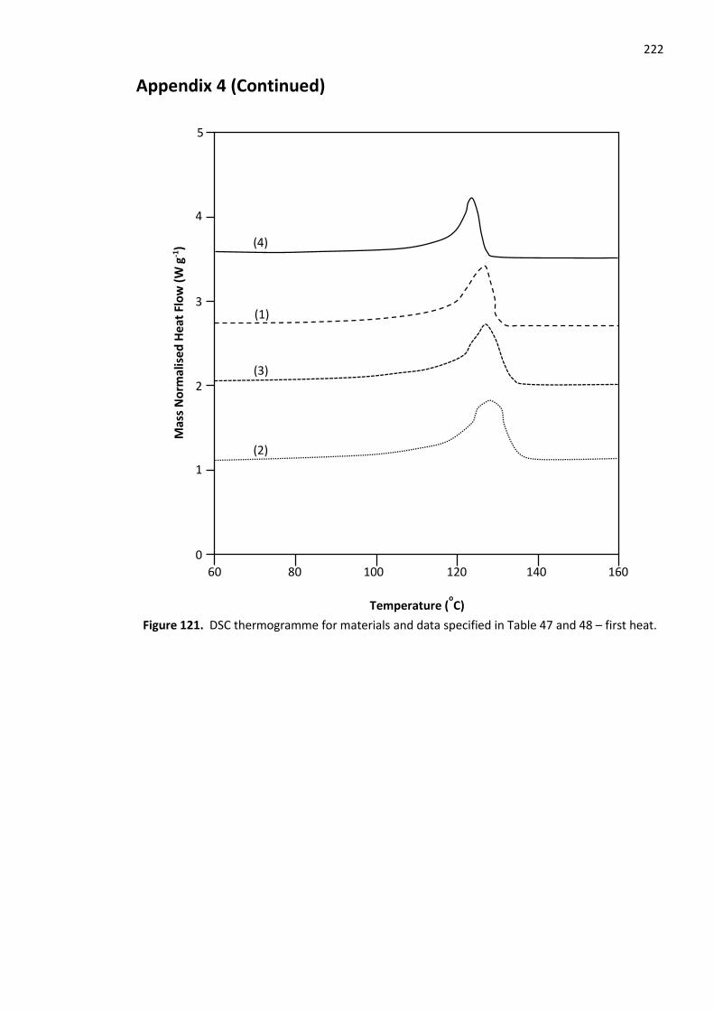
222

Appendix 4 (Continued)

Figure 121. DSC thermogramme for materials and data specified in Table 47 and 48 – first heat.

3

Temperature (oC)

80 160 140

5

0

4

2

Mas

s N

orm

alis

ed H

eat

Flo

w (

W g

-1)

120

1

60 100

(4)

(1)

(3)

(2)

223

Appendix 4 (Continued)

DSC Data – Cool from Melt

Table 49. DSC data for the materials specified in Table 41 – cool from melt

Specimen

Heat of

Crystallisation

(J g-1)

%

Crystallinity

Onset

Crystallisation

Temperature

(oC)

Crystallisation

Exotherm Peak

Temperature (oC)

Crystallisation

Temperature

Range (oC)

1 127.59 46.06 109.78 105.93 47.29

2 130.45 47.09 110.45 104.93 52.61

3 136.57 49.30 110.84 107.60 51.28

4 120.64 43.55 110.69 107.60 54.61

5 113.68 41.04 109.64 106.27 57.94

6 98.51 35.56 107.82 104.60 56.28

7 77.59 28.01 106.08 102.93 49.62

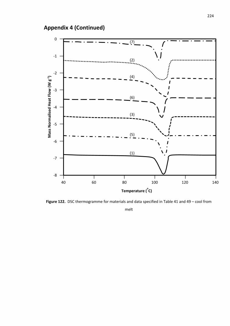
224

Appendix 4 (Continued)

Figure 122. DSC thermogramme for materials and data specified in Table 41 and 49 – cool from

melt

Mas

s N

orm

alis

ed H

eat

Flo

w (

W g

-1)

Temperature (oC)

40 140 60 80 120 100

0

-1

-8

-2

-3

-7

-4

-6

-5

(3)

(5)

(1)

(6)

(4)

(2)

(7)

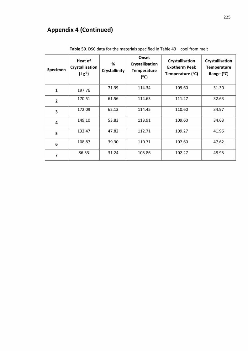
225

Appendix 4 (Continued)

Table 50. DSC data for the materials specified in Table 43 – cool from melt

Specimen

Heat of

Crystallisation

(J g-1)

%

Crystallinity

Onset

Crystallisation

Temperature

(oC)

Crystallisation

Exotherm Peak

Temperature (oC)

Crystallisation

Temperature

Range (oC)

1 197.76 71.39 114.34 109.60 31.30

2 170.51 61.56 114.63 111.27 32.63

3 172.09 62.13 114.45 110.60 34.97

4 149.10 53.83 113.91 109.60 34.63

5 132.47 47.82 112.71 109.27 41.96

6 108.87 39.30 110.71 107.60 47.62

7 86.53 31.24 105.86 102.27 48.95

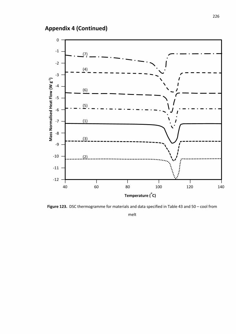
226

Appendix 4 (Continued)

Figure 123. DSC thermogramme for materials and data specified in Table 43 and 50 – cool from

melt

Mas

s N

orm

alis

ed H

eat

Flo

w (

W g

-1)

Temperature (oC)

40 140 60 80 120 100

0

-2

-12

-3

-5

-10

-6

-8

-9

-1

-11

-4

-7 (1)

(3)

(2)

(5)

(6)

(4)

(7)

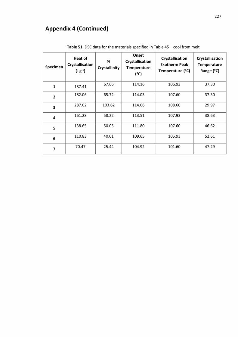
227

Appendix 4 (Continued)

Table 51. DSC data for the materials specified in Table 45 – cool from melt

Specimen

Heat of

Crystallisation

(J g-1)

%

Crystallinity

Onset

Crystallisation

Temperature

(oC)

Crystallisation

Exotherm Peak

Temperature (oC)

Crystallisation

Temperature

Range (oC)

1 187.41 67.66 114.16 106.93 37.30

2 182.06 65.72 114.03 107.60 37.30

3 287.02 103.62 114.06 108.60 29.97

4 161.28 58.22 113.51 107.93 38.63

5 138.65 50.05 111.80 107.60 46.62

6 110.83 40.01 109.65 105.93 52.61

7 70.47 25.44 104.92 101.60 47.29

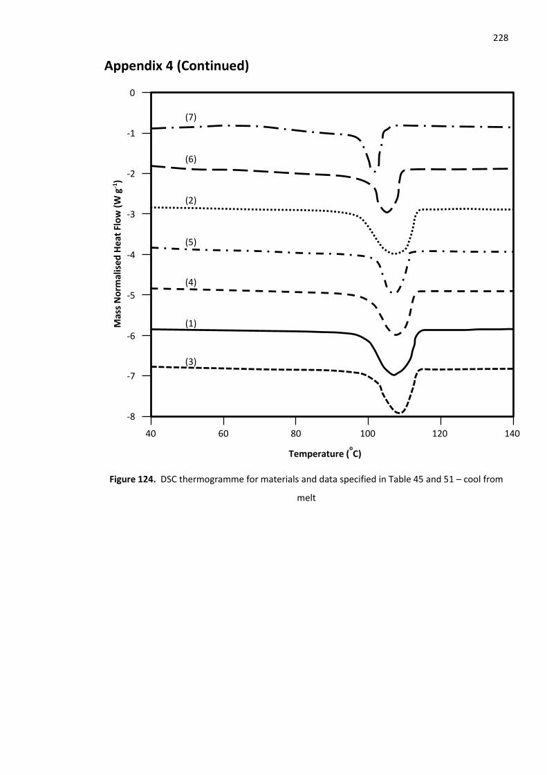
228

Appendix 4 (Continued)

Figure 124. DSC thermogramme for materials and data specified in Table 45 and 51 – cool from

melt

Mas

s N

orm

alis

ed H

eat

Flo

w (

W g

-1)

Temperature (oC)

40 140 60 80 120 100

0

-1

-8

-2

-3

-7

-4

-6

-5

(4)

(1)

(3)

(5)

(2)

(6)

(7)

229

Appendix 4 (Continued)

Table 52. DSC data for the materials specified in Table 47 – cool from melt

Specimen

Heat of

Crystallisation

(J g-1)

%

Crystallinity

Onset

Crystallisation

Temperature (oC)

Crystallisation

Exotherm Peak

Temperature (oC)

Crystallisation

Temperature

Range (oC)

1 124.98 45.12 109.06 106.27 39.29

2 116.81 42.17 108.90 104.60 34.63

3 181.94 65.68 109.68 104.27 61.94

4 216.06 78.00 111.61 108.60 65.93

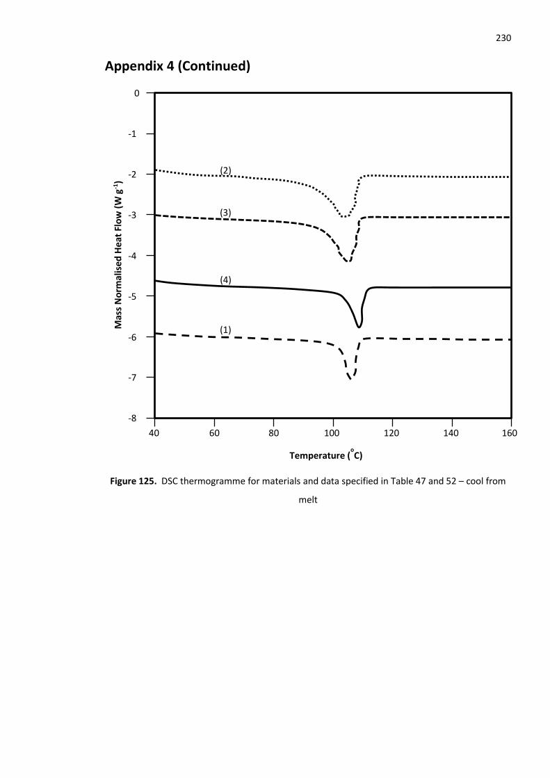
230

Appendix 4 (Continued)

Figure 125. DSC thermogramme for materials and data specified in Table 47 and 52 – cool from

melt

Mas

s N

orm

alis

ed H

eat

Flo

w (

W g

-1)

Temperature (oC)

40 140 80 120 100

0

-1

-8

-2

-3

-7

-4

-6

-5

(2)

(3)

(4)

(1)

60 160

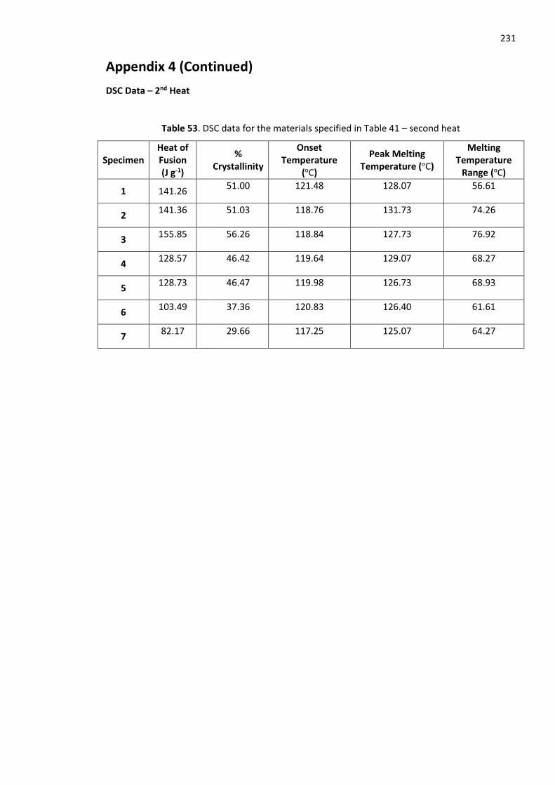
231

Appendix 4 (Continued)

DSC Data – 2nd Heat

Table 53. DSC data for the materials specified in Table 41 – second heat

Specimen Heat of Fusion (J g-1)

%

Crystallinity

Onset Temperature

(oC)

Peak Melting Temperature (oC)

Melting Temperature

Range (oC)

1 141.26 51.00 121.48 128.07 56.61

2 141.36 51.03 118.76 131.73 74.26

3 155.85 56.26 118.84 127.73 76.92

4 128.57 46.42 119.64 129.07 68.27

5 128.73 46.47 119.98 126.73 68.93

6 103.49 37.36 120.83 126.40 61.61

7 82.17 29.66 117.25 125.07 64.27

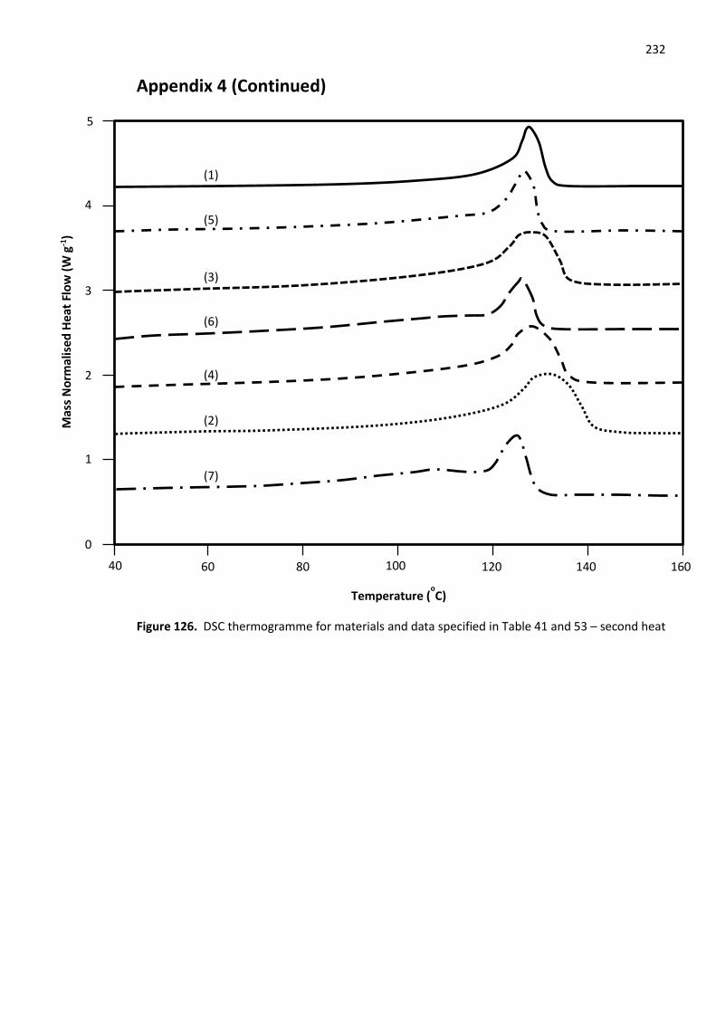
232

Appendix 4 (Continued)

Figure 126. DSC thermogramme for materials and data specified in Table 41 and 53 – second heat

60 160 80 140 120

5

0

4

3

2

40

Temperature (oC)

Mas

s N

orm

alis

ed H

eat

Flo

w (

W g

-1)

100

1

(6)

(3)

(5)

(1)

(4)

(2)

(7)

233

Appendix 4 (Continued)

Table 54. DSC data for the materials specified in Table 43 – second heat

Specimen Heat of Fusion (J g-1)

% Crystallinity

Onset Temperature (oC)

Peak Melting Temperature (oC)

Melting Temperature

Range (oC)

1 202.65 73.16 126.66 136.73 59.94

2 187.88 67.83 125.95 133.07 52.28

3 190.91 68.92 125.60 134.40 71.60

4 170.53 61.56 123.82 134.40 78.59

5 159.79 57.69 123.48 130.07 77.26

6 131.33 47.41 121.69 127.73 74.59

7 114.25 41.25 114.95 126.40 81.92

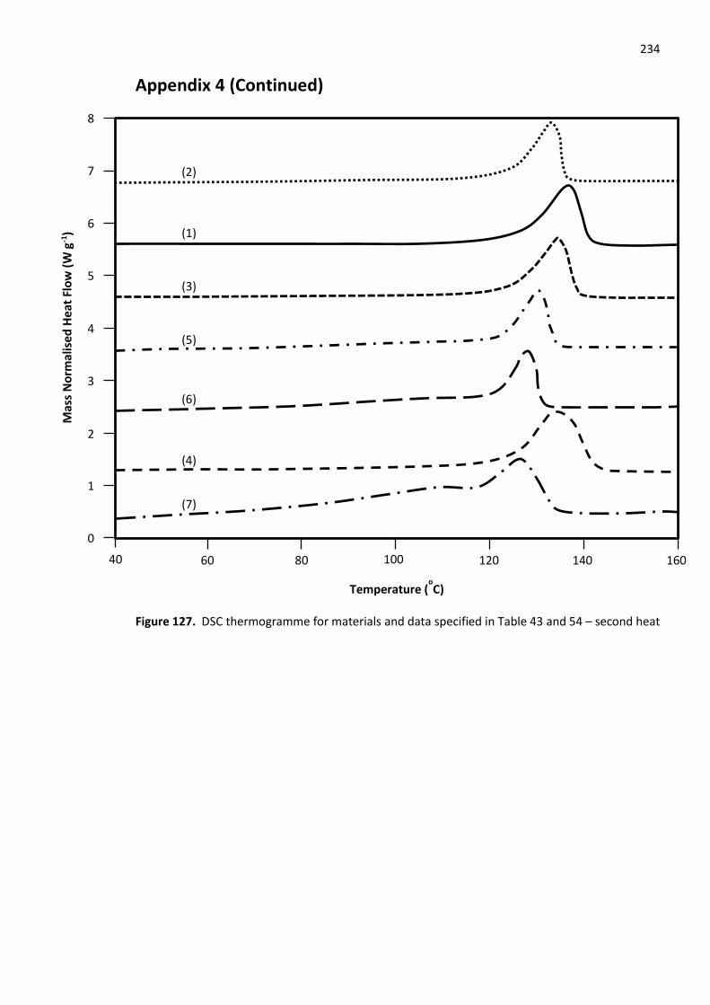
234

Appendix 4 (Continued)

Figure 127. DSC thermogramme for materials and data specified in Table 43 and 54 – second heat

60 160 80 140 120

8

7

0

6

5

1

4

2

3

40

Temperature (oC)

Mas

s N

orm

alis

ed H

eat

Flo

w (

W g

-1)

100

(6)

(4)

(7)

(5)

(3)

(1)

(2)

235

Appendix 4 (Continued)

Table 55. DSC data for the materials specified in Table 45 – second heat

Specimen Heat of Fusion (J g-1)

% Crystallinity

Onset Temperature (oC)

Peak Melting Temperature (oC)

Melting Temperature

Range (oC)

1 193.70 69.93 124.82 137.40 63.94

2 203.09 73.32 126.33 137.73 83.25

3 200.97 72.55 124.93 135.40 65.93

4 170.12 61.42 124.46 137.07 75.92

5 130.90 47.26 123.54 132.40 71.93

6 97.31 35.13 124.10 130.40 81.92

7 78.04 28.17 116.51 124.40 60.61

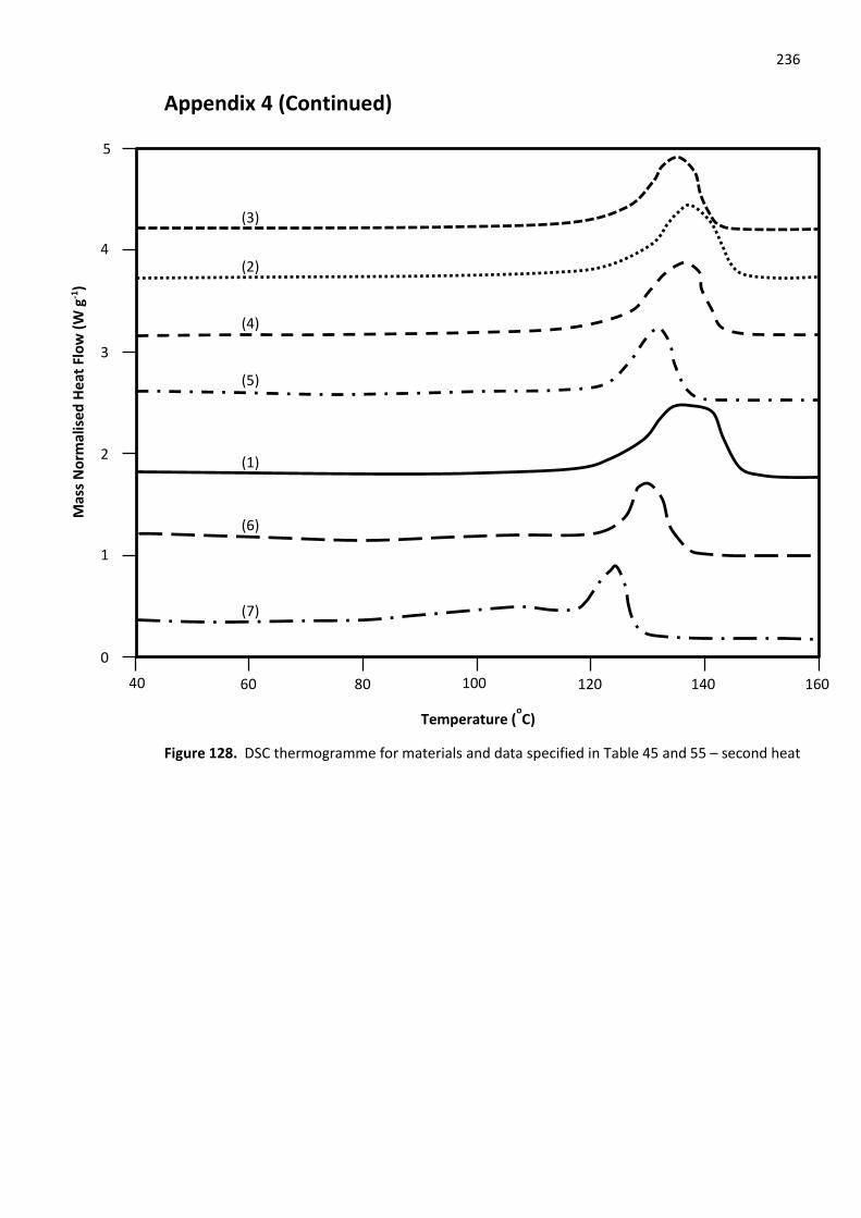
236

Appendix 4 (Continued)

Figure 128. DSC thermogramme for materials and data specified in Table 45 and 55 – second heat

(5)

(4)

(2)

(3)

(1)

(6)

(7)

60 160 80 140 120

5

0

4

3

2

40

Temperature (oC)

Mas

s N

orm

alis

ed H

eat

Flo

w (

W g

-1)

100

1

237

Appendix 4 (Continued)

Table 56. DSC data for the materials specified in Table 47 – second heat

Specimen Heat of Fusion (J g-1)

% Crystallinity

Onset Temperature (oC)

Peak Melting Temperature (oC)

Melting Temperature

Range (oC)

1 125.48 45.30 118.29 125.07 51.28

2 134.62 48.60 118.67 127.40 66.60

3 137.01 49.46 118.72 129.07 61.27

4 131.03 47.30 118.72 124.73 53.95

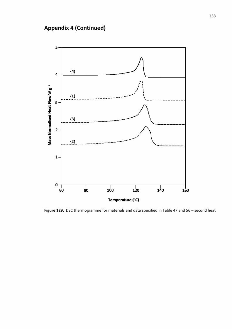
238

Appendix 4 (Continued)

Figure 129. DSC thermogramme for materials and data specified in Table 47 and 56 – second heat

239

Appendix 5

Data sheets of the polymers used in this PhD study.

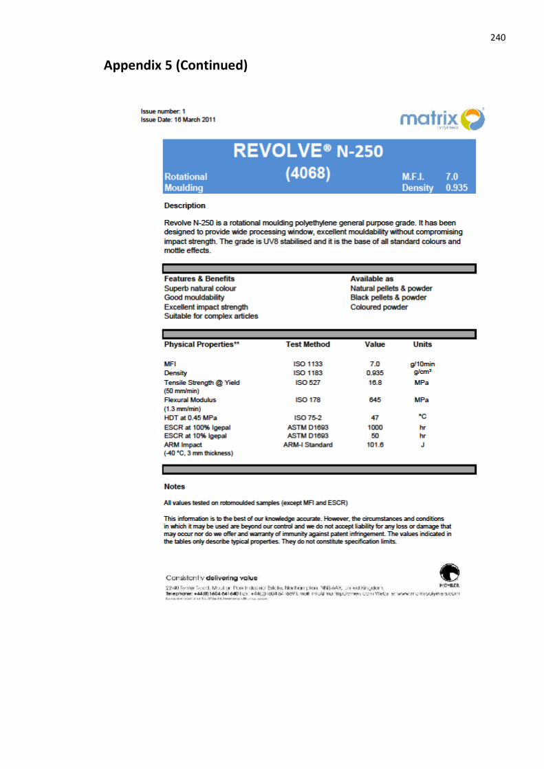
240

Appendix 5 (Continued)

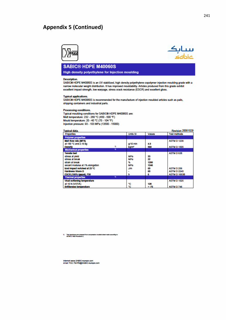
241

Appendix 5 (Continued)

242

Appendix 5 (Continued)

243

Appendix 5 (Continued)

244

Appendix 6

Data sheets of the filler particles used in this PhD study.

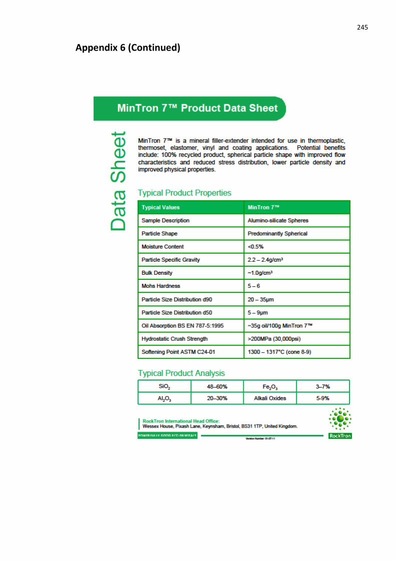
245

Appendix 6 (Continued)

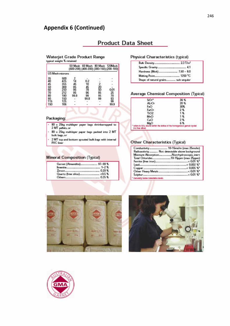
246

Appendix 6 (Continued)

247

Appendix 6 (Continued)