


Languages
Pages
Legal

University of Twente
Department of Computer Science
Software Engineering Group
A Metamodeling Approach to Incremental Model Changes
by
D.P.L. van der Meij
Master thesis
September 2008 to July 2009
Graduation committee:
dr. I. Kurtev (University of Twente), 1st supervisor
dr. ir. K.G. van den Berg (Univerity of Twente)
F. Wille (Novulo)

2
3
I ABSTRACT
For the next step in raising the level of abstraction in software development, Kent (Kent,
2002) proposed an approach for Model Driven Engineering (MDE). With MDE it is possible to raise the level of abstraction such that decisions can be made regardless the
implementation language. Business rules can be defined on a higher level so in fact programming happens at the level of models. Model transformations allow models to be turned into other models, for instance models of source code or other less abstract
models.
This thesis is about model‐to‐model and model‐to‐text transformations. Usually model‐to‐text aspects of thoughts are omitted because the text to be generated can also be modeled and thus a model‐to‐model transformation should be sufficient. Because in
this thesis we focus on incremental model changes and also incremental changing the files in the file system, we explicitly studied model‐to‐text transformation approaches to keep model and text synchronized. In this thesis we use different terms for model‐to‐
model and model‐to‐text transformations. We use the term transformation when we are dealing with models as logical entities, we use the term generation when we are dealing with files as physical entities. For instance, in a model‐to‐text transformation the
model will be transformed and the output will be generated files; the generation of files is due to the transformation of a model. We studied the possibilities to perform specific file generation and file modification based on a set of changes to a model.
In our approach we started investigating state of the art modeling environments and
concluded that they were not able to perform an incremental model place, with in‐place updates to a model. Also they did not support model‐to‐text transformations so for that reason we presented our own approach. The approach we propose in this thesis is an
imperative approach that is able to perform model‐to‐model and model‐to‐text transformations in parallel. We also present several implementations of our approach and benchmarked them against each other to see which implementation is the most
efficient when performing different types of (straightforward) transformations. Our results show that incremental model changes are indeed possible and also in an efficient way, optimized to the target platform.

4

5
II ABBREVIATIONS
Abbreviation Full description ANTLR ANother Tool for Language Recognition AST Abstract Syntax Tree ATL Atlas Transformation Language CIM Computational Independent Model CRM Customer Relationship Management DSL Domain Specific Language EBNF Extended Backus Naur Form EMF Eclipse Modeling Framework MDA Model Driven Architecture MDE Model Driven Engineering MOF Meta Object Facility OCL Object Constraint Language OMG Object Management Group OO Object Oriented PIM Platform Independent Model PHP Hypertext Preprocessor POC Proof of Concept PSM Platform Specific Model QVT Query / View / Transformation RFP Request for Proposal UML Unified Modeling Language VIATRA VIsual Automated TRAnsformations XML Extensible Markup Language

6

7
III LIST OF FIGURES
Figure 1: Thesis outline .................................................................................................... 21
Figure 2: MDA transformation, PIM to PSM [21]............................................................. 24
Figure 3: MOF metamodeling stack [22].......................................................................... 25
Figure 4: Comparison of the MOF stack to a program in C.............................................. 26
Figure 5: The basic model transformation pattern [18]................................................... 27
Figure 6: Relationships between QVT metamodels [23] ................................................. 28
Figure 7: Overview of ATL transformational approach [13] ............................................ 29
Figure 8: Re‐transformation [11] ..................................................................................... 30
Figure 9: Live transformation [11] ................................................................................... 31
Figure 10: Coarse‐grained transformation....................................................................... 32
Figure 11: Fine‐grained transformation........................................................................... 32
Figure 12: Transformation impact ................................................................................... 38
Figure 13: Venn diagram of delta .................................................................................... 39
Figure 14: Subset of delta that contains two additions ................................................... 40
Figure 15: Subset of delta that contains a change........................................................... 41
Figure 16: Subset of delta that contains a deletion ......................................................... 41
Figure 17: Example source model.................................................................................... 55
Figure 18: Delta with an addition .................................................................................... 55
Figure 19: Example resulting model after the transformation ........................................ 56
Figure 20: Metamodel for models in the computer’s memory ....................................... 61
Figure 21: Metamodel for entities in the file system....................................................... 62
Figure 22: Mapping of metamodels................................................................................. 63
8
Figure 23: Impact scale of model transformations .......................................................... 67
Figure 24: Entire model transformation map .................................................................. 67
Figure 25: Coarse‐grained model transformation map ................................................... 68
Figure 26: Fine‐grained model transformation map........................................................ 69
Figure 27: Screenshot of the Novulo Architect ................................................................ 73
Figure 28: Distribution of model revisions against number of nodes.............................. 75
Figure 29: Total distribution of timings of 1000 experiments ......................................... 80
Figure 30: Trimmed distribution of timings of 1000 experiments ................................... 81
Figure 31: Benchmarks 1 to 5: nr of pages vs. time ......................................................... 82
Figure 32: Benchmarks 6 to 10: nr of fields vs. time........................................................ 83
Figure 33: Benchmarks 11 to 15: nr of pages vs. time ..................................................... 84
Figure 34: Benchmarks 16 to 20: nr of fields vs. time...................................................... 85
Figure 35: Benchmarks 21 to 25: nr of pages vs. time ..................................................... 86
Figure 36: Benchmarks 26 to 30: nr of fields vs. time...................................................... 87
Figure 37: Class diagram of PoC....................................................................................... 99

9
IV LIST OF TABLES
Table 1: Properties of state of the art model transformation techniques....................... 50
Table 2: Additional mappings between metamodels ...................................................... 64
Table 3: Model‐to‐text approaches ................................................................................. 67
Table 4: Properties of entities in the file system ............................................................. 78
Table 5: Addition benchmarks ......................................................................................... 81
Table 6: Changes benchmarks ......................................................................................... 84
Table 7: Deletions benchmarks........................................................................................ 85

10
11
V LIST OF LISTINGS
Listing 1: Example addition in QVT Relations................................................................... 42
Listing 2: Example change in QVT Relations .................................................................... 43
Listing 3: Example deletion in QVT Relations................................................................... 44
Listing 4: Example addition in QVT Operational Mappings.............................................. 46
Listing 5: Example change in QVT Operational Mappings ............................................... 46
Listing 6: Example deletion in QVT Operational Mappings.............................................. 47
Listing 7: Example start of transformation ...................................................................... 47
Listing 8: Example addition in ATL ................................................................................... 49
Listing 9: Example change in ATL ..................................................................................... 49
Listing 10: Example deletion in ATL ................................................................................. 50
Listing 11: Transforming additions and changes.............................................................. 53
Listing 12: Transforming deletions................................................................................... 53
Listing 13: Transforming additions, changes and deletions............................................. 54
Listing 14: List with deltas.............................................................................................. 100
Listing 15: Start of transformation................................................................................. 101
Listing 16: Entire model transformation ........................................................................ 101
Listing 17: Coarse‐grained model transformation ......................................................... 102
Listing 18: Fine‐grained model transformation ............................................................. 102
Listing 19: Writing files .................................................................................................. 103

12
13
VI CONTENTS
I Abstract...................................................................................................................... 3
II Abbreviations............................................................................................................. 5
III List of figures.............................................................................................................. 7
IV List of tables ............................................................................................................... 9
V List of listings............................................................................................................ 11
VI Contents................................................................................................................... 13
1 Introduction............................................................................................................. 17
1.1 Introduction ..................................................................................................... 17
1.2 Problem statement .......................................................................................... 18
1.3 Research questions .......................................................................................... 18
1.4 Approach.......................................................................................................... 19
1.5 Contributions ................................................................................................... 20
1.6 Thesis outline ................................................................................................... 20
2 Background.............................................................................................................. 23
2.1 Introduction ..................................................................................................... 23
2.2 Model Driven Architecture .............................................................................. 23
2.3 Metamodeling.................................................................................................. 25
2.4 Model Transformations ................................................................................... 27
2.5 Query / View / Transformation........................................................................ 28
2.6 Atlas Transformation Language ....................................................................... 29
2.7 Incremental model transformations................................................................ 30
2.8 Model‐to‐text transformations........................................................................ 33

14
2.9 Related work .................................................................................................... 34
2.10 Conclusion........................................................................................................ 35
3 Incremental model change approaches ................................................................. 37
3.1 Introduction ..................................................................................................... 37
3.2 Model transformations .................................................................................... 38
3.3 State of the art model transformation techniques .......................................... 40
3.3.1 Example transformations......................................................................... 40
3.3.2 QVT Relations........................................................................................... 41
3.3.3 QVT Operational Mappings...................................................................... 45
3.3.4 ATL ........................................................................................................... 48
3.3.5 Summary .................................................................................................. 50
3.4 Our proposal .................................................................................................... 51
3.4.1 Pseudo code fragments ........................................................................... 52
3.4.2 Example transformation .......................................................................... 55
3.5 Conclusion........................................................................................................ 57
4 Different implementations of transformations ..................................................... 59
4.1 Introduction ..................................................................................................... 59
4.2 Model‐to‐model transformation ..................................................................... 59
4.3 Model‐to‐text transformation ......................................................................... 60
4.3.1 Entire model transformations.................................................................. 60
4.3.2 Fine‐grained model transformation......................................................... 60
4.3.3 Coarse‐grained model transformation..................................................... 65
4.3.4 Summary .................................................................................................. 66
4.4 Conclusion........................................................................................................ 69
5 Case study................................................................................................................ 71

15
5.1 Introduction ..................................................................................................... 71
5.2 Novulo Architect .............................................................................................. 72
5.2.1 Metamodel / Domain Specific Language ................................................. 73
5.2.2 Code generation....................................................................................... 74
5.3 Applications ..................................................................................................... 74
5.3.1 Small CRM System.................................................................................... 75
5.3.2 Vacancy System........................................................................................ 76
5.3.3 Database Migration Tool.......................................................................... 76
5.4 Conclusion........................................................................................................ 76
6 Benchmarking the implementations ...................................................................... 77
6.1 Introduction ..................................................................................................... 77
6.2 Transformations............................................................................................... 77
6.2.1 Base models ............................................................................................. 78
6.2.2 Proof of concept....................................................................................... 78
6.2.3 General remarks....................................................................................... 79
6.2.4 Additions benchmarks ............................................................................. 81
6.2.5 Changes benchmarks ............................................................................... 83
6.2.6 Deletions benchmarks ............................................................................. 85
6.3 Conclusion........................................................................................................ 87
7 Conclusions.............................................................................................................. 89
7.1 Summary .......................................................................................................... 89
7.2 Research questions .......................................................................................... 90
7.3 Generalization.................................................................................................. 91
7.4 Final conclusion................................................................................................ 93
7.5 Future work...................................................................................................... 93

16
Bibliography ..................................................................................................................... 95
Appendix A – Proof of concept ........................................................................................ 99
17
1 INTRODUCTION
Since the beginning of the computer era people write software. This chapter gives a brief history to software development and introduces
our problem statement. Furthermore we define our research questions and our approach to solve them. Next we give a summary of the contributions we made to cope with our problems and in the
end the outline of the thesis is described.
1.1 INTRODUCTION The first programming languages were very low‐level; instructions directly invoked the computer's hardware. One of the first languages was the assembly language. Assembly is a language that represented in a symbolic way the instructions supported by the
hardware. Assembly programs have to be assembled before they can be executed. An assembler is a translator that translates source instructions (in symbolic language) into target instructions (in machine language), on a one‐to‐one basis (Salomon, 1993).
When programs became larger, the assembly language wasn't suitable anymore
because it became too complex. New languages were invented to reduce the complexity on the level of programming language. Of course the software itself still was complex. Compilers were introduced to translate programs written in these more abstract
languages into machine‐readable instructions. Besides the fact that new programming languages were more maintainable due to the fact that they were less complex to
understand than their predecessors, programming languages also became more structured. General structures were invented to support all issues that could possibly be encountered (Dahl, Dijkstra, & Hoare, 1972). Over time more and more general
structures were added (Moon, 1986) and even today new languages are still being invented.
For the next step in raising the level of abstraction in software development, Kent (Kent, 2002) proposed an approach for Model Driven Engineering (MDE). With MDE it is
possible to raise the level of abstraction such that decisions can be made regardless the implementation language. Business rules can be defined on a higher level so in fact programming happens at the level of models. Model transformations allow models to
be turned into other models, for instance models of source code or other less abstract models.
18
This thesis is about model‐to‐model and model‐to‐text transformations. Usually model‐to‐text aspects of thoughts are omitted because the text to be generated can also be
modeled and thus a model‐to‐model transformation should be sufficient. Because in this thesis we focus on incremental model changes and also incremental changing the files in the file system, we explicitly studied model‐to‐text transformation approaches to
keep model and text synchronized. In this thesis we use different terms for model‐to‐model and model‐to‐text transformations. We use the term transformation when we are dealing with models as logical entities, we use the term generation when we are
dealing with files as physical entities. For instance, in a model‐to‐text transformation the model will be transformed and the output will be generated files; the generation of files is due to the transformation of a model. We studied the possibilities to perform specific
file generation and file modification based on a set of changes to a model.
1.2 PROBLEM STATEMENT Suppose we use MDE to create models that represent complete applications. A transformation will for example generate code in a certain lower‐level programming
language. The generated code will be stored as files in the file system. When the model is modified the affected code within these files should be synchronized. One naive solution to synchronize the files with the model is to execute the transformation on the
modified model again. However, for large models this may be time consuming, especially when there is a long chain of model refinements and compositions (Kurtev, State of the Art of QVT: A Model Transformation Language Standard, 2008). Some files
will not change after regeneration and thus the generation of those files is superfluous.
Besides the fact that regenerating files that will not be changed is superfluous, it is also time consuming and thus inefficient. Consider a system consisting of 100 files, the smaller the amount of files to be changed, the less efficient the transformation will be.
Incremental transformations seem to provide the solution for this problem, but current approaches only consider models and not physical representations in, for example, the file system. This comes also with a synchronization problem (unidirectional from model
to files).
The general problem is that we want to synchronize a model with its representation in the file system. There are several possibilities and we are looking for the most efficient implementation.
1.3 RESEARCH QUESTIONS When developing software in models, the most common approach is by refining the model in several iterations. When refining a model it is possible that one wants to change several parts of the model and leave other parts of the model untouched. All the

19
changes that have to be done have to be collected in such a way that an incremental transformation based on those changes can be performed.
The main problem leads to the following research questions:
RQ1: Which files have to be synchronized when a model is changed and is it possible to
only affect those files?
First we have to research if it is possible to only generate files that are affected by a change. If this fails, we can conclude that full regeneration of all files is the most efficient implementation.
RQ2: If specific file generation is possible, how to perform such a transformation?
When succeeding in finding a possibility of regenerating specific files, an algorithm to
perform such a transformation remains to be researched.
RQ3: Which transformation method performs better for various source models and changes to the model?
Consider a large source model and a very small change. Intuitively an in‐place incremental transformation would be most efficient here. When considering a small
source model and a very large change, intuitively a retransformation of all elements would be more efficient than performing an in‐place incremental transformation. We need to study the dependency between the time for performing the generation and the
type of changes.
1.4 APPROACH This thesis studies an approach to perform a transformation that only processes the files that are affected by the changes in the model. We have researched several
implementations and benchmarked them against full regeneration of all files. It is also possible that some files are affected by all elements of the model. We suggest an approach to cope with those problems.
Per research question we defined an approach. Here we state how we researched our
questions.
RQ1:
We first investigate the current model transformation techniques. We look for results that may support our goal to perform a so‐called incremental model change.

20
RQ2:
First we will discuss an algorithm how an incremental model change could be performed. We will also discuss several approaches to implement the proposed
algorithm.
RQ3:
We will research the performance by benchmarking the proposed algorithm against the several implementation approaches and full regeneration of all files. As a reference to base the benchmark tests we used a case study of a commercial product.
1.5 CONTRIBUTIONS The contribution of this thesis is a solution to the problem of incremental model changes in the file system. We proposed several implementations of the solution and with that we made a proof of concept (PoC) to demonstrate it. With the PoC we also
benchmarked the several implementations of the solution. With this benchmarking results, we concluded that our approach is performing the way we expected it to be. With the results of this thesis, we hope incremental model changes, where the duration
of the transformation is dependent on the size of the changes, will be supported by new or refined model transformation techniques.
1.6 THESIS OUTLINE The structure of the thesis is as follows. Chapter 2 will give background information
about the subject. Chapter 3 will discuss several approaches to perform an incremental model change. Chapter 4 discusses several implementations of the approaches we discussed in chapter 3, expressed in pseudo code. Chapter 5 will give information about
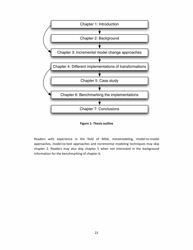
our case study. Chapter 6 gives the benchmarking results and discusses them. Chapter 7 concludes this thesis. Figure 1 shows a graphical outline of this thesis.
21
Figure 1: Thesis outline
Readers with experience in the field of MDA, metamodeling, model‐to‐model approaches, model‐to‐text approaches and incremental modeling techniques may skip chapter 2. Readers may also skip chapter 5 when not interested in the background
information for the benchmarking of chapter 6.
Chapter 1: Introduction
Chapter 2: Background
Chapter 3: Incremental model change approaches
Chapter 4: Different implementations of transformations
Chapter 5: Case study
Chapter 6: Benchmarking the implementations
Chapter 7: Conclusions

22

23
2 BACKGROUND
This chapter describes the background information about the subject
of MDE and incremental model changes. We discuss model‐to‐model transformations and model‐to‐text transformations. In the end we
also discuss state of the art MDE techniques and their capabilities of supporting incremental model changes.
2.1 INTRODUCTION An approach for software development is model driven engineering (MDE). In MDE models are not only the basis of the software under development, but also the source
code, in terms of traditional software development. Models are the leading artifacts in software development when using MDE. There are several implementations of MDE. This chapter gives more background information about the domain of MDE.
2.2 MODEL DRIVEN ARCHITECTURE
The Object Management Group (OMG) proposed Model Driven Architecture (MDA) as an implementation of MDE (Kleppe, Warmer, & Bast, 2003) (Object Management Group (OMG), 2003). MDA focuses on the creation of Platform Independent Models (PIM) and
with a PIM, together with other knowledge, performing a transformation to create Platform Specific Models (PSM). Figure 2 illustrates such a transformation. MDA describes in an abstract way how software should be developed with MDE; at a high
level the software is defined and after that, it can be transformed into a lower level with more details about the specific environment on that level, until it is executable software. The main goal of MDA is platform independence. Since software often
outlives its platform with MDA it is possible to transform a model to another platform (Object Management Group (OMG), 2003).

24
Figure 2: MDA transformation, PIM to PSM [21]
Figure 2 is intended to be suggestive and generic; the PIM and other information are
combined into a PSM and there are many ways in which such a transformation may be done (Object Management Group (OMG), 2003). Whereas the PIM is defining the subject on an abstract level, the PSM is, next to defining the same subject as the PIM,
also defining more details about the specific platform; more details about the environment. Next to the PIM to PSM transformation, MDA also describes the CIM to PIM transformation, were CIM is the Computational Independent Model. In general can
be said, the lower the level of abstraction, the more details are needed for defining the subject. Most of those lower level details are more related to the external properties of the lower level abstraction than the subject itself. The higher the level of abstraction,
the less details about the environment we need so we can be more focused on the subject itself.
Next to the PIM and PSM models, the transformations to transform a PIM to a PSM can
also be modeled in MDA. The OMG proposed Query / View / Transformation (QVT) (Object Management Group (OMG), 2007) as a transformation standard. Because of the fact that transformations themselves aro also models, they can thus also be
transformed into lower level transformations. In this way, the same transformation can be performed on each level of abstraction. Within QVT rules are described by the Object Constraint Language (OCL) (Object Management Group (OMG), 2005) also standardized
by the OMG.
PSM
PIM
Transformation
25
2.3 METAMODELING Another way of describing MDE in a more pragmatic way is as follows. Suppose we want to make a software application with a database to store information about customers.
Then the first step is to make a definition of the domain of the application we want to make. When we completed our domain we created a metamodel for our application. Metamodels define the concepts of models to be made, they propose the structure of
the models. In fact metamodels define a modeling language for models in a specific domain. Now we can make a model of our application within the just created metamodel. A metamodel defines the structure of an application and the model
contains the specific details. When the model is completed, the application should be able to run in the real world.
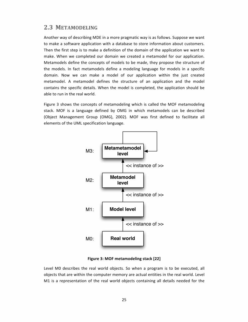
Figure 3 shows the concepts of metamodeling which is called the MOF metamodeling stack. MOF is a language defined by OMG in which metamodels can be described
(Object Management Group (OMG), 2002). MOF was first defined to facilitate all elements of the UML specification language.
Figure 3: MOF metamodeling stack [22]
Level M0 describes the real world objects. So when a program is to be executed, all objects that are within the computer memory are actual entities in the real world. Level M1 is a representation of the real world objects containing all details needed for the
Metametamodel
level
Metamodel
level
Model level
Real world
M3:
M2:
M1:
M0:
<< instance of >>
<< instance of >>
<< instance of >>

26
application to be executed in the real world. Level M2 describes the boundaries of the model in M1 and level M3 defines the concepts of metamodeling, which is self‐
descriptive. So in level M2 a domain specific language (DSL) is created whereas level M1 describes the application itself.
Figure 4 makes a comparison of MDE to the way a program written in C is constructed.
Figure 4: Comparison of the MOF stack to a program in C
As shown in Figure 4, the programming language is bound to an implementation in
EBNF. The EBNF here restricts the programmer to only use the syntax that is specific to C. The actual code is written in the C language and the real world is the compiled application. When we look at this example, the concepts of MDE are not new but are
used in many other (older) ways of software development.
Apart from performing vertical transformations in MDE, transforming models into lower level models, it is also possible to perform horizontal transformations. For example, when refining a model on level M1, a transformation can be invoked to transform the
old model into the new model staying in level M1. Both models, the old and the refined model, are still instances of the M2 level. But if there were already transformations from the old model to level M0, then the model in M0 is not an instance of our new refined
model. A new transformation has to be made to create a model in M0 which is an instance of the new refined model. This thesis focuses on transforming the model in M0
EBNF
C
Code
Real world
M3:
M2:
M1:
M0:
<< instance of >>
<< instance of >>
<< instance of >>

27
which is an instance of the old model, to a model that is an instance of the new refined model, discarding the old model in M0. In other words, we synchronize the model in M0
to the new refined model in M1.
2.4 MODEL TRANSFORMATIONS In MDE model transformations form the cornerstone in a software development process. Czarnecki and Helsen (Czarnecki & Helsen, 2003) made a classification of model
transformation approaches which we wil briefly summarize here:
There are two major categories, namely model‐to‐model and model‐to‐text. In model‐to‐text Czarnecki and Helsen define visitor‐based approaches and template‐based approaches. In template‐bases approaches templates contain already most of the text.
There are some patterns of metadata that will be replaced by data from a model. In visitor‐based approaches the visitor design pattern of Gamma et al. (Gamma, Helm, Johnson, & Vlissides, 1995) is used to transform complete models into text using, for
example, a text stream. In the model‐to‐model category Czarnecki and Helsen define direct‐manipulation approaches, relational approaches, graph‐transformation‐bases approaches, structure‐driven approaches, hybrid approaches and some other model‐to‐
model approaches. We are not discussing the model‐to‐model approaches here but this thesis focuses on the relational and the direct‐manipulation approaches. We refer to the paper of Czarnecki and Helsen for more information.
Kurtev and van den Berg (Kurtev & van den Berg, 2005) came up with a basic model
transformation pattern as illustrated in Error! Reference source not found.5.
Figure 5: The basic model transformation pattern [18]
TransformationLanguage
TransformationSpecification
Metamodel A Metamodel B
TransformationEngine
Model A Model B
source target
written in
uses uses
instance of instance ofexecuted by
input output
28
On the left hand side of Error! Reference source not found.5 we see metamodel A, on the right hand side we see metamodel B. A metamodel is a definition of a domain in
which models can be instantiated. Model A and model B represent the same data, but both in their own way. Suppose we already have model A and we want to get model B, then we need to transform our model, which is an instance of metamodel A, into a
model instance of metamodel B. Since we know metamodel A, and we know metamodel B, it is possible to make transformation rules, a transformation specification, written in a certain transformation language to process models of metamodel A and instantiate
models of metamodel B. The actual work is done by a transformation engine.
It is also possible to transform models from a certain metamodel into an instance of the same metamodel. In that way it is possible to perform model changes in an automated way.
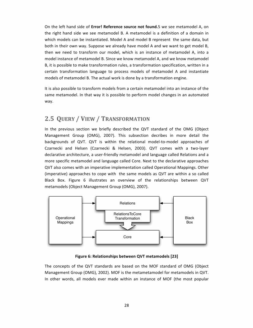
2.5 QUERY / VIEW / TRANSFORMATION In the previous section we briefly described the QVT standard of the OMG (Object Management Group (OMG), 2007). This subsection decribes in more detail the backgrounds of QVT. QVT is within the relational model‐to‐model approaches of
Czarnecki and Helsen (Czarnecki & Helsen, 2003). QVT comes with a two‐layer declarative architecture, a user‐friendly metamodel and language called Relations and a more specific metamodel and language called Core. Next to the declarative approaches
QVT also comes with an imperative implementation called Operational Mappings. Other (imperative) approaches to cope with the same models as QVT are within a so called Black Box. Figure 6 illustrates an overview of the relationships between QVT
metamodels (Object Management Group (OMG), 2007).
Figure 6: Relationships between QVT metamodels [23]
The concepts of the QVT standards are based on the MOF standard of OMG (Object Management Group (OMG), 2002). MOF is the metametamodel for metamodels in QVT.
In other words, all models ever made within an instance of MOF (the most popular
Relations
Core
OperationalMappings
BlackBox
RelationsToCoreTransformation

29
metamodel instance of MOF is UML (Object Management Group (OMG), 2003)), are able to be transformed using QVT into another model in another metamodel.
In chapter 3 of this thesis we will use the Operational Mappings part and the Relations
part of QVT to try to perform an incremental model change.
2.6 ATLAS TRANSFORMATION LANGUAGE Another approach to metamodeling, next to the QVT standard, is ATL (Jouault & Kurtev, Transforming Models with ATL, 2006). ATL is intended to be a transformation level going
beyond the QVT RFP (Object Management Group (OMG), 2002) and thus is not a direct response to that. Where QVT describes more a general approach to MDE, for example, Figure 6 does noy suggest any particular implementation of a QVT transformation
engine, ATL is more broad in terms of implementation suggestions (Jouault & Kurtev, 2005). Therefore QTL is not to be placed in the Black Box area of Figure 6. Figure 7 shows an overview of the ATL transformational approach (Jouault & Kurtev,
Transforming Models with ATL, 2006).
Figure 7: Overview of ATL transformational approach [13]
The overview of Figure 7 looks very similar to the basic transformation pattern of Error! Reference source not found. 5. In ATL the transformation specification is a model instance of the metamodel (language) ATL. In ATL the notion instance of is called
conforms to because they state that models are not real instantiations of their
ATL
mmA2mmB.atl
Metamodel A Metamodel B
Model A Model Bsource target
MOF
conforms to
transformation
executes

30
metamodel (like objects are of classes in OO development), but models are conforming to a specification; both the metamodels and models are instances themselves (Bézivin,
2005).
ATL is a hybrid transformation language in which it is possible to use both declarative and imperative constructs. It can be compared to QVT Operational Mappings. ATL is, just as QVT, within the relational model‐to‐model approaches of Czarnecki and Helsen
(Czarnecki & Helsen, 2003).
In chapter 3 of this thesis we will use ATL to try to perform an incremental model change. There we will conclude wheter or not the transformation language is suitable for our purpose.
2.7 INCREMENTAL MODEL TRANSFORMATIONS Hearnden et al. (Hearnden, Lawley, & Raymond, 2006) states that there are two approaches to incremental updates, which we call incremental model changes. Figure 8 and Figure 9 illustrate those two approaches.
Figure 8: Re‐transformation [11]
First we map Figure 8 on a real life example. This example also holds for Figure 9, Figure 10 and Figure 11. We define S as the source model and T as the instance of that model in the file system of a computer, so called files. With delta S we transform the source
model to its successor. The transformation to the file system is called t. In the next figures we also have delta T which transforms T to its successor.
Hearden et al. (Hearnden, Lawley, & Raymond, 2006) mention the re‐transformation in Figure 8. In this approach to incremental model transformation the only artifact that will

31
be updated incrementally is the source model. All model elements will be transformed into files in the file system where merging has to take place to perform an incremental
update. On first sight this could cause a lot of overhead because not all files have to be re‐generated with a particular delta. We will take a closer look to this approach in chapter 4.
Figure 9: Live transformation [11]
Another approach Hearden et al. (Hearnden, Lawley, & Raymond, 2006) mentioned is the live transformation illustrated in Figure 9. This approach uses a continuous transformation to directly update the file system if a single change has happened at the
source model. The delta of the source model will be transformed into a delta for the file system and the files that are concerned with this change will be updated. A disadvantage of this approach is that there must be a constant link with the file system,
which is in some cases not always possible, for instance when working via a network or internet. Another disadvantage is that a lot of transformations have to be maintained, which is not always preferred. Because of both disadvantages we do not take a closer
look at this approach in this thesis.
Next to the approach of Figure 8 we do take a closer look at the approaches we defined ourselves, and which we discuss later in this thesis, in Figure 10 and Figure 11.
32
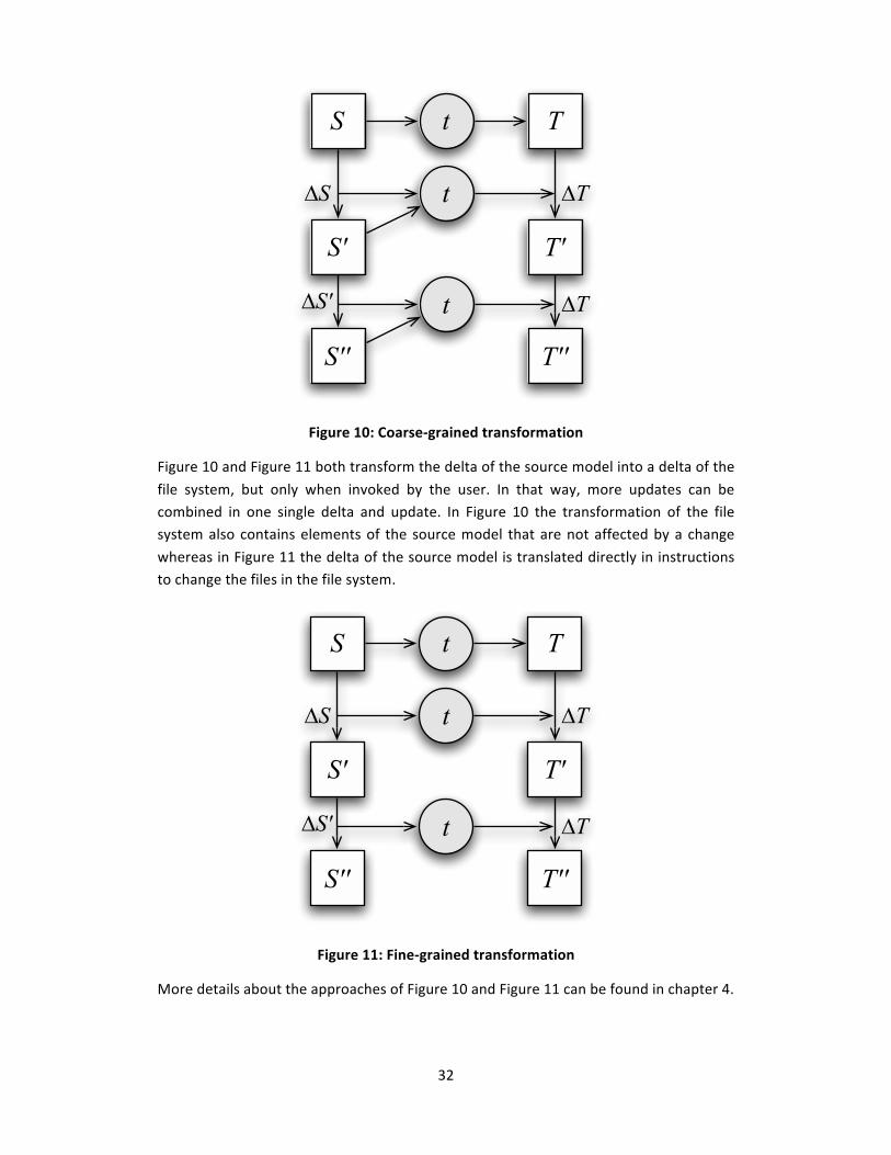
Figure 10: Coarse‐grained transformation
Figure 10 and Figure 11 both transform the delta of the source model into a delta of the
file system, but only when invoked by the user. In that way, more updates can be combined in one single delta and update. In Figure 10 the transformation of the file system also contains elements of the source model that are not affected by a change
whereas in Figure 11 the delta of the source model is translated directly in instructions to change the files in the file system.
Figure 11: Fine‐grained transformation
More details about the approaches of Figure 10 and Figure 11 can be found in chapter 4.
33
2.8 MODELTOTEXT TRANSFORMATIONS In the previous sections we talked about model transformations, those are actually model‐to‐model transformations. In this section we introduce model‐to‐text
transformations. In model‐to‐text a model is being transformed to a textual representation, for example, to files in a file system.
When using models to develop software we need to have some platform to be able to execute the software. An approach is to have a runtime environment in which models
can be executed (executable models), another approach is to generate code from the models (model‐to‐text) that can be compiled using traditional programming tools. The difference between the two is that in model‐to‐text a programmer has full control over
the generated code before it is being compiled. This is a huge advantage over the executable model approach because a runtime environment needs to give full support for all behaviour of the application. When in model‐to‐text some behaviour cannot be
modeled, a programmer can add the behaviour afterwards by changing the generated code. With executable models a programmer does not only have to add behaviour to the runtime environment, but also to the metamodel of the model that has to be
executed. Next to that, also in the model itself the behaviour has to be added so it can be executed. Here we see that at three different levels changes have to be made to support new behaviour. In the model‐to‐text approach we only need to change the
generated code. When the same behaviour is added over and over again afterwards, one could think of adding the behaviour to the metamodel and code generator to support the behaviour for the next time. This gives flexibility to the user. For the same
reason tool vendors in the industry use code generation rather than executable models (Novulo, 2009).
Other approaches in the field of model‐to‐text that we did not study are, for example, MOFScript (Oldevik, 2009) and openArchitectureWare (Efftinge, et al., 2008). Both
approaches are based on the EMF platform (Steinberg, Budinsky, Paternostro, & Merks, 2008). We did not study those approaches because we first needed to know how an incremental model change could be performed. We first wanted to study existing
model‐to‐model approaches, but since we encountered (in chapter 3) that the approaches that we studied were not sufficient for our needs, we started developing an own proposal and thus we were automatically bounded to our own approach in which
we, next to a model‐to‐model approach, also defined a model‐to‐text approach. Now the concepts of this thesis are clear, future research should turn out if our approach to incremental model changes could also be performed in approaches such as MOFScript
and openArchitectureWare.
34
2.9 RELATED WORK Könemann (Könemann, Kindler, & Unland, 2009) defined an approach for model synchronization in a similar way as we will present in this thesis. Like our approach, they
use deltas to perform transformations. Where we try to keep the model and generated code synchronized, they try to keep an analysis model and a design model synchronized. The analysis model is the model that will be changed where in our approach we only
have one model and that model will be changed.
An important difference in the approach of Könemann and ours is the construction of the delta. We state that the elements of delta will be collected as an ongoing process while a modeler changes a source model. The tool that provides the modeling
environment should monitor the changes in the source model and collect them in a delta. Könemann states that there are already two different versions of one model (which then are of course two models, but they represent the same application) and the
delta will be extracted from both versions. They also distuinguish between symmetric and directed deltas. Symmetric deltas are able two perform a bi‐directional transformation, this means that when, for example, a delta is constructed of a model
version 1 and version 2, we could perform a transformation to obtain version 2 from version 1 and also version 1 from version 2. A directed delta will only be able to obtain version 2 from version 1, which is uni‐directional. In our thesis we are only interested in
the uni‐directional approach (e.g., from version 1 to version 2) since in our approach we perform code generation and a modeler is always allowed to open a previous version of the model and perform an entire model transformation to generate the code of that
version (again).
Another difference between the approaches of Könemann and ours is the set of operations. We state that there are three distinct types of transformation operations (atomic changes called by Könemann), namely additions, changes and deletions.
Könemann states that there are four, namely additions, changes, deletions and movements. We perform a movement by performing an addition and a deletion subsequently. Properties and references of the entity to be deleted will be copied and
the id‐values of the entities referring to the entity to be deleted will be changed to the added entity.
A third difference is the metamodel to which the delta will be conforming to. Könemann defined a general metamodel for the delta. The delta in our approach is conforming to
the metamodel of the source model. The difference is that in the approach of Könemann they have to address every type of change per entity, including additions. In our approach this is clear because when an entity exists in the delta and not in the
target model (in model‐to‐model approach), it is obviously an addition. We did not compare the different approaches in this thesis so we cannot state which solution is the
most efficient. This is an issue for further research.

35
An important similarity in the approach of Könemann and ours is the distinction between model‐dependent and model‐independent deltas as stated by Könemann. We
do not emphasize this distinction since in our case is not very important. In Könemann’s approach they want to obtain a design model from a previous version of the design model with a delta. In their case it is important to know whether the delta needs the
original analysis model for the transformation or not. When it does, they call this model‐dependency, when it doesn’t, they call it model‐independency. In our case we have two model‐dependent approaches and one semi‐model‐independent approach. We state
semi, because in some cases it is model‐dependent. In section 4.4 of chapter 4 we will clarify our statement since by then the concepts of our three approaches are clear.
2.10 CONCLUSION In the previous sections we described the general concept of MDA, we introduced the
concepts of metamodeling and discussed model transformations. For model transformations we first summarized the classification of model transformation approaches and also briefly introduced the model transformation approaches QVT and
ATL. For model transformation, both model‐to‐model and model‐to‐text, we defined several approaches to perform incremental model changes. This concepts we will use in further chapters of this thesis. We also introduced to model‐to‐text transformations in
this chapter, this thesis will state that there are significant differences between model‐to‐model and model‐to‐text and it should not be underestimated. We conclude this chapter with a section about related work in this field.

36
37
3 INCREMENTAL MODEL CHANGE APPROACHES
“Problems with the waterfall model have been recognized for a long time. The emphasis in the waterfall model is on documents and writing. Fred Brooks (The Mythical Man Month, Anniversary Edition,
1995, page 200): “I still remember the jolt I felt in 1958 when I first heard a friend talk about building a program, as opposed to writing one”. The “building” metaphor led to many new ideas: planning;
specification as blueprint; components; assembly; scaffolding; etc. But the idea that planning preceded construction remained. In 1971, Harlan Mills (IBM) proposed that we should grow software rather
than build it. We begin by producing a very simple system that runs but has minimal functionality and then add to it and let it grow. Ideally, the software grows like a flower or a tree; occasionally,
however, it may spread like weeds. The fancy name for growing software is incremental development.”
(Paquet, 2009)
3.1 INTRODUCTION We start this chapter with the background information define the boundaries of the
subject. Next we give examples of model‐to‐model transformations within state of the art model transformation techniques and in the end we conclude this chapter with an own incremental model‐to‐model and model‐to‐text transformation algorithm.
Section 3.2 discusses the field in which incremental model changes are desirable. We
discuss how model transformations work and which types of transformations are possible. Section 3.3 discusses implementations of the different types of transformations, what have been discussed in section 3.2, within several state of the art
model transformation techniques. Section 3.4 discusses an approach to perform an incremental model change. We propose an algorithm that is able to perform the different types of transformations discussed in section 3.2. We support our proposal by
a code listing and a sample transformation. We conclude this chapter with section 3.5.
38
3.2 MODEL TRANSFORMATIONS When performing a model transformation we always have a source model and a target model. The complexity of the transformation depends on the changes in hierarchy that
have to be made. This is of course depending on the metamodel. When both source and target models are within the same metamodel, the transformation will be very straightforward. In case of different metamodels the transformation could get more
complex.
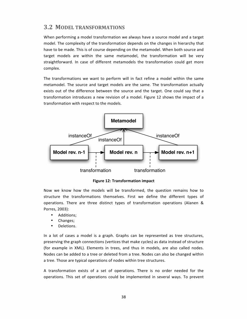
The transformations we want to perform will in fact refine a model within the same metamodel. The source and target models are the same. The transformation actually exists out of the difference between the source and the target. One could say that a
transformation introduces a new revision of a model. Figure 12 shows the impact of a transformation with respect to the models.
Figure 12: Transformation impact
Now we know how the models will be transformed, the question remains how to structure the transformations themselves. First we define the different types of
operations. There are three distinct types of transformation operations (Alanen & Porres, 2003):
• Additions; • Changes; • Deletions.
In a lot of cases a model is a graph. Graphs can be represented as tree structures, preserving the graph connections (vertices that make cycles) as data instead of structure (for example in XML). Elements in trees, and thus in models, are also called nodes.
Nodes can be added to a tree or deleted from a tree. Nodes can also be changed within a tree. Those are typical operations of nodes within tree structures.
A transformation exists of a set of operations. There is no order needed for the operations. This set of operations could be implemented in several ways. To prevent
Model rev. nModel rev. n-1 Model rev. n+1
transformation transformation
Metamodel
instanceOfinstanceOf
instanceOf
39
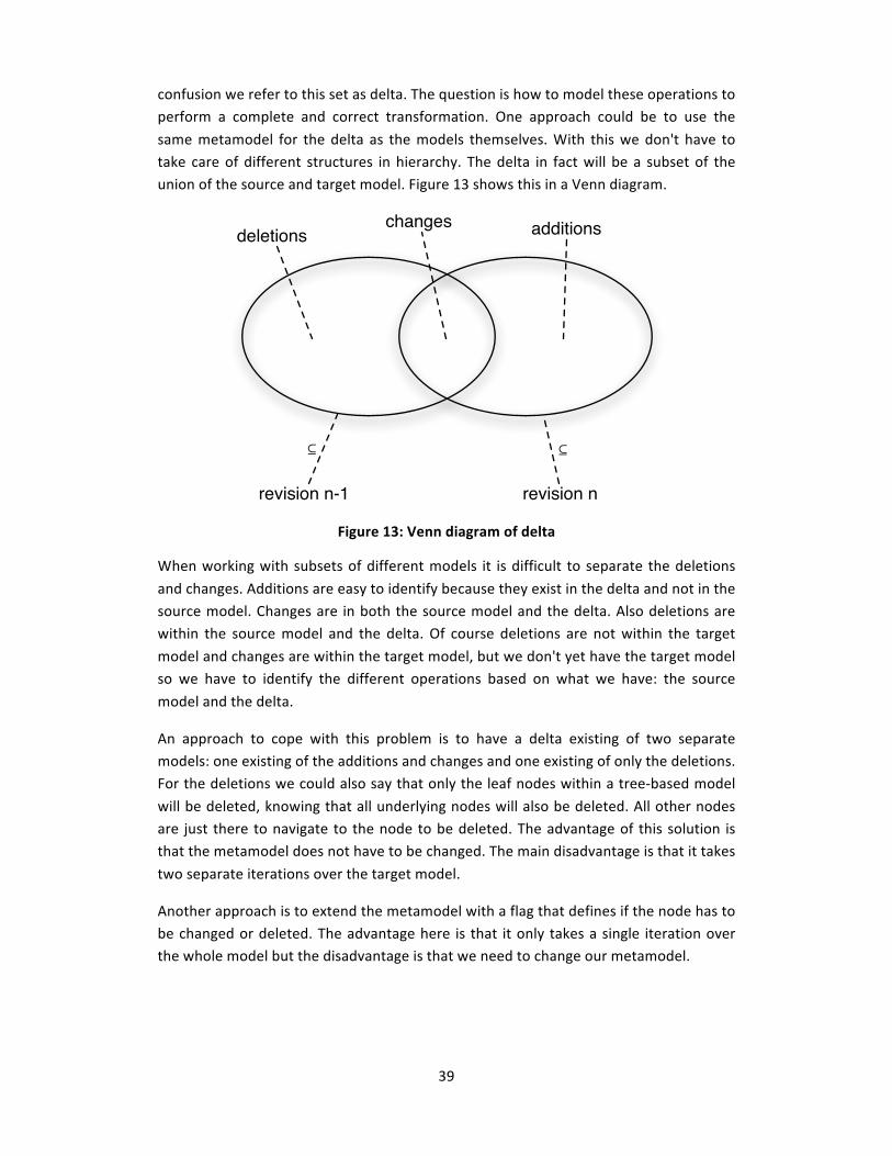
confusion we refer to this set as delta. The question is how to model these operations to perform a complete and correct transformation. One approach could be to use the
same metamodel for the delta as the models themselves. With this we don't have to take care of different structures in hierarchy. The delta in fact will be a subset of the union of the source and target model. Figure 13 shows this in a Venn diagram.
Figure 13: Venn diagram of delta
When working with subsets of different models it is difficult to separate the deletions
and changes. Additions are easy to identify because they exist in the delta and not in the source model. Changes are in both the source model and the delta. Also deletions are within the source model and the delta. Of course deletions are not within the target
model and changes are within the target model, but we don't yet have the target model so we have to identify the different operations based on what we have: the source
model and the delta.
An approach to cope with this problem is to have a delta existing of two separate models: one existing of the additions and changes and one existing of only the deletions. For the deletions we could also say that only the leaf nodes within a tree‐based model
will be deleted, knowing that all underlying nodes will also be deleted. All other nodes are just there to navigate to the node to be deleted. The advantage of this solution is that the metamodel does not have to be changed. The main disadvantage is that it takes
two separate iterations over the target model.
Another approach is to extend the metamodel with a flag that defines if the node has to be changed or deleted. The advantage here is that it only takes a single iteration over the whole model but the disadvantage is that we need to change our metamodel.
deletionschanges additions
! !
revision n-1 revision n

40
3.3 STATE OF THE ART MODEL TRANSFORMATION TECHNIQUES State of the art model transformation techniques are currently a heavy topic of research due to, for example, the Query/View/Transformations (QVT) request for proposal (RFP)
by the OMG (Object Management Group (OMG), 2002). Another contribution is for example the Atlas Transformation Language (ATL) (Jouault & Kurtev, Transforming Models with ATL, 2006). This section discusses approaches of incremental model
changes in QVT and ATL. In QVT we used QVT Relations and QVT Operational Mappings because of the different paradigms. QVT Relations is a declarative language and QVT Operational Mappings is both declarative and imperative.
In both QVT and ATL it is possible to define a transformation that is able to transform a
model that conforms to a certain metamodel, into a model that conforms to another metamodel. We are concerned about making a transformation within the same metamodel which keeps the transformation straightforward.
3.3.1 EXAMPLE TRANSFORMATIONS Within the next sections 3.3.2, 3.3.3 and 3.3.4 we discuss how several types of deltas
could be processed in state of the art model transformation techniques. This section introduces the deltas that will be used in the next sections.
Figure 14: Subset of delta that contains two additions
Within Figure 14 node 5 and node 6 will be added. Node 4 should already exist in the source model because the rules will check whether the current node that is processed
contains an attribute id with its value set to 4. For the example it does not matter what the model looks like above the level of node 4.
5
6
4
...
41
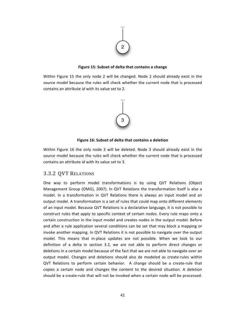
Figure 15: Subset of delta that contains a change
Within Figure 15 the only node 2 will be changed. Node 2 should already exist in the
source model because the rules will check whether the current node that is processed contains an attribute id with its value set to 2.
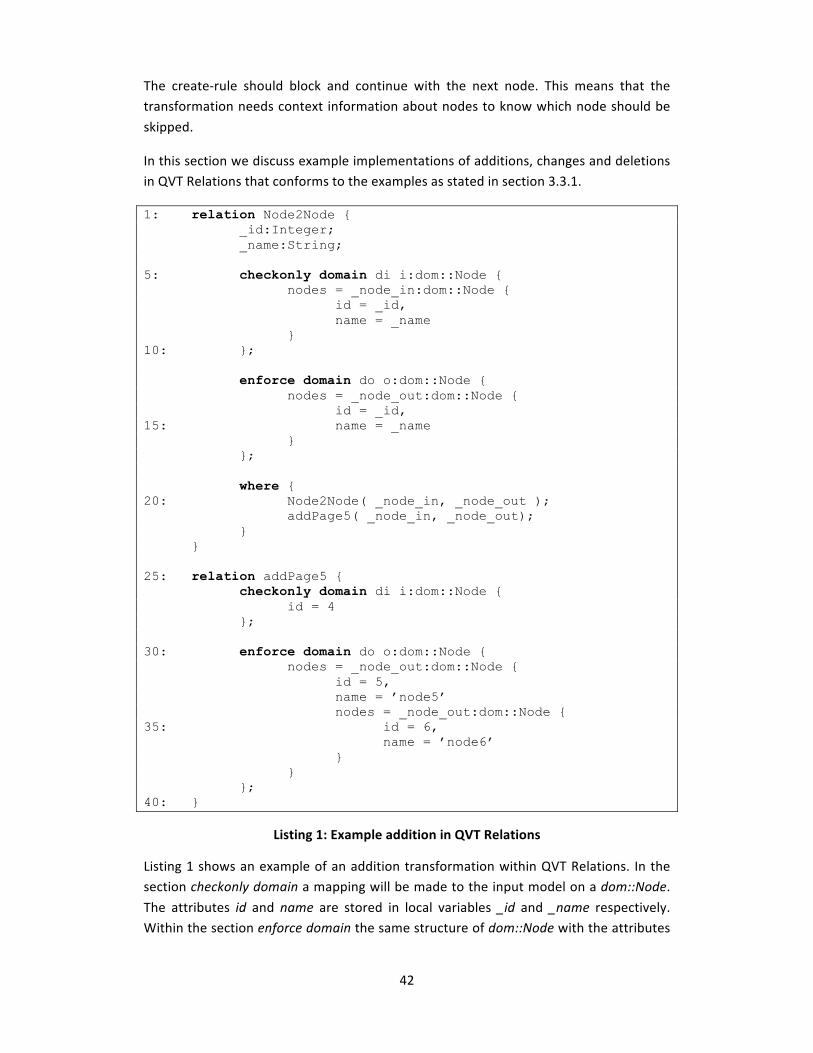
Figure 16: Subset of delta that contains a deletion
Within Figure 16 the only node 3 will be deleted. Node 3 should already exist in the source model because the rules will check whether the current node that is processed
contains an attribute id with its value set to 3.
3.3.2 QVT RELATIONS One way to perform model transformations is by using QVT Relations (Object Management Group (OMG), 2007). In QVT Relations the transformation itself is also a model. In a transformation in QVT Relations there is always an input model and an
output model. A transformation is a set of rules that could map onto different elements of an input model. Because QVT Relations is a declarative language, it is not possible to
construct rules that apply to specific context of certain nodes. Every rule maps onto a certain construction in the input model and creates nodes in the output model. Before and after a rule application several conditions can be set that may block a mapping or
invoke another mapping. In QVT Relations it is not possible to navigate over the output model. This means that in‐place updates are not possible. When we look to our definition of a delta in section 3.2, we are not able to perform direct changes or
deletions in a certain model because of the fact that we are not able to navigate over an output model. Changes and deletions should also de modeled as create‐rules within QVT Relations to perform certain behavior. A change should be a create‐rule that
copies a certain node and changes the content to the desired situation. A deletion should be a create‐rule that will not be invoked when a certain node will be processed.
2
...
3
...
42
The create‐rule should block and continue with the next node. This means that the transformation needs context information about nodes to know which node should be
skipped.
In this section we discuss example implementations of additions, changes and deletions in QVT Relations that conforms to the examples as stated in section 3.3.1.
1: relation Node2Node { _id:Integer; _name:String; 5: checkonly domain di i:dom::Node { nodes = _node_in:dom::Node { id = _id, name = _name } 10: }; enforce domain do o:dom::Node { nodes = _node_out:dom::Node { id = _id, 15: name = _name } }; where { 20: Node2Node( _node_in, _node_out ); addPage5( _node_in, _node_out); } } 25: relation addPage5 { checkonly domain di i:dom::Node { id = 4 }; 30: enforce domain do o:dom::Node { nodes = _node_out:dom::Node { id = 5, name = ’node5’ nodes = _node_out:dom::Node { 35: id = 6, name = ’node6’ } } }; 40: }
Listing 1: Example addition in QVT Relations
Listing 1 shows an example of an addition transformation within QVT Relations. In the section checkonly domain a mapping will be made to the input model on a dom::Node.
The attributes id and name are stored in local variables _id and _name respectively. Within the section enforce domain the same structure of dom::Node with the attributes

43
id and name is created with the values stored in the local variables before. The where clause invokes besides a call to Node2Node to process the next node, a call to
addPage5. The relation addPage5 checks in the section checkonly domain whether the incoming node has the attribute id set to the value 4. When this holds the section enforce domain will create a dom::Node as a child of the current node (with id equal to
4) together with a new name and a child of its own. So in fact two nodes are added here to an existing model. It is also possible to make the function addPage5 more general with three parameters to make a variable checkonly domain and variable attributes for
the newly created node(s) in enforce domain, but for simplicity we only present the specific implementation. Figure 14 shows the delta that conforms to this transformation.
1: relation Node2Node { _id:Integer; _name:String; 5: checkonly domain di i:dom::Node{ nodes = _node_in:dom::Node { id = _id, name = _name } 10: }; enforce domain do o:dom::Node{ nodes = _node_out:dom::Node { id = _id, 15: name = if ( id = 2 ) then ’changed_name’ else _name endif } }; 20: where{ Node2Node( _node_in, _node_out ); } }
Listing 2: Example change in QVT Relations
Listing 2 shows an example of a change transformation within QVT Relations. The checkonly domain here is exactly the same as for an addition. The difference is within the enforce domain and within the where clause. Within the enforce domain a new
dom::Node will be created but when the attribute name will be filled, an OCL expression is made to check if the current node we handle has its attribute id set to 2. When this is
the case, the name attribute will not be copied from the input model but instead, the value "changed_name" will be assigned. Within the where clause only a call to Node2Node will be made to process the next node. Figure 15 shows the delta that
conforms to this transformation.
44
1: relation Node2Node { _id:Integer; _name:String; _next_id:Integer; 5: checkonly domain di i:dom::Node { nodes = _node_in:dom::Node { id = _id, name = _name, 10: nodes = _next_node_in:dom::Node { id = _next_id } } }; 15: enforce domain do o:dom::Node { nodes = _node_out:dom::Node { id = _id, name = _name 20: } }; primitive domain del:Integer; 25: when { if ( del = 3 ) then false else true endif; } where{ 30: Node2Node( _node_in, _node_out, _next_id ); } }
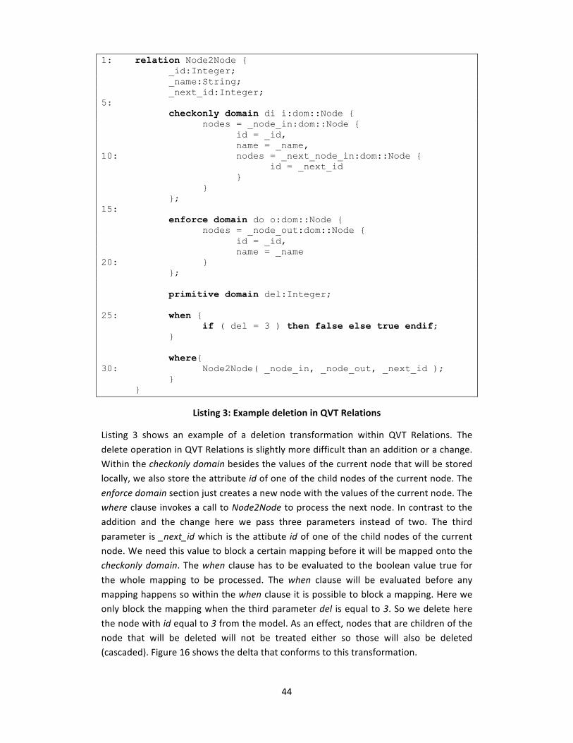
Listing 3: Example deletion in QVT Relations
Listing 3 shows an example of a deletion transformation within QVT Relations. The
delete operation in QVT Relations is slightly more difficult than an addition or a change. Within the checkonly domain besides the values of the current node that will be stored locally, we also store the attribute id of one of the child nodes of the current node. The
enforce domain section just creates a new node with the values of the current node. The where clause invokes a call to Node2Node to process the next node. In contrast to the addition and the change here we pass three parameters instead of two. The third
parameter is _next_id which is the attibute id of one of the child nodes of the current node. We need this value to block a certain mapping before it will be mapped onto the checkonly domain. The when clause has to be evaluated to the boolean value true for
the whole mapping to be processed. The when clause will be evaluated before any mapping happens so within the when clause it is possible to block a mapping. Here we only block the mapping when the third parameter del is equal to 3. So we delete here
the node with id equal to 3 from the model. As an effect, nodes that are children of the node that will be deleted will not be treated either so those will also be deleted (cascaded). Figure 16 shows the delta that conforms to this transformation.

45
In listing 1, listing 2 and listing 3 we included sample code in QVT Relations that perform actions that could be in a delta. When performing such a transformation the result is a
separate model so we do not perform a real incremental model change because we don't actually change an existing model. As stated before, in QVT Relations it is not possible navigate over the output model and that is a prerequisite to perform an
incremental model change.
3.3.3 QVT OPERATIONAL MAPPINGS
Another approach next to QVT Relations but still within the QVT concept is QVT Operational Mappings (Object Management Group (OMG), 2007). QVT Operational Mappings is both a declarative and an imperative language, in contrast to QVT
Relations, which is only a declarative language.
In this section we discuss example implementations of additions, changes and deletions in QVT Operational Mappings that conforms to the examples as stated in section 3.3.1.
1: mapping Node::Node::traverse() : Node::Node init { var x : OrderedSet(Node::Node) := self.getNodes(); 5: x := if ( self.id = 4 ) then x->append( createNode( 5, 'node' ) )->asOrderedSet() else 10: x endif; } id := self.id; 15: name := self.name; nodes := x; } helper createNode( _id:Integer, _name:String ) : Node::Node 20: { var x : OrderedSet(Node::Node) := null; x := if ( _id = 5 ) then if ( x = null ) then 25: createNode( 6, 'node' )->asOrderedSet() else x->append( createNode( 6, 'node' ) ) endif else 30: x endif; return object Node::Node { id := _id; 35: name := _name+' '+_id.toString();
46
nodes := x; } } 40: query Node::Node::getNodes() : OrderedSet(Node::Node) { return self.nodes->asOrderedSet()->collect( s | s.map traverse() )->asOrderedSet(); }
Listing 4: Example addition in QVT Operational Mappings
Listing 4 shows an example of an addition in QVT Operational Mappings. The actual rule
mapping happens in the mapping section. This is a function on which all nodes of the type Node::Node map. The first step in the rule mapping is the collection of all child nodes of the current node. The function getNodes collects those child nodes and is
declared in the first query section. It also invokes the traverse function on all child nodes. When a node passes which has its id attribute set to 4 then the collection of child nodes will be extended with a new node constructed by createNode. Within the helper
section createNode is declared and implemented. The helper looks similar like the mapping section but here it returns a newly constructed Node::Node object. It also does a recursive call to construct a new child node directly in the node to be constructed. The
stop‐case for the recursive call is the if‐statement that checks whether the id attribute of the to be constructed node is equal to 5, which is only the case in the first call. Figure 14 shows the delta that conforms to this transformation.
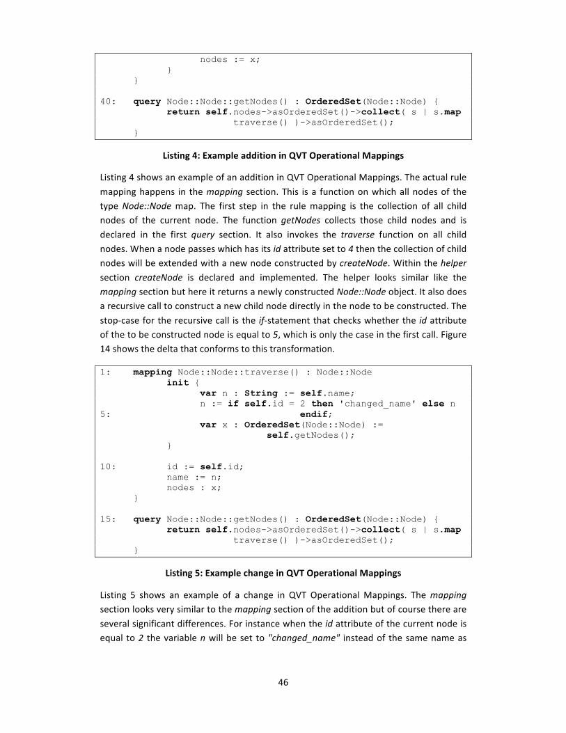
1: mapping Node::Node::traverse() : Node::Node init { var n : String := self.name; n := if self.id = 2 then 'changed_name' else n 5: endif; var x : OrderedSet(Node::Node) := self.getNodes(); } 10: id := self.id; name := n; nodes : x; } 15: query Node::Node::getNodes() : OrderedSet(Node::Node) { return self.nodes->asOrderedSet()->collect( s | s.map traverse() )->asOrderedSet(); }
Listing 5: Example change in QVT Operational Mappings
Listing 5 shows an example of a change in QVT Operational Mappings. The mapping section looks very similar to the mapping section of the addition but of course there are
several significant differences. For instance when the id attribute of the current node is equal to 2 the variable n will be set to "changed_name" instead of the same name as
47
the current value of the mapped node. In the end the name attribute of the node that will be present in the output model will be assigned to n. Figure 15 shows the delta that
conforms to this transformation.
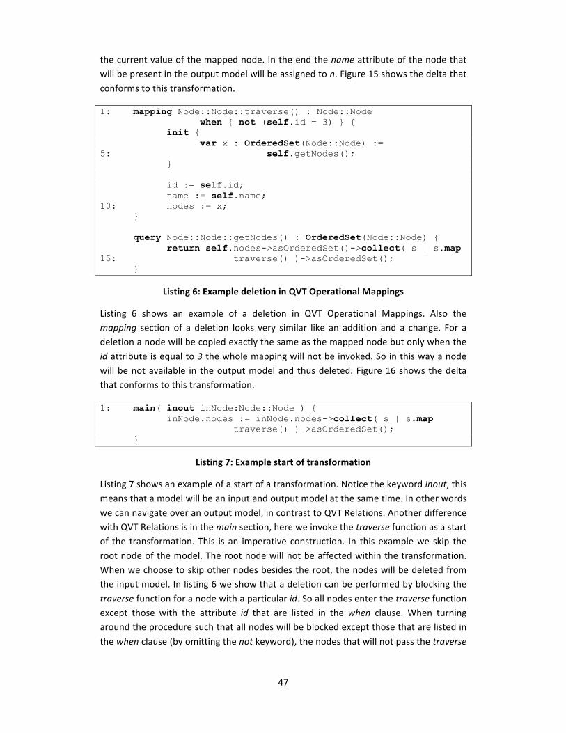
1: mapping Node::Node::traverse() : Node::Node when { not (self.id = 3) } { init { var x : OrderedSet(Node::Node) := 5: self.getNodes(); } id := self.id; name := self.name; 10: nodes := x; } query Node::Node::getNodes() : OrderedSet(Node::Node) { return self.nodes->asOrderedSet()->collect( s | s.map 15: traverse() )->asOrderedSet(); }
Listing 6: Example deletion in QVT Operational Mappings
Listing 6 shows an example of a deletion in QVT Operational Mappings. Also the mapping section of a deletion looks very similar like an addition and a change. For a deletion a node will be copied exactly the same as the mapped node but only when the
id attribute is equal to 3 the whole mapping will not be invoked. So in this way a node will be not available in the output model and thus deleted. Figure 16 shows the delta that conforms to this transformation.
1: main( inout inNode:Node::Node ) { inNode.nodes := inNode.nodes->collect( s | s.map traverse() )->asOrderedSet(); }
Listing 7: Example start of transformation
Listing 7 shows an example of a start of a transformation. Notice the keyword inout, this means that a model will be an input and output model at the same time. In other words
we can navigate over an output model, in contrast to QVT Relations. Another difference with QVT Relations is in the main section, here we invoke the traverse function as a start of the transformation. This is an imperative construction. In this example we skip the
root node of the model. The root node will not be affected within the transformation. When we choose to skip other nodes besides the root, the nodes will be deleted from the input model. In listing 6 we show that a deletion can be performed by blocking the
traverse function for a node with a particular id. So all nodes enter the traverse function except those with the attribute id that are listed in the when clause. When turning around the procedure such that all nodes will be blocked except those that are listed in
the when clause (by omitting the not keyword), the nodes that will not pass the traverse

48
function will also be deleted. We can conclude that all nodes in the input model will be affected in the transformation, also those that are blocked by a when clause. With this
property it is impossible to perform an incremental model change with only affecting those elements that are actually changed.
According to the final adopted specification of QVT (Object Management Group (OMG), 2007), QVT Operational Mappings supports the ability to remove nodes from a model
with the so called removeElement function. This would only be meaningful when performing a model transformation where the input and output models are the same, using the keyword inout, because then we can only delete the nodes we desire, and
leave the rest untouched. But since all nodes have to be visited when performing a model transformation, even when using the keyword inout, the removal of nodes can also be inferred by skipping the visitation of certain nodes, as shown in listing 6.
3.3.4 ATL ATL (Jouault & Kurtev, Transforming Models with ATL, 2006) is like QVT Relations a
hybrid imperative and declarative language. Function calls are either blocked or allowed. When blocked, the node will be deleted in the output model. In ATL it is possible to use the same input file as the output file, just like QVT Operational
Mappings.
In this section we discuss example implementations of additions, changes and deletions in ATL that conforms to the examples as stated in section 3.3.1.
1: rule Node { from i : Node!Node to 5: o : Node!Node ( id <- i.id, name <- i.name, nodes <- if i.id = 4 then i.nodes->including( 10: thisModule.NewNode( 5, 'node 5' ) ) else 15: i.nodes endif ) } 20: rule NewNode ( _id : Integer, _name : String ) { to o : Node!Node ( id <- _id, name <- _name, 25: nodes <- if _id = 5 then
49
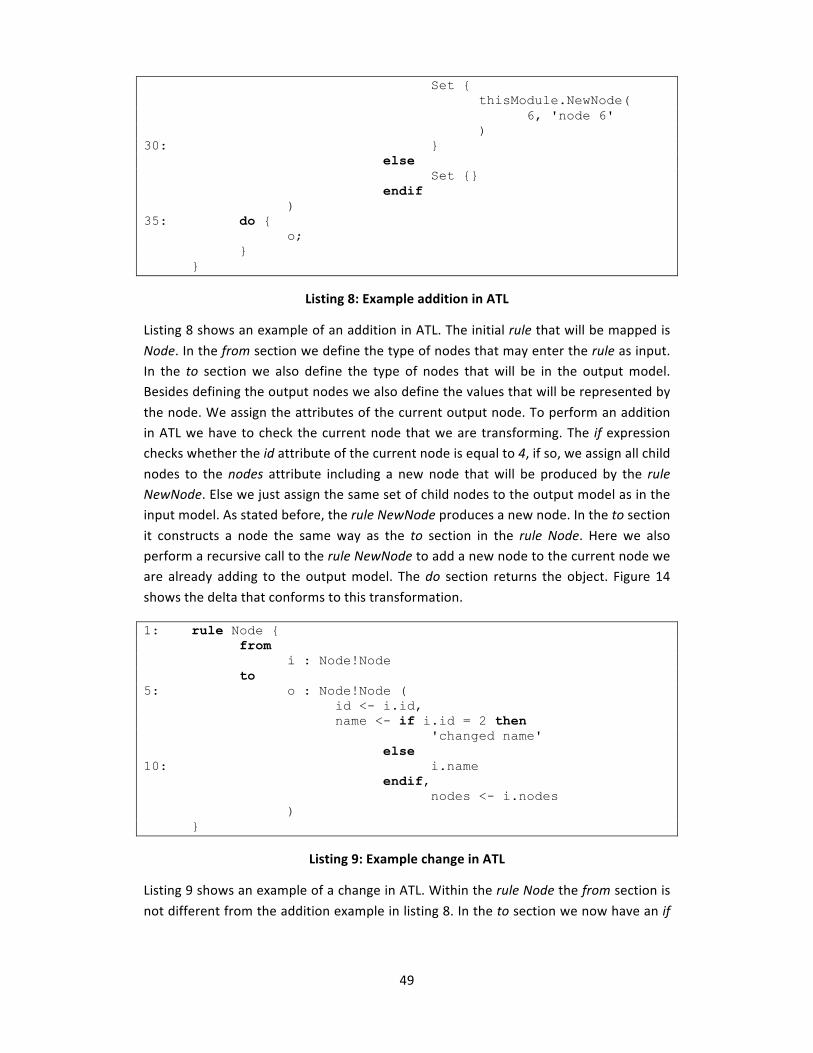
Set { thisModule.NewNode( 6, 'node 6' ) 30: } else Set {} endif ) 35: do { o; } }
Listing 8: Example addition in ATL
Listing 8 shows an example of an addition in ATL. The initial rule that will be mapped is
Node. In the from section we define the type of nodes that may enter the rule as input. In the to section we also define the type of nodes that will be in the output model. Besides defining the output nodes we also define the values that will be represented by
the node. We assign the attributes of the current output node. To perform an addition in ATL we have to check the current node that we are transforming. The if expression checks whether the id attribute of the current node is equal to 4, if so, we assign all child
nodes to the nodes attribute including a new node that will be produced by the rule NewNode. Else we just assign the same set of child nodes to the output model as in the input model. As stated before, the rule NewNode produces a new node. In the to section
it constructs a node the same way as the to section in the rule Node. Here we also perform a recursive call to the rule NewNode to add a new node to the current node we are already adding to the output model. The do section returns the object. Figure 14
shows the delta that conforms to this transformation.
1: rule Node { from i : Node!Node to 5: o : Node!Node ( id <- i.id, name <- if i.id = 2 then 'changed name' else 10: i.name endif, nodes <- i.nodes ) }
Listing 9: Example change in ATL
Listing 9 shows an example of a change in ATL. Within the rule Node the from section is
not different from the addition example in listing 8. In the to section we now have an if

50
expression at the attribute name to check whether the current node we are transforming has the attribute id equal to 2. If so, we change the name attribute to
"changed_name" else we leave the value the same as the input model. Figure 15 shows the delta that conforms to this transformation.
1: rule Node { from i : Node!Node ( not (i.id = 3) ) to 5: o : Node!Node ( id <- i.id, name <- i.name, nodes <- i.nodes ) 10: }
Listing 10: Example deletion in ATL
Listing 10 shows an example of a deletion in ATL. The from section in the rule Node has a precondition. It will block when the attribute id of the current node is equal to 3. This
will cause the node to be deleted in the output model. If the current node does not have its attribute id equal to 3, it will enter the to section. In the to section all attributes from the input node will be copied to the output node. Figure 16 shows the delta that
conforms to this transformation.
The philosophy of ATL is that input and output models are separate models. ATL supports model refinements, but instead of refining the input model, ATL will copy the input model to an output model and then refine the output model. The input model is
always read‐only while the output model is write‐only. Output models cannot be navigated (Jouault & Kurtev, Transforming Models with ATL, 2006).
3.3.5 SUMMARY In this section we studied three state of the art model transformation techniques. We studied several ways to implement additions, changes and deletions within the
transformation languages. For each model driven technique we found ways to implement the required operations. To use the model transformation techniques for incremental model changes some more requirements are needed. We summarized
several properties of the transformation languages in table 1.
In‐model changes
Partial model processing
Supporting model‐to‐text transformations
QVT Relations No No No QVT Operational Mappings Yes No No ATL No No No
Table 1: Properties of state of the art model transformation techniques
51
The properties presented in table 1 are:
• In‐model changes
In‐model changes state whether it is possible to store changes in the same model as the input model. It turned out that only QVT Operational Mappings is able to perform such a
transformation: a model refinement. ATL may simulate this by applying an automatic copy mechanism. The results we retrieved were also described by Grammel and Voigt (Grammel & Voigt, 2009). Grammel and Voigt stated that the VIATRA (Csertán, Huszerl,
Majzik, Pap, Pataricza, & Varró, 2002) transformation language was capable of performing in‐model changes. Further research should turn out if it also suits our needs.
• Partial model processing
Partial model processing states whether it is possible to only process a part of the input model while outputting a complete model including the part of the input model that
was not processed during the partial model process. This means that it is only possible when in‐model changes are allowed, since we cannot know the rest of the model.
A successful model transformation language for incremental model changes should support in‐model changes together with partial model processing. Since none of the
state of the art model transformation techniques we studied support both properties, the need for a new proposal rises.
• Supporting model‐to‐text transformations
Another reason to define a new proposal for incremental model changes is because the incremental changes do not only affect models, but also files. Besides making an
incremental model‐to‐model transformation we are also concerned with an incremental model‐to‐text transformation.
3.4 OUR PROPOSAL This section describes a pseudo algorithm to implement the proposed approach. This
chapter contains a conceptual description of the algorithm and also code fragments to support the concept together with images. The code fragments are written in an imperative pseudo language. Here we define a direct‐manipulation approach which is
described by Czarnecki and Helsen (Czarnecki & Helsen, 2003).
Suppose we have a model called source. This model is the main model in our algorithm. The source model always starts as an empty model. This means that the first delta always contains additions. In this way the initial transformation does not differ in any
aspect from any further transformations. When the source model is not empty anymore we are able to also change or delete certain elements. Additions, changes and deletions
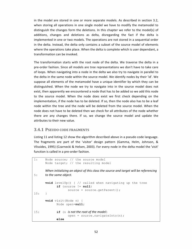
52
in the model are stored in one or more separate models. As described in section 3.2, when storing all operations in one single model we have to modify the metamodel to
distinguish the changes form the deletions. In this chapter we refer to the model(s) of additions, changes and deletions as delta, disregarding the fact if the delta is implemented in one or two models. The operations are not stored in a sequential order
in the delta. Instead, the delta only contains a subset of the source model of elements where the operations take place. When the delta is complete which is user dependant, a transformation can be invoked.
The transformation starts with the root node of the delta. We traverse the delta in a
pre‐order fashion. Since all models are tree representations we don't have to take care of loops. When navigating into a node in the delta we also try to navigate in parallel to the delta in the same node within the source model. We identify nodes by their 'id'. We
suppose all elements of the metamodel have a unique identifier by which they can be distinguished. When the node we try to navigate into in the source model does not exist, then apparently we encountered a node that has to be added so we add this node
to the source model. When the node does exist we first check depending on the implementation, if the node has to be deleted. If so, then the node also has to be a leaf node within the tree and the node will be deleted from the source model. When the
node does not have to be deleted then we check for all attributes of the node whether there are any changes there. If so, we change the source model and update the attributes to their new value.
3.4.1 PSEUDO CODE FRAGMENTS Listing 11 and listing 12 show the algorithm described above in a pseudo code language.
The fragments are part of the 'visitor' design pattern (Gamma, Helm, Johnson, & Vlissides, 1995) (Czarnecki & Helsen, 2003). For every node in the delta model the 'visit'
function is called in a pre‐order fashion.
1: Node source; // the source model Node target; // the resulting model When initializing an object of this class the source and target will be referencing 5: to the same object. void levelUp() { // called when navigating up the tree if (source != null) source = source.getParent(); 10: } void visit(Node n) { Node open=null; 15: if (n is not the root of the model) open = source.navigateInto(n); else
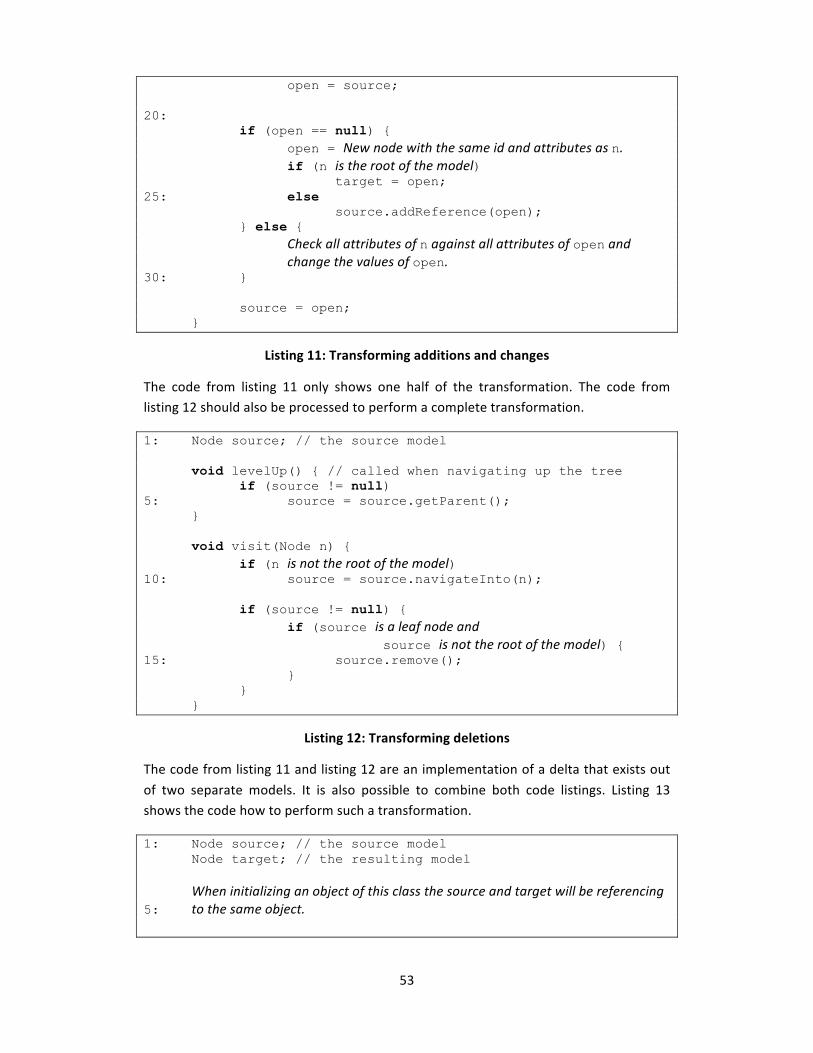
53
open = source; 20: if (open == null) { open = New node with the same id and attributes as n. if (n is the root of the model) target = open; 25: else source.addReference(open); } else { Check all attributes of n against all attributes of open and change the values of open. 30: } source = open; }
Listing 11: Transforming additions and changes
The code from listing 11 only shows one half of the transformation. The code from listing 12 should also be processed to perform a complete transformation.
1: Node source; // the source model void levelUp() { // called when navigating up the tree if (source != null) 5: source = source.getParent(); } void visit(Node n) { if (n is not the root of the model) 10: source = source.navigateInto(n); if (source != null) { if (source is a leaf node and source is not the root of the model) { 15: source.remove(); } } }
Listing 12: Transforming deletions
The code from listing 11 and listing 12 are an implementation of a delta that exists out
of two separate models. It is also possible to combine both code listings. Listing 13 shows the code how to perform such a transformation.
1: Node source; // the source model Node target; // the resulting model When initializing an object of this class the source and target will be referencing 5: to the same object.

54
void levelUp() { // called when navigating up the tree if (source != null) source = source.getParent(); 10: } void visit(Node n) { Node open=null; 15: if (n is not the root of the model) open = source.navigateInto(n); else open = source; 20: if (open == null) { open = New node with the same id and attributes as n. if (n is the root of the model) target = open; 25: else source.addReference(open); } else { if (n is set to be deleted) { // change metamodel !!! source.remove(); 30: } else { Check all attributes of n against all attributes of open and change the values of open. } } 35: source = open; }
Listing 13: Transforming additions, changes and deletions
On row 28 of listing 13 a comment is placed at the if statement. It states “change metamodel” which means that the check that will be made there, needs a change in the metamodel. The normal metamodel, in which the applications are modeled do not need
information about a transformation. The information that a node has to be deleted is only important at a model transformation. But without this extra information, a combined model transformation with additions, changes and deletions is not possible;
the changes cannot be distinguished from the deletions.
The time complexity of the proposed algorithm is worst‐case linear with respect to the number of nodes of the processed model. Because the algorithm can exist out of two passes, that both can process the whole source model, regarding only changes and
deletions, it seems that the worst‐case would be twice the number of nodes in the source model. But since deletions are the opposite of changes, both actions eliminate each other. Especially when using one single model as a delta. When using more than
one model as a delta, the tool that constructs the models of the delta should take care of multple existance of the same nodes in all models of one single delta. On the other
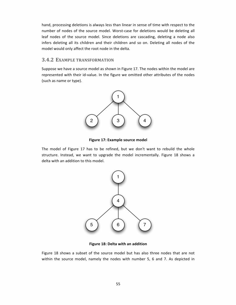
55
hand, processing deletions is always less than linear in sense of time with respect to the number of nodes of the source model. Worst‐case for deletions would be deleting all
leaf nodes of the source model. Since deletions are cascading, deleting a node also infers deleting all its children and their children and so on. Deleting all nodes of the model would only affect the root node in the delta.
3.4.2 EXAMPLE TRANSFORMATION Suppose we have a source model as shown in Figure 17. The nodes within the model are
represented with their id‐value. In the figure we omitted other attributes of the nodes (such as name or type).
Figure 17: Example source model
The model of Figure 17 has to be refined, but we don't want to rebuild the whole
structure. Instead, we want to upgrade the model incrementally. Figure 18 shows a delta with an addition to this model.
Figure 18: Delta with an addition
Figure 18 shows a subset of the source model but has also three nodes that are not within the source model, namely the nodes with number 5, 6 and 7. As depicted in
1
32 4
1
4
65 7

56
section 3.2 nodes that are in the delta but not in the source model will be added to the source model. Node 5, node 6 and node 7 are additions to the source model.
When performing a model transformation that merges the delta with the source model
our source model now looks like the model shown in Figure 18.
Figure 19: Example resulting model after the transformation
When we now use the same delta as shown in Figure 18 it will not infer an addition
again. Instead, it now will be a change or a deletion, depending on the type. Suppose it infers a change then all attributes of the nodes can be changes except the id attribute.
The source model structure stays the same but the internal values will be changed. When the delta infers a deletion then the leaf nodes will be deleted and we end up with the same model as shown in Figure 17.
The transformation algorithm will process the delta of Figure 18. When the first node
will be processed, node 1, also node 1 of the source model will be opened. After encountering that there are no changed the next node of the delta is node 4. We also open node 4 in the source model. Node 4 is also not changed so we process the next
node, node 5. When trying to open node 5 in the source model, the algorithm encounters that there is no node 5 in the source model, so we add node 5 to the source model. We do the same for node 6 and node 7 and then the whole delta is processed
and the transformation is done. We end up with the mode showed in Figure 19.
When using the same delta as shown in Figure 18 to delete nodes we start exactly as the previous transformation with opening node 1 in both the delta and the source model. Since node 1 is not a leaf node and is also the root node, we don't delete this node. Next
we open node 4 in both the delta and the source model. Also node 4 is not a leaf node so we open node 5. Node 5 also exists in the source model and node 5 is a leaf node in the delta. This means that node 5 will be deleted from the source model. The same
1
32 4
65 7
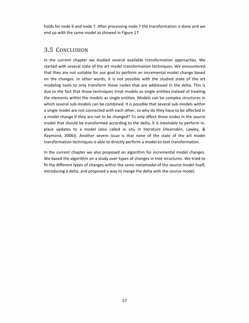
57
holds for node 6 and node 7. After processing node 7 the transformation is done and we end up with the same model as showed in Figure 17.
3.5 CONCLUSION In the current chapter we studied several available transformation approaches. We started with several state of the art model transformation techniques. We encountered that they are not suitable for our goal to perform an incremental model change based
on the changes. In other words, it is not possible with the studied state of the art modeling tools to only transform those nodes that are addressed in the delta. This is due to the fact that those techniques treat models as single entities instead of treating
the elements within the models as single entities. Models can be complex structures in which several sub‐models can be combined. It is possible that several sub‐models within a single model are not connected with each other, so why do they have to be affected in
a model change if they are not to be changed? To only affect those nodes in the source model that should be transformed according to the delta, it is inevitable to perform in‐place updates to a model (also called in situ in literature (Hearnden, Lawley, &
Raymond, 2006)). Another severe issue is that none of the state of the art model transformation techniques is able to directly perform a model‐to‐text transformation.
In the current chapter we also proposed an algorithm for incremental model changes. We based the algorithm on a study over types of changes in tree structures. We tried to
fit the different types of changes within the same metamodel of the source model itself, introducing a delta, and proposed a way to merge the delta with the source model.

58
59
4 DIFFERENT IMPLEMENTATIONS OF TRANSFORMATIONS
"At the top level, we distinguish between model‐to‐code and model‐to‐model transformation approaches. In general, we can view transforming models to code as a special case of model‐to‐model
transformations; we only need to provide a metamodel for the target programming language. However, for practical reasons of reusing existing compiler technology, code is often generated simply as text,
which is then fed into a compiler. For this reason, we distinguish between model‐to‐code transformation (which would be better described as model‐to‐text since non‐code artifacts such as XML may
be generated) and model‐to‐model transformation."
(Czarnecki & Helsen, 2003)
4.1 INTRODUCTION When implementing the proposed algorithm from the previous chapter we have several approaches to do so and also on several levels. First we have the model‐to‐model
transformation to update our working model. And second we are concerned about model‐to‐text transformations. It seems that there are differences between transformations.
Section 4.2 describes model‐to‐model transformations. This is the first step in
incremental model changing. Section 4.3 describes model‐to‐text transformations. Here we discuss several approaches of implementations and perform the actual incremental model change of applications in the file system. Section 4.4 gives the conclusion over
the research done within this chapter.
4.2 MODELTOMODEL TRANSFORMATION Since models are the primary artifacts in our development process, we start with performing a model‐to‐model transformation. The resulting model can be stored for
further use. During a transformation models are entities within the computer's memory. This means that we are not concerned with certain limitations of the platform where the changes need to happen (this will be more clear within the section of model‐to‐text

60
transformation). When performing a model transformation all nodes equal to the nodes of the delta will be looked up and changed. The number of processed nodes will be
equal to the number of nodes within the delta. This we call a fine‐grained model transformation.
4.3 MODELTOTEXT TRANSFORMATION When performing the model‐to‐text transformation we defined three approaches:
1. Entire model transformation; 2. Fine‐grained model transformation; 3. Coarse‐grained model transformation.
In the next sections we discuss the listed approaches respectively.
4.3.1 ENTIRE MODEL TRANSFORMATIONS Entire model transformation is the transformation of the complete model to files in the file system, disregarding the delta. First the model‐to‐model transformation has to be
done before a correct entire model‐to‐text transformation can be performed. This transformation can be compared with the re‐transformation (Hearnden, Lawley, & Raymond, 2006) decribe, showed in Figure 8 of chapter 2.
4.3.2 FINEGRAINED MODEL TRANSFORMATION Another way to perform a model‐to‐text transformation is the fine‐grained model
transformation. This is exactly the same as in the model‐to‐model transformation, but here we have to deal with another platform instead of the computer's memory. The model‐to‐model and model‐to‐text transformations can be performed at the same time.
As said in the previous chapter, this comes with certain limitations. The fine‐grained model transformation takes the delta as a starting point. Instead of opening nodes equal to the nodes in the delta during the transformation, entities in the file system will be
opened, such as files and folders. The number of changed elements in the file system is due to the transformation definition since the entities in the file system conform to
another metamodel than the metamodel of the models in the computer’s memory. The following figures will make the discussion more clear.

61
Figure 20: Metamodel for models in the computer’s memory
Figure 20 shows a metamodel of models that will be in the computer’s memory. The metamodel represents a structure of an application that is commonly used for data
manipulation. An overview will show multiple records of a table in a database. The columns will represent certain fields of the table. When a record is added or changed, a page will be opened where a panel with fields shows all the fields of a table of a single
record. Modules are used for separation of concerns. The construction of an overview based on a page means that the columns that are shown in the overview are based on certain fields of a panel. Panels will be responsible for tables in a database, overviews
just show multiple records of a table.
Application
Module
Page
Overview Panel
Column Field
1
*
1
*
1
*
1
*
1
*
1
*
11
1
1
part of
part of
part ofpart of
part ofpart of
based on
based on
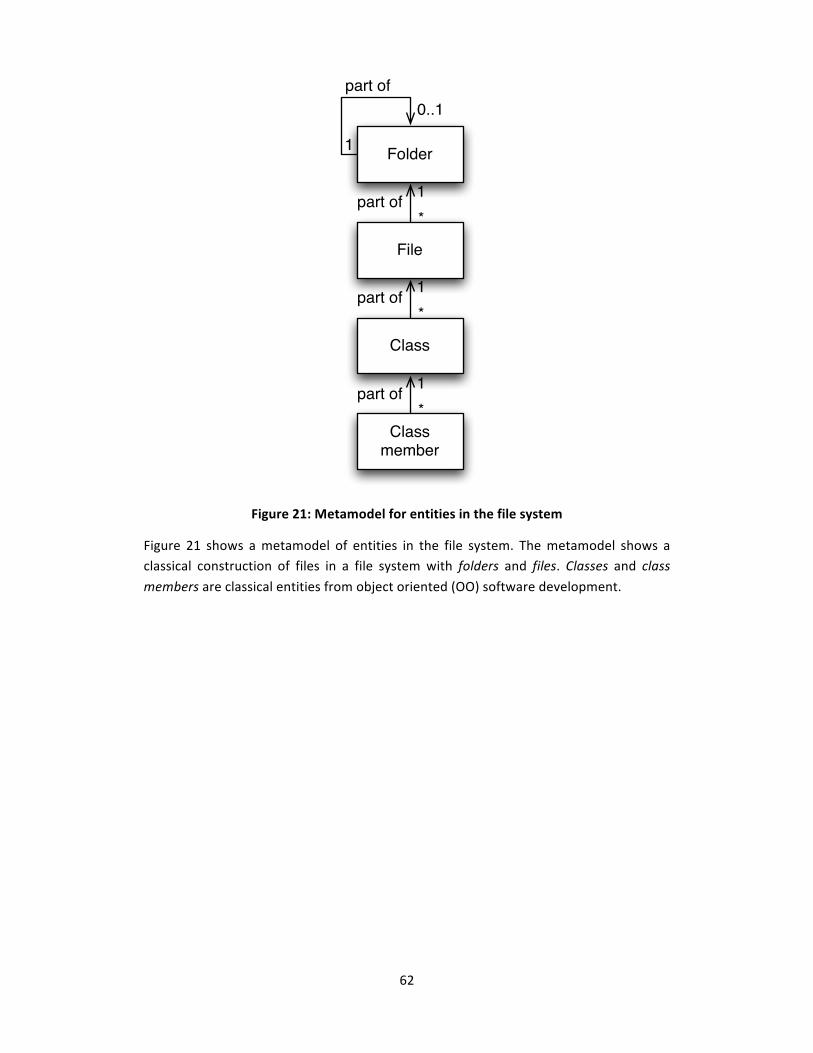
62
Figure 21: Metamodel for entities in the file system
Figure 21 shows a metamodel of entities in the file system. The metamodel shows a classical construction of files in a file system with folders and files. Classes and class
members are classical entities from object oriented (OO) software development.
Folder
File
Class
Class member
1
*part of
1
*part of
1
*part of
1
0..1
part of
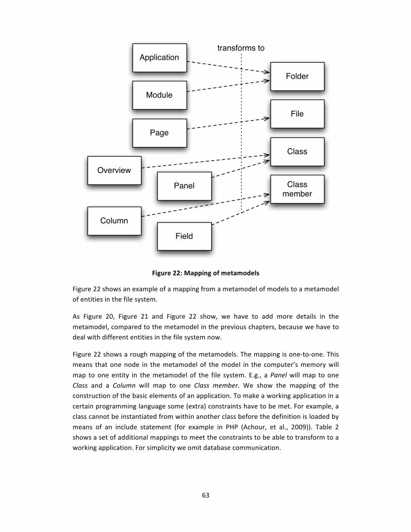
63
Figure 22: Mapping of metamodels
Figure 22 shows an example of a mapping from a metamodel of models to a metamodel of entities in the file system.
As Figure 20, Figure 21 and Figure 22 show, we have to add more details in the
metamodel, compared to the metamodel in the previous chapters, because we have to deal with different entities in the file system now.
Figure 22 shows a rough mapping of the metamodels. The mapping is one‐to‐one. This means that one node in the metamodel of the model in the computer’s memory will
map to one entity in the metamodel of the file system. E.g., a Panel will map to one Class and a Column will map to one Class member. We show the mapping of the construction of the basic elements of an application. To make a working application in a
certain programming language some (extra) constraints have to be met. For example, a class cannot be instantiated from within another class before the definition is loaded by
means of an include statement (for example in PHP (Achour, et al., 2009)). Table 2 shows a set of additional mappings to meet the constraints to be able to transform to a working application. For simplicity we omit database communication.
Application
Module
Page
Overview
Panel
Column
Field
Folder
File
Class
Class member
transforms to
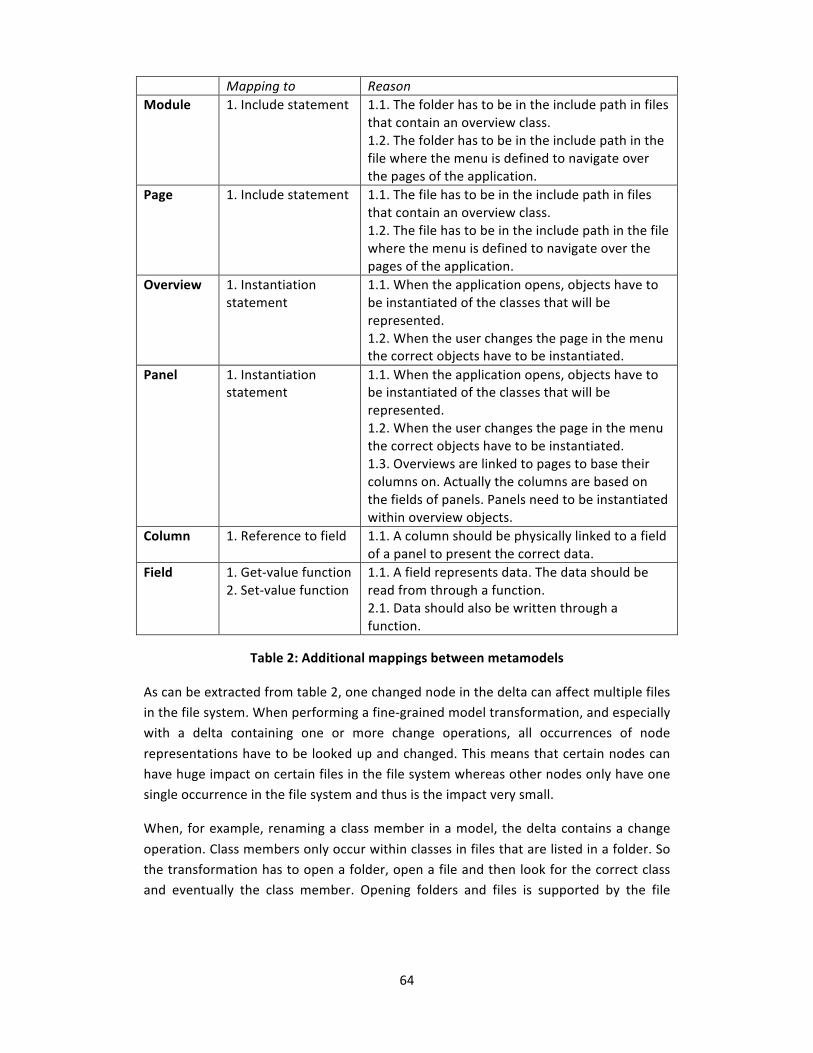
64
Mapping to Reason Module 1. Include statement 1.1. The folder has to be in the include path in files
that contain an overview class. 1.2. The folder has to be in the include path in the file where the menu is defined to navigate over the pages of the application.
Page 1. Include statement 1.1. The file has to be in the include path in files that contain an overview class. 1.2. The file has to be in the include path in the file where the menu is defined to navigate over the pages of the application.
Overview 1. Instantiation statement
1.1. When the application opens, objects have to be instantiated of the classes that will be represented. 1.2. When the user changes the page in the menu the correct objects have to be instantiated.
Panel 1. Instantiation statement
1.1. When the application opens, objects have to be instantiated of the classes that will be represented. 1.2. When the user changes the page in the menu the correct objects have to be instantiated. 1.3. Overviews are linked to pages to base their columns on. Actually the columns are based on the fields of panels. Panels need to be instantiated within overview objects.
Column 1. Reference to field 1.1. A column should be physically linked to a field of a panel to present the correct data.
Field 1. Get‐value function 2. Set‐value function
1.1. A field represents data. The data should be read from through a function. 2.1. Data should also be written through a function.
Table 2: Additional mappings between metamodels
As can be extracted from table 2, one changed node in the delta can affect multiple files in the file system. When performing a fine‐grained model transformation, and especially with a delta containing one or more change operations, all occurrences of node
representations have to be looked up and changed. This means that certain nodes can have huge impact on certain files in the file system whereas other nodes only have one single occurrence in the file system and thus is the impact very small.
When, for example, renaming a class member in a model, the delta contains a change
operation. Class members only occur within classes in files that are listed in a folder. So the transformation has to open a folder, open a file and then look for the correct class and eventually the class member. Opening folders and files is supported by the file

65
system, to look for the correct class and/or class member we have to perform a search operation within a file.
To lookup classes and class members we have to read a file. To read files we defined
two approaches: 1. Treat files as plain text; 2. Parse files.
In the first approach we read the file top‐down and try to match old occurrences of the node representation and modify them to meet the new requirements. The matching of the occurrences needs to be trivial. It could be possible that the matching algorithm
matches incorrectly when only looking at the node representation itself. In those cases it is possible to match not only on the node representation itself, but also on some more context of surrounding node representations. Since we know the previous (old) model,
we are able to reconstruct all node representations of the file we are reading. This makes the matching more precise, but is also comes with a performance penalty because we use nodes outside of the delta.
In the second approach we read the file by parsing the file. Before parsing a file, it is
obligatory to define a grammar for the entities in the file. A lexer will read the file and pass the mapped entities of the grammar to a parser that will construct an abstract syntax tree (AST) that represents the file in a structured fashion. A practical tool to
define grammars and creating a lexer and parser is ANTLR (ANother Tool for Language Recognition) (Parr, 2009). From within the AST we can do search and replace. Instead of matching textual instances, as the first approach implies, we now are able to match
objects within the AST. When a match is found, the object will be modified in the AST and after all occurrences in the file are processed, the AST can be written to a file again.
Both methods read the file completely. The advantage over the second approach in contrast to the first approach is that the second approach uses an AST. When
performing multiple changes over a single file, the AST can be left open in the memory so the file can be read only once instead of each time a node representation has to be modified. Since an AST is a tree structure and operations on trees in general are very
efficient, this is an advantage over the first approach. Another advantage is that working with an AST is less error prone, since we have to conform to a certain structure, than performing a search and replace.
4.3.3 COARSEGRAINED MODEL TRANSFORMATION A coarse‐grained model transformation is a transformation that only processes the delta
until a certain level of depth. Beyond that point the approach will transform the entities from the output model. In other words, the first part looks like the fine‐grained model transformation; nodes from the delta will be transformed. At a certain point in the
transformation the underlying nodes will not be transformed according to the delta, but

66
according to the output model. This looks more like the entire model transformation. As a consequence this approach requires the model‐to‐model transformation to be
completed before the model‐to‐text can be performed.
The coarse‐grained model transformation makes the transformation itself simpler than the fine‐grained model transformation. The transformation could be less efficient in terms of number of nodes that will be processed, but in terms of time the approach
could be more efficient because the coarse‐grained model transformation doesn't do search and replace within files. It could be possible that, for example, a delta contains changes over all entities within a file. Then the fine‐grained model transformation looks
up all entities and changes them. The coarse‐grained model transformation will, when the level of depth to stop is defined at the level of files, regenerate the complete file at once. Since the whole file has to be changed, it is easier to regenerate the whole file
again than searching and replacing all entities.
As stated above, with coarse‐grained model transformation a level of depth to stop has to be defined. In our example we used the level of files, which corresponds with the level of pages in Figure 20. This seems to be the most logical point because with the
fine‐grained model transformation also the whole file has to be read so whether the whole file will be regenerated or the whole file will be read to change seems to be the most logical point to stop the fine‐grained part of the coarse‐grained model
transformation. When defining the point at a higher level, for example, at the level of modules in Figure 20, the transformation itself will be even simpler than at the level of files, but then more files have to be generated, also files that else would not be
processed. This makes the transformation even less efficient in terms of number of nodes that will be processed.
4.3.4 SUMMARY We start the summary with an illustration, Figure 23, of the impact of the model
transformations, discussed in this chapter, to their source models. The outer ring is the complete source model. With the entire model transformation approach the smallest change will affect the whole model to be transformed (grey color). The middle circle
defines the point where the coarse‐grained model transformation stops with the fine‐grained behaviour. After that point, the coarse‐grained approach will affect all entities within this circle to be transformed with the smallest change. The inner circle defines
the smallest entity in the model. The fine‐grained approach is able to only affect those entities that actually have been changed.
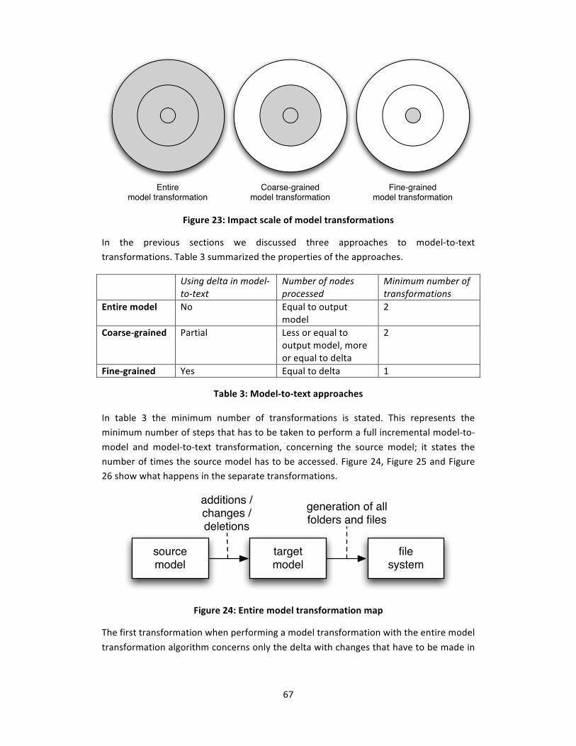
67
Figure 23: Impact scale of model transformations
In the previous sections we discussed three approaches to model‐to‐text transformations. Table 3 summarized the properties of the approaches.
Using delta in model‐to‐text
Number of nodes processed
Minimum number of transformations
Entire model No Equal to output model
2
Coarse‐grained Partial Less or equal to output model, more or equal to delta
2
Fine‐grained Yes Equal to delta 1
Table 3: Model‐to‐text approaches
In table 3 the minimum number of transformations is stated. This represents the minimum number of steps that has to be taken to perform a full incremental model‐to‐
model and model‐to‐text transformation, concerning the source model; it states the number of times the source model has to be accessed. Figure 24, Figure 25 and Figure 26 show what happens in the separate transformations.
Figure 24: Entire model transformation map
The first transformation when performing a model transformation with the entire model
transformation algorithm concerns only the delta with changes that have to be made in
Entiremodel transformation
Coarse-grainedmodel transformation
Fine-grainedmodel transformation
sourcemodel
targetmodel
filesystem
additions /changes /deletions
generation of allfolders and files

68
the source model. When generating files we need all information about all nodes of the source model because we generate the entire system. This file generation cannot be
within the same transformation step concerning the delta because in this transformation we do not affect all nodes of the source model, average case. Only worst case the whole source model will be changed but this is not likely to happen every time.
The entire model transformation does not use the delta when performing a model‐to‐
text transformation. Instead, the output model of the model‐to‐model transformation will be used. The number of nodes that will be processed is equal to the number of nodes of the output model. The minimum number of transformations is two because
first the model‐to‐model transformation has to be completed before the model‐to‐text transformation can be started.
Figure 25: Coarse‐grained model transformation map
With the coarse‐grained model transformation we still needs two separate transformations for the same reason as the entire model transformation. But here we
only concern the files that have been changed by the first transformation. Since the first transformation only concerns a part of the file, the file generation needs all information about the file so this cannot be in the same transformation. In the first transformation
we list all files that have to be generated in the second transformation so in the second transformation we can generate only those files that have been affected by the delta.
The coarse‐grained model transformation partially transforms the nodes of the output model of the model‐to‐model transformation. The coarse‐grained model transformation
also partially transforms the nodes of the delta. In fact, the transformation is a hybrid
sourcemodel
targetmodel
filesystem
additions /changes /deletions
generation of fileswithin the delta
filesystem
generation of folderswithin the delta

69
fine‐grained and entire model transformation. The number of nodes that will be processed is average case somewhere between the number of nodes of the delta and
the number of nodes of the output model. Because the transformation uses nodes from the output model, first the model‐to‐model transformation has to be completed so the minimum number of transformations is two.
Figure 26: Fine‐grained model transformation map
The fine‐grained model transformation only transforms the nodes that are present in
the delta. The number of nodes that will be processed is equal to the number of nodes within the delta. Since the model‐to‐text only transforms the nodes in the delta, the fine‐grained model transformation is able to perform the model‐to‐model and model‐
to‐text transformations at the same time, so the minimum number of transformations is one.
4.4 CONCLUSION There are two general approaches to perform a model transformation, model‐to‐model
and model‐to‐text. The most interesting one in our case is the model‐to‐text transformation because we are dependent on the limitations of the target platform, for example, the file system. Since different entities of a metamodel transform to different
entities in the file system which all could have their own limitations, further research about efficiency with respect to time in this field is needed.
In section 2.9 of chapter 2 we stated that we have two model‐dependent approaches and one semi‐model‐independent approach, as defined by (Könemann, Kindler, &
Unland, 2009). Entire model transformations and coarse‐grained model transformations are typically model‐dependent approaches. Since they both use entities of the source model that are not addressed in the delta for their model‐to‐text transformation. The
sourcemodel
targetmodel
filesystem
additions /changes /deletions
generation of folders andfiles within the delta
70
fine‐grained model transformation is semi‐model‐independent. Without optimization, it is complete model‐independent in case of a model‐to‐model transformation, since there
the entities will be matched by their unique identifier which is in both the delta and the target model the same. In our proof of concept we made an ‘optimization’ that checks whether the value has changed before actually changing it (in case of a change
operation). We put the word optimization between parentheses because it depends on the platform where the transformation is running whether an if‐statement is more efficient than an assign‐statement. In a model‐to‐text transformation we cannot
garantuee that there are the same unique identifiers in the target platform as in the delta. For example, in our proof of concept we concatenate the name‐value of a particular entity with the id‐value as a unique identifier in de target platform. Since we
know how we concatenated the unique identifier there, we also know how to reverse that step and match the retrieved id‐value against the unique identifier of the delta, but since our approach again concatenates the old name‐value and the id‐value from the
source model, we match against the complete unique identifier of the target platform. In this case we need information of the source model. This is the case for all three defined operations: additions, changes and deletions. For additions we need to know
where to add an entity, for changes we need to know what to change and for deletions we need to know what to delete.

71
5 CASE STUDY
"In mainstream practice, models, apart from the code, tend only to get sketched out, sometimes after the fact for documentation, at
varying levels of abstraction, and with largely unwritten rules used to (loosely) relate the models to themselves and to the code. This is certainly true for a typical OO development.
In a model driven approach, the vision is that models become
artifacts to be maintained along with the code. This will only happen if the benefit obtained from producing the models is considerably more and the effort required to keep them in line with the code is
considerably less than current practice. Models are valuable as tools for abstraction, for summarizing, and for providing alternative perspectives. The value is greatly enhanced if models become
tangible artifacts that can be simulated, transformed, checked etc., and if the burden of keeping them in step with each other and the delivered system is considerably reduced.
Tooling is essential to maximize the benefits of having models, and to
minimize the effort required to maintain them. Specifically, more sophisticated tools are required than those in common use today, which are in many cases just model editors. What might these tools
be?"
(Kent, 2002)
5.1 INTRODUCTION As a case study to support our research we make use of a tool developed by the company Novulo in the Netherlands (Novulo, 2009). The tool Novulo created is called
the Novulo Architect. Within the Novulo Architect it is possible to create models of business applications containing a database. It is also possible to store business logic and workflow management in the model. These models can be transformed into source
code files of a particular language. In this way the Novulo Architect generates direct working applications for the end‐user.

72
The issue of retransforming all files again is also present at Novulo. The Novulo Architect is able to change existing models but instead of generating only those files that are
affected by a change, it transforms the whole model again to source code files. This is an expensive operation in matters of time because models can get very large but changes are usually very small. We will see in this chapter that usually the higher the number of
revisions of a model, the smaller the set of changes.
This chapter studies different applications developed with the Novulo Architect and the changes that are performed onto the different models. With this empirical research, we are able to construct meaningful test models which we use in chapter 6 to benchmark
our model transformation algorithms against each other.
5.2 NOVULO ARCHITECT The Novulo Architect is a development platform in which applications can be built in a top‐down approach. First pages and elements can be added to a model from which the
database will be extracted. After creating pages and elements expressions can be defined to add business logic to the application. For example, to show or hide elements, make calculations or define data filters. Furthermore workflows can be defined to
model processes that have to be invoked when pressing a button, for example, by an end‐user. As an extra feature all elements modeled within the Novulo Architect can be marked as custom. This means that when the model will be transformed to a target
platform, for example, an implementation in a lower‐level language, the elements marked as custom will be generated in separate folders to be implemented manually by a programmer in the target language. The files are generated in separate folders to
ensure that the files will not be overwritten the next time the model will be transformed. Custom elements are treated as black boxes; the input and output are known the Novulo Architect. Figure 27 shows a screenshot of the Novulo Architect.

73
Figure 27: Screenshot of the Novulo Architect
5.2.1 METAMODEL / DOMAIN SPECIFIC LANGUAGE
The Novulo Architect in fact is a metamodel or DSL for database driven applications. Novulo tries to be as generic as possible to support the modeling of complete
applications. Within the metamodel of Novulo we find four distinct modeling branches.
In the first branch the page structure is stored. Here the layout of the application is modeled with all references to each other. With this, the user is able to navigate through the application after it is generated.
The second branch is the database layer. This branch is dependent on the first branch
because of the top‐down approach. This means that the database is derived from the pages created. A developer is able to change the attributes of the database branch without corrupting the application.
The third branch is the business logic. Usually customers do not want flat data in their
applications. They rather want filtered, sorted data which they can use in their daily work. Also elements that are not needed in some situations should not be visible to the user and for reporting some support for making functions and calculations would come
handy. Novulo created an own expression language that is able to query all data on the basis of the model. With this it is possible to make constraints in the model which only take effect in the actual generated application (on a lower level). This constraints can be
filters and sorts on data overviews, conditional visibility of elements in the application, conditional editibility of elements, default values for elements, calculations over sets of data and many more.

74
The fourth branch is the workflow management. This is used for interaction. When certain events happen in the application, for example, a button is clicked or a page is
loaded, certain behaviour can be defined in the Novulo Architect. This way the developer is able to force the end‐user to work with the application in a pre‐defined manner. The developer can put constraints to interactions of the end‐user and force
actions to take place at a certain point in the application. A developer is able to direct the behaviour of events in the application.
An extra feature of the Novulo Architect is that in every branch, the developer is able to mark elements as custom. This means that the element will turn into a black box for the
Novulo Architect. The input and output for the black box can be defined, but the actual implementation of the black box in the lower code level is not known. In other words, the standard code generation for that part is probably not sufficient in a certain
situation so the developer can decide to make its own implementation there. This gives the developer a huge control over the actual generated application without corrupting the model. In code generation the part that was marked custom will be generated only
once because else the black box implementation could be overwritten by a new code generation. This black box functionality is also called model based development (MBD), which is a trademark of the OMG, because the model is only used once to create the
black box and the implementation is to be done by the developer itself.
5.2.2 CODE GENERATION The Novulo Architect uses the entire model transformation approach to generate code. Each time a model is stored code generation can take place, this is up to the developer to perform it whether or not.
All files and folders will be generated and in the end an external program will check for
each file wheter or not there is a change in contents of the just generated files and the files in the repository of the external program. If the program encounters a change in a
file, the newly generated file will be added to the code repository. All other files from which the contents are not changed in comparison to the files already in the repository will be discarded. This causes a lot of overhead and uses a lot of time.
5.3 APPLICATIONS With the Novulo Architect, around 250 projects are developed. This section describes
several distinct applications that are created within the Novulo Architect. Per application we give the number of revisions the application went through, the number of developers, which may relate to the number of revisions and an overview of the
impact of changes between the revisions. We studied the types of changes and the relation with the changes and the revision of the model.

75
We start this section with an overview of all revisions and number of nodes in a graph, Figure 28. In the next subsections we give some more background information about
the data in the graph.
Figure 28: Distribution of model revisions against number of nodes
5.3.1 SMALL CRM SYSTEM We start with a small CRM system. This system was used to contain a huge amount of data about possible customers. The system itself was very small and simple and was
only needed to keep track of the information communicated with the relations in a organized way.
The project took 2 days to complete. Only one programmer (modeler) worked on the application and in the end the number of revisions was 39. In other words, 39 times a
delta changed the model. Since it is not obligatory to generate code with each revision, the number of times the whole model was generated to the file system could be less. The transformation of the 39th revision took about 8 seconds.
The total number of nodes in the model was 13558. When we look at Figure 28 we can
see that it is not very much compared to the other applications. The history of the different deltas according to Figure 28 are not very spectacular. We see that in the first 5 revisions the base of the application was made. After that the number of nodes stayed
steady for a while, meaning changes over the model or just re‐generation of files. In
0
10000
20000
30000
40000
50000
60000
70000
80000
90000
100000
1 12
23
34
45
56
67
78
89
100
111
122
133
144
155
166
Nr of nod
es
Revisions
Vacancy system
Migrauon tool
Small CRM

76
later revisions some extra functionality was added which caused the number of nodes to rise. The last few revisions were only changes or re‐generations.
5.3.2 VACANCY SYSTEM The vacancy system was a more complicated application than the small CRM system.
Within this application the vacancies with applications of relations was to be managed. This contained some complex data constructions so there were a lot of revisions that changed the application.
The project took about 5 months to complete. Two programmers worked on the
application. The transformation of the 173th revision took 34 seconds. The cumulative time of all model‐to‐model and all model‐to‐text transformations is more than 1,5 hours in total, supposing that with every revision file generation was performed.
The total number of nodes for the vacancy system was 52453. In the first 50 revisions a
lot of functionality was added to the application, after that some functionality was deleted causing a decreased number of nodes. Then a lot of small things were added, some deleted, but in the number of additions and deletions seemed to be smaller and
smaller. We cannot say anything about the changes because it cannot be seen when only looking at the number of nodes of the resulting model.
5.3.3 DATABASE MIGRATION TOOL
The database migration tool was used to migrate data of multiple accounts of a financial system into one application. The project was very straightforward so very few revisions
are made. Also the time spent to complete the application was very little.
The project took about 2 weeks to complete. Only one programmer worked on the application. The transformation time of the 38th revision took about 26 seconds.
The total number of nodes for the database migration tool was 84560, the biggest application we included in the comparison. In the first 15 revisions a very high number
of additions were done. Around revision 30 again a lot of additions were done. In the end again the number of additions and deletions was getting smaller and smaller.
5.4 CONCLUSION When we look at the graph of Figure 28 we can conclude that in the applications we
looked at, the number of additions and deletions in the end were very low. It is assumed that the number of changes was also getting smaller and smaller due to the fact the application was getting finished, so huge changes are unlikely to happen at that stage.
77
6 BENCHMARKING THE IMPLEMENTATIONS
“Benchmarking is the process of comparing the cost, cycle time, productivity, or quality of a specific process or method to another
that is widely considered to be an industry standard or best practice. Essentially, benchmarking provides a snapshot of the performance of your business and helps you understand where you are in relation to
a particular standard (Dumford, 2009). The result is often a business case for making changes in order to make improvements. The term benchmarking was first used by cobblers to measure ones feet for
shoes. They would place the foot on a "bench" and mark to make the pattern for the shoes. Benchmarking is most used to measure performance using a specific indicator (cost per unit of measure,
productivity per unit of measure, cycle time of x per unit of measure or defects per unit of measure) resulting in a metric of performance that is then compared to others.”
(Wikipedia, 2009)
6.1 INTRODUCTION This chapter we discuss the timing results of the benchmarks of the model transformation approaches over certain base models. To perform the benchmarks we developed a proof of concept. This chapter also discusses what kinds of benchmarks we
perform and how they are constructed. In the end we come up with a conclusion of which model transformation approach is the most efficient in general.
6.2 TRANSFORMATIONS In this section the actual benchmarking will be performed and discussed.
All benchmarks are performed on an Apple MacBook with 2.16 GHz Intel Core 2 Duo
processor, 2 GB 667 MHz DDR2 SDRAM memory and running Mac OS X version 10.5.7. The Java version used was 1.6.0_07. For the virtual machine the argument –Xmx1024m was used to allocate 1024 MB of memory.

78
6.2.1 BASE MODELS To make good estimations about the proposed model transformation approach of chapter 3 and chapter 4, we define a set of base models on which we will perform certain benchmarks. To start with benchmarking we first have to define what we want
to benchmark. We are interested in the best implementation for the different deltas and base models. The other interesting part is the effect on the different platforms and entities within the platforms. For example, when performing a model‐to‐model
transformation all transformations happen in the computer's memory, but when performing a model‐to‐text transformation, the transformations will happen in the file system. Within the file system the different entities have different properties. We are
interested in which type of transformation is most suitable for different types of transformations on different levels of entities (in the file system).
As shown in Figure 21, we defined four different entities in the file system: • Folders;
• Files; • Classes; • Class members.
Table 4 shows the different entities in the file system against several crucial properties.
Physical entity Part of other entity Need to be read Folder Yes No No File Yes No Yes Class No Yes, file Yes Class member No Yes, file Yes
Table 4: Properties of entities in the file system
As shown in table 4, classes and class members share the same properties; they can be
treated the same. The applications to which we transform need to contain at least folders, files and classes. Because we identified three different entities in the file system we want to use in our benchmarks, we also need the corresponding entities in the
models. According to Figure 22 our minimum application needs at least a module, a page and a panel (or an overview).
6.2.2 PROOF OF CONCEPT To benchmark the approach we proposed, we developed a proof of concept (POC) application. Within the POC we implemented the complete metamodel of Figure 20.
Also the mapping of Figure 22 is implemented so the POC is able to transform to the correct entities in the file system according to the metamodel of Figure 21.
79
The POC is a command line tool written in Java that returns timing values over a certain model transformation.
6.2.3 GENERAL REMARKS For the benchmarking we picked out a subset of the available entities of the metamodel
of Figure 20. Next to the minimum set of entities as discussed in the previous section we also included the field entity to give a more representative benchmark because the file gets more complex; when looking for a field entity we first have to search and open the
correct class.
Since we included fields in the benchmarking, the number of panels can be reduced to only one. The single panel will contain all fields. The algorithm does not know there is only one panel so it still has to search.
Since folders imply only more files in the file system, we reduce the number of modules
also to only one. This single module will contain all pages. The algorithm still has to open the module and folder in the file system so there is no difference in increasing the number of modules and pages or only pages and keep the number of modules one.
We used two types of base models. For the additions we used empty base models
consisting only of one node namely the application node. For changes and deletions we used base models of 25 pages with each 25 fields. That means a total of 25 times 25 is 625 fields. Because there are 25 pages there are also 25 panels, so we have to add 50 to
the 625. We also have to add 3 entities to the 675 because of the application node, the module and the panel. So the total number of entities was 678. This is not much in comparison to the models of the case study of chapter 5, but the most deltas are likely
to be very small. If a delta affecting only 5 files will be transformed in a model with a total of 500 files, the impact of the coarse‐grained and fine‐grained model transformations will be too small in comparison to the entire model generation. We
want to give a clear view in the benchmarks so we keep the size of the base models small and also the deltas will be small. If we use larger base models we also need larger
deltas which give exactly the same results only with a different offset; the graph will look the same only the numbers change.
To make representative statistical benchmarks we need to repeat the same experiment several times. We decided to repeat each experiment 1000 times, to let the Java virtual
machine allocate enough memory we first run 10 repetitions of the same experiment which we do not include in the benchmark. So in fact we run 1010 experiments. The next graph shows the distribution of timing results over 1000 measurements of an
experiment of changing 1 field in 1 page in a system consisting of 1 page containing 25 fields.

80
The following numbers also hold for the total distribution: • Median: 0.649 ms
• Mean: 2.133 ms • Standard deviation: 4.917 ms
Figure 29: Total distribution of timings of 1000 experiments
Figure 29 shows the total distribution of 1000 experiments of 1 benchmark.
If we reduce the results by cutting off all measurements outside the range of twice the
standard deviation on top of the mean we get the graph of Figure 30.
0
50
100
150
200
250
0.0
3.6
7.2
10.8
14.4
18.0
21.6
25.2
28.8
32.4
36.0
39.6
43.2
46.8
50.4
54.0
57.6
61.2
64.8
68.4
72.0
75.6
79.2
82.8
86.4
90.0
93.6
Freq
uency
Time (ms)

81
Figure 30: Trimmed distribution of timings of 1000 experiments
The following numbers hold for the trimmed distribution: • Median: 0.635 ms
• Mean: 1.794 ms
The results of the graph of Figure 30 by cutting off all extraordinary measurements gives us a more representative view. This new set comes with a new trimmed mean and trimmed median. For the benchmarks we use the median of the trimmed distribution.
6.2.4 ADDITIONS BENCHMARKS Base Pages
Base Fields
Delta Pages
Delta Fields
Entire (ms)
Coarse (ms)
Fine (ms)
Benchmark 1 0 0 5 25 2.55 2.1285 3.754 Benchmark 2 0 0 10 25 5.008 4.377 8.204 Benchmark 3 0 0 15 25 7.646 7.105 12.522 Benchmark 4 0 0 20 25 10.015 9.466 16.2155 Benchmark 5 0 0 25 25 13.233 12.478 20.99 Benchmark 6 0 0 1 5 0.8555 0.538 0.6905 Benchmark 7 0 0 1 10 0.903 0.56 0.814 Benchmark 8 0 0 1 15 0.935 0.601 0.867 Benchmark 9 0 0 1 20 0.977 0.655 0.938 Benchmark 10 0 0 1 25 1.036 0.67 1.092
Table 5: Addition benchmarks
0
50
100
150
200
250
0.0
0.5
1.0
1.5
2.0
2.5
3.0
3.5
4.0
4.5
5.0
5.5
6.0
6.5
7.0
7.5
8.0
8.5
9.0
9.5
10.0
10.5
11.0
11.5
Freq
uency
Time (ms)

82
Table 5 shows the timing results of 30 different experiments. All experiments add nodes to an empty model (0 pages with 0 fields). In the following figures we collected those
timing results in graphs.
Figure 31: Benchmarks 1 to 5: nr of pages vs. time
In Figure 31 we can easily see that when enlarging the delta, the transformation time
will expand. We notice that the coarse‐grained and the entire model transformation expand with the same linear value, but the fine‐grained model transformation expands with a larger amount, meaning that it is very inefficient in comparison to the other
approaches, regardless the linear growth of the fine‐grained model transformation time. We conclude here that the coarse‐grained model transformation is the most efficient with this types of model transformations.
0
5
10
15
20
25
5 10 15 20 25
Time (m
s)
Nr of pages
Enure
Coarse
Fine
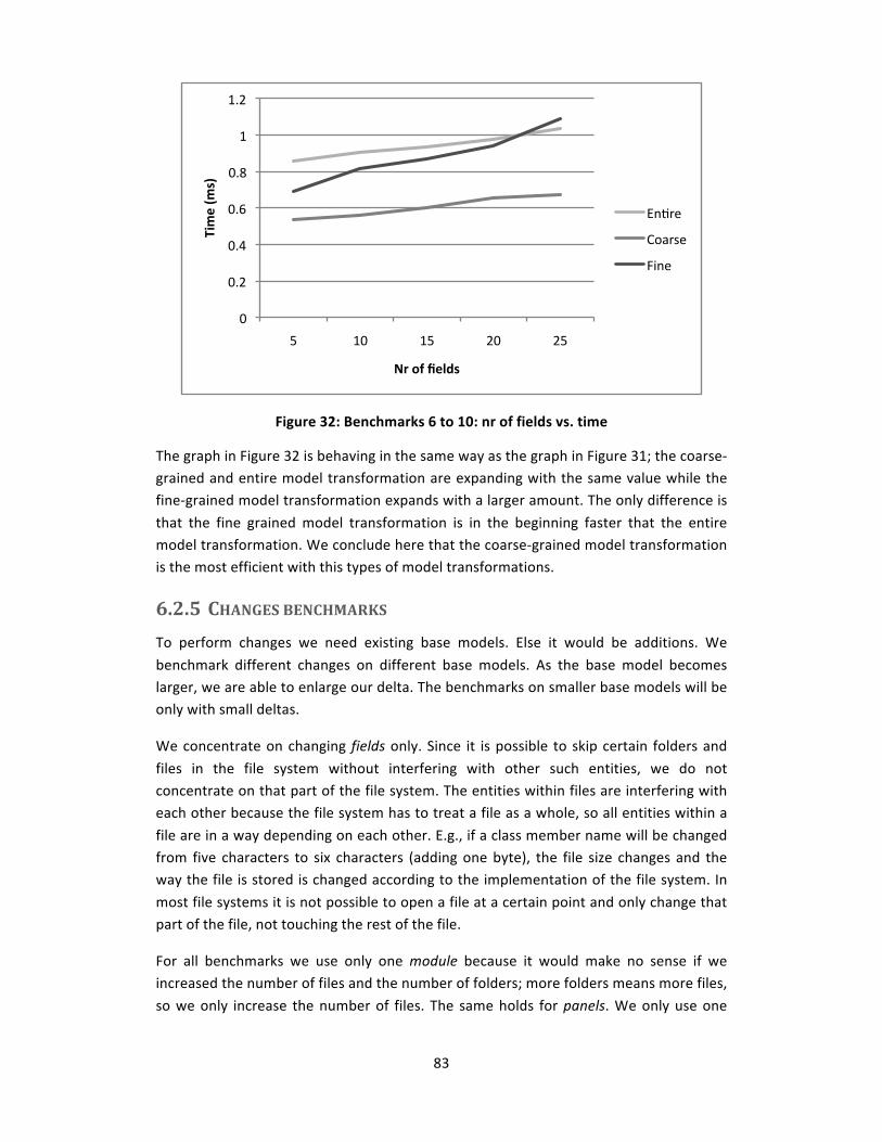
83
Figure 32: Benchmarks 6 to 10: nr of fields vs. time
The graph in Figure 32 is behaving in the same way as the graph in Figure 31; the coarse‐grained and entire model transformation are expanding with the same value while the fine‐grained model transformation expands with a larger amount. The only difference is
that the fine grained model transformation is in the beginning faster that the entire model transformation. We conclude here that the coarse‐grained model transformation is the most efficient with this types of model transformations.
6.2.5 CHANGES BENCHMARKS To perform changes we need existing base models. Else it would be additions. We
benchmark different changes on different base models. As the base model becomes larger, we are able to enlarge our delta. The benchmarks on smaller base models will be only with small deltas.
We concentrate on changing fields only. Since it is possible to skip certain folders and
files in the file system without interfering with other such entities, we do not concentrate on that part of the file system. The entities within files are interfering with each other because the file system has to treat a file as a whole, so all entities within a
file are in a way depending on each other. E.g., if a class member name will be changed from five characters to six characters (adding one byte), the file size changes and the way the file is stored is changed according to the implementation of the file system. In
most file systems it is not possible to open a file at a certain point and only change that part of the file, not touching the rest of the file.
For all benchmarks we use only one module because it would make no sense if we increased the number of files and the number of folders; more folders means more files,
so we only increase the number of files. The same holds for panels. We only use one
0
0.2
0.4
0.6
0.8
1
1.2
5 10 15 20 25
Time (m
s)
Nr of fields
Enure
Coarse
Fine
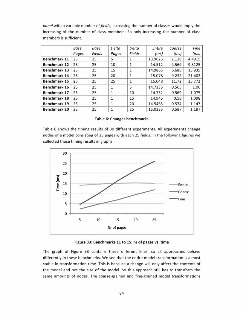
84
panel with a variable number of fields; increasing the number of classes would imply the increasing of the number of class members. So only increasing the number of class
members is sufficient.
Base Pages
Base Fields
Delta Pages
Delta Fields
Entire (ms)
Coarse (ms)
Fine (ms)
Benchmark 11 25 25 5 1 13.9625 2.128 4.4915 Benchmark 12 25 25 10 1 14.512 4.569 9.8125 Benchmark 13 25 25 15 1 14.9865 6.688 15.935 Benchmark 14 25 25 20 1 15.078 9.232 21.402 Benchmark 15 25 25 25 1 15.048 11.72 25.772 Benchmark 16 25 25 1 5 14.7235 0.565 1.06 Benchmark 17 25 25 1 10 14.732 0.569 1.075 Benchmark 18 25 25 1 15 14.945 0.58 1.098 Benchmark 19 25 25 1 20 14.5465 0.574 1.147 Benchmark 20 25 25 1 25 15.0235 0.587 1.187
Table 6: Changes benchmarks
Table 6 shows the timing results of 30 different experiments. All experiments change nodes of a model consisting of 25 pages with each 25 fields. In the following figures we
collected those timing results in graphs.
Figure 33: Benchmarks 11 to 15: nr of pages vs. time
The graph of Figure 33 contains three different lines, so all approaches behave
differently in these benchmarks. We see that the entire model transformation is almost stable in transformation time. This is because a change will only affect the contents of the model and not the size of the model. So this approach still has to transform the
same amounts of nodes. The coarse‐grained and fine‐grained model transformations
0
5
10
15
20
25
30
5 10 15 20 25
Time (m
s)
Nr of pages
Enure
Coarse
Fine

85
show an expanding amount of time. This is because the number of entities that are changed is increased and also the number of files is increased. We conclude here that
the coarse‐grained model transformation is the most efficient with this types of model transformations.
Figure 34: Benchmarks 16 to 20: nr of fields vs. time
The graph of Figure 34 shows slightly increasing fine‐grained values. This is because more entities in the file have to be searched and replaced. For the coarse‐grained and entire model transformation timing results stay the same because they both have to
transform the same amount of pages into files. We conclude here that the coarse‐grained model transformation is the most efficient with this types of model transformations.
6.2.6 DELETIONS BENCHMARKS Base Pages
Base Fields
Delta Pages
Delta Fields
Entire (ms)
Coarse (ms)
Fine (ms)
Benchmark 21 25 25 5 0 11.847 0.621 0.678 Benchmark 22 25 25 10 0 10.736 1.073 1.215 Benchmark 23 25 25 15 0 6.788 1.52 1.79 Benchmark 24 25 25 20 0 5.823 2.654 2.946 Benchmark 25 25 25 25 0 3.617 3.3045 3.48 Benchmark 26 25 25 1 5 15.1075 0.62 1.028 Benchmark 27 25 25 1 10 14.9355 0.6325 0.9925 Benchmark 28 25 25 1 15 14.682 0.641 0.9345 Benchmark 29 25 25 1 20 14.921 0.636 0.82 Benchmark 30 25 25 1 25 14.972 0.617 0.7505
Table 7: Deletions benchmarks
0
2
4
6
8
10
12
14
16
5 10 15 20 25
Time (m
s)
Nr of fields
Enure
Coarse
Fine
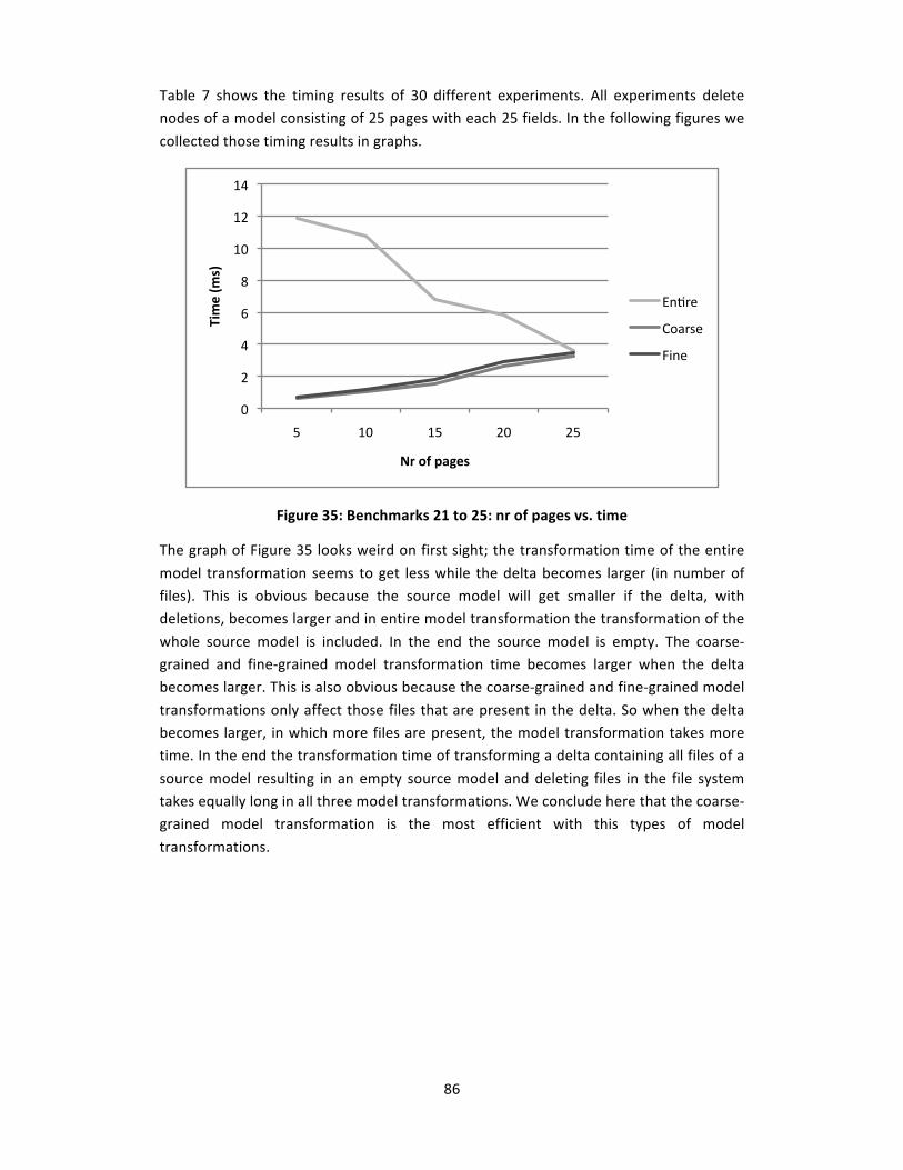
86
Table 7 shows the timing results of 30 different experiments. All experiments delete nodes of a model consisting of 25 pages with each 25 fields. In the following figures we
collected those timing results in graphs.
Figure 35: Benchmarks 21 to 25: nr of pages vs. time
The graph of Figure 35 looks weird on first sight; the transformation time of the entire
model transformation seems to get less while the delta becomes larger (in number of files). This is obvious because the source model will get smaller if the delta, with deletions, becomes larger and in entire model transformation the transformation of the
whole source model is included. In the end the source model is empty. The coarse‐grained and fine‐grained model transformation time becomes larger when the delta becomes larger. This is also obvious because the coarse‐grained and fine‐grained model
transformations only affect those files that are present in the delta. So when the delta becomes larger, in which more files are present, the model transformation takes more time. In the end the transformation time of transforming a delta containing all files of a
source model resulting in an empty source model and deleting files in the file system takes equally long in all three model transformations. We conclude here that the coarse‐grained model transformation is the most efficient with this types of model
transformations.
0
2
4
6
8
10
12
14
5 10 15 20 25
Time (m
s)
Nr of pages
Enure
Coarse
Fine

87
Figure 36: Benchmarks 26 to 30: nr of fields vs. time
The graph of Figure 36: Benchmarks 26 to 30 looks almost stable in time for all sizes of delta. The size of the delta in comparison to the source model is 1 in 25, so that declares why the entire model transformation does not show significant differences. In fact, the
source model is getting smaller and smaller so the transformation time shrinks. But since file handling is an expensive operation it is not very visible in the graph. For the coarse‐grained model transformation we see that the transformation time increases in
the first four deltas. The last delta is faster again. This is also because of the slight difference in the change in the file. In coarse‐grained model transformation still complete files are handled so the slight different in file size does not make significant
changes in transformation time. For the fine‐grained model transformation we see that there is a significant transformation time change with the different sizes of delta. This is because all single operations are quite expensive in time with this approach. We see
that when enlarging the delta, resulting in smaller files, the transformation time shrinks with around 25 percent. We conclude here that the coarse‐grained model transformation is the most efficient with this types of model transformations.
6.3 CONCLUSION We can conclude over this chapter that the coarse‐grained model transformation is the most efficient approach over all different types of (straightforward) deltas. With additions to a model, changes over a model and deletions of elements of a model the
coarse‐grained model transformation is the fastest approach. We did not take into account changes that affect the complete source model. Worst case such changes will cause transformations that are to be compared to entire model transformation, since
the coarse‐grained model transformation approach uses the same file generation
0
2
4
6
8
10
12
14
16
5 10 15 20 25
Time (m
s)
Nr of fields
Enure
Coarse
Fine
88
approach as the entire model transformation approach. The only difference is that the number of files is reduced in the coarse‐grained approach (when having a delta that not
affects the whole model).
The reason why the coarse‐grained model transformation is the fastest is because it does not have the overhead of transforming more pages than affected in the delta, in contrast to the entire model transformation, and it also does not have the overhead of
parsing files in contrast to the fine‐grained model transformation. As can be concluded from this chapter there is no trade‐off between the coarse‐grained and the fine‐grained model transformation. In our examples the coarse‐grained approach performs in all
cases better than the fine‐grained approach.
89
7 CONCLUSIONS
This chapter concludes the thesis. Here we will summarize our
findings of the previous chapters and give an impression of a metamodeling approach to incremental model changes.
7.1 SUMMARY In this section we briefly summarize the contents of the previous chapters.
Chapter 2 described the background information about the subject of MDE. We
discussed a number of state of the art model transformation techniques. We also studied the concept of incremental development. We introduced here already two approaches of incremental development with models which we discussed in chapter 4.
In chapter 3 we covered several approaches to perform incremental model changes in
model‐to‐model fashion. We found that there are three different operations possible on models, as data structures. We defined additions, changes and deletions. Those three operations are the basic operations for manipulations of data structures. We refer to set
of those operations that will be used in a transformation as delta. We implemented the operations in three state of the art model driven transformation techniques, respectively, QVT Relations, QVT Operational Mappings and ATL. We were able to
perform the three operations in all three techniques, but it turned out that in none of the techniques we are able to perform a real incremental model change where a
transformation only affected the minimum set of entities described by the delta; all three approaches affected the whole source model. Because of the negative results of the state of the art model transformation techniques we presented our own proposal to
perform such a model transformation, where the nodes of the source model that are affected by a change are addressed in the delta. We implemented our approach in a traditional imperative language (Java).
In chapter 4 we discussed three approaches to implement a model‐to‐text
transformation with the use of our own proposal of chapter 3. The three approaches are an entire model transformation, a coarse‐grained model transformation and a fine‐grained model transformation. In the entire model transformation the whole source
model will be affected. So if a delta only changes one single entity in the source model, all other entities also will be affected. Another approach is to only affect the node in the source model that has been addressed in a delta containing one entity. We call this fine‐
grained model transformation since the granularity is the finest possible. In coarse‐
90
grained model transformation we define a point in the model where we will stop getting deeper in the model. The point we defined is the level where entities in the model
become files in the file system. When an entity is changes below that point, all entities will be affected started with the entity where we stopped. With a model‐to‐model transformation we are always able to perform a fine‐grained model transformation
since all entities are treated the same in the computer’s memory. In a model‐to‐text transformation we encounter the limitations of the target platform: the file system. We discussed the three different approaches to be able to benchmark the different
approaches in chapter 6. So after, or during, a real incremental model‐to‐model transformation we perform a model‐to‐text transformation to keep the model (files and folders) in the file system also synchronized.
In chapter 5 we addressed a commercial product, the Novulo Architect, which copes in a
way with the problems we address in this thesis. It performs in‐place updates on the source model, but when performing a model‐to‐text transformation the whole source model is to be transformed, instead of only transforming the differences since the last
model‐to‐text transformation. We used several applications which are developed with this product as a case study for the change impact scenarios.
Chapter 6 discussed the three different model‐to‐text approaches in the sense of benchmarking. We defined several source models and deltas and performed the
transformations of which we collected the time the transformation took. We presented those timing results in graphs so we visualized the benchmarking. It turned out that the fine‐grained approach, where the nodes affected are all addressed in the delta, is not
that efficient in model‐to‐text than in model‐to‐model transformations.
7.2 RESEARCH QUESTIONS We are now able to answer our research questions.
RQ1: Which files have to be synchronized when a model is changed and is it possible to only affect those files?
When changing a source model we are able to model the changes themselves in the
same metamodel as the source model. We know at which point in the metamodel entities will become file, we are able to identify the files that have to be synchronized. When performing a transformation to synchronize files it depends on the
transformation approach what information we need to synchronize. When, for example, using the fine‐grained model transformation, we only need the information that is already in the delta. The correct file can be found, the item to change can be found and
the synchronization step can be performed. When using the coarse‐grained model transformation, we need, apart from the information in the delta, also information about the rest of the file from the source model to reconstruct the file (since in the
91
coarse‐grained model transformation files will be replaced). When a model uses references to other parts of the model, also those files have to be synchronized when a
change takes place that is used in multiple files. So it is possible to only affect those files that are addressed in the delta. Only when using the entire model transformation approach all files will be affected.
RQ2: If specific file generation is possible, how to perform such a transformation?
As stated with the answer of research question 1, with the coarse‐grained and fine‐
grained model transformation approaches we are able to perform specific file generation. Whereas the coarse‐grained approach actually re‐generates the affected files of the delta, the fine‐grained approach will leave the file intact but only changes a
part of the file, so no re‐generation.
RQ3: Which transformation method performs better for various source models and changes to the model?
As researched in chapter 6, the coarse‐grained model transformation approach performs best on all different models and various deltas. Whereas the entire model
transformation approach has the overhead of re‐generating all files, also those that are not affected by a change and the fine‐grained approach has the overhead of parsing files, the coarse‐grained model transformation approach uses best of both methods. Re‐
generating files is not a bad idea because with the fine‐grained approach we still are handling complete files (after parsing the code we need to generate code again to store the changed file again). Though with the fine‐grained approach we are able to just affect
those files that are affected by a change in the model and leave the other files ontouched. We combined the specific file processing of the fine‐grained model
transformation approach with the file re‐generation of the entire model transformation approach to get the best results. The limitation of the fine‐grained approach where files have to be parsed completely is due to the file system. When a file system is able to
perform efficient file changes, maybe the fine‐grained model transformation approach will be best performing.
7.3 GENERALIZATION The problem we are addressing in this thesis is mainly a synchronization problem. When there are more than one separate instantiations of a model representing the same
entity, the need for synchronization occurs when one of the models is changed apart from the other(s). There are several ways to cope with this problem. Hearnden et al. (Hearnden, Lawley, & Raymond, 2006) proposed ways to perform synchronization
transformations. Also Könemann et al. (Könemann, Kindler, & Unland, 2009) did research in this are and in our thesis we also propose several solutions. The commonality in those approaches is that they all use a delta to perform their

92
transformations. A delta is the exact difference between two different versions of a model. The way in which the delta is represented and constructed is different. For
example, Könemann constructs the delta by performing static analysis on two consecutive versions of a model. In our case we only have one single version and record the operations that are performed on that model in our delta. Könemann also
represents the delta in a general structure (metamodel), this enables them to use the delta also for different purposes, besides synchronizing a model with the same structure. In our case the delta conforms to the same metamodel as the source model.
Since the source model will be refined with the delta and also conforms to the same metamodel, this is no difference with the approach of Könemann. But when we want to synchronize, for example, the files in the file system, we need to have a mapping of the
metamodel of the source model to the entities within the file system. When the hierarchy in the file system differs from the hierarchy of the model, synchronizing the model could get very complex if not impossible. Further research should turn out if this
is feasible.
The approach we used in this thesis for our examples and benchmarking are very straightforward to get the results in the most optimal environment. For example, when a model has very much dependencies, it could happen that only one single change in
one entity affects more entities than only itself. Worst case it could affect the whole model. The way we represent our delta is also capable of dealing with this problem in an efficient way. When, for example, an entity has a lot of references to other entities and
also a lot of entities referencing to it, we are able to construct a dependency graph when changing that particular entity. It depends on the implementation of the tool that
constructs the delta, but it would be very efficient if every entity that is referred from another entity keeps track of those references (back references). This way we can easily construct a dependency graph to see which other entities must also be within the delta
to be changed. When the delta is complete, the transformation handles the sychronization with the file system. So this way a single change of one entity can cause multiple files to be changed. Worst case all files.
In coarse‐grained model transformation we defined the granularity to stop at the level
of files. It depends on the mapping of the metamodel to the file system how efficient this transformation will be. A higher granularity at file level means a higher granularity possible in coarse‐grained model transformation. When the granularity is increased, the
effect probably is that files also become smaller, so less code has to be generated. This also means that less time is needed to generate those files. The granularity ‘chosen’ for the coarse‐grained model transformation depends on the type of changes. A change
could also mean that multiple files are affected so when implementing our approach a study has to be done of which changes are most likely to happen to optimize the model transformation. The most efficient transformation would be that only one file needs to
be generated with one only change. There is a trade‐off point in this approach.

93
7.4 FINAL CONCLUSION We conclude that single entity models are not sufficient for todays needs of MDE. As concluded in chapter 3, the state of the art model driven approaches handle models as
single entities. When, for example, there is a need for incremental model changes, we do not want to treat a model as a single entity anymore. Instead, we want to ‘break down’ a model in multiple categorized entities (like the metamodel introduces) which
can be changed separately. This way transformations are able to only affect the parts of the model on which they are supposed to be, leaving the rest of the model untouched.
Another underestimated subject in literature is the model‐to‐text paradigm, which is fundamentally different than the model‐to‐model paradigm. In model‐to‐text we are
dependent on the target platform, which is usually the file system, to how we represent our models. In the file system we usually have two types of entities, namely folders and files, which is in fact a pre‐defined metamodel for representations of structures. Folders
can contain folders also, files are single entities. In model‐to‐text transformations we actually transform a model, which is an instance of a certain metamodel, to a model of the file system metamodel, with its own entities (folders and files). Within files we are
free to express model entities in an own way again, but we are bound to files and folders anyhow. The file system metamodel is thus a partial metamodel to which we are bound. We discovered in this thesis that when bound to a certain pre‐defined
metamodel (in our case the file system), we have to optimize our transformations to that. When we look at the coarse‐grained and fine‐grained model transformations, we see that the coarse‐grained approach is perfectly tuned to the file system; we
distinguish file entities and entities within files. This way we are able to get better timing results in comparison to the fine‐grained approach, because in the fine‐grained approach we don’t distinguish the different entities in the file system, we just change
whatever entity has to change itself.
7.5 FUTURE WORK When performing a model‐to‐model transformation without a model‐to‐text transformation, and thus increasing the revision number of the model and not
synchronizing the file system with the model, multiple model‐to‐text transformations have to be made when not performing entire model transformations. The different deltas of such a set of transformations could be merged into one single delta, where in
conflicting situations the nodes of the delta with the lowest revision number will be discarded. To prove if the suggested method works, future research needs to be done.
As already depicted in the end of section 2.8 of chapter 2, since the concepts of this thesis are clear and the results of our thesis are positive, future research should turn out
if our approach to incremental model changes could also be performed with state of the
94
art tools such as MOFScript and openArchitectureWare. We were not able to also study these tools since we were researching if it was possible in the first place to even
perform an incremental model change, in both models and file systems, which turned our to be successful.
There are two general approaches to perform a model transformation, model‐to‐model and model‐to‐text. The most interesting one in our case is the model‐to‐text
transformation because we are dependent on the limitations of the target platform, the file system. Since different entities of a metamodel transform to different entities in the file system which all could have their own limitations, further research about efficiency
with respect to time in this field is needed. The general problem here is the granularity of the transformation. As already depicted in section 7.3 the efficiency of the coarse‐grained model transformation is dependent on the level of granularity of the mapping of
the metamodel to the file system. Further research should turn out if there is a general solution for this granularity problem. Maybe a dynamic granularity is possible based on the delta itself ad‐hoc defined.
Könemann defined a general metamodel for the delta (Könemann, Kindler, & Unland,
2009). The delta in our approach is conforming to the metamodel of the source model. The difference is that in the approach of Könemann they have to address every type of change per entity, including additions. In our approach this is clear because when an
entity exists in the delta and not in the target model (in model‐to‐model approach), it is obviously an addition. Further research should turn out the advantages and disadvantages of both approaches.
In some cases it is possible that the hierarchy of the source model differs from the hierarchy of the target model. So synchronizing models conforming to another metamodel with another hierarchy using a delta that conforms to the metamodel of the
source model could cause problems. In this thesis we assumed that both the hierarchy of the source model and the files in the file system is the same. This way we were able to map the metamodel easily to the file system. In some cases the hierarchy differs,
further research should turn out if the approach we defined is still suitable.
In‐model changes are changes in which it is possible to store changes in the same model as the input model. It turned out that only QVT Operational Mappings is able to perform such a transformation: a model refinement. ATL may simulate this by applying an
automatic copy mechanism. The results we retrieved were also described by Grammel and Voigt (Grammel & Voigt, 2009). Grammel and Voigt stated that the VIATRA (Csertán, Huszerl, Majzik, Pap, Pataricza, & Varró, 2002) transformation language was
capable of performing in‐model changes. Further research should turn out if VIATRA also suits our needs.

95
BIBLIOGRAPHY
[1] Achour, M., Betz, F., Dovgal, A., Lopes, N., Magnusson, H., Richter, G., et al. (2009, 05 01). PHP Manual. Retrieved 05 07, 2009, from PHP:
http://www.php.net/manual/en/
[2] Alanen, M., & Porres, I. (2003). Difference and Union of Models. In “UML” 2003 ‐ The Unified Modeling Language (pp. 2‐17). Turku: Springer Berlin / Heidelberg.
[3] Bézivin, J. (2005). On the unification power of models. Software and Systems Modeling , 171‐188.
[4] Csertán, G., Huszerl, G., Majzik, I., Pap, Z., Pataricza, A., & Varró, D. (2002).
VIATRA ‐ Visual Automated Transformations for Formal Verification and Validation of UML Models. In In Proc. 17th Int. Conference on Automated Software Engineering (pp. 267‐270). Edinburgh: IEEE CS Press.
[5] Czarnecki, K., & Helsen, S. (2003). Classification of Model Transformation
Approaches. OOPSLA’03 Workshop on Generative Techniques in the Context of Model‐Driven Architecture.
[6] Dahl, O.‐J., Dijkstra, E., & Hoare, C. (1972). Structured Programming. London: Academic Press.
[7] Dumford, S. (2009). Medical Practice Benchmarking. Retrieved 06 08, 2009,
from http://www.nuesoft.com/media/white_papers/medical_practice_benchmarking.html
[8] Efftinge, S., Friese, P., Haase, A., Hübner, D., Kadura, C., Kolb, B., et al. (2008,
December 15). openArchitectureWare User Guide. Version 4.3.1 .
[9] Gamma, E., Helm, R., Johnson, R., & Vlissides, J. (1995). Design Patterns: Elements of Reusable Object‐Oriented Software. Addison‐Wesley.
[10] Grammel, B., & Voigt, K. (2009). Foundations for a Generic Traceability Framework in Model‐Driven Software Engineering. ECMDA'09 Traceability
Workshop (pp. 69‐78). Enschede: CTIT.
96
[11] Hearnden, D., Lawley, M., & Raymond, K. (2006). Incremental Model Transformation for the Evolution of Model‐Driven Systems. In O. Nierstrasz,
Model Driven Engineering Languages and Systems (Vol. LNCS 4199, pp. 321‐335). Springer‐Verlag Berlin Heidelberg.
[12] Jouault, F., & Kurtev, I. (2005). On the architectural alignment of ATL and QVT. Proceedings of the 2006 ACM symposium on Applied computing (pp. 1188‐
1195). Dijon: ACM.
[13] Jouault, F., & Kurtev, I. (2006). Transforming Models with ATL. In Satellite Events at the MoDELS 2005 Conference (Vol. 3844/2006, pp. 128‐138). Springer Berlin / Heidelberg.
[14] Kent, S. (2002). Model Driven Engineering. In Proceedings of IFM2002. LNCS
2335, pp. 286‐298. Springer‐Verlag.
[15] Kleppe, A., Warmer, J., & Bast, W. (2003). MDA Explained: the Model Driven Architecture: Practise and Promise. Addison‐Wesley Longman Publishing Co. Inc.
[16] Könemann, P., Kindler, E., & Unland, L. (2009). Difference‐based Model Synchronization in an Industrial MDD Process. ECMDA'09 Second European
Workshop on Model Driven Tool and Process Integration (pp. 1‐12). Enschede: CTIT.
[17] Kurtev, I. (2008). State of the Art of QVT: A Model Transformation Language Standard. In Applications of Graph Transformations with Industrial Relevance
(Vol. 5088/2008, pp. 377‐393). Springer Berlin / Heidelberg.
[18] Kurtev, I., & van den Berg, K. (2005). Building Adaptable and Reusable XML Applications with Model Transformations. International World Wide Web
Conference Committee (IW3C2). Chiba, Japan: ACM.
[19] Moon, D. A. (1986). Object‐oriented programming with flavors. Portland, Oregon, United States: ACM.
[20] Novulo. (2009). Novulo. Retrieved 05 01, 2009, from Novulo: http://www.novulo.com/
[21] Object Management Group (OMG). (2003, june 12). MDA Guide version 1.0.1.
omg/2003‐06‐01 .
[22] Object Management Group (OMG). (2002, april 3). Meta Object Facility (MOF) Specification.
97
[23] Object Management Group (OMG). (2007, july 7). Meta Object Facility (MOF), Query/View/Transformation specification, final adopted specification. ptc/2007‐
07‐07 .
[24] Object Management Group (OMG). (2002, april 10). MOF 2.0 Query/Views/Transformations RFP. ad/2002‐04‐10 .
[25] Object Management Group (OMG). (2005, june 06). OCL 2.0 specification, version 2.0. ptc/2005‐06‐06 .
[26] Object Management Group (OMG). (2003, september 15). UML 2.0
Infrastructure Specification. ptc/03‐09‐15 .
[27] Oldevik, J. (2009). MOFScript Eclipse Plug‐In: Metamodel‐Based Code Generation. Oslo, Norway.
[28] Paquet, J. (2009). Incremental Models. Retrieved june 08, 2009, from http://newton.cs.concordia.ca/~paquet/wiki/index.php/Incremental_models
[29] Parr, T. (2009). ANTLR Parser Generator. Retrieved 05 08, 2009, from ANTLR:
http://www.antlr.org/
[30] Salomon, D. (1993). Assemblers and Loaders.
[31] Steinberg, D., Budinsky, F., Paternostro, M., & Merks, E. (2008). EMF: Eclipse Modeling Framework, 2nd Edition. December: 16.
[32] Wikipedia. (2009). Retrieved june 08, 2009, from http://en.wikipedia.org/wiki/Benchmarking

98
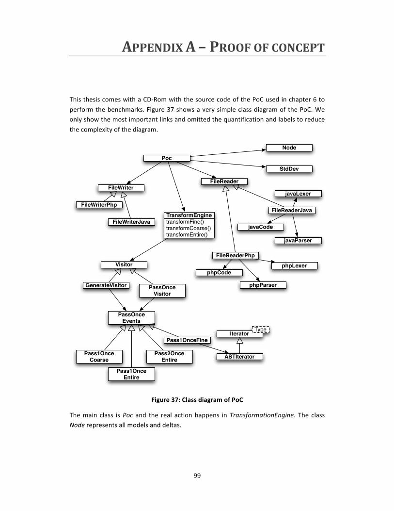
99
APPENDIX A – PROOF OF CONCEPT
This thesis comes with a CD‐Rom with the source code of the PoC used in chapter 6 to
perform the benchmarks. Figure 37 shows a very simple class diagram of the PoC. We only show the most important links and omitted the quantification and labels to reduce
the complexity of the diagram.
Figure 37: Class diagram of PoC
The main class is Poc and the real action happens in TransformationEngine. The class Node represents all models and deltas.
Poc
FileWriter
FileWriterJava
FileWriterPhp
StdDev
Pass1OnceEntire
Pass1OnceCoarse
Pass2OnceEntire
Pass1OnceFine
PassOnceEvents
ASTIterator
Iterator
javaCode
javaLexer
javaParser
phpCode
phpLexer
phpParser
Node
FileReader
FileReaderJava
FileReaderPhp
Visitor
PassOnceVisitor
GenerateVisitor
Type
transformFine()transformCoarse()transformEntire()
TransformEngine

100
Transformations are implemented with the visitor design pattern (Gamma, Helm, Johnson, & Vlissides, 1995). In fine‐grained model transformation the iterator design
pattern of (Gamma, Helm, Johnson, & Vlissides, 1995) is used to iterate over the different entities in the files.
In this appendix we also give some code fragments of the actual implementation to emphasize the most important elements. All code can also be found on the CD‐Rom.
POC.JAVA
1: class DeltaElement { public Node delta; public boolean timing; public boolean detail_timing; 5: public int type; public DeltaElement(Node d, boolean t, boolean dt, int tp) { delta = d; 10: timing = t; detail_timing = dt; type = tp; } } 15: Vector<DeltaElement> deltas = new Vector<DeltaElement>();
Listing 14: List with deltas
Listing 14 shows sample code how different deltas are collected. Those will be transformed as a batch. We first always start with an empty model so we have to
generate a model first before we can perform a change to benchmark. This way we are able to make different situations. The timing results are stored within the DeltaElement to be presented afterwards.
1: private static double transform(TransformEngine te, Node delta, int type) { Node model = ModelReader.open(te.getPath() + "revs/current.xml"); 5: double time = 0; switch (type) { case T_ENTIRE: time = te.transformEntire(model, delta); 10: break; default: case T_COARSE: time = te.transformCoarse(model, delta); break; 15: case T_FINE: time = te.transformFine(model, delta); break;

101
} 20: storeModel(te.getPath(), te.getTarget()); return time; }
Listing 15: Start of transformation
Listing 15 shows the start of a transformation. An XML file will be opened and read and after that a delta will be used to perform a transformation on both the source model
and the file system. The type of model transformation can be passed as a parameter to choose which approach should be used. After transformation the model will be stored to the file system again as a XML file. The transformation returns the execution time in
rounded nanoseconds.
TRANSFORMENGINE.JAVA
1: PassOnceVisitor po = new PassOnceVisitor(model); Pass1OnceEntire p1 = new Pass1OnceEntire(); po.setPassOnceHandler(p1); 5: // perform first pass long t = System.nanoTime(); delta.accept(po); long tmp = System.nanoTime() - t; time += tmp; 10: target = po.getTarget(); float x=tmp; 15: GenerateVisitor gv = new GenerateVisitor(model); Pass2OnceEntire p2 = new Pass2OnceEntire(fw); gv.setPassOnceHandler(p2); // perform second pass 20: t = System.nanoTime(); target.accept(gv); tmp = System.nanoTime() - t; time += tmp;
Listing 16: Entire model transformation
Listing 16 shows partial code of the function transformEntire(). Here we need two passes, the first pass performs the transformation on the model and the second pass generates files of the entire model. This is done with visitor‐classes which use interfaces
to push their events. The classes Pass1OnceEntire and Pass2OnceEntire implement the interface to perform the real actions of the transformation. The accept() calls on line 7 and line 21 start both transformations. The execution time of both calls is stored,
rounded and returned in the end (not visible).

102
1: PassOnceVisitor po = new PassOnceVisitor(model); Pass1OnceCoarse p1 = new Pass1OnceCoarse(fw); po.setPassOnceHandler(p1); 5: // perform first pass long t = System.nanoTime(); delta.accept(po); long tmp = System.nanoTime() - t; time += tmp; 10: target = po.getTarget(); float x=tmp; 15: // perform second pass t = System.nanoTime(); fw.writeFiles(); tmp = System.nanoTime() - t; time += tmp;
Listing 17: Coarse‐grained model transformation
Listing 17 shows partial code of the function transformCoarse(). It also contains two passes and uses also interfaces to push the events. The class Pass1OnceCoarse implements this interface to perform the real actions of the transformation. The
transformation starts at line 7 with the call to the accept() function. The call to writeFiles() on line 17 generates the files that are affected with the change. This is a linear list of files. Here also the execution time is stored, rounded and returned in the
end (not visible).
1: PassOnceVisitor po = new PassOnceVisitor(model); Pass1OnceFine pof = new Pass1OnceFine(fw, fr); po.setPassOnceHandler(pof); 5: // perform first pass long t = System.nanoTime(); delta.accept(po); float tmp = System.nanoTime() - t; 10: time += tmp; target = po.getTarget();
Listing 18: Fine‐grained model transformation
Listing 18 shows partial code of the function transformFine(). The class Pass1OnceFine implements the events of the visitor and the call to accept() on line 8 starts the
transformation. Since the fine‐grained model transformation only exists out of one pass this is the only step to be performed. For the implementation of the file handling we refer to the file Pass1OnceFine.java on the CD‐Rom.

103
FILEWRITERPHP.JAVA
1: protected void writeNode(FileOutputStream fos, Node node) { if (node.getTag().equals("page")) { writeLine(fos, "<?"); for (int i : node.getReferences().keySet()) { 5: for (Node n : node.getReferences().get(i)) { writeNode(fos, n); } } 10: write(fos, "?>"); } else if (node.getTag().equals("panel")) { writeLine(fos, "class " + node.getProperty("name") + " {"); for (int i : node.getReferences().keySet()) { 15: for (Node n : node.getReferences().get(i)) { writeNode(fos, n); } } 20: writeLine(fos, "}"); } else if (node.getTag().equals("field")) { writeLine(fos, "private $" + node.getProperty("name") + ";", 1); } 25: }
Listing 19: Writing files
Listing 19 shows a partial implementation of the class that performs the file generation
in coarse‐grained and entire model transformation. The list of files is iterated (not visible) and for each file this function is called. It is a recursive functions because nodes that are affected here can have references to other nodes. The function getTag()
determines the type of the node which is used to generate the correct code.
Top Related