


Languages
Pages
Legal

A Fractional Split Distribution Model for Statewide
Commodity Flow Analysis
Aruna Sivakumar and Chandra Bhat
Department of Civil Engineering, ECJ 6.8
University of Texas at Austin, Austin, Texas, 78712
Phone: (512) 471-4535, Fax: (512) 475-8744,
Email: [email protected], [email protected]
ABSTRACT
This paper proposes and applies a relatively simple, but comprehensive, approach to modeling
inter-regional commodity flow volumes. The approach estimates the fraction of commodity
consumed at each destination zone that originates from alternative production zones. The
resulting fractional split model for commodity flow distribution is more general in structure than
the typical gravity model used today for statewide freight planning. The empirical analysis in the
paper applies the fractional split model to analyze inter-regional commodity flows in Texas.

Sivakumar and Bhat
1
1. INTRODUCTION
The primary focus of statewide and metropolitan transportation planning processes over the past
several decades has been on passenger travel demand forecasting [see Cambridge Systematics,
Inc. (1)]. However, after the passage of the Intermodal Surface Transportation Efficiency Act
(ISTEA) of 1991, there has been increasing interest in freight modeling within statewide and
metropolitan planning efforts.
While freight modeling has been receiving increasing attention in state and metropolitan
planning efforts only relatively recently, research in the freight modeling area has a long history.
Many different quantitative approaches have been proposed for freight modeling in the literature,
of which three have received particular attention. These are: (1) trend analysis, (2) the inter-
agent interaction approach, and (3) the four-step approach1. Each of the three approaches listed
above is briefly discussed in turn in the next three sections [the reader is referred to Pendyala et
al. and Shankar and Pendyala for comprehensive and detailed reviews of freight modeling
approaches (4,5)].
1.1. Trend Analysis
The trend analysis approach examines current freight flow patterns, and the trend in freight flow
patterns over the past several years, to predict future flows [see, Middendorf et al. (6) and
Cambridge Systematics, Inc. (1)]. The trend analysis approach is conceptually straightforward,
is not data-intensive (because it uses readily available aggregate freight movement data), and is
easy to implement. However, it is inadequate in examining the effects on freight flows due to 1 In addition to these three approaches, the origin destination (OD) synthesis approach that estimates origin-destination flows from traffic and screen counts is also receiving increasing attention [see List and Turnquist (2); Nozick, Turnquist, and List (3)]. However, this synthesis approach is not directly relevant to the current paper because it does not attempt to explain the fundamental impact of economic, demographic, and cost related forces on freight flows.

Sivakumar and Bhat 2
large-scale shifts in economic forces affecting freight movement patterns and due to
improvements in the existing transportation infrastructure along freight corridors.
1.2. The Inter-Agent Interaction Approach
The fundamental basis of the inter-agent interaction approach is that freight travel demand is a
result of commodity movements from commodity producers to commodity consumers. Two
types of inter-agent interaction formulations may be identified: spatial price equilibrium models
and network equilibrium models. Spatial price equilibrium models represent the spatial
distribution of producers and consumers by location-specific supply and demand functions, and
assume that shippers determine the commodity flow between regions based on the cost at the
origin end, the transportation cost between the origin and the destination region, and the
commodity cost at the destination end [see Friesz et al. (7); Harker (8)]. The interaction between
shippers and carriers is not considered in spatial price equilibrium models. Network equilibrium
models, on the other hand, focus on shipper-carrier interactions. They obtain freight flows by
origin-destination pairs and by carrier based on the concept of cost-minimizing behavior on the
part of shippers (9,10,11,12). Once the carrier-specific freight flows by origin-destination pair
are determined, each carrier decides on the routing of freight flows based on a traditional trip
assignment model.
The inter-agent interaction models are quite comprehensive in their treatment of the
multi-agent interaction process characterizing the mechanism by which economic and marketing
forces shape and influence freight flows. These models can use individual-level shipper and
carrier data [see (11,12)] or can use aggregate representations of shippers and carriers [see
Guelat et al. (13); Marchant (14)]. But the inter-agent interaction models are data-intensive and

Sivakumar and Bhat 3
complex to implement. While these models have tremendous promise in the longer term, they
are less likely to be adopted by state and metropolitan planning organizations in the short term.
1.3. The Four-Step Approach
The four-step approach to freight modeling is an adaptation of the traditional urban passenger
travel demand modeling system (1,15,16). The primary steps in the process are freight
generation, distribution, mode choice, and route assignment. While the factors and decision-
making agents driving freight flow and passenger travel are quite different, the comparison with
the four-step urban passenger model provides a reasonable framework for freight modeling
(17,18).
The four-step freight modeling approach may use disaggregate individual shipment data
or aggregate freight movement data in the analysis [see Zlatoper and Austrian (19), and Winston
(20), for detailed reviews of freight models using disaggregate and aggregate data]. Several
research efforts in the past decades have employed disaggregate freight data [see Winston
(20,21)]. However, most of these efforts have been confined to the modal split step within the
four-step process. Also, modeling with disaggregate data is seldom undertaken in practice
because disaggregate data on individual shipments are often proprietary in nature, and difficult to
acquire. On the other hand, aggregate data are much easier to acquire. Consequently, the most
common practice in statewide and metropolitan freight planning efforts is to use aggregate data
within the four-step approach.
Sivakumar and Bhat 4
1.4. Objective of Paper
The objective of this paper is to propose and demonstrate the application of a relatively simple,
but comprehensive, approach to statewide freight flow modeling in the spirit of an aggregate
level four-step planning process. The specific focus in the current paper is on modeling freight
flows between production-consumption nodes, not on modal split or vehicle trip assignment. In
particular, a fractional split model is formulated to determine the fraction of commodity
consumed in a county that is produced at each county in the planning region. The fractional split
model is empirically estimated for the state of Texas using inter-county commodity flow data,
and supplementary socio-economic and transportation system data.
The rest of this paper is structured as follows. The next section provides an overview of
earlier four-step freight models in a statewide planning context and positions the current research
within this broader context. Section 3 presents the fractional split model structure and discusses
the technique used in model estimation. Section 4 introduces the data sources used in the
empirical analysis, describes the data assembly procedures, and presents the empirical results.
Section 5 summarizes the important findings from the study.
2. FOUR-STEP FREIGHT MODELS AND THE CURRENT RESEARCH
2.1. Structure of Four-Step Models
The four-step freight models that have been developed and used in statewide freight planning
efforts may be broadly classified into three categories: vehicle-based models, commodity-based
models, and combined vehicle and commodity-based models (18).
The vehicle-based models focus on truck traffic, and follow the traditional steps of trip
generation, trip distribution, and highway assignment. The vehicle-based modeling approach has

Sivakumar and Bhat 5
been applied for statewide planning in New Jersey and Phoenix (18,22). A problem with
vehicle-based models is that they are not policy-sensitive, since they are unable to reflect
changes in growth rates by commodity class. Fundamentally, they fail to recognize that freight
travel is related to commodity movement, not truck movement. However, they are useful in
estimating short-distance service vehicle trips (such as package delivery and pick-up trips).
The commodity-based models emphasize and predict the movement of commodity by
class, and subsequently translate commodity movements to vehicle traffic by mode. The trip
generation stage involves the estimation of linear regression models, spatial input-output models
[see (23,24)], or commodity rates to predict commodity production and consumption levels at
each analysis zone by commodity class. The usual gravity model formulation, with highway
distance as the measure of travel impedance, is used in trip distribution. This is followed by the
conversion from commodity flows to vehicle flows using commodity-specific tonnage-to-vehicle
factors. Traffic assignment is undertaken using an all-or-nothing assignment technique.
Examples of the application of commodity-based models include the statewide freight models in
Indiana, Kansas, Michigan, Wisconsin, and Portland. As should be evident, the commodity-
based modeling approach is a commonly used approach in statewide freight planning efforts.
The approach recognizes the sensitivity of commodity flow to economic and transportation
system forces, and emphasizes commodity flow as the underlying determinant of freight traffic.
However, commodity-based models do not estimate short-distance service vehicle trips, which
may dominate intra-regional and urban freight vehicle movements. In addition, the use of
commodity-based models requires an approach to estimate empty trips. Some practitioners have
considered empty trips as a separate commodity; however, this is inconsistent with the
fundamental basis of commodity flow models that vehicle trips (both loaded and empty) are a
Sivakumar and Bhat 6
result of the logistics of commodity movements. Hautzinger (25) and Kim and Hinkle (26)
suggest probabilistic models that calculate the probability of truck backhauling as a function of
commodity volumes, distance, truck capacity, and backhauling cost. But, the issue of addressing
empty trips within the commodity-based approach remains an important area for further
research.
The combined vehicle and commodity-based models integrate the strength of the vehicle-
based method in estimating short-distance service vehicle trips with the strength of the
commodity-based method in estimating long-distance commodity flow-driven vehicle trips.
2.2. The Current Research
The current research focuses on a statewide freight planning model for the state of Texas, and
takes the structure of a commodity-based model. The model formulation and empirical analysis
are specifically targeted toward the trip generation and trip distribution steps.
In earlier applications of the commodity-based model for statewide freight planning,
commodity generation has included the estimation of production and consumption levels at each
geographic analysis zone by commodity type. The commodity distribution step allocates the
production at each zone among various consumption zones using a gravity model. In contrast,
the current study formulates a fractional split model for distribution within a modeling
framework that first determines consumption levels at each zone in a commodity generation step,
[using linear regression or spatial input-output models, see (22)], and then uses the fractional
split distribution model to estimate the fraction of consumption at the destination zone that
originates at each of the production zones. The motivation behind this approach is two-fold.
First, freight movement is fundamentally generated by the demand for consumption of

Sivakumar and Bhat 7
commodities at the destination (or attraction) end, which is met by the flow of commodities from
one or more origin (or production) points [see Ogden (27)]. Second, the fractional split
distribution formulation recognizes the impact of the location pattern of zones on the amount of
commodities produced at each zone [see Sivakumar (28) for a detailed discussion].
In addition to the advantages of the fractional split formulation discussed above, our
proposed approach is also able to (a) accommodate multiple zonal size measures to reflect the
production potential in a zone, (b) incorporate the travel characteristics of multiple freight modes
in determining commodity flow interchanges, and (c) recognize interactions of production zone
attributes and travel impedance.
3. FRACTIONAL SPLIT FREIGHT DISTRIBUTION MODEL
3.1. Background and Estimation Approach
The dependent variable in the current analysis represents the fraction of freight consumed at a
zone that is produced at each origin zone. The sum of the fractions across all production zones
(for each consumption zone) is equal to one, and each fraction is bounded between zero and one.
Further, one or more of the fractions may take the boundary values of zero or one; that is, some
production zones may not serve a consumption zone, or the consumption at a destination zone
may be entirely served by a single production node.
Mathematically, let qiy be the fraction of freight consumed at destination zone q (q =
1,2,...,J) that is produced from origin zone i (i = 1,2,...,J). By definition, for each destination
zone, the following must be true:
∑ =≤≤i
qiqi yy .1 ,10 (1)

Sivakumar and Bhat 8
Let the fraction qiy be a function of a vector qix of relevant explanatory variables associated
with attributes of the origin zone i, the travel impedance between zones q and i, and interactions
of zonal attributes with the travel impedance. A common approach to analyzing fractional
dependent variables is to model the log-odds ratio as a linear function of the explanatory
variables [for example, see Bhat and Misra (29)]. However, this approach does not address the
situation where an origin zone does not contribute to the consumption at a destination mode [see
Sivakumar (28)].
The model we propose here for freight distribution modeling is a polychotomous
extension of the binary fractional split model proposed by Papke and Wooldridge (30). Consider
the following econometric specification:
∑=
=<<β=J
iiiqJqqiqJqqqi GGxxxGxxxyE
12121 . 1 (.) ,1(.)0 ),,...,,,( ),...,,|( (2)
(.)iG (i=1,2,…,J) in the above equation is a pre-determined function. The properties specified
above for (.)iG ensure that the predicted fractional freight flows will lie in the interval (0,1) and
will sum to 1 across origin zones for each destination zone. The econometric model in equation
(2) is well-defined, even if qiy takes the value of 0 or 1 with positive probability.
The β parameter vector in the conditional mean model of equation (2) is estimated using
a quasi-likelihood estimation approach [see Gourieroux et al. (31)]. Specifically, we use the
multinomial log-likelihood function in the quasi-estimation:
‹q(β) = ).,...,,,( log 211
qJqqi
J
iqi xxxGy β∑
= (3)
The multinomial quasi-likelihood estimator used above belongs more generally to the linear
exponential family (LEF). Gourieroux et al. prove the strong consistency and asymptotic

Sivakumar and Bhat 9
normality of the parameter estimator of β obtained by maximizing qΣ‹q(β), as long as (and if
and only if) ‹q(β) belongs to the LEF [see also Wooldridge (32)].
3.2. Model Structure
We use a multinomial logit functional form for Gi in the fractional split model of equation (2)
since this structure is easy to program and implement2. We then write equation (2) as:
[ ]
[ ], ),...,,,()|(
1
)( )log(
)( )log(
1
21
∑∑=
δ′+α+γ
δ′+α+γ
=
β′
β′
==β= J
j
zHfD
zHfD
J
j
x
x
Jqiqiqiqjqjj
qiqii
qj
qi
e
e
e
exxxGxyE (4)
where iD is a composite size measure for origin zone i and qiH is a composite impedance
measure for travel between nodes q and i. qiz is a vector that may include (a) non-size attributes
specific to zone i, (b) interactions of non-size zonal attributes with the composite impedance
variable, (c) the interaction of the composite zonal size variable with the composite impedance
variable, and (d) interactions of the attributes of zones q and i. γ and α are scalars, and δ is a
vector, to be estimated. In the following two sections, we discuss the functional forms for the
composite size and composite impedance components of Equation (4).
3.2.1. Composite Size Term
The size measure iD in Equation (4) represents the number of elemental commodity production
points within zone i. However, the number of elemental production points within zone i is not
easily quantifiable. But we can “proxy” iD by a set of observable size variables such as
2 The multivariate normal distribution may also be used, but is more cumbersome relative to the multinomial logit. Furthermore, the assumption of independence within a multivariate normal distribution leads to an almost identical model as the multinomial logit.

Sivakumar and Bhat 10
employment by sector in zone i, zonal land area, and zonal population. If id is a vector of
individual size measures, we can develop the composite size measure as , ii dD η′= where η is
a vector of parameters to be estimated in the fractional split model [for identification reasons,
one element of η has to be normalized to one; see Bhat et al. (33)].
The elements of the vector η have to be non-negative, and this restriction is
operationalized in our estimation by reparameterizing η as )exp(µ . The reparameterization is
helpful because the elements of µ are unbounded. Once the vector µ is estimated, the
exponential transformation of the elements of this vector provides the estimates of the elements
of the vector η . The standard errors of each element of the η vector may be obtained using a
linear Taylor series approximation applied to the standard errors of the elements of µ .
3.2.2. Composite Impedance Term
The function f(.) used in the composite impedance measure in Equation (4) is generally specified
to be either linear ])([ qiqi HHf = or log-linear )]ln()([ qiqi HHf = [see Fotheringham (34)]. The
linear form implies that the marginal deterrence due to travel impedance is independent of the
existing impedance level, while the log-linear form implies that the marginal deterrence
decreases as the existing travel impedance increases.
The composite measure itself (i.e., qiH ) may comprise multiple individual impedance
measures such as travel time and distance. In the current analysis, we use distance as the only
measure of impedance. Travel time is not used as a measure of impedance because the delivery
of a particular consignment of commodities can take several days due to coordination with the
Sivakumar and Bhat 11
delivery of other consignments, even though the distance of the commodity movement may be
very small [see Ogden for a discussion of this point (27)].
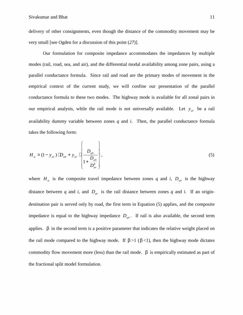
Our formulation for composite impedance accommodates the impedances by multiple
modes (rail, road, sea, and air), and the differential modal availability among zone pairs, using a
parallel conductance formula. Since rail and road are the primary modes of movement in the
empirical context of the current study, we will confine our presentation of the parallel
conductance formula to these two modes. The highway mode is available for all zonal pairs in
our empirical analysis, while the rail mode is not universally available. Let qiry be a rail
availability dummy variable between zones q and i. Then, the parallel conductance formula
takes the following form:
, 1
)1(
+⋅+⋅−=
βqir
qih
qihqirqihqirqi
DD
DyDyH (5)
where qiH is the composite travel impedance between zones q and i, qihD is the highway
distance between q and i, and qirD is the rail distance between zones q and i. If an origin-
destination pair is served only by road, the first term in Equation (5) applies, and the composite
impedance is equal to the highway impedance qihD . If rail is also available, the second term
applies. β in the second term is a positive parameter that indicates the relative weight placed on
the rail mode compared to the highway mode. If β >1 (β <1), then the highway mode dictates
commodity flow movement more (less) than the rail mode. β is empirically estimated as part of
the fractional split model formulation.

Sivakumar and Bhat 12
To summarize, the parameters to be estimated in the fractional split distribution model of
Equation (4) include the scalars γ and α , the vector δ , the vector η embedded in the composite
size variable, and the scalar β embedded in the composite impedance variable. The estimation
is achieved by maximizing the quasi-likelihood function in Equation (3) using the GAUSS
matrix programming language.
4. DATA SOURCES AND ASSEMBLY
4.1. Data Sources
Several data sources were used in the fractional split distribution model estimation. These
include: a) the Reebie TRANSEARCH Freight Database, b) County Business Patterns compiled
by the U.S. Census Bureau, c) the U.S. Census Bureau Population projections, d) the Regional
Economic Information System (REIS) database compiled by the U.S. Bureau of Economic
Analysis, and e) TransCAD geographic maps and datasets. In the next two sections, we discuss
the Reebie data and the other data sources.
4.1.1. The Reebie TRANSEARCH Freight Database
The primary data resource in this study is the 1996 Reebie data, a proprietary database of county-
to-county commodity movements throughout the United States. It is compiled and produced
annually, based on surveys of major shippers and carriers in the freight industry, the Census of
Transportation Commodity Flow Survey, the Annual Rail Carload Waybill Sample, and several
other traffic data flow sources. The data used in the current study is a subset of the nationwide
Reebie data that focuses on Texas-related commodity movements.

Sivakumar and Bhat 13
The database comprises four files, each providing inter-zonal freight movements by the
four major transportation modes (road, rail, water, and air). These four files, when taken
together, provide information regarding annual commodity flows from (a) Texas counties to
other parts of the country represented by external unit codes (i.e., Texas county to EUC flows),
(b) Other parts of the country to Texas counties (i.e., EUC to Texas county flows), and (c) Texas
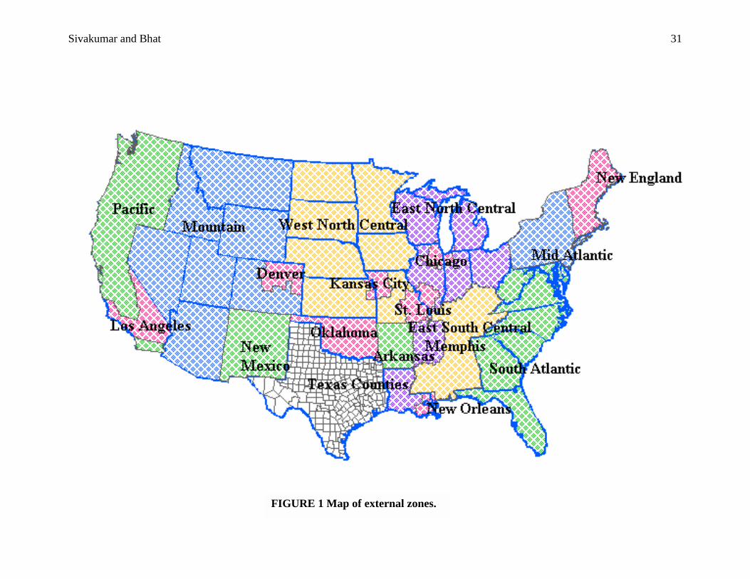
county to Texas county. The Reebie data identifies 254 Texas counties. The EUCs, as
represented in the Reebie Texas database, include 19 aggregate zones. A map of these external
zones is presented in Figure 1. A limitation of the Reebie data available to us is that it does not
provide information on interchanges between Texas counties and Mexico; rather it only provides
aggregate information regarding flows from/to Texas as a whole. Therefore, we are unable to
consider Mexico as an external station in the current analysis.
The Reebie data identifies movements by 50 commodity types based on the STCC2 (two
digit Standard Transportation Commodity Classification) classification code, which were
organized into 7 commodity groups for the current analysis: (1) Agricultural and Related
Products, (2) Hazardous Materials, (3) Construction Materials, (4) Food and Related Products,
(5) Manufacturing Products, (6) Machinery and Equipment, and (7) Mixed Freight Shipments.
To summarize, the Reebie data provides information regarding commodity flows
between Texas counties and between Texas counties and external stations. For the current
analysis, the fraction of commodity consumption at a zone that is produced at each of the other
zones is computed and is used as the dependent variable.
Sivakumar and Bhat 14
4.1.2. Other Sources of Data
This section discusses the data sources other than the Reebie data used in the analysis. These
supplementary data sources include the county business pattern database, the U.S. Census
Bureau population projections, the REIS database, and TransCAD-related data.
The County Business Pattern database is maintained by the U.S. Census Bureau and has
been published every year since 1946 at the county, state, and national levels. The data provides
county-specific information on economic indicators, including establishment counts by
institution size and mid-March employment figures. This dataset represents one of our sources
of socio-economic information on Texas counties.
The U.S. Census Bureau population projections provide county-level population
predictions based on decennial census counts. The population figures used in our analysis
correspond to 1996, since this was the year the Reebie data was compiled.
The REIS (Regional Economic Information System) database, assembled by the Bureau
of Economic Analysis, provides local area economic data for states, counties, and metropolitan
areas for the period 1969-1998. The current study uses county-level statistics of employment by
sector, including farm and non-farm employment, mining, manufacturing, construction, services
employment, etc.
The TransCAD geographic maps and datasets are used to determine the centroidal
distances between zones. U.S. highway and rail line layers embedded within TransCAD are
used to compute the interzonal distances along the road and rail networks. The rail mode is
considered to be unavailable to a zone if there is no rail line running through the zone or within
50 miles of the zone. It is also assumed that the rail mode services zones through which there is

Sivakumar and Bhat 15
a rail line3. Intrazonal freight interchanges are assigned a distance equal to half the distance from
that zone to its closest neighboring zone. The geographic areas of the counties are also
computed from TransCAD-embedded maps.
4.2. Variable Specification
Three of the seven commodity groups in Table 2 are chosen for analysis in this paper based on
having large volumes of total freight tonnage and a relatively high representation of inter-
regional flows. The three chosen commodity groups are a) Agricultural and Related Products
(ARP), b) Construction Materials (CM), and c) Food and Related Products (FRP). Separate
fractional split models are developed for each of the commodity groups.
The dependent variable in the analysis for each commodity group is the fraction of total
tonnage consumed in a zone (a Texas county or an EUC) that is produced from each of the 254
Texas counties and the 19 EUCs. However, the Reebie data available to us did not have the
EUC-EUC commodity flow interchanges. Thus, the number of production (origin) zone
alternatives is 273 (254 Texas counties plus 19 EUCs) for each Texas county consumption
(destination) zone and 254 for each EUC consumption zone.
The number of consumption zones (i.e., the number of observations in estimation) varies
across the commodity groups because some zones do not “consume” certain commodity types.
The number of consumption zones is 124 for the ARP commodity group, 268 for the CM
commodity group, and 261 for the FRP commodity group.
The independent variables considered in the analysis include production zone size
variables (employment by sector, area, population, number of establishments, and annual
payroll), impedance variables (rail and road distances), and non-size production zone variables 3 An improved representation of the rail network would be a useful area for future work.

Sivakumar and Bhat 16
(including employment rate, population density, establishment density, presence of a port in
zone, and per capita payroll).
The impedance variables (rail and road distances) have been obtained for all zone-to-zone
pairs (including Texas county to EUC pairs). However, the zonal size and non-size measures are
defined only for Texas counties and not for EUCs. The EUCs are spatial representations that do
not clearly correspond to aggregations of smaller spatial units for which economic data are
available. In our analysis, we introduce 19 alternative-specific EUC constants to accommodate
the different size and non-size characteristics of the 19 EUCs.
The final set of variables and their method of inclusion in the fractional distribution
model was determined based on a systematic process of eliminating variables found to be
statistically insignificant in previous specifications and based on considerations of data fit.
4.3. Empirical Results and Interpretation
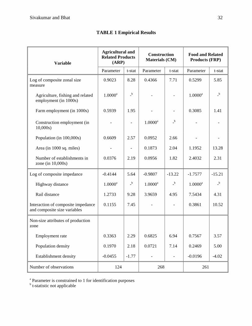
The final model specifications are presented in Table 1. These results are discussed by variable
group below. In the following discussion, we do not present the 19 EUC-specific constants
because these constants do not have any substantive interpretation. These constants may be
obtained directly from the authors.
4.3.1. Composite Size Measure
The coefficients on the (log) composite size measure are positive and statistically significant for
all three commodity groups, as expected. Among the groups, size of the production zone is more
important in determining commodity movement for the ARP group relative to the other two
groups. In fact, the coefficients on the size variable indicate that the fraction of consumption at a
Sivakumar and Bhat 17
zone produced from other zones is almost proportional to the size of the production zone for the
ARP group, but is about proportional to the square root of the size of the production zone for the
other two groups.
In addition to the difference in size effects across the three groups, there are also
differences in the zonal attributes characterizing zonal size. As can be observed from Table 1,
the variables characterizing size for the ARP group include agricultural-related employment,
farm employment, zonal population, and number of establishments in the zone. The coefficient
on farm employment indicates that 1 unit of farm employment is equivalent to about 0.6 units of
agricultural-related employment in terms of zonal size representation. This is intuitive, since
agricultural-related employment should contribute more to the “production-power” of a zone for
agricultural-related products than farm employment. The relative effects of other variable vis-à-
vis the agricultural-related employment variable is not as direct because of the difference in units
and nature of the other variables. After normalizing for differences in units, the results suggest
that about 150 new members in the population have the same impact as one additional
agricultural employee, while it takes 265 new establishments to have the same impact as one
additional agricultural employee. Clearly agricultural employment dominates as the main
determinant of the size of a zone for production of agricultural-related products.
The interpretation of the contribution of the individual size variables to the overall zonal
size measure for the construction materials (CM) and food-related product (FRP) groups may be
derived in the same manner as for the ARP group. For the construction group, the parameters
clearly indicate the dominance of construction employment in determining the production
“power” of a zone. For the food group, the results show that 1 unit of farm employment is
equivalent to about 0.3 units of agriculture employment, 1 unit of area is equivalent to about 1.2
Sivakumar and Bhat 18
units of agricultural employment, and 1 establishment is equivalent to about 0.25 units of
agricultural employment. A comparison between the ARP and FRP groups suggests that farm
employment is more of a size factor for production of agricultural commodities than for food-
related commodities.
4.3.2. Composite Impedance and Impedance-Size Interaction
Two functional forms for the composite impedance variable were tested: the linear and the log-
linear form. The log-linear form was far superior to the linear form and is the one retained in the
final specification in Table 1. As expected, the coefficient value on the (log) composite
impedance variable is negative and highly significant for all commodity groups. That is, the
fractional freight flow from a distant production zone to a consumption zone is smaller than from
a closely located production zone, everything else being equal.
The importance of the rail mode in characterizing the composite impedance for
commodity movement is provided by the magnitude of the parameter on rail distance (see
Section 3.2.2 for a discussion). The parameter is greater than 1 for all groups, indicating that the
rail mode determines commodity flow movement less than the highway mode. However, there
are differences in the contribution of the rail mode across the groups. Specifically, the rail
distance dictates commodity movement substantially more for the ARP group than the other
groups. This suggests that rail improvements are best positioned in spatial corridors with heavy
movement of agriculture-related products. On the other hand, the rail mode is literally a non-
factor for the food and related products category.
The effect of impedance on commodity flows depends on the impedance coefficient as
well as the interaction effect of the composite impedance variable with the size measure. The
Sivakumar and Bhat 19
latter interaction effect is statistically significant only for the ARP and FRP groups. For both
these groups, the sign on the interaction effect indicate that the impedance deterrence effect is
smaller if the production region is of large size, possibly reflecting economies of cost in shipping
large amounts of commodities from a large production center.
The net effect of travel impedance for any production zone can be computed from the
coefficients on the composite impedance term and the impedance-size interaction effect. For
both the ARP and FRP groups, this net effect stays negative for all zonal pairs in the sample;
thus, high impedance always has a deterring effect on commodity flows. Between the two
commodity groups, the net impedance deterrence is always higher for the FRP group. This may
be a reflection of the perishable nature of food products, because of which food products may be
moved shorter distances than agricultural products.
A comparison of the impedance-related coefficients between the ARP and CM groups
shows that the impedance deterrence effect is lower for the former group relative to the latter.
This may be a reflection of the higher transportation cost per unit of distance for the heavier CM
group compared to the lighter ARP group. Between the CM and FRP groups, the relative effect
of impedance depends upon the size of the zone. The deterrence due to distance is larger for the
FRP group for commodities originating from small to medium food production zones. But the
deterrence effect is smaller for the FRP group for commodities originating in large food
production zones.
4.3.3. Non-Size Attributes of Production Zone
Among the non-size attributes, the effect of employment rate indicates a higher commodity flow
from zones with high employment rates. This relationship holds for all commodity groups, and
Sivakumar and Bhat 20
presumably is a general reflection of high productivity levels associated with high employment
rates. The results also indicate a positive effect of population density on commodity flows
originating from a zone. Establishment density, on the other hand, has a negative impact on
commodity flows originating from a zone (for the ARP and food groups). This result is a little
surprising, but may be a manifestation of the aggregate nature of data on establishments. Ideally,
it would be useful to have information on establishments by sector (as for employment), but we
were unable to obtain such data within the scope of the current study.
4.4 Evaluation of Fit
In this section, we evaluate the fit of the fractional split distribution model with the typical
gravity model used in practice today for statewide freight planning. The typical gravity model
would include only the logarithm of road distance, the 19 EUC-specific constants, and a single
size measure [with the coefficient on the size measure constrained to one; see Bhat et al. (33)].
Thus the specifications in Table 1 are more general than the gravity models used in practice
today.
A measure of fit of a model in the estimation sample is the adjusted likelihood ratio index
or McFadden’s adjusted 2R defined as follows [see Windmeijer (35)]:
,)0(
)ˆ(12
LQL −β−=ρ (6)
where )ˆ(βL and L(0) are the log-likelihood function values at convergence and at equal shares,
respectively, and Q is the number of parameters estimated in the model. From a formal
statistical fit standpoint, the choice specifications in Table 1 are compared to the typical gravity
model used today in statewide freight planning using a nested likelihood ratio test.
Sivakumar and Bhat 21
The measures of fit are provided in Table 2. The fractional split specification has a
higher adjusted likelihood ratio index compared to the gravity model for all commodity groups
(agricultural employment is used as the single size measure for the ARP and FRP groups in the
gravity model, and construction employment is used as the single size measure for the CM
group). The nested likelihood ratio index statistic for testing the fractional split model with the
gravity model is provided in the last row of Table 2. A comparison of these statistics with the
chi-squared table values corresponding to the additional number of parameters estimated in the
fractional split structures very clearly indicates the better data fit of the proposed model.
5. CONCLUSIONS
This paper proposes and applies a relatively simple, but comprehensive, approach to modeling
inter-regional commodity flow volumes. The approach estimates the fraction of commodity
consumed at each destination zone that originates from production zones. The resulting
fractional split model for commodity flow distribution is more general in structure than the
typical gravity model used today for statewide freight planning.
The empirical part of the paper demonstrates an application of the proposed fractional
split model to analyze commodity flows between 254 Texas counties and between the Texas
counties and 19 external stations representing different parts of the U.S. The empirical results
provide important insights into the determinants of inter-regional commodity flow in Texas.
Specifically, the results can be used to predict future commodity flow patterns due to changes in
the socio-economic characteristics of zones and the transportation infrastructure. Further, the
results can also aid in transportation policy analysis to identify key transportation infrastructure
changes to alleviate truck-related traffic congestion on roadways.

Sivakumar and Bhat 22
In an evaluation of data fit, the results indicate that the proposed fractional split structure
outperforms the typical gravity structure used today in statewide freight planning. More
generally, the results demonstrate the value of the fractional split structure for commodity flow
modeling. The structure is intuitive, relatively simple to estimate, and is capable of
accommodating a large number of factors influencing commodity flow demand.
ACKNOWLEDGEMENTS
The authors are grateful to Lisa Weyant for her help in typesetting and formatting this document.
Four reviewers provided valuable comments on an earlier version of this paper.

Sivakumar and Bhat 23
REFERENCES
1. Cambridge Systematics, Inc. A Guidebook for Forecasting Freight Transportation Demand.
NCHRP Report 388, Transportation Research Board, National Academy Press, 1997.
2. List, G.F., and M.A. Turnquist. A GIS-Based Approach for Estimating Truck Flow Patterns
in Urban Settings. Journal of Advanced Transportation, Vol. 29, No.3, 1994, pp. 281-298.
3. Nozick, L.K., Turnquist, M.A., and G.F. List. Trade Pattern Estimation Between the United
States and Mexico. Transportation Research Circular, Issue 459, 1996, pp. 74-86.
4. Pendyala, R.M., Shankar, V.N., and R.G. McCullough. Freight Travel Demand Modeling:
Synthesis of Approaches and Development of a Framework. Transportation Research
Record 1725, TRB, National Research Council, Washington, D.C., 2000, pp. 9-16.
5. Shankar, V.N. and R.M. Pendyala. Freight Travel Demand Modelling: Econometric Issues
in Multi-level Approaches. In D. Hensher and J. King (eds) The Leading Edge of Travel
Behaviour Research, Chapter 38, Elsevier Science, The Netherlands, pp. 629-644 (in
press).
6. Middendorf, D.P., Jelavich, M., and R.H. Ellis. Development and Application of Statewide,
Multimodal Freight Forecasting Procedures for Florida. Transportation Research Record
889, TRB, National Research Council, Washington, D.C., 1982, pp. 7-14.
7. Friesz, T.L., Tobin, R.L., and P.T. Harker. Predictive Intercity Freight Network Models:
The State of the Art. Transportation Research, Vol. 17A, No. 6, 1983, pp. 409-417.
8. Harker, P.T. The State of the Art in the Predictive Analysis of Freight Transport Systems.
Transport Reviews, Vol. 5, No. 2, 1985, pp. 143-164.
9. Bronzini, M.S. Evolution of a Multimodal Freight Transportation Network Model.
Proceedings. Transportation Research Forum, Vol. 21, Oxford Ind., 1980, pp. 475-485.
Sivakumar and Bhat 24
10. Friesz, T.L., Viton, P.A., and R.L. Tobin. Economic and Computational Aspects of Freight
Network Equilibrium Models: A Synthesis. Journal of Regional Science, Vol. 25, No. 2,
1985, pp. 29-49.
11. Harker, P.T. and T.L. Friesz. Prediction of Intercity Freight Flows, I: Theory.
Transportation Research, Vol. 20B, No. 2, 1986, pp. 139-153.
12. Harker, P.T. and T.L. Friesz. Prediction of Intercity Freight Flows, II: Mathematical
Formulation. Transportation Research, Vol. 20B, No. 2, 1986, pp. 155-174.
13. Guelat, J., Florian, M., and T.G. Crainic. A Multimode Multiproduct Network Assignment
Model for Strategic Planning of Freight Flows. Transportation Science, Vol. 24, No. 1,
1990, pp. 25-39.
14. Marchant, M.A. Analysis of the Effects of Rising Transportation Costs on California’s
Fresh Fruit and Vegetable Markets. Journal of the Transportation Research Forum, Vol.
32, No. 1, 1991, pp. 17-32.
15. Memmott, F.W. Application of Statewide Freight Demand Forecasting Techniques.
NCHRP Report 260, Roger Creighton Associates, Transportation Research Board,
National Academy Press, 1983.
16. Holguín-Veras, J. and E. Thorson. Trip Length Distributions in Commodity-Based and
Trip-Based Freight Demand Modeling. Transportation Research Record 1707, TRB,
National Research Council, Washington, D.C., 2000, pp. 37-48.
17. Kurth, D., Donnelly, R., Arens, B., Hamburg, J., and W. Davidson. A Research Process for
Developing a Statewide Multimodal Transportation Forecasting Model. Final Report
prepared by Barton-Aschman Associates, for the New Mexico State Highway and
Transportation department, Santa Fe, August 1991.

Sivakumar and Bhat 25
18. Cambridge Systematics, Inc. Florida Intermodal Statewide Highway Freight Model.
Technical Memorandum Task I – Review of Current Freight Models, 2000.
19. Zlatoper, T.J., and Z. Austrian. Freight Transportation Demand: A Survey of Recent
Econometric Studies. Transportation, Vol. 16, 1989, pp. 27-46.
20. Winston, C. The Demand for Freight Transportation: Models and Applications.
Transportation Research, Vol. 17A, No. 6, 1983, pp. 419-427.
21. Winston, C. A Disaggregate Model of the Demand for Intercity Freight Transportation.
Econometrica, Vol. 49, 1981, pp. 981-1006.
22. Ruiter, E.R. Development of an Urban Truck Travel Model for the Phoenix Metropolitan
Area. Final Report, Cambridge Systematics, 1992.
23. Sorratini, J.A. Estimating Statewide Truck Trips Using Commodity Flows and Input-
Output Coefficients. Journal of Transportation and Statistics, 2000, pp. 53-67.
24. Sorratini, J.A. and R.L. Smith Jr. Development of a Statewide Truck Trip Forecasting
Model Based on Commodity Flows and Input-Output Coefficients. Transportation
Research Record 1707, TRB, National Research Council, Washington, D.C., 2000, pp. 49-
55.
25. Hautzinger, H. The Prediction of Interregional Goods Vehicle Flows: Some New
Modelling Concepts. Ninth International Symposium on Transportation and Traffic
Theory, VNU Science Press, 1984, pp. 375-396.
26. Kim, T.J., and J.J. Hinkle. Model for Statewide Freight Transportation Planning.
Transportation Research Record 889, TRB, National Research Council, Washington, D.C.,
1982, pp. 15-19.
Sivakumar and Bhat 26
27. Ogden, K.W. The Distribution of Truck Trips and Commodity Flow in Urban Areas: A
Gravity Model Analysis. Transportation Research, Vol. 12, 1978, pp. 131-137.
28. Sivakumar, A. A Fractional Split Distribution Model for Statewide Commodity Flow
Analysis. Thesis, The University of Texas at Austin, 2001.
29. Bhat, C.R., and R. Misra. Discretionary Activity Time Allocation of Individuals Between
In-home and Out-of-home and Between Weekdays and Weekends. Transportation, Vol.
26, No. 2, 1999, pp. 193-209.
30. Papke, L.E., and J.M. Wooldridge. Econometric Methods for Fractional Response
Variables with an Application to 401(k) Plan Participation Rates. Journal of Applied
Econometrics, Vol. 11, 1996, pp. 619-632.
31. Gourieroux, C., Monfort, A., and A. Trognon. Pseudo Maximum Likelihood Methods:
Theory. Econometrica, Vol. 52, 1984, pp. 681-700.
32. Wooldridge, J.M. Specification Testing and Quasi-Maximum Likelihood Estimation.
Journal of Econometrics, Vol. 48, 1991, pp. 29-55.
33. Bhat, C.R., Govindarajan, A., and V. Pulugurta, V. (1998). Disaggregate Attraction-End
Choice Modeling: Formulation and Empirical Analysis. Transportation Research Record
1645, TRB, National Research Council, Washington, D.C., 1998, pp. 60-68.
34. Fotheringham, A.S. Modeling Hierarchical Destination Choice. Environment and Planning,
Vol. 18A, 1986, pp. 401-418.
35. Windmeijer, F.A.G. Goodness-of-Fit Measures in Binary Choice Models. Econometric
Reviews, Vol. 14, 1995, pp. 101-116.

Sivakumar and Bhat 27
LIST OF FIGURES
FIGURE 1 Map of external zones. LIST OF TABLES TABLE 1 Empirical Results
TABLE 2 Measures of Fit
Sivakumar and Bhat 31
FIGURE 1 Map of external zones.
Sivakumar and Bhat 32
TABLE 1 Empirical Results
Agricultural and Related Products
(ARP)
Construction Materials (CM)
Food and Related Products (FRP)
Variable Parameter t-stat Parameter t-stat Parameter t-stat
Log of composite zonal size measure
0.9023 8.28 0.4366 7.71 0.5299 5.85
Agriculture, fishing and related employment (in 1000s)
1.0000a -b - - 1.0000a -b
Farm employment (in 1000s) 0.5939 1.95 - - 0.3085 1.41
Construction employment (in 10,000s)
- - 1.0000a -b - -
Population (in 100,000s) 0.6609 2.57 0.0952 2.66 - -
Area (in 1000 sq. miles) - - 0.1873 2.04 1.1952 13.28
Number of establishments in zone (in 10,000s)
0.0376 2.19 0.0956 1.82 2.4032 2.31
Log of composite impedance -0.4144 5.64 -0.9807 -13.22 -1.7577 -15.21
Highway distance 1.0000a -b 1.0000a -b 1.0000a -b
Rail distance 1.2733 9.28 3.9659 4.95 7.5434 4.31
Interaction of composite impedance and composite size variables
0.1155 7.45 - - 0.3861 10.52
Non-size attributes of production zone
Employment rate 0.3363 2.29 0.6825 6.94 0.7567 3.57
Population density 0.1970 2.18 0.0721 7.14 0.2469 5.00
Establishment density -0.0455 -1.77 - - -0.0196 -4.02
Number of observations 124 268 261
a Parameter is constrained to 1 for identification purposes b t-statistic not applicable

Sivakumar and Bhat 33
TABLE 2 Measures of Fit
Agricultural and Related Products (ARP)
Construction Materials (CM)
Food and Related Products (FRP)
Summary Statistic Fractional
Split Model Gravity Model
Fractional Split Model
Gravity Model
Fractional Split Model
Gravity Model
Log-likelihood at zero -694.20 -694.20 -1501.98 -1501.98 -1462.70 -1462.70
Log-likelihood at convergence -366.01 -389.12 -1153.04 -1314.47 -987.91 -1063.76
Number of parameters 29 20 27 20 29 20
Adjusted likelihood ratio index 0.4310 0.4107 0.2143 0.1115 0.3048 0.2590
Nested likelihood ratio test statistic 46.22 322.86 151.7
Top Related