


Languages
Pages
Legal

7/27/2019 A Characterization of Infinity Dimensional Walrasian Economies
http://slidepdf.com/reader/full/a-characterization-of-infinity-dimensional-walrasian-economies 1/25
A Characterization of Infinity Dimensional Walrasian Economies
Elvio Accinelli∗ Martın Puchet †
April 2001
Abstract
We consider a pure exchange economy, where agent’s consumption spaces are Banachspaces, goods are contingent in time of states of the world. The utility functions are notnecessarily separable, but, quasiconcave, and Frechet differentiable functions. We characterizethe set of walrasian equilibria, by the social weight that support each walrasian equilibria and,using techniques of the smooth functional analysis, we show that a suitable large subset of the walrasian equilibrium set, conforms a Banach manifold. In the next sections we focuseson the complement of this set, the set of singular economies, and we analyze the main maincharacteristics of this set.
1 Introduction
We consider an economy where agent’s consumption space are Banach spaces, agents will be
indexed by i ∈ I = 1, 2, ...n ; and X + will denote the positive cone of the Banach space X.
We do not assume separability in the utility functions ui : X + → R. Utility functions are inthe C 2(X, R) space, i.e. in the set of the functions with continuous second F-derivatives, and
increasing. We suppose that for all x ∈ X the inverse operator (u
i )−1 of ui at x, exists. In this
work C k(X, Y ) denote the space of k − times continuously F-differentiable operators from X into
Y, and L(X, Y ) denote the space of linear and continuous operators from X into Y. By C ∞(X, Y )
we denote the set of functions belonging to C k(X, Y ) for all integer k.
Each consumer has the same consumption space and it will be symbolized by X, the cartesian
product of the n consumption spaces is represented by: Ω. So, a bundle set for the i-agent will be
symbolized by xi ∈ X and an allocation will be denoted by x = (x1, x2,...,xn) ∈ Ω. The i-agent
endowments will be symbolized by wi, and w = (w1, w2, ...wn). The total mounts of available
goods will be denoted by W =n
i=1 wi. All of them contingent goods in time or state of the
world.
∗Fac. de Ingenierıa, IMERL, CC 30. Montevideo Uruguay. E-mail [email protected].†UNAM, Fac. de Economıa. E-mail [email protected]
1

7/27/2019 A Characterization of Infinity Dimensional Walrasian Economies
http://slidepdf.com/reader/full/a-characterization-of-infinity-dimensional-walrasian-economies 2/25
With the purpose to obtain interior equilibria, we will assume that utilities satisfy at least one
of the following two, widely used assumptions in economics, conditions:
(i) ( Inada condition) lim u j(x) = ∞ if x → ∂ (X +), for each j = 1, 2,...,l and for each utility
function, by ∂ (X +), we denote the frontier of the positive cone. It assumes that marginal
utility is infinite for consumption at zero.
(ii) All point in the interior of the positive cone X +, is preferable to all point in the frontier of
this cone.
An economy will be represented by
E = ui, wi, I .
As examples of economies with the properties above mentioned, consider those where theconsumption set is X + = C ++(M Rn) and utility functions are ui(x) =
M U i(x(t), t)dt, see
[Chichilnisky, G. and Zhou, Y.] and [ Aliprantis, C.D; Brown, D.J.; Burkinshaw, O.].
It is well known that the demand function is a good tool to deal with the equilibrium man-
ifold in economies in which consumption spaces are subset of Hilbert spaces, in particular Rl
[Mas-Colell, A. (1985)]. But unfortunately if the consumption spaces are subsets of infinite di-
mensional spaces (not a Hilbert space), the demand function may not be a differentiable function
[Araujo, A. (1987)], or it is not well definite because the price space is very large or the posi-
tive cone where prices are definite has empty interior. However it is possible to characterize the
equilibrium set from the excess utility function, see for instance [Accinelli, E. (1996)], and it is
possible using this function to introduce in infinite dimensional models differentiable techniques
with wide generality. This is the Negishi approach. Using this approach it is possible to work in
infinite dimensional economies with similar techniques than in the finite dimensional case, and to
generalize the result obtained by [Chichilnisky, G. and Zhou, Y.] for smooth infinite dimensional
economies with no separable utilities.
In this work, following the Negishi approach, we will characterize the equilibrium set of the
economy, as the set of zeroes of the excess utility function e : ∆ × Ω → Rn−1. So, the equilibrium
set will be denoted by
E q = (λ, w) ∈ ∆ × Ω : e((λ, w) = 0
Where ∆ symbolize the social weight set,
∆ =
λ ∈ Rn :
ni=1
λi = 1, 0 ≤ λi ≤ 1; ∀i
,
2

7/27/2019 A Characterization of Infinity Dimensional Walrasian Economies
http://slidepdf.com/reader/full/a-characterization-of-infinity-dimensional-walrasian-economies 3/25
and w = (w1, w2, ...wn) are the initial endowments. Our assumptions on the utilities imply that
if the agent has no null endowment, the null bundle set will be not a result of his maximization
process, then his relative weight can not be zero. Then without loss of generality, we can consider
only cases where λ ∈ ∆+ = int[∆].In section (3) in order to prove that E q/Ω0, where Ω0 is an open and dense subset included in
Ω is a Banach manifold, we will assume that the positive cone Ω+ of the consumption space has
non-empty interior. Typically examples of such spaces are L∞(M, Rn) where M is any compact
manifold, with the supremun norm.
So, we show that the set of regular economies is large, and its complement is a rare set. This
is not a consequence of the Debreu theorems, here it follows from an alternative approach with
particular interest in infinite dimensional cases.
Next we will focuses on the complement of regular economies, this kind of economies will be
called singular economies. Up till now the characteristics of this kind of economies are no wellknow. To characterize this subset of economies, we adopt the point of view of the smooth analysis.
So, in this section we will consider economies which utility functions are in C ∞(XR), certainly
this is a strong restriction but it is necessary to analyze singularities from the point of view of the
differential analysis.
Singular economies, in contrast with regular economies, characterize the sudden qualitative
and unforeseen changes in the economy. More explicitly, regular economies have locally, the same
behavior, this means that in a neighborhood of a regular economy there is not big changes, and all
economy in this neighborhood is a regular economy too. If the economy is regular, small changes
in the distributions of the endowments do not imply big changes in the behavior of the economy
as a system, and the new economy will be a regular economy too but, in a neighborhood of a
singular economy small changes in the distribution of the endowments usually, imply big changes
in the main characteristics of the economy, for instance its number of equilibria. Our object in
this section will be to analyze this kind of economies.
An economy will be singular if the zero is a singular value of the excess utility function of this
economy, and as the utilities appear explicitly in the excess utility function, the strong relation
between the characteristics of the agent preferences, and the behavior of the economy appear
clearly reflected in this function. In spite of to be singular economies from a topological or
measure theory point of view a very small set, but it play central role in economics. For instance,
the existence of multiplicity of equilibria in an economy is a straightforward result of the existence
of singularities in the excess utility function, then its existence depend on characteristics of the
utility functions. This relation between the kind of singularities and the characteristic of the utility
3
7/27/2019 A Characterization of Infinity Dimensional Walrasian Economies
http://slidepdf.com/reader/full/a-characterization-of-infinity-dimensional-walrasian-economies 4/25
functions of the economy appear clearly in our approach. Following the main characteristics of
the singularities we classify economies in different clases. Regular economies have locally the same
behavior, but this is not true for singular economies, at least that this singularities will be of the
same clase.There are not many works about singular economies in General Equilibrium Theory, Y. Bal-
asko has several works on singularities, in [Balasko, Y. (1988)], [Balasko, Y. 1997a] and also in
[Mas-Colell, A. (1985)] there are characterizations of the singular economies, however the General
Equilibrium Theory is indebted with singularities. We hope to make a little collaboration in the
long way to pay this debt with this paper.
2 Some of notation and mathematical facts
In this section we recalling some basic mathematical definitions that will be used later. Our mainreference for considerations on Functional Analysis is [Zeidler, E. (1993)].
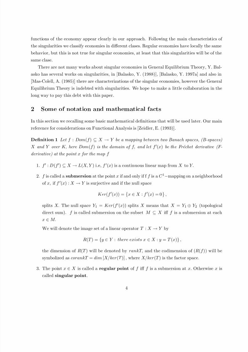
Definition 1 Let f : Dom(f ) ⊆ X → Y be a mapping between two Banach spaces, (B-spaces)
X and Y over K, here Dom(f ) is the domain of f, and let f (x) be the Frechet derivative (F-
derivative) at the point x for the map f
1. f : D(f ) ⊆ X → L(X, Y ) i.e, f (x) is a continuous linear map from X to Y.
2. f is called a submersion at the point x if and only if f f is a C 1−mapping on a neighborhood
of x, if f
(x) : X → Y is surjective and if the null space
Ker(f (x)) =
x ∈ X : f (x) = 0
,
splits X. The null space Y 1 = Ker(f (x)) splits X means that X = Y 1 ⊕ Y 2 (topological
direct sum). f is called submersion on the subset M ⊆ X iff f is a submersion at each
x ∈ M.
We will denote the image set of a linear operator T : X → Y by
R(T ) = y ∈ Y : there exists x ∈ X : y = T (x) ,
the dimension of R(T ) will be denoted by rankT, and the codimension of (R(f )) will be
symbolized as corankT = dim [X/ker(T )] , where X/ker(T ) is the factor space.
3. The point x ∈ X is called a regular point of f iff f is a submersion at x. Otherwise x is
called singular point.
4
7/27/2019 A Characterization of Infinity Dimensional Walrasian Economies
http://slidepdf.com/reader/full/a-characterization-of-infinity-dimensional-walrasian-economies 5/25
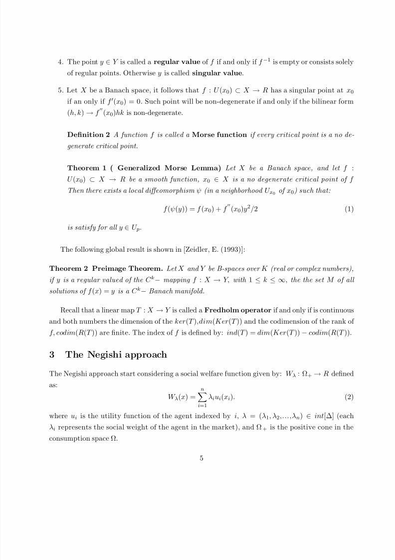
4. The point y ∈ Y is called a regular value of f if and only if f −1 is empty or consists solely
of regular points. Otherwise y is called singular value.
5. Let X be a Banach space, it follows that f : U (x0) ⊂ X → R has a singular point at x0
if an only if f (x0) = 0. Such point will be non-degenerate if and only if the bilinear form
(h, k) → f
(x0)hk is non-degenerate.
Definition 2 A function f is called a Morse function if every critical point is a no de-
generate critical point.
Theorem 1 ( Generalized Morse Lemma) Let X be a Banach space, and let f :
U (x0) ⊂ X → R be a smooth function, x0 ∈ X is a no degenerate critical point of f
Then there exists a local diffeomorphism ψ (in a neighborhood U x0 of x0) such that:
f (ψ(y)) = f (x0) + f
(x0)y2/2 (1)
is satisfy for all y ∈ U p.
The following global result is shown in [Zeidler, E. (1993)]:
Theorem 2 Preimage Theorem. Let X and Y be B-spaces over K (real or complex numbers),
if y is a regular valued of the C k− mapping f : X → Y, with 1 ≤ k ≤ ∞, the the set M of all
solutions of f (x) = y is a C
k
− Banach manifold.
Recall that a linear map T : X → Y is called a Fredholm operator if and only if is continuous
and both numbers the dimension of the ker(T ),dim(Ker(T )) and the codimension of the rank of
f, codim(R(T )) are finite. The index of f is defined by: ind(T ) = dim(Ker(T )) − codim(R(T )).
3 The Negishi approach
The Negishi approach start considering a social welfare function given by: W λ : Ω+ → R defined
as:
W λ(x) =ni=1
λiui(xi). (2)
where ui is the utility function of the agent indexed by i, λ = (λ1, λ2,...,λn) ∈ int[∆] (each
λi represents the social weight of the agent in the market), and Ω+ is the positive cone in the
consumption space Ω.
5

7/27/2019 A Characterization of Infinity Dimensional Walrasian Economies
http://slidepdf.com/reader/full/a-characterization-of-infinity-dimensional-walrasian-economies 6/25
As it is well know if x∗ ∈ Ω solves the maximization problem of W λ∗(x) for a given λ∗, subject
to be a factible allocation i.e.,
x∗ ∈ F = x ∈ Ω+ :n
i=1
xi ≤n
i=1
withen x∗ is a Pareto optimal allocation . Reciprocally it can be proved that if a factible al-
location x∗, is Pareto optimal, then there exists any λ∗ ∈ ∆ such that x∗, maximize W λ∗ ,
see [Accinelli, E. (1996)] There exists some Pareto optimal allocation where x∗i = 0 for some
i ∈ 1, 2,...,n, if each agent has positive no null endowments, these cases are possible if and only
if the agents indexed in this subset be out of the market, i.e., if and only if λi = 0. Then we can
restrict ourselves, without loss of generality, to consider only cases where λ ∈ ∆+.
In this way characterized the set of Pareto optimal allocations, our next step is to choose the
elements x∗ in the Pareto optimal set such that can be supported by a price p and satisfying
px∗ = pwi for all i = 1, 2,...,n i.e., an equilibrium allocation.
Suppose that the aggregate endowment of the economy is fixed, call it W, son
i=1 = w. We
will use the following notation
For any λ ∈ int [∆] = λ ∈ ∆ : λi > 0 ∀i ∈ I ,
x(λ, W ) = argmax
ni=1
λiui(x), s.tni=1
xi =ni=1
wi
. (3)
and let e : ∆ × Ω → Rn be the excess utility function, which coordinates are given by:
ei(λ, W ) = ui(xi(λ, W ))(xi(λ, W )) − wi).
Here ui(xi(λ, W )) : X → R is the F-differential of the utility ui(xi(λ, W )).
Definition 3 For fixed utility functions, for each w ∈ Ω we define the set
E q (w) = λ ∈ ∆+ : ew(λ) = 0 ,
it will be called the set of the Equilibrium Social Weights.
In [Accinelli, E. (1996)] is show that the equilibrium social weights is a non-empty set.
Theorem 3 Let λ ∈ E q (w), and let x∗(λ) be a factible allocation, solution of the maximization
problem of W λ and let γ (λ) be the corresponding vector of Lagrange multipliers. Then, the pair (x∗(λ), γ (λ)) is a walrasian equilibrium and reciprocally, if ( p, x) is a walrasian equilibrium then,
there exists λ ∈ E q such that x maximize W λ restricted to the factible allocations set, and p will
be the corresponding vector of Lagrange multipliers i.e., p = γ (λ).
The proof can be see in [Accinelli, E. (1996)].
6

7/27/2019 A Characterization of Infinity Dimensional Walrasian Economies
http://slidepdf.com/reader/full/a-characterization-of-infinity-dimensional-walrasian-economies 7/25
4 The equilibrium set as a Banach manifold
The first order conditions for (3) are ;
λiu
i(xi(λ, W ))) = λhu
h(xh(λ, W )), ∀h = ini=1 xi(λ, w) = W, (4)
where W =n
i=1 wi. It follows that for each i, the consumption of the i-agent, given by the
function xi : ∆ × Ω → X is, for all λ ∈ int[∆] and w ∈ Ω, a F-differentiable function. We denote
by xi,λj(λ, W ) and xi,wj (λ, W ) de partial F-derivatives with respect to the variable λ j and w j
respectively, j ∈ 1, 2,...,n.
The following are well know properties of the excess utility function:
(1) λe(λ, w) = 0.
2) e(αλ,w) = e(λ, w), ∀α > 0.
See for instance [Accinelli, E. (1996)].
From item (1) it follows that the rank of the jacobian matrix J λe(·, w) of the excess utility
function e(·, w) : ∆ → Rn is at most equal to n − 1. And as from item (2) we know that if
ei(λ, w) = 0 ∀i = 1, 2,...,n − 1, then en(λ, w) = 0, we will consider the restricted function
e : ∆ × Ω → Rn−1. This is the restricted function obtained from the excess utility function
removing one of its coordinates.
The following theorem holds:
Theorem 4 If the positve cone of the consumption space, has a non-empty interior then, there exists an open and dense subset Ω0 ⊆ Ω such that
E q/Ω0 = (λ, w) ∈ int[∆] × Ω0 : e(λ, w) = 0
is a Banach manifold.
Proof: To prove this theorem, we will prove the following assertions:
(i) There exist a residual set Ω0 ⊆ Ω such that, the mapping e : int[∆] × Ω0 → Rn−1 is C 1,
and zero is a regular value of e i.e. for all (λ, w) ∈ int[∆] × Ω0, such that e(λ, w) = 0 the
mapping e is a submersion.
(ii) For each parameter w ∈ Ω0, the mapping e(·, w) : int[∆] → Rn−1 is Fredholm of index zero.
(iii) Convergence of e(λn, wn) → 0 as n → ∞ and convergence of wn implies the existence of
a convergent subsequence of λn in int[∆].
7

7/27/2019 A Characterization of Infinity Dimensional Walrasian Economies
http://slidepdf.com/reader/full/a-characterization-of-infinity-dimensional-walrasian-economies 8/25
• Now, from [Zeidler, E. (1993)] section (4.19), the theorem follows.
Proof of the step (i): Consider the mapping from int[∆] × Ω0 → Rn−1 defined by the formula:
λ, w → e(λ, w),
where e(λ, w) is the vector (in Rn−1) defined by n − 1 coordinates of the vector e(λ, w).
We need to prove that 0 is a regular value of the restricted excess utility function e. So the
restricted excess utility function e is a submersion at each point (λ, w) ∈ λ × Ω, i.e, e(λ, w) :
int[∆] × Ω0 → Rn−1 is surjective and the null space Ker(e(λ, w)) splits X.
To be true that e is a submersion all that is required is that the linear tangent mapping is
always onto, or equivalently that the rank of the linear map e will be always equal to n − 1.
The existence of ∂xi∂wj
and ∂xi∂λh
is a consequence of the first order conditions (4) and the hy-
pothesis on the utility functions.The F-derivative of e(λ, ·) can be write as:
∂ (e1, e2, . . . , en−1)
∂ (w1, w2, . . . wn)= (5)
e1∂x1∂w1
e1∂x1∂w2
. . . e1∂x1∂wn
e2∂x2∂w1
e2∂x2∂w2
. . . e2∂x2∂wn
......
......
en−1∂xn−1∂w1
en−1∂xn−1∂w2
. . . en−1∂xn−1∂wn
−
u1 0 . . . 00 u2 . . . 0...
......
...0 0 . . . un−1
Where ek(λ, w) = uk(xk(λ, W )) [xk(λ, W ) − wk] − uk(xk(λ, W ).
We will prove that this matrix has rank n − 1. To see this suppose that we consider a little
change in endowment given by w(v) = w + v, where v = (v1, v2,...,vn) ∈ Rn is a vector in a
small open neighborhood U of zero, such that vn =n−1
i=1 vi. The vector v will be thought as a
state-independent parameter for redistributions of initial endowments. Observe thatn
i=1 wi(v) =ni=1 wi = W.
The excess utility function for the economy E (v) = ui, w(v)i will be:
e(λ, v) = (e1(λ, v1),...,en(λ, vn)) , (6)
where
ei(λ, v) = ui(xi(λ, W ))[xi(λ, W ) − wi − vi].
Observe that the allocations that solve (3) for the economies E (v) and E are the same.
It is easy to see that:
8
7/27/2019 A Characterization of Infinity Dimensional Walrasian Economies
http://slidepdf.com/reader/full/a-characterization-of-infinity-dimensional-walrasian-economies 9/25
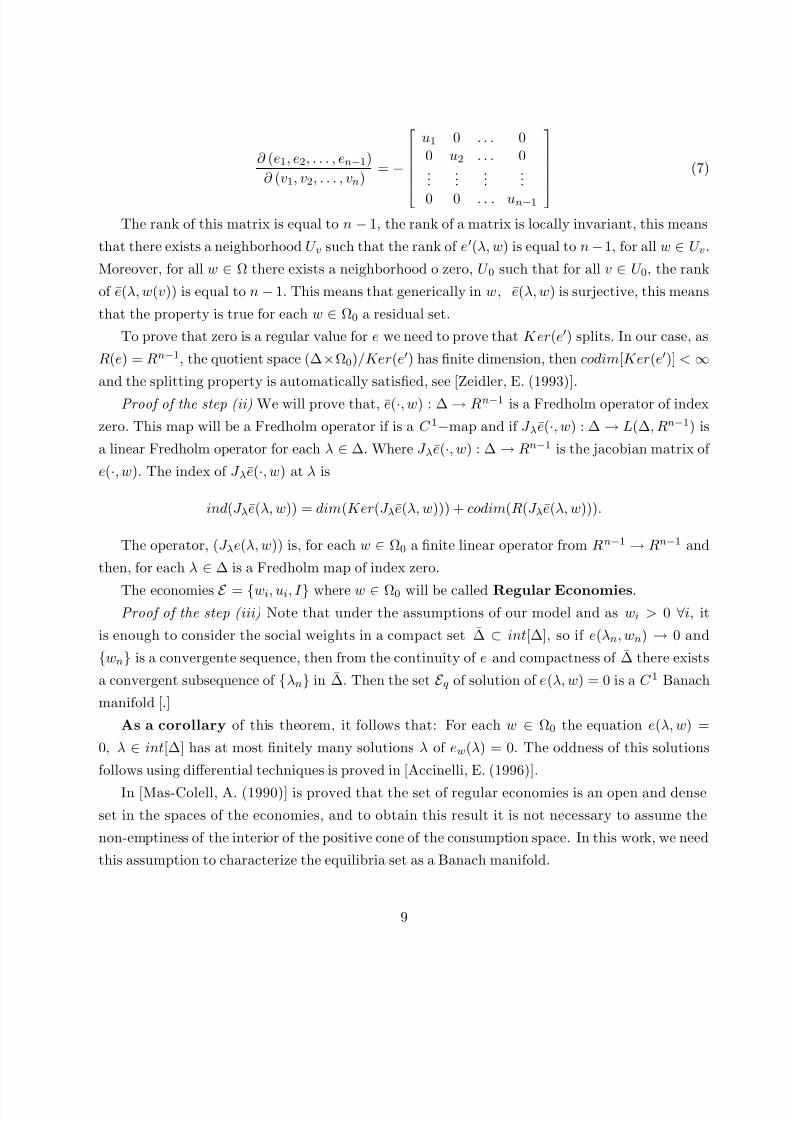
∂ (e1, e2, . . . , en−1)
∂ (v1, v2, . . . , vn)= −
u1 0 . . . 00 u2 . . . 0...
......
...
0 0 . . . un−1
(7)
The rank of this matrix is equal to n − 1, the rank of a matrix is locally invariant, this means
that there exists a neighborhood U v such that the rank of e(λ, w) is equal to n − 1, for all w ∈ U v.
Moreover, for all w ∈ Ω there exists a neighborhood o zero, U 0 such that for all v ∈ U 0, the rank
of e(λ, w(v)) is equal to n − 1. This means that generically in w, e(λ, w) is surjective, this means
that the property is true for each w ∈ Ω0 a residual set.
To prove that zero is a regular value for e we need to prove that Ker(e) splits. In our case, as
R(e) = Rn−1, the quotient space (∆×Ω0)/Ker(e) has finite dimension, then codim[Ker(e)] < ∞
and the splitting property is automatically satisfied, see [Zeidler, E. (1993)].
Proof of the step (ii) We will prove that, e(·, w) : ∆ → Rn−1 is a Fredholm operator of index
zero. This map will be a Fredholm operator if is a C 1−map and if J λe(·, w) : ∆ → L(∆, Rn−1) is
a linear Fredholm operator for each λ ∈ ∆. Where J λe(·, w) : ∆ → Rn−1 is the jacobian matrix of
e(·, w). The index of J λe(·, w) at λ is
ind(J λe(λ, w)) = dim(Ker(J λe(λ, w))) + codim(R(J λe(λ, w))).
The operator, (J λe(λ, w)) is, for each w ∈ Ω0 a finite linear operator from Rn−1 → Rn−1 and
then, for each λ ∈ ∆ is a Fredholm map of index zero.
The economies E = wi, ui, I where w ∈ Ω0 will be called Regular Economies.Proof of the step (iii) Note that under the assumptions of our model and as wi > 0 ∀i, it
is enough to consider the social weights in a compact set ∆ ⊂ int[∆], so if e(λn, wn) → 0 and
wn is a convergente sequence, then from the continuity of e and compactness of ∆ there exists
a convergent subsequence of λn in ∆. Then the set E q of solution of e(λ, w) = 0 is a C 1 Banach
manifold [.]
As a corollary of this theorem, it follows that: For each w ∈ Ω0 the equation e(λ, w) =
0, λ ∈ int[∆] has at most finitely many solutions λ of ew(λ) = 0. The oddness of this solutions
follows using differential techniques is proved in [Accinelli, E. (1996)].
In [Mas-Colell, A. (1990)] is proved that the set of regular economies is an open and dense
set in the spaces of the economies, and to obtain this result it is not necessary to assume the
non-emptiness of the interior of the positive cone of the consumption space. In this work, we need
this assumption to characterize the equilibria set as a Banach manifold.
9

7/27/2019 A Characterization of Infinity Dimensional Walrasian Economies
http://slidepdf.com/reader/full/a-characterization-of-infinity-dimensional-walrasian-economies 10/25
5 Singular economies and its properties
In this section utility functions are fixed and we describe each economy by its excess utility
function e : int[∆] × Ω → Rn−1. The equilibria of an economy are described by the state variables
λ = (λ1, λ2,...,λn), ∈ E q (w) these equilibrium states change when the parameters w ∈ Ω change,
these parameters are called external or control parameters. Given w the set of λ such that
e(λ, w) = ew(λ) = 0 determine the state of the system, i.e. the equilibrium in which the system
rest. The parameters w describe the dependence of the system on external forces, the action of
these forces cause changes in the states of the economy. Generically these changes are no so big,
and the new state is similar to the previous one, this is because generically economies are regular.
Nevertheless in some cases, a sudden transition resulting from a continuous parameter change,
can be shown. This kind of changes is referred to as a catastrophe. A catastrophe can take place
only in a neighborhood of a singular economy.A state, or equilibrium λ ∈ E q (w) such that the corank of the jacobian matrix J λew is positive,
will be called singular or critical equilibrium. Singular economies will be classified in two big
classes:
Definition 4 The set of singular economies such that:
1. for all λ ∈ E q (w) the corankJ λew(λ) ≤ 1 and with strict inequality for at least one λ ∈
E q (w) This is the set of no degenerate singular economies. And the states of equilibria
corresponding will be called critical no degenerate equilibria.
2. And the set of all remain singular economies, it will will be called the set of degeneratesingular economies. An equilibrium λ ∈ E q (w) where corankJ λew(λ) > 1, will be called
a degenerate critical equilibrium.
The corank of J λew(λ) is given by:
corankJ λew(λ)
= (n − 1) − dim
J λew(λ)
.
In this way we can say that the corank is a measure for the degree of the degeneration of the
equilibria.
To clarify these considerations and to justify the introduction to the Catastrophe Theory in
economics, let us now consider the following two examples:
Example 1 Let E(W) = ui, wi; i = 1, 2 be the set of interchange economies which total endow-
ment W = (W 1, W 2) are fixed. This means that:
W j = w1 j + w2 j, j = 1, 2; (∗)
10

7/27/2019 A Characterization of Infinity Dimensional Walrasian Economies
http://slidepdf.com/reader/full/a-characterization-of-infinity-dimensional-walrasian-economies 11/25
where wij is the initial endowment of agent i in the commodity j. Initial endowment may be
redistributed but the total endowment can not be modified, so the components of W are constants.
The equilibrium set will be symbolized by:
V W = (λ, w) ∈ int[∆] × Ω, : e(λ, w) = 0, w1 j + w2 j = W j ; j = 1, 2
An equilibrium is a pair (λ, w) such that e1(λ, w) = 0, e2(λ, w) = 0. As in this example the
total supply is fixed, to characterize the equilibrium, we can consider, without loss of generality
the initial endowments of the only one agent, for instance the agent indexed by 1. And from the
fact that social weight are in the sphere of radius 1, it is enough to consider only one component
of λ. So, a pair (λ, w) will be an equilibrium if and only if, e1(λ1; w11, w12) = 0.
Suppose that the excess utility function of the agent 1 is given by:
e1(λ1, w11, w12) = 3W 1λ1 − 3w11(λ1)1
3 + w12. (8)
In terms of catastrophe theory λ1 is the state variable and w1 are the control parameters.
The social equilibria of this economy will be given by the set of pairs (λ, w) such that its compo-
nents (λ1, w11, w12) solve the equation e1(λ1, w11, w12) = 0 and by the corresponding (λ2, w21, w22)
obtained from the former. The set
C F = (λ1, w11, w12) ∈ V W : detJ λ1e1(λ1, w11, w12) = 0,
is the Catastrophe surface.
The economies whose endowments are in this surface are the singular economies. In our case
this surface is defined by:
C F =
(λ1, w11, w12) ∈ V W :
∂e
∂λ1= 3W 1 − w11λ−
2
3 = 0
.
Explicitly:
C F =
w11
3W 1
3
2
, w11,2w
3
2
11
(3W 1)1
2
.
The projection of this set in the space of parameters will be called the Bifurcation set. In
our case:
BF =
w11,
2w3
2
11
(3W 1)1
2
.
This set is represented in the space of parameters, w11, w12 by a parabola. By varying the
parameters continuously, and crossing this parabola, something unusual happens: the number of
11

7/27/2019 A Characterization of Infinity Dimensional Walrasian Economies
http://slidepdf.com/reader/full/a-characterization-of-infinity-dimensional-walrasian-economies 12/25
possible states of equilibria associated with the initial endowments w change: increases or decreases
by two.
The number of equilibria is given by the sign of δ where:
δ = 27
w11
W 1
2
− 4
w12
W 1
3
so if:
• δ < 0 associate with w, there exist three regular equilibria.
• δ > 0 there is one regular equilibrium associate with w.
• δ = 0, w11w22 = 0 there exists one critical (or singular) equilibrium and one regular equi-
librium.
The additional consideration taken from [ Balasko, Y. 1997b]: the set of regular economies with
a unique equilibrium is arc connected in the two agents case, help us to obtain a good geometric
representation of economies. Therefore, the set of economies where δ > 0 is an arc-connected set.
The hessian matrix of the considerate excess utility function (the matrix defined by the second
order derivatives of ew at λ) is singular, this means, as we will see later, that the critical equilib-
rium is degenerate. So economies with endowments which satisfy δ = 0 are degenerate singular
economies.
Example 2 Consider the economy E = uα,i, wi, R+l, i = 1, 2 which utility functions are:
uα,1 = x11 − 1α
x−α12uα,2 = x21 − 1
αx−α21 x22
,
and endowments W = w1 + w2.
Following the Negishi approach we begin solving the optimization problem:
maxW λ(x) = λ1u1(x1) + λ2u2(x2),
restricted to the factible set:. F = x ∈ R4
+
: 2i=1
xi ≤ 2i=1
wiDenoting λ1 = λ it follows that λ2 = 1 − λ. Then we write the excess utility function:
euw =
1−λλ
α1+α −
1−λλ
1
1+α − w12
1−λλ
+ w21
1−λλ
−α1+α −
1−λλ
−11+α − w21
1−λλ
−1+ w12
12
7/27/2019 A Characterization of Infinity Dimensional Walrasian Economies
http://slidepdf.com/reader/full/a-characterization-of-infinity-dimensional-walrasian-economies 13/25
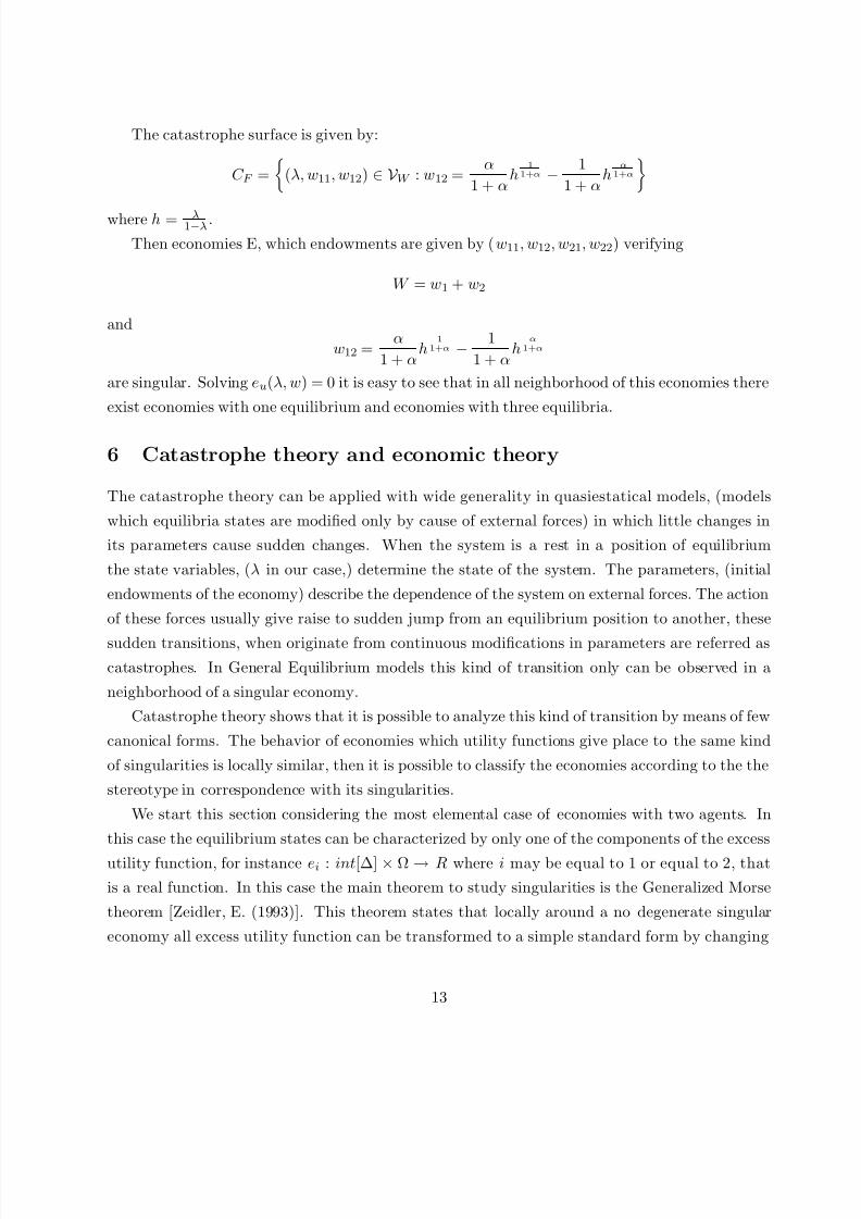
The catastrophe surface is given by:
C F =
(λ, w11, w12) ∈ V W : w12 =
α
1 + αh
1
1+α −1
1 + αh
α1+α
where h = λ1−λ .
Then economies E, which endowments are given by (w11, w12, w21, w22) verifying
W = w1 + w2
and
w12 =α
1 + αh
1
1+α −1
1 + αh
α1+α
are singular. Solving eu(λ, w) = 0 it is easy to see that in all neighborhood of this economies there
exist economies with one equilibrium and economies with three equilibria.
6 Catastrophe theory and economic theory
The catastrophe theory can be applied with wide generality in quasiestatical models, (models
which equilibria states are modified only by cause of external forces) in which little changes in
its parameters cause sudden changes. When the system is a rest in a position of equilibrium
the state variables, (λ in our case,) determine the state of the system. The parameters, (initial
endowments of the economy) describe the dependence of the system on external forces. The action
of these forces usually give raise to sudden jump from an equilibrium position to another, these
sudden transitions, when originate from continuous modifications in parameters are referred as
catastrophes. In General Equilibrium models this kind of transition only can be observed in a
neighborhood of a singular economy.
Catastrophe theory shows that it is possible to analyze this kind of transition by means of few
canonical forms. The behavior of economies which utility functions give place to the same kind
of singularities is locally similar, then it is possible to classify the economies according to the the
stereotype in correspondence with its singularities.
We start this section considering the most elemental case of economies with two agents. In
this case the equilibrium states can be characterized by only one of the components of the excess
utility function, for instance ei : int[∆] × Ω → R where i may be equal to 1 or equal to 2, that
is a real function. In this case the main theorem to study singularities is the Generalized Morse
theorem [Zeidler, E. (1993)]. This theorem states that locally around a no degenerate singular
economy all excess utility function can be transformed to a simple standard form by changing
13
7/27/2019 A Characterization of Infinity Dimensional Walrasian Economies
http://slidepdf.com/reader/full/a-characterization-of-infinity-dimensional-walrasian-economies 14/25
coordinates. There are exactly 3 such forms and these are quadratic forms. To each function
corresponds exactly one of these canonical forms.
Later more general cases will be considered.
6.1 Two agents economies
Let E = ui, wi; i = 1, 2 be an interchange economy with two agents and l commodities. The
property 2 of definition 4, allow us to characterize the economy by one component of its excess
utility function as a function of the initial endowments, and property 1 of the same definition,
allow us consider only one of the two social weight. Let ei : (0, 1) × Ω → R be the excess utility
function of the agent indexed by i. The function is defined by (λi, w) → ei(λi, w).
The characterization of no degenerates critical points in terms of the hessian matrix (see section
(2))is a confortable condition to characterize singular economies:
Remark 1 A two agents interchange economy w, is a degenerate singular economy if and only if
the hessian matrix of ewi :
∂ewi =
∂ewi(λ)
∂λhλk
, h, k = 1, 2..., n.
is singular for at least one λ ∈ E q (w).
The significance of Morse’s Lemma is in reducing the family of all smooth functions vanishing
at the origin (f ( p) = 0) in Rn with the origin as a no degenerate critical point, to just n + 1 simple
stereotypes.Applying this theorem in economic setting it follows that, in a neighborhood U λ of a social
equilibrium λ of a no degenerate singular economy w, the excess utilities functions ew will behave
in similar way for every non degenerate w with independence of utilities. Moreover, if given the
utility function, there are only no degenerates singular economies, then by smooth coordinate
transformation it is possible to reduce the family of all excess utility function to just 3 simple
stereotypes, namely:
ewi(ψ(λ)) = ±λ21 ± λ2
2.
The following two theorems, help us to know some characteristics of the no degenerates singular
economies
Theorem 5 Let f : X → R be a smooth function with a no degenerate critical point p. Then
there exists a neighborhood V of p in X such that no other critical point of f are in V, i. e., no
degenerate critical points are isolates.
14

7/27/2019 A Characterization of Infinity Dimensional Walrasian Economies
http://slidepdf.com/reader/full/a-characterization-of-infinity-dimensional-walrasian-economies 15/25
So, no degenerate critical points are isolates, and if we considere endowments in a finite subset
of Ω there are finite number of they. Moreover, generically in Ω, there exists only one λ such that
ew(λ) = 0 is a critical no degenerate social equilibrium. This follows as a conclusion of the next
theorem:
Theorem 6 Let X be a smooth manifold. The set of Morse functions all of whose critical values
are distinct (i.e., if p and q are distinct critical points of f in X, then f ( p) = f (q )) form a residual
set in C ∞(X, R).
This means that generically, if the economy E = ui, wi, I is singular no degenerate, then
there exists only one critical equilibrium λ ∈ E q (w).
Remark 2 (About singularities and oddness in the number of equilibria) In terms of
the economic theory this means that, generically a singular no degenerate economy w, with 2 agents has only one critical equilibrium. The oddness of the number of equilibria force that in
a neighborhood of the singular economy there are economies w with only one λ ∈ E q (barw) and
economies ¯w with three distinct λ ∈ E q (w)
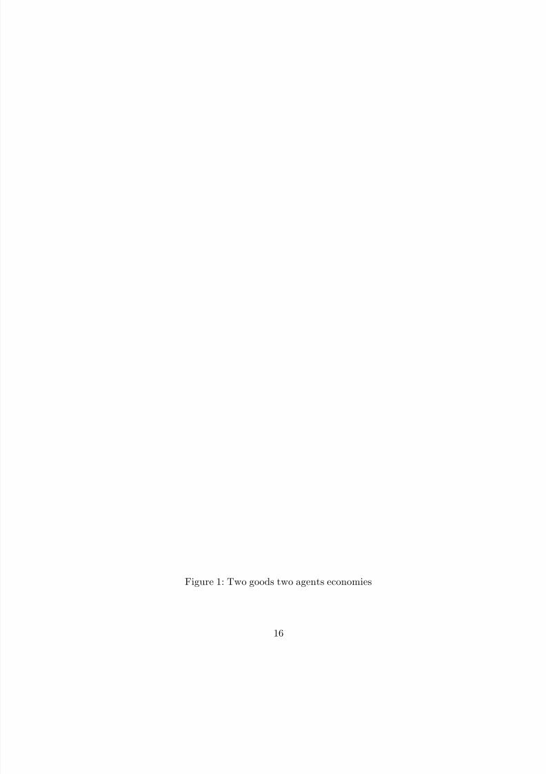
If we add the hypothesis of 2 commodities, the oddness and the arc-connectedness properties of
the regular economies with one equilibrium before mentioned, allows us to show the picture as
generically representative of the behavior of this kind of economies.
Finally, the economic interpretation of the above considerations is that:
1) Regular economies have a similar behavior around an equilibrium.
2) The excess utility function of all no degenerate singular economy with two agents, have a
similar behavior in a neighborhood of a no degenerate critical equilibrium. And this behavior
is characterized by a second order polinomial.
The following question is of major importance for a qualitative understanding of many eco-
nomical (in general scientific) phenomena: When does the Taylor expansion up to some order
k
j
k
xf (u) = f (x) + f (x)u + ... + f
k
u
k
/k!provide enough information to understand the local behavior of a function f at x? This means:
it would be possible to characterize the behavior of an economy for the Taylor expansion of the
excess utility function up to some order k? As we shown above, using the Morse lemma it is
possible for a no degenerate two-agent economies.
15
7/27/2019 A Characterization of Infinity Dimensional Walrasian Economies
http://slidepdf.com/reader/full/a-characterization-of-infinity-dimensional-walrasian-economies 16/25
Figure 1: Two goods two agents economies
16

7/27/2019 A Characterization of Infinity Dimensional Walrasian Economies
http://slidepdf.com/reader/full/a-characterization-of-infinity-dimensional-walrasian-economies 17/25
7 Starting a classification: The S r classification
We begin this section with an important question of the catastrophe hteory, the k-determination
of C k(X, Y )functions and then we will related this topic with the the qualitative behavior of the
economies in a neighborhood of an equilibrium. We consider economies with an arbitrary but
finite number of consumers and then we focus our attention on two kind of singularities: the
folds and the cusps. Finally we will connect the kind of the singularities that it can appear in a
particular economy with the number of agent and goods that this economy has.
The first question: The question of the k−determination of a function is fundamental to
catastrophe theory: when a function f is determined in a neighborhood of a point x by one of its
Taylor polynomials at x in the sense that every other function having the same Taylor polynomial
coincide with f in a neighborhood of x up to a diffeomorphism? Recall that a map f ∈ C k(X, Y ),
is k-equivalent at a point x0 ∈ X to a map g ∈ C
k
(U, V ) at a point u0 if and only if there existlocal C k diffeomorphisms at u0 and f (x0) respectively with φ(u0) = x0 and ψ(f (x0) = g(u0). In
this case f and g need only be defined in a neighborhood of x0 and u0. Where X,Y,U, and V are
Banach-manifolds. There is no obvious relationship between this two kind of equivalence.
Recall that a function cannot be determined by its Taylor polynomial in an arbitrary point
x. For instance the functions f : R2 → R, f (x, y) = x2, and g : R2 → R, g(x, y) = x2 − y2l,
have the same k−polynomial at 0 ∈ R2 when l > k/2 holds, but if if φ = (φ1, φ2) is any local
diffeomorphism at 0 ∈ R2 then:
f (φ(0, y)) = (φ1(0, y))2 = −y2l = g(0, y)
is true for nonzero y ∈ R Thus f is not determined by any of its Taylor polynomials.
Definition 5 We will say that the economy E = ui, wi, i ∈ I is k-equivalent at a λ0 ∈ E q (w) to
the economy E = ui, wi, i ∈ I at λ1 ∈ E q (w) if and only if its respective excess utility functions
ew and ew are k − equivalent functions at λ0 and λ1 .
1. Let f : U ( p) ⊂ X → Y be C k(X, Y ), k ≥ 1 and X and Y Banach manifolds and let g = j1k(f )
i.e.,
g(u) = f (x) + f (x)u
If f is submersion or inmersion at x then f is k−equivalent to g at 0.
2. If X = Rn and Y = Rm and f is a submersion at x then f is k-equivalent at x to g at 0.
Moreover, if rankf (x) = r, then f is k-equivalent at x to h : X → Y with
h(x1,...,xn) = (x1,...,xr, 0...0)
17

7/27/2019 A Characterization of Infinity Dimensional Walrasian Economies
http://slidepdf.com/reader/full/a-characterization-of-infinity-dimensional-walrasian-economies 18/25
This means that the excess utility function of all regular economy is k−determined, i.e, locally,
in a neighborhood of an equilibrium, they have the same qualitative behavior.
A function f : U (x) ⊂ X → Rm is called k− determined if and only if for each function
g : U (x) ⊂ X → Rm
with the same Taylor polinomial of degree kjk
pf, there exists a local C ∞
diffeomorphism φ ∈ Rn such that g(φ(u)) = jkxf (u) in a neighborhood of x.
Roughly speaking, a function f will be k-determined if all function which differ from f only
in terms of order higher than k behave qualitatively like the k − th Taylor polinomial of f. This
means that the Taylor expansion up to order k completely determines f and its perturbations
with terms of order higher than k. So, if the excess utility function of a given economy, ew is
k-determined, then all economy wich excess utility function have the same Taylor polinomial up
to order k, show the same qualitative behavior than the former.
We will look at what is called the k − jet of that function at p ∈ Dom(f ), and then we will
show some characteristic of the set of singularities of each clase of functions identified in this way.
Definition 6 Jet Bundles: Let X and Y be n and m dimensional, smooth manifolds and f, g :
X → Y, f (x) = g(x) = y be smooth functions. Consider the following equivalence relation: f ∼k g
will mean that the k − th Taylor expansion of f coincides with the k − th expansion of g at x. The
equivalence class of f at x under this relation is called the k-jet of f at x, and will be denoted
by J k(f )x.
• By the symbol Dhf we represent the set of partial derivatives such that: ∂ |h|f
∂xh11...∂x
hnn
where
|h| =n
j=1 h j, hi ≥ 0 i = 1, 2,...,n.
• Let J k(X, Y )x,y denote the set of equivalence classes under ∼k at p of mapping f : X → Y
where f (x) = y.
• An element σ ∈ J k(X, Y ) = ∪(x,y)∈X ×Y J k(X, Y )x,y, is called k-jet where f (x) = y.
• let J k(X, Y ) = ∪(x,y)∈X ×Y J k(X, Y )x,y (disjoint union). Then J k(X, Y ) is the set of all k-jet
with source X and target Y.
Theorem 7 Let X and Y be smooth manifolds with n = dimX and m = dimY. Then, J k(X, Y )
is a smooth manifold with:
dimJ k(X, Y ) = m + n + dim(Bkn,m),
where Bkn,m is the space of formed by the direct sum of polynomial in n−variables with degree ≤ k.
18

7/27/2019 A Characterization of Infinity Dimensional Walrasian Economies
http://slidepdf.com/reader/full/a-characterization-of-infinity-dimensional-walrasian-economies 19/25
The object of our analysis is the excess utility function, and the social equilibria. Obviously its
critical values can be other than zero, but our interest is focused at the origin, because only this
value have an economical means: The preimagen of zero by e is the set of the social equilibria.
Then we are interested in consider the class J k
(X, Y )(λ,w),0 that is, the k− jet σ with source(λ, w) ∈ X = int[∆] × Ω and target 0 ∈ Y = Rn−1.
Remark 3 (Notation) To avoid future possible mistakes arose from the notation, from now on
we will represent the jacobian matrix of a mapping f at p by the symbol: (∂f )x.
Let σ ∈ J 1(X, Y ); then σ defines a unique linear mapping of T xX → T yY, where x is the
source of σ and y is the target of σ. Let f be a representative of σ in C ∞(X, Y ). Then (∂f )x
is that linear mapping. Define rank(σ) = rank(∂f ) p and corank(σ) = µ − rankσ, where µ =
min(dimX, dimY ). Let
S r =
σ ∈ J 1(X, Y ) : corank(σ) = r
.
This is the subset of the equivalence classes under ∼1 in C ∞(X, Y ) such that the corank(∂f ) p = r
where p is the source of σ. The subset S r is a submanifold of J 1(X, Y ) with
codim S r = (n − µ + r)(m − µ + r),
see [Golubistki, M. and Guillemin,V.(1973)].
As we said above our interest is the class σ ∈ J 1(int[∆] × Ω, Rn−1) with source (λ, w) and
target 0 ∈ Y = Rn−1. It follows that: dimX = (n − 1) + nl and dimY = n − 1, then µ = n − 1.
So, codimS r = (nl + r)r.
The set of singularities of f : X → Y where the rank of it jacobian matrix drops by r
i.e., the set x ∈ X where rank(∂f )x = min(dimX, dimY ) − r is represented by the symbol:
S r(f ) = ( j1f )−1(S r). Then S r(f ) will be, generically, a manifold of the same codimension that
(S r), [Golubistki, M. and Guillemin,V.(1973)].
As codimS r(f ) = dimX − dimS r(f ) ≥ 0 there is a relation between the kind of singularities
possible for each f ∈ C ∞(X, Y ) and the dimension of the manifold.
Applying this concepts to economics, S r(e) is the set of critical points of e where the jacobian
matrix of e drops rank by r. This set is a manifold and the set of critical social equilibria is the
subset of (λ, w) ∈ S r(e) : e(λ, w) = 0. For instance, S 1(e) is the set of no degenerate critical social
equilibria that is, the set of pairs (λ, w) ∈ int[∆] × Ω such that e(λ, w) = 0.
It follows that, there exists a relation between the number of agents and commodities and the
form of possible singularities. In others words, the excess utility function could have only some
19

7/27/2019 A Characterization of Infinity Dimensional Walrasian Economies
http://slidepdf.com/reader/full/a-characterization-of-infinity-dimensional-walrasian-economies 20/25
types of singularities, and these will be determined by the number of commodities and consumer
in the economy, to be more precise, the codimension of S r depend on the number of goods and
agents, and its dimension depend only on the agent number but do no depend on the number of
goods.Then, codimS r(f ) > |dimX − dimY |, then dimS r(f ) < dimY. Applying this observation to
economics, where: X = int[∆] × Ω, Y = Rn−1 and f is the excess utility function e, it follows
that: if n is the number of consumers of the economy then, dimS r(e) < n − 1. In cases where
n = 2 we obtain that singular economies are generically isolates points in Ω.
It is important to remind that the topology used in theorems about transversality of maps
in C ∞(X, Y ) is the Withney topology, this is a very strong topology, therefore if a proposition
is satisfy generically in a topological space with the Whitney topology, is indeed satisfy in quite
large sense and is a strong result.
The next example clarify these considerations:
Example 3 If the economy have two goods and two consumers we have that dimX = 5, dimY =
1 and codimS r = (4 + r)r so, e could have only singularities of kind S 1 and S 0. Note that if r = 1
we obtain that critical social equilibria are isolate points.
Now we will show some characteristic of S 1 singularities:
7.1 The Fold and the Cusp in economics
Definition 7 (Submersions with Folds) Let X and Y be a smooth manifolds with dimX ≥
dimY Let f : X → Y be a smooth mapping, such that J 1f is transversal to S 1. Then a point
p ∈ S 1(f ) is called fold point if:
T xS 1(f ) + Ker(∂f )x = T xX.
Definition 8 We say that a map is one generic if J 1f is transversal to S 1. This is a generic
situation. [Golubistki, M. and Guillemin,V.(1973)].
Where S 1 is the submanifold of J 1(X, Y ) of jets of corank 1, then S 1(f ) = ( j1f )−1(S 1) is a
submanifold of X with codimS 1(f ) = codim(S 1) = k + 1 where k = dimX − dimY. Note that isx ∈ S 1(f ) then dimKer(∂f )x = k + 1. That is, the tangent space to S 1(f ) and the kernel of (∂f )x
have complementary dimensions.
Therefore, codimS 1(e) = nl +1 it follows that if (λ, w) ∈ S 1(e) then, dimKer(∂e)(λ,w) = nl + 1
where n is the number of agents and l the number of commodities.
20

7/27/2019 A Characterization of Infinity Dimensional Walrasian Economies
http://slidepdf.com/reader/full/a-characterization-of-infinity-dimensional-walrasian-economies 21/25
The next theorem characterize the local behavior of a submersion with folds near a fold, similar
to the Morse theorem for real function. (Recall that if X and Y are manifolds, and f : X → Y is
differentiable mapping, with rank(∂f ) p the maximum possible, is a submersion if dimX ≥ dimY.)
Theorem 8 Let f : X → Y be a submersion with folds and let p be in S 1(f ). Then there exist
coordinates x1, x2,...,xn centered at x0 and y1, y2,...yn centered at f ( p) so that in these coordinates
f is given by:
(x1, x2,...,xn) → (x1, x2,...,xm−1, x2m ± ... ± x2n)
This theorem is proved in [Golubistki, M. and Guillemin,V.(1973)].
Taking a particularly simple example of 2-manifolds (manifolds with dimension equal 2), we
see the reason for the nomenclature fold point. In this case the normal form is given by: (x1, x2) →
(x1, x22). This transformation is obtained by means of the following steps:
1) Map the (x1, x2) map onto the parabolic cylinder, (x1, x2, x22),
2) then, project onto the (x1, x3) plane.
An example: 3-agent economies:
Let X and Y be 2-manifolds and let f : X → Y be a one generic mapping. By our computation
codimS 1(f ) = 1 in X , and S 2 does not occur, since it would to have codimension 4. Let p be a
point in S 1(f ) and q = f ( p). One of the following two situations can occur:
(a) T pS 1(f ) ⊕ Ker(∂f ) p = T pX.
(b) T pS 1(f ) = Ker(∂f ) p
Remark 4 Whitney proved that if f belongs to C ∞(X, Y ) generically the only singularities are
folds and simple cusp.
Note that only if the interchange economy has 3 agents and fixed initial endowment the excess
utility function is a mapping between 2-manifolds, ew : int[∆] → R2.
Let λ = (λ1, λ2, λ3) ∈ ∆ be a singular social equilibrium for the economy w.
i) In the first case (item (a)) applying 8 one can choose a system of coordinates ( λ1, λ2)
centered at (λ1, λ2) ∈ S 1(ew) and (e1, e2) centered at ew(λ) = 0 such that ew is a fold:
(λ1, λ2) → (λ1, λ22).
21

7/27/2019 A Characterization of Infinity Dimensional Walrasian Economies
http://slidepdf.com/reader/full/a-characterization-of-infinity-dimensional-walrasian-economies 22/25
ii) If (b) holds the situation is considerable more complicated. Generically singularities, in this
case, are simple cusps. In this case one can find coordinates (λ1, λ2) centered at e(λ) such
that:
(¯λ1,
¯λ2) → (
¯λ1,
¯λ1
¯λ2 +
¯λ3
2).
In a neighborhood of a cusp or a fold there exist regular economies with different number of
equilibrium. Recall that, at the moment of through a singularity the changes in the number of
equilibria appear.
7.2 The S r,s singularities
Let f : X → Y be one generic. We will denote by S r,s(f ) the set of points where the map
f : S r(f ) → Y drops by rank s. Analogous to the S r it si possible to build:
S r,s ⊂ σ ∈ J 2(X, Y ) : corank(σ) = r.
Note that x ∈ S r,s(f ) if and only if x ∈ S r(f ) and the kernel of (∂f )x intersects the tangent
space to S r(f ) in a subspace a s dimensional subspace. From dimS r(e) < n − 1 it follows that in
cases of economies where n = 2 the singularities are S 1,0(e) folds, or S 1,1(e) cusps.
Using the Transversality Theorem in [Golubistki, M. and Guillemin,V.(1973)] is proved that
j2f is generically transversal to S r,s and then the sets S r,s are submanifolds in J 2(X, Y ) and like
in the case of S r(f ),
S r,s(f ) = ( j2(f ))−1(S r,s).
In the cited work the dimension of S r,s(f ) is computed.
Generically S r,s(f ) are submanifolds in X whose dimensions are given by:
dimS r,s(f ) = dimX − r2 − µr − (codimS r,s(f ) in S r(f )) . (9)
where
codimS r,s =m
2x(k + 1) −
m
2(k − s)(k − s + 1) − s(k − s), (10)
where
• m = dimY − dimX + k
• k = r + max(dimX − dimY, 0).
[Golubistki, M. and Guillemin,V.(1973)]
22

7/27/2019 A Characterization of Infinity Dimensional Walrasian Economies
http://slidepdf.com/reader/full/a-characterization-of-infinity-dimensional-walrasian-economies 23/25
In this way we see that the set of possible singularities in economics are strongly relate with
the number of agents and commodities, then it follows that some kind of singularities appear only
if the number of agents are big enough.
7.3 Singularities and its relations with the dimension of the economy
Applying to economies with a finite number of agents and commodities, we obtain that:
• k = r + nl and m = r
• where n is the number of agents, l is the number of commodities an r is the codimension of
(∂e) in the singularity.
So, generically, we obtain substituting in (10) that:
codimS r,s(e) = (r + nl) (rs − s) − rs2
+ rs2
− rs22
+ s2.
Substituting k = nl + r in (10) it follows:
codimS r,s(e) = nl (rs − s) + r2s −rs2
2+
rs
2+ s2.
From (9) we obtain that
dimS r,s(e) = nl (1 − r − rs + s) + (n − 1) + rs
−r +
s
2−
1
2
− s2 − r2.
In particular for S 1,1 it follows that codimS 11 = 2 and dimS 11 = n − 2 holds.
From (9) and (10) it follows that generically, singularities likeS 1,2(e) only could appear if the
number of consumer is n > 4, because n > 4 is a necessary condition to be dimS 1,2(e) ≥ 0
8 Conclusions
The introduction of the excess utility function in equilibrium analysis allow us to work in infinite
dimensional economies in a similar way than in finite dimensional models and, on the other hand,
to improve our understanding of the way in which equilibria depend upon economic parameters
(initial endowments) and shows the strong relation existing between utilities and the behavior of the economic system.
This function reflects the weight of consumers in the markets, and show the changes in their
relative weights when the initial endowments change. Near a regular economy these changes
are smooth and there is not qualitative changes, but around a singularity sudden and big changes
23
7/27/2019 A Characterization of Infinity Dimensional Walrasian Economies
http://slidepdf.com/reader/full/a-characterization-of-infinity-dimensional-walrasian-economies 24/25
occur. The economic weight of the agents change drastically, overthrowing the existent order. The
uncertainty in the behavior of the economy is a direct result of the existence of singular economies.
If there would not be singularities, economics would be a science with perfect prediction, without
sense and perfectly boredNevertheless, most part of the literature in economics have focused on regular economies
whose equilibria change smoothly according to the changes in the endowments. The study of the
discontinuous behavior requires to consider singularities, this led us to the catastrophe theory. This
theory refers to drastic changes, however to be sudden, abrupt and unexpected the catastrophe
theory show that these changes have a similar substratum that allows us to do a classification
according its geometric representation. So, the study of singularities require catastrophe theory
and the theory of mapping and their singularities, in this way one might have an approximation
to understanding the forms of the unexpected changes in economics.
A final consideration: The excess utility function allows us to extend the analysis of singulari-ties for economies with finite dimensional consumption spaces, to infinite dimensional economies.
Then also in these cases, the catastrophe theory may be a gate to begin to understand the behavior
of an economical system with infinitely many goods in a neighborhood of a singularity.
24

7/27/2019 A Characterization of Infinity Dimensional Walrasian Economies
http://slidepdf.com/reader/full/a-characterization-of-infinity-dimensional-walrasian-economies 25/25
References
[Accinelli, E. (1996)] “Existence and Uniqueness of the Equilibrium for Infinite Dimensional
Economies”.Revista de Estudios Econ´ omicos; Universidad de Chile .
[ Aliprantis, C.D; Brown, D.J.; Burkinshaw, O.] Existence and Optimality of Competitive Equi-
librium. Springer-Verlag, 1990.
[Araujo, A. (1987)] “The Non-Existence of Smooth Demand in General Banach spaces”. Journal
of Mathematical Economics 17, 1-11
[Arnold, V.; Varchenko, A.; Goussein-Zade, S.] “Singularites des Applications Differeentiables”
Editions Mir, 1982 .
[Balasko, Y. (1988)] “Foundations of the Theory of General Equilibrium”. Academic Press, inc.
[Balasko, Y. 1997a] Equilibrium Analysis of the Infinite Horizont Models wit Smooth Discounted
Utility Functions. Journal of Economics Dynamics and Control 21 783-829.
[ Balasko, Y. 1997b] The Natural Projection Approach to the Infinite Horizont Models. Journal
of Mathematical Economics 27 251-265.
[Castrigiano, D.; Hayes, S.] Catastrophe Theory . Adisson-Wesley. 1993.
[Chichilnisky, G. and Zhou, Y.] Smooth Infinte Economies.Journal of Mathematica Economies
29, (1988) 27 - 42.
[Golubistki, M. and Guillemin,V.(1973)] “Stable Mappings and Their Singularities”. Springer
Verlag.
[Mas-Colell, A. (1985)] “The Theory of General Equilibrium, A Differentiable Approach”. Cam-
bridge University Press.
[Mas-Colell, A. (1990)] “Indeterminaci in Incomplete Market Economies.” Economic Theory 1
[Milnor, J. (1965)] “Topology from the Differential Viewpoint”. University of Virginia Press:
Charlottesville.
[Thom, R. (1962)] “Sur la Theorie des Enveloppes”.Journal de Mathematiques, XLI.
[Zeidler, E. (1993)] “Non Linear Functional Analysis and its Applications”(1). Springer Verlag.
25
Top Related