


Languages
Pages
Legal


ORIGINAL ARTICLE
5-Lumps kinetic modeling, simulation and optimizationfor hydrotreating of atmospheric crude oil residue
Sameer A. Esmaeel1 • Saba A. Gheni2 • Aysar T. Jarullah1
Received: 30 June 2015 / Accepted: 24 November 2015 / Published online: 17 December 2015
� The Author(s) 2015. This article is published with open access at Springerlink.com
Abstract This research aims at developing a discrete
kinetic model of the hydrotreating process of a crude oil
residue based on experiments. Thus, various experiments
were conducted in a continuous flow trickle bed reactor
over a temperature range of 653–693 K, liquid hourly
space velocity of 0.3–1.0 h-1, and hydrogen pressure of
6.0–10.0 MPas at a constant hydrogen to oil ratio of
1000 L L-1. The reduced crude residue had been assumed
to have five lumps: naphtha, kerosene, light gas oil, heavy
gas oil and vacuum residue. An optimization technique
based on the minimization of the sum of the squared error
between the experimental and predicted compositions of
the distillate fractions was used to calculate the optimal
value of kinetic parameters. The predicted product com-
position showed good agreement with the experimental
data for a wide range of operating conditions with a sum of
square errors of less than 5 %.
Keywords Atmospheric residue � Hydrotreating (HDT) �Trickle bed reactor (TBR) � Lumping model
List of symbols
T Temperature (K)
rA Rate of reaction (wt% h-1)
E Activation energy (kJ mol-1)
k Reaction rate constant [(wt%)1-n h-1]
A Frequency factor [(wt%)1-n h-1]
P Pressure (Pas)
P� Pressure reference (Pas)
LHSV Liquid hourly space velocity (h-1)
s Residence time (h)
rR Consumption rate of residue (wtR% h-1)
rHGO Consumption rate of heavy gasoil (wtHGO% h-1)
rLGO Reaction rate of light gasoil (wtLGO% h-1)
rK Reaction rate of kerosene (wtK% h-1)
rN Reaction rate of naphtha (wtN% h-1)
kR Reaction rate constant of residue [(wtR%)1-n h-1]
kHGO Reaction rate constant of heavy gasoil [(wtHGO%)1-n h-1]
kLGO Reaction rate constant of light gasoil
[(wtLGO%)1-n h-1]
kK Reaction rate constant of kerosene
[(wtK%)1-n h-1]
kN Reaction rate constant of naphtha
[(wtN%)1-n h-1]
n Reaction order (–)
m Deactivation rate order (–)
kd Deactivation rate constant (h-1)
yR Composition of residue fraction (wt%)
yHGO Composition of heavy gasoil fraction (wt%)
yLGO Composition of light gasoil fraction (wt%)
yK Composition of kerosene fraction (wt%)
yN Composition of naphtha fraction (wt%)
Greek symbols
U Catalyst activity
b Order of pressure term in modified Arrhenius equation
Symbols and abbreviations
R Residue
HGO Heavy gas oil
LGO Light gas oil
K Kerosene
& Saba A. Gheni
1 Chemical Engineering Department, Tikrit University, Tikrit,
Iraq
2 Chemical Engineering Department, University of Missouri,
Columbia, USA
123
Appl Petrochem Res (2016) 6:117–133
DOI 10.1007/s13203-015-0142-x

N Naphtha
HDT Hydrotreating
Introduction
The upgrading of heavy crude oil residues to more
valuable light and middle distillates is becoming
increasingly important for the global refining industry
because of the decline in conventional, light crude oil
sources [1]. The hydrogenolysis is defined as the trans-
formation of large hydrocarbon molecules (high boiling
point) into smaller molecules (low boiling point) in the
presence of hydrogen. In residue hydrotreatment, this
transformation occurs due to the breaking of carbon–
carbon bonds or the removal of large atoms that is
bonded to two unconnected pieces of hydrocarbon and
has been used as one of the techniques for the upgrading
of crude residues. For most of hydrotreating catalysts,
the conversion rate is primarily a function of operating
temperature, pressure and liquid hourly space velocity
(LHSV) [2]. It is generally used to process heavy oil
cuts. The process is tailored to various needs of
refineries to maximize middle distillates, gasoline, LPG
and similar products [3]. Kinetic model has a significant
effect on process optimization, unit design and catalyst
selection. Mathematical models for a trickle bed catalytic
reactor can be complex due to many microscopic and
macroscopic effects occurring inside the reactor, includ-
ing flow patterns of both phases, size and shape of a
catalyst particle, wetting of the catalyst pores with liquid
phase, pressure drop, intraparticle gradients, thermal
effects and, of course, kinetics on the catalyst surface
[4]. Laxminarasimhan et al. [5] described a five-param-
eter continuous model for hydrocracking of heavy pet-
roleum feedstocks that was subsequently used by
Khorasheh et al. [6, 7] and Ashouri et al. [8] to describe
the kinetics of hydrocracking, HDS, and HDN processes
of bitumen. Today, there are two types of kinetic models
available, detailed molecular models and lumped empir-
ical models. The detailed molecular model is very
accurate because it takes into account all possible reac-
tions and mechanisms. Although the predictive power of
detailed molecular models is much better than that of
lumped empirical models, but their application to heavy
feedstocks is very rare due to the complexity of the
mixture. However, the available analytical techniques are
incapable to identify the detailed molecular level of
heavy feedstocks [9]. There are other types of modeling
used to determine reactor performance such as hybrid
modeling which is a first-principles model (FPM) based
on the pseudo-component approach coupled with neural
network(s) in different hybrid architectures [10], Com-
bination of Genetic Algorithm and Sequential Quadratic
Programming which based on genetic algorithm and
sequential quadratic programming to determine the sig-
nificant reactions and their corresponding rate constants
[11], and some used kinetics to extract information about
yield [12] and other model of hydrocracking reactor [13].
The lumped kinetic models are commonly used in
modeling the hydrocracking of heavy feedstocks such as
atmospheric vacuum resides. The lumped kinetic models
have been classified into two types: discrete lumped
models and continues lumped models. Specifying the
chemical reactions involved in residual hydrocracking
and the actual composition of the products is a compli-
cated task. Therefore, the liquid product of residual
upgrading is normally divided into several product lumps
that are based on true boiling point temperature [14].
This is one approach to simplify the problem which
considers the partition of the components into a few
equivalent classes called lumps or lumping technique,
and then assume each class as an independent entity
[15]. The accuracy and the predictive power of discrete
lumping models mainly depend on the number of lumps.
As the amount of lumps increases, the predicted accu-
racy improves. Increasing the number of lumps, however,
will complicate the model by increasing the number of
model parameters [16]. Although numerous researchers
published about lumping model for some oils and resi-
dues [3, 17–21], there is a lack of models for predicting
kinetic parameters of atmospheric crude oil residue with
a flexibility of operating pressure along with the absence
of experimental data. The proposed model will estimate
the optimal conditions of the five lumps, naphtha, ker-
osene, light gasoil, heavy gasoil and lowest residue with
low content of impurities.
Experimental work
Feedstock (reduced crude oil)
The feedstock used in this study is an atmospheric crude
residue (RCR) derived from Kirkuk crude oil as a crude
model. It was obtained from the North Refineries Company
in Iraq. The physical properties of the feedstock are illus-
trated in Table 1, which are tested in North Refineries
Company laboratories.
Hydrogen gas
Hydrogen gas, 99.999 % purity, has been used for
hydrotreating of RCR.
118 Appl Petrochem Res (2016) 6:117–133
123

Catalyst
The catalyst used in this study is a Ni–Mo supported on
alumina that is a monofunctional catalyst and commonly
used for HDT of heavy residue such as atmospheric resi-
due. The specifications of catalyst are listed in Table 2.
Apparatus
The experiments of this study were conducted in an
experimental scale, high temperature, and high-pressure
trickle bed reactor (TBR). Process flow diagram of this
system is presented in Fig. 1. The continuous
hydrotreating of RCR is carried out in the TBR where
the feedstock and air pass through the reactor in co-
currently flow mode. The trickle bed reactor consists of a
316 stainless steel tubular reactor, 77 cm long, 1.5 cm
internal diameter, and controlled automatically by four
sections of 15-cm-high steel-jacket heaters. The first part
of length (30–35 % vol.) was packed with inert particles.
The second section (40 % vol.) contained a packing of
Ni–Mo catalyst. The bottom section was also packed
with inert particles of length (30–35 % vol.) to serve as
disengaging section [22]. To ensure isothermal operation,
the reactor had been heated, readings of temperature
increase versus time were recorded and a good perfor-
mance had been observed. Pre-RCR is stored in a 0.5 m3
feed tank with a coil heater connected to the tank that
raise RCR temperature to 100 �C to maintain a liquid
phase and avoid freezing. The feed tank is connected to a
high-pressure dosing pump that can dispense flow rates
from 0.0 to 0.07 mm3 min-1. Hydrogen flows from a
high-pressure cylinder (15 MPa) equipped with a pressure
controller to maintain constant operating pressure. The
gas flow meter is coupled with a high-precision valve,
which is used to control gas flow rate. The streams of
hydrogen and RCR flow to separate electrical heaters
(pre-heaters). The RCR and hydrogen gas streams are
mixed and then introduced to the reactor at the required
temperature when RCR is hydrotreated to the proposed
products. The outlet from the reactor flows through a
heat exchanger to a high-pressure gas–liquid separator to
separate excess hydrogen from the petroleum products
and H2S from liquid product, which is withdrawn from
sample points when reaction reaches the steady state.
Table 3 shows the description and specifications of TBR
unit and its constituents Fig. 2 shows the factors affect
the operation of trickle bed reactor.
Table 1 The properties of feedstock (RCR)
Specification Value
Specific gravity at 15.6 �C 0.9552
API 16.6
Flash point 95
Pour point ?15
Viscosity @ 50 �C/cst 223.1
Viscosity @ 100 �C/cst 22.6
Sulfur content 3.7 %
Distillation Vol.% (D1160)
Vol.% Temperature (�C)
IBP 335
5 352
10 375
20 428
30 458
40 495
50 543
60 562
70 587
Table 2 Properties of (Ni–Mo/alumina) catalyst
Value
Chemical specification
Ni 12
Mo 6
SiO2 1.2
Fe 0.67
Na2O 0.42
Al2O3 Balance
Physical specification
Form Extrude
Bulk density (g cm-3) 2.74
Mean particle diameter (mm) 6.4
Surface area (m2 g-1) 936
Fig. 1 Process flow diagram of trickle bed reactor unit
Appl Petrochem Res (2016) 6:117–133 119
123

Experimental procedure
Operating conditions
The major effect of operational variables employed in TBR
unit and their influence on the reactor performance can be
summarized as follows. To improve the dibenzothiophene
conversion, three procedures can be chosen: increase of
temperature (653–693 K), decrease of liquid hour space
velocity LHSV (0.3–1 h-1) and increase of pressure
(6–10 MPa) at a constant hydrogen to oil ratio (1000) over
nickel–molybdenum (Ni–Mo//c-Al2O3).
Experimental runs
The hydrotreating experiments were carried out in a
continuous isothermal trickle bed reactor packed with
40 % Ni–Mo//c-Al2O3 of the catalyst particles. The model
reduced crude oil is Kirkuk crude oil which is obtained
from the North Refineries Company, Iraq. The cooling
water is flowing through the heat exchanger and the
temperature of the cooling jackets is maintained below
293 K to prevent vaporization of light components present
in reduced crude and nitrogen gas is flown through the
system to check leaks and to get rid of any remaining
gases and liquid from the previous run. Reduced crude oil
mixed with hydrogen is flown through the reactor at 0.2
MPas pressure and temperature controller is set to the
feed injection temperature (it is lower than steady-state
operating temperature). When the temperature of air
reaches feed injection temperature the dosing pump is
turned on to allow a certain reduced crude oil flow rate
and the temperature is raised at the rate of 293 K h-1
until the steady-state temperature is reached. At the end of
a run, the RCR dosing pump is turned off keeping air gas
flow on to back wash any remaining light gas oil. Finally,
the air valve is closed and nitrogen is passed through the
system to remove the remaining air and to get the system
ready for the next run.
Laboratory tests
There are many tests in this work, the analysis tests of
products can be divided into two types, one for gas product
and the other for liquid product. The primary tests of
hydrotreating products revealed insignificant gases con-
centration of less than 0.124 % (a constant concentration,
selectivity, of the products gases have been observed dur-
ing experimentations). Thus, all the products analyzed and
modeled in this study are liquids. The tests applied to the
products of this work are as following:
Table 3 Experimental device description and specifications
Description Specification
Feed tank (containing
RCR)
Box, 0.008 m3
Compressor 13 MPa
Pre-heater Electrical coil
Pump Dosapro Milton Roy/Italy
Max flow = 0.00127 m3 h-1
Max. pressure = 12 MPa
Trickle bed reactor(TBR) Stainless steel 310
1.6 cm 9 73 cm
Control box Control box
Reactor heating jacket Electrical coils
Heat exchanger (cooler) Shell and tube (four tubes) stainless
steel
Separator Stainless steel
Pressure gauge Neu-tec/Italy
0–12.5 MPas
Gas flow meter Yamamoto
0–0.006 m3/min
Cooling water 293 K
Fig. 2 Variables affect operation of trickle bed reactor for hydroc-
racking of RCR
120 Appl Petrochem Res (2016) 6:117–133
123

True boiling point distillation Feed and products are
distillated by ASTM D1160 Vacuum Distillation Appara-
tus for distillation of petroleum products.
Sulfur content Feed and products sulfur content are tested
by ASTM D2622 (X-RAY Spectrometer ARL OPTIM’X
from Thermo Scientific). This test method provides rapid
measurement of total sulfur in petroleum and petroleum
products with a minimum of sample preparation. A typical
analysis time is 1–2 min per sample.
Mathematical model of TBR for hydrotreatingreaction
Process model is very profitable and is utilized for operator
training, safety systems design, design of operation and oper-
ational control systems designs. The improvement of faster
computer and sophisticated numerical methods has enabled
modeling and solution of the whole operation [23]. Many
authors have reported that pore diffusion effects can be taken
into account within the framework of an effective or apparent
reaction rate constant (i.e., multiplying intrinsic reaction rate
constant by effectiveness factor), in order to formulate a
pseudo homogeneous basic plug flow model which is suffi-
cient to describe the progress of chemical reactions in the
liquid phase of a TBR [24–26]. The required data and available
tools with the assumptions for modeling and simulation pro-
cesses RCR hydrotreating are tabulated in Fig. 3.
Discrete lumping model
In this study, we considered the conversion of atmospheric
residue to generate five product lumps that are characterized
by various true boiling point temperature (TBP) range. In this
respect, the five fractions are: naphtha (N), kerosene (K), light
gas oil (LGO), heavy gas oil (HGO) and vacuum residue (VR).
The boiling ranges of these fractions are given in Table 4. The
vacuum residue in these lumps represents the amount of
unconverted feed while the naphtha, kerosene, light and heavy
gas oil are complex mixtures of hydrocarbons that have
resulted from conversion. Naphtha fraction is poorly generated
in residue hydro-processing. Kerosene is a highly demanded
fraction due to demand for kerosene as a domestic heating
fuel. The gas oil fractions are an important cut that is mainly
used for the production of transportation fuels. The vacuum
residue fraction has a very low demand and it is known for its
deteriorating effects on the catalyst of downstream processes
such as fluid catalytic cracking. Figure 3 illustrates reaction
pathways with weight fraction. Note if all pathways of reac-
tions were considered, the model would include twenty-one
kinetic parameters. All these parameters should be estimated
from experimental data, and it was too laborious.
Kinetic model
Due to the complexity of mathematical models for a trickle
bed catalytic reactor, it is more practical to reduce the
complexity of the reactor, focusing only on momentous
process variables. This suggests a development of simpler
models that incorporates less number of parameters. For
each reaction, a kinetic expression (R) is formulated as a
function of mass concentration (C) and kinetic parameters
(k0, E). The following assumptions have been made in the
development of the present model:
1. Modified Arrhenius equation applied for each reaction.
2. Hydrotreating is a first-order hydrotreating reaction.
Since hydrogen is present in excess, the rate of
hydrotreating can be considered independent of hydro-
gen concentration [27].
3. The reactor operates under isothermal condition.Fig. 3 General expectation of reaction pathways of RCR
hydrocracking
Table 4 True boiling range of the lumps
Fractions TBP range (�C)
Naphtha (N) IBP–433
Kerosene (K) 433–528
Light gas oil (LGO) 528–618
Heavy gas oil (HGO) 618–813
Vacuum residue (VR) >813
Appl Petrochem Res (2016) 6:117–133 121
123

4. The trickle bed reactor follows a plug flow pattern. Axial
dispersion, external and internal gradients are neglected.
5. The feed gas, hydrogen, is pure.
6. The petroleum feed and the products are in liquid
phase in the reactor.
7. The experimental unit is working under steady-state
operation.
Based on these assumptions, the kinetic constants of the
proposed model are:
Residue (F):
kFj ¼ ukoFj exp�EFj
RT
� �P
PO
� �b
ð1Þ
Note: j in Eq. 1 represents heavy gas oil (HGO), light
gas oil (LGO), kerosene (K) and naphtha (N) lumps.
Heavy gasoil (HGO):
kHGOj0 ¼ ukoHGOj0exp�EHGOj0
RT
� �P
PO
� �b
ð2Þ
where j0 represents light gas oil (LGO), kerosene (K) and
naphtha (N) lumps.
Light gasoil (LGO):
kLGOj00 ¼ ukoLGOj00 exp�ELGOj00
RT
� �P
PO
� �b
ð3Þ
where j00 are kerosene (K) and naphtha (N) lumps.
Kerosene (K):
kKN ¼ ukoKN exp�EKN
RT
� �P
PO
� �b
ð4Þ
T and R are the absolute value of bed temperature and
ideal gas constant, respectively, and u represents the
deactivation rate, it is represented by:
u ¼ 1= 1þ kdtð Þm ð5Þ
The reaction rates (R) can be formulated as follows:
RF ¼XN
j¼HGO
kF:jyF ð6Þ
Heavy gasoil (RHGO):
RHGO ¼ kF:HGOyF �XN
j¼LGO
kHGOjyHGO ð7Þ
Light gasoil (RLGO):
RLGO ¼ kF:LGOyF þ kHGO:LGOyHGO �XNj¼K
kLGO:jyLGO ð8Þ
Kerosene (RK):RK ¼ kF:KyF þ kHGO:KyHGO þ kLGO:KyLGO
�kK:NCN
ð9Þ
Naphtha (RN):
RK ¼ kF:KyF þ kHGO:KyHGO þ kLGO:KyLGO
+ kK:NCN
ð10Þ
The set of equations from 1 to 10 were coded and solved
simultaneously using the gPROMS [28].
Parameter estimation techniques
Parameter estimation is necessary in several fields of sci-
ence and engineering as many physiochemical processes
are described by systems equations with unown parame-
ters. Recently, the benefits of developing kinetic models for
chemical engineers with accurate parameter calculations
have increased owing to the developed control technolo-
gies and optimization of process, which can apply funda-
mental models [29]. Estimation of kinetic parameters is an
important and difficult step in the development of models,
but calculations of unknown kinetic parameters can be
achieved by utilizing experimental data and model-based
technique. When estimating kinetic parameters of the
models, the goal is to calculate appropriate parameter
values so that errors between experimental and theoretical
data (based on mathematical model) are minimized. On the
other hand, the predicted values from the model should
match the experimental data as closely as possible [29]. For
the purpose of process optimization, design of reactor and
process control, it is important to develop kinetic models
that can accurately predict the concentration of product
under process conditions.
The experimental data of hydrotreating reaction were
adjusted with a simple power law kinetic model. Plug flow
behavior was considered, and the reaction
dyi
ds¼ �kynj : ð11Þ
where yi is the yield weight fraction of i lump in reaction
products, s the residence time (s = 1/LHSV), k the global
rate constant, and n the reaction order of residue
hydrotreating.
Yields were determined by integration of Eq. 11, where
yio is the initial weight fraction of i lump in the feed:
ycalc:i ¼ y1�nio þ ks n� 1ð Þ
� �1= 1� nð Þ ð12Þ
For parameter estimation, the objective function, OBJ,
as given below, as minimized:
OBJ: ¼XNt
n¼1
Xnj¼F
wj ymeas:jn � y
prid:jn
� �2
: ð13Þ
where Nt is the number of test runs, yexpi is the weight
fraction measured experimentally of i lump and yestii is the
weight fraction estimated by the model of i lump, in the
122 Appl Petrochem Res (2016) 6:117–133
123

products. Reactions and expressions in Eqs. 1 through 13
were coded and solved simultaneously using General
PROcess Modeling System (gPROMS) programming
environment to evaluate the product yields (yi). According
to the initial suggestion of kinetic parameters from previ-
ous works, the composition of all fractions has been esti-
mated by application of model equations in gPROMS.
Optimization problem formulation
The optimization problem formulation for parameter esti-
mation can be stated as follows:
Given The reactor configuration, the feedstock, the
catalyst, reaction temperature, hydrogen pressure and liq-
uid hourly space velocity;
Obtained The reaction orders of cracking of residue,
HGO, LGO and kerosene (n1, n2, n3 and n4) and deacti-
vation rate order (m), reaction rate constants (ki) at dif-
ferent temperatures, pressures and LHSVs and deactivation
rate constant (kd) at different temperatures, pressure-de-
pendent parameter (b).So as to minimize The sum of square errors (SQE).
SQE ¼XNt
n¼1
XGj¼F
Wj � Ymeasjn � Y
predji
� �2 ð14Þ
In Eq. 14, Nt, Ymeasjn and Y
predjn are the numbers of test
runs, the measured product yield and the predicted one by
model, respectively
Subject to Process constraints and linear bounds on all
optimization variables in the process.
Mathematically, the problem can be presented as:
f(t, x(t), x*(t), u(t)) = 0 represents the process model,
where t is the independent variable (time), x(t) gives the set
of all differential and algebraic variables, x*(t) denotes
the derivative of differential variables with respect to time,
u(t) is the control variable. Initial and final time of reaction
is [t0, tf] and the function f is assumed to be continuously
differentiable with respect to all its arguments.
The optimization solution method used by gPROMS is a
two-step method known as a feasible path approach. The first
step performs the simulation to converge all the equality
constraints (described by f) and to satisfy the inequality
constraints. The second step performs the optimization (up-
dates the values of the decision variables such as the kinetic
parameters). The optimization problem is posed as a Non-
Linear Programming (NLP) problem and is solved using a
Successive Quadratic Programming (SQP) method within
gPROMS (see Jarullah et al. [30–32] for further details).
Results and discussion
Experimental results
Effect of catalyst on process conversion at operating
conditions
The effect of metal oxide loading, reaction temperature,
LHSV and initial concentration on the process conversion
Table 5 Hydrocracking results
LHSV Press. Temp. Naphtha Kero. LGO VGO VR
0.3 60 380 1.279 1.193 7.336 55.971 34.221
0.7 60 380 0.801 0.709 5.002 54.002 39.486
1 60 380 0.618 0.548 4.002 53.067 41.765
0.3 60 400 2.328 1.401 8.453 57.091 30.727
0.7 60 400 1.519 0.961 6.032 55.345 36.143
1 60 400 1.201 0.756 4.981 54.344 38.718
0.3 60 420 2.986 2.096 10.939 60.014 23.965
0.7 60 420 1.995 1.455 8.013 57.176 31.361
1 60 420 1.689 1.198 6.654 56.211 34.248
0.3 80 380 1.626 1.398 7.942 56.174 32.86
0.7 80 380 0.965 0.832 5.131 54.408 38.664
1 80 380 0.755 0.672 4.121 53.429 41.023
0.3 80 400 2.503 1.717 8.811 58.532 28.437
0.7 80 400 1.691 1.159 6.215 56.728 34.207
1 80 400 1.318 0.936 5.069 55.179 37.498
0.3 80 420 3.486 2.589 11.308 60.761 21.856
0.7 80 420 2.485 1.794 8.109 58.037 29.575
1 80 420 1.998 1.602 6.981 57.781 31.638
0.3 100 380 1.978 1.641 8.059 56.476 31.846
0.7 100 380 1.204 1.021 5.332 54.872 37.571
1 100 380 0.921 0.821 4.301 54.292 39.665
0.3 100 400 2.877 2.033 9.225 58.997 26.868
0.7 100 400 2.001 1.406 6.467 56.811 33.315
1 100 400 1.618 1.188 5.189 55.991 36.014
0.3 100 420 3.756 3.141 11.397 61.165 20.541
0.7 100 420 2.764 2.112 8.385 58.897 27.842
1 100 420 2.198 1.798 7.105 58.048 30.856
Min SSE
k; kd; n;m;b
s:t f t; x tð Þ; x� tð Þ;ðu tð ÞÞ ¼ 0 t0; tf
� � (model equality constraints)
kLij � kUij ½i ¼ 1; 2; 3; . . .10; j ¼ 0; 1; 2for each pressure�
Inequality constraints
kLd � kUd Inequality constraints
nL � nU Inequality constraints
mL �mU Inequality constraints
bL � bU Inequality constraints
Appl Petrochem Res (2016) 6:117–133 123
123
is investigated. The yields of naphtha (N) are normally very
low in residue hydrogenolysis. The kerosene (K) fraction is
normally the most significant hydrotreated products of the
residue hydrogenolysis. The gasoil fraction (GO) is an
important cut because it is used as a feedstock for fluid
catalytic cracking and hydrocracking, which are mainly
operated for the production of transportation fuels. The
demand for the vacuum residue (VR) is very low due to its
deteriorating effects on the downstream processes such as
fluid catalytic cracking (FCC). The atmospheric residue of
the model crude oil consists of no naphtha and kerosene,
0.527 wt% light gas oil, 51.345 and 48.128 wt%. Below
653 K high conversion has not been observed on the pro-
cesses. There was also no significant difference in con-
version for the hydrotreating of model RCR catalyzed by
temperature of 653 K and LHSV of 1 h-1. The optimal
results were obtained with a temperature of 693 K, LHSV
of 0.3 h-1 and 10 MPas. The results of experimental runs
are shown in Table 5.
As a result of studying fractions data listed in Table 5,
the domination of catalyst hydrotreating over thermal
cracking is confidently concluded. This conclusion is based
(a)
(b)
(c)
0102030405060708090
100
370 380 390 400 410 420 430
Wt %
Temperature. (C)
VRVGOLGOKERO.NAPHTHA
0102030405060708090
100
370 380 390 400 410 420 430
Wt %
Temperature. (C)
VRVGOLGOKERO.NAPHTHA
0102030405060708090
100
370 380 390 400 410 420 430
Wt %
Temperature. (C)
VRVGOLGOKERO.NAPHTHA
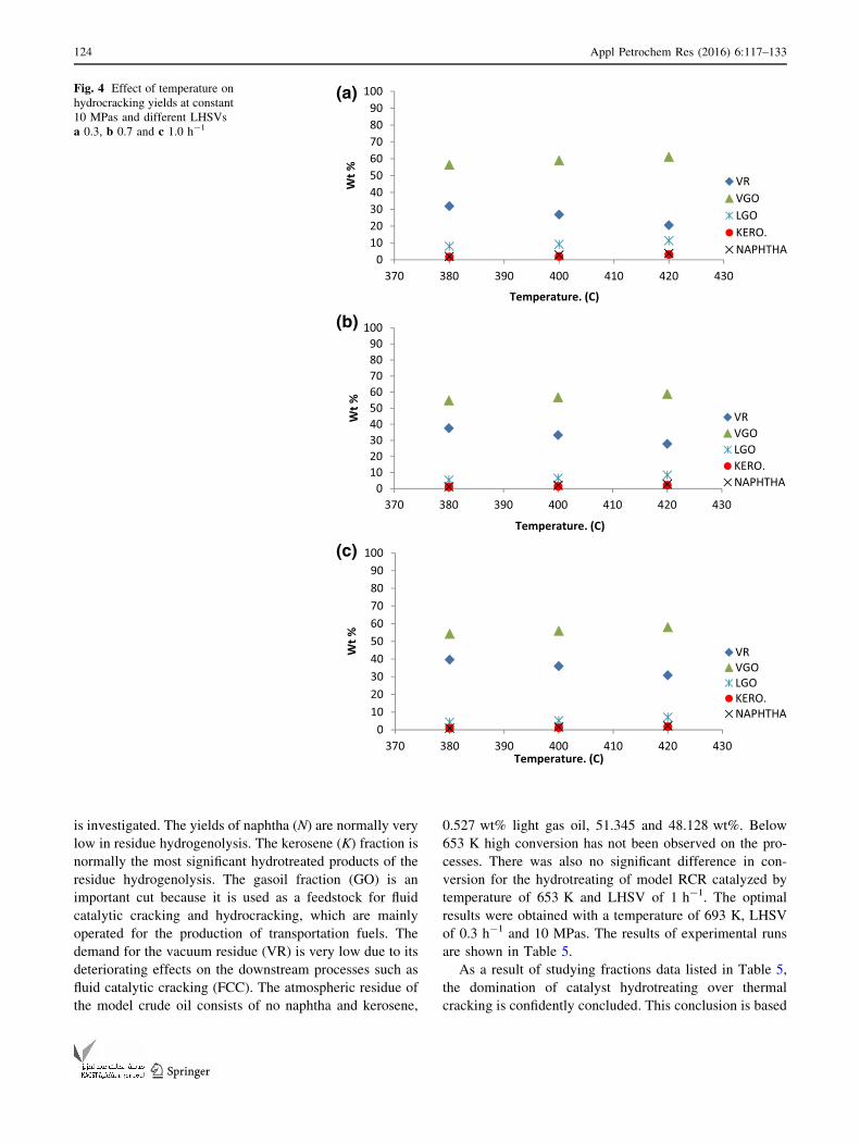
Fig. 4 Effect of temperature on
hydrocracking yields at constant
10 MPas and different LHSVs
a 0.3, b 0.7 and c 1.0 h-1
124 Appl Petrochem Res (2016) 6:117–133
123

on two main observations. The first one is the suppression
of gas formation, while the second observation is the
selectivity towards kerosene formation. It is known that
thermal cracking yields huge amounts of light products and
gases. On the contrary, experimental data revealed that
very low concentration of naphtha were obtained. Table 5
shows that the highest concentration of naphtha fraction is
3.756 wt%. This concentration was achieved at the highest
severity. Another indication of catalytic domination is the
selectivity toward kerosene and light gasoil production, this
selectivity has resulted from the high concentration of
molybdenum in the catalyst [33].
Effect of temperature on process conversion
The hydrotreating reactivity of RCRwas also investigated at
different temperatures (653–693 K, and different LHSV
(0.3–1 h-1), in the presence of the (Ni–Mo/c-Al2O3) cata-
lyst. The effects of LHSV and temperature on hydrogenol-
ysis reactions are shown in Fig. 4. At low temperature, the
conversion of RCR was very low, then increased gradually
with increasing reaction temperature from 653 to 693 K. The
yield of naphtha and kerosene was decreased by increasing
the LHSV which agreed with the role of the smaller the
LHSV, the better the hydrotreating [34]. The role of
Fig. 5 Effect of LHSV on
hydrocracking yields at constant
pressure at 10 MPas bar and
different temperatures a 380,
b 400 and c 420 �C
Appl Petrochem Res (2016) 6:117–133 125
123

temperature was routine, for naphtha and kerosene the
temperature stimulates the hydrogenolysis reactions, so that
the yield of both was improved.
By increasing the temperature, the rate of cracking of
feed and the products will increase. Because of this, the
increase in temperature leads to further cracking for gasoil
and kerosene toward the formation of smaller fractions
(naphtha and kerosene). The presence of the catalyst pro-
vides selectivity toward kerosene formation even at high
temperatures, but also very high temperatures are
undesirable in an industrial scale because of the problems
of deactivation of the catalyst.
Effect of LHSV on process conversion
The effect of LHSV on hydrogenolysis yields is presented
in Fig. 5. It can be seen, increasing LHSV has an adverse
impact on RCR cracking. Figure 5 depicts the effect of
liquid flow rate on RCR cracking. As clearly noted from
this figure, a high yield of light fraction is obtained at
Fig. 6 Effect of pressure on
hydrocracking yields at constant
temperature at 420 �C and
different LHSVs a 0.3, b 0.7
and c 1.0 h-1
126 Appl Petrochem Res (2016) 6:117–133
123

LHSV = 0.3 h-1. Note, at LHSV of 0.7 and 1 h-1, the
yield was lower. Actually, increasing liquid flow rate
reduces the residence time of the reactant thus reducing
reaction time of RCR with hydrogen (gas reactant).
Moreover, higher liquid flow rate gives greater liquid
holdup, which evidently decreases the contact of liquid and
gas reactants at the catalyst active site, by increasing film
thickness. Figure 5 also illustrates that the yield of naphtha
and kerosene was decreased by increasing the LHSV which
was in agreement with the role of the residence time—the
smaller the LHSV, the better the hydrotreating [3]. The
small difference in conversion between LHSV = 0.3 and
LHSV = 1 is attributed to the effect on hydrogen con-
sumption. The hydrogen consumption increased sharply
with temperature, but LHSV does not have any sensible
variation on it. The hydrogen consumption is a little higher
at lower LHSVs (LHSV less than 1).
Effect of pressure on process conversion
The effect of pressure on hydrogenolysis yields is pre-
sented in Fig. 6. It can be seen, increasing pressure has a
significant impact on RCR cracking. The effect of pressure
Table 6 Optimal model parameters obtained by optimization process
Parameter Value Units
n1 1.1662 (–)
n2 1.9892 (–)
n3 1.9936 (–)
n4 1.023 (–)
m 0.4207 (–)
kd1 1.4448 h-1
kd2 3.6917 h-1
kd3 6.8324 h-1
b 0.0177 (–)
Table 7 Comparison between experimental product composition and
predicted product composition of atmospheric residue (RCR)
LHSV Press. Temp. Predicted Experimental Error%
0.3 60 380 33.944 34.221 0.809
0.7 60 380 41.333 39.486 4.677
1 60 380 43.246 41.765 3.546
0.3 60 400 33.377 30.727 8.624
0.7 60 400 41.025 36.143 13.507
1 60 400 43.019 38.718 11.108
0.3 60 420 31.851 23.965 32.906
0.7 60 420 40.18 31.361 28.121
1 60 420 42.392 34.248 23.779
0.3 80 380 30.502 32.86 7.176
0.7 80 380 39.41 38.664 1.929
1 80 380 41.816 41.023 1.933
0.3 80 400 24.088 28.437 15.293
0.7 80 400 35.412 34.207 3.522
1 80 400 38.763 37.498 3.373
0.3 80 420 28.463 21.856 30.229
0.7 80 420 38.204 29.575 29.176
1 80 420 40.906 31.638 29.294
0.3 100 380 22.044 31.846 30.779
0.7 100 380 33.996 37.571 9.515
1 100 380 37.653 39.665 5.072
0.3 100 400 27.038 26.868 0.632
0.7 100 400 37.327 33.315 12.042
1 100 400 40.239 36.014 11.731
0.3 100 420 21.044 20.541 2.452
0.7 100 420 33.272 27.842 19.502
1 100 420 37.081 30.856 20.174
Table 8 Comparison between experimental product composition and
predicted product composition of heavy gas oil (HGO)
LHSV Press. Temp. Predict. Experiment Error%
0.3 6.0 380 56.269 55.971 0.532
0.7 6.0 380 53.704 54.002 0.551
1 6.0 380 53.039 53.067 0.052
0.3 6.0 400 55.953 57.091 1.993
0.7 6.0 400 53.563 55.345 3.219
1 6.0 400 52.94 54.344 2.583
0.3 6.0 420 56.786 60.014 5.378
0.7 6.0 420 54.003 57.176 5.549
1 6.0 420 53.263 56.211 5.244
0.3 8.0 380 57.067 56.174 1.589
0.7 8.0 380 54.175 54.408 0.428
1 8.0 380 53.394 53.429 0.065
0.3 8.0 400 60.069 58.532 2.626
0.7 8.0 400 55.96 56.728 1.353
1 8.0 400 54.744 55.179 0.788
0.3 8.0 420 58.652 60.761 3.471
0.7 8.0 420 55.032 58.037 5.177
1 8.0 420 54.028 57.781 6.495
0.3 10.0 380 61.055 56.476 8.107
0.7 10.0 380 56.608 54.872 3.163
1 10.0 380 55.246 54.292 1.757
0.3 10.0 400 59.205 58.997 0.352
0.7 10.0 400 55.373 56.811 2.531
1 10.0 400 54.287 55.991 3.043
0.3 10.0 420 62.27 61.165 1.806
0.7 10.0 420 57.354 58.897 2.619
1 10.0 420 55.815 58.048 3.846
Appl Petrochem Res (2016) 6:117–133 127
123

will be discussed in detail later in this study with regards to
Arrhenius equation.
Model validation
The model equations for hydrotreating steps are simulated
within gPROMS software. Process simulator predicts the
behavior of chemical reactions and steps using standard
engineering relationships, such as mass and energy bal-
ances, rate correlations, as well as phase and chemical
equilibrium data.
The generated kinetic parameters obtained via opti-
mization technique in ODS process are illustrated in
Table 6. The minimization of the objective function, based
on the sum of square errors between the experimental and
calculated product compositions, was applied to find the
best set of kinetic parameters.
The comparison between experimental product and
predicted product is illustrated in Tables 7, 8, 9, 10 and 11.
As shown in these tables, there is a large variation between
predicted and experimental values; therefore, optimization
has been applied on model parameters to minimize this
variation. The experimental results versus simulation
results obtained by optimization technique using gPROMS
program are presented in Table 12. As can noticed from
these results, the model is found to simulate the perfor-
mance of the trickle bed reactor very well in the range of
operating conditions studied with an SQE less than 5 %
among all the results obtained.
Kinetic analysis of hydrotreating process
The hydrotreating of RCR using trickle bed reactor was
tested under various LHSV (0.3–1 h-1), temperature
(653–693 K), and pressure (6, 8, 10 MPas) over (Ni–Mo/c-
Table 9 Comparison between experimental product composition and
predicted product composition of light gasoil (LGO)
LHSV Press. Temp. Predicted Experimental Error%
0.3 60 380 7.373 7.336 0.504
0.7 60 380 3.803 5.002 23.970
1 60 380 2.88 4.002 28.036
0.3 60 400 7.716 8.453 8.718
0.7 60 400 3.988 6.032 33.877
1 60 400 3.016 4.981 39.450
0.3 60 420 8.045 10.939 26.455
0.7 60 420 4.176 8.013 47.884
1 60 420 3.157 6.654 52.555
0.3 80 380 8.79 7.942 10.677
0.7 80 380 4.61 5.131 10.154
1 80 380 3.482 4.121 15.506
0.3 80 400 10.907 8.811 23.788
0.7 80 400 6.001 6.215 3.443
1 80 400 4.556 5.069 10.120
0.3 80 420 8.733 11.308 22.771
0.7 80 420 4.667 8.109 42.446
1 80 420 3.539 6.981 49.305
0.3 100 380 11.201 8.059 38.987
0.7 100 380 6.271 5.332 17.610
1 100 380 4.777 4.301 11.067
0.3 100 400 9.343 9.225 1.2791
0.7 100 400 4.965 6.467 23.225
1 100 400 3.756 5.189 27.616
0.3 100 420 11.953 11.397 4.878
0.7 100 420 6.442 8.385 23.172
1 100 420 4.871 7.105 31.442
Table 10 Comparison between experimental product composition
and predicted product composition of kerosene (K)
LHSV Press. Temp. Predicted Experimental Error%
0.3 60 380 0.562 1.193 52.892
0.7 60 380 0.705 0.709 0.537
1 60 380 0.404 0.548 26.277
0.3 60 400 1.386 1.401 1.070
0.7 60 400 0.668 0.961 30.489
1 60 400 0.48 0.756 36.508
0.3 60 420 1.686 2.096 19.561
0.7 60 420 0.825 1.455 43.299
1 60 420 0.596 1.198 50.250
0.3 80 380 1.441 1.398 3.075
0.7 80 380 0.716 0.832 13.942
1 80 380 0.519 0.672 22.768
0.3 80 400 2.111 1.717 22.947
0.7 80 400 1.122 1.159 3.209
1 80 400 0.827 0.936 11.645
0.3 80 420 1.711 2.589 33.912
0.7 80 420 0.858 1.794 52.173
1 80 420 0.624 1.602 61.048
0.3 100 380 2.618 1.641 59.536
0.7 100 380 1.407 1.021 37.806
1 100 380 1.042 0.821 26.918
0.3 100 400 2.109 2.033 3.738
0.7 100 400 1.899 1.406 35.064
1 100 400 0.797 1.188 32.912
0.3 100 420 3.004 3.141 4.361
0.7 100 420 1.668 2.112 21.022
1 100 420 1.244 1.798 30.812
128 Appl Petrochem Res (2016) 6:117–133
123

Al2O3) to determine the reaction kinetics by analyzing the
results obtained depending on experiments and using
kinetic models within gPROMS program.
The increase in process yield happened due to the
kinetic parameters used to describe hydrotreating processes
in this model that are affected by the operating conditions.
The reaction temperature influences the rate constant of
hydrotreating processes, where increasing the reaction
temperature leads to increase in the reaction rate constant
defined by the Arrhenius equation so that increasing of
temperature will increase the number of molecules
involved in the oxidation reaction due to Arrhenius equa-
tion, which in return increases the yield.
Liquid hourly space velocity (LHSV) is also a signifi-
cant operational factor that calculates the severity of
reaction and the efficiency of hydrogenolysis. With the
LHSV decreasing, the reaction rates will be significant.
Decreasing LHSV described by liquid velocity means
increasing residence time and increasing yield of light
fractions.
Activation energy
According to Arrhenius equation, a plot of (ln K) versus (1/
T) gives a straight line with slope equal to (-EA/R), the
activation energy is then calculated as illustrated in Fig. 7
as a sample of energy and frequency factor calculation.
These values are within the range of the value in literatures
(E = 202.4 kJ mol-1 by Sanchez et al. [35];
E = 146.271 kJ mol-1 by Valavarasu et al. [36];
E = 104.52; by Sadighiet al. [34]; E = 177.823 by Sadighi
[37]).
Also, there are many factors affecting the activation
energy that can be summarized as follows:
One of the most important factors is operating pressure.
The activation energies found in the present work are in
partial agreement with those found in the literature. For Al,
Humadia et al. [38] found a range of activation energies for
different lumps (8.1 9 104–21.3 9 104 kJ mol-1) at
120 bar and different operating conditions. However,
Sanchez and Ancheyta [39] found closer values at different
operating pressures (6.9–9.8 MPa) of 131–276 kJ mol-1
with the same type of catalyst.
The modified Arrhenius equation was used to determine
kinetic constants, as a function of both temperature and
pressure:
K ¼ A exp �E=RTð Þ P=P�� �b
ð15Þ
Many literatures have reported the dependency of k on
pressure and temperature [40]. The experimental
observation showed that pressure has highly affected
hydrocracking reactions because the pressure-dependent
parameter (b) is far from unity (0.0177). Tables 13, 14 and
15 show the effect of operational pressure on kinetic
parameters.
The following observations are summarized on these
values:
• Naphtha is produced exclusively from the conversion
of residue, HGO, LGO and kerosene. It represents the
main product, while HGO cracking contributes the least
part in the formation of naphtha.
• The kinetic parameters of residue hydrotreating exhibit
the following order:
k2 [ k1 [ k4 [ k3
This finding indicates a high selectivity towards LGO
followed by HGO and kerosene whereas naphtha exhibits
the lowest selectivity.
• A large part of residue is converted to HGO, while a
small part is converted to other fractions. Therefore, the
Table 11 Comparison between experimental product composition
and predicted product composition of naphtha (N)
LHSV Press. Temp. Predicted Experimental Error%
0.3 60 380 1.270 1.279 0.703
0.7 60 380 0.611 0.801 23.720
1 60 380 0.439 0.618 28.964
0.3 60 400 1.575 2.328 32.345
0.7 60 400 0.757 1.519 50.164
1 60 400 0.544 1.201 54.704
0.3 60 420 1.899 2.986 36.403
0.7 60 420 0.924 1.995 53.684
1 60 420 0.666 1.689 60.568
0.3 80 380 2.251 1.626 38.438
0.7 80 380 1.109 0.965 14.922
1 80 380 0.802 0.755 6.225
0.3 80 400 2.972 2.503 18.737
0.7 80 400 1.562 1.691 7.628
1 80 400 1.149 1.318 12.822
0.3 80 420 2.514 3.486 27.883
0.7 80 420 1.266 2.485 49.054
1 80 420 0.921 1.998 53.904
0.3 100 380 3.474 1.978 75.632
0.7 100 380 1.87 1.204 55.315
1 100 380 1.384 0.921 50.271
0.3 100 400 2.999 2.877 4.240
0.7 100 400 1.52 2.001 24.038
1 100 400 1.108 1.618 31.520
0.3 100 420 3.905 3.756 3.967
0.7 100 420 2.106 2.764 23.806
1 100 420 1.561 2.198 28.980
Appl Petrochem Res (2016) 6:117–133 129
123

Table
12
Comparisonbetweenexperim
entalandsimulatedresults
VR
VGO
LGO
KN
Sim
u.
Exp.
Error%
Sim
u.
Exp.
Error%
Sim
u.
Exp.
Error%
Sim
u.
Exp.
Error%
Sim
u.
Exp.
Error%
34.213
34.221
0.021
56.070
55.971
0.177
7.556
7.336
3.007
1.161
1.193
2.630
1.270
1.279
0.691
40.276
39.486
2.0
54.238
54.002
0.438
4.804
5.002
3.952
0.705
0.709
0.537
0.781
0.801
2.403
42.238
41.765
1.134
53.181
53.067
0.216
4.022
4.002
0.5174
0.563
0.548
2.787
0.616
0.618
0.249
30.771
30.727
0.143
57.137
57.091
0.081
8.430
8.453
0.271
1.425
1.401
1.750
2.251
2.328
3.296
36.399
36.143
0.708
55.401
55.345
0.102
5.974
6.032
0.953
0.967
0.961
0.648
1.504
1.519
0.985
38.911
38.718
0.499
54.003
54.344
0.626
5.202
4.981
4.447
0.770
0.756
1.951
1.250
1.201
4.125
24
23.965
0.146
60.128
60.014
0.191
10.904
10.939
0.313
2.132
2.096
1.726
2.980
2.986
0.190
31.640
31.361
0.892
57.178
57.176
0.003
7.950
8.013
0.782
1.433
1.455
1.462
2.020
1.995
1.256
34.954
34.248
2.062
54.997
56.211
2.158
6.400
6.654
3.810
1.199
1.198
0.132
1.730
1.689
2.444
33.106
32.86
0.751
56.051
56.174
0.217
7.892
7.942
0.617
1.380
1.398
1.285
1.578
1.626
2.952
38.702
38.664
0.099
54.300
54.408
0.196
5.198
5.131
1.306
0.797
0.832
4.197
1.007
0.965
4.404
41.260
41.023
0.579
53.178
53.429
0.469
4.174
4.121
1.297
0.652
0.672
2.864
0.740
0.755
1.883
28.523
28.437
0.303
58.526
58.532
0.009
8.732
8.811
0.889
1.733
1.717
0.987
2.557
2.503
2.179
34.495
34.207
0.842
56.553
56.728
0.306
6.240
6.215
0.406
1.122
1.159
3.126
1.670
1.691
1.195
36.997
37.498
1.336
55.637
55.179
0.831
5.156
5.069
1.717
0.980
0.936
4.747
1.348
1.318
2.342
22.087
21.856
1.060
60.901
60.761
0.231
11.203
11.308
0.922
2.620
2.589
1.211
3.500
3.486
0.417
29.598
29.575
0.078
57.993
58.037
0.074
8.280
8.109
2.109
1.846
1.794
2.913
2.415
2.485
2.787
31.486
31.638
0.480
57.997
57.781
0.375
7.297
6.981
4.537
1.649
1.602
2.977
1.984
1.998
0.653
31.65
31.846
0.615
56.814
56.476
0.599
8.126
8.059
0.841
1.689
1.641
2.930
1.996
1.978
0.911
37.774
37.571
0.542
54.898
54.872
0.048
5.366
5.332
0.645
1.047
1.021
2.627
1.222
1.204
1.537
39.949
39.665
0.717
54.271
54.292
0.038
4.184
4.301
2.703
0.804
0.821
1.996
0.948
0.921
2.946
27.169
26.868
1.123
59.012
58.997
0.026
9.328
9.225
1.122
2.109
2.033
3.769
2.996
2.877
4.141
33.772
33.315
1.371
57.402
56.811
1.040
6.627
6.467
2.483
1.422
1.406
1.200
2.098
2.001
4.888
35.716
36.014
0.826
56.4
55.991
0.730
5.284
5.189
1.844
1.230
1.188
3.569
1.670
1.618
3.249
21.046
20.541
2.461
62.262
61.165
1.793
11.952
11.397
4.872
3.004
3.141
4.334
3.904
3.756
3.961
28.573
27.842
2.628
59.828
58.897
1.581
8.503
8.385
1.418
2.199
2.112
4.151
2.829
2.764
2.383
31.002
30.856
0.473
58.997
58.048
1.635
7.199
7.105
1.336
1.829
1.798
1.773
2.300
2.198
4.660
130 Appl Petrochem Res (2016) 6:117–133
123

fraction of HGO is the highest percentage over the
products.
• An increase in rate constant due to increase of
temperature and pressure is observed for all fractions.
This confirms the significant effect of thermal cracking
and high hydrogen concentration in the reactor.
• Kerosene yields are slightly higher than predicted
yields from hydrotreating of the feed. This behavior has
two explanations: the kerosene formation rate is almost
equal to the kerosene hydrogenolysis rate, or kerosene
formed by secondary cracking of heavy and light gas
oil is insignificant.
• In general, the production of light fractions (LGO,
kerosene and naphtha) from secondary cracking of
products is slight. This is shown clearly from the values
of reaction constants of LGO (k5), kerosene (k6 and k8)
and naphtha (k7, k9 and k10). This confirms the
domination of thermal cracking and low catalyst
selectivity toward production of kerosene and naphtha.
Fig. 7 Estimation of kinetic parameters from k3 at different temper-
atures for constant pressure at a 6, b 8 and c 10 MPas
Table 13 Kinetic parameters at P = 6 MPas
Ki Reaction
rate
constant
Activation
energy (Ea)
(kJ mol-1)
Frequency
factor (A)
Unit of
frequency
factor
K1, T1 0.077 1.37E?02 7.219E?09 1/(wt%)0.179 h
K1, T2 0.015
K1, T3 0.335
K2, T1 0.112 1.17E?02 263,614,931 1/(wt%)0.179 h
K2, T2 0.206
K2, T3 0.390
K3, T1 0.019 1.36E?02 1.386E?09 1/(wt%)0.179 h
K3, T2 0.037
K3, T3 0.081
K4, T1 0.020 1.59E?02 1.05E?11 1/(wt%)0.179 h
K4, T2 0.058
K4, T3 0.112
K5, T1 0 6.69E?02 8.79E?49 1/(wt%)0.984 h
K5, T2 0.001
K5, T3 0.004
K6, T1 0 5.39E?02 5.75E?35 1/(wt%)0.984 h
K6, T2 0
K6, T3 0
K7, T1 0 4.05E?02 1.90E?27 1/(wt%)0.984 h
K7, T2 0
K7, T3 0
K8, T1 0 2.59E?02 2.90E?17 1/(wt%)0.993 h
K8, T2 0.004
K8, T3 0.005
K9, T1 0 1.69E?02 8.73E?09 1/(wt%)0.993 h
K9, T2 0
K9, T3 0
K10, T1 0.005 1.31E?02 185,766,302 1/(wt%)0.023 h
K10, T2 0.016
K10 @ T3 0.020
Appl Petrochem Res (2016) 6:117–133 131
123

Conclusion
Hydrotreating of RCR was modeled by a discrete kinetic
model. Hydrotreating of RCR is simulated according to
kinetic parameters estimated from previous works; results
of this simulation give a large error percent between pre-
dicted and experimental compositions of fractions. There-
fore, the optimization of kinetic model to minimize an
objective function and decrease error percent between
predicted and experimental compositions is applied. The
optimal values of kinetic parameters are calculated and
implemented in the simulation. The results of application
of optimal kinetic parameters results in a good agreement
between predicted and experimental compositions and the
error percent less than 5 % which is satisfactory. Pressure
has a significant effect on hydrogenolysis reactions of RCR
that is shown from the optimal value in order of pressure
term in modified Arrhenius equation (b), whereas the
optimal value of (b) is (0.0177).
Open Access This article is distributed under the terms of the
Creative Commons Attribution 4.0 International License (http://
creativecommons.org/licenses/by/4.0/), which permits unrestricted
use, distribution, and reproduction in any medium, provided you give
appropriate credit to the original author(s) and the source, provide a
link to the Creative Commons license, and indicate if changes were
made.
References
1. Ward JW (1993) Hydrocracking processes and catalysts. Fuel
Process Technol 35:55–85
Table 14 Kinetic parameters at P = 8 MPas
Ki Reaction
rate
constant
Activation
energy
(Ea)
(kJ mol-1)
Frequency
factor (A)
Unit of
Frequency
factor
K1, T1 0.079 1.46E?02 4.03E?10 1/(wt%)0.179 h
K1, T2 0.193
K1, T3 0.375
K2, T1 0.124 1.13E?02 134,894,021 1/(wt%)0.179 h
K2, T2 0.22
K2, T3 0.229
K3, T1 0.023 1.39E?02 3.148E?09 1/(wt%)0.179 h
K3, T2 0.046
K3, T3 0.102
K4, T1 0.026 1.54E?02 5.95E?10 1/(wt%)0.179 h
K4, T2 0.068
K4, T3 0.136
K5, T1 0 3.56E?02 5.69E?24 1/(wt%)0.984 h
K5, T2 0.002
K5, T3 0.008
K6, T1 0 5.64E?02 9.92E?37 1/(wt%)0.984 h
K6, T2 0
K6, T3 0
K7, T1 0 5.73E?02 2.13E?40 1/(wt%)0.984 h
K7, T2 0
K7, T3 0.001
K8, T1 0.002 3.43E?02 7.99E?24 1/(wt%)0.993 h
K8, T2 0.047
K8, T3 0.081
K9, T1 0 2.16E?02 2.29E?13 1/(wt%)0.993 h
K9, T2 0
K9, T3 0
K10, T1 0.003 1.36E?02 248,263,192 1/(wt%)0.023 h
K10, T2 0.005
K10, T3 0.015
Table 15 Kinetic parameters at P = 10 MPas
Ki Reaction
rate
constant
Activation
energy
(Ea)
(kJ mol-1)
Frequency
factor (A)
Unit of
frequency
factor
K1, T1 0.093 1.46E?02 4.37E?10 1/(wt%)0.179 h
K1, T2 0.212
K1, T3 0.44
K2, T1 0.126 1.03E?02 20,999,307 1/(wt%)0.179 h
K2, T2 0.229
K2, T3 0.375
K3, T1 0.029 1.36E?02 2.263E?09 1/(wt%)0.179 h
K3, T2 0.059
K3, T3 0.123
K4, T1 0.034 1.41E?02 7.076E?09 1/(wt%)0.179 h
K4, T2 0.081
K4, T3 0.152
K5, T1 0.005 2.41E?02 9.67E?16 1/(wt%)0.984 h
K5, T2 0.015
K5, T3 0.069
K6, T1 0 6.32E?02 8.08E?43 1/(wt%)0.984 h
K6, T2 0
K6, T3 0
K7, T1 0 3.15E?02 7.38E?20 1/(wt%)0.984 h
K7, T2 0
K7, T3 0
K8, T1 0.001 2.62E?02 2.10E?18 1/(wt%)0.993 h
K8, T2 0.011
K8, T3 0.03
K9, T1 0.002 1.25E?02 21,856,305 1/(wt%)0.993 h
K9, T2 0.003
K9, T3 0.01
K10, T1 0.011 1.56E?02 3.33E?10 1/(wt%)0.023 h
K10, T2 0.03
K10, T3 0.057
132 Appl Petrochem Res (2016) 6:117–133
123

2. Meyers RA (1996) Handbook of petroleum refining processes.
Third edition: Chapter 8, McGrow Hill
3. Sadighi S, Ahmad A, Rashidzadeh M (2010) 4-Lump kinetic
model for vacuum gas oil hydrocracker involving hydrogen
consumption. Korean J Chem Eng 27(4):1099–1108
4. Bionda SK, Gomzi Z, Saric T (2005) Testing of hydrosulfuriza-
tion process in small trickle-bed reactor. Chem Eng J
106:105–110
5. Laxminarasimhan CS, Verma RP, Ramachandran PA (2004)
Continuous lumping model for simulation of hydrocracking.
AIChE J 42:2645
6. Khorasheh F, Zainali H, Chan EC, Gray MR (2001) Kinetic
modeling of bitumen hydrocracking reactions. Pet Coal 43:208
7. Khorasheh F, Chan EC, Gray MR (2005) Development of a
continuous kinetic model for catalytic hydrodesulfurization of
bitumen. Pet Coal 47:39
8. Ashuri E, Khorasheh F, Gray MR (2007) Development of a
continuous kinetic model for catalytic hydrodenitrogenation of
bitumen. Scientia Iranica 14:152
9. Schweitzer JM, Galtier P, Schweich D (1999) A single events
kinetic model for the hydrocracking of paraffins in a three-phase
reactor. Chem Eng Sci 54:2441–2452
10. Bhutani N, Rangaiah GP, Ray AK (2006) First-Principles, Data-
Based, and Hybrid Modeling and Optimization of an Industrial
Hydrocracking Unit. Ind Eng Chem Res 45:7807–7816
11. Balasubramanian P, Pushpavanam S (2008) Model discrimination
in hydrocracking of vacuum gas oil using discrete lumped
kinetics. Fuel 87:1660–1672
12. Stangeland B (1974) A kinetic model for the prediction of
hydrocracker yields. Ind Eng Chem Process Des Dev 13(1):71–76
13. Krishna R, Saxena AK (1989) Use of an Axial-Dispersion Model
for Kinetic Description of Hydrocracking. Chem Eng Sci
44(3):703–712
14. Haitham M, Lababidi S, Al Humaidan F (2011) Modeling the
Hydrocracking Kinetics of Atmospheric Residue in Hydrotreat-
ing, Processes by the Continuous Lumping Approach. Energy
Fuels 25:1939–1949
15. Astarita G, Sandler SI (1991) Kinetics and thermodynamics
lumping of multicomponent mixtures. Elsevier, Amsterdam,
pp 111–129
16. Laxminarasimhan CS, Verma RP, Ramachandran PA (1996)
Continuous lumping model for simulation of hydrocracking.
AIChE J 42:2645–2659
17. Sadighi S, Ahmad A, Masoodian SK (2012) Effect of Lump
Partitioning on the Accuracy of a Commercial Vacuum Gas Oil
Hydrocracking Model. Int J Chem React Eng 10(1)
18. Wordu AA, Akpa JG (2014) Modeling of Hydro-Cracking Lumps
of Series-Parallel Complex Reactions in Plug Flow Reactor Plant.
Eur J Eng Tech 2:1
19. Rashidzadeh M, Ahmad A, Sadighi S (2011) Studying of Catalyst
Deactivation in a Commercial Hydrocracking Process (ISO-
MAX). J Pet Sci Tech 1:46–54
20. Longnian H, Xiangchen F, Chong P, Tao Z (2013) Application of
Discrete Lumped Kinetic Modeling on Vacuum Gas Oil Hydro-
cracking. China Petrol Process Petrochem Technol Simul Optim
15(2):67–73
21. Becker J, Celse B, Guillaume D, Dulot H, Costa V (2015)
Hydrotreatment modeling for a variety of VGO feedstocks: a
continuous lumping approach. Fuel 139:133–143
22. Bej ShK, Dalai AK, Adjaye J (2001) Comparison of hydrodeni-
trogenation of basic and non-basic nitrogen compounds present in
oil sands derived heavy gas oil. Energy Fuels 15:377–383
23. Khalfhallah HA (2009) Modelling and optimization of Oxidative
Desulfurization Process for Model Sulfur Compounds and Heavy
Gas Oil. PhD Thesis. University of Bradford
24. Macıas MJ, Ancheyta J (2004) Simulation of an isothermal
hydrodesulfurization small reactor with different catalyst particle
shapes. Catal Today 98:243
25. Alvarez A, Ancheyta J (2008) Simulation and Analysis of Dif-
ferent Quenching Alternatives for an Industrial Vacuum Gasoil
Hydrotreater. Chem Eng Sci 63:662–673
26. Ancheyta J (2011) Modeling and Simulation of Catalytic Reac-
tors for Petroleum refining. Wiley, New Jersey
27. Mohanty S, Saraf D, Kunzru D (1991) 4-Lump kinetic model for
vacuum gas oil hydrocracker involving hydrogen consumption.
Fuel Process Tech 29:1
28. gPROMS. Process Systems Enterprise, gPROMS. http://www.
psenterprise.com/gproms, 1997–2015
29. Poyton AA, Varziri MS, McAuley KB, McLellan PJ, Ramsay JO
(2006) Parameter estimation in continuous-time dynamic models
using principal differential analysis. Comput Chem Eng
30:698–708
30. Jarullah AT, Iqbal MM, Wood AS (2010) Kinetic parameter
estimation and simulation of trickle-bed reactor for hydro-
desulfurization of crude oil. Chem Eng Sci 66:859–871
31. Jarullah AT, Iqbal MM, Wood AS (2011) Kinetic model devel-
opment and simulation of simultaneous hydrodenitrogenation and
hydrodemetallization of crude oil in trickle bed reactor. Fuel
90:2165–2181
32. Jarullah AT, Iqbal MM, Wood AS (2012) Improving fuel quality
by whole crude oil hydrotreating: a kinetic model for hydrodea-
sphaltenization in a trickle bed reactor. Applied Energy
94:182–191
33. Panariti N, Del Bianco A, Del Piero G, Marchionna M (2000)
Petroleum Residue Upgrading with Dispersed Catalysts: Part 1.
Catalysts Activity and Selectivity. Appl Catal A 204:203–213
34. Sadighi S, Ahmad A, Rashidzadeh M (2010) 4-Lump kinetic
model for vacuum gas oil hydrocracker involving hydrogen
consumption. Korean J Chem Eng 27(4):1099–1108
35. Sanchez S, Pacheco R, Sanchez A, La Rubia MD (2005) Thermal
Effects of CO2 Absorption in Aqueous Solutions of 2-Amino-2-
methyl-1-propanol. AIChE Journal 51(10):2769–2777
36. Valavarasu G, Bhaskar M, Sairam B, Balaraman KS, Balu K
(2005) A Four Lump Kinetic Model for the Simulation of the
Hydrocracking Process. Pet Sci Tech 23:11–12
37. Sadighi S (2013) Modeling A Vacuum Gas Oil Hydrocracking
Reactor Using Axial dispersion Lumped kinetics. Pet Coal
55(3):156–168
38. Al Humaidan F, Lababidi H, Al Adwani H (2010) Hydrocracking
of Atmospheric Residue Feed Stock in Hydrotreating Processing.
Kwait Sci Eng 38(10):129–159
39. Sanchez S, Ancheyta J (2007) Effect of Pressure on the Kineticsof Moderate Hydrocracking of Maya Crude Oil. Energy Fuels
21(2):653–661
40. Jenkins JH, Stephens TW (1980) Hydrocarbon Process 11:163
Appl Petrochem Res (2016) 6:117–133 133
123
Top Related