


Languages
Pages
Legal

© 2013 Steve Marschner • Cornell CS4620 Fall 2013 • Lecture 16
2D Spline Curves
CS 4620 Lecture 18
1
© 2013 Steve Marschner • Cornell CS4620 Fall 2013 • Lecture 16
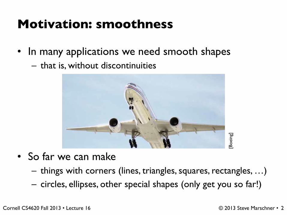
Motivation: smoothness
• In many applications we need smooth shapes– that is, without discontinuities
• So far we can make– things with corners (lines, triangles, squares, rectangles, …)– circles, ellipses, other special shapes (only get you so far!)
[Boe
ing]
2

© 2013 Steve Marschner • Cornell CS4620 Fall 2013 • Lecture 16
Classical approach
• Pencil-and-paper draftsmen also needed smooth curves• Origin of “spline:” strip of flexible metal
– held in place by pegs or weights to constrain shape– traced to produce smooth contour
3
© 2013 Steve Marschner • Cornell CS4620 Fall 2013 • Lecture 16
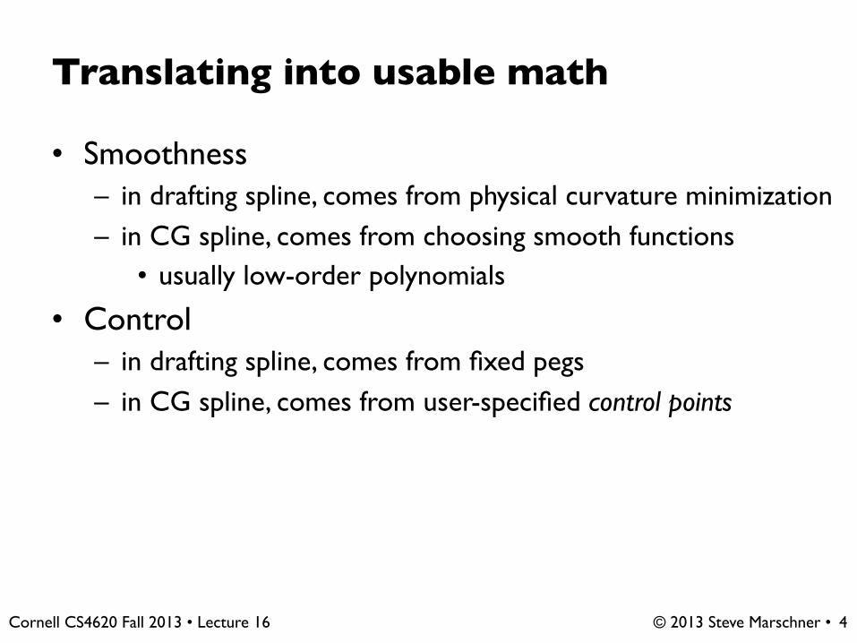
Translating into usable math
• Smoothness– in drafting spline, comes from physical curvature minimization– in CG spline, comes from choosing smooth functions
• usually low-order polynomials
• Control– in drafting spline, comes from fixed pegs– in CG spline, comes from user-specified control points
4

© 2013 Steve Marschner • Cornell CS4620 Fall 2013 • Lecture 16
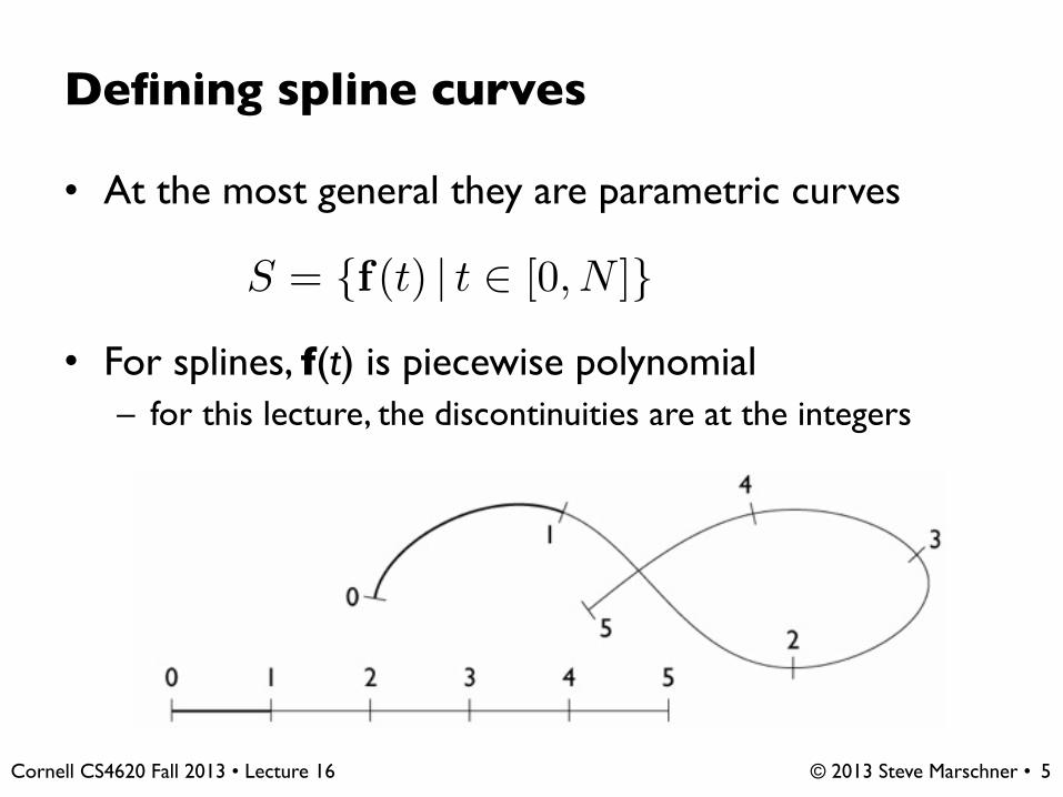
Defining spline curves
• At the most general they are parametric curves
• For splines, f(t) is piecewise polynomial– for this lecture, the discontinuities are at the integers
5
S = {f(t) | t 2 [0, N ]}
© 2013 Steve Marschner • Cornell CS4620 Fall 2013 • Lecture 16
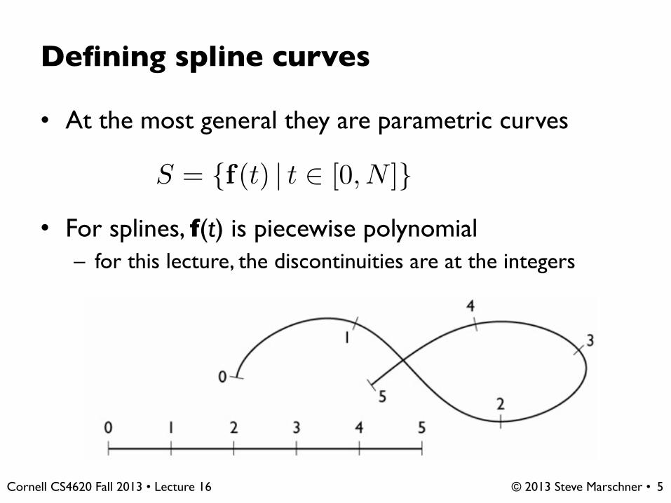
Defining spline curves
• At the most general they are parametric curves
• For splines, f(t) is piecewise polynomial– for this lecture, the discontinuities are at the integers
5
S = {f(t) | t 2 [0, N ]}

© 2013 Steve Marschner • Cornell CS4620 Fall 2013 • Lecture 16
Defining spline curves
• At the most general they are parametric curves
• For splines, f(t) is piecewise polynomial– for this lecture, the discontinuities are at the integers
5
S = {f(t) | t 2 [0, N ]}
© 2013 Steve Marschner • Cornell CS4620 Fall 2013 • Lecture 16
Defining spline curves
• At the most general they are parametric curves
• For splines, f(t) is piecewise polynomial– for this lecture, the discontinuities are at the integers
5
S = {f(t) | t 2 [0, N ]}
© 2013 Steve Marschner • Cornell CS4620 Fall 2013 • Lecture 16
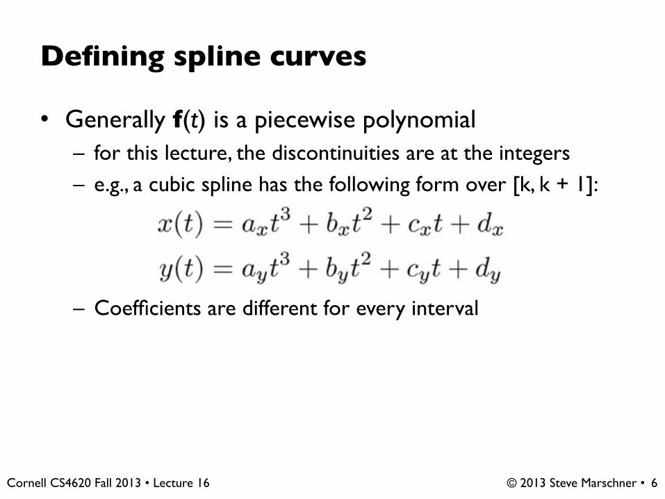
Defining spline curves
• Generally f(t) is a piecewise polynomial– for this lecture, the discontinuities are at the integers– e.g., a cubic spline has the following form over [k, k + 1]:
– Coefficients are different for every interval
6
© 2013 Steve Marschner • Cornell CS4620 Fall 2013 • Lecture 16
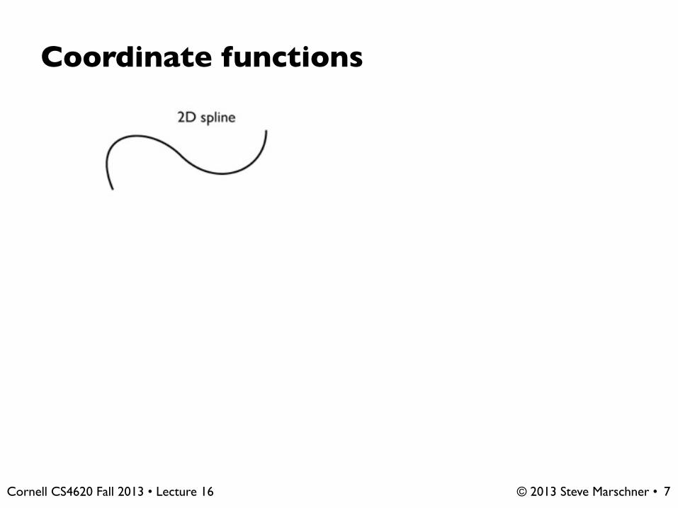
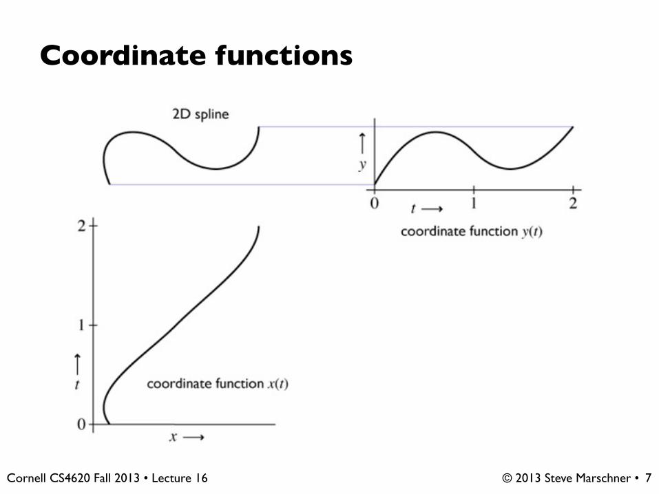
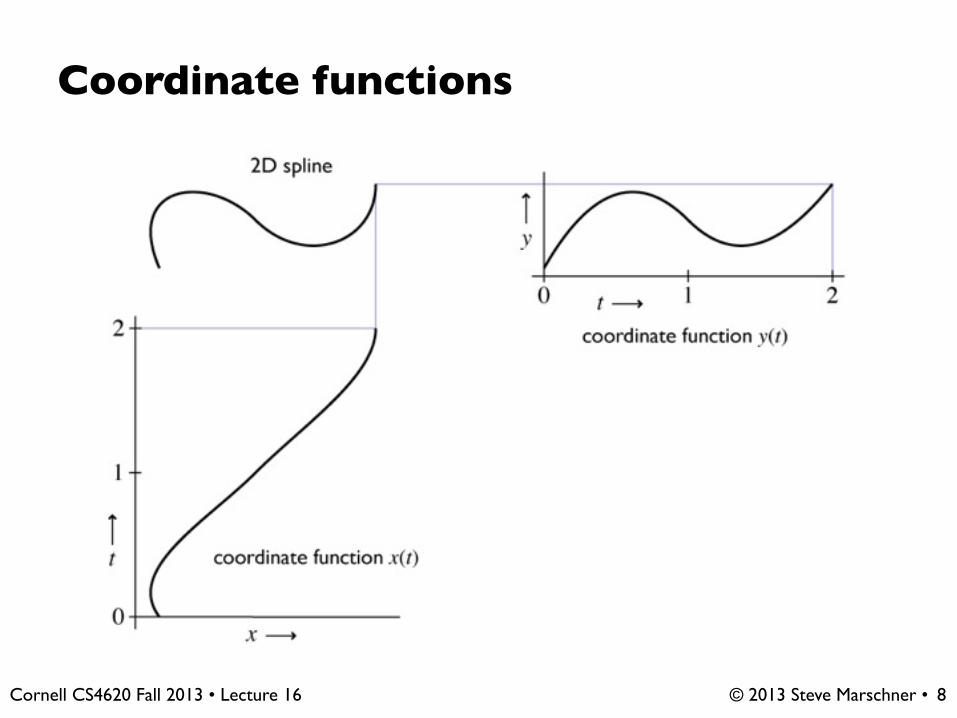
Coordinate functions
7

© 2013 Steve Marschner • Cornell CS4620 Fall 2013 • Lecture 16
Coordinate functions
7
© 2013 Steve Marschner • Cornell CS4620 Fall 2013 • Lecture 16
Coordinate functions
7

© 2013 Steve Marschner • Cornell CS4620 Fall 2013 • Lecture 16
Coordinate functions
7

© 2013 Steve Marschner • Cornell CS4620 Fall 2013 • Lecture 16
Coordinate functions
8

© 2013 Steve Marschner • Cornell CS4620 Fall 2013 • Lecture 16
Coordinate functions
8

© 2013 Steve Marschner • Cornell CS4620 Fall 2013 • Lecture 16
Coordinate functions
8

© 2013 Steve Marschner • Cornell CS4620 Fall 2013 • Lecture 16
Coordinate functions
8
© 2013 Steve Marschner • Cornell CS4620 Fall 2013 • Lecture 16
Coordinate functions
8

© 2013 Steve Marschner • Cornell CS4620 Fall 2013 • Lecture 16
Control of spline curves
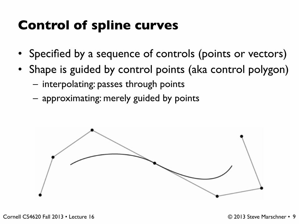
• Specified by a sequence of controls (points or vectors)• Shape is guided by control points (aka control polygon)
– interpolating: passes through points– approximating: merely guided by points
9

© 2013 Steve Marschner • Cornell CS4620 Fall 2013 • Lecture 16
Control of spline curves
• Specified by a sequence of controls (points or vectors)• Shape is guided by control points (aka control polygon)
– interpolating: passes through points– approximating: merely guided by points
9
© 2013 Steve Marschner • Cornell CS4620 Fall 2013 • Lecture 16
Control of spline curves
• Specified by a sequence of controls (points or vectors)• Shape is guided by control points (aka control polygon)
– interpolating: passes through points– approximating: merely guided by points
9

© 2013 Steve Marschner • Cornell CS4620 Fall 2013 • Lecture 16
Control of spline curves
• Specified by a sequence of controls (points or vectors)• Shape is guided by control points (aka control polygon)
– interpolating: passes through points– approximating: merely guided by points
9
© 2013 Steve Marschner • Cornell CS4620 Fall 2013 • Lecture 16
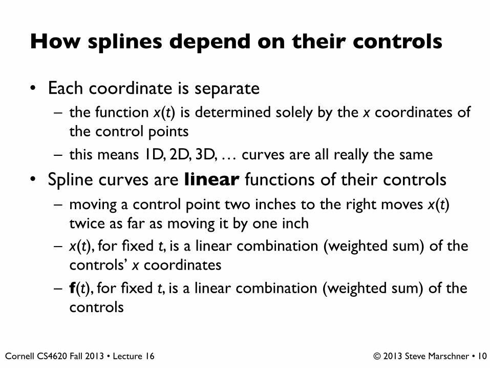
How splines depend on their controls
• Each coordinate is separate– the function x(t) is determined solely by the x coordinates of
the control points– this means 1D, 2D, 3D, … curves are all really the same
• Spline curves are linear functions of their controls– moving a control point two inches to the right moves x(t)
twice as far as moving it by one inch– x(t), for fixed t, is a linear combination (weighted sum) of the
controls’ x coordinates– f(t), for fixed t, is a linear combination (weighted sum) of the
controls
10

© 2013 Steve Marschner • Cornell CS4620 Fall 2013 • Lecture 16
Plan
1. Spline segments– how to define a polynomial on [0,1]– …that has the properties you want– …and is easy to control
2. Spline curves– how to chain together lots of segments– …so that the whole curve has the properties you want– …and is easy to control
3. Refinement and evaluation– how to add detail to splines– how to approximate them with line segments
11

© 2013 Steve Marschner • Cornell CS4620 Fall 2013 • Lecture 16
Spline Segments
12

© 2013 Steve Marschner • Cornell CS4620 Fall 2013 • Lecture 16
Trivial example: piecewise linear
• This spline is just a polygon– control points are the vertices
• But we can derive it anyway as an illustration• Each interval will be a linear function
– x(t) = at + b– constraints are values at endpoints
– b = x0 ; a = x1 – x0
– this is linear interpolation
13
© 2013 Steve Marschner • Cornell CS4620 Fall 2013 • Lecture 16
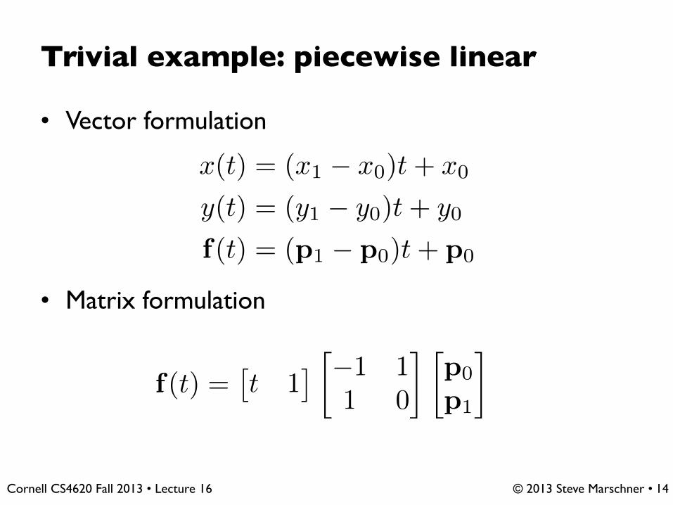
Trivial example: piecewise linear
• Vector formulation
• Matrix formulation
14
f(t) =⇥t 1
⇤ �1 11 0
� p0
p1
�
x(t) = (x1 � x0)t+ x0
y(t) = (y1 � y0)t+ y0
f(t) = (p1 � p0)t+ p0
© 2013 Steve Marschner • Cornell CS4620 Fall 2013 • Lecture 16
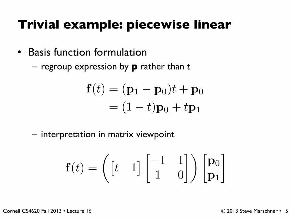
Trivial example: piecewise linear
• Basis function formulation– regroup expression by p rather than t
– interpretation in matrix viewpoint
15
f(t) = (p1 � p0)t+ p0
= (1� t)p0 + tp1
f(t) =
✓⇥t 1
⇤ �1 11 0
�◆p0
p1
�
© 2013 Steve Marschner • Cornell CS4620 Fall 2013 • Lecture 16
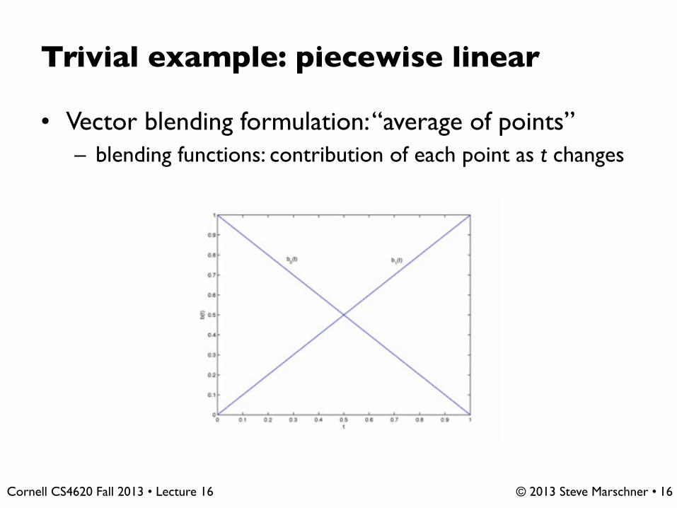
Trivial example: piecewise linear
• Vector blending formulation: “average of points”– blending functions: contribution of each point as t changes
16
© 2013 Steve Marschner • Cornell CS4620 Fall 2013 • Lecture 16
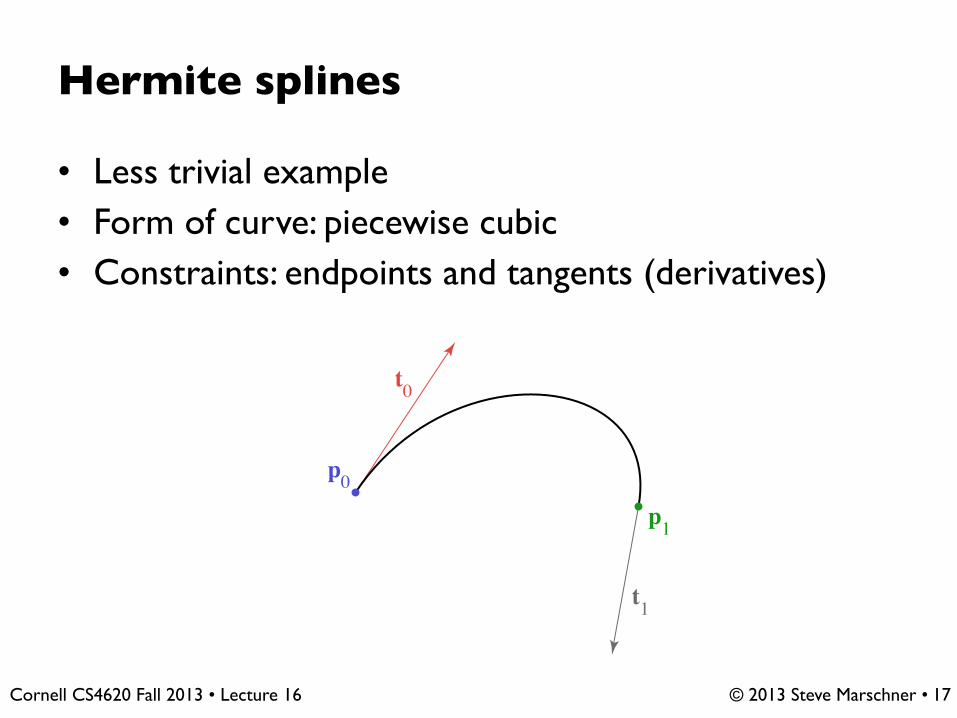
Hermite splines
• Less trivial example• Form of curve: piecewise cubic• Constraints: endpoints and tangents (derivatives)
17
t0
p1
p0
t1

© 2013 Steve Marschner • Cornell CS4620 Fall 2013 • Lecture 16
Hermite splines
• Solve constraints to find coefficients
18
x(t) = at
3 + bt
2 + ct+ d
x
0(t) = 3at2 + 2bt+ c
x(0) = x0 = d
x(1) = x1 = a+ b+ c+ d
x
0(0) = x
00 = c
x
0(1) = x
01 = 3a+ 2b+ c
d = x0
c = x
00
a = 2x0 � 2x1 + x
00 + x
01
b = �3x0 + 3x1 � 2x00 � x
01

© 2013 Steve Marschner • Cornell CS4620 Fall 2013 • Lecture 16
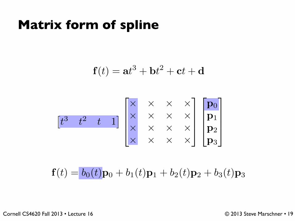
Matrix form of spline
19
⇥t3 t2 t 1
⇤
2
664
⇥ ⇥ ⇥ ⇥⇥ ⇥ ⇥ ⇥⇥ ⇥ ⇥ ⇥⇥ ⇥ ⇥ ⇥
3
775
2
664
p0
p1
p2
p3
3
775
f(t) = b0(t)p0 + b1(t)p1 + b2(t)p2 + b3(t)p3
f(t) = at3 + bt2 + ct+ d

© 2013 Steve Marschner • Cornell CS4620 Fall 2013 • Lecture 16
Matrix form of spline
19
⇥t3 t2 t 1
⇤
2
664
⇥ ⇥ ⇥ ⇥⇥ ⇥ ⇥ ⇥⇥ ⇥ ⇥ ⇥⇥ ⇥ ⇥ ⇥
3
775
2
664
p0
p1
p2
p3
3
775
f(t) = b0(t)p0 + b1(t)p1 + b2(t)p2 + b3(t)p3
f(t) = at3 + bt2 + ct+ d
© 2013 Steve Marschner • Cornell CS4620 Fall 2013 • Lecture 16
Matrix form of spline
19
⇥t3 t2 t 1
⇤
2
664
⇥ ⇥ ⇥ ⇥⇥ ⇥ ⇥ ⇥⇥ ⇥ ⇥ ⇥⇥ ⇥ ⇥ ⇥
3
775
2
664
p0
p1
p2
p3
3
775
f(t) = b0(t)p0 + b1(t)p1 + b2(t)p2 + b3(t)p3
f(t) = at3 + bt2 + ct+ d

© 2013 Steve Marschner • Cornell CS4620 Fall 2013 • Lecture 16
Hermite splines
• Matrix form is much simpler
– coefficients = rows– basis functions = columns
• note p columns sum to [0 0 0 1]T
20
f(t) =⇥t3 t2 t 1
⇤
2
664
2 �2 1 1�3 3 �2 �10 0 1 01 0 0 0
3
775
2
664
p0
p1
t0t1
3
775

© 2013 Steve Marschner • Cornell CS4620 Fall 2013 • Lecture 16
Hermite splines
• Hermite blending functions
21

© 2013 Steve Marschner • Cornell CS4620 Fall 2013 • Lecture 16
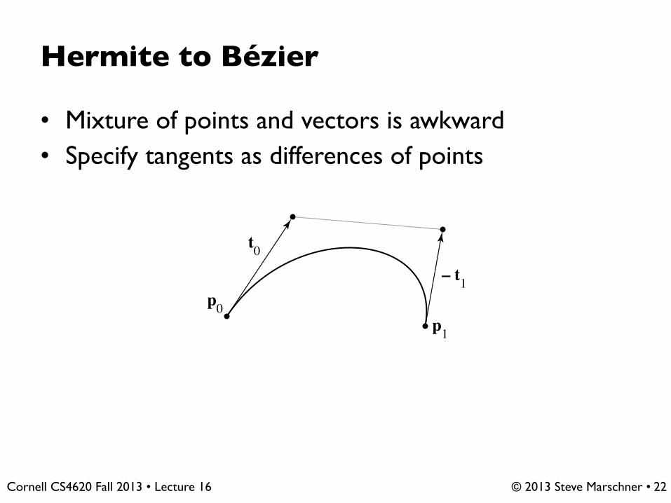
Hermite to Bézier
• Mixture of points and vectors is awkward• Specify tangents as differences of points
22
p0
t0
p1
t1

© 2013 Steve Marschner • Cornell CS4620 Fall 2013 • Lecture 16
Hermite to Bézier
• Mixture of points and vectors is awkward• Specify tangents as differences of points
22
p0
t0
p1
– t1
© 2013 Steve Marschner • Cornell CS4620 Fall 2013 • Lecture 16
Hermite to Bézier
• Mixture of points and vectors is awkward• Specify tangents as differences of points
22
p0
t0
p1
– t1

© 2013 Steve Marschner • Cornell CS4620 Fall 2013 • Lecture 16
Hermite to Bézier
• Mixture of points and vectors is awkward• Specify tangents as differences of points
– note derivative is defined as 3 times offset• reason is illustrated by linear case
22
p0
t0
p1
– t1
q0
q1 q2
q3
I’m calling these points q just for this slide and the next one.
© 2013 Steve Marschner • Cornell CS4620 Fall 2013 • Lecture 16
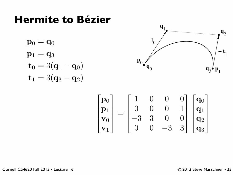
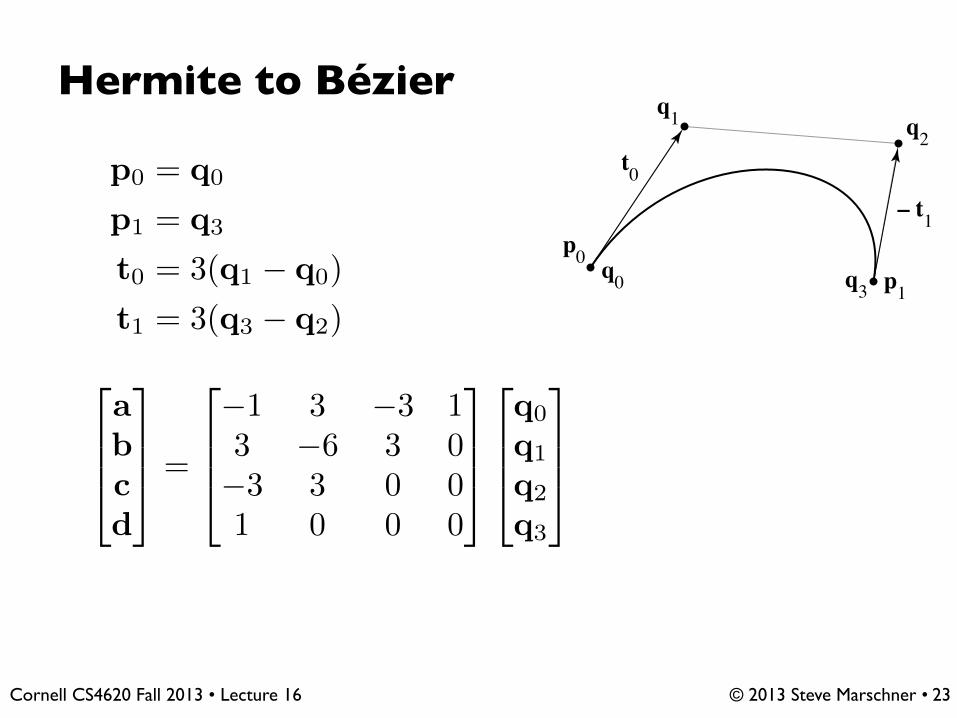
Hermite to Bézier
23
p0
t0
p1
– t1
q0
q1 q2
q3
p0 = q0
p1 = q3
t0 = 3(q1 � q0)
t1 = 3(q3 � q2)
2
664
p0
p1
v0
v1
3
775 =
2
664
1 0 0 00 0 0 1�3 3 0 00 0 �3 3
3
775
2
664
q0
q1
q2
q3
3
775

© 2013 Steve Marschner • Cornell CS4620 Fall 2013 • Lecture 16
Hermite to Bézier
23
p0
t0
p1
– t1
q0
q1 q2
q3
p0 = q0
p1 = q3
t0 = 3(q1 � q0)
t1 = 3(q3 � q2)
2
664
abcd
3
775 =
2
664
2 �2 1 1�3 3 �2 �10 0 1 01 0 0 0
3
775
2
664
1 0 0 00 0 0 1�3 3 0 00 0 �3 3
3
775
2
664
q0
q1
q2
q3
3
775
© 2013 Steve Marschner • Cornell CS4620 Fall 2013 • Lecture 16
Hermite to Bézier
23
p0
t0
p1
– t1
q0
q1 q2
q3
p0 = q0
p1 = q3
t0 = 3(q1 � q0)
t1 = 3(q3 � q2)
2
664
abcd
3
775 =
2
664
�1 3 �3 13 �6 3 0�3 3 0 01 0 0 0
3
775
2
664
q0
q1
q2
q3
3
775

© 2013 Steve Marschner • Cornell CS4620 Fall 2013 • Lecture 16
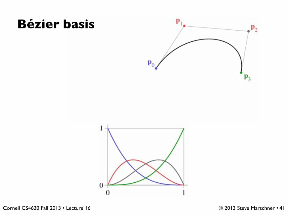
Bézier matrix
– note that these are the Bernstein polynomials
and that defines Bézier curves for any degree
24
f(t) =⇥t3 t2 t 1
⇤
2
664
�1 3 �3 13 �6 3 0�3 3 0 01 0 0 0
3
775
2
664
p0
p1
p2
p3
3
775
bn,k(t) =
✓n
k
◆tk(1� t)n�k

© 2013 Steve Marschner • Cornell CS4620 Fall 2013 • Lecture 16
Bézier basis
25

© 2013 Steve Marschner • Cornell CS4620 Fall 2013 • Lecture 16
Another way to Bézier segments
• A really boring spline segment: f(t) = p0– it only has one control point– the curve stays at that point for the whole time
• Only good for building a piecewise constant spline– a.k.a. a set of points
26
p0

© 2013 Steve Marschner • Cornell CS4620 Fall 2013 • Lecture 16
Another way to Bézier segments
• A piecewise linear spline segment– two control points per segment– blend them with weights α and β = 1 – α
• Good for building a piecewise linear spline– a.k.a. a polygon or polyline
27
Ơ
ơ
p0
Ơp0 + ơp1
p1
These labels show the weights, not the distances.

© 2013 Steve Marschner • Cornell CS4620 Fall 2013 • Lecture 16
Another way to Bézier segments
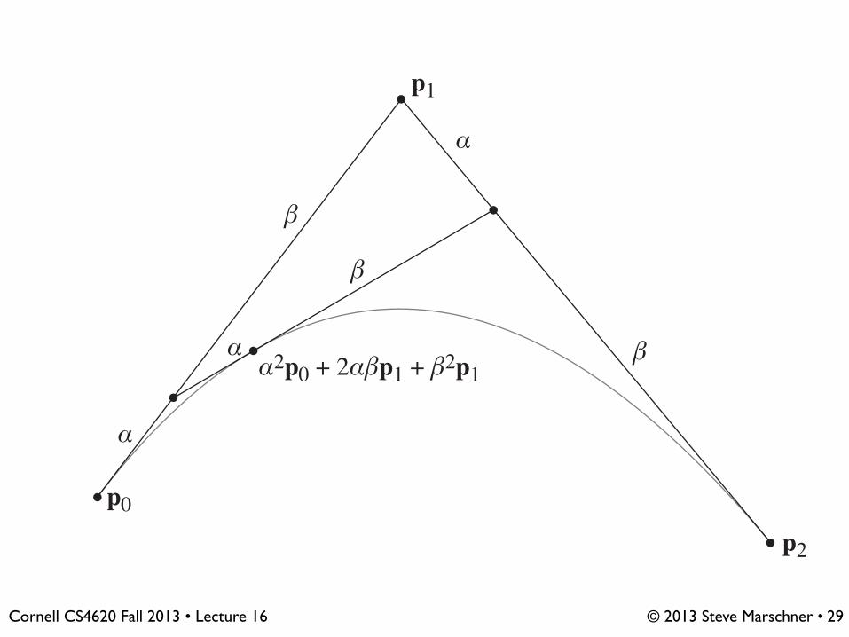
• A linear blend of two piecewise linear segments– three control points now– interpolate on both segments using α and β– blend the results with the same weights
• makes a quadratic spline segment– finally, a curve!
28
p1,0 = ↵p0 + �p1
p1,1 = ↵p1 + �p2
p2,0 = ↵p1,0 + �p1,1
= ↵↵p0 + ↵�p1 + �↵p1 + ��p2
= ↵2p0 + 2↵�p1 + �2p2
© 2013 Steve Marschner • Cornell CS4620 Fall 2013 • Lecture 16 29
Ơ
Ơ
Ơ
ơ
ơ
ơ
Ơ2p0 + 2Ơơp1 + ơ2p1
p0
p2
p1

© 2013 Steve Marschner • Cornell CS4620 Fall 2013 • Lecture 16
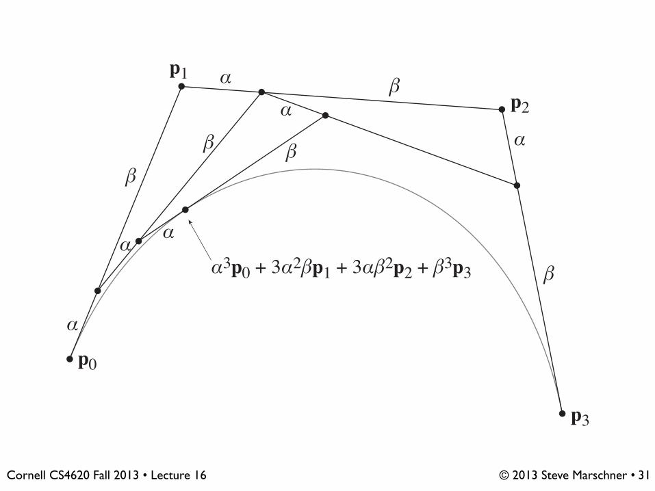
Another way to Bézier segments
• Cubic segment: blend of two quadratic segments– four control points now (overlapping sets of 3)– interpolate on each quadratic using α and β– blend the results with the same weights
• makes a cubic spline segment– this is the familiar one for graphics—but you can keep going
30
p3,0 =↵p2,0 + �p2,1
=↵↵↵p0 + ↵↵�p1 + ↵�↵p1 + ↵��p2
�↵↵p1 + �↵�p2 + ��↵p2 + ���p3
=↵3p0 + 3↵2�p1 + 3↵�2p2 + �3p3
© 2013 Steve Marschner • Cornell CS4620 Fall 2013 • Lecture 16 31
Ơ
Ơ Ơ
ƠƠ
Ơ
ơ
ơ
ơ
ơơ
Ơ3p0 + 3Ơ2ơp1 + 3Ơơ2p2 + ơ3p3
p0
p2
p3
p1

© 2013 Steve Marschner • Cornell CS4620 Fall 2013 • Lecture 16
de Casteljau’s algorithm
• A recurrence for computing points on Bézier spline segments:
• Cool additional feature:also subdivides the segment into twoshorter ones
[FvD
FH]
32
p0,i = pi
pn,i = ↵pn�1,i + �pn�1,i+1
© 2013 Steve Marschner • Cornell CS4620 Fall 2013 • Lecture 16
Cubic Bézier splines
• Very widely used type, especially in 2D– e.g. it is a primitive in PostScript/PDF
• Can represent smooth curves with corners• Nice de Casteljau recurrence for evaluation• Can easily add points at any position• Illustrator demo
33

© 2013 Steve Marschner • Cornell CS4620 Fall 2013 • Lecture 16
Spline Curves
34

© 2013 Steve Marschner • Cornell CS4620 Fall 2013 • Lecture 16
Chaining spline segments
• Can only do so much with a single polynomial• Can use these functions as segments of a longer curve
– curve from t = 0 to t = 1 defined by first segment– curve from t = 1 to t = 2 defined by second segment
• To avoid discontinuity, match derivatives at junctions– this produces a C1 curve
35
f(t) = fi(t� i) for i t i+ 1
© 2013 Steve Marschner • Cornell CS4620 Fall 2013 • Lecture 16
Trivial example: piecewise linear
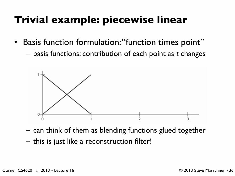
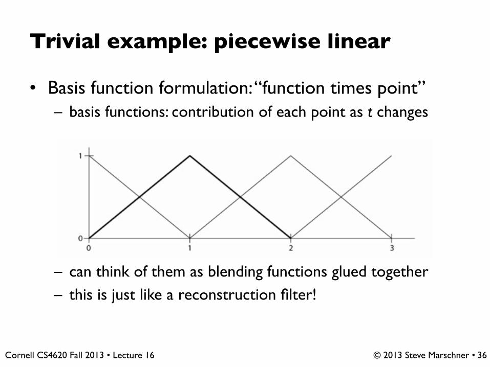
• Basis function formulation: “function times point”– basis functions: contribution of each point as t changes
– can think of them as blending functions glued together– this is just like a reconstruction filter!
36
© 2013 Steve Marschner • Cornell CS4620 Fall 2013 • Lecture 16
Trivial example: piecewise linear
• Basis function formulation: “function times point”– basis functions: contribution of each point as t changes
– can think of them as blending functions glued together– this is just like a reconstruction filter!
36

© 2013 Steve Marschner • Cornell CS4620 Fall 2013 • Lecture 16
Splines as reconstruction
37

© 2013 Steve Marschner • Cornell CS4620 Fall 2013 • Lecture 16
Splines as reconstruction
37
© 2013 Steve Marschner • Cornell CS4620 Fall 2013 • Lecture 16
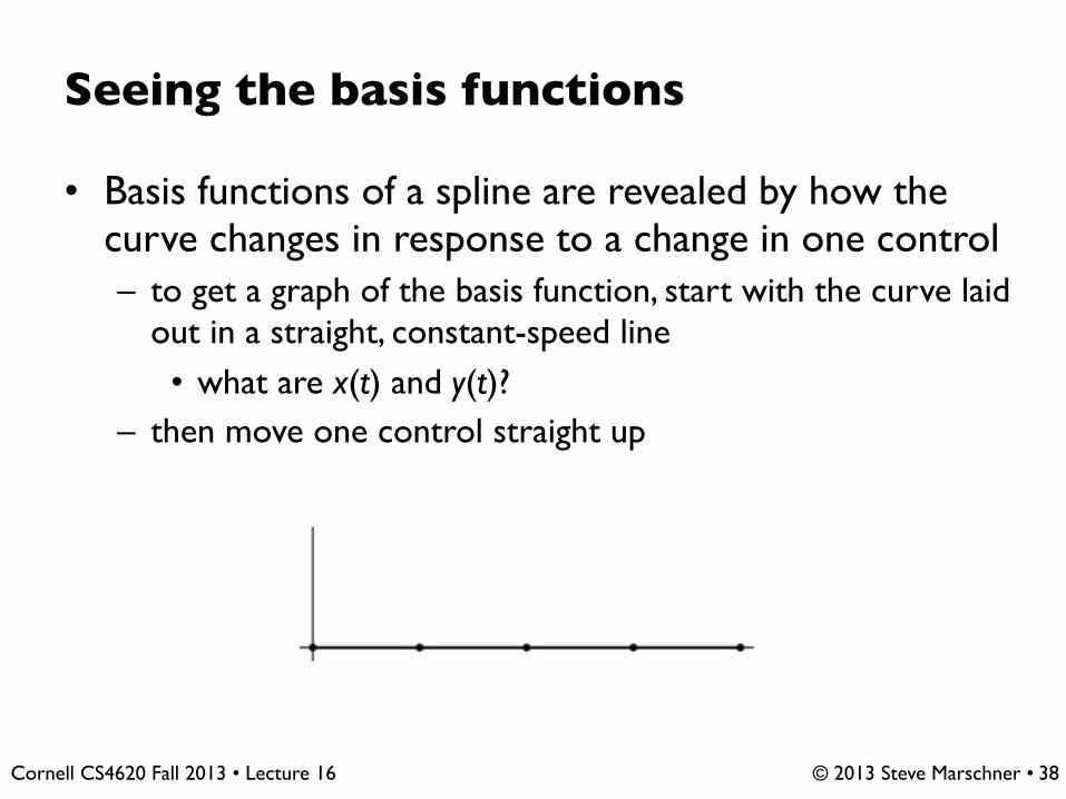
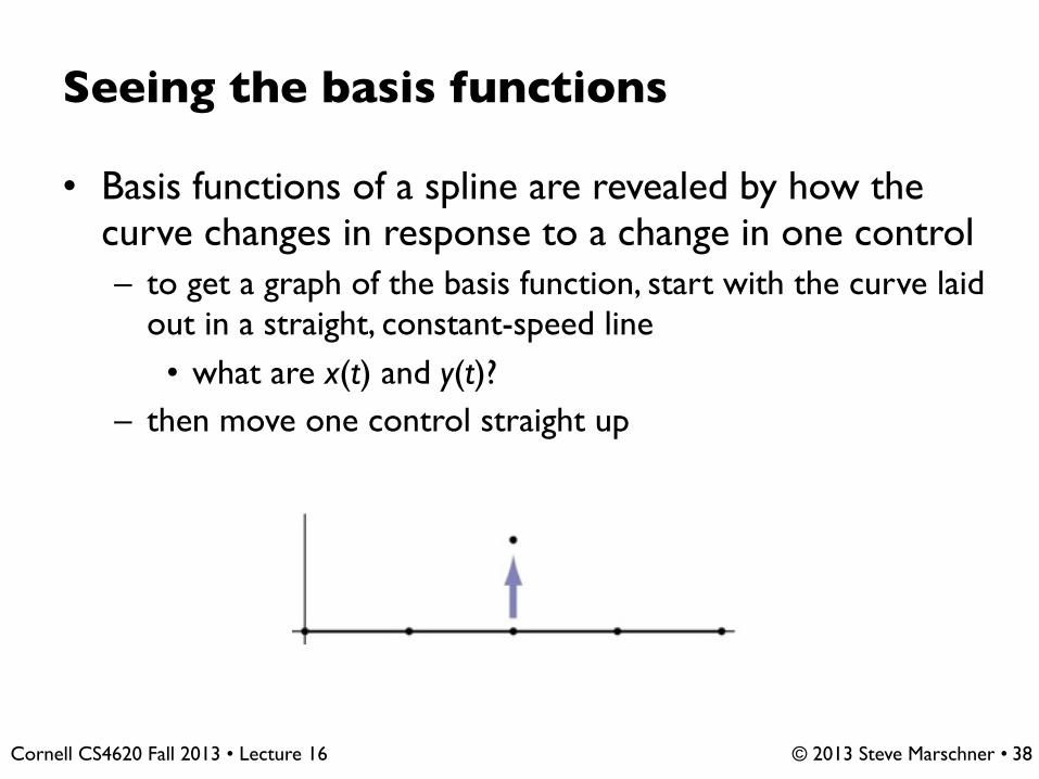
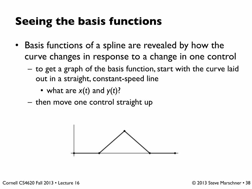
Seeing the basis functions
• Basis functions of a spline are revealed by how the curve changes in response to a change in one control– to get a graph of the basis function, start with the curve laid
out in a straight, constant-speed line• what are x(t) and y(t)?
– then move one control straight up
38
© 2013 Steve Marschner • Cornell CS4620 Fall 2013 • Lecture 16
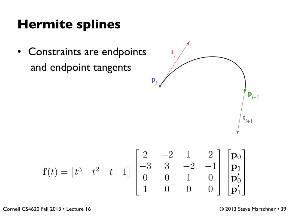
Hermite splines
• Constraints are endpoints
and endpoint tangents
39
f(t) =⇥t3 t2 t 1
⇤
2
664
2 �2 1 2�3 3 �2 �10 0 1 01 0 0 0
3
775
2
664
p0
p1
p00
p01
3
775
ti
pi+1
pi
ti+1

© 2013 Steve Marschner • Cornell CS4620 Fall 2013 • Lecture 16
Hermite basis
40

© 2013 Steve Marschner • Cornell CS4620 Fall 2013 • Lecture 16
Hermite basis
40
00 1
1p1
t0
p0
t1
ti
pi+1
pi
ti+1

© 2013 Steve Marschner • Cornell CS4620 Fall 2013 • Lecture 16
Hermite basis
40
0
1
i i + 1i – 1 i + 2
pi+1
ti
pi
ti+1
ti
pi+1
pi
ti+1
pi–1
ti–1 ti+2 pi+2
© 2013 Steve Marschner • Cornell CS4620 Fall 2013 • Lecture 16
Bézier basis
41
© 2013 Steve Marschner • Cornell CS4620 Fall 2013 • Lecture 16
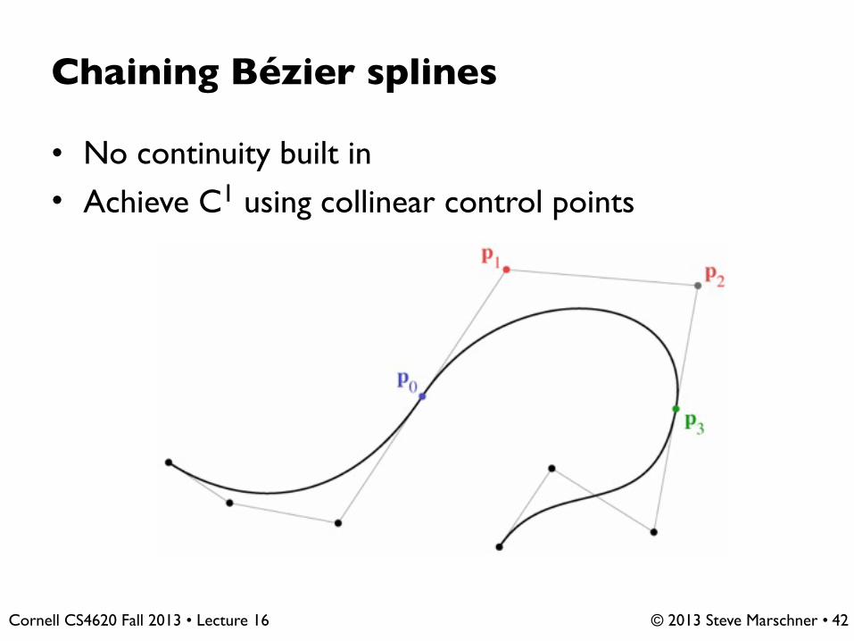
Chaining Bézier splines
• No continuity built in• Achieve C1 using collinear control points
42
© 2013 Steve Marschner • Cornell CS4620 Fall 2013 • Lecture 16
Chaining Bézier splines
• No continuity built in• Achieve C1 using collinear control points
42
© 2013 Steve Marschner • Cornell CS4620 Fall 2013 • Lecture 16
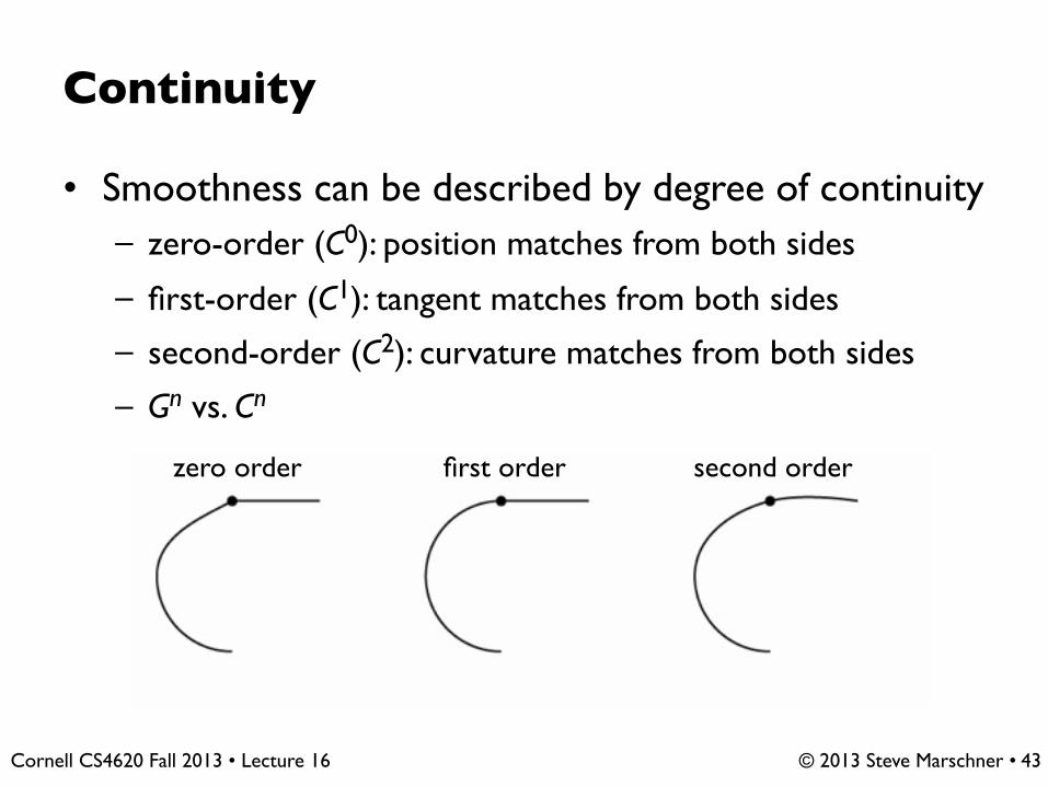
Continuity
• Smoothness can be described by degree of continuity– zero-order (C0): position matches from both sides
– first-order (C1): tangent matches from both sides
– second-order (C2): curvature matches from both sides
– Gn vs. Cn
zero order first order second order
43
© 2013 Steve Marschner • Cornell CS4620 Fall 2013 • Lecture 16
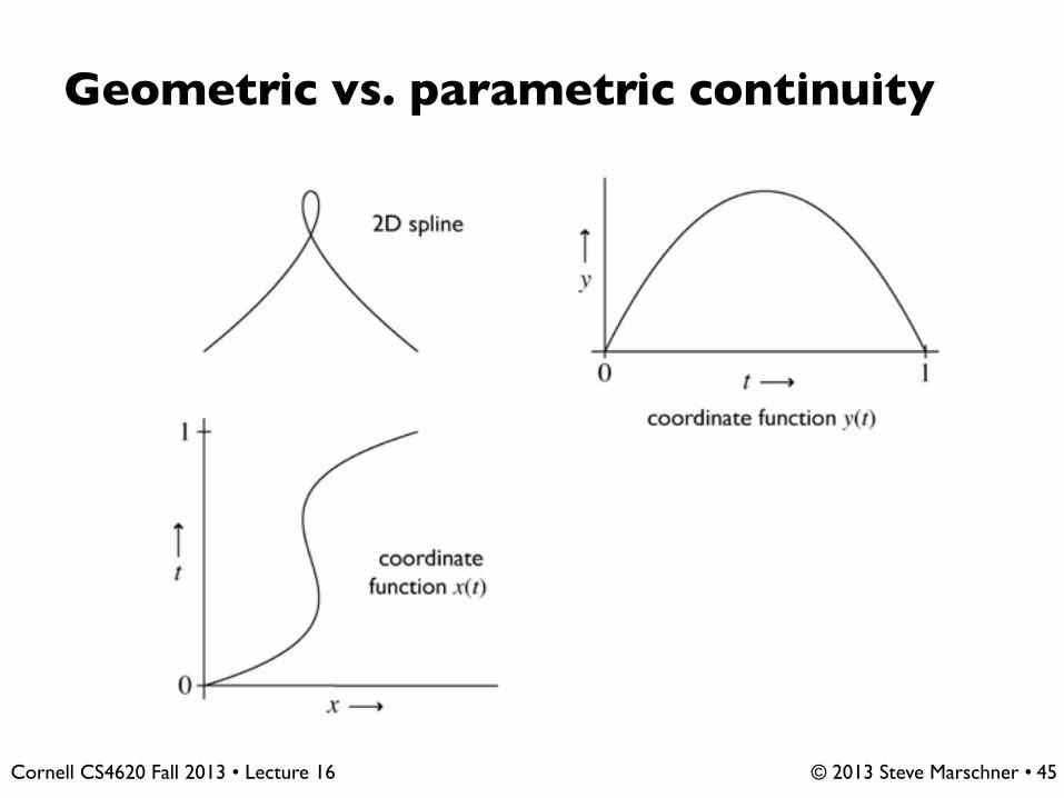
Continuity
• Parametric continuity (C) of spline is continuity of coordinate functions
• Geometric continuity (G) is continuity of the curve itself
• Neither form of continuity is guaranteed by the other– Can be C1 but not G1 when p(t) comes to a halt (next slide)
– Can be G1 but not C1 when the tangent vector changes length abruptly
44

© 2013 Steve Marschner • Cornell CS4620 Fall 2013 • Lecture 16
Geometric vs. parametric continuity
45

© 2013 Steve Marschner • Cornell CS4620 Fall 2013 • Lecture 16
Geometric vs. parametric continuity
45
© 2013 Steve Marschner • Cornell CS4620 Fall 2013 • Lecture 16
Geometric vs. parametric continuity
45
© 2013 Steve Marschner • Cornell CS4620 Fall 2013 • Lecture 16
Control
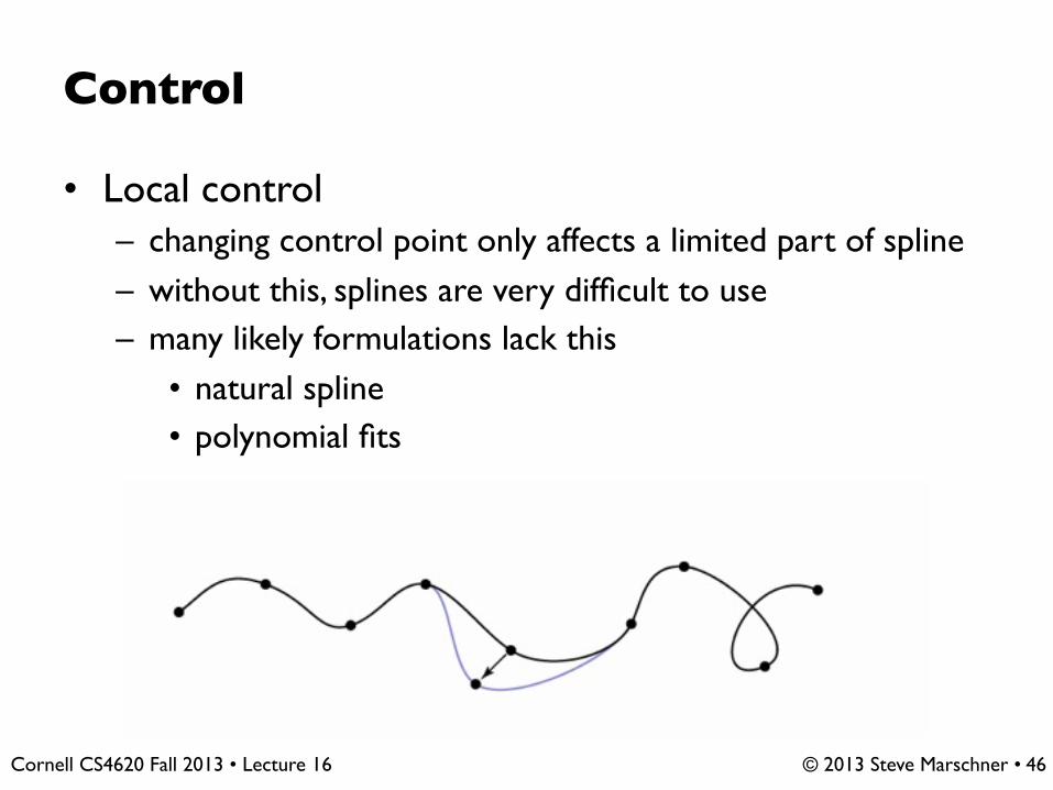
• Local control– changing control point only affects a limited part of spline– without this, splines are very difficult to use– many likely formulations lack this
• natural spline• polynomial fits
46
© 2013 Steve Marschner • Cornell CS4620 Fall 2013 • Lecture 16
Control
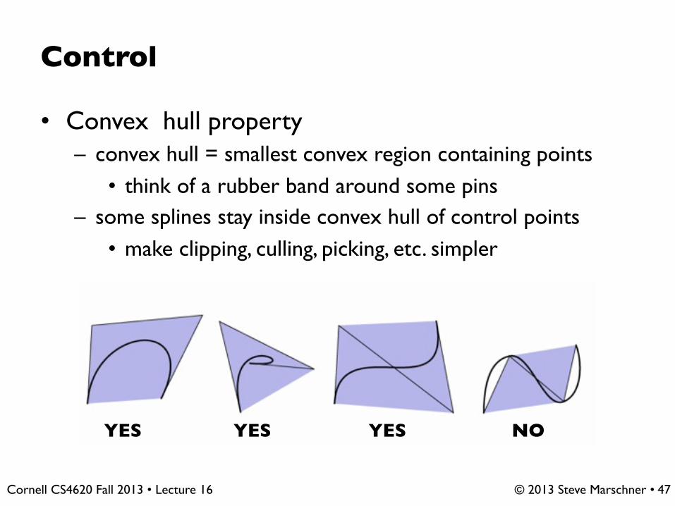
• Convex hull property– convex hull = smallest convex region containing points
• think of a rubber band around some pins– some splines stay inside convex hull of control points
• make clipping, culling, picking, etc. simpler
YES YES YES NO
47

© 2013 Steve Marschner • Cornell CS4620 Fall 2013 • Lecture 16
Convex hull
• If basis functions are all positive, the spline has the convex hull property– we’re still requiring them to sum to 1
– if any basis function is ever negative, no convex hull prop.• proof: take the other three points at the same place
48
© 2013 Steve Marschner • Cornell CS4620 Fall 2013 • Lecture 16
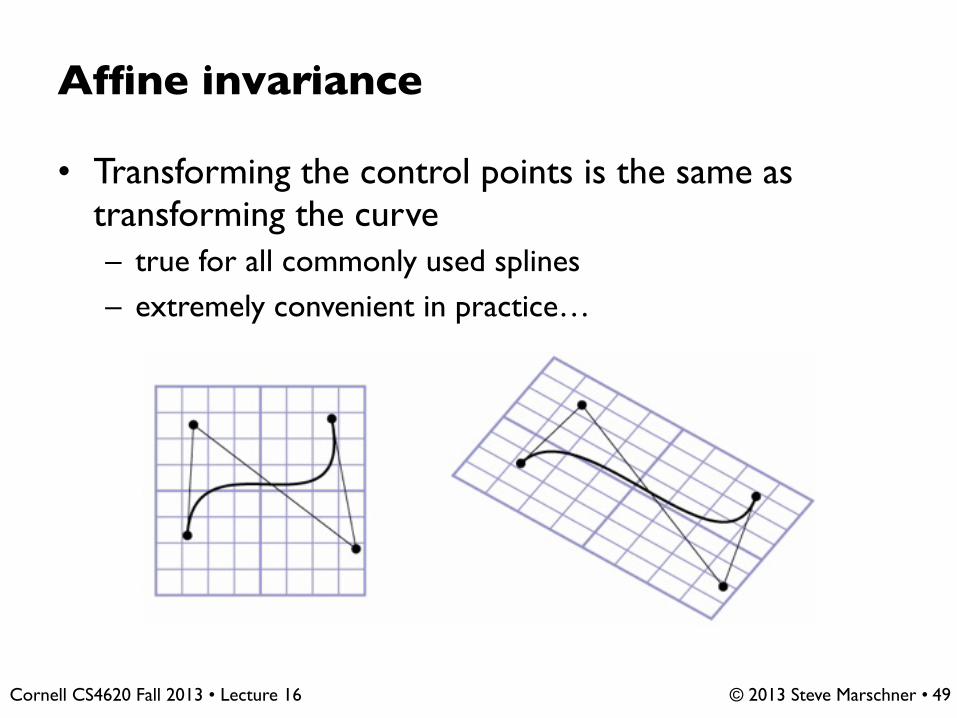
Affine invariance
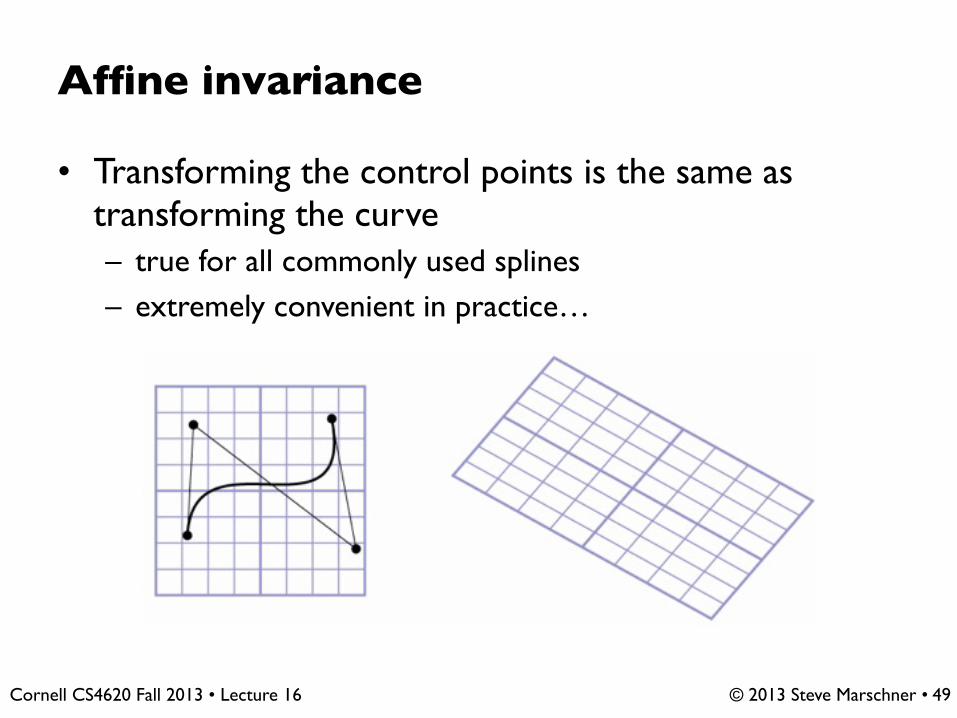
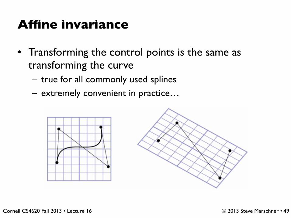
• Transforming the control points is the same as transforming the curve– true for all commonly used splines– extremely convenient in practice…
49
© 2013 Steve Marschner • Cornell CS4620 Fall 2013 • Lecture 16
Affine invariance
• Transforming the control points is the same as transforming the curve– true for all commonly used splines– extremely convenient in practice…
49
© 2013 Steve Marschner • Cornell CS4620 Fall 2013 • Lecture 16
Affine invariance
• Transforming the control points is the same as transforming the curve– true for all commonly used splines– extremely convenient in practice…
49
© 2013 Steve Marschner • Cornell CS4620 Fall 2013 • Lecture 16
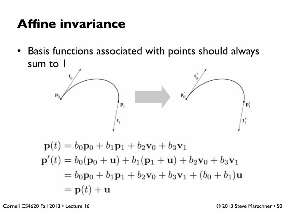
Affine invariance
• Basis functions associated with points should always sum to 1
50
© 2013 Steve Marschner • Cornell CS4620 Fall 2013 • Lecture 16
Chaining spline segments
• Hermite curves are convenient because they can be made long easily
• Bézier curves are convenient because their controls are all points– but it is fussy to maintain continuity constraints– and they interpolate every 3rd point, which is a little odd
• We derived Bézier from Hermite by defining tangents from control points– a similar construction leads to the interpolating Catmull-Rom
spline
51
© 2013 Steve Marschner • Cornell CS4620 Fall 2013 • Lecture 16
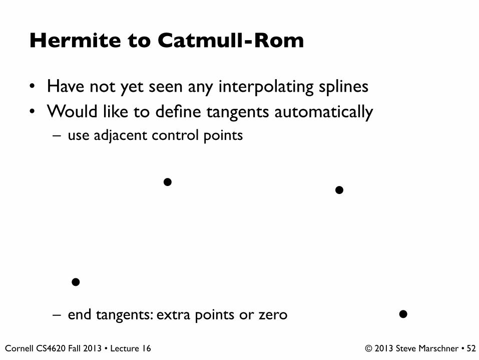
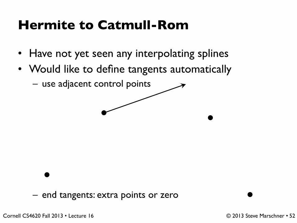
• Have not yet seen any interpolating splines• Would like to define tangents automatically
– use adjacent control points
– end tangents: extra points or zero
Hermite to Catmull-Rom
52

© 2013 Steve Marschner • Cornell CS4620 Fall 2013 • Lecture 16
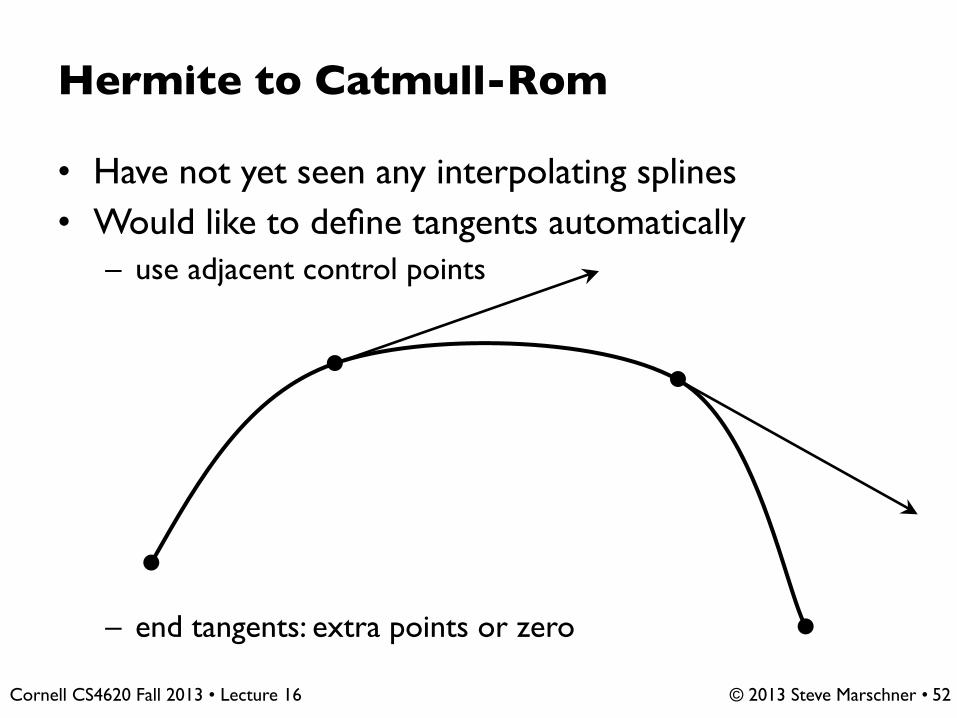
• Have not yet seen any interpolating splines• Would like to define tangents automatically
– use adjacent control points
– end tangents: extra points or zero
Hermite to Catmull-Rom
52
© 2013 Steve Marschner • Cornell CS4620 Fall 2013 • Lecture 16
• Have not yet seen any interpolating splines• Would like to define tangents automatically
– use adjacent control points
– end tangents: extra points or zero
Hermite to Catmull-Rom
52

© 2013 Steve Marschner • Cornell CS4620 Fall 2013 • Lecture 16
• Have not yet seen any interpolating splines• Would like to define tangents automatically
– use adjacent control points
– end tangents: extra points or zero
Hermite to Catmull-Rom
52

© 2013 Steve Marschner • Cornell CS4620 Fall 2013 • Lecture 16
• Have not yet seen any interpolating splines• Would like to define tangents automatically
– use adjacent control points
– end tangents: extra points or zero
Hermite to Catmull-Rom
52
© 2013 Steve Marschner • Cornell CS4620 Fall 2013 • Lecture 16
• Have not yet seen any interpolating splines• Would like to define tangents automatically
– use adjacent control points
– end tangents: extra points or zero
Hermite to Catmull-Rom
52
© 2013 Steve Marschner • Cornell CS4620 Fall 2013 • Lecture 16
Hermite to Catmull-Rom
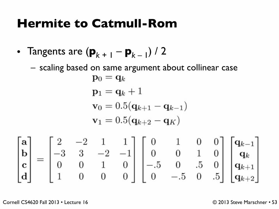
• Tangents are (pk + 1 – pk – 1) / 2
– scaling based on same argument about collinear case
53

© 2013 Steve Marschner • Cornell CS4620 Fall 2013 • Lecture 16
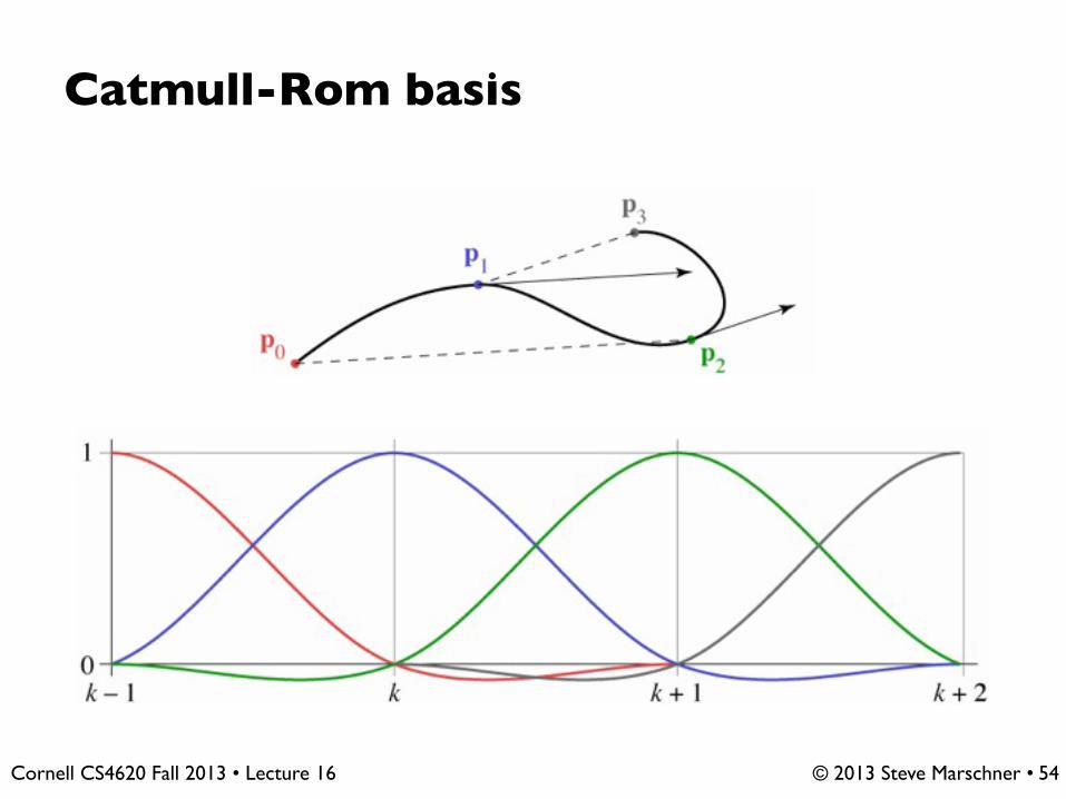
Catmull-Rom basis
54
© 2013 Steve Marschner • Cornell CS4620 Fall 2013 • Lecture 16
Catmull-Rom basis
54

© 2013 Steve Marschner • Cornell CS4620 Fall 2013 • Lecture 16
Catmull-Rom splines
• Our first example of an interpolating spline• Like Bézier, equivalent to Hermite
– in fact, all splines of this form are equivalent
• First example of a spline based on just a control point sequence
• Does not have convex hull property
55

© 2013 Steve Marschner • Cornell CS4620 Fall 2013 • Lecture 16
B-splines
• We may want more continuity than C1
• We may not need an interpolating spline• B-splines are a clean, flexible way of making long splines
with arbitrary order of continuity• Various ways to think of construction
– a simple one is convolution– relationship to sampling and reconstruction
56

© 2013 Steve Marschner • Cornell CS4620 Fall 2013 • Lecture 16
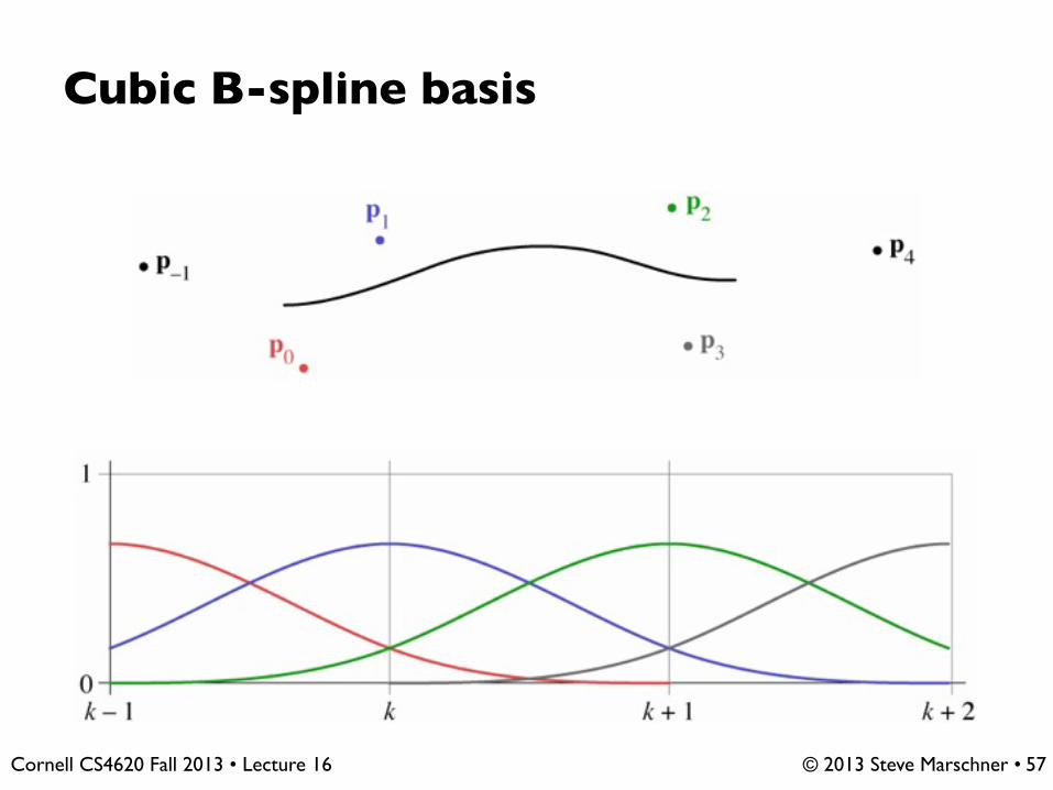
Cubic B-spline basis
57
© 2013 Steve Marschner • Cornell CS4620 Fall 2013 • Lecture 16
Cubic B-spline basis
57
© 2013 Steve Marschner • Cornell CS4620 Fall 2013 • Lecture 16
Deriving the B-Spline
• Approached from a different tack than Hermite-style constraints– Want a cubic spline; therefore 4 active control points
– Want C2 continuity– Turns out that is enough to determine everything
58
© 2013 Steve Marschner • Cornell CS4620 Fall 2013 • Lecture 16
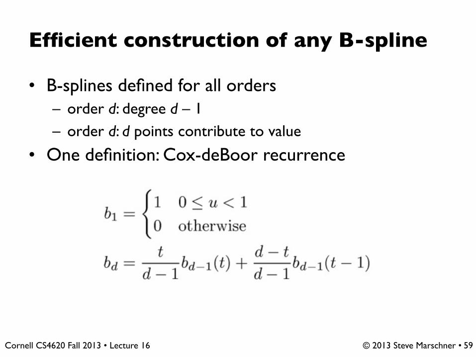
Efficient construction of any B-spline
• B-splines defined for all orders– order d: degree d – 1– order d: d points contribute to value
• One definition: Cox-deBoor recurrence
59
© 2013 Steve Marschner • Cornell CS4620 Fall 2013 • Lecture 16
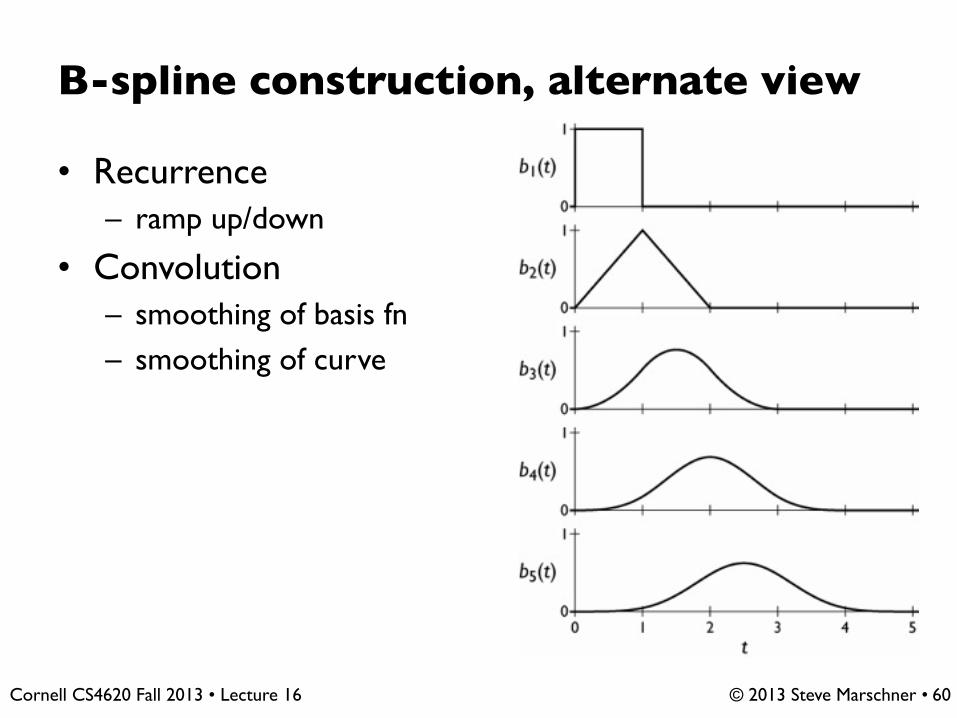
B-spline construction, alternate view
• Recurrence– ramp up/down
• Convolution– smoothing of basis fn– smoothing of curve
60
© 2013 Steve Marschner • Cornell CS4620 Fall 2013 • Lecture 16
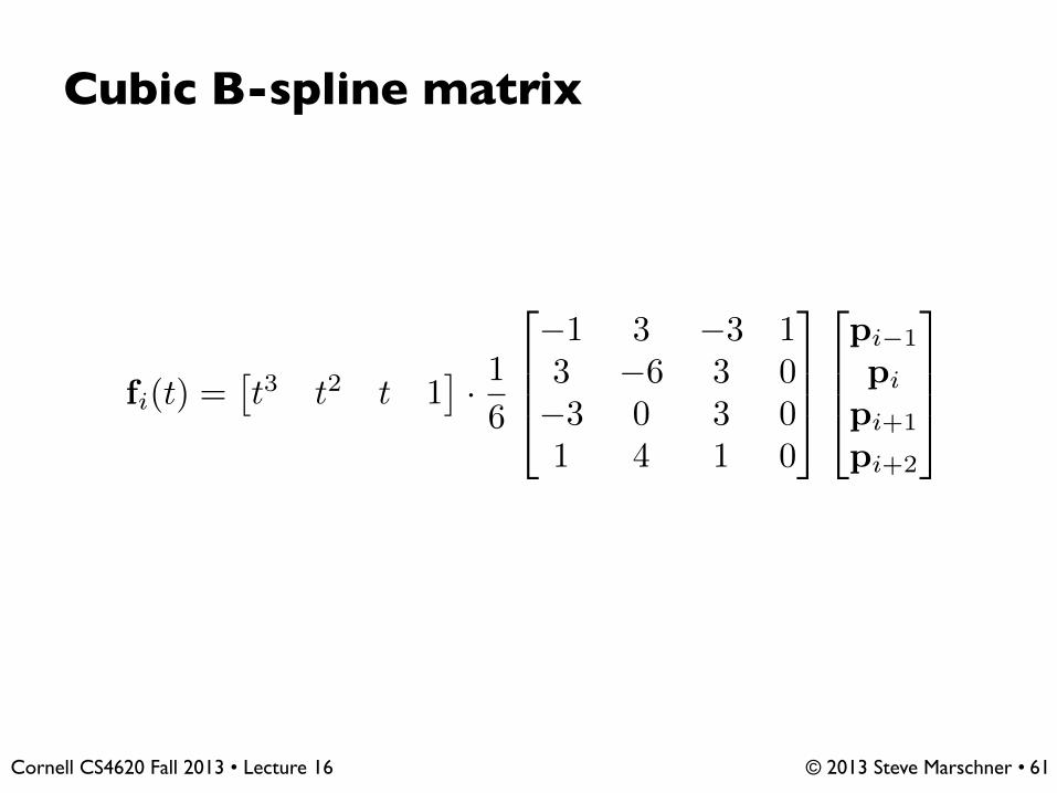
Cubic B-spline matrix
61
fi(t) =⇥t3 t2 t 1
⇤· 16
2
664
�1 3 �3 13 �6 3 0�3 0 3 01 4 1 0
3
775
2
664
pi�1
pi
pi+1
pi+2
3
775

© 2013 Steve Marschner • Cornell CS4620 Fall 2013 • Lecture 16
Converting spline representations
• All the splines we have seen so far are equivalent– all represented by geometry matrices
• where S represents the type of spline– therefore the control points may be transformed from one
type to another using matrix multiplication
62

© 2013 Steve Marschner • Cornell CS4620 Fall 2013 • Lecture 16
Refinement of splines
• May want to add more control to a curve• Can add control by splitting a segment into two
63
s
0p0
p1
p2
p3
p3
p0
p1p2
p0
p1p2
p31
find left and right control pointsto make the curves match!
f(t) = T (t)MP
fL(t) = f(st) = T (t)MPL
fR(t) = f((1� s)t+ s) = T (t)MPR

© 2013 Steve Marschner • Cornell CS4620 Fall 2013 • Lecture 16
Refinement math
64
SL =
2
664
s3
s2
s1
3
775
SR =
2
664
s3
3s2(1� s) s2
3s(1� s)2 2s(1� s) s(1� s)3 (1� s)2 (1� s) 1
3
775
fL(t) = T (st)MP = T (t)SLMP
= T (t)M(M�1SLMP )
= T (t)MPL
PL = M�1SLMP
PR = M�1SRMP
© 2013 Steve Marschner • Cornell CS4620 Fall 2013 • Lecture 16
Other types of B-splines
• Nonuniform B-splines– discontinuities not evenly spaced– allows control over continuity or interpolation at certain
points– e.g. interpolate endpoints (commonly used case)
• Nonuniform Rational B-splines (NURBS)– ratios of nonuniform B-splines: x(t) / w(t); y(t) / w(t)– key properties:
• invariance under perspective as well as affine• ability to represent conic sections exactly
65
© 2013 Steve Marschner • Cornell CS4620 Fall 2013 • Lecture 16
Evaluating splines for display
• Need to generate a list of line segments to draw– generate efficiently– use as few as possible– guarantee approximation accuracy
• Approaches– recursive subdivision (easy to do adaptively)– uniform sampling (easy to do efficiently)
66
© 2013 Steve Marschner • Cornell CS4620 Fall 2013 • Lecture 16
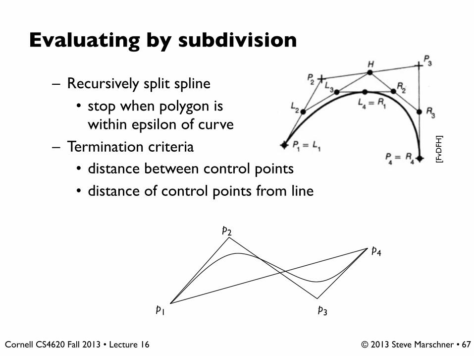
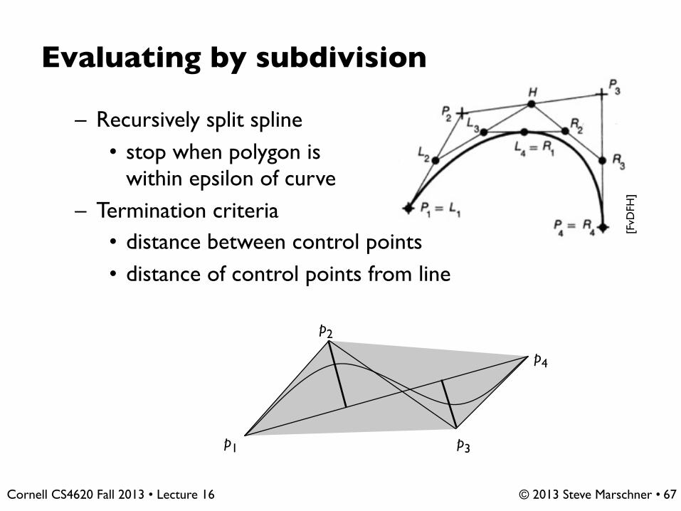
Evaluating by subdivision
– Recursively split spline • stop when polygon is
within epsilon of curve– Termination criteria
• distance between control points• distance of control points from line
p1
p2
p3
p4
[FvD
FH]
67
© 2013 Steve Marschner • Cornell CS4620 Fall 2013 • Lecture 16
Evaluating by subdivision
– Recursively split spline • stop when polygon is
within epsilon of curve– Termination criteria
• distance between control points• distance of control points from line
p1
p2
p3
p4
[FvD
FH]
67

© 2013 Steve Marschner • Cornell CS4620 Fall 2013 • Lecture 16
Evaluating with uniform spacing
• Forward differencing– efficiently generate points for uniformly spaced t values– evaluate polynomials using repeated differences
68
Top Related