


![GB5 mix design high-performance - Sabita...- Compacting ability [NF EN 12697-31]: Gyratory compactor - Moisture resistance [NF EN 12697-12]: Duriez test - Rutting resistance at 60°C](https://static.fdocuments.in/doc/165x107/60c8683095d8fe32f1212707/gb5-mix-design-high-performance-compacting-ability-nf-en-12697-31-gyratory.jpg)

Languages
Pages
Legal


EVALUATION OF THE EFFECTS OF MIXTURE PROPERTIES
AND COMPACTION METHODS ON THE PREDICTED
PERFORMANCE OF SUPERPAVE MIXTURES
by
N. Paul Khoslaand
S. Sadasivam
HWY-2001-03
FINAL REPORTFHWA/NC/2002-030
in Cooperation with
North Carolina Department of Transportation
Department of Civil Engineering
North Carolina State University
August 2002

i
Technical Report Documentation Page1. Report No.
FHWA/NC/2002-0302. Government Accession No. 3. Recipient’s Catalog No:
5. Report DateAugust 2002
4. Title and SubtitleEvaluation of the Effects of Mixture Properties and CompactionMethods on the Predicted Performance of Superpave Mixtures 6. Performing Organization Code
7. AuthorsN. Paul Khosla, S. Sadasivam
8. Performing Organization Report No.
10. Work Unit No. (TRAIS)9. Performing Organization Name and AddressDepartment of Civil EngineeringNorth Carolina State UniversityBox 7908, Raleigh, NC, 27695-7908
11. Contract or Grant No.
13. Type of Report and Period CoveredFinal ReportJuly 2001- June 2002
12. Sponsoring Agency Name and AddressNC Department of TransportationResearch and Analysis Group1 South Wilmington StreetRaleigh, NC 27601
14. Sponsoring Agency Code2001-03
15. Supplementary Notes
16.AbstractThe Superpave volumetric design method contains no strength or ‘proof’ test for quality control and quality assurance ofmixtures. Accelerated wheel tracking systems, such as the Asphalt Pavement Analyzer (APA) and the NCSU Wheel TrackingDevice (WTD) may fulfill the need for a relatively simple and inexpensive performance test. It is imperative that thepredictability of these test systems should correlate with the field performance. Moreover, several compaction methods are usedto fabricate specimens for performance testing in the laboratory. The compaction methods adopted in the laboratory areexpected to simulate the properties of the pavement in the field. It is essential that the laboratory compaction of specimensshould be a true indicator of field performance. So, the effects of different compaction methods on the performance of mixtureshave been investigated in this study.Laboratory compaction methods such as Superpave Gyratory Compaction (SGC) and Rolling Wheel Compaction (RWC) werecompared with the field compaction. Four field sites had been selected for this purpose. The mixtures were identified as AuburnCoarse, Auburn Fine, Charlotte and Kinston. The Auburn mixtures were 12.5mm mixtures whereas the Charlotte and theKinston mixtures were 9.5mm mixtures. The performance parameters of the mixtures include fatigue and rutting distresses.Various performance evaluation tests were conducted on the field cores and specimens fabricated using the Superpave GyratoryCompactor (SGC) and Rolling Wheel Compactor (RWC). Performance evaluation was done using test systems such as Sheartester, Asphalt Pavement Analyzer (APA) and NCSU Wheel Tracking Device.The analysis of test results indicate that the laboratory compacted mixtures tend to be superior in their performance than thefield cores. The mixtures compacted using the SGC and the RWC have higher stiffness values and lower shear strain valuesthan the field cores. The Rolling Wheel Compaction (RWC) seems to simulate field compaction better than the SGC. Themixtures, which failed to satisfy the RSCH test criteria, had rut depths greater than 0.5 inch, as measured by the APA andNCSU WTD. The mixtures that passed the RSCH tests had rut depths less than 0.5 inch. The APA test and the NCSU WTDtest can be used as a simulator to examine the rutting susceptibility of a mixture. It is suggested that a rut depth of 0.5 inchcould be prescribed in the APA test and the NCSU WTD test as “pass/fail” or “go no-go” criteria.
17. Key WordsSuperpave mixtures, Compaction methods, AsphaltPavement Analyzer, NCSU Wheel Tracking Device,Rutting, Fatigue Cracking
18. Distribution Statement
19.Security Classif.(of this report)Unclassified
20.Security Classif.(of this page)Unclassified
21.No. of Pages166
22.Price
Form DOT F 1700.7 (8-72)

ii
DISCLAMIER
The contents of this report reflect the views of the authors and not necessarily the views
of the University. The authors are responsible for the facts and the accuracy of the data
presented herein. The contents do not necessarily reflect the official views or policies of
either the North Carolina Department of Transportation or the Federal Highway
Administration at the time of publication. This report does not constitute a standard,
specification, or regulation.
iii
ACKNOWLEDGMENTS
The author expresses his sincere appreciation to the authorities of the North Carolina
Department of Transportation for making available the funds needed for this research.
Sincere thanks go to Mr. Cecil Jones, Chairman, Technical Advisory Committee, for his
interest and helpful suggestions through the course of this study. Equally, the
appreciation is extended to other members of the committee, Mr. Jim Grady, Mr. Carson
Clippard, Mr. Jack Cowsert, Mr. J. Travis, and Dr. Moy Biswas for their continuous
support during this study.

iv
EXECUTIVE SUMMARY
The Superpave volumetric design method contains no strength or ‘proof’ test for quality
control and quality assurance of mixtures. Accelerated wheel tracking systems, such as
the Asphalt Pavement Analyzer (APA) and the NCSU Wheel Tracking Device (WTD)
may fulfill the need for a relatively simple and inexpensive performance test. It is
imperative that the predictability of these test systems should correlate with the field
performance.
Moreover, several compaction methods are used to fabricate specimens for performance
testing in the laboratory. The compaction methods adopted in the laboratory are expected
to simulate the properties of the pavement in the field. The physical properties of the
specimens depend on the method of compaction used for fabrication. It is essential that
the laboratory compaction of specimens should be a true indicator of field performance.
So, the effects of different compaction methods on the performance of mixtures have
been investigated in this study.
Laboratory compaction methods such as Superpave Gyratory Compaction (SGC) and
Rolling Wheel Compaction (RWC) were compared with the field compaction. Four field
sites had been selected for this purpose. The mixtures were identified as Auburn Coarse,
Auburn Fine, Charlotte and Kinston. The Auburn mixtures were 12.5mm mixtures
whereas the Charlotte and the Kinston mixtures were 9.5mm mixtures. The performance
parameters of the mixtures include fatigue and rutting distresses. Various performance

v
evaluation tests were conducted on the field cores and specimens fabricated using the
Superpave Gyratory Compactor (SGC) and Rolling Wheel Compactor (RWC).
Performance evaluation was done using test systems such as Shear tester, Asphalt
Pavement Analyzer (APA) and NCSU Wheel Tracking Device. The results of these test
systems were compared and correlated. The compaction characteristics of the mixtures
were studied using the Superpave Gyratory Compactor and the Gyratory Load-Cell Plate
Assembly (GLPA).
The analysis of test results indicate that the laboratory compacted mixtures tend to be
superior in their performance than the field cores. The mixtures compacted using the
SGC and the RWC have higher stiffness values and lower shear strain values than the
field cores. The Rolling Wheel Compaction (RWC) seems to simulate field compaction
better than the SGC. There exists a good correlation among the results of the Repeated
Shear tests at Constant Height tests, the APA tests and the NCSU WTD rut tests. The
mixtures, which failed to satisfy the RSCH test criteria, had rut depths greater than 0.5
inch, as measured by the APA and NCSU WTD. The mixtures that passed the RSCH
tests had rut depths less than 0.5 inch. The APA test and the NCSU WTD test can be
used as a simulator to examine the rutting susceptibility of a mixture. It is suggested that
a rut depth of 0.5 inch could be prescribed in the APA test and the NCSU WTD test as
“pass/fail” or “go no-go” criteria.

vi
TABLE OF CONTENTS
Chapter 1: Introduction 1
1.1 Objectives and Scope of Study 3
1.2 Research Methodology and Approach 3
1.3 Summary 11
Chapter 2: Literature Review 13
2.1 Evaluation of Laboratory Compaction Methods 13
2.1.1 Compaction 13
2.1.2 Different Types of Compaction Methods 14
2.1.3 Studies on different Compaction Methods 17
2.1.4 Effect of Compaction on the Internal Structure 22
2.1.5 SGC Compaction Characteristics of Mixtures 28
2.2 Accelerated Wheel Tracking Devices 29
2.2.1 Loaded Wheel Testers used in the United States 29
2.2.2 Effect of Test Parameters and Mixture Properties on LWT Results 39
2.2.3 LWT Results Versus Field Performance 41
Chapter 3: Mixture Information 47
3.1 Field Specimens 47
3.2 Loose Mixtures 49
3.3 Characteristics of Mixtures 50

vii
3.3.1 Auburn Coarse 50
3.3.2 Auburn Fine 52
3.3.3 Charlotte 53
3.3.4 Kinston 54
Chapter 4: Compaction Characteristics of Mixtures 56
4.1 Superpave Gyratory Compactor 56
4.2 SGC Compaction of Mixtures 58
4.2.1 Compaction Characteristics 59
4.2.2 Compaction using Pine SGC 63
4.3 Gyratory Load Cell Plate Assembly 64
4.3.1 Description of GLPA 65
4.4 Energy Indices 67
Chapter 5: Performance Evaluation of Mixtures 76
5.1 Performance Evaluation using the Simple Shear Tester 76
5.1.1 Specimen Preparation 76
5.1.2 Selection of Test Temperature for FSCH and RSCH 77
5.1.3 Frequency Sweep Test at Constant Height 77
5.1.3.1 Analysis of FSCH Test Results 78
5.1.4 Repeated Shear Test at Constant Height 87
5.1.4.1 Analysis of RSCH Test Results 88
5.2 Asphalt Pavement Analyzer for Rutting Susceptibility 93

viii
5.2.1 Viscoelastic Models 100
5.3 Wheel Tracking Test 108
5.3.1 Description of NCSU WTD 108
5.3.2 Rolling Wheel Compaction of Slabs 113
5.3.3 Rutting Tests using the WTD 115
Chapter 6: Mixture Performance Analysis 123
6. 1 SUPERPAVE Fatigue Model Analysis 123
6.2 SUPERPAVE Rutting Model Analysis 132
6.3 Correlation of APA Test Results 136
Chapter 7: Summary of Results and Conclusions 143
References 154

1
CHAPTER 1
INTRODUCTION
As asphalt concrete mixture design evolved from the conventional Marshall method to
the new Superpave procedure, it became necessary to identify practical and relatively
economical laboratory methods to predict the performance of mixtures on the roadway.
Currently, the Superpave volumetric design method contains no strength or ‘proof’ test
for quality control and quality assurance of mixtures. Test procedures that are used in the
Superpave intermediate and complete procedures are designed to obtain input parameters
for the Superpave computer model and require expensive and complex test equipment.
Accelerated wheel tracking systems, such as the Asphalt Pavement Analyzer (APA), may
fulfill the need for a relatively simple and inexpensive performance test. The APA is a
thermostatically controlled device designed to predict the rutting susceptibility of the
HMA under the wheel-path by applying linear repetitive loads. Several different
laboratory compaction methods can be used to fabricate specimens for APA testing
including the Superpave gyratory compactor (SGC), vibratory, static and rolling wheel.
Each of these methods may produce specimens that have very different aggregate particle
orientation, voids and corresponding estimated performance. For the APA to be used for
performance testing, it is imperative that the specimens tested in this device be
representative of the mixtures as they exist in the field.
As the use of Superpave mixtures increases, so will experience in their design and
construction. It is thought that Superpave mixtures are generally more difficult to

2
compact than Marshall mixtures in some cases. One possible reason for this is the wide
range of properties and physical characteristics of the aggregates and binder types used in
different geographic regions of the country. The compaction level and volumetric
specifications in Superpave may be difficult to achieve or even unnecessary in some
locations of the United States. It may be essential for state highway agencies to modify or
amend the Superpave design specifications to cover the traffic levels, source material
properties and observed performance in their jurisdictions. For instance, the design
compaction level used by the SGC (as given by Ndes and Nmax) should be evaluated by
observing how the designed mixtures compact in the field and perform in laboratory
evaluation equipment.
With respect to the performance evaluation of Superpave mixtures used in North
Carolina, several questions may be posed,
1. How well do specimens fabricated used laboratory compaction methods simulate the
properties of the pavements in the field ?
2. Can the densification curves generated by the SGC (Ndes and Nmax) during the mixture
design process be compared to the field densities of the mixes ?
3. Can a performance evaluation device such as the APA be used to detect poorly
performing Superpave mixtures ?
4. How does mixture performance as measured by the APA correlate with that of other
performance evaluation procedures and devices ?

3
The following sections describe the proposed objectives and approach that will be used to
explore the answers to these questions.
1.1 Objectives and Scope of Study
In order to address the concerns and questions presented above, the primary objectives of
this study are:
1. Evaluate the effects of compaction type (rolling wheel and Superpave gyratory
compactor) on a mixture’s performance as measured by the APA, Wheel Tracking
Device at NCSU and Repeated Shear Constant Height test (RSCH).
2. Evaluate how changes in aggregate and asphalt source affect mixture compaction
and predicted performance in the test systems listed in 1 above by employing several
Superpave mixtures from different field sites in North Carolina.
3. Compare the predicted performance, as measured by the test systems listed above, of
test samples compacted in the field to the same mixtures compacted using the
laboratory compaction systems listed in 1.
4. Evaluate and compare the densification characteristics of mixtures with varying
degree of compaction (in terms of number of gyrations) in the Superpave Gyratory
Compactor (SGC) and the Gyratory Load Cell Plate Assembly (GLPA).
1.2 Research Methodology and Approach
The research plan consisted of three main tasks. First, the field sites were selected from
which test samples were collected. Secondly, loose mixtures from these sites were
compacted using Rolling Wheel Compactor (RWC) and Superpave Gyratory Compactor

4
(SGC). Lastly, the performance of these laboratory compacted mixtures was compared to
the performance of the field cores and slabs obtained from the selected sites. A more
detailed explanation of this work plan is given in Figure 1.1.
Figure 1.1 Research Plan
Task 1: Field Site Selection and Test Material Procurement
Since one of the objectives of this research was to evaluate how changes in aggregate and
binder sources affect the performance evaluation of mixtures, typical mixtures were
selected from different geographic regions in and out of North Carolina. Field specimens
and loose mixtures were collected from these sites.
Task 1.1 Site Selection:
The location and the total number of test sites were selected after consultation with
NCDOT. Four test sites were selected in such a way that each test site had a different
type of aggregate gradation (coarse or fine) and a nominal maximum size of aggregate
Field Mixtures Test Systems Lab Compaction
Field Cores
Field Slabs
Shear Tester
APA
NCSU WTD
GLPA
Rolling WheelCompaction
SuperpaveGyratory
Compaction

5
(12.5mm or 9.5mm). The test sites were Auburn (NCAT research tracks), Kinston and
Charlotte. NCDOT was the contractor for the North Carolina test sections in NCAT
research tracks. The Kinston and the Charlotte mixtures were from Kinston and
Matthews counties of North Carolina. The aggregate sources for all the four mixtures
were from the quarries of North Carolina. The detailed information about the mixtures is
provided in the following chapters. These sites were the pavements that contain
SUPERPAVE volumetrically designed mixtures being used in either new or overlay
construction.
Task 1.2 Test Sample Procurement:
After the number and location of test sites were selected, test samples were gathered from
each site. Test samples included field cores, field slabs and loose mixtures. Loose
mixtures were procured for the compaction of the mixtures using SGC and Rolling
Wheel compactor. Field cores and loose mixtures were taken from all the four sites,
whereas field slabs were available only for the Kinston and the Charlotte mixtures. Field
cores were 150 mm in diameter with varied thickness. The thicknesses of field slabs were
75mm and 100mm for the Kinston and the Charlotte mixtures, respectively.
Task 2: Evaluation of Laboratory Compaction Methods
The central objective of this research was to evaluate how different compaction methods
(RWC and SGC) differ from the field compaction in performance, say fatigue and rut
life. The following subsections outline how each of these compaction methods was used
to accomplish this phase of research.

6
Rolling Wheel Compaction using the NCSU Wheel Tracking Device:
The Wheel Tracking Device (WTD) at NCSU has the ability to compact large rectangular
slab samples using a steel rolling wheel at various compaction pressures. The sample size
used in the WTD is 520mm long, 430mm wide and up to a thickness of 300mm in 75mm
lifts. Since the WTD rolling wheel compactor has been scaled and designed to match that
of field compaction equipment, it is thought that it simulates field compaction better than
any other laboratory compaction method currently in use.
Cylindrical test specimens were cored out from the RWC slabs for repeated shear tests
and APA tests. The test results of RWC specimens were then compared with the
corresponding results of field cores and SGC compacted specimens. The rutting
performance of rolling wheel compacted mixtures was evaluated by using accelerated test
facility in the WTD and the results were compared to those from the APA.
Superpave Gyratory Compactor:
The SGC was used to fabricate cylindrical test specimens, with densities similar to those
of the field mixtures, for testing in the SST and the APA. The rutting performance of
these samples were compared to the samples compacted by the other laboratory methods
and field cores. In addition to the use of the SGC as a compaction method for testing in
the SST and the APA, one of the objectives of this study was to compare how the
compaction curve of the SGC compares to the actual field density of the mixtures. Since
the gyratory compactor is used to fabricate mixtures in the SUPERPAVE volumetric

7
design procedure, Ndes should correspond to a mixture’s field density after construction,
while the %Gmm should be 96%. The level of relative compaction in the SGC can be
verified or calibrated for the design of SUPERPAVE mixtures used in North Carolina.
This is also another reason why the evaluation of field sites using the SUPERPAVE
volumetrically designed mixtures in new or overlay construction would be beneficial to
this study.
The compaction characteristics of the mixtures were studied and compared to the results
from the Gyratory Load Plate Assembly (GLPA). The energy indices measured using the
GLPA and the SGC better explains the compaction characteristics of the mixtures during
construction and under traffic.
Task 3: Performance Evaluation
As discussed above, the relative rutting performance of samples fabricated using the
laboratory compaction methods were compared to each other and to the rutting
performance of the samples taken from the field. The objective being to determine which
compaction method yields a sample that exhibits similar performance to that produced in
the field. The last phase of research was to evaluate the APA itself in order to calibrate
the rutting performance it predicts to that of two other rutting evaluation tests: the NCSU
wheel tracking device and the simple shear tester.

8
Asphalt Pavement Analyzer:
The APA basically consists of three parallel steel wheels, rolling on a pressurized rubber
tube, which applies loading to beam or cylindrical specimens in a linear track. The test
specimens, loading tubes and wheels are all contained in a thermostatically controlled
environmental chamber. The depth of rutting in the test specimens is measured after the
application of 8000 loading cycles. The predicted rutting measured by the APA is the
central facet of the study. As mentioned above, Task 2 was to evaluate how the
performance of sample fabricated using different laboratory compaction methods
compared to that of the field specimens. The results of the APA tests were compared with
the results of the Simple Shear Tester and the WTD at NCSU.
Simple Shear Tester:
The SST is a closed-loop system that consists of four major components: the testing
apparatus, the test control unit and data acquisition system, the environmental control
chamber, and the hydraulic system. In this proposed study, repeated shear test at constant
height and frequency sweep test at constant height was used to analyze the performance
of HMA mixtures. A full description of the test procedures can be found in AASHTO
TP7. The rutting and fatigue analyses were then conducted using the test results.
The frequency sweep test at constant height was used to analyze the permanent
deformation and fatigue cracking. A repeated shearing load was applied to the specimen
to achieve a controlled shearing strain of 0.045 percent. The specimen was tested at each
9
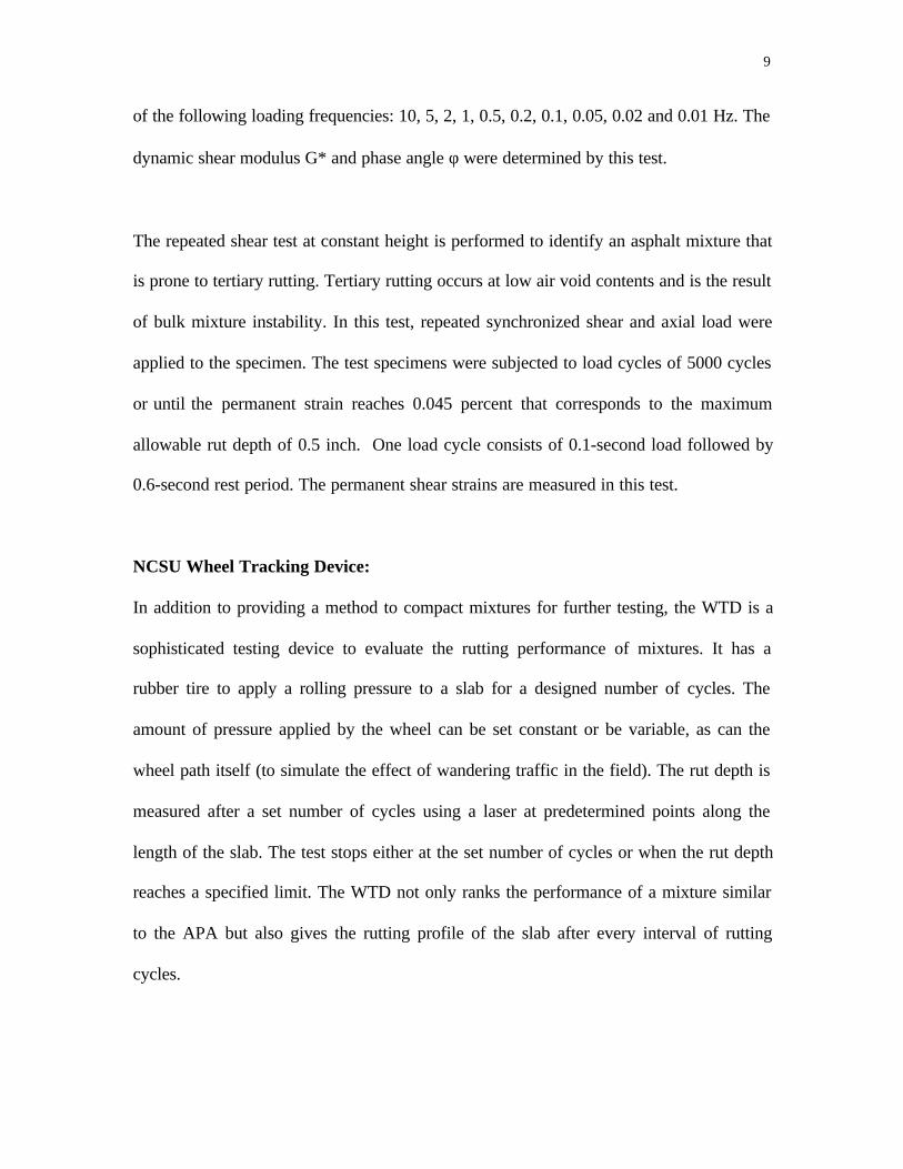
of the following loading frequencies: 10, 5, 2, 1, 0.5, 0.2, 0.1, 0.05, 0.02 and 0.01 Hz. The
dynamic shear modulus G* and phase angle φ were determined by this test.
The repeated shear test at constant height is performed to identify an asphalt mixture that
is prone to tertiary rutting. Tertiary rutting occurs at low air void contents and is the result
of bulk mixture instability. In this test, repeated synchronized shear and axial load were
applied to the specimen. The test specimens were subjected to load cycles of 5000 cycles
or until the permanent strain reaches 0.045 percent that corresponds to the maximum
allowable rut depth of 0.5 inch. One load cycle consists of 0.1-second load followed by
0.6-second rest period. The permanent shear strains are measured in this test.
NCSU Wheel Tracking Device:
In addition to providing a method to compact mixtures for further testing, the WTD is a
sophisticated testing device to evaluate the rutting performance of mixtures. It has a
rubber tire to apply a rolling pressure to a slab for a designed number of cycles. The
amount of pressure applied by the wheel can be set constant or be variable, as can the
wheel path itself (to simulate the effect of wandering traffic in the field). The rut depth is
measured after a set number of cycles using a laser at predetermined points along the
length of the slab. The test stops either at the set number of cycles or when the rut depth
reaches a specified limit. The WTD not only ranks the performance of a mixture similar
to the APA but also gives the rutting profile of the slab after every interval of rutting
cycles.

10
Frictional Resistance by Gyratory Load Cell Plate Assembly:
A Gyratory Load Cell Plate Assembly (GLPA) was developed and initially tested at the
University of Wisconsin – Madison. This device easily fits on most SGCs without
modification and requires no deviation in the compaction procedure. The assembly
consists of three load cells fixed between two parallel plates at an equal radial distance,
120o apart. The force on the three load cells is continuously monitored, along with sample
deflection and height, throughout the fabrication process. The corresponding resultant
force and eccentricity acting on the plates are then calculated. Assuming that at any
gyration the sample is fully constrained, and the energy due to surface traction is
negligible, the energy balance for the sample can be written using the following:
W = U (1.1)
Where
W = work of the external forces, and
U = total strain energy of the sample
Expanding the above equation yields the following:
½ Mθ= ½ τγV (1.2)
where,
M = applied moment,
θ = tilt angle (radians)
τ = frictional resistance
γ = shear strain
V = sample volume at any cycle

11
The resulting moment M can be calculated by multiplying the ram force R by the
eccentricity e for a given gyration cycle. The frictional resistance can be determined by
simplifying the above equation into the form
τ = FR = Re/Ah (1.3)
where,
A = sample cross section area
H = specimen height at any given gyration
The University of Wisconsin study found that asphalt content, aggregate gradation,
aggregate angularity, air voids and compaction temperature all affected the frictional
resistance of the specimen, and recommendations were made concerning the use of
%Gmm with frictional resistance in the mixture design process. However, no correlations
were made between frictional resistance, other mixture performance equipment or
methods, and actual field performance. In view of the above discussion, GLPA was used
in this study to determine the potential of such a device to provide a measure of stability
of asphalt mixtures. Furthermore, it offered an opportunity to see if the frictional
resistance in the laboratory evaluation had any relationship to field performance.
1.3 Summary
• Four types of mixtures were selected for this study from different geographic
locations in and out of North Carolina to study the effects of aggregate and binder

12
type on the compaction of mixtures. Field slabs, field cores, and loose mixtures were
procured from these test sites. The mixture densification information of mixtures was
obtained.
• The laboratory compaction methods included the WTD rolling wheel compactor and
the Superpave Gyratory Compactor. The cylindrical specimens fabricated using these
compactors were tested using the SST and the APA. The test results were compared
to the test results of field cores. Similarly the WTD rut test results of rolling wheel
compacted slabs were compared to those of field slabs. The densification information
generated by the SGC and the energy indices developed using the SGC and GLPA
explained the compaction characteristics of the mixtures.
• The relative rutting measurements obtained by the performance testing devices were
also compared.

13
CHAPTER 2
LITERATURE REVIEW
This chapter reviews the background literature that deals with the effect of different
compaction methods, different types of accelerated laboratory wheel tracking devices and
the performance of the Asphalt Pavement Analyzer (APA).
2.1 Evaluation of Laboratory Compaction Methods
The objective of a mix design system has always been to mix, compact, and test asphalt
mixtures in the laboratory to determine its expected performance in service. The
specimen prepared in the laboratory should be representative of a field-compacted
specimen having the same properties as the prototype placed in the field and subjected to
the compactive effects of traffic. So it is irrefutable that the laboratory compaction of
specimens should be a true indicator of field performance. This section compares the
various laboratory compaction methods and their ability to simulate field densification.
2.1.1 Compaction
Pavement density is a function of traffic and climate (temperature). For pavements to be
designed correctly, traffic and climate must be simulated in the laboratory for mix design.
The heart of all mixture design methods is the laboratory compaction method (1).
RILEM 152 PBM (2) identifies the type and degree of compaction as one of the five
preparatory steps in the basic testing methodology of bituminous mixture design.
Compaction of an asphalt concrete mixture is defined as “…a stage of construction,
14
which transforms the mix from its very loose state into a more coherent mass, thereby
permitting it to carry traffic loads”. The efficiency of the compactive effort will be a
function of the internal resistance of the bituminous concrete. The resistance includes
aggregate interlock, friction resistance, and viscous resistance. Another reason for
compacting the asphalt pavement is to make it water tight and impermeable to air.
From the Hubbard Field method of mix design to the SHRP SUPERPAVE method,
attempts have been made to select a compaction method that closely duplicates the
properties of the actual road pavement. It is well established that method of compaction
affects the physical properties of compacted asphalt concrete specimens. Factors such as
particle orientation and aggregate interlock, void structure, and the number of
interconnected voids should be considered in the selection of a compaction device (3).
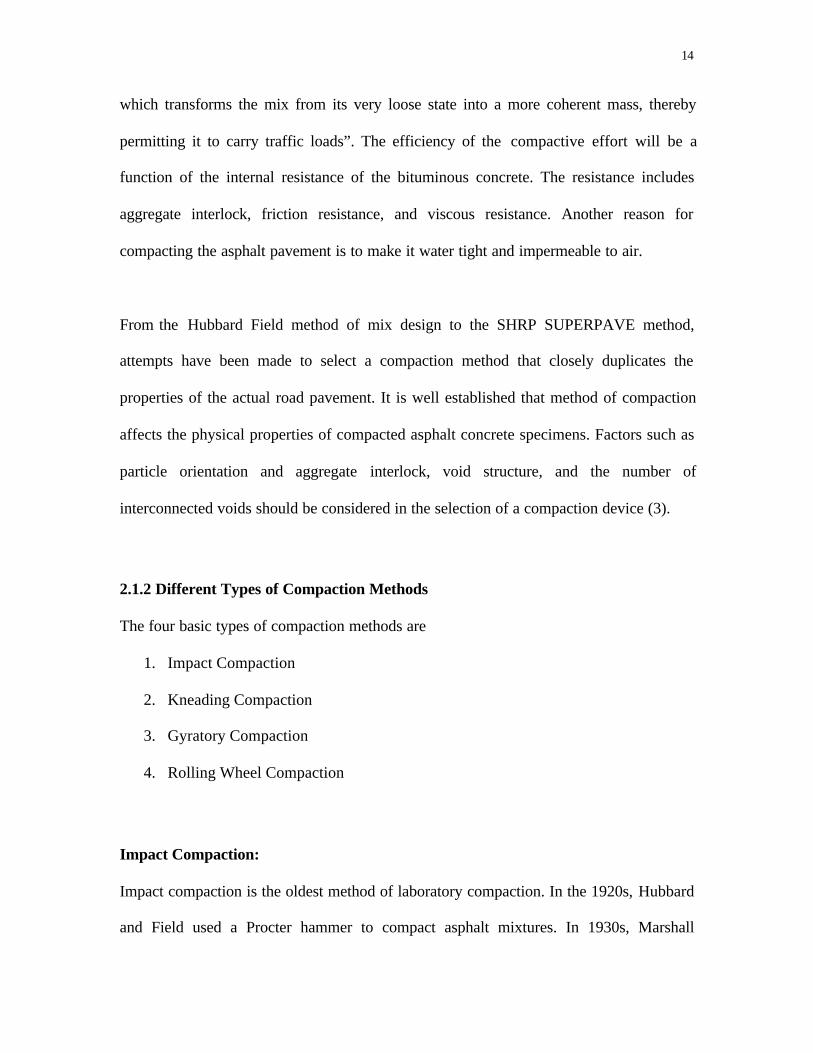
2.1.2 Different Types of Compaction Methods
The four basic types of compaction methods are
1. Impact Compaction
2. Kneading Compaction
3. Gyratory Compaction
4. Rolling Wheel Compaction
Impact Compaction:
Impact compaction is the oldest method of laboratory compaction. In the 1920s, Hubbard
and Field used a Procter hammer to compact asphalt mixtures. In 1930s, Marshall

15
developed mechanical Marshall Hammer to simulate impact type compaction. The
number of blows applied to each face of the specimen (35, 50 and 75 blows) was tied to
general traffic levels. Higher energy levels (blows) were used for higher traffic levels.
Unfortunately, different densities, because of the variability in Marshall hammers
(mechanical, rotating, and manual hammers), will result when these compaction blows
are applied (1).
Kneading Compaction:
The compaction method used by Hveem in his mix design procedure is kneading
compaction. Kneading compaction applies forces through a roughly triangular-shaped
foot that covers only a portion of the specimen face. Compacted forces by tamps are
applied uniformly on the free face of specimen to achieve compaction. The partial face
allows particles to move relative to each other, creating a kneading action that densifies
the mix. There are different kneading compactors like California kneading compactor,
Linear kneading compactor (LKC) and Arizona kneading compactor (1).
Gyratory Compaction:
Gyratory compaction was developed in the 1930s in Texas. Later this method of
compaction was further developed and applied by the Army Cops of Engineers and the
Central Laboratory for Bridges and Roads (LCPC) in France. One of the final product of
Strategic Highway Research Program (SHRP) was Superpave Gyratory Compactor.
Other types of gyratory compactors (4) are
§ Texas Roots of Gyratory Compaction

16
§ Corps of Engineers Gyratory Testing Machine
§ LCPC French Gyratory Compaction
Gyratory process involves applying a vertical load while gyrating the mold in a back-and
forth motion. Gyratory compaction produces a kneading action on the specimen.
Superpave Gyratory Compactor
The decision to use gyratory compaction as the Superpave compaction is based on
NCHRP Study 9-5. NCHRP 9-5, which was designed to be a lead-in to the SHRP,
focused on compaction methods and developed a preliminary mix design and analysis
system using pre-SHRP performance related tests. Midway through the SHRP, as the
Superpave method of mix design was being assembled, an evaluation of available
gyratory compaction research was done.
An underlying premise of the gyratory protocol selection was that material property
parameters were not expected to come from the compactor. The primary objective of
SHRP was to develop and validate material properties, and test methods to measure the
properties, which could be used to predict performance. Therefore, the need for
fundamental or empirical engineering properties from a compactor did not exist. Hence,
the material properties, which can be measured with the Gyratory Testing Machine, were
not required.
The ability to evaluate the rate of densification was selected as a desirable characteristic.
The constant angle and constant vertical pressure of the Texas 6 inch gyratory allowed
17
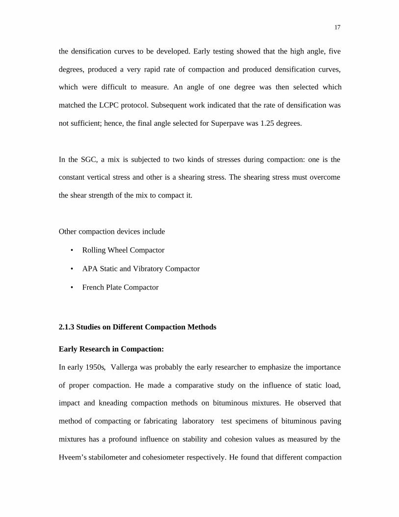
the densification curves to be developed. Early testing showed that the high angle, five
degrees, produced a very rapid rate of compaction and produced densification curves,
which were difficult to measure. An angle of one degree was then selected which
matched the LCPC protocol. Subsequent work indicated that the rate of densification was
not sufficient; hence, the final angle selected for Superpave was 1.25 degrees.
In the SGC, a mix is subjected to two kinds of stresses during compaction: one is the
constant vertical stress and other is a shearing stress. The shearing stress must overcome
the shear strength of the mix to compact it.
Other compaction devices include
• Rolling Wheel Compactor
• APA Static and Vibratory Compactor
• French Plate Compactor
2.1.3 Studies on Different Compaction Methods
Early Research in Compaction:
In early 1950s, Vallerga was probably the early researcher to emphasize the importance
of proper compaction. He made a comparative study on the influence of static load,
impact and kneading compaction methods on bituminous mixtures. He observed that
method of compacting or fabricating laboratory test specimens of bituminous paving
mixtures has a profound influence on stability and cohesion values as measured by the
Hveem’s stabilometer and cohesiometer respectively. He found that different compaction

18
methods gave different stability values even when the compacted mixes show the same
density. This observation made him to conclude that different compaction methods yield
different “orientation” or “arrangement” of particles that influence the stability or
resistance to deformation of the mass rather than mere ascribe to the density or decrease
in void ratio alone (5).
Studies by Von Quintus et al:
A NCHRP sponsored study evaluated the ability of five compaction devices to simulate
field compaction (6). The compaction devices evaluated were selected on the basis of
their availability, uniqueness in mechanical manipulation of mixture and potential for use
by agencies responsible for asphalt mixture design. The devices evaluated are
• Mobile steel wheel simulator
• Texas gyratory compactor
• California kneading compactor
• Marshall impact hammer
• Arizona vibratory-kneading compactor
The ability of the five laboratory compaction devices to simulate field compaction is
based on the similarity between engineering properties (resilient moduli, indirect tensile
strengths and strain at failure, and tensile creep data) of laboratory-compacted samples
and field cores. The test results show that although there is no single laboratory
compaction method that always provided the best match with the results of the field
compaction method, the Texas gyratory compactor demonstrated the ability to produce
mixtures with engineering properties nearest those determined from field cores. The
California kneading compactor and the mobile steel wheel simulator ranked second and

19
third respectively, but with very little difference between the two. The Arizona vibratory
kneading compactor and the Marshall impact hammer ranked as least effective in terms
of their ability to produce mixtures with engineering properties similar to those from field
cores.
An abstract of results are given in Table
Percent of Cells with properties
Compaction Device Closest to
Field Cores
Indifferent from the
Field Cores
Texas Gyratory
Mobile steel wheel simulator
California kneading compactor
Arizona vibratory-kneading compactor
Marshall impact hammer
45
25
23
7
7
63
49
52
41
35
Studies by Joe Button et al
A similar study was carried out by Joe W. Button et al , as a part of the research project
for SHRP program (7). Four types of compaction methods that were evaluated are
• Exxon Rolling Wheel
• Texas Gyratory compactor
• Rotating base Marshall hammer
• Elf linear kneading compactor

20
Laboratory-fabricated specimens from each compaction device were tested to
characterize the material response of each mixture in tensile and compressive shear
modes of loading. Test results were compared to corresponding results from field cores
and statistically analyzed. Analyses indicated that the gyratory method most often
produced specimens similar to pavement cores (73 percent of the tests performed). Exxon
and Elf compactors had the same probability of producing specimens similar to pavement
cores (64 percent of the tests performed). The Marshall rotating base compactor had the
least probability of producing specimens similar to pavement cores (50 percent of the
tests performed). He observed difficulties in using Exxon rolling wheel compactor in
controlling air voids with the finished specimens than the other compaction methods. He
concluded that the Texas gyratory compactor is more convenient for preparing laboratory
specimens for routine mixture design and testing of asphalt concrete. From the above
study, it seems to be rational to argue that gyratory method of compaction would provide
better results than the other compaction methods.
Studies by UCB Research Group
As a part of SHRP A-003 research program at University of California, Berkeley, Sousa
et al investigated gyratory (Texas type), kneading and rolling wheel compaction
procedures (3).
The gyratory compactor was found to place excessive emphasis on the asphalt binder and
to inaccurately portray the role of asphalt aggregate interaction in the performance of

21
properly constructed pavements. Furthermore, the shape and dimension of specimens
produced by gyratory compactors are limited. Although kneading compactor is more
adaptable for producing a larger variety of sizes and shapes, it creates a more stable
aggregate structure that is commonly developed by conventional construction practice,
thereby failing to capture the role of the asphalt binder in properly performing pavements.
Because the response of rolling wheel specimens to test loads is typically between that of
gyratory and kneading specimens, rolling wheel compaction is best suited for preparing
laboratory specimens. Among the methods investigated, it appears to duplicate field-
compacted specimens quite well.
Accordingly, based on these studies as well as an evaluation of international experience,
it is strongly recommended that rolling wheel compaction be used for the preparation of
laboratory specimens of asphalt-aggregate mixes which are to be evaluated as a part of a
comprehensive asphalt-aggregate mix analysis system.
Rolling-wheel compaction is intuitively appealing for its obvious similarity to field
compaction process. Moreover, extensive studies have demonstrated that it produces
uniform specimens with engineering properties similar to those of cores extracted from
recently constructed pavements. Rolling Wheel compaction is a comparatively easy
procedure to use and enables rapid fabrication of specimen in suitable numbers and
shapes for a comprehensive mix design/analysis system. Because specimens produced by
rolling wheel compaction are cored or sawed from a larger mass, all surfaces are cut. Cut
surfaces are desirable because air voids can be more accurately measured, comparisons

22
with specimens extracted from in-service pavements are more accurate, specimens are
more homogeneous, and test results are likely to be less variable. Rolling-wheel
compaction also has the advantage that specimens containing large-size aggregates can
be produced without difficulty.
European experience has proven the practicality and superiority of rolling wheel
compaction. It is recommended form of specimens preparation in France and is a major
component of the LCPC mix design/evaluation methodology. Studies in the United
Kingdom as well as the Royal Dutch Shell Laboratory, Amsterdam, also demonstrate the
effectiveness of rolling wheel compaction.
2.1.4 Effect of Compaction on the Internal Structure
From the above discussions, it is evident that the method of compaction has profound
influence on the measured mechanical properties on the compacted asphalt concrete
specimens. Earlier research indicate that gyratory, rolling wheel, and kneading
compaction produce specimens with significantly different permanent deformation
responses to repeated shear loading. The effect of compaction procedure has been mainly
attributed the difference in the internal structure of the compacted mixes.
Internal structure refers to the distribution of aggregates and their associated voids. The
air void distribution constitutes the first phase of the internal structure. The Superpave
volumetric mixture design procedure focuses on average percent air voids for specifying
and designing AC mixtures. Two specimens with the same average percent air voids may

23
have a different distribution of air voids and intuitively they are expected to respond
differently under loading conditions. The next aspect of the internal structure of AC is
aggregate distribution, orientation and contacts. Researchers have already established the
relationship between the number of contacts and shear strength of granular assembly.
Two different research groups have studied the effect of compaction methods on internal
structure of asphalt concrete specimens using image analysis. Digital Image Processing
(DIP) consists of converting video pictures into a digital form and applying various
mathematical procedures to extract significant information from the picture. It is fast
becoming a versatile tool for characterizing the internal structure of materials. The
research group at UCB and Danish National Roads Laboratory (DNRL) used image
analysis of plane specimens compacted using UCB rolling wheel, Texas Gyratory and
California kneading compactors (8). E.Masad et al used DIP to quantify the internal
structure parameters of specimens compacted using Superpave gyratory compactor and
linear kneading compactor (9).
Aggregate Orientation:
The results of the image analysis of Masad et al show that the aggregates have preferred
orientation toward the horizontal direction in SGC and they appear to have more of a
random distribution in Linear Kneading Compactor (LKC) specimens. The average angle
of inclination was found to be smaller for specimens compacted with the SGC than those
compacted with the LKC.

24
DRNL’s image analysis confirms the hypothesis that a greater degree of aggregate
orientation results from rolling wheel compaction as compared with that produced by the
Texas gyratory compactor. These findings support the hypothesis that Texas gyratory
specimens’ lower resistance to permanent deformation under repetitive shear loads is at
least partly related to the lack of a strong , oriented aggregate structure. On the other
hand, the rolling wheel specimens’ greater resistance is a result of aggregate orientation
and inter particle contact caused by the forces induced by the rolling alone because unlike
gyratory and kneading methods, rolling wheel compaction does not include any static
leveling loading that might increase particle-to-particle contact by crushing aggregates
together.
Contacts:
The results of the image analysis by E.Masad et al indicate that LKC specimens had more
contacts (about 550 contact points on six sections) than the SGC specimens (about 450
contact points). It is interesting to note that several studies have indicated that specimens
compacted by kneading action had significantly higher resistance to permanent
deformation than specimens compacted by gyratory action. Evidently, the higher shear
strength of kneading compacted specimens is associated with the high number of coarse
aggregate contacts.
Air void distribution:
Asphalt aggregate mixes compacted in the field usually have increasing air void contents
from the top of the lift to the bottom. The reason for air-void gradients can be easily
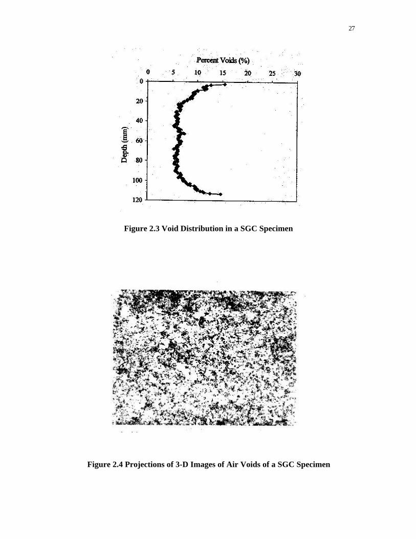
25
explained by the distribution of forces under a field compaction wheel which decrease
with depth. E.Masad et al studied the air void distribution in SGC and LKC compacted
specimens using X-ray tomography. The middle of the SGC specimen was compacted
more than the top and the bottom. For the materials studied, the air voids were found to
be relatively uniform between 20 and 100mm. In the LKC specimens, air voids were
more concentrated at the bottom (Fig.2.1-2.4).
Rolling wheel compacted specimens would be expected to have increasing air void
contents from the top to the bottom of the lift, as do field specimens. Air void contents
are expected to be fairly homogeneous in the horizontal plane of the rolling wheel.
Gyratory specimens are subjected to a high axial compressive stress, a side-to-side shear
stress, and a torsional shear stress. Under high axial compressive stresses and many
gyrations, it is expected that the interior of the specimen become better compacted. The
torsional shear stress, and the inability of aggregate to become oriented, is thought to
reduce compaction near the vertical walls of the specimen. As-compacted Texas gyratory
and kneading compacted specimens appear to have different aggregate and air void
structure near the mold surface than in their interior.
The method of compaction has a profound influence on the engineering properties of
asphalt concrete mixtures. Different methods of compaction yield different aggregate
orientation and air void distribution. Conclusions of different studies indicate that
gyratory method and rolling wheel compactions simulate properties that are closer to
field compaction.

26
Figure 2.1 Horizontal X-ray Tomography Image of a SGC Specimen
Figure 2.2 Optical Digital Camera Image of a Vertical Section of a SGC Specimen
27
Figure 2.3 Void Distribution in a SGC Specimen
Figure 2.4 Projections of 3-D Images of Air Voids of a SGC Specimen

28
2.1.5 SGC Compaction Characteristics of Mixtures
A significant component of the Superpave Volumetric mix design protocol lies on the
compaction process. The laboratory compaction process proceeds through three land
marks: Nini which corresponds to the state of the mixture as the breakdown roller makes
its first few passes; Ndes representing the anticipated state of density in the mixture after 3
to 5 years; and Nmax which represents a “factor-of-safety” condition should the traffic
projections be seriously underestimated or the climate hotter than the anticipated (10).
The densification curve (%Gmm vs. log N) would accurately represent the state of the
mixture at any point in the anticipated life of the mixture, i.e., during construction and
subsequently under traffic. Hussain U.Bahia et al (11) introduced the concept of
compaction energy indices by utilizing the SGC results to optimize the densification
characteristics under construction and densification characteristics under traffic. The
densification curves were separated into different regions to represent the construction
compaction requirements and the traffic densification to selected air voids or to terminal
densification. The compaction energy index (CEI) and the traffic densification index
(TDI) are used as new measures to relate to construction and in-service performance of
mixtures. But the rationality of the use of these indices is being questioned. Coree and
Vander Horst (10) argue that the greater part of the compaction is achieved while the
mixture is in excess of 115oC. But the mixture temperature under operating conditions
under traffic may range from -28 oC to 58 oC (as indicated by the grade of the binder, PG
58-28). Moreover they argue about the non-conformation of the SGC data to rutting
models adopted by Superpave. The inability of the SGC compaction curve to highlight
plastic instability is attributed to the fact that the mixture is so effectively contained

29
within the relatively infinitely rigid walls of the mold and equally rigid top and bottom
platens that the type of lateral flow observed in rutting pavement is totally prevented,
even though the actual state of the mixture may be wholly plastic during laboratory
compaction.
2.2 Accelerated Wheel Tracking Devices
Accelerated laboratory rutting prediction tests are needed for design as well as quality
control/quality assurance purposes. Laboratory wheel tracking devices potentially could
be used to to identify HMA mixtures that may be prone to rutting. Loaded wheel testers
(LWT) are becoming increasingly popular with transportation agencies as they seek to
identify hot mix asphalt mixtures that may be prone to rutting. The LWTs allow for an
accelerated evaluation of rutting potential in the designed mixes (12)
2.2.1 Loaded Wheel Testers used in the United States
Several LWTs currently are being used in the United States. They include the Georgia
Loaded Wheel Tester (GLWT), Asphalt Pavement Analyzer (APA), Hamburg Wheel
Tracking Device (HWTD), LCPC (French) Wheel Tracker, Purdue University
Laboratory Wheel Tracking Device (PURWheel), and one-third scale Model Mobile
Load Simulator (MMLS3). Following are descriptions for each of these LWTs.
Georgia Loaded Wheel Tester
The GLWT was developed during the mid-1980s through a cooperative research study
between the Georgia Department of Transportation and the Georgia Institute of

30
Technology. The primary purpose for developing the GLWT was to perform efficient,
effective, and routine laboratory rut proof testing and field production quality control of
HMA. The GLWT is capable of testing HMA beam or cylindrical specimens. Beam
dimensions are generally 125 mm wide, 300 mm long, and 75 mm high (5 in x 12 in x
3in). Compaction of beam specimens for testing in the GLWT has varied greatly
according to the literature. The original work by Lai (13) utilized a "loaded foot"
kneading compactor. Heated HMA was "spooned" into a mold as a loaded foot assembly
compacted the mixture. A sliding rack, onto which the mold was placed, was employed
as the kneading compactor was stationary. West et al. utilized a static compressive load to
compact specimens. Heated HMA was placed into a mold and a compressive force of 267
kN(60,000 lbs) was loaded across the top of the sample and then released.
This load sequence was performed a total of four times. In 1995, Lai and Shami
described a new method of compacting beam samples. This method utilized a rolling
wheel to compact beam specimens. Laboratories prepared cylindrical specimens are
generally 150 mm in diameter and 75 mm high. Compaction methods for cylindrical
specimens have included the "loaded foot" kneading compactor and a Superpave gyratory
compactor. Both specimen types are most commonly compacted to either 4 or 7 percent
air void content. However, some work has been accomplished in the GLWT at air void
contents as low as 2 percent (14). Testing of samples within the GLWT generally consists
of applying a 445-N (100-lb) load onto a pneumatic linear hose pressurized to 690 kPa
(100 psi). The load is applied through an aluminum wheel onto the linear hose, which
resides on the sample. Test specimens are tracked back and forth under the applied

31
stationary loading. Testing is typically accomplished for a total of 8,000 loading cycles
(one cycle is defined as the backward and forward movement over samples by the
wheel). However, some researchers have suggested fewer loading cycles may suffice.
Test temperatures for the GLWT have ranged from 35°C to 60°C (95°F to 140°F). Initial
work by Lai was conducted at 35°C (95°F). This temperature was selected because it was
Georgia's mean summer air temperature. Test temperatures within the literature
subsequently tended to increase to 40.6°C (105°F), 46.1°C (115°F), 50°C (122°F) (3, 8),
and 60°C (140°F) (8). At the conclusion of the 8,000-cycle loading, permanent
deformation (rutting) is measured. Rut depths are obtained by determining the average
difference in specimen surface profile before and after testing. A template with 7 slots
that fits over the sample mold and a micrometer are typically used to measure rut depth.
Asphalt Pavement Analyzer
The APA, shown in Figure 2.5 and 2.6, is a modification of the GLWT and was first
manufactured in 1996 by Pavement Technology, Inc. The APA has been used to evaluate
the rutting, fatigue, and moisture resistance of HMA mixtures. Since the APA is the
second generation of the GLWT, it follows the same rut testing procedure. A wheel is
loaded onto a pressurized linear hose and tracked back and forth over a testing sample to
induce rutting. Similar to the GLWT, most testing is carried out to 8,000 cycles. Unlike
the GLWT, samples also can be tested while submerged in water. Testing specimens for
the APA can be either beam or cylindrical. Currently, the most common method of
compacting beam specimens is by the Asphalt Vibratory Compactor. However, some
have used a linear kneading compactor for beams. The most common compactor for

32
cylindrical specimens is the SGC (15). Beams are most often compacted to 7 percent air
voids; cylindrical samples have been fabricated to both 4 and 7 percent air voids. Tests
can also be performed on cores or slabs taken from an actual pavement. Test
temperatures for the APA have ranged from 40.6°C to 64°C (105°F to 147°F). Wheel
load and hose pressure have basically stayed the same as for the GLWT, 445N and 690
kPa (100 lb and 100 psi), respectively.
Figure 2.5 Model of APA

33
Figure 2.6 Schematic Drawing of the APA
NCSU Wheel Tracking Device (CS 6000)
The NSCU Wheel Tracking Device (CS6000) was designed by James Cox & Sons. The
NCSU Linear Compaction and Wheel Tracking system was designed to simulate the field
conditions of asphalt concrete pavements from construction to application. The system
can compact a loose mixture to given density and then can quickly be configured to
evaluate the compacted slab's rutting resistance. The NCSU WTD can also perform
rutting analysis on slabs taken from field sections. A detailed explanation of the wheel
tracking system is given in Chapter 5.
34
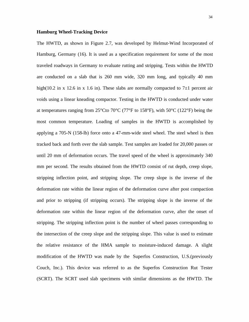
Hamburg Wheel-Tracking Device
The HWTD, as shown in Figure 2.7, was developed by Helmut-Wind Incorporated of
Hamburg, Germany (16). It is used as a specification requirement for some of the most
traveled roadways in Germany to evaluate rutting and stripping. Tests within the HWTD
are conducted on a slab that is 260 mm wide, 320 mm long, and typically 40 mm
high(10.2 in x 12.6 in x 1.6 in). These slabs are normally compacted to 7±1 percent air
voids using a linear kneading compactor. Testing in the HWTD is conducted under water
at temperatures ranging from 25°Cto 70°C (77°F to 158°F), with 50°C (122°F) being the
most common temperature. Loading of samples in the HWTD is accomplished by
applying a 705-N (158-lb) force onto a 47-mm-wide steel wheel. The steel wheel is then
tracked back and forth over the slab sample. Test samples are loaded for 20,000 passes or
until 20 mm of deformation occurs. The travel speed of the wheel is approximately 340
mm per second. The results obtained from the HWTD consist of rut depth, creep slope,
stripping inflection point, and stripping slope. The creep slope is the inverse of the
deformation rate within the linear region of the deformation curve after post compaction
and prior to stripping (if stripping occurs). The stripping slope is the inverse of the
deformation rate within the linear region of the deformation curve, after the onset of
stripping. The stripping inflection point is the number of wheel passes corresponding to
the intersection of the creep slope and the stripping slope. This value is used to estimate
the relative resistance of the HMA sample to moisture-induced damage. A slight
modification of the HWTD was made by the Superfos Construction, U.S.(previously
Couch, Inc.). This device was referred to as the Superfos Construction Rut Tester
(SCRT). The SCRT used slab specimens with similar dimensions as the HWTD. The

35
primary difference between the two was the loading mechanism. The Superfos
Construction Rut Tester. SCRT applied an 82.6-kg (180-lb) vertical load onto a solid
rubber wheel with a diameter of 194 mm and width of 46 mm. This loading configuration
resulted in a contact pressure of approximately 940 kPa (140 psi) and contact area of 8.26
cm2(1.28 in2) which was applied at a speed of approximately 556 mm per second.Test
temperatures ranging from 45°C to 60°C (113°F to 140°F) have been used with the
SCRT. Recent research with the SCRT has used 60°C as the test temperature. An air void
content of 6 percent was generally used for dense-graded HMA samples. Results from the
SCRT are identical to those from the HWTD and include rut depth, creep slope, stripping
slope, and stripping inflection point.
Another slight modification of the HWTD is the Evaluator of Rutting and Stripping
(ERSA) equipment (17). This device was built by the Department of Civil Engineering at
the University of Arkansas. Testing of cylindrical or beam samples in the ERSA can be
conducted in either wet or dry conditions. A 47-mm wide steel wheel is used to load
specimens with 705 N (160lb) for 20,000 cycles or a 20-mm rut depth, whichever occurs
first.

36
Figure 2.7 Model of HWTD
LCPC (French) Wheel Tracker
The Laboratoire Central des Ponts et Chausées (LCPC) wheel tracker [also known as the
French Rutting Tester (FRT)] has been used in France for over 15 years to successfully
prevent rutting in HMA pavements. In recent years, the FRT has been used in the United
States, most notably in the state of Colorado and FHWA's Turner Fairbank Highway
Research Center. The FRT is capable of simultaneously testing two HMA slabs. Slab
dimensions are typically 180 mm wide, 50 mm long, and 20 to 100 mm thick (7.1 in x
19.7 in x 0.8 to 3.9in). Samples are generally compacted with a LCPC compactor with
tires (18). Loading of samples is accomplished by applying a 5000-N (1124-lb) load onto
a 400 x 8 Treb Smooth pneumatic tire inflated to 600 kPa (87 psi). During testing, the
pneumatic tire passes over the center of the sample twice per second. Within France, test
temperatures for FRT testing are generally 60°C (140°F) for surface courses and 50°C
(122°F) for base courses. However, it has been suggested that temperatures lower than

37
60°C (140°F) can be used for colder regions within the United States. Rut depths within
the FRT are defined by deformation expressed as a percentage of the original slab
thickness. Deformation is defined as the average rut depth from a series of 15
measurements. These measurements consist of three measurements taken across the
width of a specimen at five locations along the length of the slab. A "zero" rut depth is
generally defined by loading a sample at ambient temperature for 1,000 cycles.
Figure 2.8 Model of LCPC
Purdue University Laboratory Wheel Tracking Device
As the name states, the PURWheel was developed at PurdueUniversity. PURWheel tests
slab specimens that can either be cut from the roadway or compacted in the laboratory.
Slab specimens are 290 mm wide by 310 mm long (11.4 in x12.2 in). Thickness of slab
samples depends upon the type mixture being tested. For surface course mixes, a sample
thickness of 38 mm (1.5 in) is used while binder and base course mixes are tested at
thickness of 51 mm and 76 mm (2 in and 3 in), respectively.
38
Laboratory samples are compacted using a linear compactor also developed by Purdue
University. This compactor was based upon a similar compactor owned by Koch
Materials in preparing samples for the HWTD. The primary difference being that the
Purdue version can compact larger specimens. Samples are compacted to an air void
content range of 6 to 8 percent. PURWheel was designed to evaluate rutting potential
and/or moisture sensitivity. Test samples can be tested in either dry or wet conditions.
Moisture sensitivity is defined as the ratio of the number of cycles to 12.7 mm of rutting
in a wet condition to the 12.7 mm of rutting in the dry condition. The 12.7-mm rut depth
is used to differentiate between good and bad performing mixes with respect to rutting .
Loading of test samples in PURWheel is conducted utilizing a pneumatic tire. A gross
contact pressure of 620 kPa (90 psi) is applied to the sample. This is accomplished by
applying a 175-kg (385-lb) load onto the wheel that is pressurized to 793 kPa (115 psi). A
loading rate of 332 mm/sec is applied. Testing is conducted to 20,000 wheel passes or
until 20 mm of rutting is developed. PURWheel is very similar to the HWTD. However,
one interesting feature about PURWheel is that it can incorporate wheel wander into
testing. This feature is unique among the LWTs common in the United States.
Model Mobile Load Simulator (MMLS3)
The one-third scale MMLS3 was developed recently in South Africa for testing HMA in
either the laboratory or field. This prototype device is similar to the full-scale Texas
Mobile Load Simulator (TxMLS) but scaled in size and load. The scaled load of 2.1-kN
(472-lb) is approximately one-ninth (the scaling factor squared) of the load on a single

39
tire of an equivalent single axle load carried on dual tires. The MMLS3 can be used for
testing samples in dry or wet conditions. An environmental chamber surrounding the
machine is recommended to control temperature. Temperatures of 50°C and 60°C have
been used for dry tests, and wet tests have been conducted at 30°C. MMLS3 samples are
1.2 m (47 in) in length and 240 mm (9.5 in) in width, with the device applying
approximately 7200 single-wheel loads per hour by means of a 300-mm (12-in) diameter,
80-mm (3-in) wide tire at inflation pressures up to 800 kPa(116 psi) with a typical value
of 690 kPa (100 psi). Wander can be incorporated up to the full sample width of 240 mm.
Performance monitoring during MMLS3 testing includes measuring rut depth from
transverse profiles and determining Seismic Analysis of Surface Waves moduli to
evaluate rutting potential and damage due to cracking or moisture, respectively. Rut
depth criteria for acceptable performance are currently being developed (19). Currently
there is no standard for laboratory specimen fabrication, although research is being
proposed to the Texas Department of Transportation.
2.2.2 Effect of Test Parameters and Mixture Properties on LWT Results
As shown in the previous descriptions on LWTs, all have similar operating principles.
Essentially, a load is tracked back and forth over a HMA test sample. Therefore, the
effect of various test parameters and material constituents should be similar for each.
Following are descriptions of how different test parameters and constituents can affect
LWT results. Within the operating specifications for each of the LWTs, two test
parameters are always specified: air voids and test temperature. This is primarily due to
the fact that these two parameters have the most effect on test results; especially rut
40
depths. As air voids increase, rut depths also increase. Likewise, as test temperature
increases, rut depths also increase.
Air void contents for each of the LWTs are generally specified based upon two concepts.
First, some believe that specimen air void contents should be approximately 7 percent,
since this air void content represents typical as-constructed density. Others believe that
test specimens should be compacted to 4 percent air voids, as actual shear failure of
mixes usually takes place below approximately 3 percent. Another test parameter that can
significantly affect test results is the type and compaction method of test samples. The
two predominant "types" of test specimens are cylinders and beams/slabs. For rutting, the
literature indicates that the two sample types do provide different rut depths; however,
both types generally rank mixes similarly. The primary reason these two types of
specimens do not produce the same rut depths is that they are generally compacted by
different methods. For instance, cylindrical specimens are typically compacted using the
Superpave gyratory compactor while beam samples are generally compacted with a
vibratory or kneading compactor. The method of compaction influences the density (air
void) gradients and aggregate orientation within samples.
Another test parameter that significantly affects test results is the magnitude of loading. A
wide range of loadings are used in the different devices. Although a recent study
indicated that small changes in the magnitude of loading may not affect LWT rut results,
previous research has shown that significant differences in loadings can affect test results.
For rutting, it has been shown that six hours at the test temperature is sufficient. If

41
samples are not preheated sufficiently, low rut depths can be expected. Researchers have
compared identical aggregates and gradations but using different binder grades in LWTs.
When tested at similar temperatures, mixes containing stiffer grades of asphalt binder
will provide lower rut depths. Rutting tends to follow the G*/sin δ of the binder when
tested using the Dynamic Shear Rheometer. Another mixture characteristic that affects
LWT results is nominal maximum aggregate size. For a given aggregate and binder type,
mixes with larger nominal maximum aggregate size gradations tend to provide lower rut
depths.
2.2.3 LWT Results Versus Field Performance
Numerous studies have been conducted to compare results of LWT testing to actual field
performance. Most of these studies have been to relate LWT rut depths to actual field
rutting. In the development of the GLWT, the researchers used four mixes of known
fieldrut performance from Georgia. Three of the four mixes had shown a tendency to rut
in the field. Results of this work showed that the GLWT was capable of ranking mixtures
similar to actual field performance. A similar study conducted in Florida used three mixes
of known field performance. One of these mixes had very good rutting performance, one
was poor, and the third had a moderate field history. Again, results from the GLWT were
able to rank the mixtures similar to the actual field rutting performance. The University
of Wyoming and Wyoming Department of Transportation participated in a study to
evaluate the ability of the GLWT to predict rutting. For this study, 150-mm cores were
obtained from 13 pavements that provided a range of rutting performance. Results
showed that the GLWT correlated well with actual field rutting when project elevation

42
and pavement surface types were considered. The effect of elevation on rut depths was
most likely due to different climates at respective elevation intervals. The Florida
Department of Transportation conducted an investigation with the APA similar to the
GLWT study described previously. Again, three mixes of known field performance were
tested in the APA. Within this study, however, beams and cylinders were both tested.
Results showed that both sample types ranked the mixes similar to the field performance
data. A good correlation was found between the APA and the GLWT test results. The
authors recommended that the average values within the ranges of 7 to 8mm and of 8 to
9mm may be used as a performance limiting criteria at 8000 cycles for beams and
gyratory compacted specimens, respectively. Therefore, the authors concluded that the
APA had the capability to rank mixes according to their rutting potential. Studies by
Prithvi S.Kandhal and Rajib B.Mallick (15) evaluated the APA for HMA mix design.
They found that the APA had a fair correlation (R2 = 0.62) with the repeated shear
constant height test with the shear tester.
The tests on ERSA conducted by the University of Arkansas concluded that the gyratory
compacted specimens exhibited significantly lower rut depths than that of the field
compacted specimens. The specimen configuration (cylindrical versus prismatic beam) is
not a significant factor in performing wheel tracking tests. The study recommended
additional testing to establish and validate the relationship between the performance of
gyratory compacted and field compacted specimens.

43
The Colorado Department of Transportation and the FHWA's Turner FairbankHighway
Research Center participated in a research study to evaluate the FRT and actual field
performance. A total of 33 pavements from throughout Colorado that showed a range of
rutting performance were used. The research indicated that the French rutting
specification (rut depth of less than 10 percent of slab thickness after 30,000 passes) was
too severe for many of the pavements in Colorado. Eleven of 15 sites failed the criteria
despite good pavement performance. However, no sites that passed the French
specification rutted in the field, and the sites that rutted in the field failed the
specification. By reducing the number of passes for low-volume roads and decreasing the
test temperature for pavements located in moderate to high elevations (i.e., colder
climates), the correlation between the FRT results and actual field rutting was greatly
increased.
Another research study by the LCPC compared rut depths from the FRT and field rutting.
Four mixtures were tested in the FRT and placed on a full-scale circular test track in
Nantes, France. Results showed that the FRT can be used as a method of determining
whether a mixture will have good rutting performance. The FHWA conducted a field
pavement study at Turner-Fairbank Highway Research Center using an accelerated
loading facility (ALF). HMA mixtures were produced and placed over an aggregate base
on a linear test section. Three LWTs were used to test mixes placed on the ALF in order
to compare LWT results with rutting accumulated under the ALF. The three LWTs were
the FRT, GLWT, and HWTD. Based upon this study, the results from the LWTs did not
always rank the mixtures similar to the ALF. A joint study by the FHWA and Virginia

44
Transportation Research Council evaluated the ability of three LWTs to predict rutting
performance on mixtures placed at the full-scale pavement study WesTrack. The three
LWTs were the APA, FRT, and HWTD. For this research, 10 test sections from
WesTrack were used. The relationship between LWT and field rutting for all three LWTs
was strong. The HWTD had the highest correlation (90.4%), followed by the APA
(89.9%) and FRT (83.4%). Two important criteria were emphasized. The first criterion is
the selection of an appropriate test temperature at which the pavement will be expected to
perform. The second criterion is the assumption of laboratory compaction simulating
field compaction. The authors quoted studies showing discrepancies between the field
compaction and several laboratory compaction devices.
Three studies by the Texas Department of Transportation utilized the prototype MMLS3
to determine the relative performance of two rehabilitation processes and establish the
predictive capability of this laboratory-scale device. For the first two studies, the MMLS3
tested eight full-scale pavement sections in the field adjacent to sections trafficked with
the TxMLS. Field testing combined with additional laboratory testing indicated that one
of the rehabilitation processes was more susceptible to moisture damage and less resistant
to permanent deformation compared to the second process. This second process was less
resistant to fatigue cracking. In addition, a comparison of pavement response under full-
scale (TxMLS) and scaled (MMLS3) accelerated loading showed good correlation when
actual loading and environmental conditions were considered. An ongoing third study
aims to tie MMLS3 results with actual measured performance of four sections at
WesTrack. A high testing temperature (60°C) was selected based on the critical

45
temperature for permanent deformation during a 5-day trafficking period during which
failure occurred for three of the four sections. Limited laboratory testing using the
HWTD and the APA is also included in this study, but only the rankings from HWTD
results show good correlation with actual performance. Results indicate that the MMLS3
is capable of correctly ranking performance of the four WesTrack sections.
Studies at NCAT (20) recommended the following tests and criteria for the use of LWT
devices for evaluating rutting. The studies considered various factors such as availability
of the equipment, cost, test time, applicability for QC/QA, performance data and ease of
use.
Performance Tests Recommended Criteria Test Temperature
1st choice APA 8mm @ 8000 cycles High temperature for
selected PG grade
2nd choice HWTD 10mm @ 20000 cycles 50oC
3rd choice FRT 10mm @ 30000 cycles 60oC
Based upon review of the laboratory wheel tracking devices and the related literature
detailing the laboratory and field research projects, the following observations are
provided.
*Both cylindrical and beam specimens, depending upon the type of wheel tracking
device, can be used to rank mixtures with respect to rutting.

46
*Results obtained from the wheel tracking devices seem to correlate reasonably well to
actual field performance when the in-service loading and environmental conditions of
that location are considered.
*The wheel tracking devices seem to reasonably differentiate between performance
grades of binders.
*Wheel tracking devices, when properly correlated to a specific site's traffic and
environmental conditions, have the potential to allow the user agency the option of a
pass/fail or "go/no go" criteria. The ability of the wheel tracking devices to adequately
predict the magnitude of the rutting for a particular pavement has not been determined at
this time.

47
CHAPTER 3
MIXTURE INFORMATION
This chapter describes the mixtures used in this study. The mixture description includes
the information about the field specimens and the loose mixtures and their properties
used in this study. Four mixtures were used in this study. They were designated as
Auburn Coarse, Auburn Fine, Charlotte and Kinston mixtures.
3.1 Field Specimens
The field specimens included field cores and field slabs. The location and the total
number of test sites were selected after consultation with NCDOT. Four test sites were
selected in such a way that each test site had a different type of aggregate gradation
(coarse or fine) and a nominal maximum size of aggregate (12.5mm or 9.5mm). The
pavement locations were Auburn NCAT research tracks (Auburn Coarse and Auburn
Fine), Matthews county (Charlotte) and Kinston County (Kinston) in North Carolina. The
aggregates used in these mixtures are from the quarries of North Carolina. These sites
were the pavements that contained SUPERPAVE volumetrically designed mixtures being
used in either new or overlay construction.
Field cores consisted of cylindrical specimens of 150mm diameter with varying heights.
Field cores were taken from all four locations. The cores were catalogued as AC (Auburn
Coarse), AF (Auburn Fine), C (Charlotte) and K (Kinston). The field cores were then
used for shear tests and APA tests. The cores were sawed to a thickness of 50mm and

48
75mm for shear tests and APA tests, respectively. However, the thickness of field cores
for Kinston mixtures was slightly lesser than 75mm. So 70mm thick field cores were
used in APA tests only for the Kinston mixture. The bulk densities of the field cores were
carefully measured using the conventional water displacement method. Table 3.1 shown
below gives the average bulk specific gravity of field cores with their corresponding
range of values.
Table 3.1 Bulk Specific Gravity
Mixture Average BSG Range
Auburn Coarse
Auburn Fine
Charlotte
Kinston
2.362
2.374
2.369
2.268
2.336 to 2.365
2.363 to 2.385
2.347 to 2.415
2.262 to 2.273
For a meaningful comparison of the effect of different compaction methods, the loose
mixtures that were compacted using the laboratory compaction methods were compacted
to the corresponding specific gravities given in Table 3.1.
Field slabs were available only from the Kinston and the Charlotte sites. Field slabs could
not be obtained from the Auburn NCAT research tracks. The slab thickness was 100mm
and 75mm for Charlotte and Kinston mixtures, respectively. The slabs were cut to the
desired dimensions and were used for rut tests using NCSU Wheel Tracking Device.

49
3.2 Loose Mixtures
The mixtures from the test sites were provided as loose mixtures by NCDOT. The loose
mixtures were used to fabricate specimens in laboratory for further evaluation. These
mixtures were heated to the appropriate compaction temperatures for specimen
fabrication. The Superpave Gyratory Compactor and the NCSU WTD rolling wheel
compactor were used for fabricating cylindrical and slab specimens, respectively. The
compaction of slabs using the NCSU WTD roller compactor is discussed in Chapter 5.
Cylindrical specimens, cored from rolling wheel compacted slabs and as well as those
fabricated using the SGC were used for shear tests and APA tests. The slabs were tested
using NCSU WTD for evaluating the rutting characteristics. The loose mixtures were
also used to evaluate the compaction characteristics using the SGC and the GLPA.
The maximum theoretical specific gravity was determined for all the four mixtures. The
mixtures were compacted to the corresponding average bulk densities of the field cores.
In addition to this, in order to rank the performance of individual mixtures, specimens
were compacted to 4 percent air voids using the SGC for shear tests. Table 3.2 gives the
information about the Gmm values and percent air voids for the mixtures compacted using
the SGC and the NCSU WTD rolling wheel compactor.

50
Table 3.2 Target Bulk Densities and Air Voids of Mixtures
Mixture Gmm Target Gmb Percent Air
Auburn Coarse
Auburn Fine
Charlotte
Kinston
2.498
2.477
2.563
2.419
2.362
2.374
2.369
2.268
5.4
4.2
7.6
6.2
3.3 Characteristics of Mixtures
The individual characteristics of mixtures are discussed in the following subsections. The
information about the mixtures as provided by the NCDOT is also presented in here.
3.3.1 Auburn Coarse
This mixture was from the test tracks of NCAT, Auburn. The NCDOT was the contractor
for the North Carolina test sections of this project. This was a surface mix with 12.5mm
nominal maximum size of aggregates with a gradation below the restricted zone. The
coarse gradation of this mixture is shown in Figure 3.1. The source of aggregates was
from Martin Marietta, Jamestown, NC. The effective specific gravity of the aggregates
was 2.709. The grade of asphalt binder used was PG 67-22 with a specific gravity of
1.029. This mixture was designed for a traffic level of 10 to 30 Million ESALs. Gyration
levels used were 8/100/160. The compaction temperature of this mixture was 155oC.
Table 3.3 summarizes the characteristics of the mixture.
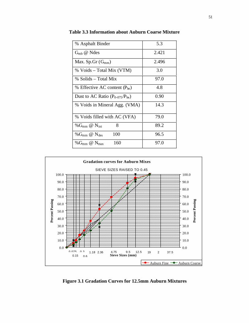
51
Table 3.3 Information about Auburn Coarse Mixture
% Asphalt Binder 5.3
Gmb @ Ndes 2.421
Max. Sp.Gr (Gmm) 2.496
% Voids – Total Mix (VTM) 3.0
% Solids – Total Mix 97.0
% Effective AC content (Pbe) 4.8
Dust to AC Ratio (P0.075/Pbe) 0.90
% Voids in Mineral Agg. (VMA) 14.3
% Voids filled with AC (VFA) 79.0
%Gmm @ Nini 8 89.2
%Gmm @ Ndes 100 96.5
%Gmm @ Nmax 160 97.0
Figure 3.1 Gradation Curves for 12.5mm Auburn Mixtures
Gradation curves for Auburn Mixes
0.0
10.0
20.0
30.0
40.0
50.0
60.0
70.0
80.0
90.0
100.0
Sieve Sizes (mm)
Perc
ent P
assi
ng
0.0
10.0
20.0
30.0
40.0
50.0
60.0
70.0
80.0
90.0
100.0
Perc
ent P
assi
ng
Auburn Fine Auburn Coarse
SIEVE SIZES RAISED TO 0.45
0.075 29.5 1912.54.752.361.180.6
0.30.15
37.5

52
3.3.2 Auburn Fine
This mixture was also from the test tracks of NCAT, Auburn. This mixture was similar to
Auburn Coarse mixture but with a finer gradation. This was a surface mix with 12.5mm
nominal maximum size of aggregates with a gradation above the restricted zone. The fine
gradation of this mixture is shown in Figure 3.1. The source of aggregates was from the
Martin Marietta quarry, Jamestown, NC. The effective specific gravity of the aggregates
was 2.713. The grade of asphalt binder used was PG 67-22 with a specific gravity of
1.029. This mixture was designed for a traffic level of 10 to 30 Million ESALs. Gyration
levels used were 8/100/160. The compaction temperature for this mixture was 155oC.
Table 3.4 summarizes the characteristics of the mixture.
Table 3.4 Information about Auburn Fine Mixture
% Asphalt Binder 5.3
Gmb @ Ndes 2.421
Max. Sp.Gr (Gmm) 2.508
% Voids – Total Mix (VTM) 4.0
% Solids – Total Mix 96.0
% Effective AC content (Pbe) 4.8
Dust to AC Ratio (P0.075/Pbe) 1.21
% Voids in Mineral Agg. (VMA) 14.6
% Voids filled with AC (VFA) 72.0
%Gmm @ Nini 8 88.4
%Gmm @ Ndes 100 96.0
%Gmm @ Nmax 160 97.0

53
3.3.3 Charlotte
This mixture was from the pavement structures constructed in Matthews County of North
Carolina. The Rea Construction Co was the contractor for this project. This was a surface
mix with 9.5mm nominal maximum size of aggregates with a gradation below the
restricted zone. The coarse gradation of this mixture is shown in Figure 3.2. The source
of aggregates was from the Martin Marietta quarry, Matthews, NC. The effective specific
gravity of the aggregates was 2.789. The grade of asphalt binder used was PG 64-22 with
a specific gravity of 1.03. This mixture was designed for a traffic level less than 3 Million
ESALs. Gyration levels used were 7/75/115. The compaction temperature for this
mixture was 149oC. Table 3.5 summarizes the characteristics of the mixture.
Table 3.5 Information about Charlotte Mixture
% Asphalt Binder 5.9
Gmb @ Ndes 2.433
Max. Sp.Gr (Gmm) 2.534
% Voids – Total Mix (VTM) 4.0
% Solids – Total Mix 96.0
% Effective AC content (Pbe) 5.6
Dust to AC Ratio (P0.075/Pbe) 1.14
% Voids in Mineral Agg. (VMA) 17.1
% Voids filled with AC (VFA) 77.2
%Gmm @ Nini 7 86.6
%Gmm @ Ndes 75 96.0
%Gmm @ Nmax 115 97.7

54
Figure 3.2: Gradation Curves for 9.5mm Mixtures (Charlotte and Kinston)
3.3.4 Kinston
This mixture was from the pavement structures constructed in Kinston County of North
Carolina. The contractor of this project was APAC – Carolina (Barrus). This mixture was
a surface mix with 9.5mm nominal maximum size of aggregates with a gradation above
the restricted zone. The fine gradation of this mixture is shown in Figure 3.2. The sources
of aggregates were from the Martin Marietta quarry, Fountain and Clarke, NC. The
natural sand and baghouse fines were from Barrus, Whitfield .The effective specific
gravity of the aggregates was 2.667. The grade of asphalt binder used was PG 64-22 with
a specific gravity of 1.03. This mixture was designed for a traffic level less than 3 Million
ESALs. Gyration levels used were 7/75/115. The compaction temperature for this
mixture was 144oC. Table 3.6 summarizes the characteristics of the mixture.
Gradation Curves for Charlotte and Kinston Mixes
0.0
10.0
20.0
30.0
40.0
50.0
60.0
70.0
80.0
90.0
100.0
Sieve Sizes (mm)
Per
cent
Pas
sing
0.0
10.0
20.0
30.0
40.0
50.0
60.0
70.0
80.0
90.0
100.0
Per
cent
Pas
sing
Charlotte Kinston
SIEVE SIZES RAISED TO 0.45
0.075 29.5 1912.54.752.361.180.6
0.30.15
37.5

55
Table 3.6 Information about Kinston Mixture
% Asphalt Binder 6.1
Gmb @ Ndes 2.334
Max. Sp.Gr (Gmm) 2.431
% Voids – Total Mix (VTM) 4.0
% Solids – Total Mix 96.0
% Effective AC content (Pbe) 5.3
Dust to AC Ratio (P0.075/Pbe) 1.06
% Voids in Mineral Agg. (VMA) 15.8
% Voids filled with AC (VFA) 76
%Gmm @ Nini 7 89.0
%Gmm @ Ndes 75 96.0
%Gmm @ Nmax 115 97.2
The information provided in this chapter was furnished by the NCDOT. The mixtures
were compacted in the laboratory using the SGC to verify the above information. The
densification information and the compaction characteristics evaluated in the laboratory
are discussed in Chapter 4.
56
CHAPTER 4
COMPACTION CHARACTERISTICS OF MIXTURES
The compactability of a mixture can be evaluated by the densification information
generated using the Superpave Gyratory Compactor (SGC) and the Gyratory Load Cell
Plate Assembly (GLPA). This section describes the compaction characteristics of all the
four mixtures included in this study.
4.1 Superpave Gyratory Compactor
The primary device used in Superpave mix design is the Superpave Gyratory Compactor
(SGC). The SGC is used to produce specimens for volumetric analysis, and it also
records data to provide a measure of specimen density throughout the compaction
procedure.
SHRP researchers had several goals in developing a laboratory compaction method (21).
Most importantly, they wanted to realistically compact mix specimens to densities
achieved under actual pavement climate and loading conditions. The compaction device
needed to be capable of accommodating large aggregates. They also wanted the
compactor to be able to measure compactability so that potential tender mix behavior and
similar compaction problems could be identified. A high priority for SHRP researchers
was a device portable enough for use in mixing facility for quality control operations.
Since no existing compactor achieved all these goals, the SGC was developed.

57
The SGC consists of three components:
§ reaction frame, rotating base, and motor
§ loading system, loading ram, and pressure gauge
§ height measuring and recording system
§ mold and base plate
A loading mechanism presses against the reaction frame and applies a load to the loading
ram to produce a 600 kPa compaction pressure on the specimen. A pressure gauge
measures the ram loading to maintain constant pressure during compaction. The SGC
mold has an inside diameter of 150mm and a base plate in the bottom of the mold
provides confinement during compaction. The SGC base rotates at a constant 30
gyrations per minute during compaction with the mold positioned at a compaction angle
of 1.25 degrees.
Specimen height measurement is an important function of the SGC. Specimen density
can be estimated during compaction by knowing the mass of material placed in the mold,
the inside diameter of the mold, and the specimen height. Height is measured by
recording the position of the ram throughout the test. Using these measurements, a
specimen’s compaction characteristics are developed.

58
4.2 SGC Compaction of Mixtures
The loose mixtures were compacted in the laboratory not only to evaluate the compaction
characteristics of the mixtures but also to establish the parameters such as “correction
factors” for fabricating specimens at the average bulk densities of the respective field
cores. The compacted specimens were used for shear tests and APA tests. The loose
mixtures were heated and mixed thoroughly. The amount of mixture was sampled out for
compaction of mixture specimens (approximately 4800g for one specimen). These were
field mixtures and therefore they were aged before compacting. The mixtures were
heated at their corresponding compaction temperatures. The mixtures were placed in the
mold and compacted using the SGC. Compaction proceeded until Nmax had reached.
Specimen height was continually monitored during compaction and a height
measurement was recorded after each gyration. Table 4.1 gives the compaction
temperature and desired levels of gyrations for each mixture.
Table 4.1 : Levels of Gyrations and Compaction Temperatures
Mixture NMSA, mm Gradation Temperature Nini Ndes Nmax
Auburn Coarse
Auburn Fine
Charlotte
Kinston
12.5
12.5
9.5
9.5
Coarse
Fine
Coarse
Fine
155 oC
155 oC
149 oC
144 oC
8
8
7
7
100
100
75
75
160
160
115
115
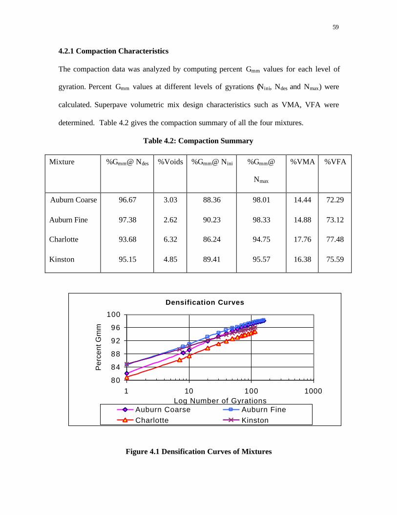
59
4.2.1 Compaction Characteristics
The compaction data was analyzed by computing percent Gmm values for each level of
gyration. Percent Gmm values at different levels of gyrations (Nini, Ndes and Nmax) were
calculated. Superpave volumetric mix design characteristics such as VMA, VFA were
determined. Table 4.2 gives the compaction summary of all the four mixtures.
Table 4.2: Compaction Summary
Mixture %Gmm@ Ndes %Voids %Gmm@ Nini %Gmm@
Nmax
%VMA %VFA
Auburn Coarse
Auburn Fine
Charlotte
Kinston
96.67
97.38
93.68
95.15
3.03
2.62
6.32
4.85
88.36
90.23
86.24
89.41
98.01
98.33
94.75
95.57
14.44
14.88
17.76
16.38
72.29
73.12
77.48
75.59
Figure 4.1 Densification Curves of Mixtures
Densification Curves
80
84
88
92
96
100
1 10 100 1000Log Number of Gyrations
Per
cent
Gm
m
Auburn Coarse Auburn FineCharlotte Kinston

60
Figure 4.1 shows the densification characteristics of each mixture. Percent Gmm values
were plotted against the corresponding gyrations on a logarithmic scale. A logarithmic
regression for percent Gmm was performed for each curve with number of gyration (N) as
predictor variable. Table 4.3 shows the regression equation for each mixture with the
corresponding R2 values.
Table 4.3: Regression Equation of Compaction Curves
Mixture Equation R2
Auburn Coarse
Auburn Fine
Charlotte
Kinston
%Gmm = 3.2132 ln(N) + 82.104
%Gmm = 2.7095 ln(N) + 84.899
%Gmm = 2.9669 ln(N) + 80.816
%Gmm = 2.3514 ln(N) + 85.429
0.9966
0.9963
0.9985
0.9986
It was found from the densification curves and compaction summary that none of the
mixtures had the recommended 4 percent air voids at Ndes. The air voids level was closer
to 4 percent criterion for the Kinston mixture. The percent air values at Ndes were only
around 2 percent for the Auburn mixtures. The percent air at Ndes was above 6 percent for
the Charlotte mixtures. The compaction characteristics of the Auburn coarse and fine
mixtures were almost similar. They seemed to be easier to compact than other mixtures.
The Charlotte mixture was the most difficult mixture to compact among all the mixtures.

61
A noteworthy characteristic in the evaluation of Superpave mixtures is the slope of the
compaction curve (kSGC), percent Gmm versus log N(22). The compaction slope is an
indication of an aggregate structure’s resistance to compaction. Since the SGC operates
as a gyratory shear compactor, the slope of the compaction curve might be considered
related to the shear resistance of the aggregate structure. The slope of the compaction
curve is calculated by considering the percent Gmm values between the gyrations 10 to
100. The values of kSGC are given in Table 4.4.
Table 4.4 : Compaction Slope of Mixtures
Mixture %Gmm @ N=10 %Gmm @ N=100 kSGC
Auburn Coarse
Auburn Fine
Charlotte
Kinston
89.22
90.97
87.32
90.79
96.97
97.38
94.16
96.11
7.75
6.41
6.84
5.32
The Auburn Coarse mixture had the highest compaction slope whereas Kinston mixture
had the lowest compaction slope. A mixture with higher compaction slope is expected to
offer more resistance to compaction. The slopes of the Auburn Fine mixture and the
Charlotte mixture are closer to each other. It appears that the Auburn Coarse mixture had
the highest shear resistance and Kinston mixture had the lowest shear resistance among
all the mixtures.

62
Another characteristic in the evaluation of Superpave mixture is the Gyration Ratio (GR)
(23). The Gyration Ratio is the ratio of the number of gyrations by the SGC to achieve 95
percent Gmm to the number of gyrations to achieve 98 percent Gmm. This ratio actually
gives an indication of the change of stiffness of the mixture between 5 and 2 percent air
voids. Table 4.5 shows the values of GR for each mixture.
Table 4.5: Gyration Ratio of Mixtures
Mixture N for 95%Gmm N for 98%Gmm GR
Auburn Coarse
Auburn Fine
Charlotte
Kinston
50
37
119*
55
160
132
328*
210*
3.20
3.56
2.76
3.82
* Extrapolated from the regression equation given in Table
The Charlotte mixture did not reach 95% Gmm at Nmax. So it was assumed that the mixture
would reach the above percent Gmm values at the extrapolated number of gyrations. The
same was applied for Kinston mixture. It should be borne in mind that the extrapolated N
values are based only on the logarithmic regression fit of the densification information
obtained from the SGC. Based on the number of gyrations that a mixture took to reach
the desired compaction level (95%Gmm or 98%Gmm), it was found that the Auburn
mixtures were easier to compact and the Charlotte mixture was the difficult mixture to
compact, followed by the Kinston mixture.

63
4.2.2 Compaction using Pine SGC
For computing the energy indices using the SGC and the GLPA, the compaction of the
mixtures was done using Pine SGC and GLPA. In addition to the computation of energy
indices, the percent Gmm values at initial, design and maximum levels of gyrations are
calculated. Table 4.6 gives the values of percent Gmm at different levels of gyrations.
Table 4.6 Compaction Summary (Pine SGC)
Mixture %Gmm@ Ndes %Voids %Gmm@ Nini %Gmm@ Nmax
Auburn Coarse
Auburn Fine
Charlotte
Kinston
97.06
96.92
93.68
95.15
2.94
3.08
6.32
4.85
88.20
89.36
87.71
87.34
98.16
97.92
94.60
96.30
It should be noted that the compaction summary of the mixtures provided by the NCDOT
does not agree with the compaction results obtained at NCSU. The compaction
parameters of the mixtures measured using the Troxler SGC and the Pine SGC agreed
with each other. Moreover through out this study, the specimens compacted at target air
voids were found to be the same when the compaction parameters measured at NCSU
were used for calculations. So it can be said that the compaction summary given in Table
4.2 is found to be accurate though it does not conform to the information provided by the
NCDOT.

64
4.3 Gyratory Load Cell Plate Assembly
Measurement of mechanical properties to evaluate mixture performance is not a new
concept. One of the most important criticisms of the Superpave volumetric design
procedure is the lack of a direct measure of mechanical properties of asphalt mixtures and
the reliance on the control of densification characteristics. Gyratory Load Plate Assembly
(GLPA) was developed to apply a two dimensional distribution of shear resistance as
measured on the top of the specimen (24).
The plate includes 3 load cells equally spaced on the perimeter of a double-plate
assembly, which can be inserted on the sample of the HMA in a typical gyratory mold.
The load cells allow measuring the variation in distribution of force on top of the sample
during the gyrations such that the position of the resultant force on top of the sample
during the gyrations such that the position of the resultant force from the gyratory
compactor can be determined in real time. The two dimensional distribution of the
eccentricity of the resultant load can be used to calculate the effective moment required to
overcome the shear resistance of mixtures and tilt the mold to conform to the 1.25 degree
angle.
It is believed that this effective moment is a direct measure of the resistance of asphalt
mixtures to distortion and to densification. Because the densification is being measured
by the compactor, the measured moment can be used to separate the energy spent in
densification from the energy spent in distortion. The distortion energy is believed to be
related to the resistance of the mixture to rutting under traffic.

65
4.3.1 Description of GLPA
The main components of the GLPA are three 9kN load cells, two hardened steel plates
that can fit into the compaction mold and a computer for data acquisition from both
GLPA and SGC device. The load cells are placed on the upper plate of the assembly at a
common radial distance, 120o apart. Each load cell is attached by three screws so that the
load pins of each load cell have a small contact point on the lower plate which is in
contact with the hot mixture during the compaction. The load cells are designed for high
temperature applications and were calibrated by the manufacturer at the level of typical
compaction temperatures. Three connecting pins hold the steel plates together and
maintain the alignment of the plates. The upper plate is slightly smaller in radius than the
lower plate to allow for tilting of the plate assembly in the mold. The plate assembly can
be easily placed on top of the mixture sample within the mold using a suction cup. The
load cells are simply connected to the data acquisition system by a cable that extends
from the top plate to the gyratory ram. During the compaction process, readings are taken
at a rate of 50 readings per gyration from each load cell using signal conditioning and
acquisition hardware controlled by the graphical programming language LabVIEW.
Deflection readings can also be recorded in real time by the system through the serial
communication port of the SGC device. A schematic diagram is given in Figure 4.2
Based on the readings from the load cells, the two components of eccentricity of the total
load relative to the center of the plate (ex and ey) can be calculated for each of the 50
points collected during each gyration. The calculations are done using general moment
equilibrium equations along two perpendicular axes passing through the center of one of
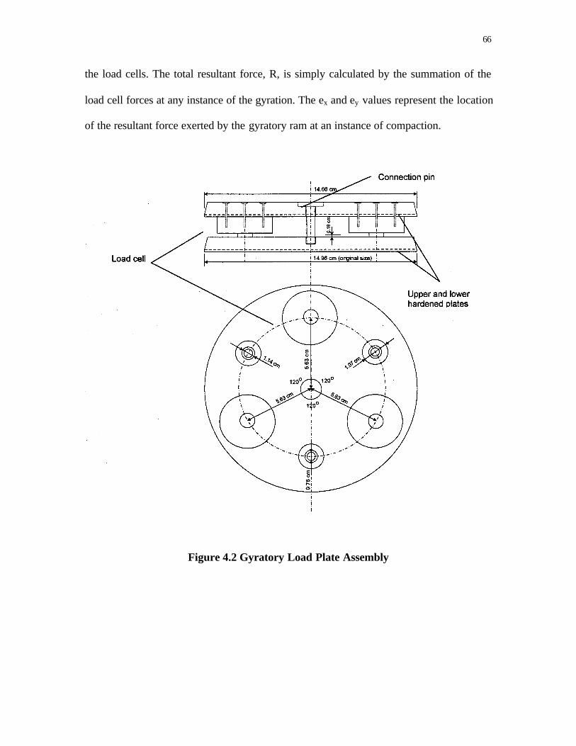
66
the load cells. The total resultant force, R, is simply calculated by the summation of the
load cell forces at any instance of the gyration. The ex and ey values represent the location
of the resultant force exerted by the gyratory ram at an instance of compaction.
Figure 4.2 Gyratory Load Plate Assembly

67
4.4 Energy Indices
The performance of HMA can be divided into two parts, performance during construction
and performance under traffic loading (25). In both parts, there are two basic
characteristics that control performance: (a) resistance to densification, or volume
change, and (b) resistance to distortion, also called shear resistance or stability. During
the construction part, less resistance to densification and to distortion are considered
favorable because it implies less compaction energy is required to achieve required
density. In the second part, performance under traffic, more resistance to densification
and to distortion is considered favorable because it implies that mixture can tolerate more
traffic before reaching a certain level of rutting. Although densification and distortion are
not necessarily independent properties, they need to be measured independently because
distortion could be measured at a constant volume (no densification).
The researchers of the University of Wisconsin Madison developed energy indices as
measures of densification and distortion under construction and under traffic. The areas
under the densification curve between selected reference points are related to the actual
field construction and in-service conditions as indicators of mixture suitability for
construction and performance under traffic. The energy indices are calculated by
integrating the area under the densification curve between any two given points.
The Compaction Densification Index (CDI) and Compaction Force Index (CFI) are used
to evaluate the performance of mixtures during construction. CDI is measured by
integration of the area under the densification curve measured by the SGC between the

68
first gyration and the 92% Gmm. The 92% Gmm is assumed to be the target density at the
end of construction. The CFI is the integration of the area under the resistive work curve
measured with the GLPA between the same reference points. This effort is the work
applied by the pavers/rollers to compact the mix to the required density during
construction. The initial in-place density behind the paver is not constant and depends on
the characteristics of the mix. The initial density after the rolling operation (at the end the
construction) is well defined at a certain air voids level. Many specifications require that
the pavement be compacted to approximately 92 percent of Gmm for acceptance. The
energy that the contractor must expend in compacting the mix from its initial density to
the required density at the end of rolling is estimated by these indices. Mixes that require
lower compaction energy are desirable.
To measure the mixture resistance to traffic, the Traffic Densification Index (TDI) and
Traffic Force Index (TFI) are used. TDI and TFI are estimated by integration of the area
under the densification and resistive work curves between 92% Gmm and 98% Gmm as
shown in Figure 4.3. These indices represent the total effort required to compact the
mixture to a terminal density of 98 percent Gmm. The 98 percent Gmm is considered the
critical density condition at which the mix is within the plastic failure zone. Mixtures
with higher traffic indices are more desirable because they are expected to require more
traffic to densify at that point. It should be noted that there exists a strong correlation
within the two construction indices (CDI & CFI) and the two traffic indices (TDI & TFI).
The Densification indices (CDI & TDI) are measured using the SGC and the Force
indices (CFI & TFI) are measured using the GLPA.

69
Figure 4.3 Energy Indices (CDI, CFI,TDI,TFI)

70
The resultant force, which is measured by the load cells, can be used to explain the
behavior of the mixtures. The average values of the amplitude of the load carried by three
load cells are shown in Figure 4.4. The plot shows the maximum and minimum load
carried by the load cells for each of the mixtures. The maximum load cell amplitude of
the mixtures is given in Table 4.7.
Table 4.7 Maximum Amplitude carried by the Load Cells
Mixture Max. Amplitude (kN)
Auburn Coarse
Auburn Fine
Charlotte
Kinston
7.64
7.33
7.38
7.64
Figure 4.4 Maximum and Minimum Load Cell Amplitudes of Mixtures
The load cell amplitudes of all the mixtures were in a narrow range. Moreover, it was
observed that the load cell force had a minor change with increasing gyrations. This
Max & Min Load Cell Force
02468
10
0 50 100 150Gyrations
Load
Cel
l For
ce
Auburn Coarse Auburn FineCharlotte Kinston
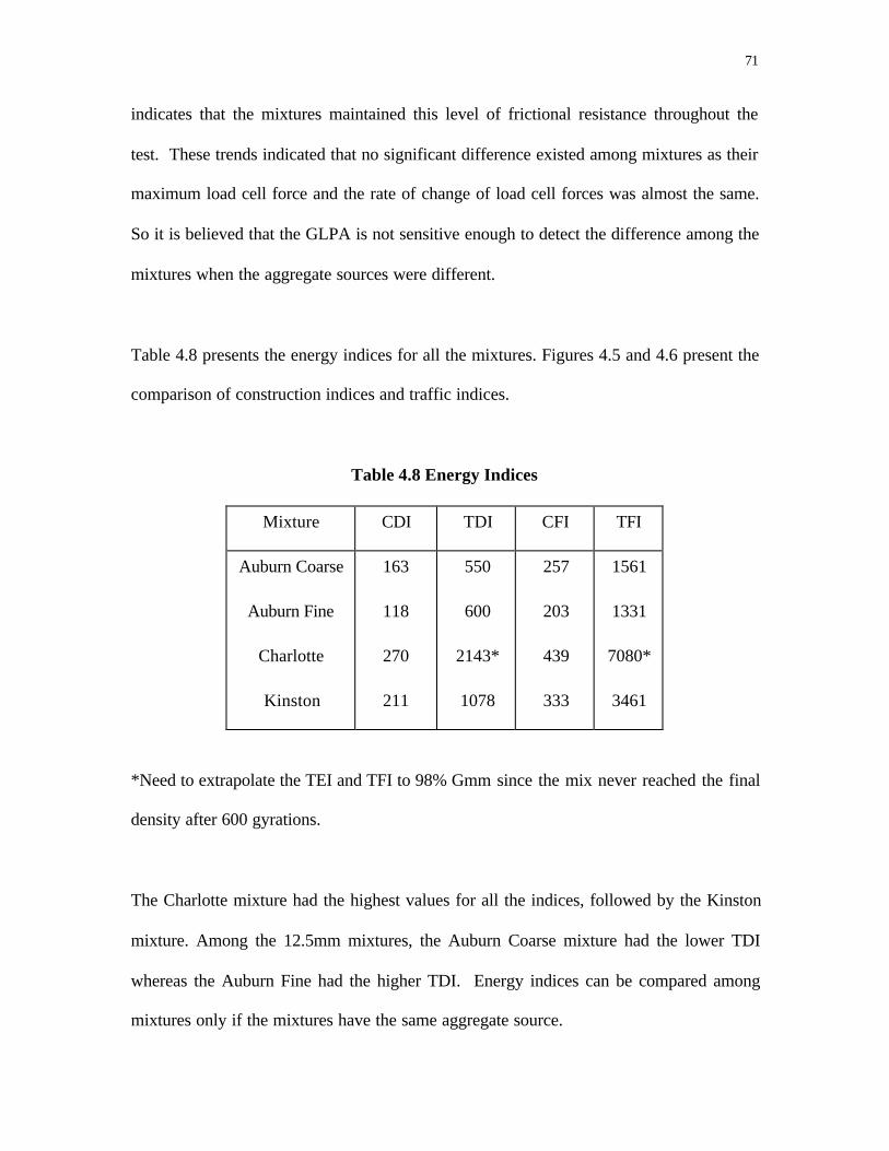
71
indicates that the mixtures maintained this level of frictional resistance throughout the
test. These trends indicated that no significant difference existed among mixtures as their
maximum load cell force and the rate of change of load cell forces was almost the same.
So it is believed that the GLPA is not sensitive enough to detect the difference among the
mixtures when the aggregate sources were different.
Table 4.8 presents the energy indices for all the mixtures. Figures 4.5 and 4.6 present the
comparison of construction indices and traffic indices.
Table 4.8 Energy Indices
Mixture CDI TDI CFI TFI
Auburn Coarse
Auburn Fine
Charlotte
Kinston
163
118
270
211
550
600
2143*
1078
257
203
439
333
1561
1331
7080*
3461
*Need to extrapolate the TEI and TFI to 98% Gmm since the mix never reached the final
density after 600 gyrations.
The Charlotte mixture had the highest values for all the indices, followed by the Kinston
mixture. Among the 12.5mm mixtures, the Auburn Coarse mixture had the lower TDI
whereas the Auburn Fine had the higher TDI. Energy indices can be compared among
mixtures only if the mixtures have the same aggregate source.

72
Figure 4.5: Construction Indices
Figure 4.6: Traffic Indices
Construction Indices
163257
118203270
439
211333
0
200
400
600
CEI CFI
Auburn Coarse Auburn Fine Charlotte Kinston
Traffic Indices
5501561
6001331
2143
7080
1078
3461
0
2000
4000
6000
8000
TEI TFIAuburn Coarse Auburn Fine Charlotte Kinston

73
A review of the construction indices suggested that the Auburn Fine mixture would
require less energy for compaction than other mixtures. The Auburn Fine mixture was the
most desirable for compaction during construction, followed by the Auburn Coarse and
the Kinston. The Charlotte mixture would require greater energy than the other mixtures.
Lower construction indices and higher traffic indices are desirable for selecting an
optimum mixture for constructability and resistance to traffic. This trend is not seen in
the Kinston and the Charlotte mixtures, as the sources of the aggregates used in the
mixtures were not the same. However, the Auburn mixtures seemed to be comparable, as
their sources of the aggregates remained the same. The Auburn Fine mixture had the
lower CDI and higher TDI when compared to the Auburn Coarse mixture, which further
indicated that the Auburn Fine mixture would perform better than the Auburn Coarse
mixture.
Higher traffic indices indicate longer rut life as it is expected that the mixture would
require more traffic to reach their terminal density (11). Before comparing these indices
to evaluate the performance of the mixture under traffic, the explanation given in the
succeeding paragraphs should be taken into account.
Auburn mixtures were compacted to 160 gyrations whereas the Charlotte and Kinston
mixtures were compacted to 600 gyrations. As per the definition, the construction indices
are the integration of the area under the densification curve between the first gyration and

74
the 92% Gmm. On the other hand, the traffic indices are the integration of the area under
the densification and resistive work curves between 92%Gmm and 98% Gmm.
Figure 4.7 shows the densification curves for the mixtures.
Figure 4.7 Densification Curves of Mixtures
It can be noted from the densification curves shown in Figure 4.7 that only the Auburn
mixtures reached their 98 percent of maximum density in 160 gyrations. Charlotte and
the Kinston mixtures did not reach their 98 percent of maximum density in Nmax (115
gyrations). So in order to make the mixtures reach the 98 percent of maximum density,
these mixtures had been compacted to 600 gyrations. The Kinston mixture reached its 98
%Gmm around 270 gyrations. The Charlotte mixture did not reach its 98 % Gmm even
after 600 gyrations. So the traffic indices were calculated by extrapolation. The reason for
very high values of traffic indices for the Charlotte and the Kinston mixtures is that these
mixtures took more number of gyrations than the Auburn mixtures.
Densification Curves
80
84
88
92
96
100
1 10 100 1000Gyrations
Per
cent
Gm
m
Auburn Coarse Auburn Fine
Charlotte Kinston

75
Brian J.Coree and Kera VanDerHorst (10) argue that the resulting compaction curve
cannot be considered to be fully representative of the compaction history of an in-service
mixture. The temperature of the mixture is typically in the range of 80oC to 200oC during
construction. The greater part of compaction is achieved while the asphalt mixture is in
excess of 115oC. The mixture never reaches such a high temperature in-service. Under
operating conditions under traffic, the mixture temperature may reach in the range
indicated by the PG X-Y grade of the binder. In the laboratory, mixtures are compacted at
an equi-viscous temperature through out the compaction process.
Moreover, the lateral plastic flow developed in a pavement rutting is totally prevented
during the compaction, as the walls of the mold are well confined and rigid. Thus the
laboratory compaction is reasonable representation of the construction compaction
conditions, but not of in-service conditions.
So these concerns about the traffic indices limit the evaluation of mixtures only to the
constructability of the mixtures. In this study, the rutting characteristics of the mixtures
are not inferred from the traffic indices. The rutting characteristics of the mixtures are
discussed in Chapter 5.

76
CHAPTER 5
PERFORMANCE EVALUATION OF MIXTURES
The effect of different compaction methods on the performance of the mixtures was
evaluated using the Simple Shear Tester, Asphalt Pavement Analyzer (APA), NCSU
Wheel Tracking Device and GLPA. In addition, the results of the different test systems
helped in evaluating accelerated test devices like the APA and the NCSU WTD in
comparison with fundamental tests like Simple Shear tests.
5.1 Performance Evaluation using the Simple Shear Tester
Shear tests were performed in accordance with AASHTO TP7 Procedures E and F (26).
The tests included Frequency Sweep test at Constant Height (FSCH) and Repeated Shear
test at Constant Height (RSCH). These tests were conducted on the field cores (FC),
Superpave gyratory compacted specimens (SGC), and rolling wheel compacted
specimens (RWC). Field mixtures were compacted to the corresponding field densities
and the tests were performed at the bulk densities of the field cores. The test results were
then used to perform an analysis of a representative pavement structure to investigate the
effect on the predicted field performance.
5.1.1 Specimen Preparation
The specimens prepared for FSCH and RSCH tests were 150mm (6-in.) in diameter. The
specimens were sawed to a thickness of 50 mm (2-in.). The specific gravities of the
specimens were measured. The specimens were then glued between the loading platens

77
using the ‘DEVCON’ 5 minute plastic putty and were allowed to cure for several hours
before testing.
5.1.2 Selection of Test Temperature for FSCH and RSCH
In the abridged fatigue analysis (SHRP A-003A) procedure, the pavement temperature is
assumed to be 20oC through out the year. The resistance of a mix to fatigue cracking is
calculated based on the mix properties evaluated using FSCH at 20oC.
The seven-day average high pavement temperature at 50-mm depth from pavement
surface at 98% reliability was estimated using SHRPBIND version 2.0 software for three
different locations - Auburn (AL), Charlotte (NC) and Kinston (NC). RSCH tests were
conducted on field cores at these temperatures. The testing temperatures for each mixture
are summarized in Table 5.1.
Table 5.1 Testing Temperatures
Mix FSCH RSCH
Auburn – Coarse
Auburn Fine
Charlotte
Kinston
20
20
20
20
54.1
54.1
51.9
50.8
5.1.3 Frequency Sweep Test at Constant Height
This test is performed to measure linear visco-elastic properties of asphalt concrete for
rutting and fatigue cracking analysis. This test uses a dynamic type of loading and is a
strain controlled test with the maximum shear strain limited to ± 0.005 percent
78
(maximum peak to peak of 0.0001 mm/mm). This test is conducted at a constant height
requiring the vertical actuator to be controlled by the vertical LVDT. The specimen is
preconditioned by applying a sinusoidal horizontal shear strain with amplitude of
approximately 0.0001 mm/mm at a frequency of 10 Hz for 100 cycles. After
preconditioning the specimen, a series of 10 tests are conducted in descending order of
frequency. The following order of frequencies is used: 10, 5, 2, 1, 0.5, 0.2, 0.1, 0.05, 0.02
and 0.01 Hz. A specific number of cycles between 4 and 50 are applied. During the test,
axial and shear loads and deformations are measured and recorded.
This test was conducted according to AASHTO TP-7 Procedure E. Four mixtures viz,
Auburn Coarse, Auburn Fine, Charlotte and Kinston were tested at a temperature of
20oC. Dynamic Shear Modulus and Phase angle was measured at each frequency for each
mixture. The ratio of the stress response of the test specimen to the applied shear strain is
used to compute a complex modulus for a given frequency. The delay in the response of
the material is measured as phase angle. From the test results, the following graphs are
generated to evaluate the mix properties:
• Dynamic Shear Modulus (|G*|) vs frequency (on log scale)
• Phase angle vs frequency (on log scale)
5.1.3.1 Analysis of FSCH Test Results
Figures 5.1 to 5.3 show the results of frequency sweep tests for all the mixtures. The
figures show the dynamic shear modulus (G*) as a function of frequency at 20oC. The
figures are plotted for the mixtures according to their method of compaction. Tables 5.2
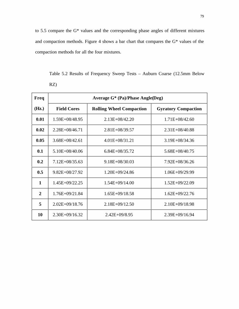
79
to 5.5 compare the G* values and the corresponding phase angles of different mixtures
and compaction methods. Figure 4 shows a bar chart that compares the G* values of the
compaction methods for all the four mixtures.
Table 5.2 Results of Frequency Sweep Tests – Auburn Coarse (12.5mm Below
RZ)
Average G* (Pa)/Phase Angle(Deg)Freq
(Hz.) Field Cores Rolling Wheel Compaction Gyratory Compaction
0.01 1.59E+08/48.95 2.13E+08/42.20 1.71E+08/42.60
0.02 2.28E+08/46.71 2.81E+08/39.57 2.31E+08/40.88
0.05 3.68E+08/42.61 4.01E+08/31.21 3.19E+08/34.36
0.1 5.10E+08/40.06 6.84E+08/35.72 5.68E+08/40.75
0.2 7.12E+08/35.63 9.18E+08/30.03 7.92E+08/36.26
0.5 9.82E+08/27.92 1.20E+09/24.86 1.06E+09/29.99
1 1.45E+09/22.25 1.54E+09/14.00 1.52E+09/22.09
2 1.76E+09/21.84 1.65E+09/18.58 1.62E+09/22.76
5 2.02E+09/18.76 2.18E+09/12.50 2.10E+09/18.98
10 2.30E+09/16.32 2.42E+09/8.95 2.39E+09/16.94

80
Table 5.3 Results of Frequency Sweep Tests – Auburn Fine (12.5mm Above RZ)
Average G* (Pa)/Phase Angle(Deg)Freq
(Hz.) Field Cores Rolling Wheel Compaction Gyratory Compaction
0.01 1.55E+08/43.85 3.16E+08/34.73 1.69E+08/46.14
0.02 1.99E+08/41.98 4.08E+08/31.59 2.32E+08/44.85
0.05 2.81E+08/36.81 5.59E+08/26.25 3.59E+08/40.41
0.1 4.32E+08/40.84 7.91E+08/27.79 5.98E+08/42.09
0.2 5.89E+08/37.42 1.01E+09/23.98 9.18E+08/36.35
0.5 8.07E+08/30.30 1.23E+09/19.15 1.20E+09/27.02
1 1.13E+09/27.12 1.61E+09/14.38 2.04E+09/19.14
2 1.25E+09/23.62 1.86E+09/16.39 1.89E+09/21.46
5 1.69E+09/21.56 2.19E+09/11.74 2.66E+09/18.14
10 1.96E+09/18.73 2.40E+09/10.85 2.98E+09/13.27
Table 5.4 Results of Frequency Sweep Tests – Charlotte (9.5mm Below RZ)
Average G* (Pa)/Phase Angle(Deg)Freq
(Hz.) Field Cores Rolling Wheel Compaction Gyratory Compaction
0.01 3.78E+07/46.27 7.13E+07/46.43 8.73E+07/41.46
0.02 4.86E+07/48.22 9.44E+07/44.83 1.11E+08/40.98
0.05 7.04E+07/48.12 1.36E+08/42.52 1.53E+08/36.54
0.1 1.04E+08/49.12 2.21E+08/43.53 2.58E+08/43.67
0.2 1.44E+08/48.14 2.98E+08/41.79 3.44E+08/42.00
0.5 2.31E+08/46.12 4.46E+08/37.90 5.09E+08/37.55
1 3.30E+08/45.25 5.97E+08/35.10 6.80E+08/34.28
2 4.66E+08/41.50 7.63E+08/29.94 8.67E+08/30.80
5 7.07E+08/37.36 1.07E+09/28.31 1.18E+09/27.38
10 9.45E+08/33.34 1.31E+09/25.03 1.44E+09/25.41

81
Table 5.5 Results of Frequency Sweep Tests – Kinston (9.5mm Above RZ)
Average G* (Pa)/Phase Angle(Deg)Freq
(Hz.) Field Cores Rolling Wheel Compaction Gyratory Compaction
0.01 2.01E+07/51.32 6.57E+07/47.66 8.50E+07/43.24
0.02 2.81E+07/54.04 8.99E+07/45.80 1.12E+08/42.64
0.05 4.92E+07/55.93 1.34E+08/43.19 1.61E+08/39.87
0.1 5.92E+07/52.86 2.00E+08/43.96 2.33E+08/41.54
0.2 9.31E+07/55.77 2.71E+08/41.85 3.11E+08/39.60
0.5 1.49E+08/50.72 4.05E+08/36.16 4.56E+08/33.02
1 2.18E+08/50.09 5.45E+08/35.01 6.00E+08/32.54
2 3.16E+0846.46 7.13E+08/31.38 7.60E+08/29.01
5 4.88E+08/41.67 9.74E+08/28.31 1.01E+09/25.75
10 6.63E+08/37.51 1.21E+09/24.76 1.22E+09/23.07
Figure 5.1 Frequency Sweep Test Results of Field Cores
FSCH Test: Field Cores (FC)
0.00E+005.00E+081.00E+091.50E+092.00E+092.50E+093.00E+093.50E+09
0.01 0.1 1 10
Frequency, Hz
G*,
Pa
Auburn Coarse Auburn Fine Charlotte Kinston

82
Figure 5.2 Frequency Sweep Test Results of RWC Specimens
Figure 5.3 Frequency Sweep Test Results of SGC Specimens
FSCH Test: Rolling Wheel Compaction (RWC)
0.0E+00
5.0E+08
1.0E+09
1.5E+09
2.0E+09
2.5E+09
3.0E+09
3.5E+09
0.01 0.1 1 10Frequency
G*,
Pa
Auburn Coarse Auburn Fine Charlotte Kinston
FSCH Test:Gyratory Compaction (SGC)
0.0E+005.0E+081.0E+091.5E+092.0E+092.5E+093.0E+093.5E+09
0.01 0.1 1 10
Frequency, Hz
G*,
Pa
Auburn Coarse Auburn Fine Charlotte Kinston

83
The test results show that the G* values of the Auburn mixtures were almost twice that of
the Charlotte and the Kinston mixtures. Similarly, the phase angles of the Auburn
mixtures were half that of the other mixtures. In other words, the 12.5mm mixtures were
stiffer than the 9.5mm mixtures. The same behavior was noticed for all the three methods
of compaction. The Auburn Coarse mixture was the stiffest among the field cores and the
RWC specimens, whereas the Auburn Fine mixture was the stiffest among the gyratory
compacted specimens. The Kinston mixture had the lowest stiffness among all the
mixtures and compaction methods.
For the Auburn Coarse mixture, the rolling wheel compaction provided the highest G*
values and lowest phase angle than the other compaction methods. But there seemed to
be very little difference between the G* values of the SGC mixtures and RWC mixtures.
For the Auburn Fine mixtures, the gyratory compaction provided the highest G* values
than the field cores and the rolling wheel compaction. The same trend was reflected in the
Charlotte and the Kinston mixtures.
Figure 5.4 Comparison of G* @ 10 Hz
FSCH Test: G*@10Hz
0.00E+00
1.00E+09
2.00E+09
3.00E+09
AuburnCoarse
AuburnFine
Charlotte Kinston
G*,
Pa
FC RWC SGC

84
There was no definite trend in the phase angles of the mixtures. The phase angles of field
cores were higher than the phase angles of RWC and SGC specimens for all of the
mixtures. For the Charlotte and the Kinston mixtures, the phase angles of RWC and SGC
specimens were almost equal; but for the Auburn mixtures, the phase angles of RWC
specimens were lower than that of SGC specimens. The phase angles play a significant
role in determining the viscous and elastic components of the mixture behavior and in
estimating the fatigue life of the mixtures.
In general, it can be stated that the gyratory compaction provided the mixtures with
higher stiffness than the field cores and the RWC mixtures. The field cores had the lowest
stiffness among the three methods of compaction. The RWC mixtures have stiffness
values in between the field cores and SGC mixtures. This indicates that laboratory
compaction methods provide specimens that over estimate the stiffness properties of the
field cores.
The results discussed above were the shear tests performed on four different types of
mixtures at the corresponding densities of their respective field cores. The tests results
furnished in Tables 5.2 to 5.5 can be used to compare the effect of different compaction
methods on different mixtures.
One of the objectives of this study was to evaluate how changes in asphalt content and
aggregate gradation affect mixture compaction and predicted performance. The mixtures
used in this study had two different asphalt grades (PG 67 and PG 64), nominal
maximum size of aggregates (12.5 and 9.5mm), aggregate gradations (above and below

85
the restricted zone) and different sources of aggregates. In order to evaluate the effect of
these differences, the bulk density of all the mixtures should be the same for their
performance evaluation. The shear tests were conducted on specimens compacted at four-
percent air voids using the Superpave Gyratory compactor. Table 5.6 and Figure 5.5
show the results of FSCH tests performed on mixtures compacted at four- percent air
voids.
Table 5.6 Results of Frequency Sweep Tests – SGC Specimens at 4% Air Voids
Average G* (Pa)/Phase Angle(Deg)Freq
(Hz.) Auburn Coarse Auburn Fine Charlotte Kinston
0.01 4.03E+08/38.10 4.18E+08/35.73 2.61E+08/35.39 1.15E+08/44.57
0.02 5.23E+08/35.96 5.37E+08/33.31 3.32+08/34.31 1.53E+08/43.53
0.05 7.44E+08/31.06 7.33E+08/27.71 4.56E+08/30.48 2.27E+08/40.48
0.1 1.12E+09/32.30 1.08E+09/29.27 6.30E+08/32.85 3.17E+08/40.88
0.2 1.46E+09/28.96 1.41E+09/25.60 8.16E+08/29.87 4.27E+08/38.31
0.5 1.89E+09/25.68 1.68E+09/21.32 1.09E+09/25.84 6.28E+08/31.06
1 2.41E+09/18.36 2.34E+09/13.05 1.41E+09/21.74 8.32E+08/30.22
2 2.72E+09/23.39 2.48E+09/18.34 1.59E+09/22.07 1.02E+09/27.97
5 3.35E+09/18.93 3.10E+09/14.02 2.03E+09/18.35 1.36E+09/23.69
10 3.91E+09/18.64 3.46E+09/13.57 2.31E+09/17.13 1.61E+09/21.26

86
Figure 5.5 Frequency Sweep Test Results SGC Specimens at 4% Air Voids
The results of the frequency sweep tests show that mixtures of 12.5mm gradation
(Auburn Coarse and Fine ), had higher dynamic modulus values than the mixtures of
9.5mm gradation (Kinston and Charlotte). The stiffness values of Auburn mixtures were
approximately twice those of the other mixtures. The Auburn Coarse mixture had the
highest stiffness among all the mixtures followed by Auburn Fine, Charlotte and Kinston
mixtures.
5.1.4 Repeated Shear Test at Constant Height
This test was performed to estimate the rutting potential of a mixture. The visco-elastic
properties of an asphalt mixture at high temperatures are related to its permanent
deformation characteristics. The accumulation of plastic shear strain in a mixture under
repeated loading can give some indication about the mixture’s resistance to permanent
deformation. The repeated shear testing at constant height was selected to evaluate the
accumulated shear strain and permanent deformation characteristics of the mixture.
FSCH Test: Four Percent Air Voids
0.00E+001.00E+092.00E+093.00E+094.00E+095.00E+09
0.01 0.1 1 10Frequency, Hz
G*,
Pa
Auburn Coarse Auburn Fine Charlotte Kinston

87
The RSCH test is a stress-controlled test with the feedback to the vertical load actuator
from the magnitude of the shear load. The test is conducted at constant height, requiring
the vertical actuator to be controlled by the vertical LVDT. The horizontal actuator under
control by the shear load cell applies haversine loads. The horizontal LVDT measures the
difference in horizontal displacement between two points on the specimen separated by
37.5mm, thus away from the end effects and away from the deformation of the glue. It
preconditions the specimen by applying a haversine load corresponding to a 7-kPa shear
stress for 100 cycles. The 0.7-second load cycle consists of a 0.1-second shear load
followed by 0.6-second rest period. After preconditioning the specimen, it applies a 68 ±
5 kPa haversine shear pulse for 5,000 cycles or until 5% shear strain is reached. This
corresponds to a frequency of approximately 1.43 Hz. During the test, axial and shear
loads and deformations are measured and recorded. This test was conducted according to
AASHTO TP-7 Procedure F (15). RSCH tests were performed on specimens of four
mixtures and three compaction methods. The tests were conducted at their respective
seven-day average high pavement temperature at 50-mm depth from the pavement
surface.
5.1.4.1 Analysis of RSCH Test Results
The results of the RSCH tests are shown in Table 5.7 and Figures 5.6 to 5.8. Table 5.7
shows the shear strains and number of cycles for all the four mixtures compacted using
three methods. Either the shear strain at the end of 5,000 cycles or the number of cycles
to reach the limit of 5% strain is provided for each combination of mixture type and
compaction method.

88
Table 5.7 Repeated Shear Test Results
Field Cores RWC SGCMixture
Cycles Strain Cycles Strain Cycles Strain
Auburn –Coarse
Auburn –Fine
Charlotte
Kinston
5000
5000
802*
677*
0.0270
0.0245
limit
limit
5000
5000
5000
3300*
0.0163
0.0180
0.0210
limit
5000
5000
5000
5000
0.0132
0.0150
0.0129
0.0283
∗ Average number of cycles
Figure 5.6 RSCH Test: Field Cores
RSCH Test: Field Cores
0
0.02
0.04
0.06
0 1000 2000 3000 4000 5000
Number of Cycles
She
ar S
trai
n
Auburn Coarse Auburn FineCharlotte Kinston

89
Figure 5.7 RSCH Test: RWC Specimens
Figure 5.8 RSCH Test: SGC Specimens
RSCH Test: SGC specimens
00.005
0.010.015
0.020.025
0.03
0 1000 2000 3000 4000 5000
Number of Cycles
She
ar S
train
Auburn-coarse Auburn-Fine Kinston Charlotte
RSCH Tests: RWC Specimens
00.010.020.030.040.05
0 1000 2000 3000 4000 5000Number of Cycles
She
ar S
trai
n
Auburn Coarse Charlotte Kinston Auburn Fine

90
The RSCH test results show that only the field cores of the Auburn mixtures reached the
5,000-cycle criterion. Field cores of the Charlotte and the Kinston mixtures failed below
1,000 cycles by reaching the maximum shear strain limit of 5 percent. All the mixtures
compacted using the SGC passed their 5,000-cycle criteria. None of the mixtures reached
the maximum shear strain limit. For the mixtures compacted using the rolling wheel, only
the Kinston mixture reaches the maximum shear strain limit whereas all other mixtures
passed the 5,000 cycle criterion.
The field cores had the lowest shear strength either in terms of the shear strain or the
number of cycles to reach the strain limit. The SGC mixtures had the highest shear
strength accompanied with lowest shear strains. The shear strains of the RWC mixtures
were in between the shear strain values of the field cores and the SGC mixtures. In case
of the SGC and the RWC mixtures, the shear strains of Auburn Coarse, Auburn Fine and
Charlotte mixtures did not differ much whereas the shear strains of Kinston mixture were
very high.
In general, the shear strains of field cores were higher than the shear strains of laboratory
compacted specimens. The laboratory methods tend to under predict the rutting behavior.
The rolling wheel compaction seems to simulate field compaction better than the gyratory
compaction.
In order to evaluate the effect of changes in aggregate gradation and asphalt source, the
SGC mixtures were compacted at four percent air voids and RSCH tests were conducted

91
to determine the shear strains as shown in Table 5.8 and Figure 5.9. All the mixtures
passed the 5,000 cycle criterion. The shear strains of the Auburn mixtures and the
Charlotte were almost equal. The Kinston mixture had the highest shear strain among all
the mixtures.
Table 5.8 Shear Strains of SGC Mixtures at 4% Air Voids
Mixture Number of Cycles Shear Strain
Auburn Coarse
Auburn Fine
Charlotte
Kinston
5000
5000
5000
5000
0.0127
0.0122
0.0121
0.0220
Figure 5.9 RSCH Test Results of Field Cores
Shear Strain at 4% Air voids
0
0.0050.01
0.0150.02
0.025
AuburnCoarse
AuburnFine
Charlotte Kinston
She
ar S
trai
n

92
5.2 Asphalt Pavement Analyzer for Rutting Susceptibility
The rutting susceptibility of the mixtures is assessed by placing rectangular or cylindrical
samples under repetitive loads of a wheel-tracking device, known as the Asphalt
Pavement Analyzer (APA). The APA is the new generation of the Georgia Loaded Wheel
Tester (GLWT). The APA has additional features that include a water storage tank and is
capable of testing both gyratory (cylindrical) specimens and beam specimens. Three
beam or six gyratory samples can be tested simultaneously.
The theory behind a loaded wheel tester is to apply an appropriate cyclical loading to
asphalt concrete specimens to best simulate actual traffic. This is accomplished by air
pressurized hoses laying across samples with a loaded wheel coming in contact with the
hose and applying a predetermined load to the hose and thus the specimens. The wheel
roles back and forth up to 8,000 times or cycles and the rut depth is then measured.
Wheel loads are applied on test samples by means of three pneumatic cylinders, each
equipped with an aluminum wheel. The magnitude of the load applied on each sample is
regulated by air pressure supplied to each pneumatic cylinder. The load from each
moving wheel is transferred to a test sample through a stiff pressurized rubber hose
mounted along the top of the specimen. The pressure in the three hoses is regulated by a
common pressure regulator so that the pressure in the three hoses should always be the
same. The equipment is designed to evaluate not only the rutting potential of an asphalt
mixture, but also its moisture susceptibility and fatigue cracking under service conditions.

93
In the APA testing, only rutting potential of the mixtures was investigated. The rutting
tests were conducted on the field cores and compacted specimens of the loose mixtures.
The air voids content of the field cores was estimated by calculating the density
properties of the field cores. As the rutting potential of a mixture is a function of its air
voids content, loose mixtures were compacted to the average bulk density of the field
cores.
Cylindrical specimens were compacted using the Superpave Gyratory Compactor. The
height of the specimen to be compacted was back calculated for each mixture using the
correction factor for a given mass of a mixture. Loose mixtures were compacted to the
required height to match the bulk density of the field cores. Similarly rectangular slabs
were compacted using the rolling wheel compactor and cylindrical specimens were cored
out of the slabs. The difference in the estimated air voids of field cores and compacted
specimens for all the mixtures was within the acceptable range of ± 0.5 percent. The
samples were sawed to a thickness of 75mm to fit in the APA molds. The samples of the
Kinston mixtures were sawed to a thickness of 70mm as the thicknesses of the field cores
were just slightly more than 70mm.
The APA is capable of controlling the temperature in the cabin. Duplicates of twelve sets
of mixtures were tested at a temperature of 64oC. The samples are kept inside the cabin at
this temperature for two hours before testing. The number of cycles is selected as 8,000
cycles (typical) from the control panel. The change in the rut depth is measured using a

94
data acquisition system that measures at four points for cylindrical samples. The
graphical software plots the average of four points for each cycle.
The results of the APA rutting tests are summarized in Table 5.9. The table shows the
average rut depth of four points at the end of 8,000 cycles. Figures 5.10 to 5.12 show the
change in rut depth with increasing number of cycles of field cores, the Superpave
gyratory compacted (SGC) samples, and the rolling wheel compacted samples (RWC),
respectively.
Table 5.9 APA Tests: Final Rut Depths
Mixture Field Cores RWC SGC
Auburn Coarse
Auburn Fine
Charlotte
Kinston
4.962
10.905
19.184
15.93
5.016
8.431
6.646
12.169
2.561
5.594
4.268
12.122
Figure 5.10: Rutting of Field Cores
APA Tests: Field Cores
05
101520
0 2000 4000 6000 8000Number of Cycles
Rut
Dep
th, m
m
Auburn Coarse Auburn Fine
Charlotte Kinston

95
Figure 5.11: Rutting of Rolling Wheel Compacted Mixtures
Figure 5.12: Rutting of SGC Compacted Mixtures
APA Tests: Rolling Wheel Compaction
0
5
10
15
20
0 2000 4000 6000 8000Number of Cycles
Rut
Dep
th, m
m
Auburn Coarse Auburn FineCharlotte Kinston
APA Tests: Gyratory Compacted Mixtures
05
101520
0 2000 4000 6000 8000Number of Cycles
Rut
D
epth
,mm
Auburn-Coarse Auburn-FineCharlotte Kinston

96
The results of the rutting tests show that the Auburn Coarse mixtures had the lowest rut
depths among all the mixtures. The Kinston mixtures had the highest rut depths. For the
Charlotte mixture, rut depth of the field specimens was much higher as compared to the
rut depths of the SGC and RWC specimens. This behavior of the field cores of the
Charlotte mixture was also reflected in the repeated shear tests. Rut depths of laboratory
compacted specimens of the Auburn Fine mixture were closer to the corresponding rut
depths of the Charlotte mixtures.
The mixtures could not be ranked based on these test results as these mixtures were tested
at different air void contents. The performances of mixtures were compared to evaluate
the effect of different compaction methods. The bar chart in Figure 5.13 compares the rut
depths of respective mixtures for the three compaction methods.
Figure 5.13 : Comparison of Final Rut Depths
APA Tests: Rut Depths
0
5
10
15
20
AuburnCoarse
Auburn Fine Charlotte Kinston
Rut
Dep
th, m
m
Field Cores RWC SGC

97
It is evident that the SGC specimens performed better than the field cores and the RWC
specimens for all the four mixtures. The rut depths of field cores were highest among the
rut depths of specimens for all three compaction methods. The performance of the RWC
specimens is in between the field cores and the SGC specimens.
Figures 5.10 to 5.12 show that the initial rate of deformation (within the first 1,000
cycles) was higher than the final rate of deformation. After approximately 1,000 cycles,
the rate of deformation gradually decreased. It would be interesting to investigate the rut
depths of all the mixtures at the end of 1,000 cycles. Table 5.10 shows the rut depths at
the end of 1,000 cycles of all the four mixtures. The results show that the rut depths of the
9.5mm mixtures (Charlotte and Kinston) were higher than the rut depths of the 12.5mm
mixtures (Auburn mixtures).
Table 5.10 APA Tests: Rut Depths after 1000 cycles
Mixture Field Cores RWC SGC
Auburn Coarse
Auburn Fine
Charlotte
Kinston
2.407
4.754
16.082
13.083
2.268
3.382
4.722
7.227
0.604
0.841
1.353
4.271
The ratio of the rut depth after 1,000 cycles to the rut depth after 8,000 cycles, expressed
as percentage, is called as “Initial Rut Ratio”. The initial rut ratio is a measure of the
deformation characteristics of a mixture. This ratio gives an indication about the amount

98
of rutting that would take place in earlier stages of service. Table 5.11 gives the values of
the initial rut ratio for all mixtures. Figure 5.14 compares these values for the mixtures of
the three compaction methods.
Table 5.11 Initial Rut Ratio
Mixture Field Cores RWC SGC
Auburn Coarse
Auburn Fine
Charlotte
Kinston
48.5
43.6
83.8
82.1
45.2
40.1
71.1
59.4
23.6
15.0
31.7
35.2
Figure 5.14 Comparison of Initial Rut Ratio
The initial rut ratio seemed to be influenced by the maximum size of the aggregate and
the type of compaction method. In general, the 12.5mm mixtures had lower initial rut
rates than the 9.5mm mixtures. The field cores had the highest initial rut ratios whereas
the SGC samples had the lowest initial rut ratios. For the field cores, the Auburn mixtures
Comparison of Initial Rut Ratio
0.020.040.060.080.0
100.0
AuburnCoarse
AuburnFine
Charlotte Kinston
Rut
Rat
io
Field Cores RWC SGC

99
reached about 50% of their final rut depth at the end of 1,000 cycles. The field cores of
the Charlotte and the Kinston mixtures reached about 80% of their final rut depth at the
end of 1,000 cycles. For the SGC samples, the Auburn mixtures reached only about 20%
of their final rut depth whereas the Charlotte and the Kinston mixtures reached about
35% of their final rut depth at the end of 1,000 cycles. For the RWC samples, the initial
rut ratios were found in between the initial rut ratios of field cores and SGC samples.
5.2.1 Viscoelastic Models
Rutting is an accumulation of plastic strain in Hot Mix Asphalt or lower layers due to
repeated loading. In this study, the rut depths were analyzed to compare the rutting
potential of HMA mixes. Then, viscoelastic parameters were determined for several
mixes, and the effect of mix components on the viscoelastic parameters was evaluated
(27). A discussion of viscoelastic models used for characterization of HMA is presented.
For the elastic behavior of materials, the strain of an elastic material stays constant and
disappears immediately upon the removal of stress. If the stresses are too high, the
response is no longer elastic, but plastic. Rutting under the wheel loads may results from
lateral plastic flow. One of the primary causes of lateral plastic flow is the loss of
internal friction due to an excessive amount of asphalt binder.
The stress whose response is no longer elastic is the yield stress. The permanent strain
remains after the load is removed and is known as plastic strain (εp). The viscoelastic
behavior of materials exhibits elastic action upon loading followed by as slow and

100
continuous increase of strain at a decreasing rate. When stress is removed, at first there is
an initial elastic recovery followed by a continuously decreasing strain. Materials are
influenced by rate of stress – the longer the time to reach the final value of stress, the
higher (or larger) is the strain. Viscoelastic materials (such as HMA) are also known as
“time-dependent” materials. The creep (time dependent loading) phenomenon is a
behavior of HMA under stress for a longer period of time. Creep strain rate determines
viscosity.
Total Strain, ε = elastic + creep, ε = εe + εc
Where
εe = independent of time
εc = dependent on time, for the strain rate
dtd
dd cε
εε
ε =
=
If the load is removed, the elastic strain will be reversed. A portion of the creep strain is
also be recovered at a continuously decreasing rate. The amount of time dependent
recoverable strain during recovery is generally a small part of time dependent creep strain
for materials. A part of the creep strain is recoverable, while the elastic strain is fully
recoverable. Permanent strain is the difference between total strain and recovered strain.
Rutting is permanent strain. The instantaneous elastic, creep under constant stress,
instantaneous recovery, delayed recovery and permanent strain are the phenomena
commonly seen in viscoelastic materials such as asphalt concrete.

101
Asphalt materials can be characterized into 3 types such as sol, gel and gel-sol. “Sol”
behaves as Newtonian fluids. The constant of proportionality between applied shear
stress and time rate of shearing deformation, that is the strain rate, ShearRate
sShearStresK = , is
also known as coefficient of viscosity or simply viscosity .
Viscosity is also defined as resistance to deformation or internal friction of a fluid. “Gel”
is a plastic material that exhibits definite yield value when stressed, and above yield value
flow becomes Newtonian in nature. Typical “gel” material is asphalt shingles. “Sol- Gel”
materials exhibit viscoelastic behavior and non-Newtonian flow – viscosity as well as
elasticity.
For mathematical models, “Hookean” spring and “Newtonian” dashpot elements
represent elasticity and viscosity, respectively.
E = Linear Spring constant “Young Modulus”
E is the simplest parameter used in applied mechanics. It is defined only when the
material is purely elastic. It does not adequately define a viscoelastic material.
Newtonian dashpot will be deformed continuously at a constant rate when it is subjected
to a constant stress.
δ = ηε
where η = coefficient of viscosity

102
Kelvin Model (Delayed Elasticity)
Kelvin Model introduces the characteristic of delayed recovery or delayed elasticity and
is a model in which Hookean element (linear spring) and a Newtonian element (dashpot)
are connected in parallel.
σεη
σ1 = R ε or E ε
σ2 = η ε
σ = σ1 + σ2
By eliminating (σ1, σ2),
=
+
ησ
εη
εR
Solution for ε is (for a constant stress σ0 applied at t= 0)
( )ησε /0 1 Rte
R−−
=
Strain rate,
( )ηδε /0 Rte
R−
=
Initial strain rate at t = 0+ is finite, ε(0+) = (σ0 / η) and ε(α) = 0 when t → ∞. If the
strains were to increase at its initial rate (σ0/η), it will cross the asymptotic value (σ0/R)
at time tc = (η/R) (tc is called the retardation time). Most of the total strain (σ0/R) occurs

103
within the retardation time period since, e–Rt/η converge towards the asymptotic value
rapidly for t < tc.
At t = tc ,
=
−
=
ReR00 63.0
11
σσε
Thus, only (1-0.63) = 37% of asymptotic strain remain to be accomplished after t = tc.
If the stress is recovered at time t1, the strain following stress removal can be determined
by the superposition principle. The strain ε resulting from δ0 applied at t = 0 is
( )ησε /0 1 Rt
a eR
−−
=
Then, strain εb resulting from applying (-σ0) independently at t = t1 is,
( )ησε /)(0 11 ttR
b eR
−−−
−=
Hence, if the stress is applied at t = 0 and recovered at –t = t1(-σ0 added) the
superposition principle yield the strain ε for t > t1 during the recovery
ε = εa + εb
( )
−
= − 1//0 ηησ
ε RtRta ee
R t > t1
(when, t →∝, recovery tends towards zero).
One of the characteristics of Kelvin Model is that the strain increases with a decreasing
rate. In addition, the stress at first is carried entirely by the viscous element and, under
continued stress, viscous element deforms and is compelled to transfer a greater and
greater portion of load to the elastic element. Finally the entire stress is carried by the

104
elastic element – a phenomenon called as delayed elasticity. The Kelvin model is selected
for analysis in this study, because the viscoelastic parameters used in the Kelvin model
are relatively simple and can be determined from the results of tests with the Asphalt
Pavement Analyzer.
Determination of E, η and Initial Strain Rate
Using the Kelvin’s model and the results of APA rut tests, the parameters E and η values
for each mix were determined. The steps involved in determining the above parameters
are explained below.
1. Determination of Strain (ε)
Each cycle vs times(s) was calculated by considering APA mold compacted depth and
average deformation (rut) depth. The original mold compacted depth was 75mm and
average rut depth was different with samples, times and cycles.
epthCompactedDDepthAverageRut
= )(Strain ε
2. Stress was 690 kPa (standard pressure) at the APA
3. Determination of Elastic Modulus E
From Kelvin Model, σ0/E = ε at t→∝
Considering the strain at the end of 8000 cycles to be the asymptotic value,
E = σ0/ε
4. Determination of Retardation time tc
The retardation time, tc, is the time at which 63 % of the total strain occurs.

105
5. Determination of Initial Strain Rate
Initial Strain Rate = Total Strain / Retardation time
6. Determination of Coefficient of Viscosity, η
η = σ0* tc /ε
Figure 5.15 demonstrates the steps to calculate the viscoelastic parameters graphically.
Figure 5.15 Typical Calculation of E, η and tc
APA: Evaluation of Viscoelastic Parameters
00.025
0.050.075
0.10.125
0 2000 4000 6000 8000 10000
Time, s
Str
ain
Total Strain
tc
63% Strain

106
The values of E, η, tc and initial strain rates are given in Table 5.12
Table 5.12 Summary of Viscoelastic Parameters
Mixture Rut Depth,
mm
Strain ε E
kPa
Retardation
Time, tc , s
η
kPas
Initial
Strain Rate
FC-AC
FC-AF
FC-C
FC-K
4.962
10.905
19.184
15.93
0.066
0.145
0.256
0.212
10429.3
4745.5
2697.6
3248.6
2125
2275.5
333
603
2.22E+07
1.08E+07
8.98E+05
1.96E+06
3.11E-05
6.39E-05
7.68E-04
3.52E-04
SGC-AC
SGC-AF
SGC-C
SGC-K
2.561
5.594
4.268
12.122
0.034
0.075
0.057
0.162
20207.0
9251.0
12125.1
4269.1
5074.6
4677
2910
2715
1.03E+08
4.33E+07
3.53E+07
1.16E+07
6.73E-06
1.59E-05
1.96E-05
5.95E-05
RWC-AC
RWC-AF
RWC-C
RWC-K
4.986
8.372
8.609
12.139
0.066
0.112
0.115
0.162
10379.9
6181.0
6011.2
4263.3
1917.5
2057
1538.5
1198.67
1.99E+07
1.27E+07
9.25E+06
5.11E+06
3.47E-05
5.43E-05
7.46E-05
1.35E-04
It can be found from the above Table 5.12 that rut depth increases with decreasing values
of E and η. This may be due to the fact that rutting resistance of the mixture improves
with stiffness of asphalt concrete mixture. The final rut depth increases with increasing
initial strain rate. There is no definite trend between rut depth and retardation time but the
retardation time seems to decrease exponentially with increasing rut depth.

107
The retardation times for gyratory compacted (SGC) samples are greater than the
retardation times for the mixture of other compaction methods. The retardation times for
rolling wheel compacted (RWC) samples are greater than those of field cores (FC).
Retardation times of 12.5mm mixtures (AC &AF) are greater than the retardation times
of 9.5-mm mixtures. This trend is seen in mixtures of all three compaction methods.
5.3 Wheel Tracking Test
The wheel-tracking test was carried out to estimate the permanent deformation or rutting
in HMA pavements. The wheel-tracking test is performed using the NCSU Wheel
Tracking Device (WTD). The WTD allows for an accelerated evaluation of rutting
potential in the designed mixtures. The rut test using the WTD can be conducted on field
slabs or on rolling wheel compacted slabs.
5.3.1 Description of NCSU WTD
As described earlier, the NCSU Linear Compaction and Wheel Tracking system was
designed to simulate the field conditions of asphalt concrete pavements, from
construction to application. The NCSU WTD can be used to compact loose mixtures into
slabs at a desired air void content. The NCSU WTD can also perform rutting tests on
laboratory compacted slabs and field slabs. The simple Windows based control software
requires minimal user input and attention during testing. The system offers field
simulation and mixture performance measurement with full automation and precision.
Figure 5.16 shows a picture of the NCSU wheel tracking system.

108
Figure 5.16 NCSU Wheel Tracking System
The entire wheel tracking system is surrounded by environmental chamber with a
temperature range of –4oC to 65oC. The chamber itself contains 2.5inches of dense rigid
insulation sandwiched between 16 gauge stainless steel on the inside and 16 gauge
stainless steel on the outside to reduce the amount of thermal energy loss. The system is
computer controlled to within 1.0oC of the set point temperature.
The NCSU WTD compacts specimen slabs 540mm long by 430mm wide and in 75mm
lifts. Total pavement cross sections up to 300mm thick can be constructed in the system
by stacking up to four specimen molds. Bound and unbound materials can be compacted
to specified densities. And the data acquisition and control system is able to compact
specimens in either deformation or load control modes. The number of compaction roller

109
passes can be pre-programmed or system can monitor specimen height and stop
compaction when a target deformation is reached. Given the maximum specific gravity of
a mixture, the system can be programmed to stop compaction when a calculated bulk
density (%Gmm) is reached. During the compaction process, all applied loads,
deformations, temperatures, and wheel passes are recorded by the data acquisition
system. The specimen height, air content and Gmb can be plotted against the compaction
passes so that the required compaction energy required for different mixtures can be
compared. The steel compaction wheel and specimen support table can be heated up to
150oC to aid in the compaction process. The specimen molds can be quickly clamped and
removed from the support table and each other for fast specimen fabrication. The molds
themselves are fabricated such that they can be taken apart to ease in specimen removal
and equipment clean up.
The wheel tracking system of CS6000 is flexible yet simple to use. The wheel pressure
(up to 150psi), speed (up to 1Hz), track (uniform, random, outside edge) and direction
(unidirectional and bi-directional) can all be set by the user. Rutting cycles can be set
initially or deformation limits can also be set.
One unique feature of the NCSU WTD is the method it utilizes to measure the rutting
deformation of the tested specimen. A class III laser measures the distance of the slab
surface from a datum point and transforms these distances into a rut depth profile. The
laser measurement can measure the variation in depth with an accuracy of 0.001inch. The
number of wheel tracking cycles between laser measurements, as well as the number and

110
location of measurement points are preset by the user. The measurement system stores
the raw distance data in tabular format for analysis. A complete three-dimensional
representation of the specimen can be generated to show how the rutting progresses over
time.
The Wheel Tracking Device has a specimen support table on top of a rigid base. The
rigid base supports the bottom plate and assemblies. The thickness of the test slab can be
altered with the removable assemblies, which confine the slab in all four directions. The
specimen support table can move upwards/downwards (Z-direction) and
inwards/outwards (Y-direction). The specimen support table is stationary in X-direction.
The movement of the specimen support table with slab and assemblies is controlled. The
specimen support table can be heated up to a temperature of 95oC.
The compaction foot is a semi-circular rigid foot for compacting slabs. The length of the
foot segment is exactly the length of the slab. The width of the compaction foot is
exactly half the width of the slab. The compaction foot can be heated up to a temperature
of 95oC. The compaction foot rolls rightwards/leftwards (X- direction). During the
compaction of the slab, the specimen support table can be moved in Y and Z directions.
The speed of rolling of the compaction foot can be varied. Figure 5.17 shows a semi-
circular steel compaction foot and a rubber tire resting on a compacting slab. Figure 5.18
shows the schematic diagram of the wheel and specimen support table.
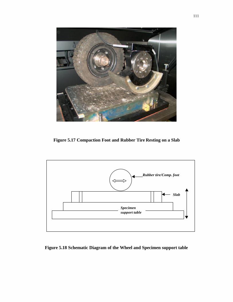
111
Figure 5.17 Compaction Foot and Rubber Tire Resting on a Slab
Figure 5.18 Schematic Diagram of the Wheel and Specimen support table
Rubber tire/Comp. foot
Slab
Specimensupport table
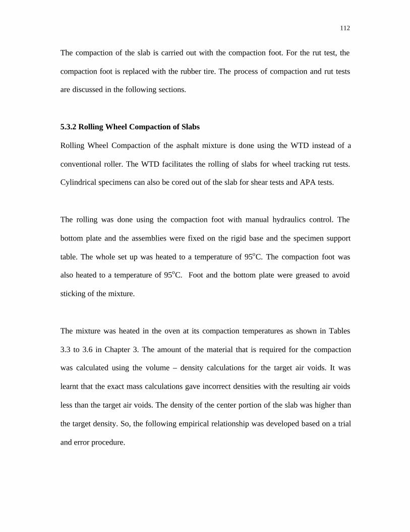
112
The compaction of the slab is carried out with the compaction foot. For the rut test, the
compaction foot is replaced with the rubber tire. The process of compaction and rut tests
are discussed in the following sections.
5.3.2 Rolling Wheel Compaction of Slabs
Rolling Wheel Compaction of the asphalt mixture is done using the WTD instead of a
conventional roller. The WTD facilitates the rolling of slabs for wheel tracking rut tests.
Cylindrical specimens can also be cored out of the slab for shear tests and APA tests.
The rolling was done using the compaction foot with manual hydraulics control. The
bottom plate and the assemblies were fixed on the rigid base and the specimen support
table. The whole set up was heated to a temperature of 95oC. The compaction foot was
also heated to a temperature of 95oC. Foot and the bottom plate were greased to avoid
sticking of the mixture.
The mixture was heated in the oven at its compaction temperatures as shown in Tables
3.3 to 3.6 in Chapter 3. The amount of the material that is required for the compaction
was calculated using the volume – density calculations for the target air voids. It was
learnt that the exact mass calculations gave incorrect densities with the resulting air voids
less than the target air voids. The density of the center portion of the slab was higher than
the target density. So, the following empirical relationship was developed based on a trial
and error procedure.

113
Mass (corrected) = Mass (exact)/ CSGC*1.01
where
Mass (corrected) = Required Mass of the mixture for compaction
Mass(exact) = Numerically calculated mass of the mixture for achieving target air voids
CSGC = Correction factor of the mixture when compacted using the SGC
The typical values of CSGC would range from 1.01 to 1.02. Mass calculated using this
relationship achieved the desired air void contents with a an acceptable range of ±.0.5%.
The mixture was compacted to a thickness of 75mm in three lifts. For the first lift, the
mixture was compacted to half the total thickness. For the subsequent lifts, the mixture
was compacted in two one-fourth of the remaining thickness. The slab was compacted in
more than two lifts to minimize gradient in the distribution of air voids. After each lift,
the surface of the compacted layer was scratched to prevent de-lamination of layers.
During the compaction process, the specimen support table was moved vertically with
slow and controlled movement to predetermined points. Predetermined heights (Z points)
are attributed to the thickness or top surface of the slab. The resistance offered by
compaction foot varies with the compactability of the mixture. The specimen support
table was moved in Y direction to compact the rear portion of the slab. To achieve a
uniform surface, the specimen support table was straddled across to prevent shoving of
the mixture on the other side of the slab. After compaction, the slab is allowed to cool
down. Nuclear gauge readings were then taken. For shear tests and APA tests, the
cylindrical specimens were cored out. Four specimens can be cored out from one slab.

114
The density of the specimens was measured using the water-displacement method for
verifying the target air voids.
5.3.3 Rutting Tests using the WTD
The rut tests were done on the RWC slabs and field slabs. RWC slabs were compacted
for all the mixtures whereas the field slabs were only available for the Charlotte and the
Kinston mixtures. The rut tests were performed at 60oC.
The top surface of the test slab was painted with water-soluble white traffic paint. The
surface was painted to prevent the effect of black surface that would cause interference
with laser measurement system at high temperatures. The compaction foot was replaced
with the rubber tire. The chamber was heated to a temperature of 60oC. Figure 5.19
shows a typical rut test being done on a test slab on a 75mm thick slab. The figure also
shows the rubber tire and the laser measurement system.
Figure 5.19 Typical Rut Test Using the NCSU WTD

115
The rut test was programmed to stop at a specific number of cycles or after the rut depth
reached its limit. The number of cycles selected for the test was 10,000 and the rut limit
was 1.5 inches. This rut limit includes the initial tire squeeze. Tire squeeze would
gradually decrease when the test proceeds. The profile of the slab was measured before
the commencement of the test and after every 1000 cycles. Laser measurement system
measures the depth at 180 points every time. Measurement was taken at 5 points
lengthwise and 36 points widthwise. Figure 5.20 shows the position of the measurement
points in both X and Y directions. A compressive load of 1000 lbs was applied against
the tire. The speed of the tire was selected as 30 passes/minute in one direction. The tire
movement was bi-directional and the effective tire speed was 60 passes/minute.
Figure 5.20 Laser Measurement Points on a Typical Slab
Measurement Points
-6
-4
-2
0
2
4
6
-6 -4 -2 0 2 4 6
X Direction
Y D
irect
ion

116
The rut tests were performed on RWC slabs for all the mixtures and field slabs for the
Charlotte and the Kinston mixtures. The rut depths measured at different points of the
slab were then analyzed. All the mixtures passed 10,000 cycles of loading without
reaching the rut limit of 1.5 inches. A few of the mixture specimens had rut depths above
0.5 inch as shown in Table 5.13. It would be interesting to know the number of cycles
that each mixture takes to reach 0.5 inch. So the number of cycles were interpolated from
the rut data as the measurements were taken only after every 1,000 cycles. Table 5.13
furnishes the final rut depth values at the end of 10,000 cycles. The rut depth values are
the average of profiles taken at 5 different sections of the slab in the X- direction. The
values in the parenthesis indicate the number of cycles required to reach a rut depth of 0.5
inch. Figure 5.21 compares the rut depth of different mixtures.
Table 5.13 Wheel Tracking Tests: Rut Depth
Mixture RWC Slabs, inch Field Slabs, inch
Auburn Coarse
Auburn Fine
Charlotte
Kinston
0.174
0.199
0.171
1.069 (2400)
N.A
N.A
0.607 (2300)
0.983 (700)
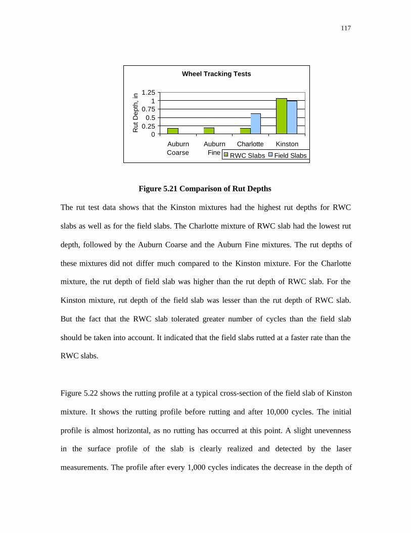
117
Figure 5.21 Comparison of Rut Depths
The rut test data shows that the Kinston mixtures had the highest rut depths for RWC
slabs as well as for the field slabs. The Charlotte mixture of RWC slab had the lowest rut
depth, followed by the Auburn Coarse and the Auburn Fine mixtures. The rut depths of
these mixtures did not differ much compared to the Kinston mixture. For the Charlotte
mixture, the rut depth of field slab was higher than the rut depth of RWC slab. For the
Kinston mixture, rut depth of the field slab was lesser than the rut depth of RWC slab.
But the fact that the RWC slab tolerated greater number of cycles than the field slab
should be taken into account. It indicated that the field slabs rutted at a faster rate than the
RWC slabs.
Figure 5.22 shows the rutting profile at a typical cross-section of the field slab of Kinston
mixture. It shows the rutting profile before rutting and after 10,000 cycles. The initial
profile is almost horizontal, as no rutting has occurred at this point. A slight unevenness
in the surface profile of the slab is clearly realized and detected by the laser
measurements. The profile after every 1,000 cycles indicates the decrease in the depth of
Wheel Tracking Tests
00.25
0.50.75
11.25
AuburnCoarse
AuburnFine
Charlotte KinstonR
ut D
epth
, in
RWC Slabs Field Slabs

118
the slab i.e., rutting has occurred. The heaps on right and left ends of the profile indicate
the lateral flow of the mixture when rutting has occurred.
Figure 5.22 A Typical Rutting Profile
In each of the 5 cross sections of the slab, points were selected at which maximum rutting
had occurred. The average of the change in rut depths after every 1,000 cycles at those
points was determined. Figures 5.23 to 5.28 show the rut depths of each mixture with
varying cycles of loading.
Figure 5.23: Rutting in Auburn Coarse Mixture (RWC slab)
Field Cores: Kinston
-1
-0.5
0
0.5
-6 -4 -2 0 2 4 6
Before Rutting After 10000 Cycles
RWC Slab: Auburn Coarse
-0.2-0.15
-0.1-0.05
00 2000 4000 6000 8000 10000
Cycles
Rut
Dep
th, i
n

119
Figure 5.24: Rutting in Auburn Fine Mixture (RWC slab)
Figure 5.25: Rutting in Charlotte Mixture (RWC slab)
Figure 5.26: Rutting in Kinston Mixture (RWC slab)
RWC Slab: Auburn Fine
-0.2-0.15-0.1
-0.050
0 2000 4000 6000 8000 10000Cycles
Rut
Dep
th, i
n
RWC Slab: Charlotte
-0.2
-0.15
-0.1
-0.05
00 2000 4000 6000 8000 10000
Cycles
Rut
Dep
th, i
n
RWC Slab: KINSTON
-2
-1.5
-1
-0.5
00 2000 4000 6000 8000 10000
Number of Cycles
Rut
Dep
th, i
n

120
Figure 5.27: Rutting in Charlotte Mixture (Field slab)
Figure 5.28 : Rutting in Kinston Mixture (Field slab)
The curves show that the rate of rutting was faster in the initial stages. For almost
all of mixtures, the rutting rate was faster in first 2,000 cycles, which gradually
decreased thereafter. The average rut depths at the end of 2,000 cycles are
summarized in Table 5.14. Figure 5.29 shows the comparison of rut depths at the
end of 2,000 cycles.
Field Slab: Charlotte
-2-1.5
-1-0.5
00 2000 4000 6000 8000 10000
Number of Cycles
Rut
Dep
th, i
n
Field Slab: Kinston
-2-1.5
-1-0.5
00 2000 4000 6000 8000 10000
Number of Cycles
Rut
Dep
th, i
n

121
Table 5.14 Rut Depths after 2000 Cycles
Mixture RWC Slabs, inch Field Slabs, inch
Auburn Coarse
Auburn Fine
Charlotte
Kinston
0.139
0.140
0.103
0.396
N.A
N.A
0.420
0.640
Figure 5.29: Rut Depths after 2000 Cycles
Rut Depths after 2000 Cycles
0
0.25
0.5
0.75
AuburnCoarse
AuburnFine
Charlotte Kinston
Rut
Dep
th, i
nch
RWC Slabs Field Slabs

122
At the end of 2000 cycles, the field slabs had higher rut depths than the RWC
slabs. It can be noticed that the field slabs reached almost 0.5-inch rut depth
around 2,000 cycles. The ratio of rut depth after 2,000 cycles and the rut depth
after 10,000 cycles of loading is calculated. The ratio is defined as the Initial Rut
Ratio, expressed in percentage. Table 5.15 shows the initial rut ratios for the
WTD rut tests.
Table 5.15 Initial Rut Ratio
Mixture RWC Slabs Field Slabs
Auburn Coarse
Auburn Fine
Charlotte
Kinston
79.9
70.4
60.2
37.0
N.A
N.A
80.1
77.3
Initial rut ratios show that almost 70 – 80% of the rutting occurred in the first
2,000 cycles for most of the mixtures. The Kinston mixture of RWC type, which
had the lowest percentage, reached 0.5 inch rut depth around 2,400 cycles. This
suggests that the terminal number of cycles for the WTD rut test can be decreased
from 10,000 cycles.
The rut depths show that the rolling wheel compaction provides mixtures with
superior performance as compared to the field slabs. The results of the wheel
tracking tests are compared with the APA tests and the repeated shear tests in
Chapter 6.
123
CHAPTER 6
MIXTURE PERFORMANCE ANALYSIS
Analysis of Service Life of Pavement
The resulting parameters of FSCH and RSCH tests are the material responses that can be
used to predict the pavement’s performance under service for distresses such as fatigue
cracking and rutting. Fatigue and Rutting analysis are performed using surrogate models
developed by SHRP 003-A project and distress models of Asphalt Institute. Fatigue
analysis of SHRP model considers material properties as well as pavement structural
layer thickness whereas rutting analysis considers only the material properties. In this,
chapter, the effects of the different compaction methods are studied in terms of its
performance to fatigue and rutting.
6. 1 SUPERPAVE Fatigue Model Analysis
The abridged fatigue analysis system from SHRP A-003A predicts the resistance of mix
to fatigue distress for a pavement structure under a given traffic load. The resistance of a
mix to fatigue cracking depends on the material properties such as initial flexural loss
stiffness and voids filled with asphalt (VFA) and the pavement structural property,
horizontal tensile strain at the bottom of the asphalt concrete layer. Shear stiffness of the
mixture is measured from the FSCH tests at 10 Hz at 20oC. The critical tensile strain is a
function of the pavement thickness.
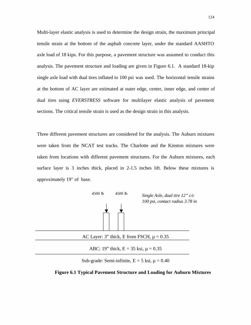
124
Multi-layer elastic analysis is used to determine the design strain, the maximum principal
tensile strain at the bottom of the asphalt concrete layer, under the standard AASHTO
axle load of 18 kips. For this purpose, a pavement structure was assumed to conduct this
analysis. The pavement structure and loading are given in Figure 6.1. A standard 18-kip
single axle load with dual tires inflated to 100 psi was used. The horizontal tensile strains
at the bottom of AC layer are estimated at outer edge, center, inner edge, and center of
dual tires using EVERSTRESS software for multilayer elastic analysis of pavement
sections. The critical tensile strain is used as the design strain in this analysis.
Three different pavement structures are considered for the analysis. The Auburn mixtures
were taken from the NCAT test tracks. The Charlotte and the Kinston mixtures were
taken from locations with different pavement structures. For the Auburn mixtures, each
surface layer is 3 inches thick, placed in 2-1.5 inches lift. Below these mixtures is
approximately 19" of base.
AC Layer: 3” thick, E from FSCH, µ = 0.35
ABC: 19” thick, E = 35 ksi, µ = 0.35
Sub-grade: Semi-infinite, E = 5 ksi, µ = 0.40
Figure 6.1 Typical Pavement Structure and Loading for Auburn Mixtures
4500 lb 4500 lb Single Axle, dual tire 12” c/c100 psi, contact radius 3.78 in

125
For the Charlotte mixtures, the surface layer is 2.4" thick (60mm) and below that is a
structural layer of 3.6" thick (90mm) with I19.0B. The ABC is 8" (200mm) thick.
AC Layer: 2.4” thick, E from FSCH, µ = 0.35
I19.0B 3.6” thick, E = 100 ksi, µ = 0.35
ABC: 8” thick, E = 35 ksi, µ = 0.35
Sub-grade: Semi-infinite, E = 5 ksi, µ = 0.40
Figure 6.2 Typical Pavement Structure and Loading for Charlotte Mixtures
AC Layer: 2.4” thick, E from FSCH, µ = 0.35
I19.0B: 3.2” thick, E = 100 ksi, µ = 0.35
ABC: 8” thick, E = 35 ksi, µ = 0.35
Sub-grade: Semi-infinite, E = 5 ksi, µ = 0.40
Figure 6.3 Typical Pavement Structure and Loading for Kinston Mixtures
4500 lb 4500 lb Single Axle, dual tire 12” c/c100 psi, contact radius 3.78 in
4500 lb4500 lb
Single Axle, dual tire 12” c/c100 psi, contact radius 3.78 in

126
For the Kinston mixtures, the pavement has 8" (200 mm) of ABC, 3.2" (80 mm) of
I19.0B, and 2.4" (60 mm) of surface mix.
The flexural properties of the mix are estimated using the following regression equations.
So = 8.56 * (Go)0.913 R2 = 0.712 (6-1)
So” = 81.125 * (Go”)0.725 R2 = 0.512 (6-2)
where
So = initial flexural stiffness at 50th loading cycle is psi
Go = shear stiffness at 10 Hz in psi
So” = initial flexural loss stiffness at 50th loading cycle is psi
Go” = shear loss stiffness at 10 Hz in psi
A summary of material properties are given in Table 6.1

127
Table 6.1 Summary of Estimated Material Properties for Various Mixes
Mixture Compaction |G*| psi Phase
Angle
Go' psi Go'' So' So''
Auburn
Coarse
Field Cores
RWC
SGC
2.30E+09
2.42E+09
2.39E+09
16.32
8.95
16.94
3.20E+05
3.47E+05
3.32E+05
9.37E+04
5.46E+04
1.01E+05
9.10E+05
9.78E+05
9.39E+05
3.26E+05
2.21E+05
3.45E+05
Auburn
Fine
Field Cores
RWC
SGC
1.96E+09
2.40E+09
2.98E+09
18.73
10.85
13.27
2.69E+05
3.42E+05
4.21E+05
9.13E+04
6.55E+04
9.92E+04
7.77E+05
9.66E+05
1.17E+06
3.20E+05
2.52E+05
3.40E+05
Charlotte Field Cores
RWC
SGC
9.45E+08
1.31E+09
1.44E+09
33.34
25.03
25.41
1.14E+05
1.72E+05
1.89E+05
7.53E+04
8.04E+04
8.96E+04
3.56E+05
5.16E+05
5.61E+05
2.79E+05
2.92E+05
3.16E+05
Kinston Field Cores
RWC
SGC
6.63E+08
1.21E+09
1.22E+09
37.51
24.76
23.07
7.63E+04
1.59E+05
1.63E+05
5.85E+04
7.35E+04
6.93E+04
2.46E+05
4.81E+05
4.91E+05
2.32E+05
2.74E+05
2.62E+05
The fatigue resistance of a mix is then estimated from the following strain-dependent
surrogate model.
Nsupply = 2.738E5* e 0.077VFB* ε0-3.624* S0” –2.72 (6-3)
where
Nsupply = estimated fatigue life of the given pavement section in ESALs
VFB = voids filled with asphalt
ε0 = critical tensile strain at the bottom of AC layer

128
The coefficient of determination for the surrogate model for fatigue analysis is 0.79 with
a coefficient of variation of 90 percent.
The results are summarized in Table 6.2 and compared in Figure 6.4.
Table 6.2 Summary of Fatigue Analysis Results (SHRP Surrogate Model)
Mixture Compaction So'' VFA Strain Nsupply Difference
Auburn Coarse Field Cores
RWC
SGC
3.26E+05
2.21E+05
3.45E+05
72.29 0.000154
0.000148
0.000151
4.75E+06
1.59E+07
4.36E+06
-
234 %
-8%
Auburn Fine Field Cores
RWC
SGC
3.20E+05
2.52E+05
3.40E+05
73.12 0.000167
0.000149
0.000134
3.93E+06
1.15E+07
7.43E+06
-
193 %
89%
Charlotte Field Cores
RWC
SGC
2.79E+05
2.92E+05
3.16E+05
77.48 0.000139
0.00014
0.00014
1.59E+07
1.34E+07
1.10E+07
-
-16%
-31%
Kinston Field Cores
RWC
SGC
2.32E+05
2.74E+05
2.62E+05
75.59 0.000132
0.000145
0.000145
2.69E+07
1.21E+07
1.36E+07
-
-55%
-49%

129
Figure 6.4 Comparison of Fatigue Life
For 12.5mm mixtures, RWC specimens had the longest fatigue life whereas for the
9.5mm mixtures, field cores had the longest fatigue life. Unlike the frequency sweep test
results, the results of fatigue analysis did not give a definite trend. The higher Nsupply
values of RWC specimens for the Auburn mixtures can be attributed to smaller phase
angles, which in turn decreased the flexural loss stiffness. The fatigue life of field cores
and SGC specimens of Auburn mixture were almost equal as were their corresponding
phase angles. For the 9.5mm mixtures, the fatigue life of field cores was longer than
those of laboratory compacted specimens. This behavior is attributed to the smaller
flexural loss stiffness values of field cores.
The shear stiffness values of the 12.5mm mixtures were almost double that of the 9.5mm
mixtures. Despite their higher stiffness values, the 12.5mm mixtures had shorter fatigue
life than the 9.5 mixtures due to their lower VFA values. Given the fact that each mixture
Fatigue Analysis
0.00E+00
1.00E+07
2.00E+07
3.00E+07
AC AF C KN
Sup
ply
FC RWC SGC

130
had different pavement structure, the ranking of mixtures in terms of their fatigue lives
would be inappropriate.
The number of cycles to failure under fatigue cracking is also estimated using Asphalt
Institute model. The allowable number of load repetitions is related to the tensile strain at
the bottom of the asphalt later, as indicated in the following equation.
Nf = 0.00796 * εt –3.291 * E1 –0.854 (6-4)
where,
Nf = allowable number of load repetitions to prevent fatigue cracking
(20% of area of crack)
εt = tensile strain at the bottom of asphalt later
E1 = elastic modulus of asphalt layer
The results are tabulated in Table 6.4

131
Table 6.4 Summary of Fatigue Analysis Results (AI Method)
Mixture Compaction Strain So' Nsupply
Auburn Coarse Field Cores
RWC
SGC
1.54E-04
1.48E-04
1.51E-04
9.10E+05
9.78E+05
9.39E+05
2.30E+05
2.46E+05
2.36E+05
Auburn Fine Field Cores
RWC
SGC
1.67E-04
1.49E-04
1.34E-04
7.77E+05
9.66E+05
1.17E+06
2.00E+05
2.43E+05
2.91E+05
Charlotte Field Cores
RWC
SGC
1.39E-04
1.40E-04
1.40E-04
3.56E+05
5.16E+05
5.61E+05
7.22E+05
5.04E+05
4.77E+05
Kinston Field Cores
RWC
SGC
1.32E-04
1.45E-04
1.45E-04
2.46E+05
4.81E+05
4.91E+05
1.16E+06
4.75E+05
4.68E+05
The AI method of fatigue analysis indicated that field cores of the Charlotte and the
Kinston mixtures had longer fatigue life than the laboratory compacted specimens. For
12.5 mixtures, there was no significant difference among the three methods of
compaction. SHRP fatigue model considers tensile strain, loss flexural modulus and
voids filled with asphalt whereas the AI model considers only the tensile strain and the
modulus of elasticity. So SHRP fatigue model provides more dependable results than the
AI model.
132
6.2 SUPERPAVE Rutting Model Analysis
The permanent deformation system of SHRP A-003A estimates rut depth from the
maximum permanent shear strain obtained from RSCH test using the following relation.
Rut depth (in.) = 11 * Maximum permanent shear strain (6-5)
If rutting in millimeters is desired, the coefficient of the above equation is about 275. The
above relationship is obtained for a tire pressure of 100psi and asphalt layer thickness of
15inch. Studies (3) performed for the similar pavement structure at 200psi and 500psi
suggest that this relationship is independent of the tire pressure. But the same is not true
in the case of pavement thickness. The coefficient is expected to decrease with a decrease
in asphalt layer thickness.
The conversion of the number of RSCH test cycles to ESALs is determined by the
following equation:
log (cycles) = -4.36 + 1.24 log (ESALs) (6-6)
where,
cycles = number of cycles obtained from the RSCH test
ESALs = equivalent 18-kip single axle load
According to the above relationship, 5000 cycles of the RSCH test correspond to 3.156
million ESALs. The summary of the results are given in Table 6.5 and compared in
Figure 6.5

133
Table 6.5 Summary of Rutting Analysis Results (SHRP Surrogate Model)
Mixture Compaction Shear Strain Rut Depth Cycles NSupply
Auburn Coarse Field Cores
RWC
SGC
0.0270
0.0163
0.0132
0.30
0.18
0.15
5000
5000
5000
> 3156232
> 3156232
> 3156232
Auburn Fine Field Cores
RWC
SGC
0.0245
0.0180
0.0150
0.27
0.20
0.17
5000
5000
5000
> 3156232
> 3156232
> 3156232
Charlotte Field Cores
RWC
SGC
0.0455
0.0210
0.0129
0.50
0.23
0.14
802
5000
5000
721440
> 3156232
> 3156232
Kinston Field Cores
RWC
SGC
0.0455
0.0455
0.0283
0.50
0.50
0.31
677
3300
5000
629306
2257563
> 3156232
Figure 6.5 Comparison of Rut Depths
The results of rutting analysis clearly showed that the rut susceptibility of field cores was
generally higher than RWC specimens and SGC specimens. The rut depths of RWC
Rutting Analysis
0.000.20
0.40
0.60
AC AF C K
Rut
dep
th, i
n
FC RWC SGC

134
specimens were higher than the rut depths of SGC specimens. This trend is noticed in all
mixtures, irrespective of the nominal maximum size of aggregate or gradation. In other
words, it is evident that SGC specimens provided lower rut depths as compared to field
cores. It should be borne in mind that there is no difference in air voids among the
different methods of compaction as the laboratory specimens were compacted at the
corresponding average densities of field cores for different mixtures. The rolling wheel
compacted specimens seemed to better simulate the field conditions than the Superpave
Gyratory Compactor.
In addition, the rutting model of Asphalt Institute was utilized for investigating the rutting
resistance of the mixtures since the rutting distress model developed by the SHRP
program depends only on the mixture properties. In the AI distress model, the allowable
number of load repetitions (Nd) to limit rutting (0.5 inch) is related to the vertical
compressive strain at the top of subgrade (εc) by the following relationship:
Nd = 1.365 x 10-09 * εc-4.477 (6-7)
The vertical compressive strain at the top of subgrade was estimated using
EVERSTRESS pavement analysis software. The estimated number of cycles to failure
under rutting for all mixtures are given in Table 6.6

135
Table 6.6 Summary of Rutting Analysis Results (AI Method)
Mixture Compaction Shear Strain Nd
Auburn Coarse Field Cores
RWC
SGC
4.70E-04
4.66E-04
4.68E-04
1079545
1123575
1098346
Auburn Fine Field Cores
RWC
SGC
4.79E-04
4.67E-04
4.55E-04
992807
1115408
1247194
Charlotte Field Cores
RWC
SGC
8.90E-04
8.50E-04
8.42E-04
62180
76270
79569
Kinston Field Cores
RWC
SGC
9.75E-04
9.02E-04
9.00E-04
41244
58435
59019
The analysis show that the SGC specimens tolerated higher number of load repetitions
than the field cores. There seemed to be no significant difference between the results of
SGC and RWC specimens. The AI method of rutting analysis utilizes only the flexural
modulus of mixtures. The analysis using the AI model is based on the elastic analysis of
the pavement structure and the rutting is governed by the compressive strain at the top of
the subgrade. In other words, the AI model is predicated on the assumption that rutting is
controlled by the deformation of the subgrade. On the other hand, the SHRP model
assumes that rutting is more pronounced in the surface layers and, therefore, the mixture

136
properties of the surface layer primarily dictate the rutting behavior of a given pavement.
As this study involved the evaluation of the mixtures with respect to their rutting
potential, the SHRP rutting model was employed for this purpose
6.3 Correlation of APA Test Results
Permanent deformation or rutting in asphalt concrete pavements can be measured using
different performance evaluation procedures. The commonly used procedures, as
indicated by the literature (20) are as follows:
§ Diametral tests
§ Uniaxial tests
§ Triaxial tests
§ Shear tests
§ Empirical tests (Marshall test, Hveem test etc)
§ Simulative tests (APA, PurWheel, HWTD, MMLS etc)
Among these, shear tests, empirical tests and simulative tests are more common. Shear
tests, though fundamental, are very expensive, complicated and unreasonable for QC
testing. Empirical tests such as Marshall test, Hveem test etc have been used for years
with limited success. Simulative tests such as APA are simple, easy to perform. Literature
shows reasonable correlation between the test results and field performance.
One of the objectives of this study was to investigate how the mixture performance as
measured by the APA correlates with that of the other performance evaluation procedures

137
and devices. The tests results as measured by the APA were compared with the RSCH
test results and NCSU WTD test results. The NCSU WTD rut test is an accelerated wheel
tracking tests that falls in the category of simulative tests. The WTD device has certain
advantages over other simulative tests. The device uses rolling wheel compacted slabs
and field slabs. The load is applied to through a rubber tire similar to a pneumatic tire
used in vehicles.
Table 6.7 summarizes the test data as measured by the APA, RCSH and WTD rut tests.
The data are converted into same scale (inches), as these test systems measure in different
units such as mm and inch. Rut depths of APA measured in mm are converted to inches.
Table 6.7 Rut Depths (inches)
Field Compaction RWC SGCMixture
Shear APA WTD Shear APA WTD Shear APA
Auburn Coarse
Auburn Fine
Charlotte
Kinston
0.30
0.27
0.50*
0.50*
0.195
0.429
0.755
0.627
N.A
N.A
0.607
0.983
0.18
0.20
0.23
0.50*
0.197
0.332
0.262
0.479
0.174
0.199
0.171
1.069
0.15
0.17
0.14
0.31
0.101
0.220
0.168
0.477
(*) Mixture reaches the limit and further test is stopped
The mixtures that reached the limit in shear tests were the Charlotte (FC), the Kinston
(FC) and the Kinston (RWC). These mixtures had experienced the maximum allowable
rut depth of 0.5 inch. The mixtures failed at different number of cycles (below 5000)
which triggered the termination of the test. The corresponding rut depths of failed

138
mixtures, measured using the APA or WTD, had either crossed 0.5 inch or almost
reached 0.5 inch of rutting. None of the mixtures that passed the repeated shear tests had
reached 0.5 inch of rutting. This fact explains the good correlation among the different
test systems. Therefore, it seems that like the shear tests, the simulative tests such as the
NCSU WTD or the APA can also effectively detect poorly performing mixtures.
Different parameters established using the test systems in this study were correlated with
each other. The strength of the correlation is measured using the coefficient of multiple
determination (R2). The corresponding data of two parameters were plotted on a scatter
plot and the regression equation of the relationship was also determined.
The rut depths measured using the APA tests are related with the rut depths estimated
using the shear test data. The rut depth calculated using the SHRP Surrogate models is a
simple multiplication of the corresponding shear strain by 11. Figure 6.6 shows the
scatter plot between the rut depths as measured using the APA and shear tester.
Figure 6.6 Correlation of RSCH Rut Depth and APA Final Rut Depth
RSCH (Rut Depth) vs APA (Rut Depth)
y = 1.268x - 0.0097R2 = 0.7755
00.10.20.30.40.50.60.70.8
0 0.1 0.2 0.3 0.4 0.5 0.6RSCH Rut Depth, inch
AP
A R
ut D
epth
, inc
h

139
It should be borne in mind that the RSCH rut depths of failed mixtures remain at 0.5 inch,
though the mixtures failed at different number of cycles. In spite of the above fact, the R2
value of 0.78 indicates a reasonably strong correlation between APA tests and shear tests.
It was observed from the APA tests that the initial rate of deformation was higher than
the final rate of deformation. The rut depth after 1000 cycles was taken into account
along with the final rut depth after 8000 cycles. The rut depth after 1000 cycles as
measured by the APA were correlated with the rut depths estimated by the shear tests.
Figure 6.7 shows the scatter plot between the rut depths after 1000 cycles with rut depths
of shear test data.
The correlation between the APA rut depths after 1000 cycles and rut depths of shear
tests are strong. The R2 value of this relationship is about 0.78, almost equal to that of the
final rut depth after 8000 cycles.
Figure 6.7 Correlation of RSCH Rut Depth and APA Initial Rut Depth
RSCH(Rut depth) vs APA (Rut Depth)
y = 1.2099x - 0.1466
R2 = 0.7825
0
0.1
0.2
0.3
0.4
0.5
0.6
0.7
0 0.2 0.4 0.6
RSCH Rut Depth, inch
AP
A R
ut D
epth
(10
00),
in
ch

140
The mixtures of RWC type were tested using the APA and the NCSU Wheel Tracking
Device. Though the limited number of data points, the rut depths of APA and WTD were
correlated. Figure 6.8 shows this correlation in terms of the scatter plot between the APA
final rut depth and WTD final rut depth. The R2 value of the relationship was 0.81. This
indicates a reasonale correlation between the predictability of the APA and the NCSU
WTD.
Figure 6.8 Correlation of WTD and APA Final Rut Depth of RWC
It was observed from the NCSU WTD test data that about 80% of the total rutting occurs
in the first 2000 cycles. The rut depths after 2000 cycles were measured by the NCSU
WTD were correlated with the APA rut depths after 1000 cycles. Figure 6.9 shows the
scatter plot between the initial rut depths of APA and NCSU WTD. The R2 value of 0.79
indicates a strong correlation between the initial rut depths of the APA and the NCSU
WTD.
APA (RWC) vs WTD (RWC)
y = 3.3099x - 0.6478R2 = 0.8121
00.20.40.60.8
11.2
0 0.1 0.2 0.3 0.4 0.5 0.6
APA Rut Depth, inch
WT
D R
ut D
epth
, inc
h

141
Figure 6.9 Correlation of Initial Rut Depths of APA and WTD
The WTD rut depths for the field slabs as well as the RWC slabs were correlated with the
rut depths estimated using the shear test data. Figure 6.10 shows the scatter plot between
the rut depths of WTD and Shear tester. The R2 value of the above correlation is 0.85,
which also indicates the existence of a reasonable correlation between the two test
systems.
Figure 6.10 Correlation of RSCH Rut Depth and WTD Final Rut Depth
Rut Depth: RSCH vs WTD
y = 2.3461x - 0.2905R2 = 0.8502
00.20.40.60.8
11.2
0 0.1 0.2 0.3 0.4 0.5 0.6
RSCH Rut Depth, inch
WT
D R
ut D
epth
, inc
h
Initial Rut Depth: APA vs WTD
y = 0.9917x - 0.1205R2 = 0.786
0
0.1
0.2
0.3
0.4
0.5
0 0.1 0.2 0.3 0.4 0.5 0.6
APA Rut Depth (1000), inch
WTD
Rut
Dep
th (
2000
), in
ch

142
The R2 values of all the relationships are above 0.75. This indicates that a strong
correlation exists among the test results as measured by the Shear tester, the APA and the
NCSU WTD. This supports the fact that simulative tests such as APA and the NCSU
WTD can be used to detect poorly performing mixtures as effectively as the shear tests.

143
CHAPTER 7
SUMMARY OF RESULTS AND CONCLUSIONS
A laboratory mix design system aids in predicting the in-service performance of the
asphalt mixtures through various performance evaluation tests. The compaction methods
adopted in the laboratory for specimen fabrication are expected to simulate the properties
of the pavement in the field. The physical properties of the specimens depend on the
method of compaction used for fabrication. It is desirable that the laboratory compaction
of specimens should be a true indicator of field performance. The effects of different
compaction methods on the performance of mixtures have been investigated in this study.
The central objective of this study was to evaluate as to how the different compaction
methods affect the performance of the mixtures. Laboratory compaction methods such as
Superpave Gyratory Compaction (SGC) and Rolling Wheel Compaction (RWC) were
compared with the field compaction. Four field mixtures had been selected for this
purpose. Loose mixtures from the test sites were utilized for laboratory compaction of
mixtures. The mixtures were identified as Auburn Coarse, Auburn Fine, Charlotte and
Kinston. The Auburn mixtures were 12.5mm mixtures whereas the Charlotte and the
Kinston mixtures were 9.5mm mixtures.
The performance parameters of the mixtures include fatigue and rutting distresses.
Permanent deformation or rutting in hot mix asphalt pavements is caused by the
consolidation or lateral movement, or both, of the HMA under traffic. The rutting

144
susceptibility of the mixtures was investigated using fundamental test method such as
Shear test and simulative tests using the APA and the NCSU WTD. The results of these
test systems were compared and correlated.
Compaction characteristics of the individual mixtures were studied using the Superpave
Gyratory Compactor and the Gyratory Load-Cell Plate Assembly (GLPA). Densification
of mixtures obtained from the SGC revealed that no mixture had four percent air voids at
design number of gyrations. Percent Air at Ndes was around 3% for the Auburn mixtures,
whereas the percent air values were 6.3% and 4.9% for the Charlotte and the Kinston
mixtures, respectively. The Charlotte mixture did not reach four- percent voids even at its
maximum number of gyrations. The slopes of the compaction curves of the mixtures
were computed. The compaction slope is an indication of an aggregate structure’s
resistance to compaction. Since the SGC operates as a gyratory shear compactor, the
slope of the compaction curve might be considered related to the shear resistance of the
aggregate structure. In this regard, the Auburn Coarse mixture had the highest
compaction slope whereas the Kinston mixture had the lowest compaction slope. The
slopes of the Auburn Fine mixture and the Charlotte mixture were similar to each other.
The compaction slopes seemed to suggest that the Auburn Coarse mixture had the highest
shear resistance and the Kinston mixture had the lowest shear resistance among all the
mixtures.
The mixtures were compacted using the SGC and the GLPA for the computation of
energy indices. The volumetric properties estimated using the Pine SGC agreed with

145
those properties estimated using the Troxler SGC. The Auburn mixtures were gyrated to
160 gyrations while the Charlotte and the Kinston mixtures were gyrated to 600
gyrations. The Charlotte mixture did not reach 98 percent of its maximum theoretical
density even after 600 gyrations.
The energy indices, Construction indices and Traffic indices, are the measures of
densification and distortion under construction and under traffic. As per the definition,
the construction indices are the integration of the area under the densification curve
between the first gyration and the 92% Gmm. On the other hand, the traffic indices are the
integration of the area under the densification and resistive work curves between
92%Gmm and 98% Gmm.
The Compaction Densification Index (CDI) and Compaction Force Index (CFI) are used
to evaluate the performance of mixtures during construction. This effort is the work
applied by the pavers/rollers to compact the mix to the required density during
construction. Mixes that require lower compaction energy are desirable. The compaction
indices indicate that the Charlotte mixture is the harshest mixture to compact. The
Kinston mixture follows next. The Auburn mixtures have lower indices than other
mixtures. The Auburn Fine is the most desirable mixture for compaction followed by the
Auburn Coarse.
The Traffic Densification Index (TDI) and Traffic Force Index (TFI) are used to evaluate
the performance of mixtures during traffic. Higher traffic indices indicate that the mixture

146
would require more traffic to reach their terminal density and, in other terms, longer rut
life. The traffic indices show very high values for the Charlotte and the Kinston mixtures
and very low values for the Auburn mixtures. A possible explanation could be that the
Charlotte and the Kinston mixtures being harsh took more number of gyrations to reach
98 percent of their maximum theoretical density. Obviously, the Auburn mixtures were
easier to compact given that the mixtures reached their 98 percent Gmm in fewer
gyrations. The compactability of the mixtures severely influenced the values of traffic
indices. However, the traffic indices (TDI and TFI) do not adequately explain the rutting
potential of the mixtures with different sources of aggregates. Therefore, the reverse trend
between the construction indices and traffic indices was not observed, as the aggregate
sources of these mixtures remained different. The interpretation of rutting characteristics
of mixtures from their traffic indices was not attempted due to these discrepancies.
In order to evaluate the effect of different compaction methods, various performance
evaluation tests were conducted on the field cores and specimens fabricated using the
SGC and RWC. Performance evaluation was done using test systems such as Shear
tester, APA and NCSU WTD. The results of FSCH and RSCH tests were then analyzed
using the SHRP A 003-A surrogate models and the Asphalt Institute (AI) method. The AI
method considers only the mixture stiffness; on the other hand, surrogate models use
various mixture properties such as shear strain, flexural stiffness and voids filled with
asphalt. Therefore, the results of SHRP surrogate models are considered more dependable
and are given more credence for the purpose of this discussion.

147
The FSCH test measured dynamic modulus and phase angles at 20oC and at various
frequencies. The values of dynamic modulus (G*) at 10Hz showed that the 12.5mm
mixtures were stiffer than the 9.5mm mixtures. The same behavior was noticed for all the
three methods of compaction. The gyratory compacted mixtures had the highest stiffness
followed by the rolling wheel compacted mixtures. The field cores had lowest stiffness
values for all four mixtures. The estimates of fatigue life do not agree with the trend
shown by the dynamic modulus. The RWC mixtures had the longest fatigue life for the
Auburn mixtures and on the other hand, the field cores had the longest fatigue life for the
Charlotte and the Kinston mixtures. For the Auburn mixtures, the fatigue lives of field
cores and SGC mixtures were almost equal. For the Charlotte and the Kinston mixtures,
the fatigue lives of RWC and SGC mixtures were almost equal. The reason for the above
mixed trend can be attributed to the trend of phase angles. For the Auburn mixtures, the
phase angles of RWC were the lowest. For the Charlotte and the Kinston mixtures, the
phase angles of RWC and SGC were almost the same, whereas the phase angles of the
field cores were the highest. Higher phase angles increase the loss flexural modulus of
the mixtures and the critical tensile strain at the bottom of the AC layer. This, in turn,
decreases the fatigue life of the mixtures. Thus the phase angles attributed to the mixed
trend of fatigue life of the mixtures.
The shear strains were measured using the RSCH test. The rut depths were estimated
using the SHRP Rutting model. The Auburn mixture specimens prepared with all of the
compaction types passed the 5000-cycle criteria. The field cores and RWC specimens of
the Kinston mixtures failed at 677 and 3300 cycles of loading, respectively. For the

148
Charlotte mixtures, the field cores failed early at 802 cycles of loading while the
laboratory compacted specimens passed the shear tests and their shear strains were very
low. The shear strain of the SGC specimens was the lowest among the three-compaction
methods for all the mixtures. The shear strains of RWC specimens are higher than those
of SGC specimens. The field cores had the highest shear strain of all the mixtures. The
results of the RSCH test show that specimens fabricated using the SGC tend to provide
superior performance. The rolling wheel compaction, whose results are in between the
SGC and field cores, seems to simulate field conditions better than the SGC.
Rutting characteristics of the mixtures were also measured using the Asphalt Pavement
Analyzer (APA). The rut depths were measured at the end of 8000 cycles. The results of
the APA tests showed that the SGC specimens had the lowest rut depths. The rut depths
of the field cores were higher than the rut depths of the RWC specimens. The field cores
of the Charlotte mixture rutted more severely than the RWC and SGC specimens. These
results seemed to be in agreement with the RSCH test results.
As the initial rate of deformation was higher than the final rate of deformation in the APA
tests, the rut depths at the end of 1000 cycles were determined which demonstrated the
initial rutting behavior of the mixtures. The results show that the rut depths of SGC
specimens had the lowest rut depths, followed by the RWC specimens. Field cores
exhibited very high rut depths at the end of 1000 cycles. The Initial Rut Ratio, the ratio of
the rut depth after 1000 cycles to the rut depth after 8000 cycles, was calculated for all
the mixtures. The initial rut ratio seems to be influenced by the maximum size of the

149
aggregate and the type of compaction method. In general, the 12.5mm mixtures have
lower initial rut ratios than the 9.5mm mixtures. Field cores have the highest initial rut
ratios whereas the SGC samples have the lowest initial rut ratios. For RWC samples, the
initial rut ratios are found in between the initial rut ratios of field cores and SGC samples.
This ratio could be a measure of the initial rutting resistance offered primarily by the
aggregate skeleton of a mixture.
The results of the APA tests were used to estimate the viscoelastic parameters such as E
and viscosity (η) using the Kelvin model. The estimated E value is not the real modulus
of elasticity but could be considered as a “pseudo” modulus. The retardation time, tc, at
which 63 % of the total strain occurs, was also calculated. The retardation times of the
SGC mixtures were greater than the retardation times of RWC specimens and field cores.
The results of the APA tests showed that the field cores had the higher rutting potential
than the RWC specimens and the SGC specimens for all mixtures. The same trend was
seen in the results and the estimates of the APA tests and the RSCH tests. The gyratory
compaction provides specimens that tend to overestimate the field performance. The
rolling wheel compaction of specimens seems to simulate field conditions better than the
SGC.
The NCSU WTD rut tests were performed on RWC slabs of all mixtures and field slabs
of the Charlotte and the Kinston mixtures. Field slabs of these mixtures produced deeper
ruts than the RWC slabs at the end of 10000 cycles. Initial rut depths at the end of 2000

150
cycles produced a similar trend. Initial rut ratios showed that field slabs rutted faster than
roller compacted slabs.
In general, the results of the rutting tests evaluated using the RSCH, APA and NCSU
WTD indicated the same trend. The specimens fabricated using the SGC had lowest rut
depths, followed by the RWC. The field specimens not only had highest rut depths but
also rutted faster than the laboratory fabricated specimens. The Superpave Gyratory
Compaction (SGC) tends to provide better performance and under predicts the field
rutting potential. The Rolling Wheel Compaction (RWC) seems to simulate more realistic
field compaction and produce field conditions better than the SGC. It is evident that the
method of compaction has a profound influence on the performance of the mixtures. This
fact could be possibly due to the difference in the internal structure of the compacted
mixes, as explained in the literature. The differences in the distribution of air voids and
aggregates orientation inside the mixture are referred to as the internal structure. Rolling
wheel compacted specimens would be expected to have increasing air void contents from
top to bottom of the lift, as do field specimens (8). Air void contents are expected to be
fairly homogeneous in the horizontal plane of the rolling wheel. However for the SGC,
the middle of the SGC specimen is compacted more than the top and the bottom, and the
interior of the specimen is expected to become better compacted than the exterior (9).
The accelerated performance tests are simple, inexpensive and require less expertise than
the fundamental tests such as the Shear tests. One objective of this study was to find
whether performance evaluation devices such as APA could clearly detect poorly

151
performing mixtures. The results of the APA tests were correlated with the results of the
RSCH test and the NCSU WTD. When the results of all the test systems were converted
to a same scale of inches and summarized, the comparison reveals that the mixtures that
had failed in the RSCH test had rut depths greater than 0.5 inch in APA and NCSU
WTD. Interestingly, none of the mixtures that passed the RSCH test had rut depths
greater than 0.5 inch in other test systems either. These observations strongly suggest that
the rut depth of 0.5 inch could be opted as “pass/fail” or “go-no go” criteria for APA
tests.
The results of the APA and RSCH tests were correlated. The R2 value of 0.78 indicates a
reasonably strong correlation between the two tests despite the fact that the RSCH test
uses 0.5 inch as rut depth for all failed mixtures. During the RSCH test, a mixture fails
when it reaches the maximum shear strain. The failure occurs at different number of
cycles for different mixtures. However, the SHRP rutting model estimates a rut depth of
0.5 for all failed mixtures even though the mixtures had failed at different cycles of
loading. If the failed mixtures are allowed to 5000 cycles of loading, the shear strains as
well as the rut depths would be much higher and a better correlation can be expected.
The results of APA and NCSU WTD tests on RWC specimens were also correlated. The
R2 value of the relationship was 0.81. This again, indicates a strong correlation between
the predictability of the APA and the NCSU WTD. This correlation was done with
limited availability of test data. The correlations among the different test parameters of
RSCH, NCSU WTD and APA strongly support the premise that the predictability of the

152
accelerated tests is as appealing as the fundamental tests like Shear tests. The APA can
also detect poorly performing mixtures as one of the performance evaluation devices.
The performance evaluation tests were conducted at the densities of the field cores. The
laboratory-fabricated specimens were compacted to the average density of the field cores.
The air voids of the individual mixtures were different. One of the objectives of this
study was to evaluate how changes in aggregate and asphalt source would affect the
performance of the mixtures. For this purpose the mixtures were compacted to 4 percent
air voids using the SGC, so that a meaningful comparison could be done. The Auburn
Coarse mixture has the highest G* among all the mixtures followed by the Auburn Fine,
the Charlotte and the Kinston mixtures. The RSCH test results show that the Kinston
mixture had the highest shear strain among all the mixtures. The shear strains of the
Auburn mixtures and the Charlotte did not differ significantly at four percent air voids.
Conclusions
In summary, the following principal conclusions can be drawn.
1. The laboratory compacted mixtures tend to be superior in their performance than the
field cores. In other words, the laboratory compaction by SGC results in under
prediction of the field rutting potential of the mixtures. The mixtures compacted using
the SGC and the RWC have higher stiffness values and lower shear strain values than
the field cores. The Rolling Wheel Compaction (RWC) seems to simulate field
compaction better than the SGC.

153
2. There exists a good correlation among the results of the RSCH tests, the APA tests
and the NCSU WTD rut tests. The mixtures, which failed to satisfy the RSCH test
criteria, had rut depths greater than 0.5 inch, as measured by the APA and NCSU
WTD. The mixtures that passed the RSCH tests had rut depths less than 0.5 inch.
3. The APA test can detect poorly performing mixtures as well as some of the other
performance evaluation devices. It is suggested that a rut depth of 0.5 inch could be
prescribed in the APA test as “pass/fail” or “go-no go” criteria. This suggested value
of 0.5 inch is based on the test data of the four mixtures included in this study.
However, more mixtures should be involved for this evaluation to get a better
estimate of limiting value of rutting.
4. The NCSU WTD test can also be used as a simulator to examine the rutting
susceptibility of a mixture. It seems that the same criterion of 0.5-inch rut depth is
suitable for the NCSU WTD also.
5. When the mixtures were examined at four percent air voids, the test results indicated
that the Auburn mixtures (12.5-ARZ and 12.5-BRZ) had higher G* values at 10 Hz
than the Charlotte (9.5-BRZ) and the Kinston mixtures (9.5-ARZ). The RSCH test
results indicated that the Kinston mixture had the highest rutting potential among all
the mixtures. The rutting characteristics of other mixtures were almost similar.
6. Construction indices, as measured by the SGC and the GLPA, showed that the
Auburn mixtures were more desirable from construction standpoint as these mixtures
appeared to be easy to compact. The Charlotte mixture was the most difficult mixture
to compact followed by the Kinston mixtures. The performance evaluation of the
mixtures using the traffic indices was not attempted in this study.
154
REFERENCES
1. Philip B. Blankenship et al, “Rational Method for Laboratory Compaction of Hot-
Mix Asphalt”, Transportation Research Record 1454, pp 144-153.
2. M.N Partl and L.Francken, “Basic Elements of a Testing Methodology for
Bituminous Materials and significant features for testing”, Bitumious Binders and
Mixes, Report of RILEM Techinical Committee 152 PBM, pp 1-10.
3. Carl. M. Monismith, “Asphalt Concrete: An Extraordinary Material for Engineering
Applications”, Thirtieth Henry M. Shaw Lecture, North Carolina State University.
4. Gerald A. Huber, “Development of the Superpave Gyratory Compactor”,
http://www.utexas.edu/research/superpave/articles/gyr_hist.html
5. B.A. Vallerga, “Recent Laboratory Compaction Studies of Bituminous Paving
Mixtures”, Proc. Association of Asphalt Paving Technologists, Vol 21, 1951, pp.117-
153
6. Von Quintus et al, “Comparative Evaluation of Laboratory Compaction Devices
Based on Their Ability to Produce Mixtures with Engineering Properties similar to
those produced in the Field,” Transportation Research Record 1228, pp 80-87.
7. Joe W. Button et al, “Correlation of Selected Laboratory Compaction Methods with
Field Compaction”, Transportation Research Record 1454, pp 193-201
8. John Harvey et al, “Effects of Laboratory Specimen Preparation on Aggregate-
Asphalt Structure, Air-Void Content Measurement, and Repetitive Simple Shear Test
Results,” Transportation Research Record 1454, pp 113-122.
9. Eyad Masad, “Quantifying Laboratory Compaction Effects on the Internal Structure
of Asphalt Concrete”, Transportation Research Record 1681, pp 179-185.
155
10. Brian J Coree and Kera VanDerHorst, “Superpave Compaction”, Crossroads 2000,
Tranportation Conference Proceedings, pp 264-267
http://www.ctre.iastate.edu/pubs/crossroads/264superpave.pdf
11. Bahia, H., Friemel, Timothy, Peterson, Pehr and Russell, Jeffrey. Optimization of
Constructability and Resistance to Traffic: A New Design Approach for HMA Using
the Superpave Compactor. Proc., Association of Asphalt Paving Technologists, Vol
67, 1998, p 189
12. L.A. Cooley Jr., P.S. Kandhal, M.S. Buchanan, F. Fee, & A. Epps, “Loaded Wheel
Testers In the United States: State of the Practice”, NCAT Report No 2001-04,
Transportation Research E-Circular E-C016, July, 2000.
http://www.nas.edu/trb/publications/circulars/ec016.pdf.
13. Lai, J. S. “Evaluation of Rutting Characteristics of Asphalt Mixes Using Loaded
Wheel Tester”. Project No. 8609, Georgia Department of Transportation, Dec. 1986.
14. Collins, R., H. Shami, and J. S. Lai. “Use of Georgia Loaded Wheel Tester To
Evaluate Rutting of Asphalt Samples Prepared by Superpave Gyratory Compactor”,
Transportation Research Record 1545, TRB, National Research Council, Washington,
D.C., Nov. 1996, pp. 161-168.
15. Kandhal, P. S., and R. B. Mallick. “Evaluation of Asphalt Pavement Analyzer for
HMA Mix Design.” NCAT Report No. 99-4, National Center for Asphalt
Technology, June1999.
16. Aschenbrener, T. “Evaluation of Hamburg Wheel-Tracking Device to Predict
Moisture Damage in Hot Mix Asphalt”, Transportation Research Record 1492,TRB,
National Research Council, Washington, D.C., July 1995, pp. 193-201.

156
17. Hall, K. D. and S. G. Williams, "Effects of Specimen Configuration andCompaction
Method on Performance in Asphalt Concrete Wheel-Tracking Tests", Presented to the
Canadian Technical Asphalt Association, June 1, 1999.
18. Bonnot, J. “Asphalt Aggregate Mixtures”, Transportation Research Record 1096,
TRB, National Research Council, Washington, D.C., 1986, pp. 42-51.
19. Epps, A., T. Ahmed, M. Mikhail, and F. Hugo, “Performance Prediction with the
MMLS3 WesTrack” Paper to be submitted for publication in the Journal of the
Association of Asphalt Paving Technologists, March 19-21, 2001.
20. Brown, E.R., Kandhal, P.S., Jingna Zhang, “Performance Testing for Hot Mix
Asphalt (Executive Summary), NCAT Report No 2001-05 A, Nov 2001
http://www.eng.auburn.edu/center/ncat/reports/rep01-05A.pdf
21. Superpave Level 1 Mix Design, Superpave Series No.2 (SP-2), Asphalt Institute,
Lexington.
22. R. Michael Anderson and Hussian U. Bahia, “Evaluation of Aggregate Gradation for
Asphalt Mixtures,” Transportation Research Record 1583,TRB, National Research
Council, Washington, D.C., 1997, pp. 91-97
23. Rajib B.Mallick, “Use of Superpave Gyratory Compactor to Characterize HMA”,
Transportation Research Record 1681,TRB, National Research Council, Washington,
D.C., 1999, pp. 86-96
24. Guler, M, Bahia, HU, Bosscher, PJ., and Plesha, ME., “Device for Measuring Shear
Resistance of Hot-Mix Asphalt in Gyratory Compactor”, Transportation Research
Record 1723, 2000, pp 116-124.

157
25. Stakson A.D., Bushek, J.J. and Hussian U. Bahia, “Effect of Fine Aggregate
Angularity (FAA) on Compaction and Shearing Resistance of Asphalt Mixtures,”
(Unpublished).
26. Standard Method for Determining the Permanent Deformation and Fatigue Cracking
Characteristics of Hot Mix Asphalt using the Simple Shear Test Device, AASHTO
TP-7, American Association of State Highways and Transportation Officials,
Washington, D.C., 1996
27. Hla Kyi and Rajib B. Mallick “Evaluation of Rutting Potential and Viscoelastic
Properties of HMA with the APA” (Unpublished).
Top Related