


Languages
Pages
Legal

2-D Analysis of Enhancement of Analytes Adsorption Due to Flow Stirring by Electrothermal Force in The Microcantilever Sensor
Ming-Chih Wu1, Jeng-Shian Chang2, Chih-Kai Yang1
Institute of Applied Mechanics, National Taiwan University [email protected]
1 Graduate student 2 Professor
ABSTRACT Ac electrokinetic flows are commonly used for
manipulating micron-scale particles in a biosensor
system. At the solid-liquid state there are two kinds of
processes in the reaction between analytes and ligands:
the mass transport process and the chemical reaction
process. The mass transport process is related to
convection and diffusion. Total or partial limit of mass
transport would retard the diffusion from the bulk fluid
to the interface of reaction. This effect decreases the
possibility of adsorption of analyte and ligand because
the chemical reaction is faster than the diffusion. In
order to solve this problem, we apply an ac electric field
to induce a vortex field by the electrothermal effect,
which helps in increasing the rate of diffusion. By using
the finite element analysis software, COMSOL
Multiphysics TM (COMSOL Ltd., Stockholm, Sweden),
we optimized several parameters of the microelectrode
structures with a simplified 2-D model.
Keywords: electrokinetics, electrothermal force,
biosensor, finite element analysis
1. INTRODUCTION
Sensors are extensively used in our daily lives. In
recent years biosensors have become a hot research field
for its high sensitivity and real-time detecting ability.
The three most common devices in detecting tiny
molecules are the microcantilever biosensor, the SPR
(Surface Plasmon Resonance) sensor, and the QCM
(Quartz Crystal Microbalance) sensor. The
microcantilever sensor can satisfy the demand for
microminiaturization, but this device takes a lot of time
during experiments. One of the reasons is that the
binding of the analytes and the ligands is restrained by
mass-transport limit, which leads to diffusion layers. In
many cases, it’s desirable to manipulate particle
movement in a more efficient way. Ac electrokinetics
refers to induced particle and fluid motion resulting
from externally applied ac electric fields. This paper
discusses how the ac electrokinetic force affects in the
reacting rate of the analyte and the ligand, which have
the size of sub-micrometer.
Microelectrode structures are commonly used in ac
electrokinetics to generate the high strength ac electric
fields, which is required in moving suspended particles in
liquid [1]. A wide range of sizes of particles have been
dielectrophoretically manipulated in this manner, from
cells (~10 μm) and bacteria down to viruses (~100 nm)
and protein molecules [2, 3]. Ac electrokinetics can be
classified as three kinds of force: dielectrophoresis ,
electrothermal force , and electro-osmosis [4]. While a
nonuniform ac electric field can move suspended
particles using dielectrophoretic forces, it can also move
the fluid through the electrothermal effect or ac
electro-osmosis [5, 6, 7]. Ac electro-osmosis is only
influential at the frequency below 10 KHz. Also, it is
likely to hydrolyze at lower frequency [8].
Dielectrophoresis doesn’t obviously affect the motion of
Stresa, Italy, 25-27 April 2007
©EDA Publishing/DTIP 2007 ISBN: 978-2-35500-000-3

the particle in the scale of sub-micrometer. In contrast,
the electrothermal effect operating in higher frequency is
dominant in the bulk fluid [9]. Hence only the
electrothermal force is discussed in this paper.
By numerical simulation, we apply an ac electric
field to induce Joule heating. The induced
electrothermal force will construct a vortex field which
can reduce the thickness of the diffusion layer. We
expect the reduction of the thickness of the diffusion
layer can accelerate the reacting rate to shorten the
experimental time. However, this method is only
suitable for the molecules which are restrained by mass
transport limit. Simulations of the surface concentration
of the complex are performed in this paper.
2. Theory At the solid-liquid interface, the reaction has two
step events [10].
1. Mass transport process: the analyte is transferred
out of the bulk solution towards the reacting
surface.
[ ] [ ]bulk surfaceA A
2. Chemical reaction process: the binding of the
analyte to the ligand takes place.
[ ] [ ] [ ]a
d
k
surfacek
A B A+ B
where is the analyte in the bulk, [ ]bulkA [ ]surfaceA is the
analyte at the gold surface with ligand bound to the
dextran matrix , [ ]B is the ligand , [ ]AB is the
analyte-ligand complex , is the association rate
constant, and is the dissociation rate constant. ak
dk
When the analyte takes a longer time to convect
and diffuse to the reacting surface than chemical
reaction, the whole reaction is restrained by mass
transport limit. It usually occurs in a lower flow speed,
smaller diffusion coefficient, and higher association rate
constant (greater than 6 110 1M s− − ) situation.
Accordingly, we apply an ac electric field in a
micro fluidic channel to produce vortex field in order to
reduce the thickness of the diffusion layer. Hence we
can shorten the experimental time by accelerating the
reacting rate.
2.1 Electrothermal force Electrothermal force is induced by Joule heating
which arises from the inhomogeneties in the electric
field. Accordingly, it transforms electrical energy into
heat energy to increase the temperature gradients. We
call it the thermal effect of current or effect of Joule
heating [4].
The gradient of temperature in the liquid
causes inhomogeneities in the permittivity
T
ε and
conductivity σ of the medium, which give rise to
forces causing fluid motion.
The body force EF can be given by [4]:
( )( )
2
2
2
2
1 1( )2 21 ( )
0.024 0.004 (for water)2 21
EEF E E
EET E T
σ ε ε εσ ε ωτ
εωτ
⎡ ⎤∇ ∇= − − ⋅ + ∇⎢ ⎥
+⎢ ⎥⎣ ⎦⎡ ⎤⎢ ⎥= − ∇ ⋅ + − ∇⎢ ⎥+⎢ ⎥⎣ ⎦
(2.1)
where /τ ε σ= is the charge relaxation time, and ω
is angular frequency of the electric field E .
The local variations in temperature change the
gradients of conductivity and permittivity:
( / )T Tε ε∇ = ∂ ∂ ∇ (2.2)
( / )T Tσ σ∇ = ∂ ∂ ∇ (2.3)
For water, 1 10.4%, 2%T Tε σ
ε σ∂ ∂⎛ ⎞ ⎛ ⎞= − =⎜ ⎟ ⎜ ⎟∂ ∂⎝ ⎠ ⎝ ⎠
per degree Kelvin, (Lide ,1994).
The force induced by a permittivity gradient is the
dielectric force. The force induced by a conductivity
gradient is the Coulomb force. If /ω σ ε the force
is dominated by the Coulomb force. If /ω σ ε the
force is dominated by the dielectric force.
2.2 The electric field Because the electrothermal force is a time-averaged
entity, it is sufficient to solve the static electric field that
correspond to the root mean square (rms) value of the ac
Ming-Chih Wu et al.2-D Analysis of Enhancement of Analytes Adsorption Due to....
©EDA Publishing/DTIP 2007 ISBN: 978-2-35500-000-3
field. The electrostatics problem is solved with
Laplace’s equation [11]. 2 0∇ Φ = (2.4)
E = −∇Φ (2.5) where is the electrical potential. Φ
2.3 The temperature field The generation of this amount of Joule heating in a
very small volume could give rise to a temperature
increase in the fluid. In order to estimate the temperature
rise for a given electrode array, the energy balance
equation must be solved [12].
22
p pTc c V T k Tt
ρ ρ σ∂+ ⋅∇ = ∇ +
∂E (2.6)
where ρ , pc , and are the density of the fluid,
specific heat, and thermal conductivity of the fluid,
respectively.
k
2Eσ is Joule heating.
2.4 The flow field We assume that the density ρ and viscosity η of
the modeled fluid are constant, which not be affected by
temperature and concentration.
The governing equations of continuity and
three-dimensional momentum can be expressed as
follows:
0V∇⋅ = (2.7)
2,E x
u V u u Ft x
ρ ρ η∂+ ⋅∇ − ∇ + =
∂p∂∂
(2.8)
2,E y
v pV v v Ft y
ρ ρ η∂ ∂+ ⋅∇ − ∇ + =
∂ ∂ (2.9)
2,E z
w V w w Ft z
ρ ρ η∂+ ⋅∇ − ∇ + =
∂p∂∂
(2.10)
where , , are the velocity components in u v w x ,
, direction, respectively, y z η is dynamic viscosity
of the fluid, ρ is density of the fluid, and is
pressure.
p
2.5 The concentration field Transport of protein to and from the surface is
caused by fluid flow and by diffusion.
In order to solve the problem, we apply Fick's
second law:
[ ] [ ] [ ] [ ] [ ] [ ] [ ]2 2 2
2 2 2( )A A A A A A A
u v w Dt x y z x y z
∂ ∂ ∂ ∂ ∂ ∂ ∂+ + + = + +
∂ ∂ ∂ ∂ ∂ ∂ ∂ (2.11)
where [ ]A is the concentration of analyte, and D is the
diffusion coefficient.
The relation between concentration flux at the
surface and the rate of reaction is given by
[ ] [ ]{ } [0
[ ] [ ]a surface dsurface
AD k A B AB kz
∂⎛ ⎞− = − −⎜ ⎟∂⎝ ⎠]AB (2.12)
where [ ]surfaceA is the concentration of the analyte at the
reacting surface with ligand bound to the dextran matrix,
is the unit thickness concentration (surface
concentration) of the ligand, 0[ ]B
[ ]AB is the unit thickness
concentration (surface concentration) of the
analyte-ligand complex, is the association rate
constant, and is the dissociation rate constant. ak
dk
2.6 The reaction surface The reaction between immobilized ligand and
analyte can be assumed to follow the first order
Langmuir adsorption model [13, 14]. During the
association phase, the complex [ ]AB increases as a
function of time according to:
[ ] [ ] [ ]{ } [0[ ]a surface d
AB ]K A B AB K At
∂= − −
∂B (2.13)
3. Set-up of the simulation. The simplified 2-D model is shown in Fig.3.1. Note
that the dimension of the microcantilever beam is
40 4m mμ μ× .
In order to simplify the calculation, we use a 2-D
model to optimize the design. Table 3.1 shows that the
general parameters in our simulation. Fig 3.2 shows the
mesh we used for the analysis. The degree of freedom
and the number of elements are about 127000 and 13000,
Ming-Chih Wu et al.2-D Analysis of Enhancement of Analytes Adsorption Due to....
©EDA Publishing/DTIP 2007 ISBN: 978-2-35500-000-3

respectively. The convergence tests are performed well,
so we consider that the results are convincible.
Fig. 3.1 2-D model
Table 3.1 Parameters of the simulation
Flow speed (m/s) 10-4
Temperature of electrodes (K) 300
Coefficient of diffusion (m2/s) 10-10
ka (M-1s-1) 2600
kd (s-1) 0.01
Concentration of analyte [A]surface (M) 10-5
Concentration of ligand [B]0 (mole/m2) 3×10⁻⁸
Fluid Density ρ (Kg/m3) 103
Relative permittivity εr 80.2
Dynamic viscosity η (Pa.s) 10-3
Electrical conductivity σ (S.m-1) 5.75×10⁻²
Fig.3.2 The mesh of the 2-D model
4. Results 4.1 Design of the width of the electrode
The width of the electrode will affect the amplitude
and the distribution of the electric field. Furthermore the
electrothermal force and the distribution of the flow
field will be influenced. The width of the
microcantilever is 40 ( m)μ . We set the width of
electrode as 60 ( m)μ , 65 ( m)μ , and 70 ( m)μ for
simulation. The centerline lies on the center of the gap
between two electrodes. We put the reacting surface, i.e.
the microcantilever, at the central position to see if there
is any influence in changing the width of the electrodes.
Fig 4.1 shows that the width of electrodes does not
affect the concentration of the complex conspicuous. We
regard the width of 60 ( )mμ as the optimal parameter.
0 10 20 30 40 50 60 70 80 90 1000.0
2.0x10⁻⁹
4.0x10⁻⁹
6.0x10⁻⁹
8.0x10⁻⁹
1.0x10⁻⁸
1.2x10⁻⁸
1.4x10⁻⁸
1.6x10⁻⁸
1.8x10⁻⁸
2.0x10⁻⁸
electrode width =70 μm electrode width =65 μm electrode width =60 μm
[AB
](m
ole/
m2 )
time(s)
Fig. 4.1 concentration of the complex (in different
Ming-Chih Wu et al.2-D Analysis of Enhancement of Analytes Adsorption Due to....
©EDA Publishing/DTIP 2007 ISBN: 978-2-35500-000-3

widths) as a function of time
4.2 Design of the gap between electrodes
The gap between electrodes would affect the
amplitude and the distribution of the electric field, which
may change the amplitude of the electrothermal force
and the distribution of the flow field. We consider the
distance of the gap as 10 ( )mμ , 15 ( m)μ , 20 ( )mμ in
the simulation. The reacting surface, i.e. the
microcantilever, is also put at the central position
between two electrodes. Fig 4.2 shows that the distance
of the gap between electrodes does not affect the
concentration of the complex conspicuously. We regard
the gap of 15 ( )mμ as the optimal parameter in this
analysis.
4.3 Design of operating frequency
It’s agreed that the electro-osmosis is only
influential at the frequency below 10 KHz. So we
simulate the concentration of the complex at the
operating frequency as , , , , KHz
with 25 V
210 310 410 510 610
rms. The reacting surface, i.e. the
microcantilever, is also put at the central position
between two electrodes. Fig 4.3 shows that it takes the
least time to reach steady state when the frequency is
or KHz. We set the frequency of KHz as
the optimal operating frequency in the analysis.
210 310 210
0 10 20 30 40 50 60 70 80 90 1000.0
2.0x10⁻⁹
4.0x10⁻⁹
6.0x10⁻⁹
8.0x10⁻⁹
1.0x10⁻⁸
1.2x10⁻⁸
1.4x10⁻⁸
1.6x10⁻⁸
1.8x10⁻⁸
2.0x10⁻⁸
gap = 20 μm gap = 15 μm gap = 10 μm
[AB
](m
ole/
m2 )
time(s)
Fig. 4.2 concentration of the complex (in different
gaps, which are the distances between
electrodes) as a function of time
0 30 60 90 120 1500.0
7.0x10⁻⁹
1.4x10⁻⁸
[AB
] (m
ole/
m2 )
Time(s)
frequency= 102 (KHz) frequency= 103 (KHz) frequency= 104 (KHz) frequency= 105 (KHz) frequency= 106 (KHz)
Fig. 4.3 concentration of the complex (in different
operating frequencies) as a function of time
4.4 Effect of the amplitude of voltage
Table 4.1 shows the optimal parameters in our
design. Note that the width of the electrode and the
distance of gap are 60 μm and 15 μm, respectively. The
reacting surface, i.e. the microcantilever, is also put at
the central position between two electrodes. Then we
apply different voltages: 5 V, 10 V, 15 V, 20 V, and 25 V
to evaluate which is the most efficient. The result is
shown in Fig. 4.5. Table 4.2 shows the numerical results
of the simulation. When the operating voltage is 25 V,
the fastest velocity in the flow field is 23.43 10−× m/s.
Also its time to reach steady state is 426 seconds, which
is less than the time in 0 V by 304 seconds. The factor of
the efficiency (the ratio of the steady time in 0 V to 25 V)
is about 1.71 when we applied an electric field of 25
Vrms peak-to-peak. Fig. 4.6-9 show the post processing
results for this model with the optimal parameters at the
time of 450s.
Width of
electrode
Gap between
electrodes
Frequency
60 μm 15 μm 210 KHz
Table 4.1 Optimal parameters in applying ac field
Ming-Chih Wu et al.2-D Analysis of Enhancement of Analytes Adsorption Due to....
©EDA Publishing/DTIP 2007 ISBN: 978-2-35500-000-3

0 300 6000.0
7.0x10⁻⁹
1.4x10⁻⁸
2.1x10⁻⁸
[AB
](m
ole/
m2 )
time(s)
0 V 5 V 10 V 15 V 20 V 25 V
Fig. 4.5 concentration of the complex (in different
voltages) as a function of time
Table 4.2 2-D simulation for different voltages
Voltage
(V)
Difference in
temperature (K)
Max. downward velocity in
z-axis (m/s)
Max. velocity
(m/s)
Time to reach steady
state (s)
0 0 3.64 510−× 1.53 410−× 730
5 0.304 3.64 510−× 1.56 410−× 728
10 1.223 1.99 410−× 8.05 410−× 740
15 2.802 1.03 310−× 4.09 310−× 582
20 5.192 3.42 310−× 1.35 210−× 482
25 8.430 8.90 310−× 3.43 210−× 426
Ming-Chih Wu et al.2-D Analysis of Enhancement of Analytes Adsorption Due to....
©EDA Publishing/DTIP 2007 ISBN: 978-2-35500-000-3
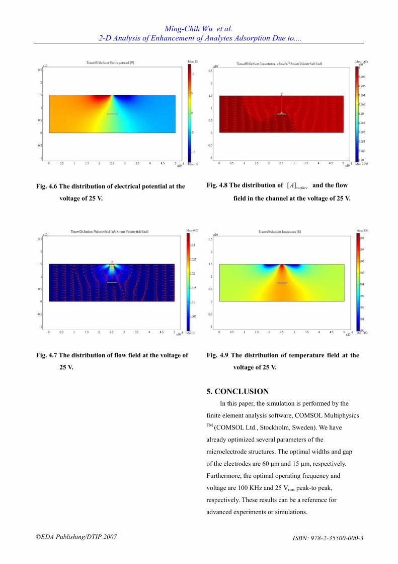
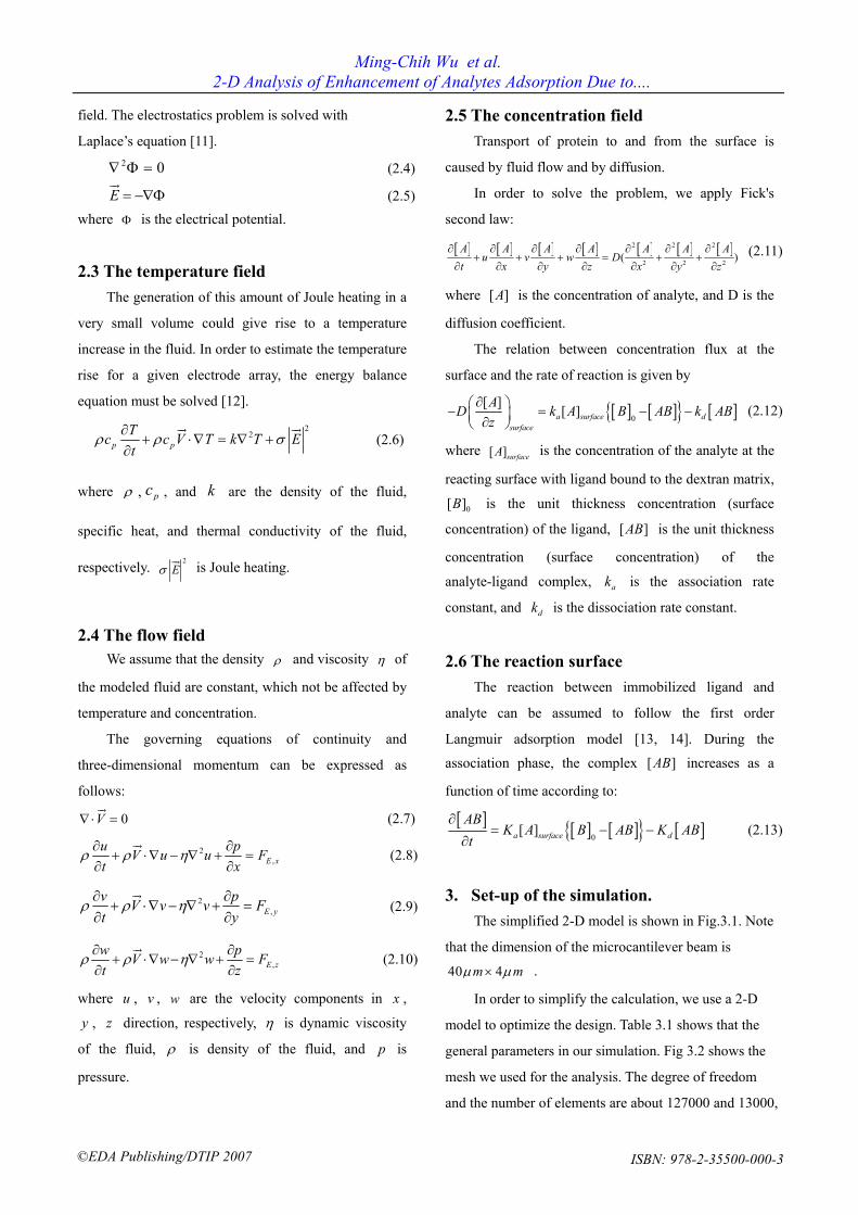
Fig. 4.6 The distribution of electrical potential at the
voltage of 25 V.
Fig. 4.7 The distribution of flow field at the voltage of
25 V.
Fig. 4.8 The distribution of [ ]surfaceA and the flow
field in the channel at the voltage of 25 V.
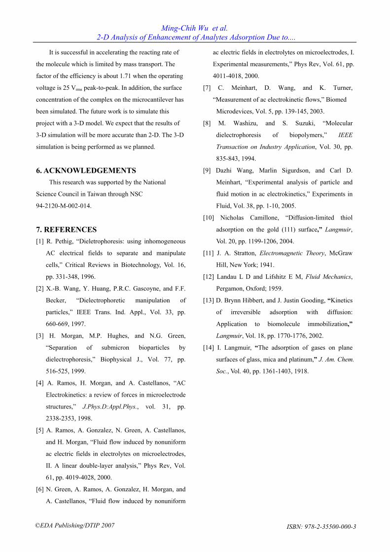
Fig. 4.9 The distribution of temperature field at the
voltage of 25 V.
5. CONCLUSION In this paper, the simulation is performed by the
finite element analysis software, COMSOL Multiphysics
TM (COMSOL Ltd., Stockholm, Sweden). We have
already optimized several parameters of the
microelectrode structures. The optimal widths and gap
of the electrodes are 60 μm and 15 μm, respectively.
Furthermore, the optimal operating frequency and
voltage are 100 KHz and 25 Vrms peak-to peak,
respectively. These results can be a reference for
advanced experiments or simulations.
Ming-Chih Wu et al.2-D Analysis of Enhancement of Analytes Adsorption Due to....
©EDA Publishing/DTIP 2007 ISBN: 978-2-35500-000-3
It is successful in accelerating the reacting rate of
the molecule which is limited by mass transport. The
factor of the efficiency is about 1.71 when the operating
voltage is 25 Vrms peak-to-peak. In addition, the surface
concentration of the complex on the microcantilever has
been simulated. The future work is to simulate this
project with a 3-D model. We expect that the results of
3-D simulation will be more accurate than 2-D. The 3-D
simulation is being performed as we planned.
6. ACKNOWLEDGEMENTS This research was supported by the National
Science Council in Taiwan through NSC
94-2120-M-002-014.
7. REFERENCES [1] R. Pethig, “Dieletrophoresis: using inhomogeneous
AC electrical fields to separate and manipulate
cells,” Critical Reviews in Biotechnology, Vol. 16,
pp. 331-348, 1996.
[2] X.-B. Wang, Y. Huang, P.R.C. Gascoyne, and F.F.
Becker, “Dielectrophoretic manipulation of
particles,” IEEE Trans. Ind. Appl., Vol. 33, pp.
660-669, 1997.
[3] H. Morgan, M.P. Hughes, and N.G. Green,
“Separation of submicron bioparticles by
dielectrophoresis,” Biophysical J., Vol. 77, pp.
516-525, 1999.
[4] A. Ramos, H. Morgan, and A. Castellanos, “AC
Electrokinetics: a review of forces in microelectrode
structures,” J.Phys.D:Appl.Phys., vol. 31, pp.
2338-2353, 1998.
[5] A. Ramos, A. Gonzalez, N. Green, A. Castellanos,
and H. Morgan, “Fluid flow induced by nonuniform
ac electric fields in electrolytes on microelectrodes,
II. A linear double-layer analysis,” Phys Rev, Vol.
61, pp. 4019-4028, 2000.
[6] N. Green, A. Ramos, A. Gonzalez, H. Morgan, and
A. Castellanos, “Fluid flow induced by nonuniform
ac electric fields in electrolytes on microelectrodes, I.
Experimental measurements,” Phys Rev, Vol. 61, pp.
4011-4018, 2000.
[7] C. Meinhart, D. Wang, and K. Turner,
“Measurement of ac electrokinetic flows,” Biomed
Microdevices, Vol. 5, pp. 139-145, 2003.
[8] M. Washizu, and S. Suzuki, “Molecular
dielectrophoresis of biopolymers,” IEEE
Transaction on Industry Application, Vol. 30, pp.
835-843, 1994. [9] Dazhi Wang, Marlin Sigurdson, and Carl D.
Meinhart, “Experimental analysis of particle and
fluid motion in ac electrokinetics,” Experiments in
Fluid, Vol. 38, pp. 1-10, 2005.
[10] Nicholas Camillone, “Diffusion-limited thiol
adsorption on the gold (111) surface,” Langmuir,
Vol. 20, pp. 1199-1206, 2004.
[11] J. A. Stratton, Electromagnetic Theory, McGraw
Hill, New York; 1941.
[12] Landau L D and Lifshitz E M, Fluid Mechanics,
Pergamon, Oxford; 1959.
[13] D. Brynn Hibbert, and J. Justin Gooding, “Kinetics
of irreversible adsorption with diffusion:
Application to biomolecule immobilization,”
Langmuir, Vol. 18, pp. 1770-1776, 2002.
[14] I. Langmuir, “The adsorption of gases on plane
surfaces of glass, mica and platinum,” J. Am. Chem.
Soc., Vol. 40, pp. 1361-1403, 1918.
Ming-Chih Wu et al.2-D Analysis of Enhancement of Analytes Adsorption Due to....
©EDA Publishing/DTIP 2007 ISBN: 978-2-35500-000-3
Top Related