


Languages
Pages
Legal

18-551, Spring 2003 Group 14, Final Report
Do What I Say!
Image Editing using Voice Commands
Chongseok (Alex) Park (park8) Trevor Tse (ttse)
Ka-Loon Tung (ktung)
18-551 Spring 2003 Group 14 - 1 -
Table of Contents Introduction: ............................................................................................... 2
Project Overview ......................................................................................... 3
Transfer Methods........................................................................................ 4
Prior 18-551 Relevant Works...................................................................... 5
Speech Recognition Algorithm ................................................................... 6
Decision Making Process ...........................................................................................6
Dynamic Time Warping..............................................................................................7 Coding Dynamic Time Warping .................................................................................9
Different Algorithms Attempted But Not Used .........................................................11
Image Processing Algorithm......................................................................12
Sharpen and Blur .....................................................................................................12 Pixelate.....................................................................................................................13
Brighten....................................................................................................................13 Grayscale ..................................................................................................................14
Rotate........................................................................................................................14 Undo .........................................................................................................................14
Memory Allocation.....................................................................................16
Speech Processing ....................................................................................................16 Image Processing .....................................................................................................16
Memory on the EVM ................................................................................................17
Speed Issues ...............................................................................................18
What We Did ............................................................................................................18
What We Tried..........................................................................................................19 What We Did Not Do................................................................................................20
EVM Profiling ...........................................................................................21
Demo and Tests..........................................................................................23
References..................................................................................................25
18-551 Spring 2003 Group 14 - 2 -
Introduction: Problem
Today, digital images are a new standard by which society can distribute
photographs. Innumerable digital images are exchanged among family and friends every
day via email and web pages. Thanks to the internet�s ability to transport these images
instantaneously, more and more people have begun using image-processing applications
to �clean up� their pictures before distributing. However, the majority of the existing
image processing applications, such as Adobe Photoshop, Paint Shop Pro, etc. contain
complex menus that intimidate inexperienced users. Many of these users do not have the
time to devote hours to learn all the menus/commands let alone master them in order to
filter pictures to achieve their desired results.
Solution
Our project is to implement an image processing application that can alleviate the
need for complicated menus, and provide the capabilities of the most commonly used
image-processing filters. The means of controlling these filters will be a voice input
through a microphone. From there, the TI C67 EVM will retrieve the voice input through
its MIC-in codec, and process it to determine what command was spoken. Then it will
run the image processing filter, and save it to a file that can be viewed by the user. We
will also feature an undo command for cases where there is an execution of the wrong
command, or if the user does not like the result.
18-551 Spring 2003 Group 14 - 3 -
Project Overview
The C program is first executed on to the PC side using Microsoft Visual C++.
Then it asks the user to input the filename of an image and the filename to store the
output (both in Portable Pix Map (PPM) format). Afterwards, the program is executed on
the EVM side using Code Composer Studio. The PC sends the picture to the TI C67
EVM (using HPI DMA transfer). Then, the user inputs a voice command through the
microphone via the CODEC on the TI C67 EVM. The speech is recorded at a sampling
rate of 5512 samples per second. The TI C67 EVM then sends the buffer containing the
speech to the PC using asynchronous PCI transfer. (In order to capture all of our speech
we made our buffer size 8000.) Afterwards, the PC down-samples and locates the main
part of the speech to lower the amount of samples. If there are too many samples (more
than 2000), the program will request the user re-enter his/her voice command. (This was
an effective way of getting rid of unwanted noise that was excessively high at the ends.)
Dynamic Time Warping (DTW) is then performed on the PC side to determine the match
possibility. The results of each DTW match possibility is then normalized by dividing
each value by the peak value of the magnitudes. Finally, these normalized values are
summed. The best match determined by this normalized sum is then sent back to the TI
C67 EVM (using a PCI synchronous message send), where the image is passed through
the best match image processing filter. The edited image is then sent back to the PC
using HPI DMA transfer and written to the output file.
18-551 Spring 2003 Group 14 - 4 -
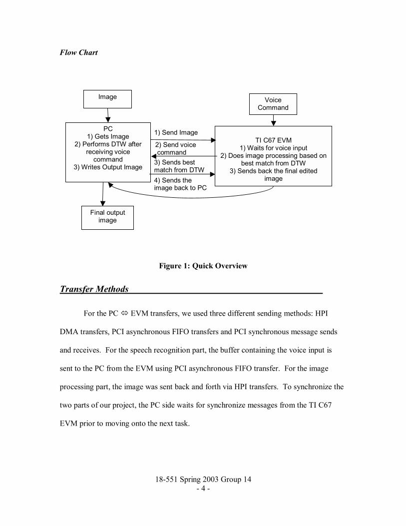
Flow Chart
Figure 1: Quick Overview
Transfer Methods
For the PC ! EVM transfers, we used three different sending methods: HPI
DMA transfers, PCI asynchronous FIFO transfers and PCI synchronous message sends
and receives. For the speech recognition part, the buffer containing the voice input is
sent to the PC from the EVM using PCI asynchronous FIFO transfer. For the image
processing part, the image was sent back and forth via HPI transfers. To synchronize the
two parts of our project, the PC side waits for synchronize messages from the TI C67
EVM prior to moving onto the next task.
Image
PC 1) Gets Image
2) Performs DTW after receiving voice
command 3) Writes Output Image
TI C67 EVM
1) Waits for voice input 2) Does image processing based on
best match from DTW 3) Sends back the final edited
image
1) Send Image
Voice Command
2) Send voice command3) Sends best match from DTW4) Sends the image back to PC
Final output image
18-551 Spring 2003 Group 14 - 5 -
Prior 18-551 Relevant Works
There were several previous 18-551 groups that dealt with speech recognition.
The following were used as references for our project.
Spring 1998, Group 13 � Voice Recognition for Embedded Systems
This project involved speech recognition for operating various household objects. The
voice command library contained about 15 small discrete words. This group used a
template based training set and made the speech recognition speaker dependent. This
project used dynamic time warping for speech recognition.
http://www.ece.cmu.edu/~ee551/Old_projects/projects/s_98_13/powerpointhtml/final/
Spring 1999, Group 18 � Text Independent Voice Transformation
This group dealt with speech recognition and voice transformation. They used linear
predictive coding with pitch detection to achieve speech recognition and voice
transformation.
http://www.ece.cmu.edu/~ee551/Old_projects/projects/s99_18/final.html
Spring 2000, Group 11 � Voice Recognition and Identification System
This group did a speech recognition project for identification of users. The library for
this project was small since it was only a password. This project also used dynamic time
warping for speech recognition.
http://www.ece.cmu.edu/~ee551/Final_Reports/Gr11.551.S00.pdf
18-551 Spring 2003 Group 14 - 6 -
Speech Recognition Algorithm
Decision Making Process
Although our speech recognition part used the Dynamic Time Warping (DTW)
algorithm instead of the Hidden Markov Model (HMM) algorithm, we still needed a
relatively large trained library. When we initially started researching speech recognition
algorithms, we came to an erroneous conclusion: we believed that the HMM algorithm
would be the ideal solution for our program.
Just about every webpage we visited showed that the HMM algorithm is one of
the most powerful speech recognition tools to date. Some websites even seemed to
indicate that HMM is just a more advanced version of DTW. Furthermore, Carnegie
Mellon University has its very own SPHINX (well known throughout the speech
recognition world) that uses a modified HMM algorithm to drive their speech recognition
program. After giving our preliminary presentation, we learned that the HMM algorithm
was indeed very suitable tool for speech recognition; however, HMM is used for robust
big vocabulary speech recognition, whereas our project focused on isolated, small
vocabulary speech recognition.
Our program only required seven words and they were spoken one at a time,
which fit the bill for DTW. The difference between HMM and DTW was the amount of
training each algorithm required to successfully perform speech recognition.
18-551 Spring 2003 Group 14 - 7 -
Dynamic Time Warping
The Dynamic Time Warping algorithm receives it�s named from the fact that it
compensates for the varying speeds and times of the spoken speech. The biggest problem
in speech recognition is not the difference in volume or frequency of the speaker�s voice
but rather the timing of the speech. DTW is an algorithm that takes care of that problem.
In essence, DTW makes �sspeeech� or �spech,� seem the same as �speech.� This is done
by a process that consists of matching the incoming speech with stored templates. The
template with the lowest distance measure from the input pattern is the recognized word.
The best match (lowest distance measure) is based upon dynamic programming. In order
to get the lowest distance measure, the distance measure between two feature vectors is
calculated using the Euclidean distance metric.
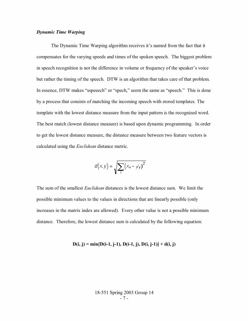
The sum of the smallest Euclidean distances is the lowest distance sum. We limit the
possible minimum values to the values in directions that are linearly possible (only
increases in the matrix index are allowed). Every other value is not a possible minimum
distance. Therefore, the lowest distance sum is calculated by the following equation:
D(i, j) = min[D(i-1, j-1), D(i-1, j), D(i, j-1)] + d(i, j)
18-551 Spring 2003 Group 14 - 8 -
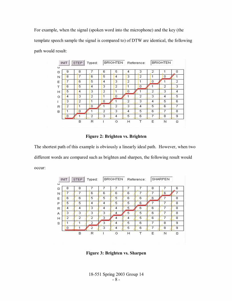
For example, when the signal (spoken word into the microphone) and the key (the
template speech sample the signal is compared to) of DTW are identical, the following
path would result:
Figure 2: Brighten vs. Brighten
The shortest path of this example is obviously a linearly ideal path. However, when two
different words are compared such as brighten and sharpen, the following result would
occur:
Figure 3: Brighten vs. Sharpen
18-551 Spring 2003 Group 14 - 9 -
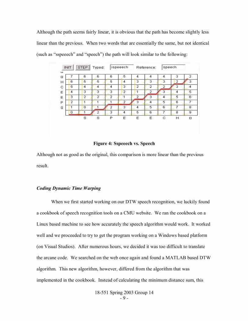
Although the path seems fairly linear, it is obvious that the path has become slightly less
linear than the previous. When two words that are essentially the same, but not identical
(such as �sspeeech� and �speech�) the path will look similar to the following:
Figure 4: Sspeeech vs. Speech
Although not as good as the original, this comparison is more linear than the previous
result.
Coding Dynamic Time Warping
When we first started working on our DTW speech recognition, we luckily found
a cookbook of speech recognition tools on a CMU website. We ran the cookbook on a
Linux based machine to see how accurately the speech algorithm would work. It worked
well and we proceeded to try to get the program working on a Windows based platform
(on Visual Studios). After numerous hours, we decided it was too difficult to translate
the arcane code. We searched on the web once again and found a MATLAB based DTW
algorithm. This new algorithm, however, differed from the algorithm that was
implemented in the cookbook. Instead of calculating the minimum distance sum, this
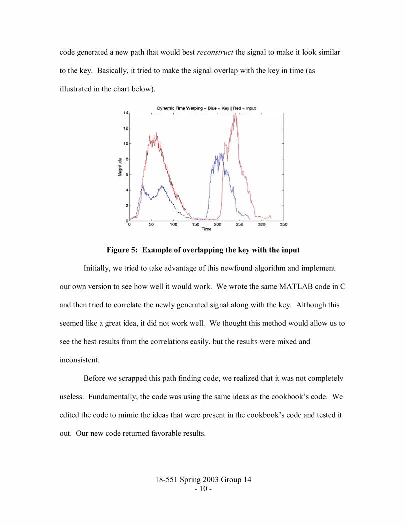
18-551 Spring 2003 Group 14 - 10 -
code generated a new path that would best reconstruct the signal to make it look similar
to the key. Basically, it tried to make the signal overlap with the key in time (as
illustrated in the chart below).
Figure 5: Example of overlapping the key with the input
Initially, we tried to take advantage of this newfound algorithm and implement
our own version to see how well it would work. We wrote the same MATLAB code in C
and then tried to correlate the newly generated signal along with the key. Although this
seemed like a great idea, it did not work well. We thought this method would allow us to
see the best results from the correlations easily, but the results were mixed and
inconsistent.
Before we scrapped this path finding code, we realized that it was not completely
useless. Fundamentally, the code was using the same ideas as the cookbook�s code. We
edited the code to mimic the ideas that were present in the cookbook�s code and tested it
out. Our new code returned favorable results.
18-551 Spring 2003 Group 14 - 11 -
Different Algorithms Attempted But Not Used
As mentioned before, we tried using the code we obtained to get the best path and
regenerate a new path for the signal that would best match the key in time. Then we tried
to correlate this new signal with the key and see which one would return the best result.
This method did not work as planned with inconsistent results.
Another idea we tried utilized our current DTW algorithm but tried to improve on
it. Because our DTW algorithm was too slow on the TI C67 EVM and even on the PC
side we tried to speed it up. In addition, we tried to improve our accuracy. Going
through previous years� projects and searching on the web, we found out that Linear
Predictive Coding (LPC) was an algorithm that aided speech recognition. LPC extracts
the most important parts in speech and uses those for speech recognition instead of the
actual whole speech.
LPC required an autocorrelation of the signal (speech we speak in to the microphone) and
then a new signal was made that had only the essential parts of the speech. Then we tried
using DTW on that new speech with the keys. This method worked to some extent and it
did yield extremely fast results. It was fast enough that we could have put it on the EVM.
(Basically, using LPC got rid our 2000x2000 size matrices and replaced them with 13x13
matrices). However, this method did not yield an improvement in accuracy of speech but
rather showed a decrement in the accuracy. We preferred accuracy to speed and decided
not to use this approach.

18-551 Spring 2003 Group 14 - 12 -
Image Processing Algorithm
The image processing filters that we implemented, sharpen, blur, pixelate,
grayscale, brighten, and rotate, all use relatively different operations to change the pixel
values within the image. Our project reads in a Portable Pix Map (PPM) format image,
using source code obtained from the teacher�s assistants. Once the header is decoded,
and the size of the image extracted, the contents of the image is read into an array of
bytes of size length*width*3 unsigned characters.
Sharpen and Blur
Sharpen and blur in essence use the same principles by which to edit the image.
When you sharpen an image, you want to decrease the influence neighboring pixels have
on the current pixel. In contrast, when you blur an image, you want to increase the
influence neighboring pixels have on the current pixel. Each pixel is convoluted with a
general 3x3 sharpening and blurring matrix and the result was summed and placed in the
corresponding location in the resulting image array. Because the values are stored in
bytes, the issue of overstepping the 255-value limit became an issue. As a result, we
altered each matrix so that it does not overstep the boundary.
Sharpen Matrix: Blurring Matrix: 0 -0.25 0 1/5 1/5 1/5
-0.25 2 -0.25 1/5 1/5 1/5 0 -0.25 0 1/5 1/5 1/5
Sharpen and Blur Matrices
18-551 Spring 2003 Group 14 - 13 -
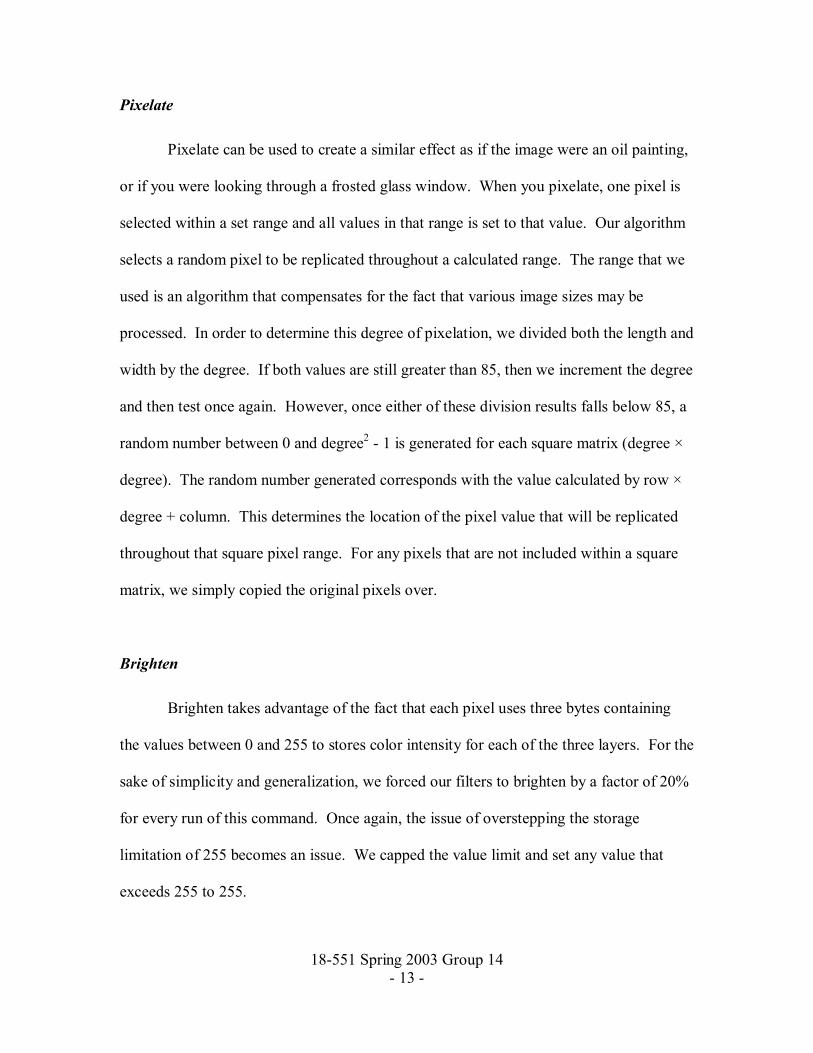
Pixelate
Pixelate can be used to create a similar effect as if the image were an oil painting,
or if you were looking through a frosted glass window. When you pixelate, one pixel is
selected within a set range and all values in that range is set to that value. Our algorithm
selects a random pixel to be replicated throughout a calculated range. The range that we
used is an algorithm that compensates for the fact that various image sizes may be
processed. In order to determine this degree of pixelation, we divided both the length and
width by the degree. If both values are still greater than 85, then we increment the degree
and then test once again. However, once either of these division results falls below 85, a
random number between 0 and degree2 - 1 is generated for each square matrix (degree ×
degree). The random number generated corresponds with the value calculated by row ×
degree + column. This determines the location of the pixel value that will be replicated
throughout that square pixel range. For any pixels that are not included within a square
matrix, we simply copied the original pixels over.
Brighten
Brighten takes advantage of the fact that each pixel uses three bytes containing
the values between 0 and 255 to stores color intensity for each of the three layers. For the
sake of simplicity and generalization, we forced our filters to brighten by a factor of 20%
for every run of this command. Once again, the issue of overstepping the storage
limitation of 255 becomes an issue. We capped the value limit and set any value that
exceeds 255 to 255.
18-551 Spring 2003 Group 14 - 14 -
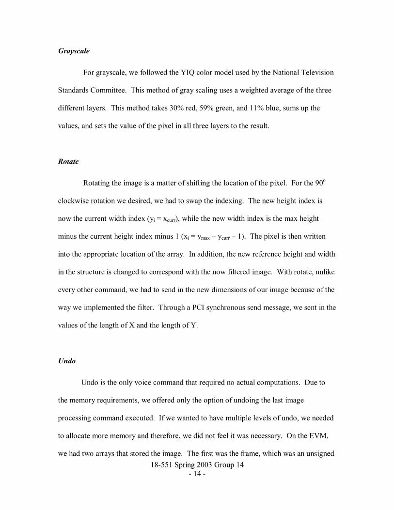
Grayscale
For grayscale, we followed the YIQ color model used by the National Television
Standards Committee. This method of gray scaling uses a weighted average of the three
different layers. This method takes 30% red, 59% green, and 11% blue, sums up the
values, and sets the value of the pixel in all three layers to the result.
Rotate
Rotating the image is a matter of shifting the location of the pixel. For the 90o
clockwise rotation we desired, we had to swap the indexing. The new height index is
now the current width index (yi = xcurr), while the new width index is the max height
minus the current height index minus 1 (xi = ymax � ycurr � 1). The pixel is then written
into the appropriate location of the array. In addition, the new reference height and width
in the structure is changed to correspond with the now filtered image. With rotate, unlike
every other command, we had to send in the new dimensions of our image because of the
way we implemented the filter. Through a PCI synchronous send message, we sent in the
values of the length of X and the length of Y.
Undo
Undo is the only voice command that required no actual computations. Due to
the memory requirements, we offered only the option of undoing the last image
processing command executed. If we wanted to have multiple levels of undo, we needed
to allocate more memory and therefore, we did not feel it was necessary. On the EVM,
we had two arrays that stored the image. The first was the frame, which was an unsigned
18-551 Spring 2003 Group 14 - 15 -
character array, and the second was result. Working with these two arrays, we simply
copied the result back into frame right before each image processing command is to be
executed. If �undo� is the recognized speech input from the microphone, the frame is
copied into result (over-writing the previous result). This process undoes the last image
processing command that is executed.
18-551 Spring 2003 Group 14 - 16 -
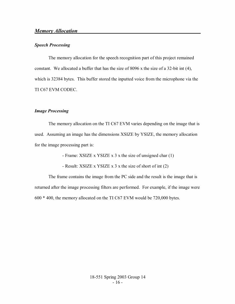
Memory Allocation
Speech Processing
The memory allocation for the speech recognition part of this project remained
constant. We allocated a buffer that has the size of 8096 x the size of a 32-bit int (4),
which is 32384 bytes. This buffer stored the inputted voice from the microphone via the
TI C67 EVM CODEC.
Image Processing
The memory allocation on the TI C67 EVM varies depending on the image that is
used. Assuming an image has the dimensions XSIZE by YSIZE, the memory allocation
for the image processing part is:
- Frame: XSIZE x YSIZE x 3 x the size of unsigned char (1)
- Result: XSIZE x YSIZE x 3 x the size of short of int (2)
The frame contains the image from the PC side and the result is the image that is
returned after the image processing filters are performed. For example, if the image were
600 * 400, the memory allocated on the TI C67 EVM would be 720,000 bytes.
18-551 Spring 2003 Group 14 - 17 -
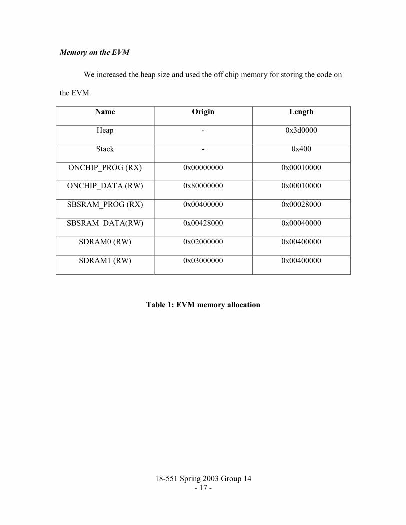
Memory on the EVM
We increased the heap size and used the off chip memory for storing the code on
the EVM.
Name Origin Length
Heap - 0x3d0000
Stack - 0x400
ONCHIP_PROG (RX) 0x00000000 0x00010000
ONCHIP_DATA (RW) 0x80000000 0x00010000
SBSRAM_PROG (RX) 0x00400000 0x00028000
SBSRAM_DATA(RW) 0x00428000 0x00040000
SDRAM0 (RW) 0x02000000 0x00400000
SDRAM1 (RW) 0x03000000 0x00400000
Table 1: EVM memory allocation
18-551 Spring 2003 Group 14 - 18 -
Speed Issues
What We Did
When we first got the speech recognition DTW algorithm working, the
calculations took an excessive amount of time to complete. In order to speed up the
algorithm, we attempted to remove as many double for loop calculations as possible. The
initialization of the local distance matrix (LDM) and the accumulative distance matrix
(ADM) were the first loops removed. Since we calculated the LDM in the next double
for loop, and every value was calculated and set in that loop, we were able to remove
initialization of the LDM. Also by shifting the ADM initialization into the LDM
calculation loop, we were able to remove yet another loop. In addition, we removed a
third double for loop when calculating the �best choice� for the next step in our
algorithm. The result was a decrease of approximately 60% of the time required, since
we removed three of the five double for loops. These double for loops wouldn�t have
been a problem if they were simply in their teens, but these loops continued on into
ranges greater than that of 4000. Memory wise, this code did not work on the EVM
because the EVM�s maximum memory is approximately 8 megabytes. We had to find a
way through this problem because we required the big matrices to be there.
The result of this optimization was still inadequate to improve the overall
performance of our algorithm. We realized that our DTW required only key points to
perform the accuracy check. First, we cut off the noise that was sent into our algorithm
but cutting off values that did not exceed a normalized threshold value of 0.2. This
removed the noise, and cut down length of the sample from 8096 to less than 4000
samples. Afterwards, we down sampled by a factor of two. The resulting performance

18-551 Spring 2003 Group 14 - 19 -
was much faster than the initial algorithm, with an indistinguishable difference in
accuracy rate. Performance overall was acceptable for individual runs of the algorithm.
After performing all these optimizations, we were able to run the DTW code on the
EVM. However, because of the number of trained values (42), and the difference in
speed of the PC�s processor of 1.8 GHz and the EVM�s speed of 167MHz, the overall
time requirement when processing on the EVM was unrealistically long. We had no
choice but to leave the speech processing on the PC side.
For the image processing, due to time constraints, we were unable to complete
any significant optimizations. Therefore, the only optimization that we implemented was
Code Composer�s built in loop unrolling feature. The result was a slight increase in
speed for the image processing filters.
What We Tried
Our further attempts to improve the speed of our DTW algorithm was first to
employ LPC (Linear Predictive Coding). LPC is a method of down sampling that
extracts the key parts of the input waveform. These key parts are also the changes in the
tones of the input waveform. The result is a list of coefficients for a filter that will
reproduce a similar waveform. However, the result of our LPC calculations was rejected
because of the decrease in accuracy. Though it improved the improved the speed of our
algorithm dramatically, the resulting accuracy rate dropped from roughly 75%-80%, to
10%-15%. We decided to reject any further attempts of programming this algorithm due
to time constraints.
18-551 Spring 2003 Group 14 - 20 -
What We Did Not Do
Because the DTW algorithm caused the brunt of our speed issues, we attempted to
optimize it as much as possible and import it to the EVM. However all working
optimizations still resulted in an unacceptable speed when testing on the EVM.
Due to time constraints, we did not have enough time to optimize the image-
processing filters. However, ideas for optimization that we were ready to employ are
paging and parallelization. In filters such as grayscale and brighten, paging would not be
hard to accomplish, since it processing each pixel individually and completes all
processing before moving onto the next. Sharpen, blur, and pixelate would be more
complicated, and will require a larger segment of input data to be paged compared to the
output. Rotate is the only function that would provide an issue in paging, since it takes
segments and reroutes the index.

18-551 Spring 2003 Group 14 - 21 -
EVM Profiling
The TI C67 EVM allows profiling of specific functions that are placed on the
board.
Image Processing Filter (Big O notation) Number of Cycles on the EVM
Brighten O(n) 43,217,781
Sharpen O(n2) 176,238,856
Blur O(n2) 176,538,645
Gray Scale O(n) 27,885,808
Pixelate O(n4) 331,429,540
Rotate O(n) 29,020,405
Table 2: Profiling of functions on the EVM
For some reason, these values were greater than that of what we expected. We based our
image processing codes on lab 3 and therefore most of the results should have yielded
similar results. However, our results were significantly greater. The only possible
reasons for this discrepancy can be the computer we profiled on (or the EVM) was
somehow problematic or the way we carried out our filters were somehow worse than the
edge detection filter we did in lab 3. Although our sharpen algorithm and edge detection
filter basically perform the same task, we wrote it differently because we tested and
coded our own filters.
18-551 Spring 2003 Group 14 - 22 -
Training and Test Sets
Training was a critical part of our speech recognition program. Although DTW is
an algorithm that is really highlighted for its ability to work with minimal training, the
more we increased the number of training samples, the better our speech recognition
accuracy got. Initially, we tested our algorithm with only one set of templates. We
recorded Alex�s voice through a microphone connected to the EVM through the CODEC
and using our own data format, recorded the speech onto a file. We needed seven
samples because we needed a sample for each image processing command (brighten,
sharpen, pixelate, rotate, blur, grayscale), and another for undo.
When we tested the accuracy in matching what was spoken with one reference
template, the accuracy was acceptable when Alex tested the algorithm (~70% accuracy),
but it was much lower when Ka-Loon and Trevor tested it (~45% accuracy). Then we
tried two sets of templates that Alex recorded again. As expected, the accuracy rose for
Alex (~75%), but it was a surprise that it rose for other people as well (~50%).
Ultimately we decided on using two sets for each individual in our group, which resulted
in six sets of training data. This gave the best balance in accuracy and speaker
independence (at least among the three of us). For our final results, we wound up with
~76% accuracy.
For our image processing part, we did not require any training. Our image
processing was filters, some that were similar to the edge detection filter that we did in
lab 3. However, we did have to go through testing in MATLAB to see how well our
filters worked and tweaked it to our tastes.
18-551 Spring 2003 Group 14 - 23 -
Demo and Tests
Demo
For our demo, we load an image (300 x 197 or 600 x 400) onto the TI C67 EVM
through our user interface by typing in the filename of the image. (We did not test any
other sizes but we presume they would work as well.) We then say any one of the seven
commands and show the output of the performed image processing filters.
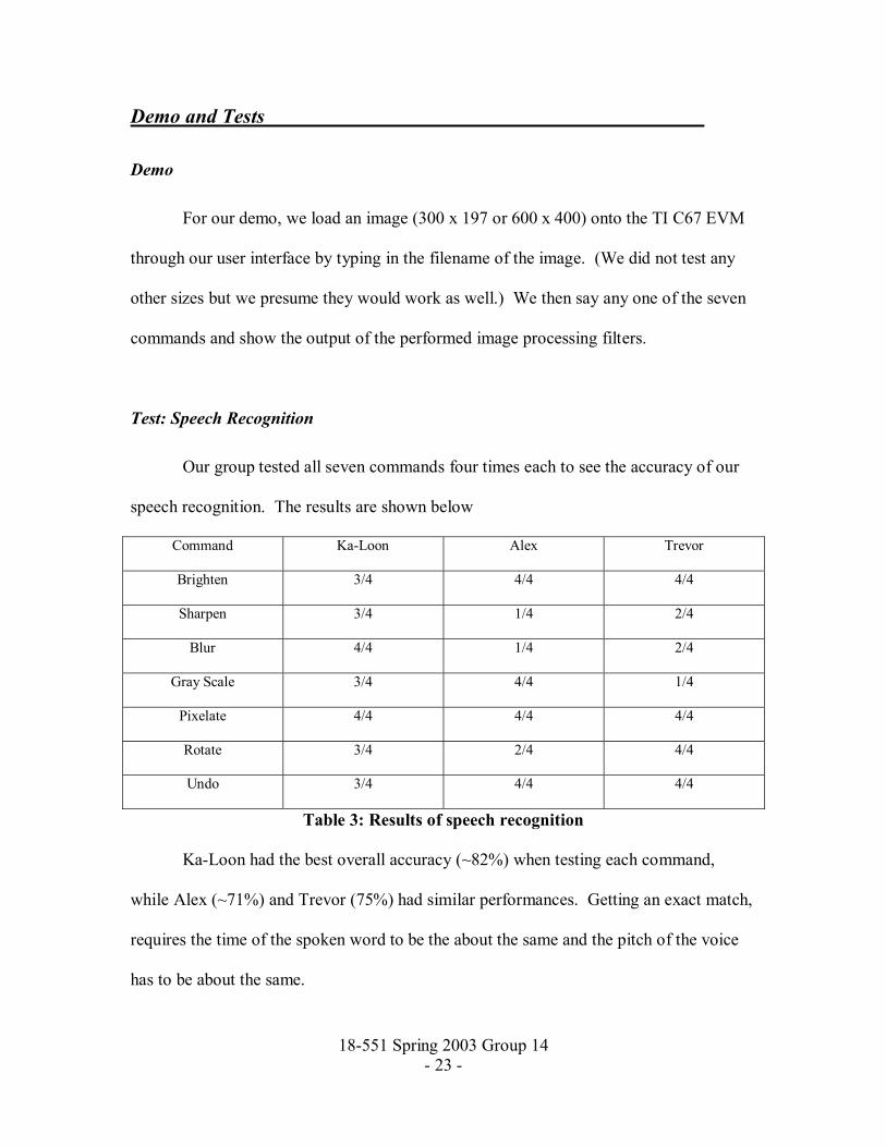
Test: Speech Recognition
Our group tested all seven commands four times each to see the accuracy of our
speech recognition. The results are shown below
Command Ka-Loon Alex Trevor
Brighten 3/4 4/4 4/4
Sharpen 3/4 1/4 2/4
Blur 4/4 1/4 2/4
Gray Scale 3/4 4/4 1/4
Pixelate 4/4 4/4 4/4
Rotate 3/4 2/4 4/4
Undo 3/4 4/4 4/4
Table 3: Results of speech recognition
Ka-Loon had the best overall accuracy (~82%) when testing each command,
while Alex (~71%) and Trevor (75%) had similar performances. Getting an exact match,
requires the time of the spoken word to be the about the same and the pitch of the voice
has to be about the same.

18-551 Spring 2003 Group 14 - 24 -
Test: Image Processing
This is the inputted image that we tested on the EVM. The size of this picture is 300 x
197.
Figure 6: Original image
The following pictures were outputted from the TI C67 EVM to the PC.
Figure 7: Edited images outputted from the EVM
Brighten Sharpen Blur
Gray Pixelate Rotate
18-551 Spring 2003 Group 14 - 25 -
References
Speech Recognition
1) Dynamic Time Warping
http://www.cnel.ufl.edu/~kkale/dtw.html
2) Dynamic Time Warping
http://www.owlnet.rice.edu/~elec301/Projects99/wrcocee/imp.htm
3) Dynamic Time Warping
http://www-2.cs.cmu.edu/afs/cs/project/ai-
repository/ai/areas/speech/systems/cookbook/0.html
Image Processing
1) Digital Image Processing: concepts, Algorithms, and Applications by Bernd
Jahne. New York, New York: Springer-Verlag, ©1991
2) PPM Library (Received from TA�s)
Previous Groups
1) Spring 1998, Group 13
2) Spring 1999, Group 18
3) Spring 2000, Group 11
Figures
Figures 2-4
http://www.cnel.ufl.edu/~kkale/dtw.html
Figure 5
http://www.owlnet.rice.edu/~elec301/Projects99/wrcocee/imp.htm
Top Related