Download - 16.28 GROEBNER: A Gröbner basis package - Reducereduce-algebra.sourceforge.net/manual/contributed/groebner.pdf · 532 CHAPTER 16. USER CONTRIBUTED PACKAGES 16.28 GROEBNER: A Gröbner

532 CHAPTER 16. USER CONTRIBUTED PACKAGES

16.28 GROEBNER: A Gröbner basis package

GROEBNER is a package for the computation of Gröbner Bases using the Buch-berger algorithm and related methods for polynomial ideals and modules. It can beused over a variety of different coefficient domains, and for different variable andterm orderings.

Gröbner Bases can be used for various purposes in commutative algebra, e.g. forelimination of variables, converting surd expressions to implicit polynomial form,computation of dimensions, solution of polynomial equation systems etc. Thepackage is also used internally by the SOLVE operator.

Authors: Herbert Melenk, H.M. Möller and Winfried Neun.

Gröbner bases are a valuable tool for solving problems in connection with multi-variate polynomials, such as solving systems of algebraic equations and analyzingpolynomial ideals. For a definition of Gröbner bases, a survey of possible applica-tions and further references, see [6]. Examples are given in [5], in [7] and also inthe test file for this package.

The groebner package calculates Gröbner bases using the Buchberger algorithm.It can be used over a variety of different coefficient domains, and for differentvariable and term orderings.

The current version of the package uses parts of a previous version, written by R.Gebauer, A.C. Hearn, H. Kredel and H. M. Möller. The algorithms implementedin the current version are documented in [10], [11], [15] and [12]. The operatorsaturation has been implemented in July 2000 (Herbert Melenk).

16.28.1 Background

Variables, Domains and Polynomials

The various functions of the groebner package manipulate equations and/or poly-nomials; equations are internally transformed into polynomials by forming the dif-ference of left-hand side and right-hand side, if equations are given.

All manipulations take place in a ring of polynomials in some variables x1, . . . , xnover a coefficient domain d:

d[x1, . . . , xn],

where d is a field or at least a ring without zero divisors. The set of variablesx1, . . . , xn can be given explicitly by the user or it is extracted automatically fromthe input expressions.

All REDUCE kernels can play the role of “variables” in this context; examples are

533

x y z22 sin(alpha) cos(alpha) c(1,2,3) c(1,3,2) farina4711

The domain d is the current REDUCE domain with those kernels adjoined that arenot members of the list of variables. So the elements of d may be complicatedpolynomials themselves over kernels not in the list of variables; if, however, thevariables are extracted automatically from the input expressions, d is identical withthe current REDUCE domain. It is useful to regard kernels not being members ofthe list of variables as “parameters”, e.g.

a ∗ x+ (a− b) ∗ y ∗ ∗2 with “variables” {x, y}and “parameters” a and b .

The exponents of groebner variables must be positive integers.

A groebner variable may not occur as a parameter (or part of a parameter) ofa coefficient function. This condition is tested in the beginning of the groebnercalculation; if it is violated, an error message occurs (with the variable name), andthe calculation is aborted. When the groebner package is called by solve, the testis switched off internally.

The current version of the Buchberger algorithm has two internal modes, a fieldmode and a ring mode. In the starting phase the algorithm analyzes the domaintype; if it recognizes d as being a ring it uses the ring mode, otherwise the fieldmode is needed. Normally field calculations occur only if all coefficients are num-bers and if the current REDUCE domain is a field (e.g. rational numbers, modularnumbers modulo a prime). In general, the ring mode is faster. When no specificREDUCE domain is selected, the ring mode is used, even if the input formulascontain fractional coefficients: they are multiplied by their common denominatorsso that they become integer polynomials. Zeroes of the denominators are includedin the result list.

Term Ordering

In the theory of Gröbner bases, the terms of polynomials are considered as or-dered. Several order modes are available in the current package, including thebasic modes:

lex, gradlex, revgradlex

All orderings are based on an ordering among the variables. For each pair of vari-ables (a, b) an order relation must be defined, e.g. “a � b”. The greater sign�does not represent a numerical relation among the variables; it can be interpretedonly in terms of formula representation: “a” will be placed in front of “b” or “a” ismore complicated than “b”.


The sequence of variables constitutes this order base. So the notion of

{x1, x2, x3}

as a list of variables at the same time means

x1� x2� x3

with respect to the term order.

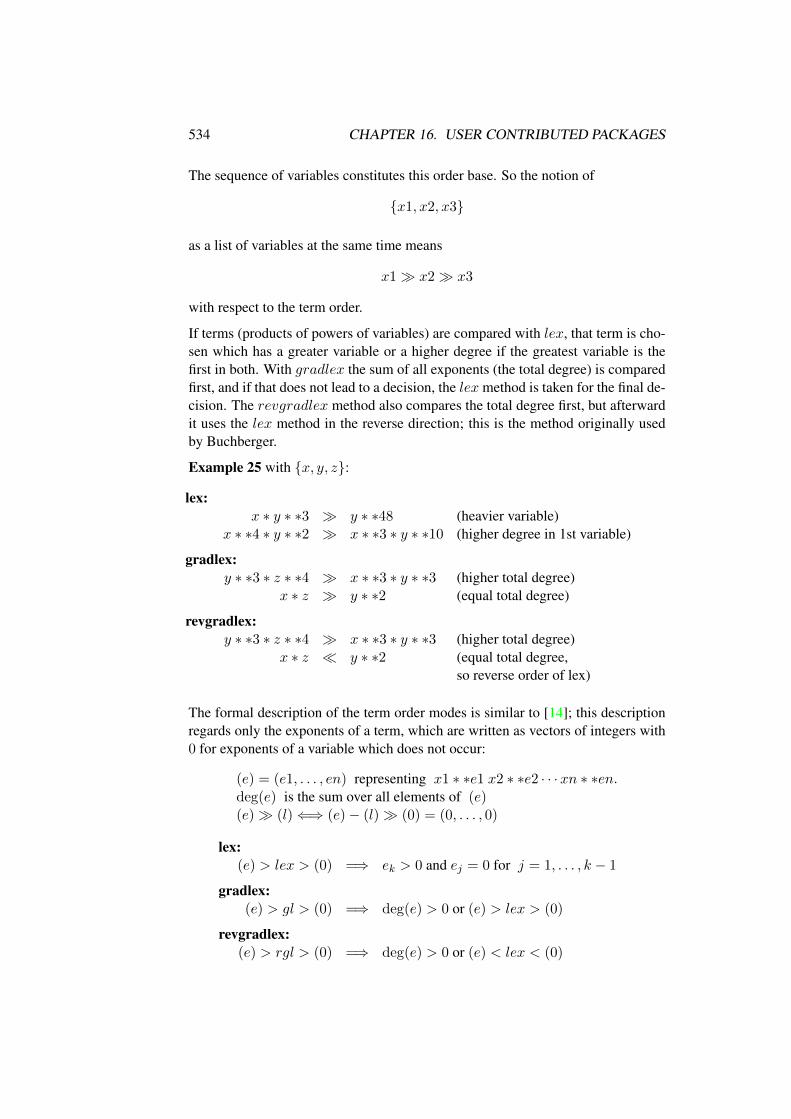
If terms (products of powers of variables) are compared with lex, that term is cho-sen which has a greater variable or a higher degree if the greatest variable is thefirst in both. With gradlex the sum of all exponents (the total degree) is comparedfirst, and if that does not lead to a decision, the lex method is taken for the final de-cision. The revgradlex method also compares the total degree first, but afterwardit uses the lex method in the reverse direction; this is the method originally usedby Buchberger.

Example 25 with {x, y, z}:

lex:x ∗ y ∗ ∗3 � y ∗ ∗48 (heavier variable)

x ∗ ∗4 ∗ y ∗ ∗2 � x ∗ ∗3 ∗ y ∗ ∗10 (higher degree in 1st variable)

gradlex:y ∗ ∗3 ∗ z ∗ ∗4 � x ∗ ∗3 ∗ y ∗ ∗3 (higher total degree)

x ∗ z � y ∗ ∗2 (equal total degree)

revgradlex:y ∗ ∗3 ∗ z ∗ ∗4 � x ∗ ∗3 ∗ y ∗ ∗3 (higher total degree)

x ∗ z � y ∗ ∗2 (equal total degree,so reverse order of lex)

The formal description of the term order modes is similar to [14]; this descriptionregards only the exponents of a term, which are written as vectors of integers with0 for exponents of a variable which does not occur:

(e) = (e1, . . . , en) representing x1 ∗ ∗e1 x2 ∗ ∗e2 · · ·xn ∗ ∗en.deg(e) is the sum over all elements of (e)(e)� (l)⇐⇒ (e)− (l)� (0) = (0, . . . , 0)

lex:(e) > lex > (0) =⇒ ek > 0 and ej = 0 for j = 1, . . . , k − 1

gradlex:(e) > gl > (0) =⇒ deg(e) > 0 or (e) > lex > (0)

revgradlex:(e) > rgl > (0) =⇒ deg(e) > 0 or (e) < lex < (0)

535

Note that the lex ordering is identical to the standard REDUCE kernel ordering,when korder is set explicitly to the sequence of variables.

lex is the default term order mode in the groebner package.

It is beyond the scope of this manual to discuss the functionality of the term ordermodes. See [7].

The list of variables is declared as an optional parameter of the torder statement(see below). If this declaration is missing or if the empty list has been used, thevariables are extracted from the expressions automatically and the REDUCE sys-tem order defines their sequence; this can be influenced by setting an explicit ordervia the korder statement.

The result of a Gröbner calculation is algebraically correct only with respect to theterm order mode and the variable sequence which was in effect during the calcu-lation. This is important if several calls to the groebner package are done withthe result of the first being the input of the second call. Therefore we recommendthat you declare the variable list and the order mode explicitly. Once declared it re-mains valid until you enter a new torder statement. The operator gvars helps youextract the variables from a given set of polynomials, if an automatic reorderinghas been selected.

The Buchberger Algorithm

The Buchberger algorithm of the package is based on GEBAUER/MÖLLER [11].Extensions are documented in [16] and [12].

16.28.2 Loading of the Package

The following command loads the package into REDUCE (this syntax may varyaccording to the implementation):

load_package groebner;

The package contains various operators, and switches for control over the reductionprocess. These are discussed in the following.

16.28.3 The Basic Operators

Term Ordering Mode

torder (vl,m,[p1, p2, . . .]);


where vl is a variable list (or the empty list if no variables are declared ex-plicitly), m is the name of a term ordering mode lex, gradlex, revgradlex(or another implemented mode) and [p1, p2, . . .] are additional parametersfor the term ordering mode (not needed for the basic modes).

torder sets variable set and the term ordering mode. The default mode is lex.The previous description is returned as a list with corresponding elements.Such a list can alternatively be passed as sole argument to torder.

If the variable list is empty or if the torder declaration is omitted, the auto-matic variable extraction is activated.

gvars ({exp1, exp2, . . ., expn});

where {exp1, exp2, . . . , expn} is a list of expressions or equations.

gvars extracts from the expressions {exp1, exp2, . . . , expn} the kernels,which can play the role of variables for a Gröbner calculation. This can beused e.g. in a torder declaration.

groebner: Calculation of a Gröbner Basis

groebner {exp1, exp2, . . . , expm};where {exp1, exp2, . . . , expm} is a list of expressions or equations.

groebner calculates the Gröbner basis of the given set of expressions withrespect to the current torder setting.

The Gröbner basis {1}means that the ideal generated by the input polynom-ials is the whole polynomial ring, or equivalently, that the input polynomialshave no zeroes in common.

As a side effect, the sequence of variables is stored as a REDUCE list in theshared variable

gvarslast.

This is important if the variables are reordered because of optimization: youmust set them afterwards explicitly as the current variable sequence if youwant to use the Gröbner basis in the sequel, e.g. for a preduce call. Abasis has the property “Gröbner” only with respect to the variable sequenceswhich had been active during its computation.

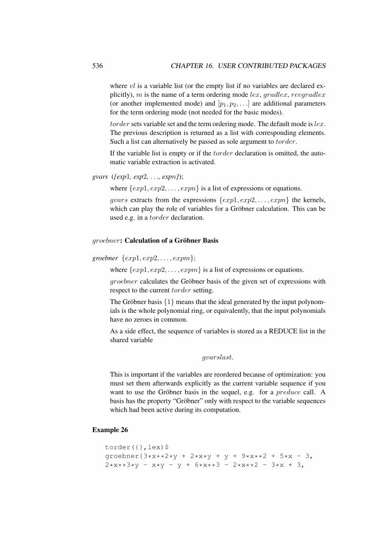
Example 26

torder({},lex)$groebner{3*x**2*y + 2*x*y + y + 9*x**2 + 5*x - 3,2*x**3*y - x*y - y + 6*x**3 - 2*x**2 - 3*x + 3,

537

x**3*y + x**2*y + 3*x**3 + 2*x**2 };

2{8*x - 2*y + 5*y + 3,

3 22*y - 3*y - 16*y + 21}

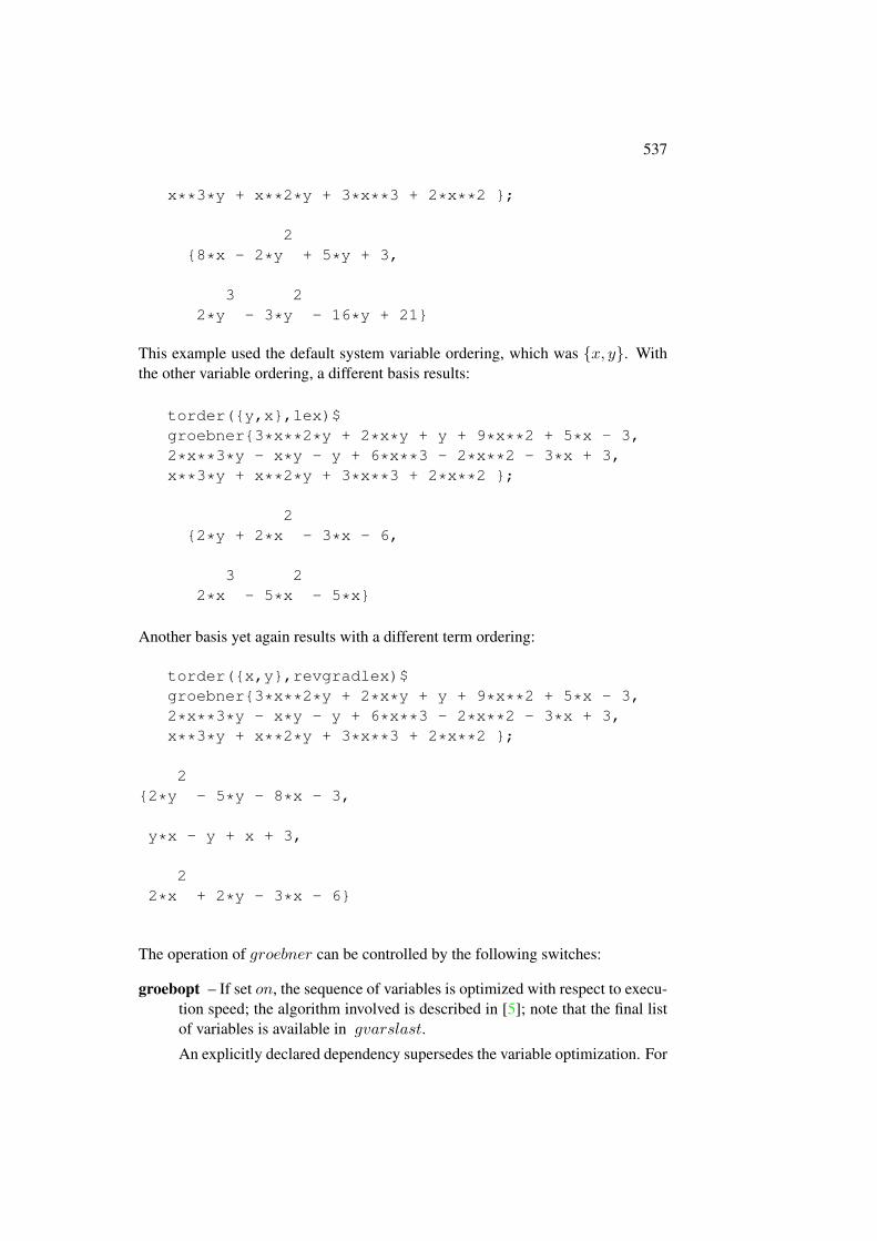
This example used the default system variable ordering, which was {x, y}. Withthe other variable ordering, a different basis results:

torder({y,x},lex)$groebner{3*x**2*y + 2*x*y + y + 9*x**2 + 5*x - 3,2*x**3*y - x*y - y + 6*x**3 - 2*x**2 - 3*x + 3,x**3*y + x**2*y + 3*x**3 + 2*x**2 };

2{2*y + 2*x - 3*x - 6,

3 22*x - 5*x - 5*x}

Another basis yet again results with a different term ordering:

torder({x,y},revgradlex)$groebner{3*x**2*y + 2*x*y + y + 9*x**2 + 5*x - 3,2*x**3*y - x*y - y + 6*x**3 - 2*x**2 - 3*x + 3,x**3*y + x**2*y + 3*x**3 + 2*x**2 };

2{2*y - 5*y - 8*x - 3,

y*x - y + x + 3,

22*x + 2*y - 3*x - 6}

The operation of groebner can be controlled by the following switches:

groebopt – If set on, the sequence of variables is optimized with respect to execu-tion speed; the algorithm involved is described in [5]; note that the final listof variables is available in gvarslast.

An explicitly declared dependency supersedes the variable optimization. For


example

depend a, x, y;

guarantees that a will be placed in front of x and y. So groebopt can be usedeven in cases where elimination of variables is desired.

By default groebopt is off , conserving the original variable sequence.

groebfullreduction – If set off , the reduction steps during thegroebner operation are limited to the pure head term reduction; subsequentterms are reduced otherwise.

By default groebfullreduction is on.

gltbasis – If set on, the leading terms of the result basis are extracted. They arecollected in a basis of monomials, which is available as value of the globalvariable with the name gltb.

glterms – If {exp1, . . . , expm} contain parameters (symbols which are not mem-ber of the variable list), the share variable glterms contains a list of expres-sion which during the calculation were assumed to be nonzero. A Gröbnerbasis is valid only under the assumption that all these expressions do notvanish.

The following switches control the print output of groebner; by default all theseswitches are set off and nothing is printed.

groebstat – A summary of the computation is printed including the computingtime, the number of intermediate h–polynomials and the counters for thehits of the criteria.

trgroeb – Includes groebstat and the printing of the intermediate h-polynomials.

trgroebs – Includes trgroeb and the printing of intermediate s–polynomials.

trgroeb1 – The internal pairlist is printed when modified.

Gzerodim?: Test of dim = 0

gzerodim!? baswhere bas is a Gröbner basis in the current setting. The result is nil, if bas isthe basis of an ideal of polynomials with more than finitely many commonzeros. If the ideal is zero dimensional, i. e. the polynomials of the ideal haveonly finitely many zeros in common, the result is an integer k which is thenumber of these common zeros (counted with multiplicities).

539

gdimension, gindependent_sets: compute dimension and independent vari-ables

The following operators can be used to compute the dimension and the independentvariable sets of an ideal which has the Gröbner basis bas with arbitrary term order:

gdimension bas

gindependent_sets bas gindependent_sets computes the maximal left indepen-dent variable sets of the ideal, that are the variable sets which play the roleof free parameters in the current ideal basis. Each set is a list which is asubset of the variable list. The result is a list of these sets. For an ideal withdimension zero the list is empty. gdimension computes the dimension of theideal, which is the maximum length of the independent sets.

The switch groebopt plays no role in the algorithms gdimension and gindependent_sets.It is set off during the processing even if it is set on before. Its state is saved duringthe processing.

The “Kredel-Weispfenning" algorithm is used (see [15], extended to general order-ing in [4].

Conversion of a Gröbner Basis

glexconvert: Conversion of an Arbitrary Gröbner Basis of a Zero Dimen-sional Ideal into a Lexical One

glexconvert ({exp, . . . , expm} [, {var1 . . . , varn}] [,maxdeg = mx][, newvars = {nv1, . . . , nvk}])where {exp1, . . . , expm} is a Gröbner basis with {var1, . . . , varn} as vari-ables in the current term order mode, mx is an integer, and {nv1, . . . , nvk}is a subset of the basis variables. For this operator the source and targetvariable sets must be specified explicitly.

glexconvert converts a basis of a zero-dimensional ideal (finite number of isolatedsolutions) from arbitrary ordering into a basis under lex ordering. During the callof glexconvert the original ordering of the input basis must be still active!

newvars defines the new variable sequence. If omitted, the original variable se-quence is used. If only a subset of variables is specified here, the partial ideal basisis evaluated. For the calculation of a univariate polynomial, newvars should be alist with one element.

maxdeg is an upper limit for the degrees. The algorithm stops with an error mes-sage, if this limit is reached.


A warning occurs if the ideal is not zero dimensional.

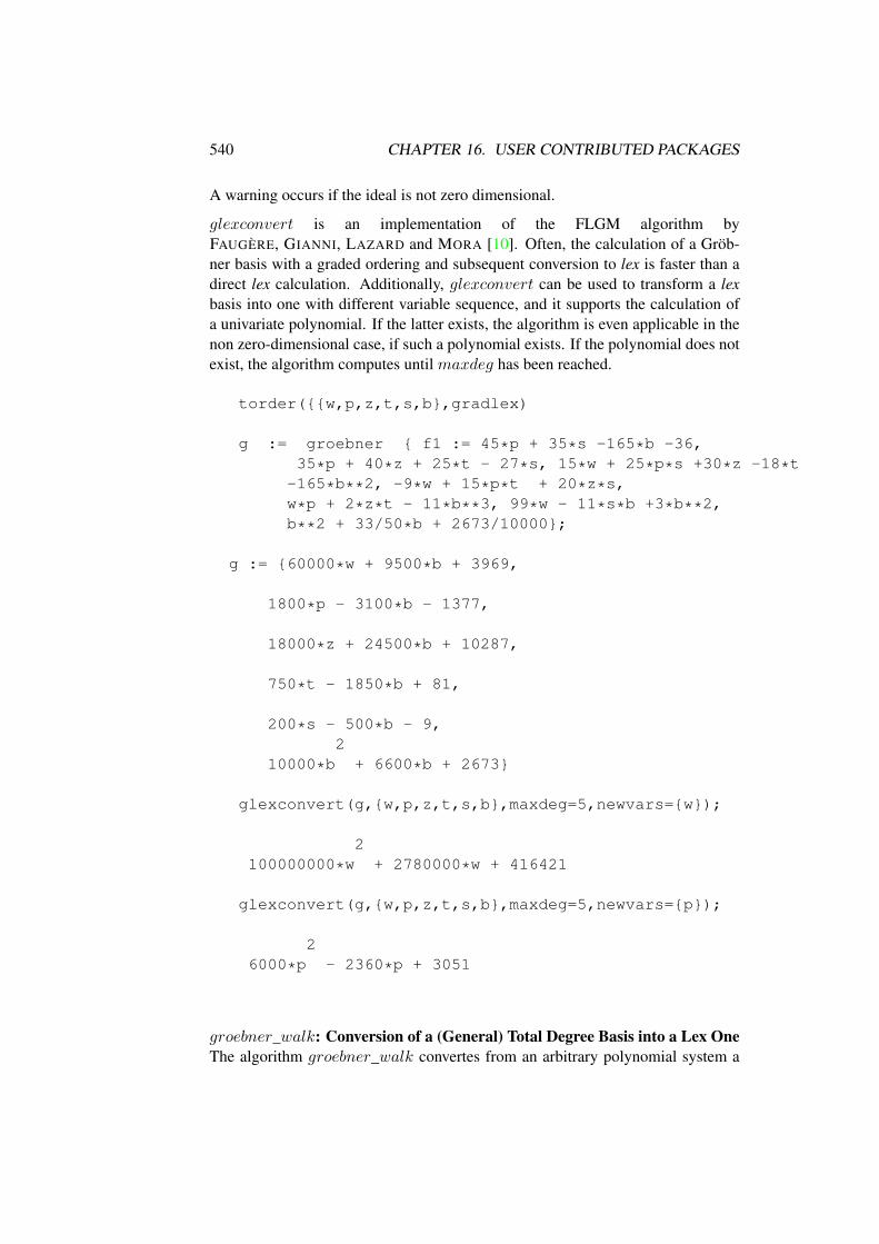
glexconvert is an implementation of the FLGM algorithm byFAUGÈRE, GIANNI, LAZARD and MORA [10]. Often, the calculation of a Gröb-ner basis with a graded ordering and subsequent conversion to lex is faster than adirect lex calculation. Additionally, glexconvert can be used to transform a lexbasis into one with different variable sequence, and it supports the calculation ofa univariate polynomial. If the latter exists, the algorithm is even applicable in thenon zero-dimensional case, if such a polynomial exists. If the polynomial does notexist, the algorithm computes until maxdeg has been reached.

torder({{w,p,z,t,s,b},gradlex)

g := groebner { f1 := 45*p + 35*s -165*b -36,35*p + 40*z + 25*t - 27*s, 15*w + 25*p*s +30*z -18*t-165*b**2, -9*w + 15*p*t + 20*z*s,w*p + 2*z*t - 11*b**3, 99*w - 11*s*b +3*b**2,b**2 + 33/50*b + 2673/10000};

g := {60000*w + 9500*b + 3969,

1800*p - 3100*b - 1377,

18000*z + 24500*b + 10287,

750*t - 1850*b + 81,

200*s - 500*b - 9,2

10000*b + 6600*b + 2673}

glexconvert(g,{w,p,z,t,s,b},maxdeg=5,newvars={w});

2100000000*w + 2780000*w + 416421

glexconvert(g,{w,p,z,t,s,b},maxdeg=5,newvars={p});

26000*p - 2360*p + 3051

groebner_walk: Conversion of a (General) Total Degree Basis into a Lex OneThe algorithm groebner_walk convertes from an arbitrary polynomial system a

541

graduated basis of the given variable sequence to a lex one of the same sequence.The job is done by computing a sequence of Gröbner bases of correspondig mono-mial ideals, lifting the original system each time. The algorithm has been described(more generally) by [2],[3],[1] and [8]. groebner_walk should be only called, ifthe direct calculation of a lex Gröbner base does not work. The computation ofgroebner_walk includes some overhead (e. g. the computation divides poly-nomials). Normally torder must be called before to define the variables and thevariable sorting. The reordering of variables makes no sense with groebner_walk;so do not call groebner_walk with groebopt on!

groebner_walk gwhere g is a polynomial ideal basis computed under gradlex or underweighted with a one–element, non zero weight vector with only one ele-ment, repeated for each variable. The result is a corresponding lex basis (ifthat is computable), independet of the degree of the ideal (even for non zerodegree ideals). The variabe gvarslast is not set.

groebnerf : Factorizing Gröbner Bases

Background If Gröbner bases are computed in order to solve systems of equat-ions or to find the common roots of systems of polynomials, the factorizing versionof the Buchberger algorithm can be used. The theoretical background is simple: ifa polynomial p can be represented as a product of two (or more) polynomials, e.g.h = f ∗g, then h vanishes if and only if one of the factors vanishes. So if during thecalculation of a Gröbner basis h of the above form is detected, the whole problemcan be split into two (or more) disjoint branches. Each of the branches is simplerthan the complete problem; this saves computing time and space. The result ofthis type of computation is a list of (partial) Gröbner bases; the solution set of theoriginal problem is the union of the solutions of the partial problems, ignoring themultiplicity of an individual solution. If a branch results in a basis {1}, then thereis no common zero, i.e. no additional solution for the original problem, contributedby this branch.

groebnerf Call The syntax of groebnerf is the same as for groebner.

groebnerf({exp1, exp2, . . . , expm}[, {}, {nz1, . . . nzk});

where {exp1, exp2, . . . , expm} is a given list of expressions or equations, and{nz1, . . . nzk} is an optional list of polynomials known to be non-zero.

groebnerf tries to separate polynomials into individual factors and to branch thecomputation in a recursive manner (factorization tree). The result is a list of partialGröbner bases. If no factorization can be found or if all branches but one lead to


the trivial basis {1}, the result has only one basis; nevertheless it is a list of listsof polynomials. If no solution is found, the result will be {{1}}. Multiplicities(one factor with a higher power, the same partial basis twice) are deleted as earlyas possible in order to speed up the calculation. The factorizing is controlled bysome switches.

As a side effect, the sequence of variables is stored as a REDUCE list in the sharedvariable

gvarslast .

If gltbasis is on, a corresponding list of leading term bases is also produced and isavailable in the variable gltb.

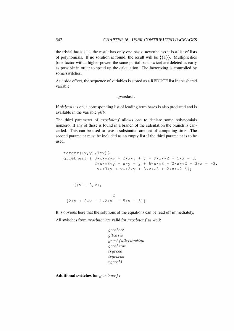
The third parameter of groebnerf allows one to declare some polynomialsnonzero. If any of these is found in a branch of the calculation the branch is can-celled. This can be used to save a substantial amount of computing time. Thesecond parameter must be included as an empty list if the third parameter is to beused.

torder({x,y},lex)$groebnerf { 3*x**2*y + 2*x*y + y + 9*x**2 + 5*x = 3,

2*x**3*y - x*y - y + 6*x**3 - 2*x**2 - 3*x = -3,x**3*y + x**2*y + 3*x**3 + 2*x**2 \};

{{y - 3,x},

2{2*y + 2*x - 1,2*x - 5*x - 5}}

It is obvious here that the solutions of the equations can be read off immediately.

All switches from groebner are valid for groebnerf as well:

groeboptgltbasisgroebfullreductiongroebstattrgroebtrgroebsrgroeb1

Additional switches for groebnerf :

543

trgroebr – All intermediate partial basis are printed when detected.

By default trgroebr is off.

groebmonfac groebresmax groebrestrictionThese variables are described in the following paragraphs.

Suppression of Monomial Factors The factorization in groebnerf is controlledby the following switches and variables. The variable groebmonfac is connectedto the handling of “monomial factors”. A monomial factor is a product of variablepowers occurring as a factor, e.g. x ∗ ∗2 ∗ y in x ∗ ∗3 ∗ y − 2 ∗ x ∗ ∗2 ∗ y ∗ ∗2. Amonomial factor represents a solution of the type “x = 0 or y = 0” with a certainmultiplicity. With groebnerf the multiplicity of monomial factors is lowered tothe value of the shared variable

groebmonfac

which by default is 1 (= monomial factors remain present, but their multiplicity isbrought down). With

groebmonfac := 0

the monomial factors are suppressed completely.

Limitation on the Number of Results The shared variable

groebresmax

controls the number of partial results. Its default value is 300. If groebresmaxpartial results are calculated, the calculation is terminated. groebresmax countsall branches, including those which are terminated (have been computed already),give no contribution to the result (partial basis 1), or which are unified in the resultwith other (partial) bases. So the resulting number may be much smaller. Whenthe limit of groeresmax is reached, a warning

GROEBRESMAX limit reached

is issued; this warning in any case has to be taken as a serious one. For "nor-mal" calculations the groebresmax limit is not reached. groebresmax is a sharedvariable (with an integer value); it can be set in the algebraic mode to a different(positive integer) value.

Restriction of the Solution Space In some applications only a subset of thecomplete solution set of a given set of equations is relevant, e.g. only nonnegative


values or positive definite values for the variables. A significant amount of com-puting time can be saved if nonrelevant computation branches can be terminatedearly.

Positivity: If a polynomial has no (strictly) positive zero, then every system con-taining it has no nonnegative or strictly positive solution. Therefore, the Buch-berger algorithm tests the coefficients of the polynomials for equal sign if re-quested. For example, in 13 ∗ x + 15 ∗ y ∗ z can be zero with real nonnegativevalues for x, y and z only if x = 0 and y = 0 or z = 0; this is a sort of “factoriza-tion by restriction”. A polynomial 13 ∗ x+ 15 ∗ y ∗ z + 20 never can vanish withnonnegative real variable values.

Zero point: If any polynomial in an ideal has an absolute term, the ideal cannothave the origin point as a common solution.

By setting the shared variable

groebrestriction

groebnerf is informed of the type of restriction the user wants to impose on thesolutions:

groebrestiction:=nonnegative;only nonnegative real solutions are of interest

groebrestriction:=positive;only nonnegative and nonzero solutions are of interest

groebrestriction:=zeropoint;only solution sets which contain the point {0, 0, . . . , 0} are or interest.

If groebnerf detects a polynomial which formally conflicts with the restriction, iteither splits the calculation into separate branches, or, if a violation of the restric-tion is determined, it cancels the actual calculation branch.

greduce, preduce: Reduction of Polynomials

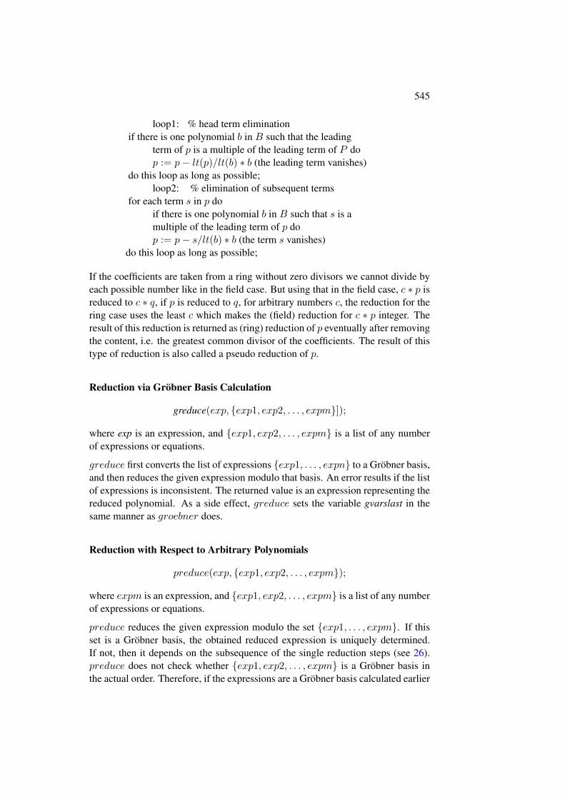
Background Reduction of a polynomial “p” modulo a given sets of polynomials“b” is done by the reduction algorithm incorporated in the Buchberger algorithm.Informally it can be described for polynomials over a field as follows:

545

loop1: % head term eliminationif there is one polynomial b in B such that the leading

term of p is a multiple of the leading term of P dop := p− lt(p)/lt(b) ∗ b (the leading term vanishes)

do this loop as long as possible;loop2: % elimination of subsequent terms

for each term s in p doif there is one polynomial b in B such that s is amultiple of the leading term of p dop := p− s/lt(b) ∗ b (the term s vanishes)

do this loop as long as possible;

If the coefficients are taken from a ring without zero divisors we cannot divide byeach possible number like in the field case. But using that in the field case, c ∗ p isreduced to c ∗ q, if p is reduced to q, for arbitrary numbers c, the reduction for thering case uses the least c which makes the (field) reduction for c ∗ p integer. Theresult of this reduction is returned as (ring) reduction of p eventually after removingthe content, i.e. the greatest common divisor of the coefficients. The result of thistype of reduction is also called a pseudo reduction of p.

Reduction via Gröbner Basis Calculation

greduce(exp, {exp1, exp2, . . . , expm}]);

where exp is an expression, and {exp1, exp2, . . . , expm} is a list of any numberof expressions or equations.

greduce first converts the list of expressions {exp1, . . . , expn} to a Gröbner basis,and then reduces the given expression modulo that basis. An error results if the listof expressions is inconsistent. The returned value is an expression representing thereduced polynomial. As a side effect, greduce sets the variable gvarslast in thesame manner as groebner does.

Reduction with Respect to Arbitrary Polynomials

preduce(exp, {exp1, exp2, . . . , expm});

where expm is an expression, and {exp1, exp2, . . . , expm} is a list of any numberof expressions or equations.

preduce reduces the given expression modulo the set {exp1, . . . , expm}. If thisset is a Gröbner basis, the obtained reduced expression is uniquely determined.If not, then it depends on the subsequence of the single reduction steps (see 26).preduce does not check whether {exp1, exp2, . . . , expm} is a Gröbner basis inthe actual order. Therefore, if the expressions are a Gröbner basis calculated earlier


with a variable sequence given explicitly or modified by optimization, the propervariable sequence and term order must be activated first.

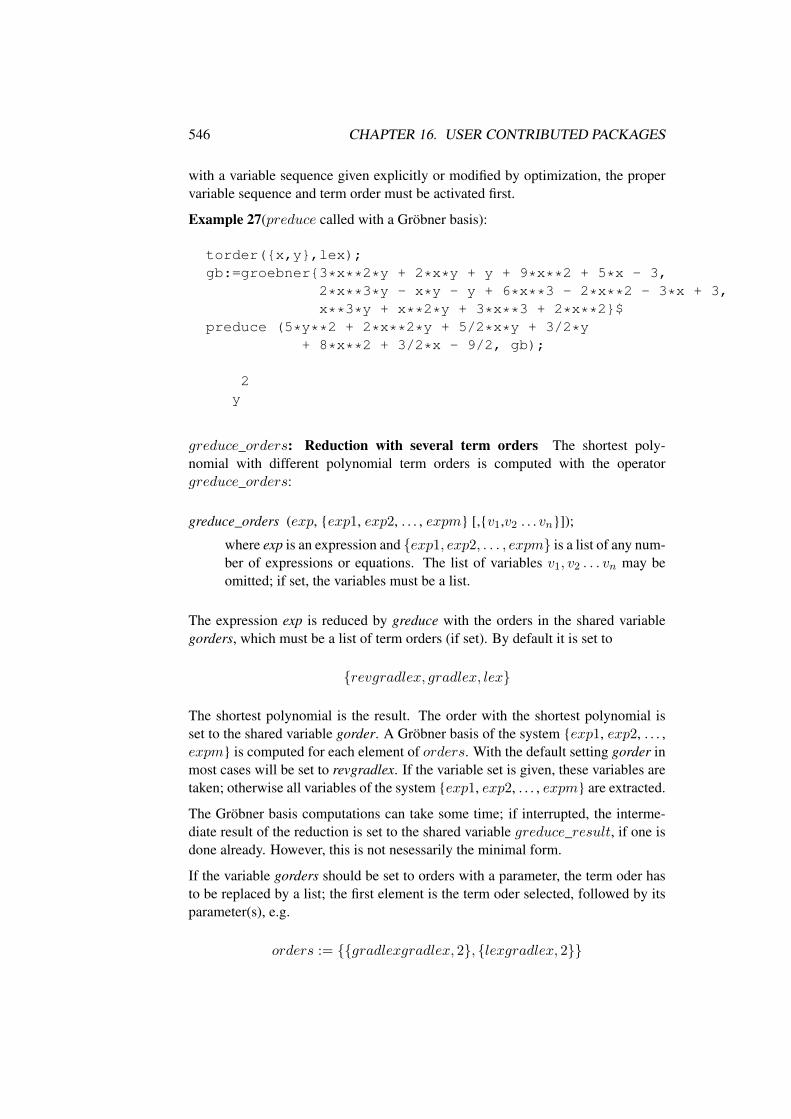
Example 27(preduce called with a Gröbner basis):

torder({x,y},lex);gb:=groebner{3*x**2*y + 2*x*y + y + 9*x**2 + 5*x - 3,

2*x**3*y - x*y - y + 6*x**3 - 2*x**2 - 3*x + 3,x**3*y + x**2*y + 3*x**3 + 2*x**2}$

preduce (5*y**2 + 2*x**2*y + 5/2*x*y + 3/2*y+ 8*x**2 + 3/2*x - 9/2, gb);

2y

greduce_orders: Reduction with several term orders The shortest poly-nomial with different polynomial term orders is computed with the operatorgreduce_orders:

greduce_orders (exp, {exp1, exp2, . . . , expm} [,{v1,v2 . . . vn}]);

where exp is an expression and {exp1, exp2, . . . , expm} is a list of any num-ber of expressions or equations. The list of variables v1, v2 . . . vn may beomitted; if set, the variables must be a list.

The expression exp is reduced by greduce with the orders in the shared variablegorders, which must be a list of term orders (if set). By default it is set to

{revgradlex, gradlex, lex}

The shortest polynomial is the result. The order with the shortest polynomial isset to the shared variable gorder. A Gröbner basis of the system {exp1, exp2, . . . ,expm} is computed for each element of orders. With the default setting gorder inmost cases will be set to revgradlex. If the variable set is given, these variables aretaken; otherwise all variables of the system {exp1, exp2, . . . , expm} are extracted.

The Gröbner basis computations can take some time; if interrupted, the interme-diate result of the reduction is set to the shared variable greduce_result, if one isdone already. However, this is not nesessarily the minimal form.

If the variable gorders should be set to orders with a parameter, the term oder hasto be replaced by a list; the first element is the term oder selected, followed by itsparameter(s), e.g.

orders := {{gradlexgradlex, 2}, {lexgradlex, 2}}

547

Reduction Tree In some case not only are the results produced by greduce andpreduce of interest, but the reduction process is of some value too. If the switch

groebprot

is set on, groebner, greduce and preduce produce as a side effect a trace of theirwork as a REDUCE list of equations in the shared variable

groebprotfile.

Its value is a list of equations with a variable “candidate” playing the role of theobject to be reduced. The polynomials are cited as “poly1”, “poly2”, . . . . If read asassignments, these equations form a program which leads from the reduction inputto its result. Note that, due to the pseudo reduction with a ring as the coefficientdomain, the input coefficients may be changed by global factors.


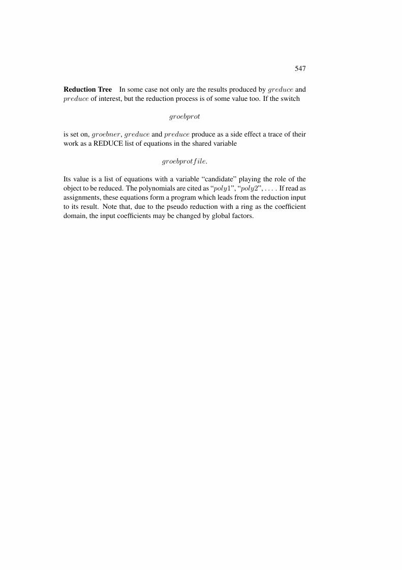
Example 28

on groebprot $preduce (5 ∗ y ∗ ∗2 + 2 ∗ x ∗ ∗2 ∗ y + 5/2 ∗ x ∗ y + 3/2 ∗ y + 8 ∗ x ∗ ∗2

+3/2 ∗ x− 9/2, gb);

2y

groebprotfile;

2 2 2{candidate=4*x *y + 16*x + 5*x*y + 3*x + 10*y + 3*y - 9,

2poly1=8*x - 2*y + 5*y + 3,

3 2poly2=2*y - 3*y - 16*y + 21,candidate=2*candidate,candidate= - x*y*poly1 + candidate,candidate= - 4*x*poly1 + candidate,candidate=4*candidate,

3candidate= - y *poly1 + candidate,candidate=2*candidate,

2candidate= - 3*y *poly1 + candidate,candidate=13*y*poly1 + candidate,candidate=candidate + 6*poly1,

2candidate= - 2*y *poly2 + candidate,candidate= - y*poly2 + candidate,candidate=candidate + 6*poly2}

549

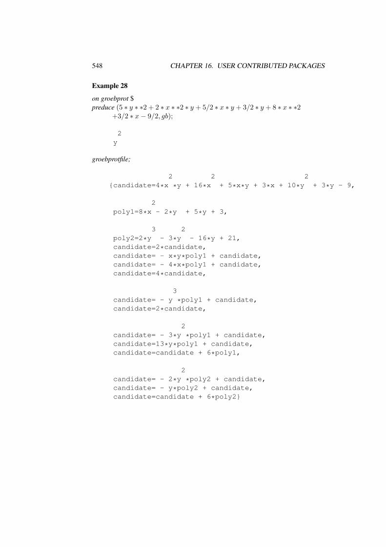
This means

16(5y2 + 2x2y +5

2xy +

3

2y + 8x2 +

3

2x− 9

2) =

(−8xy − 32x− 2y3 − 3y2 + 13y + 6)poly1

+(−2y2 − 2y + 6)poly2 + y2.

Tracing with groebnert and preducet

Given a set of polynomials {f1, . . . , fk} and their Gröbner basis {g1, . . . , gl}, it iswell known that there are matrices of polynomials Cij and Dji such that

fi =∑j

Cijgj and gj =∑i

Djifi

and these relations are needed explicitly sometimes. In BUCHBERGER [6], suchcases are described in the context of linear polynomial equations. The standardtechnique for computing the above formulae is to perform Gröbner reductions,keeping track of the computation in terms of the input data. In the current packagesuch calculations are performed with (an internally hidden) cofactor technique:the user has to assign unique names to the input expressions and the arithmeticcombinations are done with the expressions and with their names simultaneously.So the result is accompanied by an expression which relates it algebraically to theinput values.

There are two complementary operators with this feature: groebnert and preducet;functionally they correspond to groebner and preduce. However, the sets of ex-pressions here must be equations with unique single identifiers on their left sideand the lhs are interpreted as names of the expressions. Their results are sets ofequations (groebnert) or equations (preducet), where a lhs is the computed value,while the rhs is its equivalent in terms of the input names.

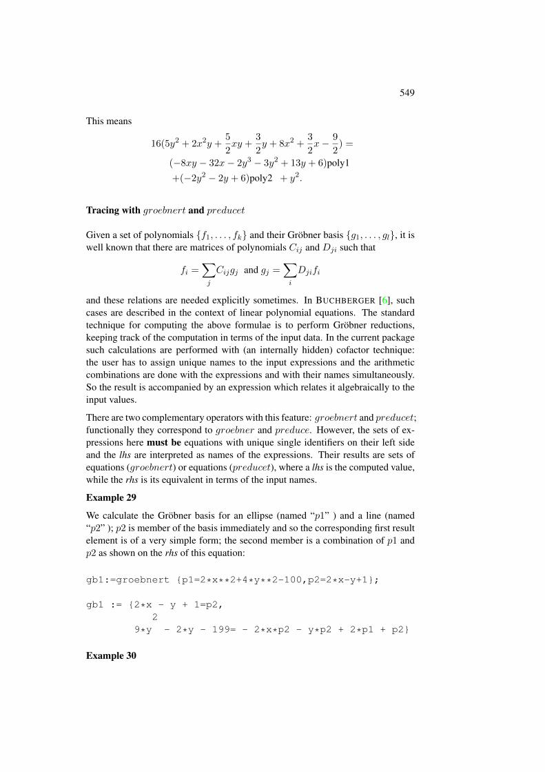
Example 29

We calculate the Gröbner basis for an ellipse (named “p1” ) and a line (named“p2” ); p2 is member of the basis immediately and so the corresponding first resultelement is of a very simple form; the second member is a combination of p1 andp2 as shown on the rhs of this equation:

gb1:=groebnert {p1=2*x**2+4*y**2-100,p2=2*x-y+1};

gb1 := {2*x - y + 1=p2,2

9*y - 2*y - 199= - 2*x*p2 - y*p2 + 2*p1 + p2}

Example 30


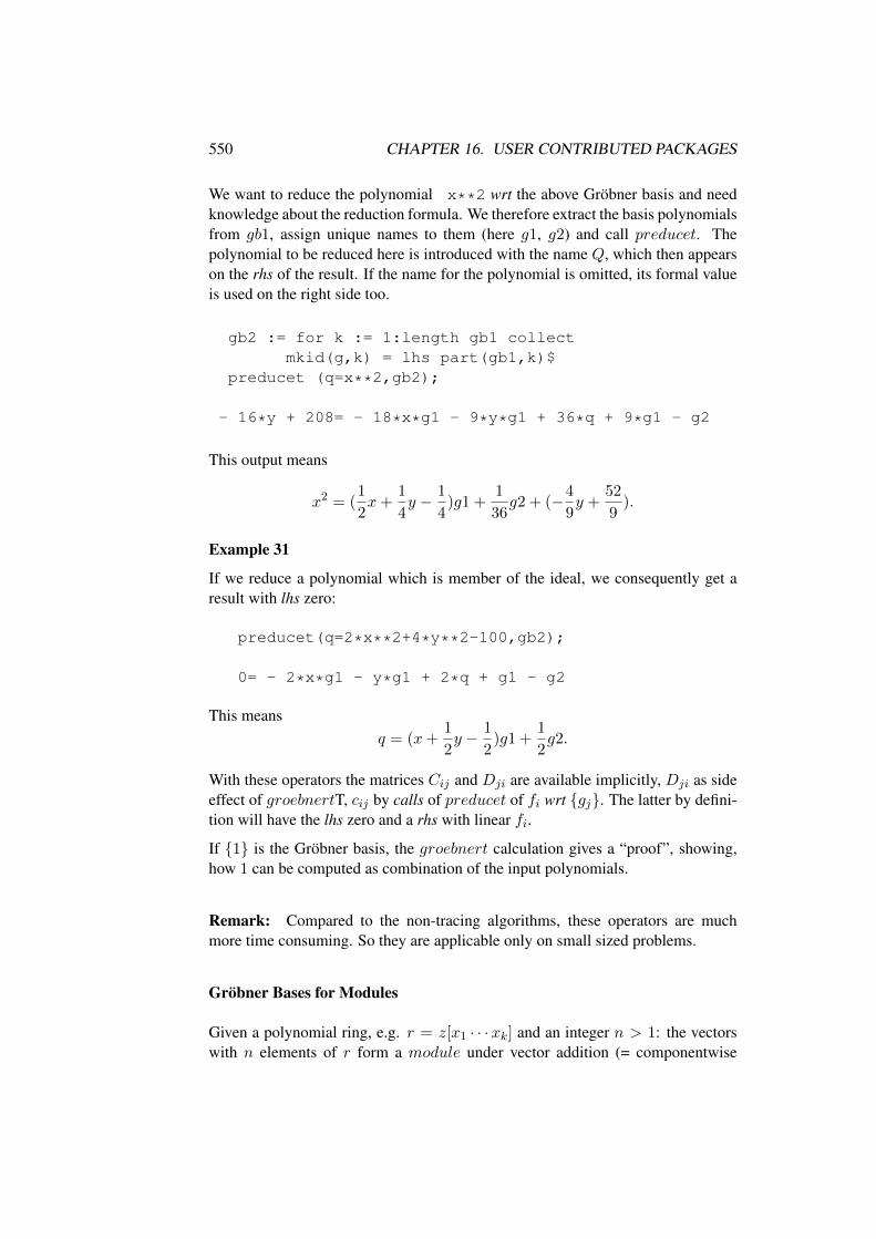
We want to reduce the polynomial x**2 wrt the above Gröbner basis and needknowledge about the reduction formula. We therefore extract the basis polynomialsfrom gb1, assign unique names to them (here g1, g2) and call preducet. Thepolynomial to be reduced here is introduced with the name Q, which then appearson the rhs of the result. If the name for the polynomial is omitted, its formal valueis used on the right side too.

gb2 := for k := 1:length gb1 collectmkid(g,k) = lhs part(gb1,k)$

preducet (q=x**2,gb2);

- 16*y + 208= - 18*x*g1 - 9*y*g1 + 36*q + 9*g1 - g2

This output means

x2 = (1

2x+

1

4y − 1

4)g1 +

1

36g2 + (−4

9y +

52

9).

Example 31

If we reduce a polynomial which is member of the ideal, we consequently get aresult with lhs zero:

preducet(q=2*x**2+4*y**2-100,gb2);

0= - 2*x*g1 - y*g1 + 2*q + g1 - g2

This meansq = (x+

1

2y − 1

2)g1 +

1

2g2.

With these operators the matrices Cij and Dji are available implicitly, Dji as sideeffect of groebnertT, cij by calls of preducet of fi wrt {gj}. The latter by defini-tion will have the lhs zero and a rhs with linear fi.

If {1} is the Gröbner basis, the groebnert calculation gives a “proof”, showing,how 1 can be computed as combination of the input polynomials.

Remark: Compared to the non-tracing algorithms, these operators are muchmore time consuming. So they are applicable only on small sized problems.

Gröbner Bases for Modules

Given a polynomial ring, e.g. r = z[x1 · · ·xk] and an integer n > 1: the vectorswith n elements of r form a module under vector addition (= componentwise

551

addition) and multiplication with elements of r. For a submodule given by a finitebasis a Gröbner basis can be computed, and the facilities of the groebner packagecan be used except the operators groebnerf and groesolve.

The vectors are encoded using auxiliary variables which represent the unit vectorsin the module. E.g. using v1, v2, v3 the module element [x2

1, 0, x1 − x2] is repre-sented as x2

1v1 + x1v3 − x2v3. The use of v1, v2, v3 as unit vectors is set up byassigning the set of auxiliary variables to the share variable gmodule, e.g.

gmodule := {v1,v2,v3};

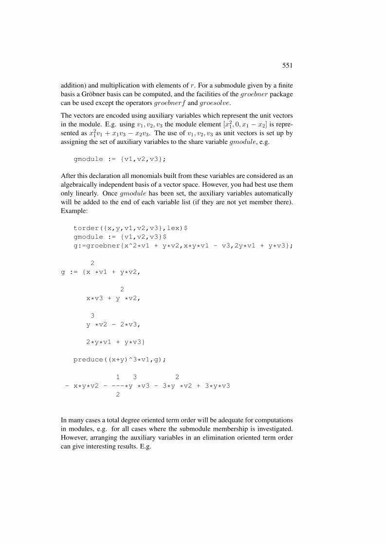
After this declaration all monomials built from these variables are considered as analgebraically independent basis of a vector space. However, you had best use themonly linearly. Once gmodule has been set, the auxiliary variables automaticallywill be added to the end of each variable list (if they are not yet member there).Example:

torder({x,y,v1,v2,v3},lex)$gmodule := {v1,v2,v3}$g:=groebner{x^2*v1 + y*v2,x*y*v1 - v3,2y*v1 + y*v3};

2g := {x *v1 + y*v2,

2x*v3 + y *v2,

3y *v2 - 2*v3,

2*y*v1 + y*v3}

preduce((x+y)^3*v1,g);

1 3 2- x*y*v2 - ---*y *v3 - 3*y *v2 + 3*y*v3

2

In many cases a total degree oriented term order will be adequate for computationsin modules, e.g. for all cases where the submodule membership is investigated.However, arranging the auxiliary variables in an elimination oriented term ordercan give interesting results. E.g.


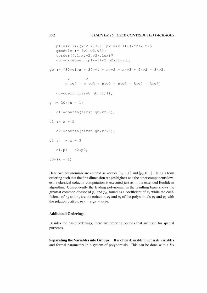
p1:=(x-1)*(x^2-x+3)$ p2:=(x-1)*(x^2+x-5)$gmodule := {v1,v2,v3};torder({v1,x,v2,v3},lex)$gb:=groebner {p1*v1+v2,p2*v1+v3};

gb := {30*v1*x - 30*v1 + x*v2 - x*v3 + 5*v2 - 3*v3,

2 2x *v2 - x *v3 + x*v2 + x*v3 - 5*v2 - 3*v3}

g:=coeffn(first gb,v1,1);

g := 30*(x - 1)

c1:=coeffn(first gb,v2,1);

c1 := x + 5

c2:=coeffn(first gb,v3,1);

c2 := - x - 3

c1*p1 + c2*p2;

30*(x - 1)

Here two polynomials are entered as vectors [p1, 1, 0] and [p2, 0, 1]. Using a termordering such that the first dimension ranges highest and the other components low-est, a classical cofactor computation is executed just as in the extended Euclideanalgorithm. Consequently the leading polynomial in the resulting basis shows thegreatest common divisor of p1 and p2, found as a coefficient of v1 while the coef-ficients of v2 and v3 are the cofactors c1 and c2 of the polynomials p1 and p2 withthe relation gcd(p1, p2) = c1p1 + c2p2.

Additional Orderings

Besides the basic orderings, there are ordering options that are used for specialpurposes.

Separating the Variables into Groups It is often desirable to separate variablesand formal parameters in a system of polynomials. This can be done with a lex

553

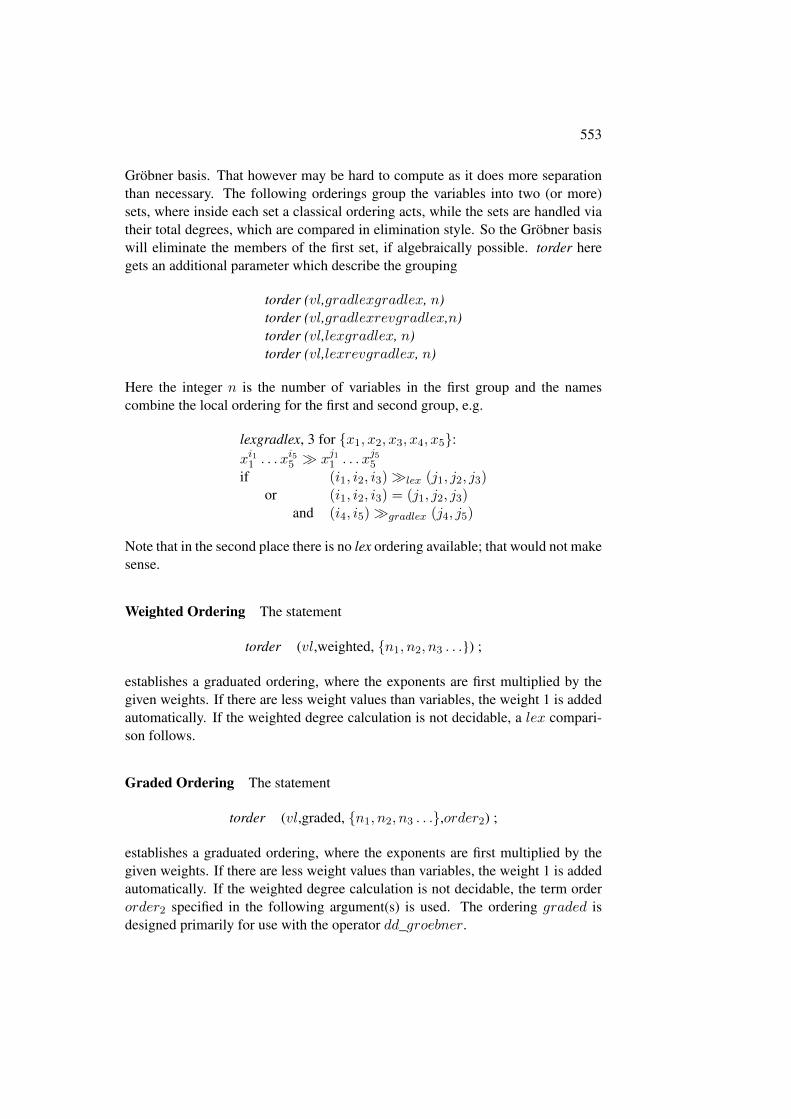
Gröbner basis. That however may be hard to compute as it does more separationthan necessary. The following orderings group the variables into two (or more)sets, where inside each set a classical ordering acts, while the sets are handled viatheir total degrees, which are compared in elimination style. So the Gröbner basiswill eliminate the members of the first set, if algebraically possible. torder heregets an additional parameter which describe the grouping

torder (vl,gradlexgradlex, n)torder (vl,gradlexrevgradlex,n)torder (vl,lexgradlex, n)torder (vl,lexrevgradlex, n)

Here the integer n is the number of variables in the first group and the namescombine the local ordering for the first and second group, e.g.

lexgradlex, 3 for {x1, x2, x3, x4, x5}:xi11 . . . x

i55 � xj11 . . . xj55

if (i1, i2, i3)�lex (j1, j2, j3)or (i1, i2, i3) = (j1, j2, j3)

and (i4, i5)�gradlex (j4, j5)

Note that in the second place there is no lex ordering available; that would not makesense.

Weighted Ordering The statement

torder (vl,weighted, {n1, n2, n3 . . .}) ;

establishes a graduated ordering, where the exponents are first multiplied by thegiven weights. If there are less weight values than variables, the weight 1 is addedautomatically. If the weighted degree calculation is not decidable, a lex compari-son follows.

Graded Ordering The statement

torder (vl,graded, {n1, n2, n3 . . .},order2) ;

establishes a graduated ordering, where the exponents are first multiplied by thegiven weights. If there are less weight values than variables, the weight 1 is addedautomatically. If the weighted degree calculation is not decidable, the term orderorder2 specified in the following argument(s) is used. The ordering graded isdesigned primarily for use with the operator dd_groebner.


Matrix Ordering The statement

torder (vl,matrix, m) ;

wherem is a matrix with integer elements and row length which corresponds to thevariable number. The exponents of each monomial form a vector; two monomialsare compared by multiplying their exponent vectors first with m and comparingthe resulting vector lexicographically. E.g. the unit matrix establishes the classicallex term order mode, a matrix with a first row of ones followed by the rows of aunit matrix corresponds to the gradlex ordering.

The matrix m must have at least as many rows as columns; a non–square matrixcontains redundant rows. The matrix must have full rank, and the top non–zeroelement of each column must be positive.

The generality of the matrix based term order has its price: the computing timespent in the term sorting is significantly higher than with the specialized term or-ders. To overcome this problem, you can compile a matrix term order ; the com-pilation reduces the computing time overhead significantly. If you set the switchcomp on, any new order matrix is compiled when any operator of the groebnerpackage accesses it for the first time. Alternatively you can compile a matrix ex-plicitly

torder_compile(<n>,<m>);

where < n > is a name (an identifier) and < m > is a term order matrix.torder_compile transforms the matrix into a LISP program, which is compiledby the LISP compiler when comp is on or when you generate a fast loadable mod-ule. Later you can activate the new term order by using the name < n > in atorder statement as term ordering mode.

Gröbner Bases for Graded Homogeneous Systems

For a homogeneous system of polynomials under a term order graded, gradlex,revgradlex or weighted a Gröbner Base can be computed with limiting the grade ofthe intermediate s–polynomials:

dd_groebner (d1,d2,{p1, p2, . . .});

where d1 is a non–negative integer and d2 is an integer > d1 or “infinity". A pairof polynomials is considered only if the grade of the lcm of their head terms isbetween d1 and d2. See [4] for the mathematical background. For the term ordersgraded or weighted the (first) weight vector is used for the grade computation.Otherwise the total degree of a term is used.

555

16.28.4 Ideal Decomposition & Equation System Solving

Based on the elementary Gröbner operations, the groebner package offers ad-ditional operators, which allow the decomposition of an ideal or of a system ofequations down to the individual solutions.

Solutions Based on Lex Type Gröbner Bases

groesolve: Solution of a Set of Polynomial Equations The groesolve operatorincorporates a macro algorithm; lexical Gröbner bases are computed by groebnerfand decomposed into simpler ones by ideal decomposition techniques; if alge-braically possible, the problem is reduced to univariate polynomials which aresolved by solve; if rounded is on, numerical approximations are computed forthe roots of the univariate polynomials.

groesolve({exp1, exp2, . . . , expm}[, {var1, var2, . . . , varn}]);

where {exp1, exp2, . . . , expm} is a list of any number of expressions or equations,{var1, var2, . . . , varn} is an optional list of variables.

The result is a set of subsets. The subsets contain the solutions of the polynomialequations. If there are only finitely many solutions, then each subset is a set ofexpressions of triangular type {exp1, exp2, . . . , expn}, where exp1 depends onlyon var1, exp2 depends only on var1 and var2 etc. until expn which dependson var1, . . . , varn. This allows a successive determination of the solution com-ponents. If there are infinitely many solutions, some subsets consist in less thann expressions. By considering some of the variables as “free parameters”, thesesubsets are usually again of triangular type.

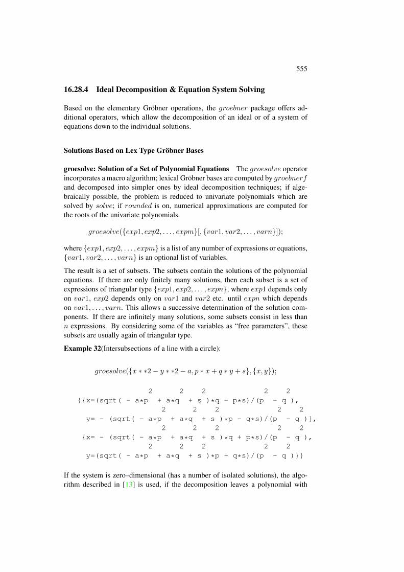
Example 32(Intersubsections of a line with a circle):

groesolve({x ∗ ∗2− y ∗ ∗2− a, p ∗ x+ q ∗ y + s}, {x, y});

2 2 2 2 2{{x=(sqrt( - a*p + a*q + s )*q - p*s)/(p - q ),

2 2 2 2 2y= - (sqrt( - a*p + a*q + s )*p - q*s)/(p - q )},

2 2 2 2 2{x= - (sqrt( - a*p + a*q + s )*q + p*s)/(p - q ),

2 2 2 2 2y=(sqrt( - a*p + a*q + s )*p + q*s)/(p - q )}}

If the system is zero–dimensional (has a number of isolated solutions), the algo-rithm described in [13] is used, if the decomposition leaves a polynomial with


mixed leading term. Hillebrand has written the article and Möller was the tutor ofthis job.

The reordering of the groesolve variables is controlled by the REDUCE switchvaropt. If varopt is on (which is the default of varopt), the variable sequenceis optimized (the variables are reordered). If varopt is off , the given variablesequence is taken (if no variables are given, the order of the REDUCE systemis taken instead). In general, the reordering of the variables makes the Gröbnerbasis computation significantly faster. A variable dependency, declare by one (orseveral) depend statements, is regarded (if varopt is on). The switch groebopt hasno meaning for groesolve; it is stored during its processing.

groepostproc: Postprocessing of a Gröbner Basis In many cases, it is difficultto do the general Gröbner processing. If a Gröbner basis with a lex ordering iscalculated already (e.g., by very individual parameter settings), the solutions canbe derived from it by a call to groepostproc. groesolve is functionally equivalentto a call to groebnerf and subsequent calls to groepostproc for each partial basis.

groepostproc({exp1, exp2, . . . , expm}[, {var1, var2, . . . , varn}]);

where {exp1, exp2, . . . , expm} is a list of any number of expressions,{var1, var2, . . . , varn} is an optional list of variables. The expressions mustbe a lex Gröbner basis with the given variables; the ordering must be still active.

The result is the same as with groesolve.

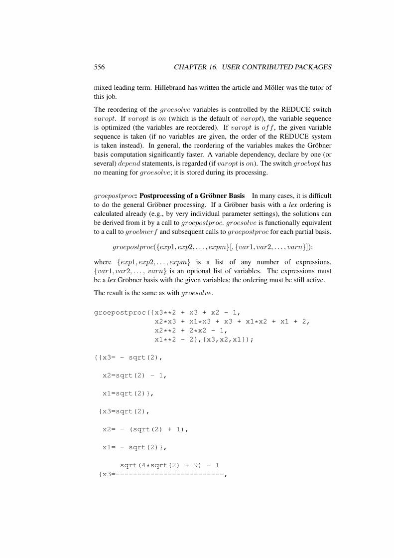
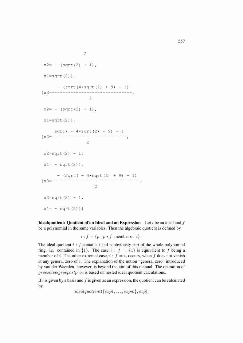
groepostproc({x3**2 + x3 + x2 - 1,x2*x3 + x1*x3 + x3 + x1*x2 + x1 + 2,x2**2 + 2*x2 - 1,x1**2 - 2},{x3,x2,x1});

{{x3= - sqrt(2),

x2=sqrt(2) - 1,

x1=sqrt(2)},

{x3=sqrt(2),

x2= - (sqrt(2) + 1),

x1= - sqrt(2)},

sqrt(4*sqrt(2) + 9) - 1{x3=-------------------------,

557

2

x2= - (sqrt(2) + 1),

x1=sqrt(2)},

- (sqrt(4*sqrt(2) + 9) + 1){x3=------------------------------,

2

x2= - (sqrt(2) + 1),

x1=sqrt(2)},

sqrt( - 4*sqrt(2) + 9) - 1{x3=----------------------------,

2

x2=sqrt(2) - 1,

x1= - sqrt(2)},

- (sqrt( - 4*sqrt(2) + 9) + 1){x3=---------------------------------,

2

x2=sqrt(2) - 1,

x1= - sqrt(2)}}

Idealquotient: Quotient of an Ideal and an Expression Let i be an ideal and fbe a polynomial in the same variables. Then the algebraic quotient is defined by

i : f = {p | p ∗ f member of i} .

The ideal quotient i : f contains i and is obviously part of the whole polynomialring, i.e. contained in {1}. The case i : f = {1} is equivalent to f being amember of i. The other extremal case, i : f = i, occurs, when f does not vanishat any general zero of i. The explanation of the notion “general zero” introducedby van der Waerden, however, is beyond the aim of this manual. The operation ofgroesolve/groepostproc is based on nested ideal quotient calculations.

If i is given by a basis and f is given as an expression, the quotient can be calculatedby

idealquotient({exp1, . . . , expm}, exp);


where {exp1, exp2, . . . , expm} is a list of any number of expressions or equations,exp is a single expression or equation.

idealquotient calculates the algebraic quotient of the ideal i with the basis{exp1, exp2, . . . , expm} and exp with respect to the variables given or extracted.{exp1, exp2, . . . , expm} is not necessarily a Gröbner basis. The result is the Gröb-ner basis of the quotient.

Saturation: Saturation of an Ideal and an Expression The saturation op-erator computes the quotient on an ideal and an arbitrary power of an expressionexp ∗ ∗n with arbitrary n. The call is

saturation({exp1, . . . , expm}, exp);

where {exp1, exp2, . . . , expm} is a list of any number of expressions or equations,exp is a single expression or equation.

saturation calls idealquotient several times, until the result is stable, and returnsit.

Operators for Gröbner Bases in all Term Orderings

In some cases where no Gröbner basis with lexical ordering can be calculated, acalculation with a total degree ordering is still possible. Then the Hilbert polyno-mial gives information about the dimension of the solutions space and for finite setsof solutions univariate polynomials can be calculated. The solutions of the equat-ion system then is contained in the cross product of all solutions of all univariatepolynomials.

Hilbertpolynomial: Hilbert Polynomial of an Ideal This algorithm was con-tributed by JOACHIM HOLLMAN, Royal Institute of Technology, Stockholm (pri-vate communication).

hilbertpolynomial({exp1, . . . , expm}) ;

where {exp1, . . . , expm} is a list of any number of expressions or equations.

hilertpolynomial calculates the Hilbert polynomial of the ideal with basis{exp1, . . . , expm} with respect to the variables given or extracted providedthe given term ordering is compatible with the degree, such as the gradlex-or revgradlex-ordering. The term ordering of the basis must be active and{exp1, . . ., expm} should be a Gröbner basis with respect to this ordering. TheHilbert polynomial gives information about the cardinality of solutions of the sys-tem {exp1, . . . , expm}: if the Hilbert polynomial is an integer, the system has

559

only a discrete set of solutions and the polynomial is identical with the numberof solutions counted with their multiplicities. Otherwise the degree of the Hilbertpolynomial is the dimension of the solution space.

If the Hilbert polynomial is not a constant, it is constructed with the variable “x”regardless of whether x is member of {var1, . . . , varn} or not. The value of thispolynomial at sufficiently large numbers “x” is the difference of the dimension ofthe linear vector space of all polynomials of degree ≤ x minus the dimension ofthe subspace of all polynomials of degree ≤ x which belong also to the ideal.

x must be an undefined variable or the value of x must be an undefined variable;otherwise a warning is given and a new (generated) variable is taken instead.

Remark: The number of zeros in an ideal and the Hilbert polynomial dependonly on the leading terms of the Gröbner basis. So if a subsequent Hilbert calcu-lation is planned, the Gröbner calculation should be performed with on gltbasisand the value of gltb (or its elements in a groebnerf context) should be given tohilbertpolynomial. In this manner, a lot of computing time can be saved in thecase of long calculations.

16.28.5 Calculations “by Hand”

The following operators support explicit calculations with polynomials in a dis-tributive representation at the REDUCE top level. So they allow one to do Gröbnertype evaluations stepwise by separate calls. Note that the normal REDUCE arith-metic can be used for arithmetic combinations of monomials and polynomials.

Representing Polynomials in Distributive Form

gsortp;

where p is a polynomial or a list of polynomials.

If p is a single polynomial, the result is a reordered version of p in the distributiverepresentation according to the variables and the current term order mode; if pis a list, its members are converted into distributive representation and the resultis the list sorted by the term ordering of the leading terms; zero polynomials areeliminated from the result.

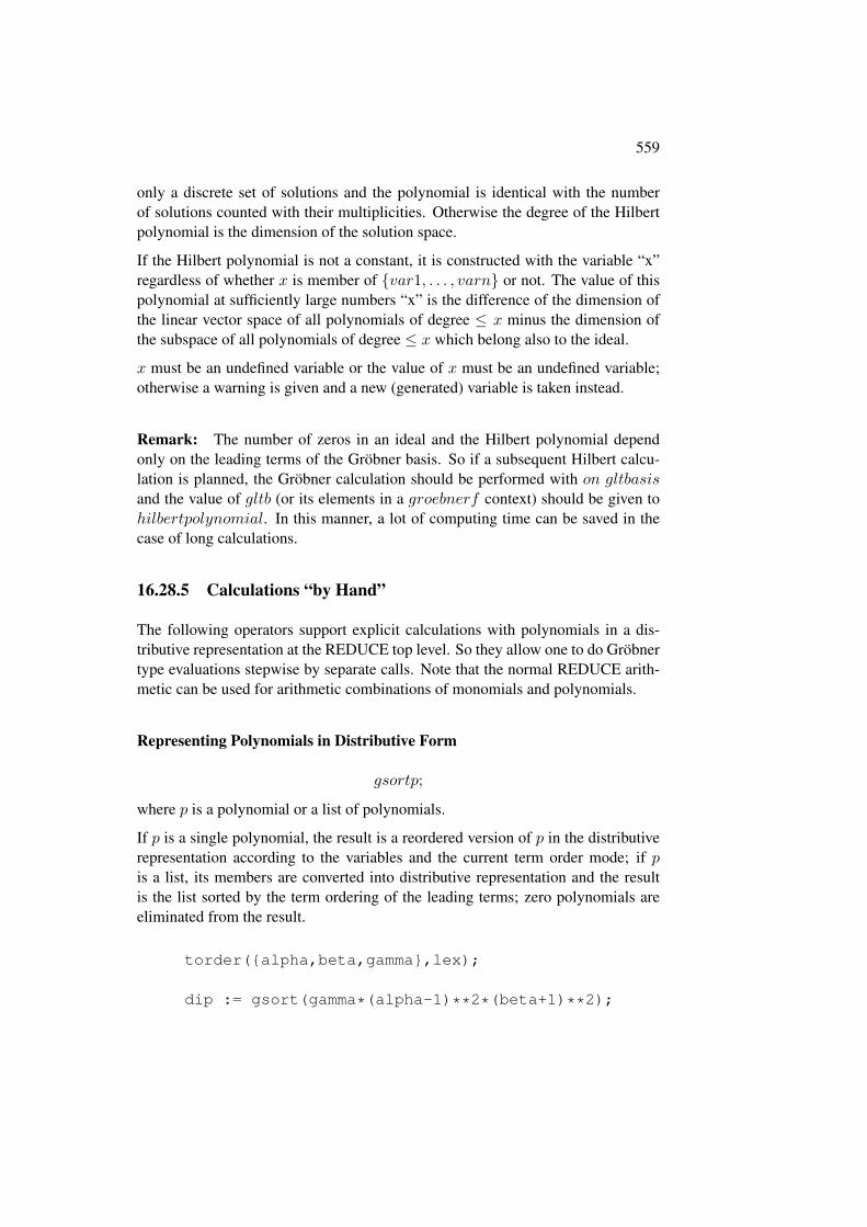
torder({alpha,beta,gamma},lex);

dip := gsort(gamma*(alpha-1)**2*(beta+1)**2);


2 2 2dip := alpha *beta *gamma + 2*alpha *beta*gamma

2 2+ alpha *gamma - 2*alpha*beta *gamma - 4*alpha*beta*gamma

2- 2*alpha*gamma + beta *gamma + 2*beta*gamma + gamma

Splitting of a Polynomial into Leading Term and Reductum

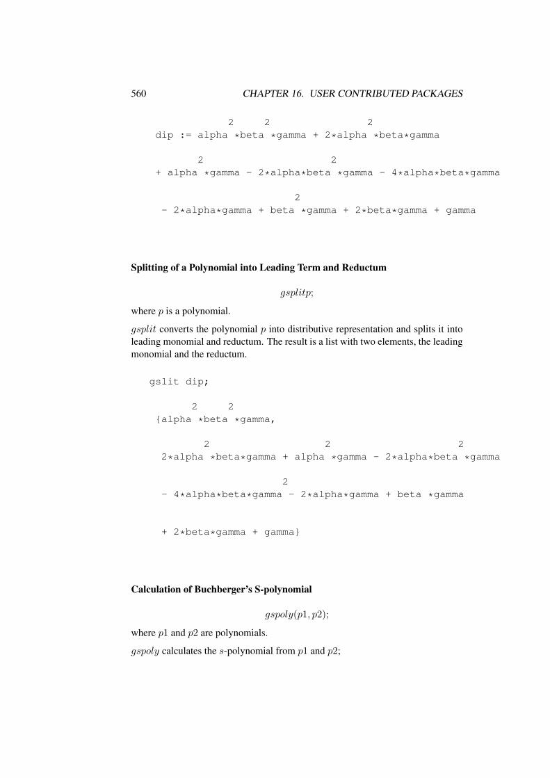
gsplitp;

where p is a polynomial.

gsplit converts the polynomial p into distributive representation and splits it intoleading monomial and reductum. The result is a list with two elements, the leadingmonomial and the reductum.

gslit dip;

2 2{alpha *beta *gamma,

2 2 22*alpha *beta*gamma + alpha *gamma - 2*alpha*beta *gamma

2- 4*alpha*beta*gamma - 2*alpha*gamma + beta *gamma

+ 2*beta*gamma + gamma}

Calculation of Buchberger’s S-polynomial

gspoly(p1, p2);

where p1 and p2 are polynomials.

gspoly calculates the s-polynomial from p1 and p2;

561

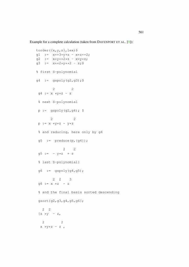
Example for a complete calculation (taken from DAVENPORT ET AL. [9]):

torder({x,y,z},lex)$g1 := x**3*y*z - x*z**2;g2 := x*y**2*z - x*y*z;g3 := x**2*y**2 - z;$

% first S-polynomial

g4 := gspoly(g2,g3);$

2 2g4 := x *y*z - z

% next S-polynomial

p := gspoly(g2,g4); $

2 2p := x *y*z - y*z

% and reducing, here only by g4

g5 := preduce(p,{g4});

2 2g5 := - y*z + z

% last S-polynomial}

g6 := gspoly(g4,g5);

2 2 3g6 := x *z - z

% and the final basis sorted descending

gsort{g2,g3,g4,g5,g6};

2 2{x *y - z,

2 2x *y*z - z ,


2 2 3x *z - z ,

2x*y *z - x*y*z,

2 2- y*z + z }

Bibliography

[1] Beatrice Amrhein and Oliver Gloor. The fractal walk. In Bruno Buchbergeran Franz Winkler, editor, Gröbner Bases and Applications, volume 251 ofLMS, pages 305 –322. Cambridge University Press, February 1998.

[2] Beatrice Amrhein, Oliver Gloor, and Wolfgang Kuechlin. How fast doesthe walk run? In Alain Carriere and Louis Remy Oudin, editors, 5th RhineWorkshop on Computer Algebra, volume PR 801/96, pages 8.1 – 8.9. InstitutFranco–Allemand de Recherches de Saint–Louis, January 1996.

[3] Beatrice Amrhein, Oliver Gloor, and Wolfgang Kuechlin. Walking faster. InJ. Calmet and C. Limongelli, editors, Design and Implementation of SymbolicComputation Systems, volume 1128 of Lecture Notes in Computer Science,pages 150 –161. Springer, 1996.

[4] Thomas Becker and Volker Weispfenning. Gröbner Bases. Springer, 1993.

[5] W. Boege, R. Gebauer, and H. Kredel. Some examples for solving systems ofalgebraic equations by calculating Gröbner bases. J. Symbolic Computation,2(1):83–98, March 1986.

[6] Bruno Buchberger. Gröbner bases: An algorithmic method in polynomialideal theory. In N. K. Bose, editor, Progress, directions and open problems inmultidimensional systems theory, pages 184–232. Dordrecht: Reidel, 1985.

[7] Bruno Buchberger. Applications of Gröbner bases in non-linear computa-tional geometry. In R. Janssen, editor, Trends in Computer Algebra, pages52–80. Berlin, Heidelberg, 1988.

[8] S. Collart, M. Kalkbrener, and D. Mall. Converting bases with the Gröbnerwalk. J. Symbolic Computation, 24:465 – 469, 1997.

[9] James H. Davenport, Yves Siret, and Evelyne Tournier. Computer Algebra,Systems and Algorithms for Algebraic Computation. Academic Press, 1989.

563

[10] J. C. Faugère, P. Gianni, D. Lazard, and T. Mora. Efficient computation ofzero-dimensional Gröbner bases by change of ordering. Technical report,1989.

[11] Rüdiger Gebauer and H. Michael Möller. On an installation of Buchberger’salgorithm. J. Symbolic Computation, 6(2 and 3):275–286, 1988.

[12] A. Giovini, T. Mora, G. Niesi, L. Robbiano, and C. Traverso. One sugar cube,please or selection strategies in the Buchberger algorithm. In Proc. of ISSAC’91, pages 49–55, 1991.

[13] Dietmar Hillebrand. Triangulierung nulldimensionaler Ideale - Implemen-tierung und Vergleich zweier Algorithmen - in German . Diplomarbeit imStudiengang Mathematik der Universität Dortmund. Betreuer: Prof. Dr. H.M. Möller. Technical report, 1999.

[14] Heinz Kredel. Admissible termorderings used in computer algebra systems.SIGSAM Bulletin, 22(1):28–31, January 1988.

[15] Heinz Kredel and Volker Weispfenning. Computing dimension and inde-pendent sets for polynomial ideals. J. Symbolic Computation, 6(1):231–247,November 1988.

[16] Herbert Melenk, H. Michael Möller, and Winfried Neun. On Gröbner basescomputation on a supercomputer using REDUCE. Preprint SC 88-2, Konrad-Zuse-Zentrum für Informationstechnik Berlin, January 1988.