


Languages
Pages
Legal


14.452 Economic Growth: Lecture 1, Stylized Facts of Economic Growth and Development and Introduction to
the Solow Model
Daron Acemoglu
MIT
October 26, 2009.
Daron Acemoglu (MIT) Economic Growth Lecture 1 October 26, 2009. 1 / 55

Growth and Development: The Questions Cross-Country Income Differences
Cross-Country Income Differences
There are very large differences in income per capita and output per worker across countries today.
Courtesy of Princeton University Press.
1960
19802000
0.0
0005
.000
1.0
0015
.000
2.0
0025
Den
sity
of c
outri
es
0 10000 20000 30000 40000 50000gdp per capita
Figure 1.1 in Acemoglu, Daron. Introduction to Modern Economic Growth.Princeton, NJ: Princeton University Press, 2009. ISBN: 9780691132921.
Figure: Distribution of PPP-adjusted GDP per capita. Daron Acemoglu (MIT) Economic Growth Lecture 1 October 26, 2009. 2 / 55
Growth and Development: The Questions Cross-Country Income Differences
Cross-Country Income Differences
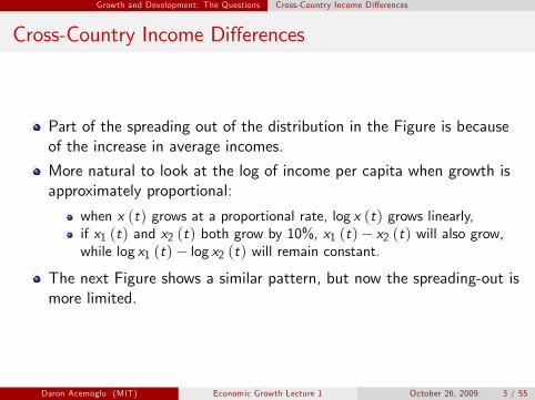
Part of the spreading out of the distribution in the Figure is because of the increase in average incomes.
More natural to look at the log of income per capita when growth is approximately proportional:
when x (t) grows at a proportional rate, log x (t) grows linearly, if x1 (t) and x2 (t) both grow by 10%, x1 (t) − x2 (t) will also grow, while log x1 (t) − log x2 (t) will remain constant.
The next Figure shows a similar pattern, but now the spreading-out is more limited.
Daron Acemoglu (MIT) Economic Growth Lecture 1 October 26, 2009. 3 / 55
Growth and Development: The Questions Cross-Country Income Differences
Cross-Country Income Differences
1960
1980
20000
.1.2
.3.4
Den
sity
of c
outri
es
6 7 8 9 10 11log gdp per capita
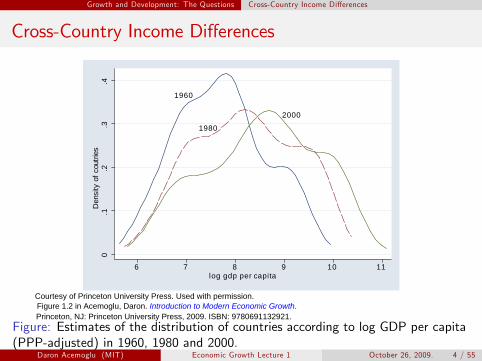
Courtesy of Princeton University Press. Used with permission.Figure 1.2 in Acemoglu, Daron. Introduction to Modern Economic Growth.Princeton, NJ: Princeton University Press, 2009. ISBN: 9780691132921.
Figure: Estimates of the distribution of countries according to log GDP per capita (PPP-adjusted) in 1960, 1980 and 2000.
Daron Acemoglu (MIT) Economic Growth Lecture 1 October 26, 2009. 4 / 55

1
2
Growth and Development: The Questions Cross-Country Income Differences
Cross-Country Income Differences
Theory is easier to map to data when we look at output (GDP) per worker.
Moreover, key sources of difference in economic performance across countries are national policies and institutions.
The next Figure looks at the unweighted distribution of countriesaccording to (PPP-adjusted) GDP per worker
“workers”: total economically active population according to the definition of the International Labour Organization.
Overall, two important facts:
Large amount of inequality in income per capita and income per worker across countries. Slight but noticeable increase in inequality across nations (though not necessarily across individuals in the entire world).
Daron Acemoglu (MIT) Economic Growth Lecture 1 October 26, 2009. 5 / 55

Growth and Development: The Questions Cross-Country Income Differences
Cross-Country Income Differences
1960
1980
2000
0.1
.2.3
.4D
ensit
y of
cou
tries
6 8 10 12log gdp per w orker
Courtesy of Princeton University Press. Used with permission. Figure 1.4 in Acemoglu, Daron. Introduction to Modern Economic Growth. Princeton, NJ: Princeton University Press, 2009. ISBN: 9780691132921.
Figure: Distribution of log GDP per worker (PPP-adjusted). Daron Acemoglu (MIT) Economic Growth Lecture 1 October 26, 2009. 6 / 55

Growth and Development: The Questions Economic Growth and Income Differences
Economic Growth and Income Differences
SpainSouth Korea
India
Brazil
USA
Singapore
Nigeria
Guatemala
UK
Botsw ana
67
89
10lo
g gd
p pe
r cap
ita
1960 1970 1980 1990 2000year
Courtesy of Princeton University Press. Used with permission. Figure 1.8 in Acemoglu, Daron. Introduction to Modern Economic Growth. Princeton, NJ: Princeton University Press, 2009. ISBN: 9780691132921.
Figure: The evolution of income per capita 1960-2000. Daron Acemoglu (MIT) Economic Growth Lecture 1 October 26, 2009. 7 / 55

Growth and Development: The Questions Economic Growth and Income Differences
Economic Growth and Income Differences
Why is the United States richer in 1960 than other nations and able to grow at a steady pace thereafter? How did Singapore, South Korea and Botswana manage to grow at a relatively rapid pace for 40 years? Why did Spain grow relatively rapidly for about 20 years, but thenslow down? Why did Brazil and Guatemala stagnate during the1980s?What is responsible for the disastrous growth performance of Nigeria?
Central questions for understanding how the capitalist system works and the origins of economic growth. Central questions also for policy and welfare, since differences in income related to living standards, consumption and health.
Our first task is to develop a coherent framework to investigate these questions and as a byproduct we will introduce the workhorse models of dynamic economic analysis and macroeconomics.
Daron Acemoglu (MIT) Economic Growth Lecture 1 October 26, 2009. 8 / 55

Growth and Development: The Questions Origins of Income Differences and World Economic Growth
Origins of Income Differences and World Growth
DZA
ARG
AUSAUT
BRB
BEL
BEN
BOL
BRA
BFA
BDI
CMR
CAN
CPV
TCD
CHL
CHN
COL
COMCOG
CRI
CIV
DNK
DOM
ECUEGY SLV
GNQ
ETH
FINFRA
GAB
GMB
GHA
GRC
GTM
GIN
GNB
HND
HKG ISL
IND
IDN
IRN
IRLISRITA
JAM
JPN
JOR
KEN
KOR
LSO
LUX
MDGMWI
MYS
MLI
MUS
MEX
MAR
MOZ
NPL
NLD
NZL
NIC
NER
NGA
NOR
PAK
PAN
PRYPER
PHL
PRT
ROM
RWA
SEN
SGP
ZAF
ESP
LKA
SWECHE
SYR
TZA
THA
TGO
TTO
TUR
UGA
GBR
USA
URY
VEN
ZMB
ZWE
.6.7
.8.9
11.
1lo
g G
DP
per
wor
ker r
elat
ive to
the
US
in 2
000
.6 .7 .8 .9 1log GDP per w orker relative to the US in 1960
Courtesy of Princeton University Press. Used with permission. Figure 1.9 in Acemoglu, Daron. Introduction to Modern Economic Growth. Princeton, NJ: Princeton University Press, 2009. ISBN: 9780691132921.
Figure: Log GDP per worker in 2000 and 1960. Daron Acemoglu (MIT) Economic Growth Lecture 1 October 26, 2009. 9 / 55

..
Growth and Development: The Questions Origins of Income Differences and World Economic Growth
Origins of Income Differences and World Growth
Western Of f shoots
Western Europe
Af ricaLatin America
Asia
67
89
10lo
g gd
p pe
r cap
ita
1800 1850 1900 1950 2000year
Courtesy of Princeton University Press. Used with permission.Figure 1.10 in Acemoglu, Daron. Introduction to Modern Economic Growth Princeton, NJ: Princeton University Press, 2009. ISBN: 9780691132921.
Figure: Evolution of GDP per capita 1820-2000. Daron Acemoglu (MIT) Economic Growth Lecture 1 October 26, 2009. 10 / 55

.
Growth and Development: The Questions Origins of Income Differences and World Economic Growth
Origins of Income Differences and World Growth
Western Of f shoots
Western Europe
Af rica
LatinAmerica
Asia
67
89
10lo
g gd
p pe
r cap
ita
1000 1200 1400 1600 1800 2000year
Courtesy of Princeton University Press. Used with permission. Figure 1.11 in Acemoglu, Daron. Introduction to Modern Economic GrowthPrinceton, NJ: Princeton University Press, 2009. ISBN: 9780691132921.
Figure: Evolution of GDP 1000-2000. Daron Acemoglu (MIT) Economic Growth Lecture 1 October 26, 2009. 11 / 55
.

Growth and Development: The Questions Origins of Income Differences and World Economic Growth
Origins of Income Differences and World Growth
USA
Britain
Spain
Ghana
Brazil
China
India
67
89
10lo
g gd
p pe
r cap
ita
1800 1850 1900 1950 2000year
Courtesy of Princeton University Press. Used with permission. Figure 1.12 in Acemoglu, Daron. Introduction to Modern Economic Growth. Princeton, NJ: Princeton University Press, 2009. ISBN: 9780691132921.Figure: Evolution of income per capita in various countries.
Daron Acemoglu (MIT) Economic Growth Lecture 1 October 26, 2009. 12 / 55

Growth and Development: The Questions Correlates of Economic Growth
Correlates of Economic Growth
ARG
AUS
AUTBEL
BENBOL
BRA
BFA
CANCHL
CHN
COLCRI
DNK
DOM
ECU
EGY
SLV
ETH
FINFRA
GHA
GRC
GTM
GIN
HND
ISLIND
IRN
IRL
ISRITA
JAM
JPN
JOR
KEN
KOR
LUX
MWI
MYS
MUS
MEX
MAR NLD
NZL
NIC
NGA
NOR
PAK
PAN
PRY
PER
PHL
PRT
ZAF
ESPLKA
SWE
CHE
TWN
THA
TTOTUR
UGA
GBRUSA
URY
VENZMB
ZWE
0.0
2.0
4.0
6.0
8Av
erag
e G
row
th R
ate
of G
DP
per
Cap
ita 1
960
2000
0 .1 .2 .3 .4Average Investment Rate 19602000
Courtesy of Princeton University Press. Used with permission.Figure 1.15 in Acemoglu, Daron. Introduction to Modern Economic Growth. Princeton, NJ: Princeton University Press, 2009. ISBN: 9780691132921.
Figure: Average investment to GDP ratio and economic growth. Daron Acemoglu (MIT) Economic Growth Lecture 1 October 26, 2009. 13 / 55

Growth and Development: The Questions Correlates of Economic Growth
Correlates of Economic Growth
ARG
AUS
AUT
BDI
BEL
BEN
BOL
BRA
BRBCAN
CHECHL
CHN
CMRCOG
COLCRI
DNKDOM
DZA
ECU
EGY
ESP
FINFRA
GBR
GHA
GMB
GRC
GTM
HKG
HND
IDNIND
IRL
IRN
ISL
ISRITA
JAM
JOR
JPN
KEN
KOR
LKALSO
MEXMLIMOZ
MUS
MWI
MYS
NER
NIC
NLD
NOR
NPL
NZL
PAK
PAN
PER
PHL
PRT
PRY
RWASEN
SGP
SLV
SWE
SYR
TGO
THA
TTO
TUN TUR
TWN
UGA
URY
USA
VEN
ZAF
ZMB
ZWE
.02
0.0
2.0
4.0
6Av
erag
e G
row
th R
ate
of G
DP
per
Cap
ita 1
960
2000
0 2 4 6 8 10 12Average Years of Schooling 19602000
Courtesy of Princeton University Press. Used with permission. Figure 1.16 in Acemoglu, Daron. Introduction to Modern Economic Growth. Princeton, NJ: Princeton University Press, 2009. ISBN: 9780691132921.
Figure: Schooling and economic growth. Daron Acemoglu (MIT) Economic Growth Lecture 1 October 26, 2009. 14 / 55

Growth and Development: The Questions From Correlates to Fundamental Causes
From Correlates to Fundamental Causes
Correlates of economic growth, such as physical capital, human capital and technology, will be our first topic of study. But these are only proximate causes of economic growth and economic success:
why do certain societies fail to improve their technologies, invest more in physical capital, and accumulate more human capital?
Return to Figure above to illustrate this point further:
how did South Korea and Singapore manage to grow, while Nigeria failed to take advantage of the growth opportunities? If physical capital accumulation is so important, why did Nigeria not invest more in physical capital? If education is so important, why our education levels in Nigeria still so low and why is existing human capital not being used more effectively?
The answer to these questions is related to the fundamental causes of economic growth.
Daron Acemoglu (MIT) Economic Growth Lecture 1 October 26, 2009. 15 / 55

1
2
3
4
Growth and Development: The Questions From Correlates to Fundamental Causes
From Correlates to Fundamental Causes
We can think of the following list of potential fundamental causes:
luck (or multiple equilibria) geographic differences institutional differences cultural differences
An important caveat should be noted: discussions of geography, institutions and culture can sometimes be carried out without explicit reference to growth models or even to growth empirics. But it is only by formulating parsimonious models of economic growth and confronting them with data that we can gain a better understanding of both the proximate and the fundamental causes of economic growth.
Daron Acemoglu (MIT) Economic Growth Lecture 1 October 26, 2009. 16 / 55

Solow Growth Model Solow Growth Model
Solow Growth Model
Develop a simple framework for the proximate causes and the mechanics of economic growth and cross-country income differences.
Solow-Swan model named after Robert (Bob) Solow and Trevor Swan, or simply the Solow model
Before Solow growth model, the most common approach to economic growth built on the Harrod-Domar model.
Harrod-Domar mdel emphasized potential dysfunctional aspects of growth: e.g, how growth could go hand-in-hand with increasing unemployment.
Solow model demonstrated why the Harrod-Domar model was not an attractive place to start.
At the center of the Solow growth model is the neoclassical aggregate production function.
Daron Acemoglu (MIT) Economic Growth Lecture 1 October 26, 2009. 17 / 55

Solow Growth Model The Economic Environment of the Basic Solow Model
The Economic Environment of the Basic Solow Model
Study of economic growth and development therefore necessitates dynamic models.
Despite its simplicity, the Solow growth model is a dynamic general equilibrium model (though many key features of dynamic general equilibrium models, such as preferences and dynamic optimization are missing in this model).
Daron Acemoglu (MIT) Economic Growth Lecture 1 October 26, 2009. 18 / 55

Solow Growth Model Households and Production
Households and Production I
Closed economy, with a unique final good.
Discrete time running to an infinite horizon, time is indexed by t = 0, 1, 2, ....
Economy is inhabited by a large number of households, and for now households will not be optimizing.
This is the main difference between the Solow model and the neoclassical growth model.
To fix ideas, assume all households are identical, so the economy admits a representative household.
Daron Acemoglu (MIT) Economic Growth Lecture 1 October 26, 2009. 19 / 55

Solow Growth Model Households and Production
Households and Production II
Assume households save a constant exogenous fraction s of their disposable income Same assumption used in basic Keynesian models and in the Harrod-Domar model; at odds with reality. Assume all firms have access to the same production function: economy admits a representative firm, with a representative (or aggregate) production function. Aggregate production function for the unique final good is
Y (t) = F [K (t) , L (t) , A (t)] (1)
Assume capital is the same as the final good of the economy, but used in the production process of more goods. A (t) is a shifter of the production function (1). Broad notion of technology. Major assumption: technology is free; it is publicly available as a non-excludable, non-rival good.
Daron Acemoglu (MIT) Economic Growth Lecture 1 October 26, 2009. 20 / 55

Solow Growth Model Households and Production
Key Assumption
Assumption 1 (Continuity, Differentiability, Positive and Diminishing Marginal Products, and Constant Returns to Scale) The production function F : R3 R+ is twice continuously + →differentiable in K and L, and satisfies
FK (K , L, A) ≡ ∂F (·)
> 0, FL(K , L, A) ≡ ∂F (·)
> 0,∂K ∂L
FKK (K , L, A) ≡ ∂2
∂
FK (2
·) < 0, FLL (K , L, A) ≡
∂2
∂
FL(2
·) < 0.
Moreover, F exhibits constant returns to scale in K and L.
Assume F exhibits constant returns to scale in K and L. I.e., it is linearly homogeneous (homogeneous of degree 1) in these two variables.
Daron Acemoglu (MIT) Economic Growth Lecture 1 October 26, 2009. 21 / 55

Solow Growth Model Households and Production
Review
Definition Let K be an integer. The function g : RK +2 R is→homogeneous of degree m in x ∈ R and y ∈ R if and only if
g (λx , λy , z) = λmg (x , y , z) for all λ ∈ R+ and z ∈ RK .
Theorem (Euler’s Theorem) Suppose that g : RK +2 R is→continuously differentiable in x ∈ R and y ∈ R, with partial derivatives denoted by gx and gy and is homogeneous of degree m in x and y . Then
mg (x , y , z) = gx (x , y , z) x + gy (x , y , z) y
for all x ∈ R, y ∈ R and z ∈ RK .
Moreover, gx (x , y , z) and gy (x , y , z) are themselves homogeneous of degree m − 1 in x and y .
Daron Acemoglu (MIT) Economic Growth Lecture 1 October 26, 2009. 22 / 55

Solow Growth Model Market Structure, Endowments and Market Clearing
Market Structure, Endowments and Market Clearing I
We will assume that markets are competitive, so ours will be a prototypical competitive general equilibrium model. Households own all of the labor, which they supply inelastically. Endowment of labor in the economy, L̄ (t), and all of this will be supplied regardless of the price. The labor market clearing condition can then be expressed as:
L (t) =L̄ (t) (2)
for all t, where L (t) denotes the demand for labor (and also the level of employment). More generally, should be written in complementary slackness form. In particular, let the wage rate at time t be w (t), then the labor market clearing condition takes the form
L (t) ≤L̄ (t) , w (t) ≥ 0 and (L (t) − L̄ (t)) w (t) = 0
Daron Acemoglu (MIT) Economic Growth Lecture 1 October 26, 2009. 23 / 55

Solow Growth Model Market Structure, Endowments and Market Clearing
Market Structure, Endowments and Market Clearing II
But Assumption 1 and competitive labor markets make sure that wages have to be strictly positive.
Households also own the capital stock of the economy and rent it to firms.
Denote the rental price of capital at time t be R (t).
Capital market clearing condition:
Ks (t) = Kd (t)
Take households’initial holdings of capital, K (0), as given
P (t) is the price of the final good at time t, normalize the price of the final good to 1 in all periods.
Build on an insight by Kenneth Arrow (Arrow, 1964) that it is suffi cient to price securities (assets) that transfer one unit of consumption from one date (or state of the world) to another.
Daron Acemoglu (MIT) Economic Growth Lecture 1 October 26, 2009. 24 / 55

Solow Growth Model Market Structure, Endowments and Market Clearing
Market Structure, Endowments and Market Clearing III
Implies that we need to keep track of an interest rate across periods, r (t), and this will enable us to normalize the price of the final good to 1 in every period.
General equilibrium economies, where different commodities correspond to the same good at different dates.
The same good at different dates (or in different states or localities)is a different commodity.
Therefore, there will be an infinite number of commodities.
Assume capital depreciates, with “exponential form,” at the rate δ:out of 1 unit of capital this period, only 1 − δ is left for next period.
Loss of part of the capital stock affects the interest rate (rate ofreturn to savings) faced by the household.
Interest rate faced by the household will be r (t) = R (t) − δ.
Daron Acemoglu (MIT) Economic Growth Lecture 1 October 26, 2009. 25 / 55

1
2
3
4
Solow Growth Model Firm Optimization
Firm Optimization I
Only need to consider the problem of a representative firm:
max F [K (t), L(t), A(t)] − w (t) L (t) − R (t) K (t) . (3)L(t)≥0,K (t)≥0
Since there are no irreversible investments or costs of adjustments, the production side can be represented as a static maximization problem.
Equivalently, cost minimization problem.
Features worth noting:
Problem is set up in terms of aggregate variables. Nothing multiplying the F term, price of the final good has normalized to 1. Already imposes competitive factor markets: firm is taking as given w (t) and R (t). Concave problem, since F is concave.
Daron Acemoglu (MIT) Economic Growth Lecture 1 October 26, 2009. 26 / 55

Solow Growth Model Firm Optimization
Firm Optimization II
Since F is differentiable, first-order necessary conditions imply:
w (t) = FL[K (t), L(t), A(t)], (4)
and R (t) = FK [K (t), L(t), A(t)]. (5)
Note also that in (4) and (5), we used K (t) and L (t), the amount of capital and labor used by firms.
In fact, solving for K (t) and L (t), we can derive the capital and labor demands of firms in this economy at rental prices R (t) and w (t).
Thus we could have used Kd (t) instead of K (t), but this additional notation is not necessary.
Daron Acemoglu (MIT) Economic Growth Lecture 1 October 26, 2009. 27 / 55

Solow Growth Model Firm Optimization
Firm Optimization III
Proposition Suppose Assumption 1 holds. Then in the equilibrium of the Solow growth model, firms make no profits, and in particular,
Y (t) = w (t) L (t) + R (t) K (t) .
Proof: Follows immediately from Euler Theorem for the case of m = 1, i.e., constant returns to scale.
Thus firms make no profits, so ownership of firms does not need to be specified.
Daron Acemoglu (MIT) Economic Growth Lecture 1 October 26, 2009. 28 / 55

Solow Growth Model Firm Optimization
Second Key Assumption
Assumption 2 (Inada conditions) F satisfies the Inada conditions
lim FK ( ) = ∞ and lim FK ( ) = 0 for all L > 0 all A K 0
·K ∞
·→ →
Llim0 FL (·) = ∞ and
Llim
∞ FL (·) = 0 for all K > 0 all A.
→ →
Important in ensuring the existence of interior equilibria.
It can be relaxed quite a bit, though useful to get us started.
Daron Acemoglu (MIT) Economic Growth Lecture 1 October 26, 2009. 29 / 55

Solow Growth Model Firm Optimization
Production Functions
F(K, L, A)
K0
K0
Panel A Panel B
F(K, L, A)
Courtesy of Princeton University Press. Used with permission.
Figure 2.1 in Acemoglu, Daron. Introduction to Modern Economic Growth. Princeton, NJ: Princeton University Press, 2009. ISBN: 9780691132921.
Figure: Production functions and the marginal product of capital. The example in Panel A satisfies the Inada conditions in Assumption 2, while the example in Panel B does not.
Daron Acemoglu (MIT) Economic Growth Lecture 1 October 26, 2009. 30 / 55

The Solow Model in Discrete Time Fundamental Law of Motion of the Solow Model
Fundamental Law of Motion of the Solow Model I
Recall that K depreciates exponentially at the rate δ, so
K (t + 1) = (1 − δ) K (t) + I (t) , (6)
where I (t) is investment at time t. From national income accounting for a closed economy,
Y (t) = C (t) + I (t) , (7)
Using (1), (6) and (7), any feasible dynamic allocation in this economy must satisfy
K (t + 1) ≤ F [K (t) , L (t) , A (t)] + (1 − δ) K (t) − C (t)
for t = 0, 1, .... Behavioral rule of the constant saving rate simplifies the structure of equilibrium considerably.
Daron Acemoglu (MIT) Economic Growth Lecture 1 October 26, 2009. 31 / 55

The Solow Model in Discrete Time Fundamental Law of Motion of the Solow Model
Fundamental Law of Motion of the Solow Model II
Note not derived from the maximization of utility function: welfare comparisons have to be taken with a grain of salt.
Since the economy is closed (and there is no government spending),
S (t) = I (t) = Y (t) − C (t) .
Individuals are assumed to save a constant fraction s of their income,
S (t) = sY (t) , (8)
C (t) = (1 − s) Y (t) (9)
Implies that the supply of capital resulting from households’behavior can be expressed as
Ks (t) = (1 − δ)K (t) + S (t) = (1 − δ)K (t) + sY (t) .
Daron Acemoglu (MIT) Economic Growth Lecture 1 October 26, 2009. 32 / 55

The Solow Model in Discrete Time Fundamental Law of Motion of the Solow Model
Fundamental Law of Motion of the Solow Model III
Setting supply and demand equal to each other, this implies Ks (t) = K (t).
From (2), we have L (t) = L̄ (t).
Combining these market clearing conditions with (1) and (6), we obtain the fundamental law of motion the Solow growth model:
K (t + 1) = sF [K (t) , L (t) , A (t)] + (1 − δ) K (t) . (10)
Nonlinear difference equation.
Equilibrium of the Solow growth model is described by this equation together with laws of motion for L (t) (or L̄ (t)) and A (t).
Daron Acemoglu (MIT) Economic Growth Lecture 1 October 26, 2009. 33 / 55

The Solow Model in Discrete Time Definition of Equilibrium
Definition of Equilibrium I
Solow model is a mixture of an old-style Keynesian model and a modern dynamic macroeconomic model.
Households do not optimize, but firms still maximize and factor markets clear.
Definition In the basic Solow model for a given sequence of{L (t) , A (t)} ∞
=0 and an initial capital stock K (0), ant equilibrium path is a sequence of capital stocks, output levels, consumption levels, wages and rental rates{K (t) , Y (t) , C (t) , w (t) , R (t)} ∞
=0 such that K (t)t satisfies (10), Y (t) is given by (1), C (t) is given by (9), and w (t) and R (t) are given by (4) and (5).
Note an equilibrium is defined as an entire path of allocations and prices: not a static object.
Daron Acemoglu (MIT) Economic Growth Lecture 1 October 26, 2009. 34 / 55

1
2
The Solow Model in Discrete Time Equilibrium
Equilibrium Without Population Growth and Technological Progress I
Make some further assumptions, which will be relaxed later: There is no population growth; total population is constant at some level L > 0. Since individuals supply labor inelastically, L (t) = L. No technological progress, so that A (t) = A.
Define the capital-labor ratio of the economy as
k (t) ≡ K (t)
, (11)L
Using the constant returns to scale assumption, we can express output (income) per capita, y (t) ≡ Y (t) /L, as
y (t) = � � K (t)
F , 1, AL
≡ f (k (t)) . (12)
Daron Acemoglu (MIT) Economic Growth Lecture 1 October 26, 2009. 35 / 55

The Solow Model in Discrete Time Equilibrium
Equilibrium Without Population Growth and Technological Progress II
Note that f (k) here depends on A, so I could have written f (k, A); but A is constant and can be normalized to A = 1.
From Euler Theorem,
R (t) = f � (k (t)) > 0 and
w (t) = f (k (t)) − k (t) f � (k (t)) > 0. (13)
Both are positive from Assumption 1.
Daron Acemoglu (MIT) Economic Growth Lecture 1 October 26, 2009. 36 / 55

The Solow Model in Discrete Time Equilibrium
Example:The Cobb-Douglas Production Function I
Very special production function and many interesting phenomena are ruled out, but widely used:
Y (t) = F [K (t) , L (t) , A (t)]
= AK (t)α L (t)1−α , 0 < α < 1. (14)
Satisfies Assumptions 1 and 2. Dividing both sides by L (t),
y (t) = Ak (t)α ,
From equation (13),
∂Ak (t)α
R (t) = ,∂k (t)
= αAk (t)−(1−α) .
Daron Acemoglu (MIT) Economic Growth Lecture 1 October 26, 2009. 37 / 55
The Solow Model in Discrete Time Equilibrium
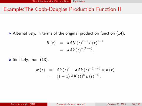
Example:The Cobb-Douglas Production Function II
Alternatively, in terms of the original production function (14),
R (t) = αAK (t)α−1 L (t)1−α
= αAk (t)−(1−α) ,
Similarly, from (13),
w (t) = Ak (t)α − αAk (t)−(1−α) × k (t)
= (1 − α) AK (t)α L (t)−α ,
Daron Acemoglu (MIT) Economic Growth Lecture 1 October 26, 2009. 38 / 55

The Solow Model in Discrete Time Equilibrium
Equilibrium Without Population Growth and Technological Progress I
The per capita representation of the aggregate production function enables us to divide both sides of (10) by L to obtain:
k (t + 1) = sf (k (t)) + (1 − δ) k (t) . (15)
Since it is derived from (10), it also can be referred to as the equilibrium difference equation of the Solow model The other equilibrium quantities can be obtained from the capital-labor ratio k (t).
Definition A steady-state equilibrium without technological progress and population growth is an equilibrium path in which k (t) = k∗ for all t.
The economy will tend to this steady state equilibrium over time (but never reach it in finite time).
Daron Acemoglu (MIT) Economic Growth Lecture 1 October 26, 2009. 39 / 55

k(t+1)
k(t)
45°
sf(k(t))+(1–δ)k(t)k*
k*0
The Solow Model in Discrete Time Equilibrium
Courtesy of Princeton University Press. Used with permission.Figure 2.2 in Acemoglu, Daron. Introduction to Modern Economic Growth.
Princeton, NJ: Princeton University Press, 2009. ISBN: 9780691132921.
Figure: Determination of the steady-state capital-labor ratio in the Solow model without population growth and technological change.
Daron Acemoglu (MIT) Economic Growth Lecture 1 October 26, 2009. 40 / 55

1
2
3
The Solow Model in Discrete Time Equilibrium
Equilibrium Without Population Growth and Technological Progress II
Thick curve represents (15) and the dashed line corresponds to the 45◦ line.
Their (positive) intersection gives the steady-state value of the capital-labor ratio k∗,
f (k∗) δ = . (16)
k∗ s There is another intersection at k = 0, because the figure assumes that f (0) = 0.
Will ignore this intersection throughout:
If capital is not essential, f (0) will be positive and k = 0 will cease tobe a steady state equilibrium This intersection, even when it exists, is an unstable point It has no economic interest for us.
Daron Acemoglu (MIT) Economic Growth Lecture 1 October 26, 2009. 41 / 55

Figure: Unique steady state in the basic Solow model when f (0) = ε > 0.
The Solow Model in Discrete Time Equilibrium
Equilibrium Without Population Growth and Technological Progress III
k(t+1)
k(t)
45°
k*
k*
ε
sf(k(t))+(1−δ)k(t)
0Daron Acemoglu (MIT) Economic Growth Lecture 1 October 26, 2009. 42 / 55
Courtesy of Princeton University Press. Used with permission. Figure 2.3 in Acemoglu, Daron. Introduction to Modern Economic Growth. Princeton, NJ: Princeton University Press, 2009. ISBN: 9780691132921.

1
2
The Solow Model in Discrete Time Equilibrium
Equilibrium Without Population Growth and Technological Progress IV
Alternative visual representation of the steady state: intersection between δk and the function sf (k). Useful because:
Depicts the levels of consumption and investment in a single figure. Emphasizes the steady-state equilibrium sets investment, sf (k), equal to the amount of capital that needs to be “replenished”, δk.
Daron Acemoglu (MIT) Economic Growth Lecture 1 October 26, 2009. 43 / 55

The Solow Model in Discrete Time Equilibrium
output
k(t)
f(k*)
k*
δk(t)
f(k(t))
sf(k*)sf(k(t))
consumption
investment
0Courtesy of Princeton University Press. Used with permission. Figure 2.4 in Acemoglu, Daron. Introduction to Modern Economic Growth.Princeton, NJ: Princeton University Press, 2009. ISBN: 9780691132921.
Figure: Investment and consumption in the steady-state equilibrium. Daron Acemoglu (MIT) Economic Growth Lecture 1 October 26, 2009. 44 / 55

The Solow Model in Discrete Time Equilibrium
Equilibrium Without Population Growth and Technological Progress V
Proposition Consider the basic Solow growth model and suppose that Assumptions 1 and 2 hold. Then there exists a unique steady state equilibrium where the capital-labor ratio k∗ ∈ (0, ∞) is given by (16), per capita output is given by
y ∗ = f (k∗) (17)
and per capita consumption is given by
c∗ = (1 − s) f (k∗) . (18)
Daron Acemoglu (MIT) Economic Growth Lecture 1 October 26, 2009. 45 / 55

The Solow Model in Discrete Time Equilibrium
Proof of Theorem
The preceding argument establishes that any k∗ that satisfies (16) is a steady state.
To establish existence, note that from Assumption 2 (and from L’Hospital’s rule), limk 0 f (k) /k = ∞ and limk ∞ f (k) /k = 0. → →
Moreover, f (k) /k is continuous from Assumption 1, so by the Intermediate Value Theorem there exists k∗ such that (16) is satisfied.
To see uniqueness, differentiate f (k) /k with respect to k, whichgives
∂ [f (k) /k ] f w =
� (k) kk2− f (k)
= − k2 < 0, (19)
∂k where the last equality uses (13).
Since f (k) /k is everywhere (strictly) decreasing, there can only exist a unique value k∗ that satisfies (16).
Equations (17) and (18) then follow by definition.
Daron Acemoglu (MIT) Economic Growth Lecture 1 October 26, 2009. 46 / 55

The Solow Model in Discrete Time Equilibrium
k(t+1)
k(t)
45°
sf(k(t))+(1–δ)k(t)
0
k(t+1)
k(t)
45°
sf(k(t))+(1–δ)k(t)
0
k(t+1)
k(t)
45°
sf(k(t))+(1–δ)k(t)
0
0Panel A Panel B Panel C
Courtesy of Princeton University Press. Used with permission. Figure 2.5 in Acemoglu, Daron. Introduction to Modern Economic Growth. Princeton, NJ: Princeton University Press, 2009. ISBN: 9780691132921.
Figure: Examples of nonexistence and nonuniqueness of interior steady stateswhen Assumptions 1 and 2 are not satisfied.
Daron Acemoglu (MIT) Economic Growth Lecture 1 October 26, 2009. 47 / 55
The Solow Model in Discrete Time Equilibrium
Equilibrium Without Population Growth and Technological Progress VI
Figure shows through a series of examples why Assumptions 1 and 2 cannot be dispensed with for the existence and uniqueness results.
Generalize the production function in one simple way, and assume that
f (k) = af̃ (k) ,
a > 0, so that a is a (“Hicks-neutral”) shift parameter, with greater values corresponding to greater productivity of factors..
Since f (k) satisfies the regularity conditions imposed above, so does f̃ (k).
Daron Acemoglu (MIT) Economic Growth Lecture 1 October 26, 2009. 48 / 55

The Solow Model in Discrete Time Equilibrium
Equilibrium Without Population Growth and Technological Progress VII
Proposition Suppose Assumptions 1 and 2 hold and f (k) = af̃ (k). Denote the steady-state level of the capital-labor ratio by k∗ (a, s, δ) and the steady-state level of output by y ∗ (a, s, δ) when the underlying parameters are a, s and δ. Then we have
∂k∗ ( ) ∂k∗ ( ) ∂k∗ ( )·> 0,
·> 0 and
·< 0
∂a ∂s ∂δ ∂y ∗ ( ) ∂y ∗ ( ) ∂y ∗ ( )·
> 0, ·> 0 and
·< 0.
∂a ∂s ∂δ
Daron Acemoglu (MIT) Economic Growth Lecture 1 October 26, 2009. 49 / 55

The Solow Model in Discrete Time Equilibrium
Equilibrium Without Population Growth and Technological Progress VIII
Proof of comparative static results: follows immediately by writing
f̃ (k∗) δ k∗
= as ,
which holds for an open set of values of k∗. Now apply the implicit function theorem to obtain the results.
For example, ∂k∗ δ (k∗)2
= > 0 ∂s s2w ∗
where w ∗ = f (k∗) − k∗f � (k∗) > 0.
The other results follow similarly.
Daron Acemoglu (MIT) Economic Growth Lecture 1 October 26, 2009. 50 / 55

The Solow Model in Discrete Time Equilibrium
Equilibrium Without Population Growth and Technological Progress IX
Same comparative statics with respect to a and δ immediately apply to c∗ as well. But c∗ will not be monotone in the saving rate (think, for example, of s = 1). In fact, there will exist a specific level of the saving rate, sgold , referred to as the “golden rule” saving rate, which maximizes c∗. But cannot say whether the golden rule saving rate is “better” than some other saving rate. Write the steady state relationship between c∗ and s and suppress the other parameters:
c∗ (s) = (1 − s) f (k∗ (s)) ,
= f (k∗ (s)) − δk∗ (s) ,
The second equality exploits that in steady state sf (k) = δk.
Daron Acemoglu (MIT) Economic Growth Lecture 1 October 26, 2009. 51 / 55

� �
The Solow Model in Discrete Time Equilibrium
Equilibrium Without Population Growth and Technological Progress X
Differentiating with respect to s,
∂c∗ (s) � � ∂k∗ = f � (k∗ (s)) − δ . (20)
∂s ∂s
sgold is such that ∂c∗ (sgold ) /∂s = 0. The corresponding steady-state golden rule capital stock is defined as k∗ gold .
Proposition In the basic Solow growth model, the highest level of steady-state consumption is reached for sgold , with the corresponding steady state capital level k∗
gold such that
f k∗ = δ. (21)� gold
Daron Acemoglu (MIT) Economic Growth Lecture 1 October 26, 2009. 52 / 55

The Solow Model in Discrete Time Equilibrium
consumption
savings rate
(1–s)f(k*gold)
s*gold 10
Courtesy of Princeton University Press. Used with permission.Figure 2.6 in Acemoglu, Daron. Introduction to Modern Economic Growth.Princeton, NJ: Princeton University Press, 2009. ISBN: 9780691132921.
Figure: The “golden rule” level of savings rate, which maximizes steady-state consumption.
Daron Acemoglu (MIT) Economic Growth Lecture 1 October 26, 2009. 53 / 55

The Solow Model in Discrete Time Equilibrium
Proof of Proposition: Golden Rule
By definition ∂c∗ (sgold ) /∂s = 0.
From Proposition above, ∂k∗/∂s > 0, thus (20) can be equal to zero only when f � (k∗ (sgold )) = δ.
Moreover, when f � (k∗ (sgold )) = δ, it can be verified that ∂2c∗ (sgold ) /∂s2 < 0, so f � (k∗ (sgold )) = δ indeed corresponds a local maximum.
That f � (k∗ (sgold )) = δ also yields the global maximum is a consequence of the following observations:
∀ s ∈ [0, 1] we have ∂k∗/∂s > 0 and moreover, when s < sgold ,f � (k∗ (s)) − δ > 0 by the concavity of f , so ∂c∗ (s) /∂s > 0 for alls < sgold .by the converse argument, ∂c∗ (s) /∂s < 0 for all s > sgold .Therefore, only sgold satisfies f � (k∗ (s)) = δ and gives the uniqueglobal maximum of consumption per capita.
Daron Acemoglu (MIT) Economic Growth Lecture 1 October 26, 2009. 54 / 55

The Solow Model in Discrete Time Equilibrium
Equilibrium Without Population Growth and Technological Progress XI
When the economy is below k∗ gold , higher saving will increase consumption; when it is above k∗ gold , steady-state consumption can be increased by saving less.
In the latter case, capital-labor ratio is too high so that individuals are investing too much and not consuming enough (dynamic ineffi ciency).
But no utility function, so statements about “ineffi ciency” have to be considered with caution.
Such dynamic ineffi ciency will not arise once we endogenize consumption-saving decisions.
Daron Acemoglu (MIT) Economic Growth Lecture 1 October 26, 2009. 55 / 55

For information about citing these materials or our Terms of Use, visit: http://ocw.mit.edu/terms.
MIT OpenCourseWare http://ocw.mit.edu
14.452 Economic Growth Fall 2009
For information about citing these materials or our Terms of Use,visit: http://ocw.mit.edu/terms.
Top Related