


Languages
Pages
Legal

1
Part I: Blade Design Methods and Issues
James L. Tangler
Senior Scientist
Steady-State Aerodynamics Codes for HAWTsSelig, Tangler, and Giguère
August 2, 1999 NREL NWTC, Golden, CO
National Renewable Energy LaboratoryNational Wind Technology Center
2
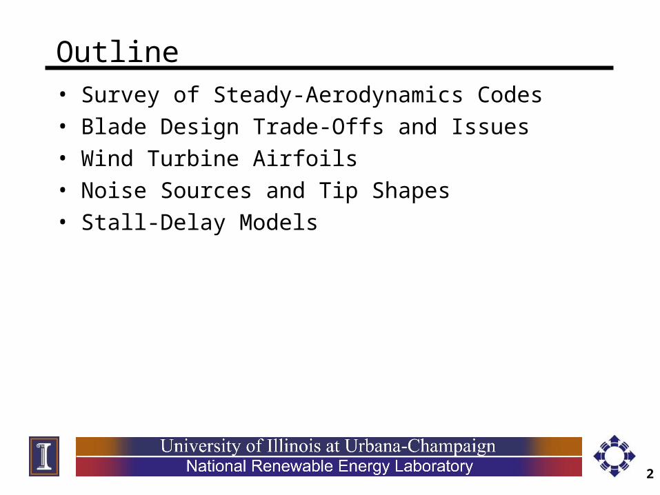
Outline• Survey of Steady-Aerodynamics Codes• Blade Design Trade-Offs and Issues• Wind Turbine Airfoils• Noise Sources and Tip Shapes• Stall-Delay Models

3
Survey of Steady-Aerodynamics Codes• Historical Development of BEMT Performance and Design Methods in the US
– Summary
Year Codes Developers
1974 PROP Wilson and Walker
1981 WIND Snyder
1983 Revised PROP Hibbs and Radkey PROPSH Tangler WIND-II Snyder and Staples
1984 PROPFILE Fairbank and Rogers

4
Year Code Developer
1986 NUPROP Hibbs
1987 PROPPC Kocurek
1993 PROP93 McCarty
1994 PROPID Selig
1995 WIND-III Huang and MillerPROPGA Selig and Coverstone-Carroll
1996 WT_PERF Buhl
1998 PROP98 Combs
2000 New PROPGA Giguère

5
PROP1974– Fortran 77
WIND1981– Based on PROP code– Accounts for spoilers,
ailerons, and other airfoilmodifications
Revised PROP1983– Windmill brake state– Wind shear effects– Flat-plate post-stall
airfoil characteristics
– Some details of each code
6
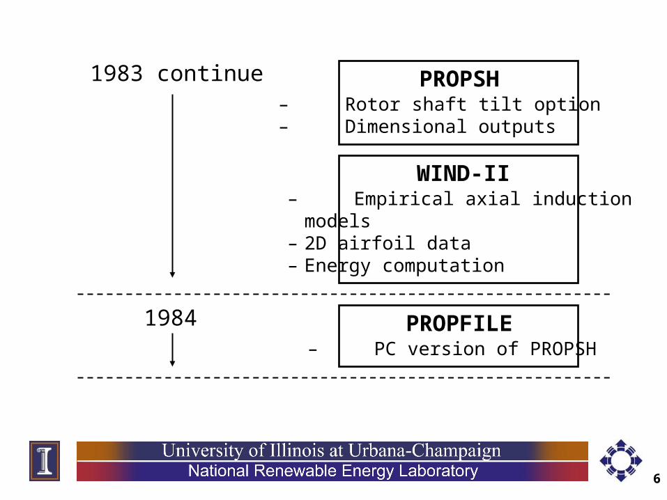
1983 continue
PROPFILE1984– PC version of PROPSH
WIND-II– Empirical axial induction
models– 2D airfoil data– Energy computation
PROPSH– Rotor shaft tilt option– Dimensional outputs

7
NUPROP1986– Dynamic stall– Wind shear– Tower shadow– Yaw error– Large scale turbulence
PROPPC1987– PC version of PROP
PROP931993– PROP with graphical
outputs– Programmed in C
8
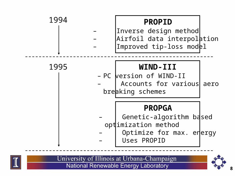
PROPID1994– Inverse design method– Airfoil data interpolation– Improved tip-loss model
WIND-III1995– PC version of WIND-II– Accounts for various aero
breaking schemes
PROPGA– Genetic-algorithm based
optimization method– Optimize for max. energy– Uses PROPID

9
WT_PERF1996
– Improved tip-loss model– Drag term in calculating
inplane induced velocities– Fortran 90
PROP981998– Enhanced graphics – Windows Interface
New PROPGA2000– Structural and cost
considerations– Airfoil selection– Advanced GA operators– Multi objectives

10
• Types of Steady-State BEMT Performance and Design Methods
Analysis Inverse Design OptimizationPROP PROPID PROPGAWIND Revised PROP PROPSHWIND-IIPROPFILENUPROPPROPPCPROP93WIND-IIIWT_PERFPROP98

11
CODES PROPPCWT-Perf
NUPROP PROP93 PROPID
Features AeroVironmentNREL
AeroVironment AEI Univ. of Illinois
Development Date 1987 1986 1993 1997Airfoil Data Interpolation no no no yes3-D Stall Delay no no no yesGlauert Approximation yes yes yes yesTip Losses yes yes yes yesWindspeed Sweep yes yes yes yesPitch Sweep yes yes yes yesShaft Tilt yes yes yes yesYaw Angle no yes yes yesTower Shadow no yes no yesDynamic Stall no yes no noGraphics no no yes noProgram Language Fortran Fortran C FortranOther turbulence hub ext. Inverse designCost free free $50 free
• Features of Selected Performance and Design Codes

12
• Glauert Correction for the Viscous Interaction– less induced velocity– greater angle of attack– more thrust and power

13
• Prediction Sources of Error– Airfoil data
• Correct Reynolds number• Post-stall characteristics
– Tip-loss model– Generator slip RPM change

14
• How Is Lift and Drag Used?– Only lift used to calculate the axial induction factor a– Both lift and drag used to calculate the swirl a’

15
• Designing for Steady-State Performance vs Performance in Stochastic Wind Environment– Turbulence – Wind shear– Dynamic stall– Yaw error– Elastic twist– Blade roughness

16
Blade Design Trade-offs and Issues• Aerodynamics vs Stuctures vs Dynamics vs Cost
– The aerodynamicists desire thin airfoils for low drag and minimum roughness sensitivity– The structural designers desire thick airfoils for stiffness and light weight
– The dynamicists desires depend on the turbine configuration but often prefer airfoils with a soft stall, which typically have a low to moderate Clmax
– The accountant wants low blade solidity from high Clmax airfoils, which typically leads to lower blade weight and cost

17
• Low-Lift vs High-Lift Airfoils– Low-lift implies larger blade solidity, and thus larger extreme loads– Extreme loads particularly important for large wind turbines– Low-lift airfoils have typically a soft stall, which is dynamically beneficial, and reduce power spikes – High-lift implies smaller chord lengths, and thus lower operational Reynolds numbers and possible manufacturing difficulties– Reynolds number effects are particularly important for small wind turbines

18
• Optimum Rotor Solidity– Low rotor solidity often leads to low blade weight and cost– For a given peak power, the optimum rotor solidity depends on:
• Rotor diameter (large diameter leads to low solidity)
• Airfoils (e.g., high c lmax leads to low solidity)
• Rotor rpm (e.g., high rpm leads to low solidity)• Blade material (e.g, carbon leads to low solidity)
– For large wind turbines, the rotor or blade solidity is limited by transportation constraints

19
• Swept Area (2.2 - 3.0 m2/kW)– Generator rating– Site dependent
• Blade Flap Stiffness ( t2)– Airfoils– Flutter– Tower clearance

20
• Rotor Design Guidelines
– Tip speed: < 200 ft/sec (61 m/sec )
– Swept area/power: wind site dependent
– Airfoils: need for higher-lift increases with turbine size, weight. & cost ~ R 2.8
– Blade stiffness: airfoil thickness ~ t2
– Blade shape: tapered/twisted vs constant chord
– Optimize cp for a blade tip pitch of 0 to 4 degrees with taper and twist

21
Wind Turbine Airfoils• Design Perspective
– The environment in which wind turbines operate and their mode of operation not the same as for aircraft• Roughness effects resulting from airborne particles are important for wind turbines• Larger airfoil thicknesses needed for wind turbines
– Different environments and modes of operation imply different design requirements– The airfoils designed for aircraft not optimum for wind turbines

22
• Design Philosophy– Design specially-tailored airfoils for wind turbines
• Design airfoil families with decreasing thickness from root to tip to accommodate both structural and aerodynamic needs• Design different families for different wind turbine size and rotor rigidity

23
• Main Airfoil Design Parameters– Thickness, t/c
– Lift range for low drag and Clmax
– Reynolds number– Amount of laminar flow

24
• Design Criteria for Wind Turbine Airfoils– Moderate to high thickness ratio t/c
• Rigid rotor: 16%–26% t/c• Flexible rotor: 11%–21% t/c• Small wind turbines: 10%-16% t/c
– High lift-to-drag ratio– Minimal roughness sensitivity– Weak laminar separation bubbles

25
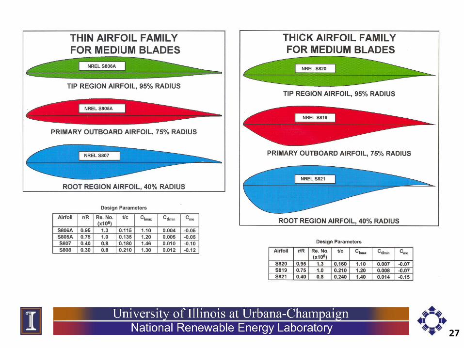
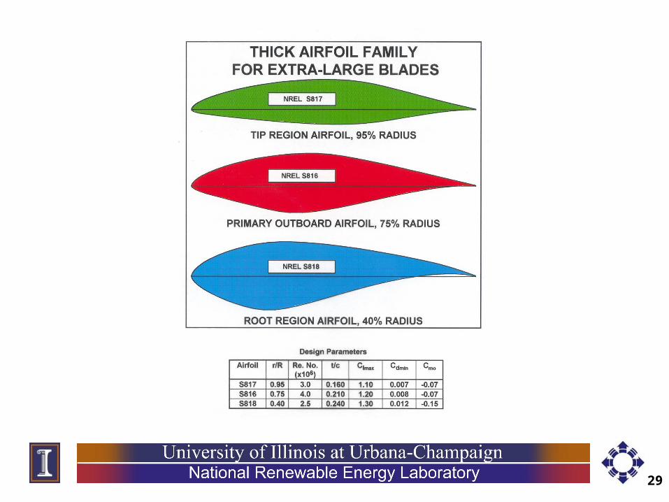
• NREL Advanced Airfoil Families
Blade Length Generator Size Thickness Airfoil Family
(meters) (kW) Category (root--------------------------------tip)
1-5 2-20 thick S823 S822
5-10 20-150 thin S804 S801 S803
5-10 20-150 thin S808 S807 S805A S806A
5-10 20-150 thick S821 S819 S820
10-15 150-400 thick S815 S814 S809 S810
10-15 150-400 thick S815 S814 S812 S813
15-25 400-1000 thick S818 S816 S817
15-25 400-1000 thick S818 S825 S826
Note: Shaded airfoils have been wind tunnel tested.

26
27

28
29

30
– Potential Energy Improvements• NREL airfoils vs airfoils designed for aircraft (NACA)

31
• Other Wind Turbine Airfoils– University of Illinois
• SG6040/41/42/43 and SG6050/51 airfoil families for small wind turbines (1-10 kW)• Numerous low Reynolds number airfoils applicable to small wind turbines
– Delft (Netherlands)– FFA (Sweden)– Risø (Denmark)

32
• Airfoil Selection– Appropriate design Reynolds number– Airfoil thickness according to the amount of centrifugal stiffening and desired blade rigidity– Roughness insensitivity most important for stall regulated wind turbines– Low drag not as important for small wind turbines because of passive over speed control and smaller relative influence of drag on performance– High-lift root airfoil to minimize inboard solidity and enhanced starting torque

33
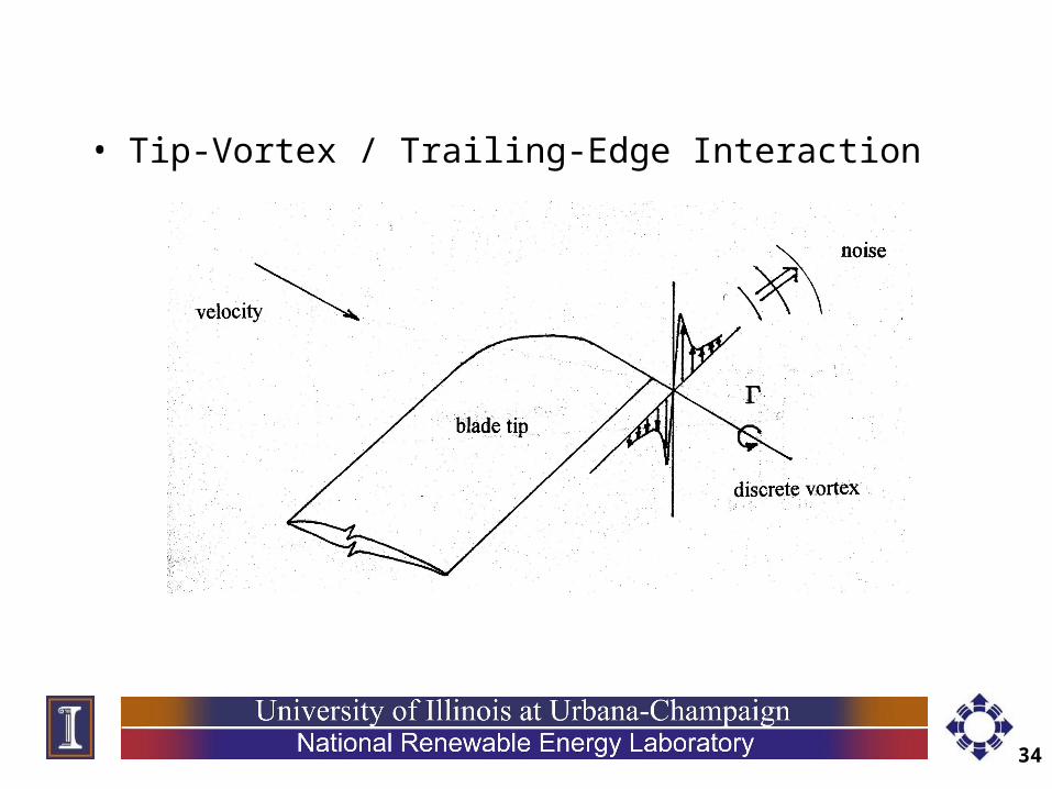
Noise Sources and Tip Shapes• Noise Sources
– Tip-Vortex / Trailing-Edge Interaction– Blade/Vortex Interaction– Laminar Separation Bubble Noise
34
• Tip-Vortex / Trailing-Edge Interaction

35
• Tip Shapes
Sword Shape Swept Tip

36
• Effect of Trailing-Edge Thickness at the Tip of the Blade

37
• Thick and Thin Trailing Edge Noise Measurements
Thick Tip trailing Edge Thin Tip Trailing Edge

38
Stall-Delay and Post-Stall Models• Stall-Delay Models
– Viterna– Corrigan & Schillings– UIUC model
39
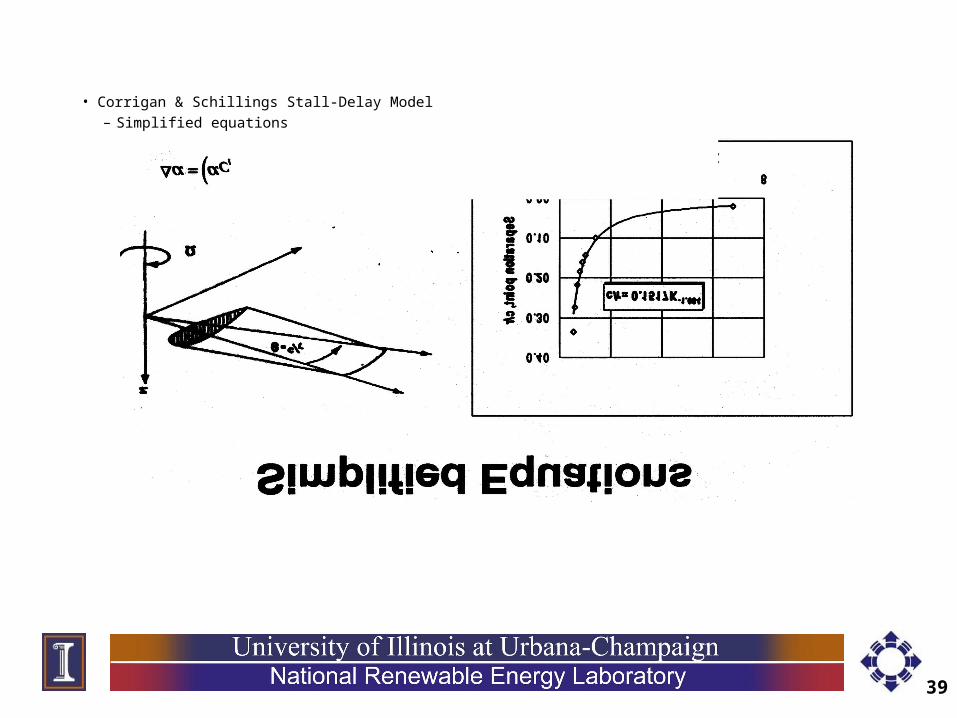
• Corrigan & Schillings Stall-Delay Model– Simplified equations

40
– CER blade geometry
41
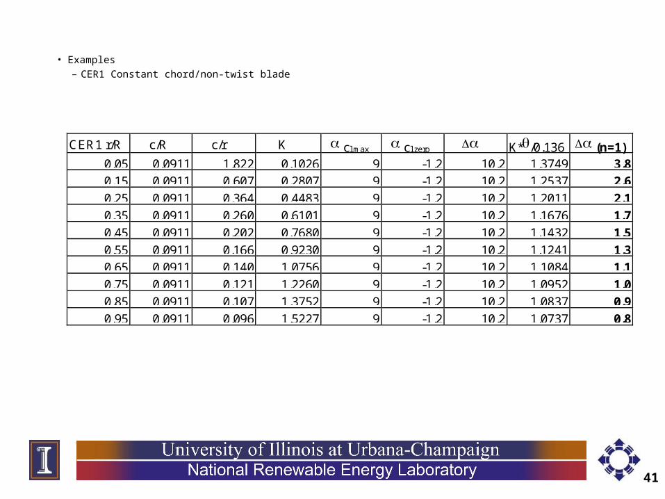
CER1 r/R c/R c/r K cl max cl zero K*/0.136 (n=1)0.05 0.0911 1.822 0.1026 9 -1.2 10.2 1.3749 3.80.15 0.0911 0.607 0.2807 9 -1.2 10.2 1.2537 2.60.25 0.0911 0.364 0.4483 9 -1.2 10.2 1.2011 2.1
0.35 0.0911 0.260 0.6101 9 -1.2 10.2 1.1676 1.70.45 0.0911 0.202 0.7680 9 -1.2 10.2 1.1432 1.5
0.55 0.0911 0.166 0.9230 9 -1.2 10.2 1.1241 1.30.65 0.0911 0.140 1.0756 9 -1.2 10.2 1.1084 1.1
0.75 0.0911 0.121 1.2260 9 -1.2 10.2 1.0952 1.00.85 0.0911 0.107 1.3752 9 -1.2 10.2 1.0837 0.90.95 0.0911 0.096 1.5227 9 -1.2 10.2 1.0737 0.8
• Examples– CER1 Constant chord/non-twist blade

42
CER3 r/R c/R c/r K cl max cl zero K*/0.136 (n=1)0.05 0.0442 0.886 0.1987 9 -1.2 10.2 1.2941 3.00.15 0.0510 0.341 0.4769 9 -1.2 10.2 1.1943 2.00.25 0.1465 0.586 0.2902 9 -1.2 10.2 1.2499 2.5
0.35 0.1364 0.390 0.4216 9 -1.2 10.2 1.2078 2.10.45 0.1263 0.281 0.5695 9 -1.2 10.2 1.1750 1.8
0.55 0.1162 0.211 0.7388 9 -1.2 10.2 1.1473 1.50.65 0.1061 0.163 0.9357 9 -1.2 10.2 1.1227 1.3
0.75 0.0960 0.128 1.1692 9 -1.2 10.2 1.1000 1.00.85 0.0859 0.101 1.4519 9 -1.2 10.2 1.0784 0.80.95 0.0758 0.080 1.8029 9 -1.2 10.2 1.0572 0.6
– CER3 tapered/twisted blade

43
0.0
0.2
0.4
0.6
0.8
1.0
1.2
1.4
-3 0 3 6 9 12 15 18
Angle of Attack, degrees
Lift
Coef
ficie
nt
0
0.2
0.4
0.6
Drag
Coe
ffici
ent
r/R=0.35
r/R=0.35
0.0
0.2
0.4
0.6
0.8
1.0
1.2
1.4
-3 0 3 6 9 12 15 18
Angle of Attack, degrees
Lift
Coef
ficie
nt
0
0.2
0.4
0.6
Drag
Coe
ffici
ent
r/R=0.35
r/R=0.35
– S809 Deflt 2-D data without/with stall delay

44
0.0
0.2
0.4
0.6
0.8
1.0
1.2
1.4
-3 0 3 6 9 12 15 18
Angle of Attack, degrees
Lift
Coe
ffici
ent
0
0.2
0.4
0.6
Drag
Coe
ffici
ent
r/R=0.35
r/R=0.55
r/R=0.75
r/R=0.95
r/R=0.35
r/R=0.55
r/R=0.75
r/R=0.95
0.0
0.2
0.4
0.6
0.8
1.0
1.2
1.4
-3 0 3 6 9 12 15 18
Angle of Attack, degrees
Lift
Coef
ficie
nt
0
0.2
0.4
0.6
Drag
Coe
ffici
ent
r/R=0.35
r/R=0.55
r/R=0.75
r/R=0.95
r/R=0.35
r/R=0.55
r/R=0.75
r/R=0.95
– CER1 airfoil data without/with stall delay

45
0.0
0.2
0.4
0.6
0.8
1.0
1.2
1.4
-3 0 3 6 9 12 15 18
Angle of Attack, degrees
Lift
Coef
ficien
t
0
0.2
0.4
0.6
Drag
Coe
fficie
nt
r/R=0.35
r/R=0.55
r/R=0.75
r/R=0.95
r/R=0.35
r/R=0.55
r/R=0.75
r/R=0.95
0.0
0.2
0.4
0.6
0.8
1.0
1.2
1.4
-3 0 3 6 9 12 15 18
Angle of Attack, degrees
Lift
Coef
ficie
nt
0
0.2
0.4
0.6
Drag
Coe
ffici
ent
r/R=0.35
r/R=0.55
r/R=0.75
r/R=0.95
r/R=0.35
r/R=0.55
r/R=0.75
r/R=0.95
– CER3 airfoil data without/with stall delay
46
02468
101214161820
0 5 10 15 20Wind Speed (m/s)
Rotor
Powe
r (kW)
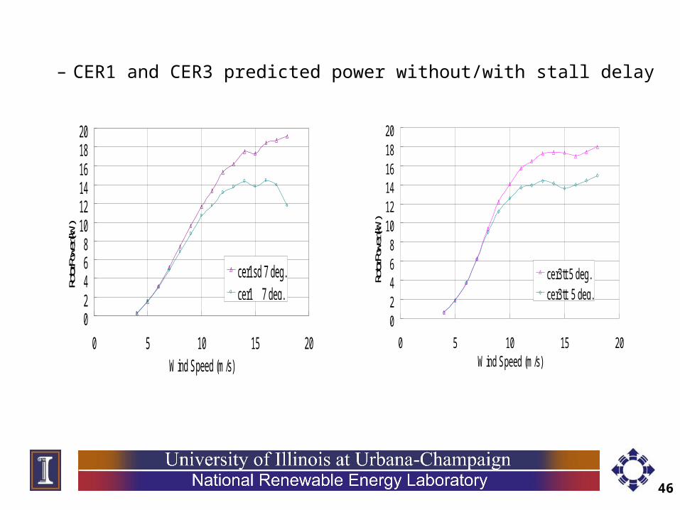
cer1sd 7 deg.cer1 7 deg.
02468
101214161820
0 5 10 15 20Wind Speed (m/s)
Rotor
Powe
r (kW)
cer3tt 5 deg.cer3tt 5 deg.
– CER1 and CER3 predicted power without/with stall delay

47
• UIUC Stall-Delay Model– Easier to tailor to CER test data than Corrigan & Schillings model– More rigorous analytical approach– Results in greater blade root lift coefficient enhancement than Corrigan & Schillings model

48
• Conclusions on Post-Stall Models– The Corrigan & Schillings stall delay model
quantifies stall delay in terms of blade geometry– Greater blade solidity and airfoil camber resulted
in greater stall delay– Tapered blade planform provided the same %
peak power increase as constant-chord blade with lower blade loads
– Predicted CER peak power with stall delay was 20% higher
– Peak power increases of 10% to 15% are more realistic for lower solidity commercial machines
Top Related