


Languages
Pages
Legal


1
Formation et Analyse d’ImagesSession 5
Daniela Hall
4 November 2004

2
Course Overview
• Session 1: – Homogenous coordinates and tensor notation– Image transformations– Camera models
• Session 2:– Camera models– Reflection models– Color spaces
• Session 3:– Review color spaces– Pixel based image analysis
• Session 4:– Gaussian filter operators– Scale Space

3
Course overview
• Session 5:– Contrast description– Hough transform
• Session 6:– Kalman filter– Tracking of regions, pixels, and lines
• Session 7:– Stereo vision – Epipolar geometry
• Session 8: exam

4
Session overview
1. Contrast description
2. Hough transform

5
Feature extraction in computer vision
• The goal of feature extraction is – Reduce the amount of information– Simplify the interpretation– Preserve the information necessary for further
processing (task dependent)
• The ideal feature extraction alogrithm is invariant– Invariance: the observation is the same independent of
the view point and illumination.
• Contours are good candidates for invariant feature extraction

6
Contrast
• Contrast can be caused by– Change in surface orientation (discontinuity in depth)
• useful for description of polyhedrical objects
– Limit of a shadow• useful to recognize 3D object form
– Texture on a surface• independent of surface, can be used to recover the texture
– Reflections• depends on view point and illumination

7
Contrast detection process
Image processing
Image analysisimage
intermediateimage representation
image description

8
Contrast detection methods
• Search for extremum in 1st derivative
• Search for zero crossing in 2nd derivative

9
Contrast detection
Step edge Smoothedstep edge
First derivative Second derivative(white pos, yellow negative)

10
Image processing tools
• Let s(i), f(i) be two real discrete signals
• s(i) has Ns discrete values on the interval 0<=i<=Smax
• f(i) has Nf discrete values on the interval 0<=i<=Fmax
• Pmax=min{Smax,Fmax}
• s(i)=0 for all i<0, Smax<i
• f(i)=0 for all i<0, Fmax<i
• The scalar product of s(i) and f(i) is a scalar p
1max
0
)()()()()(),(P
ii
ifisifisifisp

11
Correlation and convolution
• Correlation is a scalar product with an offset k over all values of k.
• Convolution is a correlation where one of the signals is flipped (i-k)->(Fmax-1)-(i-k)
1max1max
0
)()()()()()(
)(),()()()(kF
ki
S
ii
kifisifkisifkis
ifkisifiskc
kF
ki
S
i
kiFfisiFfkis
iFfkisifiskr1max
max
1max
0max
max
))()1(()()1()(
))1((),()()()(

12
Contrast detection
• Roberst contrast detector
• Sobel contrast detector
• Difference filters

13
Roberts contrast detector
• Consists of two masks m1(i,j)= and m2(i,j)=1 0
0 -1
0 1-1 0
4)
),(
),((tan),(
),(),(),(
),(),(),(
1
21
22
21
1
0
1
0
jiE
jiEji
jiEjiEjiE
LkmLjkipmpjiEk L
nnnCompute correlation
for n=1,2:Contrast magnitude
Contrast direction

14
Roberst contrast detector
• The detector is very sensitive to high frequency noise.
• This sensitivity can be reduced by a low pass filtering.

15
Sobel detector
• very popular detector (Duda-Hart 1972)
m0(i,j)= m90(i,j)=
• This filter can be seen as a convolution of two components:
m0(i,j)= * m90(i,j)= *
1 0 -12 0 -21 0 -1
1 2 10 0 0-1 -2 -1
121
-1 0 1-101
1 2 1

16
Sobel detector
• As for Roberst the amplitude and orientation are computed by:
4)
),(
),((tan),(
),(),(),(
),(),(),(
0
901
290
20
1
0
1
0
jiE
jiEji
jiEjiEjiE
LkmLjkipmpjiEk L
nnnCompute correlation
for n=1,2:Contrast magnitude
Contrast direction

17
Examples
Original image Roberts detector
Sobel detector Smoothing bybinomial filters7
Differencefilter -1 0 1
Difference filter -1 1

18
Contrast detection by derivatives
• Steps:– Smoothing: suppression of noise– Computation of gradient magnitude and orientation– Local extremum detection by hysteresis thresholding– Edge segment extraction

19
Smoothing by binomial filters
• Binomial filters are the best approximation of a discrete Gaussian with integer values.
• Binomial filters are generated by n convolutions of [1 1]
• Binomial series: The binomial series is composed of the coefficients of the polynom
!)!(
!
)(
,
2/
2/,
mmn
n
m
nb
yxbyx
nm
n
nm
mmnnm
n

20
The binomial series• The coefficients of the binomial series can
be generated by Pascal’s triangle
1 1 1
1 2 1 1 3 3 1 1 4 6 4 1 1 5 10 10 5 1 1 6 15 20 15 6 1 1 7 21 35 35 21 7 11 8 29 56 70 56 29 8 1
Level(n)012345678
Sum1248163264128256
Variance0¼½¾15/46/47/42

21
Binomial filters
• n convolutions of [1 1]
• Gain: 2n
• Variance: var{bn(m)}=n var{b1(m)} = n/4
• discrete Gaussian with sigma = 1: 1 4 6 4 1
• sigma= 2: 1 8 29 56 70 56 29 8 1
• sigma=0.5: 1 2 1

22
Discrete Gaussian filter
• discrete Gaussian with sigma = 1: 1 4 6 4 1
• Gain: 24=16
G(x,1.0) |0.004|0.054|0.242|0.399|0.242|0.054|0.004|
Example of sampling a 1D Gaussian (sigma=1, R=3) session 4
16 G(x,1.0) |0.064|0.864|3.872|6.384|3.872|0.864|0.064|

23
Contrast detection by derivatives
• Steps:– Smoothing: suppression of noise– Computation of gradient magnitude and orientation– Local extremum detection by hysteresis thresholding– Edge segment extraction
24
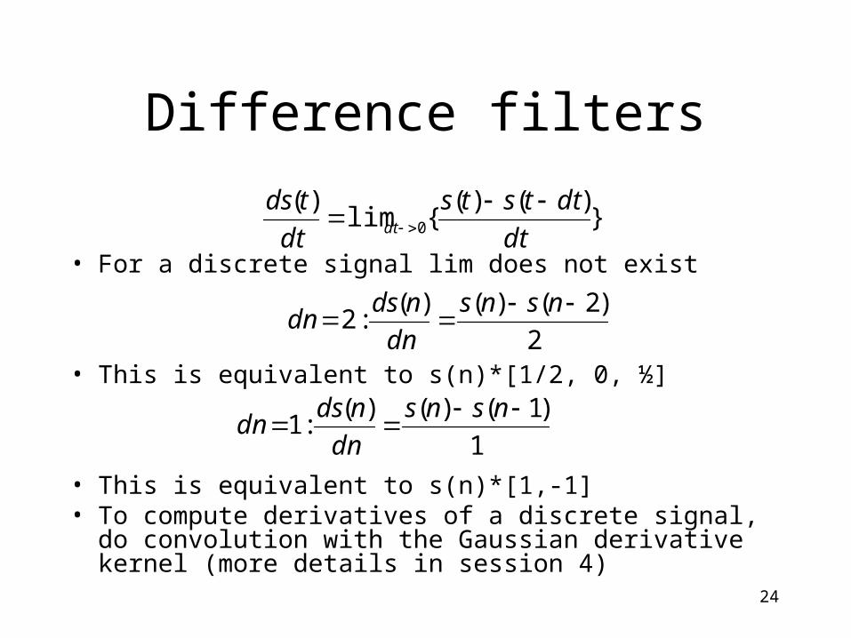
Difference filters
• For a discrete signal lim does not exist
• This is equivalent to s(n)*[1/2, 0, ½]
• This is equivalent to s(n)*[1,-1]• To compute derivatives of a discrete signal, do
convolution with the Gaussian derivative kernel (more details in session 4)
})()(
{lim)(
0 dt
dttsts
dt
tdsdt
2
)2()()(:2
nsns
dn
ndsdn
1
)1()()(:1
nsns
dn
ndsdn

25
Difference filters
• Alternative method to convolution with Gaussian derivative kernel are the difference filters.
• Smoothing followed by a difference filter is equivalent to the Sobel operator.
-1 0 1 -1 0 1

26
Examples
Original image Roberts detector
Sobel detector Smoothing bybinomial filters
Differencefilter -1 0 1
Difference filter -1 1

27
Examples
Original image Roberts detector
Sobel detector Smoothing bybinomial filters7
Differencefilter -1 0 1
Difference filter -1 1

28
Contrast detection by derivatives
• Steps:– Smoothing: suppression of noise– Computation of gradient magnitude E(i,j) and direction theta– Local extremum detection and hysteresis thresholding– Edge segment extraction

29
Local extremum detection
• Find direction of maximum gradient. Without loss of generality, let the direction be (1, 0)T
• Check if E(i,j) is a maximum in this direction• This means:
– Find contrast points C(i,j) that fulfill
else0
),(),(),(
and 0),(1
),( jjiiEjiEjjiiE
jiEjiC

30
Hysteresis thresholding
• Problem: some detectors produce weak edges which should be eliminated.
• Solution: hysteresis thresholding• Properties: eliminates weak edges below a low
threshold, but not if they are connected to an edge above a high threshold.
weak edge
strongedge
C(i,j) C(i,j) afterchaining

31
Hysteresis thresholding
• Uses a high and a low threshold– low threshold th0: sensitive to noise, but
produces contour candidates– high threshold th1: indicates strong edges
1. Compute map F(i,j) with two thresholds th0, th1
else0
th1j)E(i, th0if1
|j)E(i,| th1if2
),( jiF

32
Hysteresis filtering
2. Computing connected components of edge elements
An edge is selected when it contains at least one strong edge element (with label 2).
Edges consisting of only weak edge elements are discarded.

33
Hysteresis filtering
• The thresholding and chaining can be computed in one step.
• Start with the high threshold image.
• For each strong edge continue adding (8 or 4) connected pixels with E(i,j)>=th0.

34
Example
original image Contourimage
Low threshold image
High thresholdimage

35
Contrast detection methods
• Search for extremum in 1st derivative: ok
• Search for zero crossing in 2nd derivative

36
Contrast detection by 2nd derivatives
• The Laplacien is a isotropic filter that is used for the contrast detection.– Lap(i,j)= Lxx(i,j) + Lyy(i,j)– with Lxx(i,j)= I(i,j) * Gxx(sigma)
• As for Gaussians there exists a integer approximation of the Laplacian.– Lxx(i,j) : [ 1 -1] * [1 -1] = [-1 2 -1] – Lxx(i,j)+Lyy(i,j):
* + * =0 -1 0-1 4 -10 -1 0
0 0 0 0 1 00 0 0
-1 2 -1
0 0 0 0 1 00 0 0
-12-1

37
Gradient norm and Laplacian

38
Example
image Lap
Differenceimage Lx
Differenceimage Ly

39
ExampleDifference image Lx Laplacian

40
Example
image Lap
Differenceimage Lx
Differenceimage Ly

41
Contour detection by 2nd derivatives
• In theorie:– Contours can be detected more precisely using
zero-crossing of 2nd derivative. – Sub-pixel precision is possible by interpolation.– zero crossing of 2nd derivatives produce closed
contours.
• In real life:– The zero crossing of the 2nd derivative detect
also many small unstable regions.

42
Detection of zero crossing
• The extrema of the 1st derivative correspond to zero crossing of the 2nd derivative.
• To generate a contour image C(i,j) proceed as follows:– consider 4-connected neighbors (N,S,W,E)
else0
0||)()(or
0|WE|)()(1
),( NSSsignNsign
EsignWsignjiC

43
Detection of zero crossing
• For a stabler detection add a term that is related to the strength of the edge.
• Disadvantage: this measure may break a closed contour. The contours are no longer closed.
else0
thres|S- N|0||)()(or
thres|E-W |0|WE|)()(1
),( NSSsignNsign
EsignWsignjiC

44
Session overview
1. Contrast description
2. Hough transform
45
Hough transform
• The Hough transform is a standard tool in image analysis that allows recognition of global patterns in an image space by recognition of local patterns in a transformed parameter space.
• It is particularly useful when the patterns one is looking for are sparsely digitized, have ``holes'' and/or the pictures are noisy.
• The basic idea of this technique is to find curves that can be parameterized like straight lines, polynomials, circles, etc., in a suitable parameter space.
Hough59 P.V.C. Hough, Machine Analysis of Bubble Chamber Pictures, International Conference on High Energy Accelerators and Instrumentation, CERN, 1959.

46
Hough transform
• Although the transform can be used in higher dimensions the main use is in two dimensions to find, e.g. straight lines, centres of circles with a fixed radius, parabolas y = ax2 + bx + c with constant c, etc.
• As an example consider the detection of straight lines in an image. We assume them parameterized in the form: y=mx+c
• Each image point (x,y) gives rise to a certain number of possible values for m and c.
• This set of values forms a line c=-mx+y in the Hough space (m,c)• When the contour points are aligned, the corresponding lines in the
Hough space have the same intersection point (m0,c0). • A point in hough space indicates a line in the image space.
source: http://rkb.home.cern.ch/rkb/AN16pp/node122.html

47
Hough transform
• Computation:– Initialise histogram h(m,c) (this represents the Hough
space)
– for each image point (i,j)• if C(i,j)=1, then compute all possible couples (m,c) that pass
through the point (i,j).
• increment all corresponding cells by 1.
– A local maximum (m0,c0) in h(m,c) indicates that the image points are aligned to the line y=m0 x+c0

48
Hough transform
• Problems:– Care has to be taken when one quantizes the parameter
space. • When the bins table are chosen too fine, the local maximum
can be dispersed over several bins.
• When the quantization is not fine enough, on the other hand, nearly parallel lines which are close together will lie in the same bin.
– The coefficients m,c are not uniform in orientation• Solution: use a different parameterization (p,theta):
x sin(theta)-y cos(theta) + p =0

49
Hough transform
– Use a different parameterization (p,theta): x sin(theta)-y cos(theta) + p =0
– p is the distance from the origin and theta the angle with the normal
– Here each point in the image space corresponds to a sinusoidal curve in the Hough space. The intersection of the sinusoidal curves in the Hough space correspond to a line in the image space.

50
Hough transform
• Computation:– Initialise histogram h(p,theta) (this represents the
Hough space)
– for each image point (i,j)• if C(i,j)=1, then
– for all 0<theta<2pi compute p=-i sin(theta)+j cos(theta)
– set h(p,theta) = h(p,theta)+1
– A local maximum (p0,theta0) in h(p,theta) indicates that the image points are aligned to the line
p0=-x sin(theta0)+y cos(theta)

51
Generalised Hough transform
• You can compute the hough transform for any pattern that can be parameterized, such as circles, lines, parabolas.
• For circles:(x-a)2 + (y-b)2 = r2
• We use a hough space h(a,b,r).• Each image point corresponds to a cone in space (a,b,r)• For a fixed r, each image point corresponds to a circle in hough space.• Algorithm:
– for each image point and each radius r>0 compute the corresponding circle in hough space. Increment all cells.
– After filling the histogram, locate the local maximum (a0,b0,r0). This maximum corresponds to the circle in the image with center (a0, b0) and radius r0.
Top Related