NBER WORKING PAPER SERIES

INFLATION AND THE ROLE OF BONDSIN INVESTOR PORTFOLIOS

Zvi Bodie

Alex Kane

Robert McDonald

Working Paper No. 1091

NATIONAL BUREAU OF 0JONOMIC RESEARCH1050 Massachusetts Avenue

Cambridge MA 02138

March 1983

This paper was prepared as part of the National Bureau of EconomicResearch Program in Financial Markets and Monetary Economics and Projecton the Changing Roles of Debt and Equity in Financing U.S. CapitalFormation, which was financed by a grant from the American Council ofLife Insurance. It was presented at the NBER Conference on CorporateCapital Structures in the U.S., in Palm Beach, Florida, on January 6and 7, 1983. Zvi Bodie is Associate Professor of Finance at BostonUniversity School of Management and NBER Research Associate. Alex Kaneand Robert McDonald are both Assistant Professors of Finance at Boston

University School of Management. Robert McDonald is also an NBER ResearchFellow. Any opinions expressed are those of the authors and not thoseof the National Bureau of Economic Research.

NEER Working Paper #1091March 1983

Inflation and the Role of Bonds in Investor Portfolios

Abstract

This paper explores both theoretically and enirically the role ofnominal bonds of various maturities in investor portfolios in the U.S. One ofits principal goals is to determine whether an investor who is constrained tolimit his investment in bonds to a single portfolio of money—fixed debt instru-ments will suffer a serious welfare loss. Our interest in this question stemsin part from the observation that many employer—sponsored savings plans limit aparticipant's investment choices to two types, a common stock fund and a money—fixed bond fund of a particular maturity. A second goal is to study the desira-bility and feasibility of introducing a market for index bonds (i.e. an assetoffering a riskiess real rate of return) in the U.S. capital markets.

The theoretical framework is Merton's (1971) continuous time model ofconsumption and portfolio choice. Our measure of the welfare gain or loss froma given change in the investor's opportunity set is the increment to currentwealth needed to completely offset the effect of the change. A novel feature ofour empirical approach is the method of deriving equilibrium risk premia on thevarious asset classes. We employ the variance—covariance matrix of real ratesof return estimated from historical data in combination with "reasonable"assumptions about net asset supplies and the econonbr_wide average degree of riskaversion to derive numerical values for these risk premia. This procedureallows us to circumvent the formidable estimation problems associated with usinghistorical means, which are negative during some subperiods.

Our main results are: (i) There can be a substantial loss in welfarefor participants in savings plans offering a choice of only two funds, a diver-sified stock fund and an intermediate—term bond fund. !bst of this loss can beeliminated by introducing as a third option a money market fund. (2) Thepotential welfare gain from the introduction of private index bonds in the U.S.capital market is probably not large enough to justify the costs of innovation.The major reason for the swall gain is that one month bills with their smallvariance of real returns are an effective substitute for index bonds.

Zvi Bodie, Alex Kane and Robert McDonaldSchool of ManagementBoston University7014 Commonwealth AvenueBoston, MA 02215

j

—1—

Inflation and the Bole of Bonds in Investor Portfolios.

I. Introduction

The inflation of the past decade and a half has dispelled the notion

that default—free nominal bonds are a riskless investment. Conventional wisdom

used to be that the conservative investor invested principally in bonds, and the

aggressive or speculative investor invested principally in stocks. Short—term

bills were considered to be only a temporary "parking place" for funds awaitinginvestment in either bonds or stocks. Thdv many academics and practitioners in

the field of finance have come to the view that for an investor who is concerned

about his real rate of return, long—term nominal bonds are a risky investment

even when held to maturity.

The alternative view that a policy of rolling—over short term bills

might be a sound long—term investment strate' for the conservative Investor has

recently gained credibility. The rationale behind this view is the observation

that for the past few decades, bills have yielded the least variable real rate

of return of all the major investment instruments traded in U.S. financial

markets. Stated a bit differently, the nominal rate of return on bills hastended to mirror changes in the rate of inflation so that their real rate bfreturn has remained relatively stable as compared to stocks or longer term

fixed—interest bonds.

This is, of course, not a coincidence. All market—determined interest

rates contain an "inflation premium," which reflects expectations about the

declining purchasing power of the money borrowed over the life of the loan. Asthe rate of inflation has increased in recent years, so too has the Inflation

premium built into interest rates. While long—terni as well as short—term

_0

interest rates contain such a premium, conventionallong—term bonds lock the

investor into the current interest rate for the life of the bond. If long—terminterest rates on new bonds subsequently rise as a result of unexpected infla-

tion, the funds already locked in can be released only by selling the bonds on

the secondary market at a price well below their face value. But if an investor

buys only short—term bonds with an average maturity of about thirty days, then

the interest rate he earns will la€ behind changes in the inflation rate by at

most one month. For the investor who is concerned about his real rate of

return, bills may therefore be less risky than bonds, even in the long run.

The main purpose of this paper is to explore both theoretically and

empirically the role of nominal bonds of various maturities ininvestor port-

folios. i-low important is it for the investor to diversify his bond holdings

fully across the range of bond maturities? We provide a way to measure the

importance of diversification, and this enables us to determine the value of

holding stocks and a variety of bonds, for example, as opposed to following aless cumbersome investment strater, such as concentrating in stocks and bills

alone.

One of our principal goals is to determine whether an investor who is

constrained to limit his investment in bonds to a single portfolio of money—

fixed debt instruments will suffer a serious welfare loss. In part, our

interest in this question stems from the observation that many employer—

sponsored tax—deferred savings plans limit a participantts investment choices to

two types, a common stock fund and a money—fixed bond fund of a particular

maturity?

—3—

A second goal is to study the desirability of introducing a market for

indexed bonds (i.e. an asset offering a riskiess real rate of return). There

is a substantial literature on this subject,2 but to our knowledge no one has

attempted to measure the magnitude of the welfare gain to an individual investor

from the introduction of trading in such securities in the U.S. capital market.

In the first part of the paper we develop a mean—variance model for

measuring the value to an investor of a particular set of investment instruments

as a function of his degree of risk aversion, rate of time preference and

investment time horizon. We then take ianthly data on real rates of return on

stocks, bills and U.S. government bonds of eight different durations, their

covariance structure, and combine these estimates with reasonable assumptions

about net asset supplies and aggregate risk aversion in order to derive a set of

equilibrium risk premia. This procedure allows us to circumvent the formidable

problems of deriving reliable estimates of these risk premia from the historical

means, which are negative during many subperiods. We then employ these para-

meter values in our ndel of optimal consumption and portfolio selection in

order to address the two empirical issues of principal concern to us. The paper

concludes with a section summarizing the main results and pointing out possible

implications for private and public policy.

II. Theoretical Jbdel

A. tdel Structure and Assumptions

Our basic model of portfolio selection is that of Markowitz (1952) as

extended by Merton (1969 and 1911). Merton has shown that when asset prices

follow a Geometric Browr-xian Motion in continuous time and portfolios can be con—

tinuously revised, then as in the original Markowitz model, only the means,

variances and covariances of the joint distribution of returns need to be con-

sidered in the portfolio selection process.

In more formal terms we assume that the real return dynamics on all n

assets are described by stochastic differential equations of the form:

dQ= R.dt + a.dz

Q. i i

2where R. is the mean real rate of return per unit time on asset i and thevariance per unit time. For notational convenience we will let R represent the

n—vector of means and 1 the nxn covariance matrix, whose diagonal elements are

the variances and whose off—diagonal elements are the cowariances

Investors are assumed to have homogeneous expectations about the values

of these parameters. Furthermore, we assume that all n assets are continuouslyand costlessJ,y traded and that there are no taxes.3

The change in the individual's real wealth in any instant is given by:

11 n(i) dW = WSw•R•dt — Cdt + WEw,a•dz111 111 1where W is real wealth, C is the rate of consumption, and w• is the proportionof his real wealth invested in asset i.

—5—

The individual's optirial consumption and portfolio rules are derived by

finding:

—p(2) 1uax1 E0J e U(C)dtn,,Wj U

where E is the expectation operator, p is the rate of time preference, u(c)

the utility from consumption at time t, and H is the end of the investor's

planning horizon.

The individual's derived utility of wealth function is defined as;

(3) J(W) = maxEt

J is interpreted as the discounted expected value of lifetime utility,

tonditional upon the investor's following the rules for optimal consumption and

portfolio behavior. This value can be computed as a function of current wealth.

The specific utility function with which we have chosen to work is the well—

known constant relative risk aversion form:

I

u(c) = for y C 1 and I 0

logC fory=0

with 6 E 1 — y representing Pratt's measure of relative risk aversion. This

functional form has several desirable properties for our purposes. First, the

investor' s degree of relative risk aversion is independent of his wealth, which

in turn inlies that the optinal portfolio proportions are also independent of

wealth. Secondly, actually solving the problem in (2) allows us to find an

explicit solution for the derived utility of wealth function (Merton 1971),

which takes the relatively simple form:

—6—

WY(1) (w) =I

p — '(V1—ewhereq=

Is

and v is a number which reflects the parameters of the investor's investment

opportunity set and his degree of risk aversioni Specifically, when there isno risk—free asset, v is defined by:

A D 6() v =—+—————G 2G6 2G

where

A

—1B E R'4 B

ci

D - A2

where i is a vector of dimension n all of whose elements are 1.

The degree of relative risk aversion plays an important role in the

specific numerical results which follow, so we interpret this parameter by means

of a simple example. Suppose an individual faces a situation in which there is

a .5 probability of losing a proportion x of his current wealth and a .5 proba-

bility of gaining the same proportion. What proportion of current wealth would

the individual be willing to pay a an insurance premium in order to eliminate

this risk?5

Table 1 displays the value of this insurance premium for various values

of x and 6. The second row, for example, shows that for a risk which involves a

gain or loss of 10% of current wealth an investor with a coefficient of relative

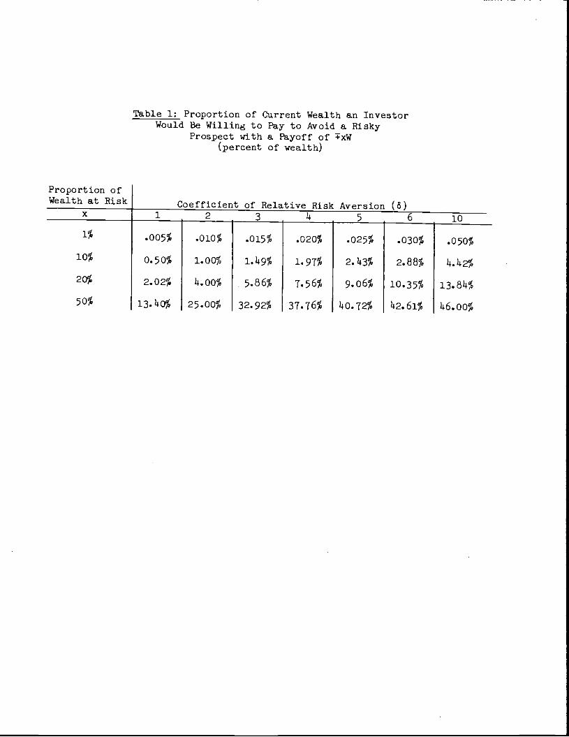
Table 1: Proportion of Current Wealth an InvestorWould Be Willing to Pay to Avoid a Risky

Prospect with a Payoff of xW(percent of wealth)

Proportion ofWealth at Risk Coefficient of Relative Risk Aversion (5)

x 1 2 3 ________ 5 6 10

.oo% .010% .015% .020% .025% .030% .050%

10% 0.50% i.oo% 1.49% 1.91% 2.43% 2.88% 4.42%

20% 2.02% 5.86% 1.56% 9.06% 10.35% 13.84%

50% 13.40% 25.00% 32.92% 37.76% 40.72% 42.61% 46.oo%

—7—

risk aversion of 1 would only pay one half of one per cent of his wealth (or 5%of the magnitude of' the possible loss) to insure against it, while an investorwith a 6 of 10 would pay b.142% of his wealth (which is fully 14b.2% of the nugni—

tude of the possible loss). If the investor with a 6 of 10 faces a riskyprospect involving a possible gain or loss of 50% of his wealth, he would be

willing to pay 92% of the possible loss to avoid the risk.

B. Optimal Portfolio Proportions and Equilibrium Risk Premia

The vector of optimal portfolio weights derived from the optimizationmodel described above is given by;

(6) w* l1(R —- j) +

Note that these weights are independent of the investor's rate of tine pre-

ference and his investment horizon. Merton (1912) has shown that4-

is the mean—l

rate of return on the minimum variance portfolio and that is the vector of

portfolio weights of the n assets in the minimum variance portfolio. Denoting

these by Ri and WI, respectively, we can rewrite equation (6) as:

* 1 —l(6') w U (R — B i) + w

6 nan nan

The demand for any individual asset can thus be decomposed into two

parts represented by the two terms on the right hand side of equation (7):

—8—

* in(y) v(ri —R•' ói=i ii .1 nan i,min

where v•, is the th element of the inverse of the covariance matrix. Thefirst of these two parts is a "speculative demand" for asset i, which depends

inversely on the investor's degree of risk aversion and directly on a weightedsum of the risk prenia on the n assets. The second coxnponent is a "hedgingdemand" for asset i which is that asset's weight in the minilmlm_variance

portfolio. 6

Under our assuniption of homogeneous expectations the equilibriwn riskpreinia on the n assets are found by aggregating the individual demands for eachasset (equation 6') and setting them equal to the supplies. The resultingequilibrium yield relationships can be expressed in vector form as:

— 2(8) B — B i = — a 1)nan M nan

where 6 is a harmonic nan of the individual investors' asures of risk aver-

sion weighted by their shares of total wealth, is the vector of net supplies

of the n assets each expressed as a proportion of the total value of all assets,

and a2 is the variance of the miniraim variance portfolio.

The portfolio whose weights are given by has co to be known in the

literature on asset pricing as the "market" portfolio, and we will adopt that

same terminolor here. Equation (8) implies that:

—9—

— 2(9) B. — B . = a. — a1 nan iM mm

where a is the covariance between the real rate of return on asset i and therate of return on the market portfolio.

This relationship holds for any individual asset and for any portfolio

of assets. Thus for the market portfolio we get:

(10) R — B = Z(2 — 2M man M nan

It is interesting to compare this with the traditional form of the Capital Asset

Pricing Model which assumes the existence of a riskless asset. In that special2case B. sLIiy the riskless rate and a mm is zero.

By substituting the equilibrium values of B. — R from equation (8)

into equation (61), we get for investor k;

6(11) w —vk M manK k

This implies that in equilibrium every investor will hold some combination of

the market and the minimum variance portfolios. If the investor is rmz're risk

averse than the average he will divide his portfolio into positive positions in

both the market portfolio and the mininum variance portfolio, with a higher

proportion in the latter the greater his degree of risk aversion. If he is

less risk averse than the average he will sell the mininum variance portfolio

short in order to invest more than 100 percent of his funds in the market port-

folio.

—1°-

c. The Welfare Loss from Incomplete Diversification

Suppose the invesbor faces an investment opportunity set consisti of

less than the full set of n assets. How much additionalcurrent wealth would he

have to be given in order to make him as well off as he was with the fall set of

n assets?

Let n) be the lifetime utility of an investor who chooses from

among n assets, and let (w n — in) be the lifetime utility of an investor

choosing from among a restricted set of assets. Let W represent the investor's

actual Level of current wealth and W the level at which his welfare would be the

same under the restricted opportunity set. W is defined by:

n) = J(w j n - m)

Thus W — W is the extra wealth necessary to compensate the investor for

having a restricted opportunity set and is greater than or equal to zero. From

equation (4) we get:

—_YV)6

(12) Q=w[ i±-e 6 (p—yv)yr

(p — iv) — IV\{l—e 6

where v is calculated according to equation (5) and corresponds to the

restricted opportunity set.1

Equation (12) implies that the magnitude of the welfare loss will in

general depend on the investorts risk aversion, 6, rate of time preference, P,

and investment horizon, H. Since W is proportional to 4! a convenient measure of

this loss, which is independent of the investor's wealth level, is 1.. 1, the

loss per dollar of current wealth. Since W>W, this number is always greater

than or equal to zero.

—11—

Of course, certain restrictions on the investment opportunity set need

not decrease investor welfare. We know from equation (ii) that even if the

investor had only two mutual funds to choose from, there would be no loss in

welfare, provided they were the market portfolio and the rainimunt variance port-

folio. trton (1972) has shown that any two portfolios along the mean—variance

portfolio frontier would serve as well. But, in general, restricting the number

of assets in the opportunity set does lead to a loss in investor welfare.

D. The Shadow RLskless Hate and the Gain from Introducing a Riskiess Asset

We define the shadow riskless real rate of interest as that rate atwhich an investor would have no change in welfare if his opportunity set were

expanded to include a riskless asset. When the investment opportunity set

includes a riskiess asset, Merton (1971) shows that the lifetime utility ofwealth function is the same as (14), except that V is replaced by A, where:

—1(R —R1i)' (B—ni)

(13)26

We find the expression for the shadow riskless rate by setting U equal

to A, and solving for This gives:

(11e) = B — 'Sc2F mtn mm

This implies that a risk averse investor will always have a shadow riskiess real

rate which is less than the mean real return on the minimum variance portfolio.

The return differential is equal to his degree of relative risk aversion times

the variance of the minintun variance portfolio.

—12—

If there is a zero net supply of this riskless asset in the econontr,

the equilibrium value of will just be B. — ci21. Therefore, by assump-tion, an investor with average risk aversion will not gain from the introductionof a market for index bonds. For an investor whose risk aversion is different

from the average there will be a welfare gain, ignoring the costs of

establishing and operating such a market. We measure this gain analogously to

the way we measured the welfare cost of incomplete diversification in the pre-

vious section.

As before, let W be the investor's actual level of wealth and W the

level at which his welfare would be the same under an opportunity set expanded

to include a riskless asset offering a real rate of — Since in

this case W<W, we take as our measure of the welfare gain from indexationTn

1 — or the amount the investor would be willing to give up per dollar of

current wealth for the opportunity to trade index bonds.

—13—

III. The Data and }rameter Estimates

In this section we will describe our data and how we used them to esti-

mate the parameters needed in evaluating the welfare loss from restricting an

investor's opportunity set and the gain from introducing a real riskless asset.

It must be borne in mind that we were not trying to empirically test the model

of capital market equilibrium presented in section II but rather to derive its

implications for the specific questions being addressed in this paper. It was

therefore important to maintain consistency between the underlying theoretical

model and the parameter estimates derived from the historical data, even if that

meant ignoring some of the descriptive statistics yielded by those data.

Our raw data were monthly real rates of return on stocks, one—month

U.S. Government Treasury Bills, and eight different U.S. bond portfolios. We

used monthly data in order to best approximate the continuous trading assumption

of Merton's model, and because one month is the shortest interval for which

information about the rate of inflation is available. The measure of the price

level that we used in computing real rates of return was the Bureau of labor

Statistics' Consumer Price Index, excluding the cost—of—shelter component. We

excluded the cost of shelter component because it gives rise to well—known

distortions in the measured rate of inflation.

The bill data are from Ibbotson and Sinquefield (1982), while the bond

data are from the U.S. Government Bond File of the Center for Research in

Security Prices (CRSP) at the University of' Chicago. The stock data are from

the CRSP monthly NYSE file. We divided the bonds into eight different port-

folios based on duration. We felt that duration was superior to maturity as a

—1

criterion for grouping the bonds since it takes into account a bond's coupon as

well as its maturity.8 The durations of the bond portfolios range from one to

eight years.Table 2 presents the means, variances and correlation coefficients of

the monthly real rates of return on the ten asset categories for three sub—

periods between January 1953 and December 1981. The first is the twelve years

from January 1953 to December 19614, a period of relative price stability; the

second is the eight years from 1965 to 1972, a period of moderate inflation; and

the third is the nine years from 1973 to 1981, a period of relatively rapid

inflation.

The measure of the real rate of return used in all cases was the

natural logarithm of the monthly real wealth relatives Q.(t)/Qjt — i). On the

assumption that these returns follow a geometric Brownian motion in continuous

tline:

dQ. = R.dt + a.dz.

the log of the wealth relative over a discrete time interval is normally distri-

buted with mean and variance a2 where

2a.

= R. —4

The means reported in 'lb1e 2 were converted to annual rates by multiplying

them by 12 and the standard deviations by multiplying them by /T. This

makes them comparable to the means and standard deviations one would obtain

using a one year holding period.

Table 2: Distribution of Monthly Real Rates of Return

(annualized)

A. 1953-.19614Common lmonth Bonds (by duration in years)Stocks Bills 1 2 3 14 5 6 7 8

Mean .1202 .0113 .0183 .0213 .0218 .0151 .0188 .0122 .007)4 .02143

StandardDeviation .1179 .0081 .0105 .0170 .0235 .0268 .0311 .0305 .0361 .0155

Number ofObservations 11414 11414 11414 11*14 11414 114)4 138 110 81* 12

CorrelationCoefficients:

Stocks .014 —.02 —.09 —.10 —.06 —.13 —.15 —.12 .15Bills .70 .140 .25 .23 .22 .214 .25 .142

Bonds 1 .81 .70 .68 .65 .65 .56 .632 .85 .82 .78 .80 .'r14 .593 .90 .83 .82 .80 .604 .86 .86 .83 .65

5 .88 .86 .796 .91 .757 .95

B. 1965—1972Common lmonth Bonds (by duration in years)Stocks Bills 1 2 3 1* 5 6 7 8

Mean .01413 .0122 .0162 .0179 .0101 .0007 .0032 .0078 .0339 .0113

StandardDeviation .13145 .00614 .0155 .0298 .0370 .01427 .0519 .01427 .0453 .0377

Number ofObservations 96 96 96 96 96 96 96 52 30 6

CorrelationCoefficients:

Stocks .11 .25 .33 .38 .33 .33 .08 .03 .23

Bills .614 .52 .37 .38 .27 .32 .38 0

Bonds 1 .86 .78 .74 .67 .69 .6o .11

2 .83 .80 .73 .76 .77 .98

3 .82 .814 .85 .86 .57

Ii .83 .86 .149 .1*1

5 .914 .77 .6i

6 .66 .72

7 .88

C. 1973—1981Comnon lmonth Bonds (by duration in years)Stocks Bills 1 2 3 14 5 6 y 8

Mean —.0269 —.0050 _.001t4 —.0141 —.0186 —.0284 —.0320 —.0549 —.0298 —.01485

StandardDeviation .1735 .0126 .0316 .0529 .0693 .0812 .0922 .1034 .1049 .1095

Number ofObserve.— 108 108 108 108 108 108 108 95 99 106tioris

CorrelationCoefficients:

Stocks .20 .32 .32 .27 .31 .22 .22 .30 .33Bills .514 .39 .35 .35 .26 .22 .2f .22Bonds 1 .88 .85 .82 .80 .73 .78 .77

2 .94 .92 .87 .81 .85 .863 .95 .93 .85 .88 .88

.91 .83 .89 .875 .89 .92 .896

.91 .887

.91

Notes: The measure of the real rate of return used is thenatural logarithm of the monthly real wealth relative. Thereported means were converted to annual rates by multiplyingthem_by 12 and the standard deviations by multiplying themby /12. This makes them comparable to the means and standarddeviations of the continuously conounded rates of returnone would obtain using a one year holding period.

—15—

A most striking aspect of these descriptive statistics can be seen in

part C of the table: all assets have negative mean returns over the last sub—

period. This presents a dilemma for anyone requiring estiimtes of the risk

premia called for in models of capital market equilibrium, since their recent

historical pattern is grossly inconsistent with the pattern implied by the

variance—covariance matrix estimated from the same data.

As Merton (1980) has shown, in order to get a reliable estimate of the

mean of a continuous time stochastic process, it is necessary to observe the

process over a long span of time. Variances and covariances, however, can be

measured fairly accurately over much shorter observation periods. We thereforechose to ignore the historical means reported in Table 2, while using the esti-

mated covariance matrix.

The standard deviations of all ten assets reported in Table 2 increased

significantly over the three periods. Since we were interested in computing

welfare losses and gains for investors in today's U.S. capital markets, we used

in our calculations the variances and correlation coefficients estimated for the

most recent period, 1913—1981.

The standard deviations for this last subperiod fall into a clear pat-

tern. The lowest is for bills, .0126, which is well below that on 1 year bonds,

the next lowest reported in the table. The standard deviation on bonds rises

continuously with duration, reaching a maxinnm of .1095 on duration 8. Stocks

have a standard deviation of .1735, which is 1.6 times that of duration 8 bonds

and about times that of bills. In the previous two subperiods, while all the

standard deviations are lover than in the 1973—1981 subperiod, they fall into

approximately the same pattern of relative magnitudes.

—16—

Turning to the matrix of correlation coefficients, we see that in the

last subperiod all of the correlations are positive. Stocks had correlations

ranging from .20 (with bills) to .33 (with duration 8 bonds), and they do not

rise uniformly with the duration of the bonds. The pattern for bonds and bills

is that correlations are highest among bonds of adjacent durations and fall off

more or less uniformly as one moves to more distant durations. In the 1965—1972

subperiod the pattern of correlations is quite similar to 1973—1981 for all

assets, but in the non—inflationary 1953—1965 subperiod the correlations among

bills and bonds follow the same pattern, while the real returns on stocks appear

to be essentially uncorrelated with the real returns on bills and bonds.

In addition to the variance—covariance matrix, the next input we need

for equation (8) in order to generate numerical results is the vector of weights

for the market portfolio. Here we face some problems of both a theoretical and

an empirical sort.

At the theoretical level, one issue is whether to treat U.S. govern-

ment bonds as net wealth. There is considerable controversy among monetary

theorists on this issue and a substantial literature on it exists.9 We decided

to treat U.S. government debt as net wealth of the private sector.

We also ignore the default risk premium on corporate bonds by lumping

them together with Treasury bonds. This amounts to assuming that they have the

same variarice—covariance structure.

Another problem is our exclusion of some important categories of assets

in our computation of the xrket portfolio. ttst notable among these is resi-

dential real estate, consumer durables, human capital and social security

wealth)° While we do not include these in the present paper, our plan for

—17—

future extensions of this research is to seek appropriate data on these otherasset classes and redo our calculations to include them.

There remains the empirical problem of determining the relative weights

of those assets which we do include in the market portfolio in the presentstudy. The ratio of the market value of corporate equity to the book value of

total government debt was approximately 1.5 in 1980. Thus, 60% was the equity

weight in the market portfolio. The relative supplies of government debt by

duration were approxbnated froai a table in the Treasury Bulletin which breaks

down the quantities of government debt by maturity: issues maturing in less thanone year, in one to five years, and so forth. We arbitrarily spread the weightsevenly anong the years within each of these groupings.

This procedure obviously omits corporate debt. However, using

Flow—of—Funds data we conuted the percentage of equity by treating both cor-

porate equity and the net worth of unincorporated businesses as equity. Debt

then consisted of federal, corporate and unincorporated business credit market

liabilities. This procedure also yielded a 60% equity to wealth ratio. By

lumping corporate debt together with U.S. government debt we are ignoring any

default risk prenila.

The foregoing ignores financial intermediaries, in effect supposing

that households hold the securities of non—financial businesses and the govern-

ment directly. A different procedure would be to net out securities held by

intermediaries, and consider the public's holding of bank liabilities as debt.

(Deposits could be treated as treasury bills, for example.) We plan to experi-ment with this alternative in future research.

—18—

The ultimate set of weights we used for the market portfolio was;

Bonds by duration in years

Stocks Bills 1 2 3 4 5 6 7 8

.60 .05 .15 .033 .033 .033 .033 .022 .022 .022

Finally, in order to determine the equilibrium risk premia we need to

set a value for 6, the econonr.ç—wide average degree of relative risk aversion.

In a recent paper Grossman and Shiner (1981) concluded that a value of 4 is

most consistent with the observed movements of the value of the stock market

over the past ninety years. Friend and Blume (1975) estimated it to be 2, while

Friend and Flasbrouck (1982) found 6 to be sore appropriate. As we show below, a

value of 14 produces an imputed risk premium on stocks which is in line withdirect time series estimates of this premium obtained by other researchers usinga variety of estimation techniques. We therefore choose 14 as our value for 6 in

the calculation of the equilibrium risk premia which we use in the rerriainder of

the paper. Tb a large extent the particular value of 6 is unimportant, since

the deviation of from 6, and not the level, is what natters most for ourre salts.

Table 3 presents the full set of inuted real risk premia (R — R.)which we calculated using the foraula embodied in equation (8), the variance—

covariance matrix of monthly real returns estimated over the period 1913—1981,

and the vector of market weights and value of 6 presented above. The table alsoshows the individual asset variances, their covariances with the market portfolioand their betas on the market portfolio. The last two columns give the values

corresponding to the minimim variance and market portfolios, respectively.

Table 3: Imputed Risk Premia, Variances and Covariances with the MarketPortfolio (annualized)

lmonthStocksBjlls

Bonds by duration in yearsPortfoliosMmVar Market1 2 3 1t 5 6 7 8

RiskPremium .0760 .0009 .0061 .0108 .0126 .0161 .0151 .0165 .0205 .0227 0 .0497

Variance .0301 .0158 .0010 .0028 .0048 .0066 .0085 .0107 .0110 .0120 .0144 .0126

Cova r 1—

ance witi .0191 .0003 .0011 .0028 .0033 .0042 .0039 .0043 .0053 .0058 .oi' .0126Market

BetaCoeffi— 1.52 .02 .13 .22 .26 .33 .31 .34 .42 .46 .01 1.00cient

Notes: 1. The risk premia were computed according to the formula:

H. —R =6 (a. —a .1 nan iM nan

with 6, the economy—wide average coefficient of relative riskaversion set equal to 4; the a. are the covariances with themarket portfolio reported in t1 third row of the table.

2. The variances and covariances reported above were computed fromthe distribution of the natural logs of the monthly real wealthrelatives. They were annualized by multiplying them by 12.

3. The reported beta coefficients are the covariance with themarket divided by the variance of the narket portfolio.

—19--

The table shows that the real risk premium on the market portfolio is

approximately 5% per year, which is almost four times its variance of 1.26% per

year. Since we have set Z at , the risk premium on the market portfolio would

be exactly 4 times its variance if the variance of the minimum variance port-

folio were zero rather than .Olhh% per year. The risk premium on bills is only

9 basis points, and the variance is only slightly higher than the minimum,

which is not surprising since as we shall see in the next section the minimum

variance portfolio is essentially bills.

With the sole exception of duration 5, the risk preinia on bonds rise

uniformly with duration reaching a maximum of 2.21% per year. Finally, the riskpremium on stocks is 7.60% per year or approximately 1.5 times the risk premium

on the market portfolio. Since the beta of stocks is approximately 1.5, this

result should not be surprising to readers familiar with the Capital Asset

Pricing tbdel.'1 It is also in line with the long run time series estimates

derived by Ibbotson and Sinquefield (1982) and Merton (1980).

—20—

IV. The Welfare Loss from Incomplete Diversification

In this section we address the question of how much welfare an investor

loses by having his choice of assets limited. The main conclusion of the

theoretical discussion in part II was that even if an investor's opportunity setis limited to only two assets, there will be no loss in welfare provided that

these two assets are the market portfolio and the minimum variance portfolio (or

arw other set of two frontier portfolios). But we are interested in the actual

menu of asset choices offered in practice by many employer—sponsored tax—

sheltered savings plans in the U.S. • These plans usual1- offer participants achoice of two or three funds: a stock fund, an intennediate-term fixed—interest

bond fund, and sometimes as a third option a monr riarket fund.

Table 14 presents the risk premia, variances and asset compositions of

the optimal portfolios chosen from the full set of ten assets for investors with

coefficients of relative risk aversion ranging from 2 to 10. Figure 1, which is

the familiar efficient portfolio frontier, displays graphically the mean—

variance combinations tabulated in the second and third columns of Table 1.

The middle row of Table 14 corresponds to the market portfolio and the

last row to the minimum variance portfolio, which consists essentially of bills,

hedged with small offsetting short and long positions in bonds of the various

durations. ¶Th.ble 14 shows that a very risk averse investor, with a coefficient

of risk aversion of 6, would hold 1t0% of his portfolio in stocks, Iio% in bills

and the remaining 20% in bonds of various durations. He would thereby attain a

risk premium of about 3.3% per year with a variance of .51% per year. Even an

extremely risk averse investor, one whose iS value is 10, would still invest

roughly 214 percent of his funds in stocks, 61 percent in bills and the remainder

Pable

14;

Risk

Preinia, Variances and Asset Composition of Optimal Portfolios

Coefficient

of Relative

Risk

Portfolio Proportions (percent)

Risk

Premium

Variance

Common month

Bonds (by duration in years)

Aversion

(%peryear.

(%peryear)

Stocks

Bills

1

2

3

14

5

6

7

8

2

9.914

14.98 120.6

—98.14

37.0

1.2

13.9

12.6

1.3

3.1s

8.14 —0.1

3

6.62

2.22

80.2

—29.5

22.3

2.6

6.9

6.4

2.7

2.6

4.

1.14

14

(Market

4.97 1.26

6o.o 5.0

15.0 3.3

3.3

3.3

3.3

2.2

2.2 2.2

portfolio)

5 3.97

0.81 47.9

25.7

10.6 3.8

1.2

1.5 3.1

2.0 1.0

2.1 6

3.29

0.57 39.8

39.5

1.7

4.o —0.2

0.3 14.o

m.8

0.2 3.0

10 1.95

0.21 23.6

67.o 1.8

14.6 —

3.0 —

2.2 4.6

1.5

—1.5

3.6

Minimum

variance 0

0.014 —0.6

ios.4

—7.0

5.5 —7.2

—5.9

5.4

1.0

.—5.o

14.5

portfolio

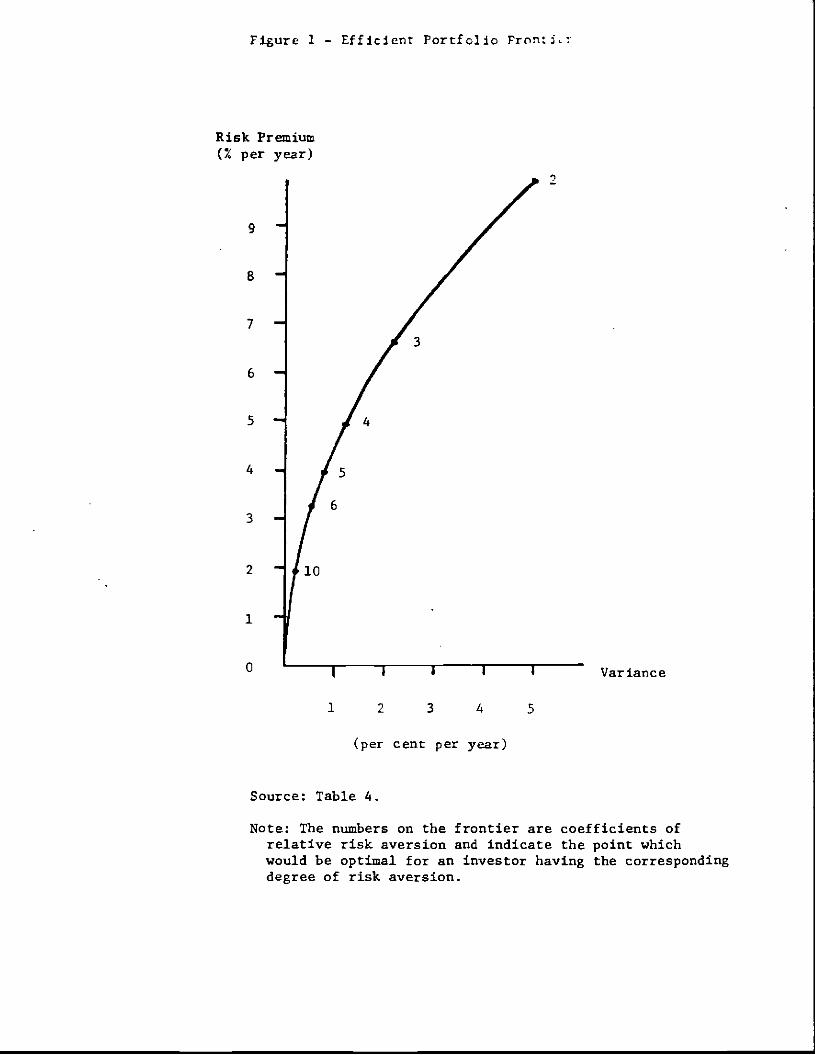
Figure 1 - Efficient Portfolio ProntL

Risk Premium(% per year)

9

8

7

6

5

4

3

2

1

0

(per cent per year)

Source: Table 4.

Note: The numbers on the frontier are coefficients ofrelative risk aversion and indicate the point whichwould be optimal for an investor having the correspondingdegree of risk aversion.

3

4

5

6

10

1 2 3 4 5

Variance

—21—

in bonds of various durations, in order to attain a mean risk premium of 1.95%

per year with a variance of only .21% per year.

Note that for coefficients of relative risk aversion smaller than the

econon—wide average of' 4, the investor takes larger short positions in billsand long positions in stocks and bonds ofmost durations. In the first row, forexample, we see that an investor with a risk aversion coefficient of 2 nearly

doubles the mean risk premium on his portfolio relative to the average investor,but also increases the variance by a factor of four.

Short—selling treasury bills is difficult in practice. This difficulty

can be overcome in two ways. First, a large investment house or pension fund

could allow its less risk—averse investors to short—sell to the more risk—averse

investors, as a purely internal transaction. Second, and more likely, a less

risk—averse investor can simply take a long position in stock market futures as

a way to hold a levered position in stocks.

Table 5 and Figure 2 present our estimates of the welfare loss to an

investor from having his opportunity set restricted to various subsets of the

ten asset classes. The numbers in this table represent the amount of money the

investor would need to be given per $10,000 of his current wealth to make him as

well off with the restricted choice set as he would be with the full set of ten

assets. In order to do these calculations we had to determine the mean rates of

return themselves, not Just the risk premia. We did this by assuming that the

mean on bills is zero and calibrating all other rates accordingly. This assump-

tion was based on the actual mean real return on bills observed over the past 30

years.

Figure 2 — Welfare Loss from incomplete UlversifIcatloit

(1) stocks and bonds ofduration 2 years

- —.(3) stocks, bills and bondsof duration 2 years

I I I I I

2 3 4 5 6

Coefficient of Relative Risk Aversion

Source: Table 5.

(1)

(2)

Welfare Loss

550

500

450

400

350

300

250

200

150

100

50

(3)

(2) stocks and bonds ofduration i year

—22—

We also had to assume a rate of time preference and a specific planning

horizon. We arbitrarily set these at 14% per year and infinity, respectively,

but did a sensittvity analysis which we report below in Table 6. It should be

noted that the infinite horizon assumption is really meant to represent the case

where tine of death is uncertain and the parameter p in (2) incorporates the

rate of nortality as in Merton (1911). Note also that Table 5 shows the welfare

loss from restricting the investor's portfolio choice forever, not just for a

limited period.

Table 5 and Figure 2 show that when the investor is restricted to onlytwo assets, the welfare impact of the restriction can be quite sensitive to his

coefficient of risk aversion, If the two assets are stocks and bonds of duration

2 years (curve 1), we see that the welfare loss is small for an investor with a

risk aversion coefficient equal to the average, 14, but increases sharply on

either side of this value. If, on the other hand, the two assets are stocks and

bonds of duration 1 year (curve 2), then the welfare loss is greatest for the

least risk averse investor, but is not extreri for any investor. Investors with

coefficients of risk aversion equal to 3 or 14 are better off with stocks and

bonds of duration 2 years, whereas investors who are either more or less risk

averse than that would prefer stocks and bonds of duration 1 year.

A coqarison of the first two columns in Table 5 reveals that stocks

and bonds of duration one year are preferable to stocks and bills for all

investors except those with risk aversion of 2. Mving across Table 5 we see

that as the duration of the bond fund increases the welfare loss becomes more

sensitive to the coefficient of risk aversion. Thus for bonds of duration 14

years the smallest welfare loss relative to the full 10 asset opportunity set

occurs at a coefficient of risk aversion of 3, rising quite sharply on either

C

Table 5: Welfare Loss from Incomplete Diversification(dollars per $10,000 of wealth)

2 Assets 3 AssetsCoefficient Stocks, billsof Relative Stocks and Stocks and bonds of duration: and bonds ofRisk Aversion bills lyear 2years Iyears 8years duration 2years

2 $34b $b68 $585 $713 $80b $29

3 279 191 128 65 27

249 77 32 17 162 28

5 231 186 27 2,090 30

6 218 91 592 2,325 6,197 33

Notes: These estimates correspond to an assumed rate of time pre-ference of 14% per year and an infinite horizon. In settingthe mean rates of return we assumed that the nean on bills iszero and calibrated the others accordingly.

—23-.

side of that value and becoming particularly severe for very risk averse

investors.

The last column in Ible 5 shows that when the choice set is expanded

from two to three assets, stocks, bills and bonds of duration two years, the

magnitude of the welfare loss rails dramatically for all investors, regardless

of their degree of risk aversion. Itving these three assets to choose from is

thus almost as good as having all ten.

The effects of changing our assumptions about the rate of time pre—

ference and the horizon are shown in Table 6. The magnitude of the welfare loss

from restricting the choice set to stocks and bills is greater the lower the

rate of time preference and the longer the horizon.

These numerical results suggest that if an employer—sponsored savings

plan is going to restrict its participants to a choice of only two funds, then

since the sponsor does not know the exact degree of risk aversion of the patici—

pants, it would make sense to let the two funds be stocks and bonds of duration

1 or 2 years. If, however, the sponsor is willing to expand the number of funds

to three, then stocks, bills and bonds of duration two years will eliminate

alw,st all of the welfare loss relative to the full ten asset opportunity set.

The applicability of our analysis to employer—sponsored tax—deferred

savings plans is limited by two factors; assets held outside the plan, andtaxes. Without taxes it is trivially obvious that the omission of bills from a

savings plan is of no consequence if investors can hold a money market fund on

their own account. When there are tax advantages to investing in a savings

plan, however, on the margin the investor prefers to hold assets inside the

plan. If the plan fails to offer a full menu of assets, the investor will

Table 6: Effect of Rate of Time Preference andTime Horizon on the Welfare Loss from

Incomplete Diversification(dollars per $10,000 of wealth)

2 Assets:A. Itte of Stocks

time preference and bills

0 $3914

2% per year 305

4% per year 249

Notes: Assumes a coefficient of risk aversion of 4 and an infinitetime horizon.

2 Assets:Stocks

B. Time horizon and bills

1 nDnth $0.28

5 years 11

infinite 2149

Notes: Assumes a rate of time preference of 4% per year.

—2

suffer a welfare loss. Our numerical calculations can be viewed as applying to

a world in which all assets are invested in a tax—deferred savings plan with a

restricted menu of assets. In general, however, our numerical calculations

still provide an upper bound on the possible welfare loss, for the following

reason: if the investor could in principle invest all wealth in the plan, and

chooses not to do so, in order to diversify, then the welfare loss must be less

than for an investor who is (as in our calculations) constrained to hold only

those assets offered by the plan.

In practice, of course, additional complications reduce the importance

of tax—deferred savings plans. The IRS imposes a limit on the contributions to

these plans, and frequently there are penalties or delays associated with the

Dreunture withdrawal of funds. These considerations will reduce the percentage

of an investor's wealth s.thich is held in such savings plans. Therefore the

failure of the plan to offer certain assets is less important, since freely

chosen assets held outside the plan will undo the effect of restrictions imposed

within the plan. Our numerical estimates again provide an upper bound on the

welfare loss.

—25—

V. Shadow Riskiess Rates and the Welfare Gain from Introduction of a Riskless

Real Asset

In part II we defined the shadow riskless rate of interest as that rate

at which an investor would have a zero gain in welfare from havIng his choice

set expanded to include an asset which was riskless in real terms. Equation

(12) showed that this rate is below the mean real rate of return on the minimum

variance portfolio by an amount equal to the investor's degree of relative risk

aversion tints the variance of the minimum variance portfolio. Given that our

estinnte of this variance is a mere .Oiblt% per year, it follows that even a veryrisk averse investor (6 = 6) would be willing to give up less than 9 basis

points.

Since the avera€e degree of risk aversion is b, if a market for

riskless real bonds could be established costlessly, the market clearing real

interest rate would be about 6 basis points below the mean rate on the mininum

variance portfolio. Th,ble 7 shows what the welfare gain would be to investors

with varying degrees of risk aversion.

The magnitude of the welfare gain to investors does not appear to be

large. The numbers in the first column of Thble 7 show the results obtained

using the actual covariance matrix estimated for the 1913—1981 subperiod. The

second column shows the results of an experiment in which we made all nominal

debt securities twice as risky by doubling their variances and covariances,

leaving the variance of stocks unchanged. While the effect is to approximately

double the welfare gain to investors at any degree of risk aversion, the magni-

tude of the gain still appears small.

Table T: Welfare Gain from Introduction of a Real RisklessAsset (dollars per $10,000 of wealth)

Welfare GainCoefficient of ActualRelative Risk Covariance Double all variances &

Aversion F'htrix covariances but, stocks

2 $32 $63

3 1 13

4 0 0

5 6 12

6 25 149

—26—

These results suggest one possible reason for the nonexistence of index

bonds in the U.S. capital market. Since there would probably be some costs

associated with creating a new market for such bonds, the benefits would have to

exceed those costs. Given the assumptions of our model, in particular the

assumption of homogeneous expectations, the benefit from trading in index bonds

would have to arise from differences in the degree of risk aversion among

investors. If as Table 7 suggests, the welfare gain does not appear to be large

over a fairly broad range of risk aversion coefficients, then one should not be

surprised at the failure of a market for index bonds to appear.

One should bear in mind that Table 7 is derived assuming a zero net

aggregate supply of index bonds. Thus it does not answer the question of

whether the welfare gain from indexing government debt would be significant.

—27—

VI. Summary and Discussion of Findings

We undertook this research with two main policy questions in mind: Ci)

Is there a significant welfare loss stemming from the practice on the part of

many employer—sponsored savings plans of restricting a participant's choice of

investments to two or three asset classes? (2) What is the potential welfare

gain from the introduction of trading in privately issued index bonds? In this

section we summarize and discuss the implications of our findings for each.

With regard to the first of these, we have shown that there is no

necessary loss of welfare from restricting an investor' s choice set to only two

funds, provided these two are properly chosen. If they are the market portfolio

and the xniniraim variance portfolio, then there will be no loss at all. In prac-

tice, however, many plans offer a diversified common stock fund and an

interdiate—ten fixed—interest bond fund as the only two assets, and in such

cases there can be a substantial welfare loss to participants whose degree of

risk aversion differs appreciably from the average. ?tst of this loss can be

eliminated for risk averse participants by introducing as a third option a money

market fund.

With regard to the second question, our results indicate that the

potential welfare gain from the introduction of index bonds in the current U.S.

capital market is probably not large enough to justify the costs of innovation.

The major reason for the small gain we calculate is the fact that one month

bills with their small variance of real returns are an effective substitute for

index bonds.

There are some important factors bearing on these two policy questions,

which we either excluded or ignored in our analysis, and we need to at least

—28—

consider their potential impact on our conclusions. The first is the fact that

we limited ourselves to onJj a subset of the assets which individuals in the

U.S. hold in their portfolios. Specifically, we excluded residential real

estate, consumer durables, and nontradeable assets like human capital and social

security wealth.

UndoubtedJj the inclusion of these other assets would affect the nagni—

tude of the welfare effects we calculated. Thus the welfare loss to an indivi-

dual whose employer—sponsored savings plan offers only a stock fund and a bond

fund would almost surely be smaller. The loss would appear smaller still, were

we to take into account the fact that individuals have access to other assets

outside of the plan. Nonetheless, it is probably still true to say that not

having a money market option lowers the welfare of investors who are more risk

averse than the average. Similarly, the swall welfare gain from index bonds,

which we calculated, would probably become even smaller, in the context of the

broader spectrum of assets, especially when one considers that Social Security

is indexed.

Our agenda for future research starts with a more detailed quantitative

analysis of the impact of these additional assets.

—29—

Footnotes

1. An example of particular relevance to academics is the plan managed by theTeachers Insurance and Annuity Association and offered by mary privateeducational institutions in the U.S. Under this plan the participant canchoose between a common stock fund, the College Retirement Equities Fund(CREF), and a second fund which is essentially a portfolio of intermediateterm nominal bonds.

2. See, for example, the paper by Fischer (1915) and the references citedtherein.

3. All of these simplifying assumptions are, of course, counterfactual, andthere is a considerable literature on the effect of relaxing each of them.The only one which we think would materially affect the main results inthis paper is the no taxes assumption. We discuss its likely effects insection IY, p. 23.

4• A necessary condition for (!) to be correct is p > iv. See Merton (1969).

5. Pratt (l964) shows that for small changes in wealth this insurance premiumis approximately 1J26x . Note that x2 is the variance of the proportionalchange in wealth caused by the risky prospect.

6. See Bodie (1982) for a discussion in terms of nominal rates of return andunanticipated inflation.

7. Note that if >0 then as 1-I + equation (12) reduces to:

'S

(12') —(

8. Duration, as defined by Macaulay (1938) is a weighted average of the yearsto naturity of each of the cash flows from a security. The weights arethe present value of each year's cash flow as a proportion of the totalpresent value of the security. Duration equals final maturity only in thecase of pure discount bonds. For coupon bonds and mortgages, duration isalways less than maturity. The difference between maturity and durationfor ordinary coupon bonds and mortgages is greater the longer the finalmaturity and the higher the level of interest rates. In our sample ofbonds this difference rose steadily over the 1953—1981 period due to therising trend in interest rates. The most pronounced differences were inthe 8 year duration category. In 1953 the average maturity of the bondsin our 8 year duration portfolio was just under 9 years whereas in 1981the average maturity of the 8 year duration portfolio was 23 years. Thisvariation over the last 30 years calls into question the appropriatenessof a bond return series with a constant maturity of 20 years, such as theone tabulated by Ibbotson and Sinquefield (1982).

—30—

9. For the arguments on both sides of this debate see Barro (19Th) and Ibbin(1980).

10. Including residential real estate would raise another theoretical issue.Individual holdings of residential real estate serve both to diversify theportfolio and to hedge against changes in the relative price of housingservices. This hedging denand is ignored in our model and including itwould substantially increase the difficulty of solving for the J function.

11. Equation (9) in our model implies that:

2(a. —a.)

R.—R = 'H nan (B -R1 win 2 2 H mm(a — a .

M win

Since a2 is very small relative to the covariance of stocks with themarket and to the variance of the market, we get:

-B. (B —R )stocks win stocks t4 win

—31—

References

Barro, B. l974. Are Government Bonds Net Wealth? Journal of Political Fcononr.

Bodie, Z. 1982. Inflation Risk and Capital Market Equilibrium. The FinancialReview. May.

Fischer, S. 1975. The Demand for Index Bonds. Journal of Political Econorg,r.June.

Friend, I. and Blume, M. 1975. The Demand for Risky Assets. American EconomicReview. December.

Friend, I. and Hasbrouck, J. 1982. Effect of Inflation on the Profitabilityand Valuation of U.S. Corporations. Proceedings of the Conference onSavings, Investment and Capital Markets in an Inflationary Environment,

Szego and Sarnat, eds., Ballinger, 1982.

Grossman, S. and Shiller, B. 1981. The Determinants of the Variability ofStock Market Prices. American Economic Review. May.

Ibbotson, R.G. and Sinquefield, R.A. 1982. Stocks, Bonds, Bills and Inflation.

Macaulay, F.R. 1938. Some Theoretical Problems Suggested by the Movcernente ofInterest Rates, Bond Yields, and Stock Prices in the U.S. since 1856.New York: National Bureau of Economic Research.

Markowitz, 11. 1952. Portfolio Selection. Journal of Finance. March.

Merton, B.C. 1969. Lifetime Portfolio Selection Under Uncertainty: TheContinuous—Time Case. Review of Economics and Statistics. August.

____________ 1971. Optimum Consumption and Portfolio Rules in a Continuous—Time Model. Journal of Economic Theory. December.

____________ 1972. An Analytic Derivation of the Efficient Portfolio Frontier.Journal of Financial and Quantitative Analysis. September.

___________ 1980. On Estimating the Expected Return on the Market: AnExploratory Investigation. Journal of Financial Economics. December.

Pratt, J.W. 19614. Risk Aversion in the Small and in the lArge. Econometrica.

Tobin, J. 1980. Asset Accumulation and Economic Activity. University ofChicago Press.