Zoltan Zs´ oka´ - BME-HITzsoka/kutat/thesis/dissz.pdf · es Gazdas´ agtudom´ ´anyi Egyetem...
113
Budapest University of Technology and Economics Department of Telecommunications Zolt´ an Zs ´ oka Performance modelling and analysis of IP over WDM networks Scientific supervisors: Dr. L´ aszl´ o Jereb and Dr. Renato Lo Cigno
-
Upload
hoangkhuong -
Category
Documents
-
view
214 -
download
0
Transcript of Zoltan Zs´ oka´ - BME-HITzsoka/kutat/thesis/dissz.pdf · es Gazdas´ agtudom´ ´anyi Egyetem...

Budapest University of Technology and Economics
Department of Telecommunications
Zoltan Zsoka
Performance modelling and analysis of IP overWDM networks
Scientific supervisors:
Dr. Laszlo Jereb and Dr. Renato Lo Cigno

The reviews of the dissertation and the report of the thesis discussion are available at the
Dean’s Office of the Faculty of Electrical Engineering and Informatics of the Budapest
University of Technology and Economics.
Zoltan Zsoka, 2005

Budapesti Muszakies Gazdasagtudomanyi Egyetem
Hıradastechnikai Tanszek
Zsoka Zoltan
Teljesıtmeny-modellezeses elemzes IP over WDMhalozatokban
Konzulensek:
Dr. Jereb Laszlo es Dr. Renato Lo Cigno

Az ertekezes bıralatai es a vedesen keszult jegyzokonyv elerheto a Budapesti Muszaki
es Gazdasagtudomanyi Egyetem Villamosmernoki es Informatikai Karanak Dekani Hi-
vatalaban.
Zsoka Zoltan, 2005

Contents
1 Introduction 1
1.1 Motivation . . . . . . . . . . . . . . . . . . . . . . . . . . . . . . . . . . 1
1.2 Main issues . . . . . . . . . . . . . . . . . . . . . . . . . . . . . . . . . 2
1.3 Organisation and content of this dissertation . . . . . . . .. . . . . . . . 2
2 Problems and methods 4
2.1 General model of the network structure . . . . . . . . . . . . . . .. . . 4
2.2 Decomposition of the analysis task . . . . . . . . . . . . . . . . . .. . . 7
2.3 Analysis of theoptical layer . . . . . . . . . . . . . . . . . . . . . . . . 8
2.3.1 WDM technology . . . . . . . . . . . . . . . . . . . . . . . . . . 9
2.3.2 Optical connection requests . . . . . . . . . . . . . . . . . . . . 9
2.3.3 Performance of dynamic WDM networks . . . . . . . . . . . . . 11
2.4 Studies of thedata layer . . . . . . . . . . . . . . . . . . . . . . . . . . 11
2.4.1 Model of the IP network and its traffic . . . . . . . . . . . . . . .12
2.4.2 Performance of QoS routing solutions . . . . . . . . . . . . . .. 13
2.5 Analysis of the multilayer network . . . . . . . . . . . . . . . . . .. . . 16
2.5.1 Modelling IP over WDM . . . . . . . . . . . . . . . . . . . . . . 16
2.5.2 Dynamic grooming techniques . . . . . . . . . . . . . . . . . . . 17
2.5.3 Performance of dynamic grooming . . . . . . . . . . . . . . . . 17
2.6 Approaches . . . . . . . . . . . . . . . . . . . . . . . . . . . . . . . . . 19
2.6.1 Performance measures in networks . . . . . . . . . . . . . . . . 19
2.6.2 Performance modelling with theoretical methods . . . .. . . . . 20
2.6.3 Simulation tools . . . . . . . . . . . . . . . . . . . . . . . . . . 21
I
CONTENTS
2.6.4 Application of the methods . . . . . . . . . . . . . . . . . . . . . 22
3 Studies at theoptical layer 27
3.1 Introduction . . . . . . . . . . . . . . . . . . . . . . . . . . . . . . . . . 27
3.2 Theoretical analysis of dynamic WDM networks . . . . . . . . . .. . . 28
3.2.1 Description of the computation model . . . . . . . . . . . . . .. 31
3.2.2 Complexity of the algorithm . . . . . . . . . . . . . . . . . . . . 35
3.2.3 Numerical results . . . . . . . . . . . . . . . . . . . . . . . . . . 36
3.3 Discussion . . . . . . . . . . . . . . . . . . . . . . . . . . . . . . . . . . 40
4 Performance of thedata layer 42
4.1 Introduction . . . . . . . . . . . . . . . . . . . . . . . . . . . . . . . . . 42
4.2 Evaluation of routing algorithms in the Internet . . . . . .. . . . . . . . 43
4.2.1 Motivation . . . . . . . . . . . . . . . . . . . . . . . . . . . . . 43
4.2.2 Basic assumptions . . . . . . . . . . . . . . . . . . . . . . . . . 44
4.2.3 Modelling elastic traffic connections . . . . . . . . . . . . .. . . 46
4.2.4 Formulation of the routing algorithms . . . . . . . . . . . . .. . 49
4.2.5 Comparison ofTB andDB approaches . . . . . . . . . . . . . . . 53
4.3 Networks with stale link state information . . . . . . . . . . .. . . . . . 59
4.3.1 Information distribution . . . . . . . . . . . . . . . . . . . . . . 60
4.3.2 Model and problem formulation . . . . . . . . . . . . . . . . . . 61
4.3.3 Simulation Results . . . . . . . . . . . . . . . . . . . . . . . . . 62
4.4 Novel QoS routing strategies . . . . . . . . . . . . . . . . . . . . . . .. 65
4.4.1 Multimetric Sequential Filtering algorithms . . . . . .. . . . . . 66
4.4.2 Formal description . . . . . . . . . . . . . . . . . . . . . . . . . 67
4.4.3 Routing based on Network Graph Reduction . . . . . . . . . . . 72
4.5 Discussion . . . . . . . . . . . . . . . . . . . . . . . . . . . . . . . . . . 78
5 Analysis of dynamic grooming 81
5.1 Introduction . . . . . . . . . . . . . . . . . . . . . . . . . . . . . . . . . 81
5.2 Grooming guaranteed traffic . . . . . . . . . . . . . . . . . . . . . . . .82
5.2.1 Considered traffic model and grooming scheme . . . . . . . . .. 83
5.2.2 Description of the model . . . . . . . . . . . . . . . . . . . . . . 84
II

CONTENTS
5.2.3 Numerical results . . . . . . . . . . . . . . . . . . . . . . . . . . 84
5.3 Grooming elastic traffic . . . . . . . . . . . . . . . . . . . . . . . . . . .85
5.3.1 Considered models and schemes . . . . . . . . . . . . . . . . . . 86
5.3.2 Performance measures . . . . . . . . . . . . . . . . . . . . . . . 88
5.4 Discussion . . . . . . . . . . . . . . . . . . . . . . . . . . . . . . . . . . 93
6 Conclusion 95
III

LIST OF ACRONYMS
List of Acronyms
ASON Automatic Switched Optical Network
CAC Connection Admission Control
CBR Constant BitRate traffic
DB Data-Based traffic model
FSP Fixed Shortest Path routing
G-OXC Grooming OXC
HGGM Homogenous Guaranteed-traffic Grooming Model
IP Internet Protocol (Network)
ISP Internet Service Provider
LD Load Dependent routing
MD Minimum Distance routing
MLLC Multifiber Link-Load Correlation
MPLS Multi-Protocol Label Switching
MSF Multimetric Sequential Filtering
NGR Network Graph Reduction
OADM Optical Add-Drop Multiplexer
OXC Optical Crossconnect
QoS Quality of Service
ROADM Reconfigurable Optical Add-Drop Multiplexer
RWA Routing and Wavelength Assignment
SLA Service Level Agreement
SW Shortest-Widest routing
TB Time-Based traffic model
TCP Transmission Control Protocol
UDP User Datagram Protocol
WDM Wavelength Division Multiplexing
WDMM Wavelength Dependent Multifiber Model
WS Widest-Shortest routing
IV

Chapter 1
Introduction
1.1 Motivation
Networking is one of the most important challenges of the information society evolving
in our days. The fast and safe transfer of sometimes huge amount of data is at the heart
of current applications. The communication among the members of a population of users
is indispensable in the modern working processes based on knowledge shared by users
often geographically scattered.
A very important objective in the design and operation of telecommunication net-
works is the effective use of the available resources. A characterising factor of this
efficiency is thegeneral routing problemboth in virtual circuit switched or in packet
switched networks.
A very relevant decision of the network provider is the selection of the most suitable
solution and its operation in his system. The support of the performance analysis is
essential both in the network design and in monitoring tasks. Its role becomes even more
important if any component of the system works in a dynamic manner.
The analysis of thegeneral routing problemincluding the route selection on a given
topology and some technology-dependent tasks like wavelength assignment, grooming
etc., needs rather complex performance studies. Several previous works on these issues
have been presented in recent years, introducing new algorithms, analysing and compar-
ing them with different tools and methods, e.g., [1, 2, 3, 4, 5].
1
INTRODUCTION
The main objective of the dissertation is to provide new methods and present re-
sults regarding the routing-dependent performance capabilities of optical and IP-based
networks, that play determining role in telecommunicationservices of today and of to-
morrow.
1.2 Main issues
The general routing includes mechanisms that may work in different network layers and
consider different aspects in their decisions. We worked onthree specific fields; each of
them is strictly joint to the general problem of routing analysis in IP over WDM networks:
• performance analysis of dynamically switched optical networks,
• comparison of existing, and development of new routing algorithms used in IP
networks,
• studies on the cooperation of theoptical and theelectronic layers, i.e., traffic
grooming issues.
In different network scenarios technology and traffic characteristics pose limits to the
methods that can be applied.
1.3 Organisation and content of this dissertation
The dissertation consists of five more chapters. Chapter 2 specifies the problems that we
studied. Starting from a general description of the networkenvironment it presents the
related questions that arise in the performance analysis task. The approaches that can be
applied in the studies are briefly presented. Their benefits and drawbacks is discussed
from the point of view of the specific scenarios.
The results are organised according to the studied subproblems listed above. For all
discussed subproblems, first a description of the network model and a short summary of
the related works are given, then the solution of the subproblem is presented, illustrated
with numerical results and shortly discussed.
2
INTRODUCTION
Chapter 3 includes the achievements in the field of the theoretical analysis of auto-
matically switched optical networks with dynamic optical channel requests.
In Chapter 4 the studies on the flow level analysis of elastic IPtraffic in different
network architectures are presented. New routing algorithms are introduced and analysed
with simulation showing their benefits and drawbacks.
Chapter 5 deals with the analysis of dynamic grooming of lowerspeed traffic on op-
tical channels. A theoretical solution is given for the caseof guaranteed traffic and some
elementary studies are presented for the case of a more complex model that considers
elastic traffic.
Finally, Chapter 6 summarises and concludes the thesis, mentioning some possible
directions of further studies.
3

Chapter 2
Problems and methods
In the previous chapter we presented the motivations that lead us to examine the general
routing issues in networks from the performance point of view. Now we define more
precisely the problems we wanted to solve. We also list and classify the methods that can
be applied in the analysis.
2.1 General model of the network structure
Among the fix, cable based, non-local telecommunication architectures presently used for
networking, the one with the brightest perspectives is the TCP/IP based internetworking
over static or dynamic wavelength division multiplexed optical networks. We study IP
over WDM in the core segment of the network, assuming a WAN or MAN environment.
According to the network model presented in [6] and without specifying the service
model we define two layers, that compose the network:
• the optical layerprovides high capacity connectivity by establishing optical con-
nections that may span large physical distances,
• thedata layerprovides resources and networking functions to the user applications
that can use several transport protocols.
The optical layercan be interpreted as a network that consists of optical links and
switching nodes. The optical links contain several fibers, their number can go up to
4

PROBLEMS AND METHODS
hundreds in one link. Each fiber can transport data on severalwavelengths. A wavelength
realises a high capacity optical channel on the link.
The nodes model optical cross-connects, OXCs with optional traffic adding and drop-
ping functions as in OADMs and ROADMs. Some switching devices allow subchannel
bundling based on timeslots. If this capability is available in the network we can define
subwave channelson the links. The capacity of these optical channels is a fraction of the
wavelength capacity. The nodes can have different capabilities of wavelength conversion
and timeslot reordering. The latter realises the conversion of thesubwave channel. There
are two extreme architectures from this point of view: in thefirst full conversion is pos-
sible at each node and in the other neither wavelength norsubwave channelconversion
is enabled.
A connection through a contiguous series of optical channels with equivalent capac-
ity is calledlightpath. It is established according to the RWA algorithm and the switch-
ing capabilities in the nodes, and it provides high bandwidth connectivity between its
endpoints. There can be established more parallellightpathsbetween any source and
destination node pairs.
The main resources in thedata layerare the routers in the nodes and the links pro-
viding bandwidth capacity for both guaranteed or best effort type user traffic. The most
important functions of the routers are routing and queue management, including buffer-
ing capabilities. In order to take always the right decisions, these devices observe the
traffic on the links and advertise among them the data collected on the network status.
Since the capacity of alightpath is of several Gbps and users require bandwidths that
are orders of magnitude smaller, the multiplexing of IP traffic on the optical channels is
mandatory. This is the basic motivation of grooming.
In some of the network nodes there are special switching equipments that are neces-
sary to harmonise the tasks of both layers and to perform the data transfer among them.
The compound architecture of these nodes consist of one or more cooperating physical
devices. User traffic reaches theoptical layer through interlayer channelsestablished
via grooming ports. The number of these ports limits the number of parallelinterlayer
channels. In our studies we have assumed infinite number of grooming ports in each
node.
The logical connection between the layers of our model is themapping of thelight-
5
PROBLEMS AND METHODS
paths to the links of thedata layer topology. Since these links exist only during the
lifetime of optical connections, they are virtual links from the network point of view, but
the entities of thedata layersee them as normal links. The virtual links form the virtual
topology that can change dynamically if theoptical layeris dynamically reconfigurable.
This indicates, that the topology of thedata layerdiffers from the topology of theoptical
layer.
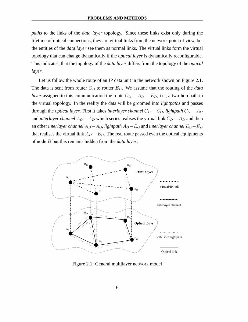
Let us follow the whole route of an IP data unit in the network shown on Figure 2.1.
The data is sent from routerCD to routerED. We assume that the routing of thedata
layer assigned to this communication the routeCD − AD − ED, i.e., a two-hop path in
the virtual topology. In the reality the data will be groomedinto lightpathsand passes
through theoptical layer. First it takesinterlayer channelCD − CO, lightpathCO − AO
andinterlayer channelAO −AD which series realises the virtual linkCD −AD and then
an otherinterlayer channelAD−AO, lightpathAO−EO andinterlayer channelEO−ED
that realises the virtual linkAD −ED. The real route passed even the optical equipments
of nodeB but this remains hidden from thedata layer.
AD
� �� �� �
� �� �� �
� �� �� �
� �� �� �
� �� �� �
� �� �� �
� �� �� �
� �� �� �
� �� �� �
� �� �� �
� �� �� �
� �� �� �
� �� �� �
� �� �� �
� �� �� �
� �� �� �
� �� �� �
� � � � � � �� � � � � � �� � � � � � �� � � � � � �� � � � � � �� � � � � � �� � � � � � �� � � � � � �� � � � � � �� � � � � � �� � � � � � �
� � � � � � �� � � � � � �� � � � � � �� � � � � � �� � � � � � �� � � � � � �� � � � � � �� � � � � � �� � � � � � �� � � � � � �� � � � � � �
� � � � � � � � �� � � � � � � � �� � � � � � � � �� � � � � � � � �� � � � � � � � �� � � � � � � � �� � � � � � � � �� � � � � � � � �� � � � � � � � �
� � � � � � � � �� � � � � � � � �� � � � � � � � �� � � � � � � � �� � � � � � � � �� � � � � � � � �� � � � � � � � �� � � � � � � � �� � � � � � � � �
� � � � � � � � � � � �� � � � � � � � � � � �� � � � � � � � � � � �� � � � � � � � � � � �
� � � � � � � � � � � �� � � � � � � � � � � �� � � � � � � � � � � �� � � � � � � � � � � �
� � � � � � � � � � � �� � � � � � � � � � � �� � � � � � � � � � � �� � � � � � � � � � � �
� � �� � �� � �� � �� � �� � �� � �� � �� � �� � �� � �� � �� � �
� � �� � �� � �� � �� � �� � �� � �� � �� � �� � �� � �� � �� � �
� �� �� �� �� �� �� �� �� �� �� �� �� �� �� �� �� �� �� �
� �� �� �� �� �� �� �� �� �� �� �� �� �� �� �� �� �� �� �
Optical Layer
Data Layer
Established lightpath
Optical link
Virtual/IP link
O
D
D DD
D
DO
EOO
B
CE
BO
A
C
Interlayer channel
Figure 2.1: General multilayer network model
6

PROBLEMS AND METHODS
We discuss later the technologies and traffic types that characterise this multilayered
model. Figure 2.1 presents the data planes of the two layers and the connection between
them. Control plane details are neglected in this abstraction of IP over WDM networks1
and we assume a single-domain environment in both layers.
2.2 Decomposition of the analysis task
The main objectives of the studies presented in the dissertation is to find the right per-
formance measures that characterise the modelled networksand to evaluate them consid-
eringgeneral routing problemsolutions. The optimal solution would be the compound
analysis of the multilayer network architecture, but beside the very complex modelling
task, this meets with other difficulties too. On the one hand the different layers imply dif-
ferent characteristics to observe. The different issues may require also different methods
to apply in the analysis.
On the other hand thegeneral routing problemmay include multiple functions, thus
enlarges also the solution space to study. Using a compound model the separation of the
effects caused by each cooperating function becomes rathercomplex. For instance, the
effects of the current IP network routing may blend with thatof the applied wavelength
assignment and lead to a confusion in the analysis.
We focus the analysis on the special issues in a more effective way by decomposing
the network and observing the layers separately. The performance of not compound
routing functions can be analysed easier this way, since it remains tractable how the
algorithm settings affect the behaviour of the network. However, there are questions
that refer the issues of the cooperation of the layers and thecompound analysis is surely
indispensable, e.g. the performance of a given grooming solution.
Figure 2.2 illustrates the decomposition of the IP over WDM architecture. In the
compound model data transfer requests arrive from the IP users to the network. The
changes of the traffic generated by the service of the user requests implies requests to
opening or closing optical connections, i.e.,lightpaths, according to the decisions of the
grooming policy.
1GMPLS is a possible choice for signaling.
7

PROBLEMS AND METHODS
t
t
t
t
� �� �� �� �
����
����
����
� �� �
��
��
����
����
� �� �
��
� �� �
��
����
����
� �� �� �� �
� �� �
��
� �� �� �� �
!!
""##
$ $$ $
%%
& && &' '' '
( ( ( (( ( ( (( ( ( (( ( ( (( ( ( (( ( ( (
) ) ) )) ) ) )) ) ) )) ) ) )) ) ) )) ) ) )
* * * * ** * * * ** * * * ** * * * ** * * * *
+ + + + ++ + + + ++ + + + ++ + + + ++ + + + +
, , , , , , , ,- - - - - - -
. . . . . . . .
. . . . . . . ./ / / / / / // / / / / / /
0 00 00 00 00 00 00 0
1 11 11 11 11 11 11 1
2 22 22 22 22 22 22 22 22 22 2
3333333333
4 4 4 44 4 4 44 4 4 44 4 4 44 4 4 44 4 4 4
5 5 5 55 5 5 55 5 5 55 5 5 55 5 5 55 5 5 5
6 6 6 6 66 6 6 6 66 6 6 6 66 6 6 6 66 6 6 6 6
7 7 7 7 77 7 7 7 77 7 7 7 77 7 7 7 77 7 7 7 7
8 8 8 8 8 8 8 89 9 9 9 9 9 9 9
: : : : : : : :: : : : : : : :; ; ; ; ; ; ; ;; ; ; ; ; ; ; ;
< << << << << << << <
= == == == == == == =
> >> >> >> >> >> >> >> >> >> >
? ?? ?? ?? ?? ?? ?? ?? ?? ?? ?
Optical LayerOptical Layer
Data Layer
Data Layer
Requests in IP over WDM Requests in IP
Requests in WDM
Figure 2.2: Separation of network layers
If we separate the layers, only the relating requests and functions need to be con-
sidered in their models. This simplifies the analysis.The decomposition of our general
analysis task results in three subproblems:
• analysis of theoptical layeras a WDM network with fix topology,
• analysis of thedata layeras an IP network with fix topology,
• analysis of the IPoWDM network with fix topology in theoptical layerbut with
variable topology in thedata layer.
The following three sections deal with these three cases, introducing also the joint
issues and presenting more details on the suitable models ofthe offered traffic.
2.3 Analysis of theoptical layer
The bottom-up fashion exploring of the IP over WDM network implies first the observa-
tion of the optical network layer.
8

PROBLEMS AND METHODS
2.3.1 WDM technology
Wavelength division multiplexing network architecture isone of the most effective trans-
port networking solution of our days [7]. In these optical switching networks the capac-
ity granularity is the optical channel that is physically realised as a lightbeam of a given
wavelength in a fiber. This means a connection of several Gbps. Since WDM technology
allows the use of several beams of different wavelengths in the fibers, the capacity of a
fiber is greater than1 optical channel. Optical links can contain several fibers realising
the multifiber environment.
A recent research and development area in the telecommunication field is the inves-
tigation of WDM networks that support dynamic reconfiguration, e.g., ASON [8, 9].
These networks treat dynamically arriving optical connection requests. On the one hand,
the motivation of dynamics is to provide services with higher utilisation of optical net-
work resources. On the other hand, this solution provides higher performance to the cus-
tomers, since their resource needs can be satisfied dynamically and only the real usage
of resources has to be payed. Optical channel provisioning allows end to end lightpath
composition.
As it can be expected, the efficiency of such services dependsstrongly on the wave-
length conversion capability [3], since without converters only the identical wavelengths
of links can be connected in alightpath. Not considering the technology differences, hav-
ing full wavelength conversion in all nodes of the network reduces the problem. The issue
is similar to that of a simple circuit switched network with very large capacity resources
and high bandwidth requests.
The general case, i.e., the multifiber optical networks withlimited wavelength con-
version capabilities must be modelled in a rather complex way because of the link and
wavelength utilisation dependencies [10].
2.3.2 Optical connection requests
In the case of optical connection requests we cannot make theassumptions typically
used for the traffic of connection oriented networks. The provision of connections with
the bandwidth of a whole optical channel for the traffic of a single IP user is not realis-
tic. However, users with large traffic, e.g. Internet Service Providers may request large
9

PROBLEMS AND METHODS
bandwidth connections and they can be considered as users oftheoptical layer. The data
that the optical users want to transport comes from the aggregation of the traffic of users
in thedata layer. According to the decomposition of the IP over WDM architecture, also
the entities that perform grooming decisions are modelled as optical users.
The characteristics of the requests are not obvious to modelsince the decision to set
up a new optical channel depends strongly on the traffic of theupper layer and on the
applied multiplexing-grooming policy. However, we can recognise two important types
of traffic in the network that can be modelled in a tractable way.
One is the traffic of a static WDM network in the first phase of theprogress towards on
demand provisioning: the permanently provided channels can be torn down if no traffic is
transported on them. A possible mathematical model of this traffic is theBinomialarrival
process with a finite numbern of generators that are able to generate optical connection
requests. Each generator can have zero or one open connection, thus modelling an arrival
process of anM/M/n/n/n system when the ON and OFF periods are with exponentially
distributed length.
The other traffic is present in scenarios with bursty traffic,streaming from overflows
on resources in thedata layerrealised as permanently provided connections in theoptical
layer. Imagine an ISP that has overloaded resources, needs further high capacity links
and thus requests an optical connection. This traffic type can be modelled by thePascal
or negative binomialarrival process that generates requests in a more bursty fashion
[11, 12].
Obviously we can not assume a very large population of independently acting optical
users and thus the classicPoissonarrival model fails in this scenario. However, it can
be used as a good reference point, also because of its popularity. It assumes exponential
distribution for the interarrival time of the connection requests and the connection dura-
tion is a random variable with exponential distribution. Inthe case of aPoissonarrival
process the number of connection requests arrived in a givenperiod of∆ has the peaked-
nessZ = σ2[N ]/E[N ] = 1. Z is less than1 for theBinomialmodel and greater than1
for Pascalprocess.
These traffic models were compared in [13]. In our studies we have not considered
more complex, e.g. PH-based, models for the interarrival process of optical channel
requests. The service time was assumed to have exponential distribution that models a
10

PROBLEMS AND METHODS
memoryless service process.
The connection requests in theoptical layerare very different from the traditional
requests that come from traditional users. In the considered model of IP over WDM net-
work these requests come from the IP control plane when the grooming policy demands
to set up a new virtual link. However, in many cases the communication in thedata layer
can be performed also on the current virtual topology. Thus,the refusion of an optical
connection request does not imply necessarily the blockingof the traffic of IP users and
does not affect critically the data transport service. Considering grooming we can allow
for the optical connection requests a higher blocking probability value than that usual in
PSTN networks.
2.3.3 Performance of dynamic WDM networks
Though there are some relevant differences, the obvious similarities with classic circuit
switched networks suggest us to study similar performance measures as in that research
field. Such measures are the utilisation of the total networktransfer capacity, that of indi-
vidual links and blocking probability, i.e., the ratio of refused optical connection requests.
These quantities represent the cost-efficiency and availability of services provided by the
dynamically switched optical network, thus our studies were focused on the analysis of
these measures.
We dealt mainly with the blocking probability and the impactof the following special
properties:
• wavelength conversion constraints in nodes,
• links consisting of several fibers,
• special traffic models for the requests.
2.4 Studies of thedata layer
Assuming the separation of layers, the analysis of the IP data transport issues becomes
less complex and more tractable. Let us present now the considered model of thedata
layerand the related problems.
11
PROBLEMS AND METHODS
2.4.1 Model of the IP network and its traffic
Our main objective in this area is to study the performance ofrouting algorithms and for
this sake we consider a rather simplified model of the IP network architecture.
The network topology consists of switching nodes and links that connect them. At
this point we do not deal with topology changes. The nodes represent entities realis-
ing routing functionalities, they are entry and exit pointsof traffic and connect adjacent
links. Links represent transporting elements with arbitrary finite capacity that carry data.
Through the constraining effect coming from the finite capacity, they influence strongly
the results of decision mechanisms.
We can consider the network management functions realised by a system of distrib-
uted decisions using information that are available about the whole network. Information
on current utilisation of resources, however, is prone to error measurements, and, most of
all, it quickly becomes outdated. Since thedata layerdoes not include the model of the
control plane of the IP network, we do not consider its technology details and the control
traffic.
IP networks are packet based and originally without providing quality of service guar-
anties. However, architectures that provide QoS for IP users, like MPLS-based services
IntServ [14] or DiffServ [15] emerge more and more with the increase of traffic com-
ing from application with real time transport demands. Though classic IP is a strictly
datagram packet switched architecture, applying these techniques we can identify data
pieces belonging to the same session [16]. We can model the traffic generated by a user
session with adata flow, allowing a more efficient analysis of routing effects on thequal-
ity. A flow can also refer to a set of connections sharing the same source and destination
nodes and having the same QoS requirements. The way a flow is identified within the
network, or whether a flow of packets is a single logical connection or an aggregation of
connections, do not influence basic study results concerning routing performance.
Requests with a data amount to transport arrive to the networkfrom the users accord-
ing to predefined arrival processes. During the processing of a request an indispensable
step is the routing: a path has to be selected that can carry the data of the flow.
According to the flow-based concept routers in our model do not operate on traffic
units smaller than data flows, i.e., the implementation of any packet level function is not
12

PROBLEMS AND METHODS
required. Thus, the model does not consider packet losses and we assume no switching
capacity restrictions in routers, the only limiting factoris the capacity of the IP links.
Users may require guarantees on the service quality or – as more typical in the IP
networks – they may generatebest efforttraffic. In this latter case, the interaction of
flows concurrently transporting on a link leads to elastic rate behaviour, i.e., each flow
achieves a transport rate that depends on the actual networkstate and on the coexisting
flows. The properties of the elastic traffic and the mutual effects of the flows on each
other were analysed in many works, e.g., in [16, 17, 18, 19].
In addition, the model of thedata layerconsiders the concept offlow starvation.
Caused by the lack of admission control, the number of flows using the network at the
same time is virtually unlimited and thus the achieved bandwidth of them tends to zero,
i.e., they ’starve’ due to the lack of resources. As a result,the application that generates
the traffic or the user itself may suspend the flow before it ends with transfer completion.
2.4.2 Performance of QoS routing solutions
Routing has traditionally been an active research field in both circuit- and packet-switched
telecommunication networks. Routing strategies that make use of information relative to
the network status, as well as information relative to QoS requirements of the traffic
being routed, are generally known asQoS routingor constraint–based routing. Many
algorithms of this type were introduced and analysed in previous works, e.g., in [20, 21,
22, 23].
Since these algorithms aim to adapt their choices dynamically to best suit to the cur-
rent network state they are referred asdynamicor adaptivealgorithms too. It is con-
sidered a very promising method for enhancing the performance of integrated services
and possibly one of the enabling techniques for the deployment of the Internet, where
heterogeneous multimedia traffic flows should coexist. Beside the improvement of the
quality of service that the flows receive, the goal of QoS routing solutions is also the
improvement of network resource utilisation.
In packet–switched networks QoS routing can be applied onlyif a sequence of cor-
related packets that belong to a single connection can be recognised and handled as a
flow. Allowing the identification of flows ensures that routing decisions carried out by
13

PROBLEMS AND METHODS
the router at the ingress of the network are coherently accepted by every other router:
thus the path selected by the first router is consistently followed by all packets belonging
to the same flow.
Assuming a QoS providing architecture the transport quality of data generated by the
users becomes a principal performance measure of the network. QoS routing algorithms
were introduced in order to find routes that maximise the average per flow throughput
that best effort flows experience. We focused on three related subproblems as follows.
2.4.2.1 Models for elastic traffic
Most of the studies on routing assume virtual circuit switched connections to realise data
flows. To have a correct insight into the properties of these algorithms an analysis method
is required that considers also the elasticity of the network traffic that consist of requests
of transferring finite data. Our results concern the following issues:
• find a suitable method to model the elastic traffic at thedata layer,
• identify the performance measures that are pertinent to thespecial behaviour of
such flows,
• formalise the routing problem in the IP-QoS environment,
• perform comparative analysis of routing algorithms applying the above model and
measures.
2.4.2.2 State information inaccuracy
In the IP networks we have to assume that the distributed values describing the state of
resources may be out of date. Indeed, stale load informationcan even lead to wrong
routing decisions that can cause an avalanche effect forcing other route selections to
choose the wrong paths [24, 25, 26]. New routing algorithms are often proposed without
considering the key issue of robustness to non-optimal working conditions.
14

PROBLEMS AND METHODS
If the algorithms are candidates to work in real networks, these issues can not be
neglected. Thus, we examined the following problems:
• observe the resistance of QoS routing algorithms to the linkstate information in-
accuracy effects,
• find less sensible solutions.
2.4.2.3 Dependence of network load
A major drawback, however, affects all QoS-based routing algorithms. The cost function
at the core of the algorithms tries to find portions of the network where resources are
under-utilised and exploits them to the benefit of connections that would otherwise cross
a congested portion of the network. Doing so, as shown in [27]for the case of simple
alternate routing, when the network load is high the algorithm starts consuming more
resources than shortest path routing does. Hence, in case ofheavy congestion, QoS-based
routing wastes resources and performs poorly compared withshortest path algorithm.
The critical drawback of QoS routing in the Internet is clear: whatever is gained at low
or medium network loads, it is paid for at high network loads.
A resilient algorithm that allows the migration of a QoS-based routing algorithm to
shortest path routing as the network load grows would solve this issue. However, in IP
networks the load is typically not known to the routing algorithm, not even in the case
of centralised solutions. In addition, in any load dependent algorithm a key issue is that
the load level where the migration has to start can depend on the network topology and
traffic pattern.
To capture these problems we have achieved novel results on following topics:
• develop an algorithm that can identify the congestion levelof the network,
• consider this information in the routing process,
• study the elementary behaviour of the new solution,
• compare the performance of the algorithm with that of previously published ones.
15

PROBLEMS AND METHODS
2.5 Analysis of the multilayer network
The layer separated investigation of IP over WDM networks lead to simplified models
that are easier to analyse. However, it does not allow to study the issues concerning the
interaction of thedata layerand theoptical layer.
2.5.1 Modelling IP over WDM
The big gap between optical channel capacity and the achievable data rate of user traffic,
that is constrained by access link or internal application limits, implies sharing optical
channels among users. This mechanism is calledgroomingand works similar as the
multiplexing in circuit switched networks. It is widely applied in statically configured
optical networks. In recent years, using the on-demand switched WDM networks some
dynamic grooming algorithms were proposed and analysed as for instance in [28, 29].
To consider the dynamic grooming techniques in the model, weneed to integrate
theoptical layerand thedata layer. In this multilayer network we assume a compound
architecture of switching elements in nodes. They realise the functions of both layers, but
with their cooperation constrained only to the dynamic grooming functions that, however,
may include also the routing in one or both layers.
In the compound model the optical connection requests are not directly generated by
optical users according to a random arrival process as presented in Section 2.3 but driven
by the grooming decisions. Neither the holding time can be determined at the arrival
of the request, it will rather depend on the behaviour of thedata layertraffic and the
grooming policy. The other entities of theoptical layermodel do not change.
In theoptical layerthe lightpathswill be set up and torn down in a dynamic manner,
and they realise virtual links, which transport the data traffic of the data layer. The IP
network composed of virtual links works accordingly to the concept used in the fix IP
network topology case, presented in Section 2.4. Routers work the same way as in the
model of a separateddata layer, but consider always only the actual virtual topology.
We assume that the optical layer does not consider what kind of traffic is transported
on the optical channels and the interlayer connections required to resolve data transport
between the layers are realised inside the nodes.
16

PROBLEMS AND METHODS
2.5.2 Dynamic grooming techniques
As mentioned before, the goal of grooming is to accommodate the user traffic of rather
low bandwidth to high-capacity optical channels and to manage the cooperation of the
opticalanddata layers. Dynamic grooming is strongly connected to three main issues of
thegeneral routing problem:
1. Routing and wavelength assignment in theoptical layer which strongly influences
the blocking of optical connection requests.
2. Routing in thedata layerthat selects the virtual link for the transmission of user
data.
3. Suiting well the virtual topology to the traffic, which enhances the performance of
the routing.
The last issue includes decisions whether, when and betweenwhich nodes has to be
opened a newlightpath. If the optical connection request is not blocked these nodes will
to be connected by direct, high bandwidth channels, i.e., virtual links.
It is a debated point here whether in their operation thedata layerfunctions should
consider any information coming from the underlyingoptical layerand vice-versa. Three
basic architectures were introduced in [6]: thepeer, the augmentedand theoverlay
architecture. They differ by the amount of the information exchange and thus, by the
level of cooperation of the layers. The peer model assumes the full cooperation of the
layers while augmented allows only the exchange of summarised information between
the control planes of the layers. The overlay architecture assumes completely separated
routing solutions in the two layers and require only a very simple interface to connect
them.
2.5.3 Performance of dynamic grooming
We can analyse an IP over WDM network with the same objectives as in the case of
separated layers. In theoptical layerwe are interested in the resource utilisation and the
connection request blocking probability while in thedata layerwe study the efficiency
17
PROBLEMS AND METHODS
of data transport. For the analysis we can apply the same measures and techniques as
before, but extended with some new metric that concern the interaction of the layers.
We studied two subproblems related to the analysis that considers both theoptical
layerand thedata layer.
2.5.3.1 Grooming of guaranteed traffic
As first we analysed scenarios where the connection requestsrequire guaranties on the
transport bandwidth. Since the traffic with predictable bandwidth requirements can be
carried on constant bitrate channels, alightpathcreated of suitedsubwave channelscan
be assigned to the data-flows. To provide the guaranty, a simple admission control is
applied in thedata layerthat considers whether in theoptical layer there are enough
available resources to set up alightpathbetween the source and destination node. If the
direct virtual link could be established the request will beaccommodated on it. This
procedure requires a grooming policy with peer architecture.
This grooming model was introduced in [30] and it leads to very similar problems as
defined in Section 2.3. Our study was focused on how to estimate the performance of the
network represented by the blocking probability. This characteristic was analysed in the
light of the granularity ofsubwave channels, i.e., the difference between the capacity of
a wavelength and the bandwidth required by the user traffic.
2.5.3.2 Grooming of elastic traffic
A more complex case has to be studied if we assume more realistic models for IP traffic
in the data layer. We need to couple the optical network issues with the problems of
the elastic nature of data traffic and integrate it with the layer-interaction issues. Such
analysis were performed only very recently and few proposals are available [31, 32].
However, the use of more realistic models can lead us to studywith more insight the
existing solutions and to develop new, more effective ones thanks to the analysis of the
results.
Considering the technology, the control plane integration possibilities and the ser-
vice provision structure of the existing networks, overlayseems to be the most realisable
18

PROBLEMS AND METHODS
architecture. In our studies the model of IP over WDM network is based on this architec-
ture. Within this area of research, we dealt with the following problems:
• performance analysis and comparison of the elastic traffic models and different
grooming algorithms using typical measures related to theoptical layeranddata
layer,
• definition and analysis of special measures that characterise the interaction of the
layers.
2.6 Approaches
The flavours of the different problems presented above can imply the use of different
approaches in the analysis. Let us give a short summary of theavailable methods and
compare their advantages and drawbacks also from the specific point of view: how they
can be applied to solve our problems.
2.6.1 Performance measures in networks
To observe networking solutions in the most practical and veritable way, one should
measure real networks. After assembling a test network or realising measurement points
in a working one, we can collect different statistics and process them. However, there are
several issues that obstruct us to apply such methods in the studies on thegeneral routing
problem:
• In the phase of the design or in the comparison of the possiblesolutions, it is
far too expensive to build up a network with full functionalities as measurement
environment.
• The new networking solutions have to be implemented in each network equipment.
• Special performance measures have to be defined that are not always directly avail-
able in the statistics set of the equipment and often they cannot be derived from the
available statistics.
19

PROBLEMS AND METHODS
• The real-time observation takes long time.
• The identification of the stationary phase is not obvious.
2.6.2 Performance modelling with theoretical methods
In the last decades many works were performed and published on the theoretical approach
in the analysis of networks supporting dynamic demands. Theresearch started with
the study of the simplest queuing systems and arrived to results on the analysis of very
complex cases. Here we just mention some important works as [33, 34, 35].
Applying queuing models in the field of telecommunication networks is almost obvi-
ous. A large population of independent users is assumed. Theusers want to transfer data
using network resources and the population offers dynamically changing traffic. Stochas-
tic theory allows the evaluation of the dynamic situations and the calculation of statistical
behaviour of performance values.
The results in this domain are mostly based on the following modelling techniques
derived from stochastic theory:
• Markov chains,
• renewal processes,
• fluid models,
• combinatorics,
• Petri nets,
• queuing networks.
The list is not exhaustive and also other techniques were exploited in the last decades.
The methods can be applied in the analysis of different issues of networking and in the
modelling of different network component2 characteristics.
2switching and transferring elements, schemes, algorithms, policies, etc.
20

PROBLEMS AND METHODS
The performance analysis of optical, virtual circuit switched or packet switched tele-
communication networks that considers the routing impliesproblems that can be for-
malised within the framework of these disciplines. As generally in modelling, the most
important and most complex problem is to find a suitable interpretation of network com-
ponents and to identify the outputs we want to analyse.
Theoretical formulae provide us exact results whose calculation can be performed
generally – but not always – quickly. However, the models arenot always robust and
work only under strictly defined conditions. Unfortunately, in the performance analysis
we have to consider this drawback. It can then cause the need of significant changes of
the model for even very small changes of an element, e.g., therouting algorithm or the
traffic characteristics.
In our work we developed theoretical models using Markov chains and combinatoric
approaches.
2.6.3 Simulation tools
In our studies that concern different networking solutionsand algorithms, the robustness
of development is a very important point. In simulators one can realise the new routing
algorithms and other schemes easily. The functionality andspecific effects of these so-
lutions can be then observed and controlled directly. Simulation tools provide a rather
easy way to analyse the network performance, and they can be used to verify the results
obtained with theoretical models.
On the other hand, simulations demand long time to run to collect enough samples.
Mostly, a huge amount of events have to be simulated to obtainconfident and accurate
values as results. Another issue of this analysis method is related to rare events. Some de-
cisions of the general routing scheme determine the networkbehaviour for long time and
in these cases more simulations have to be started with different seeds to get meaningful
results considering each important network traffic situations.
Similarly to the case of theoretical models, the efficiency and accuracy of the simu-
lation results depend on the interpretation of the network components. The selection and
identification of the statistical variables that we use for modelling the performance and
their representation in the model are critical tasks.
21

PROBLEMS AND METHODS
Several commercial and free network simulator tools can be found on the Internet that
are developed for performance studies. They model the network entities and functions
with different modelling depth. The more general tools capture the behaviour of nearly
all possible network components, protocols and technologies. Thus they can simulate
fine tuned, strictly specified scenarios providing detailedand accurate results. However,
using these tools the researcher may be lost in the details and it is difficult to make general
conclusions. When comparative studies has to be performed, such as those in our tasks,
rather the use of simple but transparent simulators is suggested.
For the simulation results presented in this work we appliedthe tool Ancles and its
special versions [31, 36, 37, 38, 39]. Originally it was developed at thePolitecnico di
Torino for ATM and IP network simulation and we extended it to cover the analysed is-
sues. The newer versions of Ancles – ASONcles and Gancles – support both theoptical
layer anddata layer, dealing even with their interaction, i.e., with dynamic grooming.
Our choice to use this simulator was strongly influenced by the cooperation of theTele-
communication Network Groupat the Politecnico, theDepartment of Information and
Communication Technology (DIT)at the University of Trento and theNetworking Re-
search Groupat our department. This cooperation resulted in many commonpublications
as for instance [23, 32, 40, 41].
2.6.4 Application of the methods
Regarding the efficiency of the theoretical analysis and the simulation of telecommu-
nication networks we can come to the general experience thatthe former can be faster
and giving deeper insight in the functionality of the system. However, as we mentioned
before, the simulation provides a framework where it is easier to extend the models and
implement the network functions, while with real measurements very accurate results can
be obtained. We used the following approaches in the analysis of the certain problems:
• Studies at theoptical layer: we created a new theoretical model and we used sim-
ulation only for its validation.
• Studies at thedata layer: we inserted new traffic models and networking functions
in a simulation tool and simulated the IP network.
22
PROBLEMS AND METHODS
• Studies of the IP over WDM network: a theoretical model is developed for the case
when guaranteed traffic is assumed in thedata layer, while in the case of elastic
traffic we used simulation.
Due to the difficulties listed in Section 2.6.1 we did not dealwith real network mea-
surements during our work. In the next sections we summarisethe main reasons that we
considered at the choice of the methods.
2.6.4.1 General constraints of theoretical models
The theoretical analysis can be performed effectively onlywhen the model supports fast
calculations. To develop such a model sometimes significantsimplifications and approx-
imations are required. However, even not very accurate results can be accepted, when the
motivating issue of the analysis allows it.
Another general problem is the scalability of the theoretical methods. The computa-
tion time can grow very fast with the number of network components when the evaluation
method is not well structured, e.g., it contains recursive calculation.
The accuracy depends strongly on how the used model fits well the network archi-
tecture under the scope. It often happens that a small changein any component of the
modelled system implies the need of developing of a brand newmodel. As a simple ex-
ample we just have to think on the differences that we can haveanalysing the service of
different arrival processes or that of different routing algorithms.
Obviously, a rather significant difference can be observed when modelling the dif-
ferent layers of the IP over WDM network since they differ evenin their basic concepts.
Undoubtedly, the cooperation and interaction of the layersis a much more complex prob-
lem.
Using random variables in traffic modelling implies the complexity problem of hav-
ing a large or even infinite number of network states to be evaluated. In many cases the
theoretical analysis dissolves this problem and reduces the evaluation complexity with
the help of simple but well suited models. However, in some scenarios simple models
cannot catch complex network functions. This can lead to situations where multiplied
evaluation has to be performed according to different values of parameters that describe
23
PROBLEMS AND METHODS
the state of the network. For example, let us consider that the arrival order of connec-
tion requests affects significantly the current and mean performance measures. It is not
enough to evaluate only the case of one – randomly chosen – arrival order, but at least
the statistically most important or most probable cases have to be analysed one by one.
Calculation with theoretical models fails often due to problems with their implemen-
tation. Results of intermediate steps of calculation can be of different magnitude and thus
their combination in a further step can lead to very inaccurate operations.
To capture the above problems often the combination of simulation and theory can be
useful as done in [42].
2.6.4.2 Modelling the traffic
In theoptical layerwe assume connection based traffic and the obvious similarities imply
to model this layer with similar methods as in the case of analysis of PSTN networks. The
link behaviour can be considered as a Markov process on the number of the idle channels
on it and this basic idea can be extended to networks in several ways. In our case, i.e.,
having theoptical layerand links with optical channels, we need to consider the main
constraints coming from the technology, e.g. wavelength continuity, and the specific, i.e.,
non-Poisson, characteristics of traffic. Though these difficulties, we can find theoretical
solutions for some problems relating theoptical layer.
The packet-based traffic in IP networks can be modelled with the help of queueing
networks [34]. The main problem with these solutions is thatthey study the performance
from the network element point of view, instead of that of thenetwork user. By this we
mean, that with these methods one can evaluate the characteristics of the switching node
or link, e.g. packet loss, waiting time and load. Although these values are important
in the analysis of the network, they are not representative of the network performance
provided to the end users. Obviously, this latter is the moreimportant point in the studies
regarding QoS provisioning.
The characteristics of the traffic with a particular entry and exit point, and touching
maybe more switching and transporting network components,can not be always derived
easily from the characteristics of the involved components. Their relation can not be
described using simple additive methods.
24

PROBLEMS AND METHODS
On the other hand, these models do not consider the deterministic routing algorithms
of IP. In the classic queueing network analysis methods the incoming traffic is mixed and
the next node of a packet is chosen stochastically. This way we neglect the correlation
between the traffic coming from one input line and going to onepredefined output line
of the node. It results in inaccuracies even if at the output lines we use the probabilities
suited to the pattern of the offered traffic load.
To resolve these problems analysis at the flow level might be used. The basic ap-
proach of such studies uses the principles of fluid models andideal resource sharing in
the network nodes. In the required model the non-persistentflow requests arrive in the
network according to a given arrival process and a suitable route is assigned to them. The
instantaneous bandwidth of a flow depends on the network state and the number of co-
existing flows, due to the sharing of common resources. Depending on the assumptions
about the queueing policy of the routers the analysis of the elastic traffic can be based
either on the max-min-fair-sharing [35] or on the proportional sharing [43, 44] approach.
Since we studied scenarios where the flows were with rather similar parameters, we used
the first approach.
The problem is a simplified, formal approach of the problem that regards the through-
put calculation of IP traffic with implicit or explicit feedback, e.g. with protocols TCP or
UDP. Though the high importance of this issue in the analysisand preparation of plan-
ning, only a few, more or less suitable models were presentedon it, e.g. [19, 45]. The
accuracy and scalability of these models are mostly poor, that proves the complexity of
the problem, and thus the constraints of the theoretical modelling of such traffic.
Analysing the compound network model, i.e., the IP over WDM architecture pre-
sented in Section 2.1 we have to follow two different ways depending on the traffic of
the upper layer. If we assume elastic traffic in IP layer, thenstill hold the constraints and
difficulties with the theoretical approach that were presented in the previous paragraphs.
If the data layeris assumed to transport guaranteed traffic and to use admission control
at the network entry points the analysis task of the two layers can be reduced. In this case
a connection based theoretical model is feasible.
25

PROBLEMS AND METHODS
2.6.4.3 Analysis of routing and grooming solutions
The issue of performance analysis with theoretical methodsbecomes much more com-
plex if dynamic decisions are allowed in the network functions. The methods trace the
behaviour of the network with stochastic approximations, i.e., modelling the events in a
probabilistic manner. In dynamic solutions the network state is fed back and that can lead
to an explosion of the state-space in the analysis.
Many routing algorithms were proposed in both layers with the aim to utilise more
effectively the low loaded resources of the network. They use decisions that consider
the instantaneous state of the network and thus provide adaptive routing methods. Al-
though this dynamics is not easy to introduce in the analysis, some authors proposed
theoretic models of adaptive routing algorithms, as for example in [46]. These works
mostly assume the choice among the available path alternatives to be a random variable
according to the stochastic model of the network. This way even impossible events can
have non-zero probability that leads in general to wide inaccuracy of such models.
We find the same problems in the case of dynamic grooming solutions. On the one
hand, the decisions on the changes of thedata layertopology should be modelled. This
leads to a double feedback problem since the instantaneous state of both layers has to be
considered to decide if a new virtual link is needed and if it is realisable. The required
information can be obtained from thedata layerandoptical layerrespectively.
On the other hand, to analyse accurately the performance of thedata layerwe should
evaluate this layer of the network for each possible topology configuration. It is easy to
see that the number of the possible cases is huge even for a small network.
A very important decision is how to choose the network topology for the studies.
Specific characteristics of the analysed solutions can be emphasised better when we use
an appropriate topology. The guidelines for the choice depends on the studied problem
and thus different topologies may be required in the different tasks. Beside the topology
characteristics also the size of the network plays a role at this point. On the one hand,
evaluating scenarios with small networks can help to understand easier the behaviour of
a solution. On the other hand, large networks are rather realistic, though their analysis
is sometimes very complex and time consuming. Thus, in our studies we used different
sizes and types of network topologies.
26

Chapter 3
Studies at theoptical layer
3.1 Introduction
Recently the performance analysis of routing and wavelengthassignment in dynamic
WDM, i.e., automatic switched optical networks received a lot of interest. Many algo-
rithms on this topic were presented and analysed, summarieson this research area can
be found for instance in [46, 47, 48]. Some solutions consider also the use of protection
schemes [8, 9], in order to provide reliable high bandwidth connections similarly to usual
services of static WDM architectures.
In Section 2.3 we defined the main issues related to the analysis of theoptical layer
with dynamic reconfiguration capabilities and support of dynamically arriving connec-
tion requests. In the modelling and analysis tasks the constraints originating in the optical
technology and specific arrival processes have to be considered.
Several previous work were presented in recent years on parts of the theoretical mod-
els of dynamic WDM networks. However, most of these models canbe applied only
among very strict conditions. In nearly all related models we find the constraint, that the
requests arrive according to a Poisson process and with exponential holding times. As it
was discussed in Section 2.3.2 this is not a very realistic scenario.
Clear models were presented in [12, 46, 49, 50, 51] and [52], but the authors ignore
the dependency of link loads. Paper [1] introduces a complexderivation of performance
bounds that considers any routing and wavelength assignment algorithm based on the
27
STUDIES AT THE OPTICAL LAYER
solution of an ILP formalised problem.
A combinatoric approach is the basis of modelling the wavelength sets and thelight-
pathsetup in [12, 46, 50, 51, 52, 53] and [54]. This approach is applicable to the exami-
nation ofrandomwavelength assignment. [55] gives a solution based on the analysis of
Markov chains without considering the load dependence of the wavelengths on links.
A very different method, the overflow analysis is used in [3] and [10], which present
models forfirst-fit and other assignment of wavelengths. The papers [3, 46, 51, 56]
consider also adaptive routing algorithms beside theshortest pathalgorithm.
The multifiber environment is introduced only in few references. A very clear model
is that of [52] and its generalised version in [57], which considers different switching
trunk sizes on the links. A very important drawback of these models is the assumption
that optical links are with the same number of fibers and thereis a uniform capacity on
all of the network links. On the other hand, they have large computation time caused by
recursive steps in the calculation.
The authors in [58] present a model that solves the problem effectively and provides
accurate results due to consider most of the issues of theoptical layer. This model pro-
ceeds only in the analysis of single fiber networks with Poisson traffic, but its extension
in [59] leads to a rather general method.
3.2 Theoretical analysis of dynamic WDM networks
Approaching the study of dynamic WDM networks, we devisedWDMM : Wavelength
Dependent Multifiber Model. It is a theoretical model that considers also the possible
constraints derived from the optical technology, e.g. needof wavelength continuity, and
its special traffic characteristics in order to analyse efficiently such networks. Let us first
present the basic assumptions that accord to our general network vision.
We assume that the all-optical communication network consists of a set of switching
nodes modelling OXCs or OADMs and optical links connecting them. A continuous
series of adjoint links is called path or route. According tothe multifiber option a link
consists of one or more fibers. An identical wavelength set isassumed on each fiber. A
wavelength realises one optical channel with a bandwidth that depends on the technology.
28

STUDIES AT THE OPTICAL LAYER
A fiber in the model represents a pair of unidirectional fibersin the modelled optical
network. Thus, also the optical channels are bidirectionaland adopted to connection re-
quests with bidirectional communication needs. Analogously to the PSTN model, where
telephone calls occupy resources for both forth and reversedirection traffic, a set of bidi-
rectional optical channels will be assigned to each connection. However, this very natural
assumption does not constrain the interest matrix to be symmetrical.
We assume that the switching nodes are incapable to convert wavelengths, resulting
in a wavelength continuity constraint forlightpaths. A lightpathconnects two nodes with
a high bandwidth connection. It is realised by connecting optical channels on the links
of a route between these nodes.
Let us define the main terms of the model. A wavelength is free on a link when there
is at least one fiber of the link where the wavelength is currently not occupied. This term
can be extended for routes, a wavelength is free on a route if it is free on each link of the
route.
Tw i
Multifiber optical links
i
OXC/OADM
Wav
elen
gth
trun
k
Opt
ical
cha
nnel
sW
avel
engt
h tr
unk
w
w
Tw
w
j
w
j
w
Figure 3.1: Wavelength trunks on joint links
We illustrate the concept ofwavelength trunkson Figure 3.1. The wavelength trunk
Twj is the set of optical channels in linkj that are assigned to wavelengthw. The possibly
29

STUDIES AT THE OPTICAL LAYER
different number of fibers on the links imply thatTwi andTw
j on different links can have
different sizes. On the other hand, since fibers are identical, the trunk sizesTwj andT v
j
are equal for eachw andv. The channels in trunks with the same wavelength can be
connected in the nodes without restrictions since no wavelength conversion is required
among them. A trunk is free on a link when at least one of its channels is free, i.e., the
corresponding wavelength is free on the link according to the above defined term.
Connection requests arrive in dynamic fashion according to astochastic process and
their duration is stochastically distributed. The routingand wavelength assignment task
is performed every time a request arrives. The pairs of nodescan be referred by their as-
signed route and vice versa, since a single, predefined path is selected for each connection
between a given source-destination pair. Thus our model considers fix routes that can be
determined with any algorithm. This restriction originates in the general constraints of
theoretical models mentioned in Section 2.6.4.
If there are one or more free wavelengths on the selected route, a lightpath can be
established for the communication. The selection of the wavelength is realised by a
weighted random choice. To achieve a uniform distribution of their usage, the current
weight for wavelengthw is set to the current minimum of the available optical channels
of w on the links of the route. This is equal to the number oflightpathsthat could be set
up concurrently usingw at the instant of the arrival.
The connection occupies one optical channel of the chosen wavelengthw on each link
of the route and it is called a connection ofcolourw. If there are no free wavelengths on
the route assigned to the source-destination pair, the connection request will be refused
and a blocking event has to be registered. Blocked requests are not repeated.
We used the following notation:
J : number of network links,
R : route, that consists of|R| links,
Mj : number of fibers on linkj,
M : maximum value ofMj,
C : number of different wavelengths on one fiber,
30

STUDIES AT THE OPTICAL LAYER
Cj : capacity of linkj, it can be calculated asMj ·C and it is given in optical channel
units,
H : maximum number of hops in the predefined routes of the network.
According to the definitions the number of trunks isC on every link and the size of
Twj is Mj.
3.2.1 Description of the computation model
The analysis is performed by an iterative algorithm equipped with a feedback on the
offered load level. The main steps are as follows:
1. Initialise the input values,
2. compute link loads considering the blocking effects originating from other links,
3. calculate the probability that a set of wavelengths is free on a single link,
4. extend the analysis to whole routes using an iterative method considering the mu-
tual impact of adjacent links,
5. calculate total network blocking probability considering the offered traffic pattern,
6. if the required precision is reached then stop, else startagain from step 2.
3.2.1.1 Traffic model and single link analysis
We model the WDM network considering all types of traffic that can be described by
a memoryless arrival process with a possibly varying intensity and exponential holding
times. TheBinomial, PascalandPoissonarrival models that were listed in Section 2.3.2
are of this type. From these traffic models we can derive the process that describes the
number of occupied optical channels on a link as a birth-death process.
Let αj(m) be the intensity of connection request arrival on linkj, given exactlym
free optical channels on it. At the calculation of this intensity we have to consider the
characteristics of all the traffic that meets linkj. According to the arrival modelαj(m)
31
STUDIES AT THE OPTICAL LAYER
can depend on the current state of linkj and it is also affected by the traffic arriving
to other network links. We do not loose generality assuming normalised intensities by
setting the mean connection holding time to1.
From the steady state analysis of the birth-death process wecan easily get the proba-
bility of being exactlym free channels on linkj:
qj(m) =Cj(Cj − 1) · · · (Cj − m + 1)
αj(1)αj(2) · · ·αj(m)qj(0) (3.1)
whereqj(0) has to be calculated via normalisation, i.e., according to the fact, thatqj(m)
is a distribution onm. All the following calculations use this distribution regardless of
how theqj(m) values were obtained. Thus,WDMM works in the case of any traffic
model, for which these values can be calculated.
A wavelength-set is available by definition if each wavelength in the set is free. The
probability that a setI with cardinalityi is available on linkj can be derived according
to the application of the random wavelength assignment algorithm:
βmulI,j =
Cj∑
m=i
qj(m)
∑
min
�i, �Cj−m
Mj ��k=0 (−1)k
(
i
k
)(
Cj−Mjk
m
)
(
Cj
m
) (3.2)
The sum in the nominator of Equation 3.2 describes the numberof cases when the
wavelengths of setI are free, given that there arem free channels on linkj. We can get it
as the number of all cases(
Cj
m
)
less the number of cases when at least one wavelength of
I is not free. The latter is calculated using the inclusion-exclusion rule for the members
of setI.
3.2.1.2 Analysis of multihop routes
Let us observe now the mutual effect of links that can be derived from the traffic cor-
relation and from the lack of wavelength conversion assumedin our all optical network
model. As it is mentioned in [58] too, this effect is not negligible if there are several
routes that contain some common multihop sections1.
1Sparse networks with few links have this characteristic, e.g. rings.
32
STUDIES AT THE OPTICAL LAYER
To simplify the problem we introduce some assumptions applied to each routeR:
1. on adjacent linksj andj + 1 of routeR we consider only the dependencies of the
trunks with the same wavelength, i.e.,Twj andTw
j+1,
2. the dependencies of trunks with the same wavelength is considered only on the
adjacent links of routeR,
3. we do not consider the dependencies between the traffic on link j and any other
traffic relation in the network that uses a routeR not containingj.
Now we can estimate the probability that a setI is available on the two-hop route
consisting of linksA andB:
gA,BI ≈ βmul
I,B
i∏
k=1
βmulIk,A − βmul
Ik−1,Aγ0k,AB
βmulIk−1,A
(
1 − γ0k,AB − γ1
k,AB
) (3.3)
whereγ0k,AB is the probability that wavelengthk is free on linkA, but not free on linkB,
while theγ1k,AB is the probability thatk is not free on both linkA andB. Wavelength-set
Il contains the firstl members of setI and its cardinality is equal tol. After l steps the
product in Equation 3.3 results in the conditional probability, that setIl is available on
link A, given that it is available on linkB. Thus, afteri steps we get the conditional
probability for setI.
Let us consider the mean intensity of traffic on linko asλo and that of continuing
traffic on two adjacent linksp, q asλp,q. A continuing connection means, that the assigned
route contains both thep andq links. Using a combinatoric approach we can derive the
following probability values that hold for each wavelengthw:
P jl is the distribution of the number of connections of colourw on link j:
P jl (k) =
Cj−k∑
m=Mj−k
qj(m)
(
Mj
k
)(
Cj−Mj
m−(Mj−k)
)
(
Cj
m
) (3.4)
P jc is the distribution of the number of continuing and non-continuing connections of
colourw on the adjacent linksj andj + 1:
33
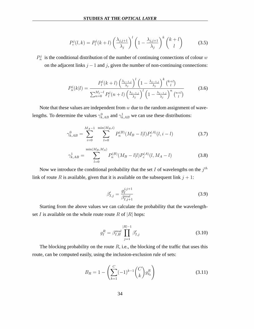
STUDIES AT THE OPTICAL LAYER
P jc (l, k) = P j
l (k + l)
(
λj,j+1
λj
)l(
1 −λj,j+1
λj
)k (k + l
l
)
(3.5)
P jn is the conditional distribution of the number of continuingconnections of colourw
on the adjacent linksj−1 andj, given the number of non-continuing connections:
P jn(k|l) =
P jl (k + l)
(
λj−1,j
λj
)l (
1 −λj−1,j
λj
)k(
k+l
l
)
∑Mj−l
n=0 P jl (n + l)
(
λj−1,j
λj
)l (
1 −λj−1,j
λj
)n(
n+l
l
)
(3.6)
Note that these values are independent fromw due to the random assignment of wave-
lengths. To determine the valuesγ0k,AB andγ1
k,AB we can use these distributions:
γ0k,AB =
MA−1∑
i=0
min(MB ,i)∑
l=0
P (B)n (MB − l|l)P (A)
c (l, i − l) (3.7)
γ1k,AB =
min(MB ,MA)∑
l=0
P (B)n (MB − l|l)P (A)
c (l,MA − l) (3.8)
Now we introduce the conditional probability that the setI of wavelengths on thejth
link of routeR is available, given that it is available on the subsequent link j + 1:
β′I,j =
gj,j+1I
βmulI,j+1
(3.9)
Starting from the above values we can calculate the probability that the wavelength-
setI is available on the whole route routeR of |R| hops:
gRI = βmul
I,H
|R|−1∏
j=1
β′I,j (3.10)
The blocking probability on the routeR, i.e., the blocking of the traffic that uses this
route, can be computed easily, using the inclusion-exclusion rule of sets:
BR = 1 −
(
C∑
k=1
(−1)k−1
(
C
k
)
gRIk
)
(3.11)
34

STUDIES AT THE OPTICAL LAYER
To get the total blocking probability of the network, we onlyneed to take the weighted
sum of theBR values. The weights are the normalised offered load values between each
pair of nodes, i.e., the values in the interest-matrix.
3.2.1.3 Feedback on the arrival characteristics
Let us show how load correlation effects can be considered inWDMM . Blocking on
routeR affects the offered load on each of its links. Thus, we can derive the intensity of
connection request arrival on linkj, givenm free optical channels on it:
αj(m) =∑
R:j∈R
λR(j,m)
min(m,C)∑
k=1
(−k)k−1
(
C
k
)
gR,jIk
(m))
(3.12)
whereλR(j,m) is the intensity of the traffic offered to routeR when there arem free
channels on linkj. For thePoissontraffic modelλR(j,m) does not depend onj andm.
For theBinomialandPascaltraffic types a more complex calculation is required.
The conditional probabilitygR,jI (m) means that the wavelength-setI is available on
routeR, given that there arem free channels on linkj. Using the same idea as in Equation
3.2 this probability can be calculated as:
gR,jI (m) =
gRI
βmulI,j
∑
min
�i, �Cj−m
Mj ��k=0 (−1)k
(
i
k
)(
Cj−Mjk
Cj−Mjk−m
)
(
Cj
Cj−m
) (3.13)
3.2.2 Complexity of the algorithm
Let us present now the complexity of theWDMM algorithm in terms of the characteris-
ing values of the network:
• the applied binomial coefficients can be obtained inO(C2M2) steps,
• the calculation of theβmulI,j values is in order ofO(JC3M),
• the auxiliary variablesPl, Pc andPn are computable in order ofO(JC2M2) +
O(HC) + O(HC),
35

STUDIES AT THE OPTICAL LAYER
• we needO(J2M2) + O(J2M) + O(JC2) steps to obtainγ(0), γ(1) andβ′.
The sum of these complexities gives the complexity of the whole calculation, that is
O(JC3M)+O(JC2M2)+O(J2M2). This complexity has to be considered in each step
of the iteration. The number of iteration steps depends strongly on the network load and
can not be easily estimated.
The computation is obviously more complex for the multifibercase than for the case
where only one fiber is allowed in each link. The model for thislatter case is presented
in [58] and has only the complexity in order ofO(JC2).
3.2.3 Numerical results
In order to observe the accuracy of theWDMM algorithm, we compared it with theMul-
tifiber Link-Load CorrelationmodelMLLC introduced in [52] and with simulations. We
present numerical results on the blocking probability of optical channel requests in func-
tion of the network load in different scenarios. The scenarios differ in topologies, fiber
capacities and traffic patterns. Another basis for model comparison is the computation
time, which refers the complexity of the algorithm.
Although our model accepts also traffic models that are better suited to WDM net-
works, in the studied scenarios the connection requests were assumed to arrive following
a Poisson process and with exponential holding time. Considering, that as nearly all pub-
lished solution,MLLC supports only thePoissontraffic model this is the only choice
that allows the model comparison.
In these illustrative studies the load is set to get blockingprobabilities in the range of
10−6 to 10−1. This range is too high for a traditional connection based service but can be
accepted in the IP over WDM scenario as we mentioned in Section2.3.2. On the figures
the network load is indicated in Erlangs. To accommodate theaccepted requests the
fixed shortest path routing is applied with the random wavelength assignment described
in Section 3.2.
We used the ASONCLES [38] tool for the simulation task. This simulator consid-
ers Automatic Switched Optical Networks and allows the investigation of different RWA
solutions. The simulations ran until the blocking probability as significant statistical vari-
able reached the confidence level0.99 with 0.01 accuracy around the point of estimate.
36

STUDIES AT THE OPTICAL LAYER
In the computations ofWDMM the iteration was stopped when the difference between
the blocking probability values got in two successive stepsdecreased under10−6.
3.2.3.1 Uniform ring topology
1e-06
1e-05
1e-04
1e-03
1e-02
1e-01
1e+00
25 30 35 40 45 50 55 60 65
Con
nect
ion
Blo
ckin
g P
roba
bilit
y
Network Load
SimulationWDMM
MLLC1e-06
1e-05
1e-04
1e-03
1e-02
1e-01
1e+00
25 30 35 40 45 50 55 60 65
Con
nect
ion
Blo
ckin
g P
roba
bilit
y
Network Load
SimulationWDMM
MLLC
Figure 3.2: Blocking probability in the uniform 13-node ring: for uniform traffic (left)
and non-uniform traffic (right)
The first results were obtained using a 13 node ring withCj = 24 optical channels
on each link. The number of wavelengthsC was set to 24. This network is a single fiber
uniform ring that is a very appropriate topology for the model validation because of the
high dependence of paths. The numerous common links in the paths imply also the high
dependence of the traffic coming from and going to different network nodes. We used a
uniform traffic pattern. Due to the uniformity this scenariosimplifies the study of basic
model properties.
The comparison of the theoretic modelsWDMM andMLLC with simulation results
can be seen on the left plot of Figure 3.2. One can see thatWDMM estimates accurately
the blocking probability, while the accuracy of theMLLC model is very good in the
light-load cases, but it overestimates the blocking rate incases of higher network load.
This behaviour may come from the fact, thatMLLC does not include any fixpoint search
mechanism.
In the next study case we setC to 6 and, concurrently,Mj to 4 for each link using the
same uniform ring topology. Here we applied a random generated non-uniform traffic
37

STUDIES AT THE OPTICAL LAYER
pattern. For this multifiber network we obtained the resultsshown on Figure 3.2 in the
right plot.
The large number of fibers causes that in the low-load area ourmodel underestimates
the simulated results of the blocking probability, while itis still accurate at high loads.
MLLC works similarly as in the above case.
Let us introduce now the comparison of the computation timesmeasured for the mod-
els that were used in the above study cases. All computationswere done on an Intel P4
system running at 2 GHz. The results given in seconds are presented in Table 3.1.
Table 3.1: Computation times for the uniform 13 node ring
Load WDMM MLLC WDMM MLLC
28.08 1 263 < 1 78
33.70 3 262 1 77
37.44 5 261 < 1 78
42.12 7 262 1 77
46.80 10 262 1 78
51.48 15 262 1 78
56.15 21 262 2 78
60.84 31 263 4 78
Uniform traffic,Mj = 1 Non-uniform traffic,Mj = 4
The computation times of the modelWDMM grows with the growth of the load. This
comes from the fact that using the same accuracy limit in the fixpoint search, the iteration
takes more steps to stop. It is easy to observe that the algorithm MLLC consumes much
more time than our method. The complexity of this method is not less thanO(HC5M3)
due to the use of recursive steps. This is considerably larger than the complexity of
WDMM presented in Section 3.2.2.
3.2.3.2 Non-uniform ring topology
The next set of results were obtained using a ring of 13 nodes with different Cj link
capacities. The total sum of the capacities in this network is the same as in the case of the
previously studied uniform ring, i.e.,24 ∗ 13 = 312 optical channels, the link capacities
38
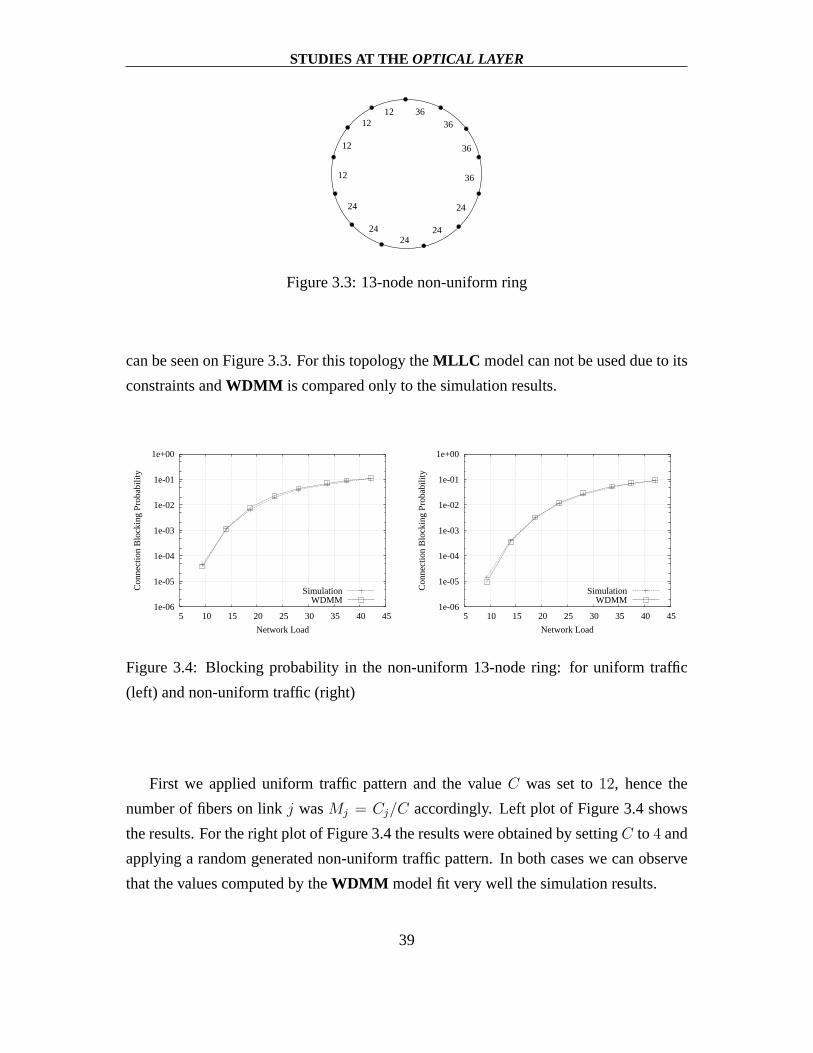
STUDIES AT THE OPTICAL LAYER
24
12
12
1212 36
36
36
36
24
2424
24
Figure 3.3: 13-node non-uniform ring
can be seen on Figure 3.3. For this topology theMLLC model can not be used due to its
constraints andWDMM is compared only to the simulation results.
1e-06
1e-05
1e-04
1e-03
1e-02
1e-01
1e+00
5 10 15 20 25 30 35 40 45
Con
nect
ion
Blo
ckin
g P
roba
bilit
y
Network Load
SimulationWDMM
1e-06
1e-05
1e-04
1e-03
1e-02
1e-01
1e+00
5 10 15 20 25 30 35 40 45
Con
nect
ion
Blo
ckin
g P
roba
bilit
y
Network Load
SimulationWDMM
Figure 3.4: Blocking probability in the non-uniform 13-nodering: for uniform traffic
(left) and non-uniform traffic (right)
First we applied uniform traffic pattern and the valueC was set to12, hence the
number of fibers on linkj wasMj = Cj/C accordingly. Left plot of Figure 3.4 shows
the results. For the right plot of Figure 3.4 the results wereobtained by settingC to 4 and
applying a random generated non-uniform traffic pattern. Inboth cases we can observe
that the values computed by theWDMM model fit very well the simulation results.
39

STUDIES AT THE OPTICAL LAYER
Berlin
Prague
London
Amsterdam
250, 96
Copenhagen
Milan
300, 128
500, 64
Paris
Brussels500, 96
660, 64Zurich
350, 64
Vienna Budapest
500, 160280, 128
220, 64
250, 32
280, 32
350, 32
280, 64500, 96
600, 96
600, 32
375, 96
500, 64
470, 96
Figure 3.5: Central-West European Network
3.2.3.3 CWEN topology
After the evaluation of the proposed model on regular topologies let us present results
using a meshed network. The hypothetic Central-West European network shown on Fig-
ure 3.5 consists of 11 nodes and 19 optical links. The numberson the links are the length
derived from the distance in kilometres and the capacity in wavelengths. Its design was
based on previous publications [60] and [61] that studied pan-European optical network
opportunities. The link capacities and the applied traffic pattern were determined consid-
ering a population-distance-based traffic relation matrix.
The number of wavelengthsC was set to32 in the first case and to16 in the second
case. The results are presented on Figure 3.6 left and right plot respectively. We can
observe the robust accuracy of theWDMM model in both cases.
3.3 Discussion
In this chapter we presented the results of the studies performed considering only the
optical layer. A theoretical model was introduced to capture the issue of the optical
request blocking probability computation.
Summarising our experiences, on the one hand, we have that the WDMM model
estimates well the blocking probability of optical connection request. This is due to its
40
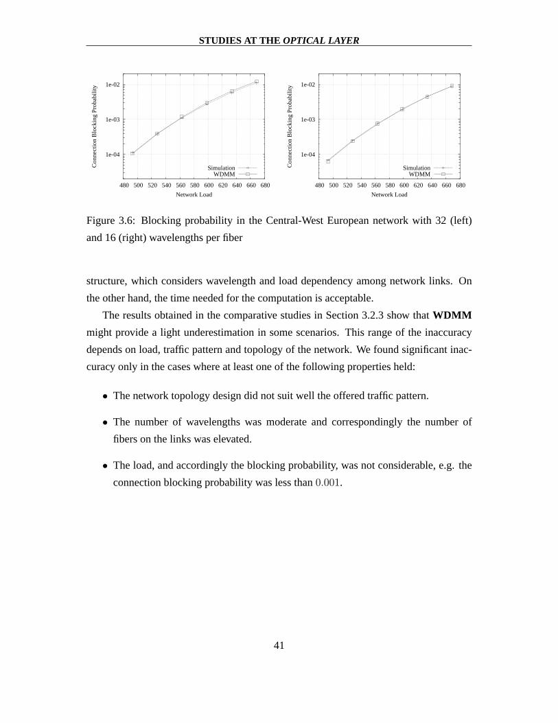
STUDIES AT THE OPTICAL LAYER
1e-04
1e-03
1e-02
480 500 520 540 560 580 600 620 640 660 680
Con
nect
ion
Blo
ckin
g P
roba
bilit
y
Network Load
SimulationWDMM
1e-04
1e-03
1e-02
480 500 520 540 560 580 600 620 640 660 680
Con
nect
ion
Blo
ckin
g P
roba
bilit
y
Network Load
SimulationWDMM
Figure 3.6: Blocking probability in the Central-West European network with 32 (left)
and 16 (right) wavelengths per fiber
structure, which considers wavelength and load dependencyamong network links. On
the other hand, the time needed for the computation is acceptable.
The results obtained in the comparative studies in Section 3.2.3 show thatWDMM
might provide a light underestimation in some scenarios. This range of the inaccuracy
depends on load, traffic pattern and topology of the network.We found significant inac-
curacy only in the cases where at least one of the following properties held:
• The network topology design did not suit well the offered traffic pattern.
• The number of wavelengths was moderate and correspondinglythe number of
fibers on the links was elevated.
• The load, and accordingly the blocking probability, was notconsiderable, e.g. the
connection blocking probability was less than0.001.
41

Chapter 4
Performance of thedata layer
4.1 Introduction
This chapter treats performance analysis in thedata layer, with a specific interest on
the IP routing solution. The aim of this work was on the one hand, to find efficient but
correct ways to assess network capabilities. On the other hand, the study of the existing
algorithms can help us to develop new ones providing higher performance.
Many works were presented in the last decade on IP networks performance analysis
and about the viable solutions. The emerging of the IntServ [14] and DiffServ [15] ar-
chitectures for the future Internet, together with the possibility of building backbone Au-
tonomous Systems based on Multiprotocol Label Switching (MPLS) [62] and the need
for provisioning Quality of Service (QoS) in the Internet spawned a burst of work con-
cerning new, QoS-based, dynamic routing algorithms suitable for implementation in IP
networks.
Some examples obtained from the research effort on QoS routing can be found in
[2, 20, 63, 64]. Besides the examination of the service quality aspect that is mostly
represented in our studies as the effective transport rate of flows and the prevalence of
starvation situation, also other points of view can be foundfor comparison of routing
performance. Researchers focused their attention upon other aspects of QoS routing too,
namely protocol overhead [2, 21] and implementation issues[63, 64].
Nearly all of the previous works assume flow based models representing the IP traffic
42
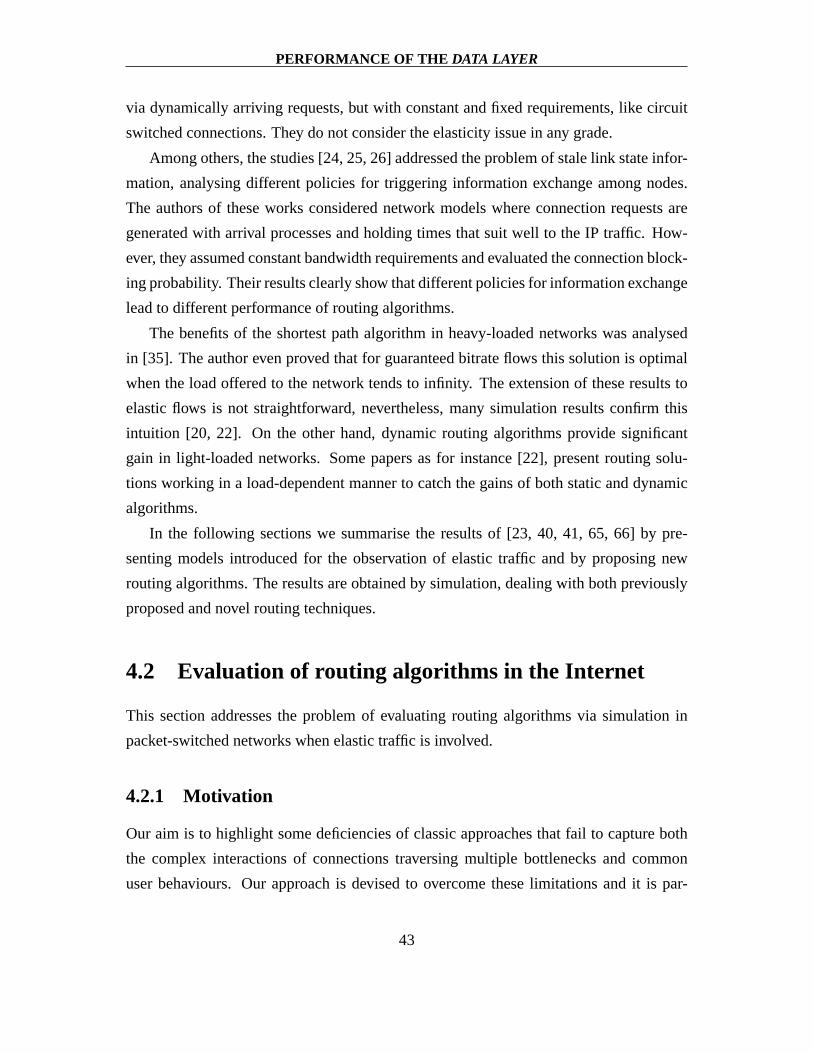
PERFORMANCE OF THE DATA LAYER
via dynamically arriving requests, but with constant and fixed requirements, like circuit
switched connections. They do not consider the elasticity issue in any grade.
Among others, the studies [24, 25, 26] addressed the problemof stale link state infor-
mation, analysing different policies for triggering information exchange among nodes.
The authors of these works considered network models where connection requests are
generated with arrival processes and holding times that suit well to the IP traffic. How-
ever, they assumed constant bandwidth requirements and evaluated the connection block-
ing probability. Their results clearly show that differentpolicies for information exchange
lead to different performance of routing algorithms.
The benefits of the shortest path algorithm in heavy-loaded networks was analysed
in [35]. The author even proved that for guaranteed bitrate flows this solution is optimal
when the load offered to the network tends to infinity. The extension of these results to
elastic flows is not straightforward, nevertheless, many simulation results confirm this
intuition [20, 22]. On the other hand, dynamic routing algorithms provide significant
gain in light-loaded networks. Some papers as for instance [22], present routing solu-
tions working in a load-dependent manner to catch the gains of both static and dynamic
algorithms.
In the following sections we summarise the results of [23, 40, 41, 65, 66] by pre-
senting models introduced for the observation of elastic traffic and by proposing new
routing algorithms. The results are obtained by simulation, dealing with both previously
proposed and novel routing techniques.
4.2 Evaluation of routing algorithms in the Internet
This section addresses the problem of evaluating routing algorithms via simulation in
packet-switched networks when elastic traffic is involved.
4.2.1 Motivation
Our aim is to highlight some deficiencies of classic approaches that fail to capture both
the complex interactions of connections traversing multiple bottlenecks and common
user behaviours. Our approach is devised to overcome these limitations and it is par-
43
PERFORMANCE OF THE DATA LAYER
ticularly suited for the evaluation of routing algorithms in presence of best-effort traffic.
The simulation results presented offer a deeper insight into well-known routing algo-
rithms. Through this analysis it is clear that quantitativeand also qualitative behaviours
of dynamic routing algorithms based on traffic measurementsmay be fairly different de-
pending on the nature of the traffic loading the network, as well as depending on its
interactions with the network parameters and behaviour.
As one could see in Section 2.6.4 purely theoretical tools can have hard limits if more
realistic traffic and more complex algorithms need to be modelled. Most of the network
functions can be efficiently implemented in a simulator, although not always in a very
easy way. A big advantage is the robustness in realising new models.
The drawback of simulation can be that no general and straightforward statements
can be done based on the obtained results. While theory can provide clear and proved
answers on several questions regarding the performance of network solutions, simulation
results can always depend on the investigated scenario. Forinstance, analysing the per-
formance of QoS routing algorithms to get general conclusions several different topolo-
gies and traffic loads need to be simulated. Since networks need a routing strategy that
is first of all robust to changing traffic patterns and loads, achieving high performance in
some selected scenarios, while performing poorly in othersmay be worse than using a
routing strategy whose performance is possibly not the bestfor any traffic pattern, but is
predictable and ensures reasonable performance under any circumstance.
4.2.2 Basic assumptions
Performance evaluation in IP networks can be performed withanalysis on packet-level.
Note that this solution results in a very complex model, whose simulation is generally
too expensive to obtain reasonable results for any realistic network. Instead, we use
flow-level traffic models in the simulations. Going more in details on thedata layerin the
general network vision presented in Section 2.1 we use the following general assumptions
in the rest of this section.
• The network nodes have unlimited capacity in both switchingand throughput. A
node of thedata layeris able to switch any flow from any incoming link to any
outgoing one if the links can accept the traffic.
44
PERFORMANCE OF THE DATA LAYER
• Buffering is not modelled, assuming that the packet loss and delay problem is
implicitly solved with the elastic model of the flows.
• We do not consider the details of the switching mechanism andits timing.
• Network users are attached to the nodes.
• Generators connected to network users pump the traffic in a flow oriented manner
according to the total network loadρ and the traffic pattern.
• In any instant, for any link, the sum of instantaneous data rate of flows carried by
the link can not be greater then the link capacity.
• Flow management functions are present in the network and we assume a control
plane that fully connects them and carries the needed OAM-type information. This
allows us to model network traffic as flows, even if from network management
point of view the endpoints are not connection oriented.
• Once a path is assigned to a flow, the data transport is performed using this path
until the user finishes to carry traffic.
• The instantaneous data transport rate of the flowf is identical on each link of the
assigned route and is stated asBf .
• Flows may have a maximum data rateBM derived from the access link or applica-
tion output constraints.
Connections originating from users with service guaranteesreceive the resources con-
tracted in the SLA. However, analysing thedata layerthat models the IP network, we
are rather interested in the performance of the best-efforttraffic. For this type of traffic
the network does not guarantee any value of the data rate and these flows share link re-
sources adaptively. We assume max-min-fair-sharing described in [35] and analysed in
[67], since no priority among the flows is considered. This leads to a behaviour where
elasticity is a dominant phenomenon.
The elastic approach can be easily validated if we consider that the Internet traffic
is mostly carried over TCP. Adaptivity is embedded in the congestion control algorithm
45
PERFORMANCE OF THE DATA LAYER
of the TCP protocol which is a closed-loop protocol with implicit feedback from the
network. The modelling technique used in our studies does not address the details of TCP
protocol, but tries to partially capture its self-controlling behaviour from the consumed
bandwidth point of view. For instance, the reaction to network congestion spread the
connection over time and result in congestion periods that last longer than what can be
estimated with a model devoid of any feedback feature. The aim of TCP congestion
control is sharing network resources following max-min fairness, and this is exactly the
adaptivitycriterion we use. Indeed, some authors in [68] have suggested that feedback
phenomena, making the load offered to the network dependentfrom the network status
and parameters, might be responsible for the LRD (long range dependent) behaviour of
Internet traffic1.
In addition, the model considers the concept offlow starvation, another typical feature
of the Internet, specially related to Web browsing. It is well known that caused by the
lack of admission control the number of connections using the network at the same time
is virtually unlimited. As a result, TCP packets might be lostdue to congestion, leading
to frequent retransmissions and consequently longer transfer completion time; similarly,
UDP packets belonging to a streaming multimedia connectioncould be dropped, leading
to unacceptably poor playback quality. In either case, users will abort the connection and
may retry to download the data later.
This behaviour can seriously affect the network performance, since the network does
some effort to transfer information which might turn out to be useless. Furthermore,
resources devoted to aborted connections appear to be unnecessarily taken away from
other connections. To emulate the sudden closure of starvedconnections, we define a
connection asstarvedwhen the amount of bandwidth resources it receives falls below a
given threshold.
4.2.3 Modelling elastic traffic connections
We defined two modelling paradigms of data transfer in [41], they are used in the flow-
level analysis of different user traffic. After their description we give a more detailed
insight into the issue of modelling the starvation effect.
1The study of this issue is out of our scope.
46

PERFORMANCE OF THE DATA LAYER
4.2.3.1 Time-Based model
The most common traffic model used in high-level communication networks simulation
is Time-Based (TB). In this model, connections are described by their duration (hold-
ing time), and by their bandwidth requirements. For example, in telephone networks,
connections require a CBR (Constant Bit Rate) service; this pieceof information, inte-
grated by the connection interarrival time and the requiredbandwidth, is sufficient both
to determine the traffic intensity produced by the connection generator and to completely
characterise the connection from the network point of view.The network can allocate
enough resources to guarantee the required QoS. A similar approach is valid for variable
rate connections. Any given CAC (Connection Admission Control) scheme can be im-
plemented in simulation to control the network load and satisfy the QoS requirements of
connections.
The effectiveness of this model is questionable if best-effort, data-based connections
are considered. Defining a priori adurationfor such a traffic is virtually impossible, since
these connections are data-centric, considering the information to be exchanged the most
important part of the communication. Typically using a besteffort service, these data-
centric connections adapt their sending rates to the current network congestion, which
cannot be known a priori. Thus a new model must be used to describe this kind of traffic.
In a Time-Based model, we can still derive some kind of connection duration, but
it can usually be obtained making hypothesis on the bandwidth the connection could
obtain in the communication. SinceTB is not able to model veritably the whole process
of data transfer, indeed, a distortion of the network throughput can affect the analysis.
While in the case of CBR traffic the total amount of traffic offeredto the network could
be precalculated using the predetermined holding time, in the case of elastic traffic no
obvious derivation can be done. If the actually achieved perflow throughput, i.e, the
bandwidth that is currently assigned to the flow, decreases,the instantaneous offered
traffic decreases too. The flow request arrival rate remains invariable but the data amount
transferred by the connection gets smaller.
47

PERFORMANCE OF THE DATA LAYER
4.2.3.2 Data-Based model
The (TB) model fails when we try to apply it to the typical data exchange in Internet,
such as data downloads from the Web or FTP transfers. In all these situations the objects
of communication are files and the communication ends when the last bit of the file has
been acknowledged. Even if we declare a maximum communication rateBM that em-
ulates the limitations introduced by the application, the transport protocol, or the access
network, it is of little help, because it only sets the lower bound for the connection du-
ration. However, considering thestarvation effectan upper bound can be also calculated
for this value.
Indeed, the actual time required to successfully end the data transfer depends on many
factors, and mainly from the varying available bandwidth while the connection is active.
Thus we introduce the Data-Based (DB) traffic model, where the connection lasts until all
the data amountSD associated to the flow is transmitted. This way no distortionaffects
the offered traffic. Figure 4.1 illustrates the main difference toTB.
assigned bandwidth
data difference
t0
assigned bandwidth
M
M
B
B
TB
DB
time difference
Figure 4.1: Traffic modelsTBandDB
Since in the flow-level simulation approach the packet transmission is not simulated,
we need to estimate dynamically the time the transmission ends. Since connections with
elastic bandwidth requirements generally use all their share of available bandwidth (up to
their maximum transmission rate) duration can be determined only by monitoringsemi-
48

PERFORMANCE OF THE DATA LAYER
continuouslythe instantaneous bandwidth allocated to the connection. In a simplified
model the values of assigned bandwidth can change only at time-points of the arrival
or departure of connections with any characteristic. We canobtain them by running a
max-min fair-share algorithm that requires a full recalculation of the bit rate of all con-
nections currently routed in the network every time a flow is opened or closed. Actually
this solution provides an upper bound to the performance, since the max-min fair-share
represents an ideal working situation for any congestion control protocol that aims at
equally dividing resources among the elastic flows, as the TCPprotocol tries to achieve.
4.2.3.3 Modelling the starvation
To model the starvation effect, i.e., users that abort the data transfer due to poor per-
formance, we introduce astarvation thresholdbm that will be used to identify starved
connections and realises an implicit definition of the minimum acceptable bandwidth for
the flow. If for any flowf the current per-flow bit rate estimate on a bottleneck linkBf
drops belowbm, then the connection with the longest remaining time of data-transfer is
picked and terminated. The choice of the connection that would hold on for the longest
time models the behaviour of a general user that aborts the most delaying data transfer.
The only exception for the choice is a currently started connection whose termination,
emulating this way an implicita priori CAC, is not allowed.
A starvation situation can evolve not only after the openingof a new flow. In certain
scenarios the departure of a flow causes the starvation of other flows.
This mechanism allows us to define thestarvation probabilityps as the ratio between
connections that are prematurely terminated and the total number of connections that en-
tered the network. The information about service quality that this probability value gives
us, is similar to the blocking probability value in networkswith connection admission
control function and has to be considered in the performanceevaluation.
4.2.4 Formulation of the routing algorithms
The flow-based approach of the introduced data and traffic models reflects the concept
of flow identification possibility in the transport servicesthat support QoS, e.g. IntServ,
DiffServ or MPLS. According to this idea we make an assumption about the routes cho-
49

PERFORMANCE OF THE DATA LAYER
sen to carry best effort traffic. A transport path is assignedto a flow request arriving
in nodes, choosing it with the routing algorithm once and for all, i.e. the same path is
used for all the flow-data. This way we exclude the option of using multiple paths, as for
instance in-node flow control techniques of packet-based network models that allow to
assign different paths to the fragments of the transported data.
To understand the workout of the used routing algorithms we introduce a general
notation and formulation: a generic network is referred as adirected graphG = (V , E),
whereV is the set of vertices (accord to network nodes), andE is the set of edges (accord
to network links) that can be weighted by different metricsω.
A pathπ(vs, vd) of lengthn = ||π(vs, vd)|| hops is defined as a sequence ofn distinct
edgesei joining vs andvd, wherevs, vd ∈ V, ei ∈ E , π(vs, vd) = {e1, e2, ..., en}.
A setPG is defined as the set of all paths existing between any two distinct vertices
of G, i.e.,PG = {π(vs, vd)|vs, vd ∈ V, vs 6= vd}. This set can be divided into disjoint
subsets corresponding to the starting and ending node of network route: PG(s, d) =
{π(vs, vd)}.
A weight wωi can be assigned to each linkei using any metricω that combines topo-
logical, physical or traffic-related characteristics of that link. A costcγ(π) is assigned to
each pathπ using a combination of the weights of its links whereγ identifies the combi-
nation method. Following this, an order relation≺ in each subsetPG(s, d) is established
among the paths according to their costscγ, and we can refer to a pathπi as “lighter than”
πj if πi ≺ πj holds. If neitherπi ≺ πj norπj ≺ πi hold,πi andπj areequicostpaths by
the given cost functionγ.
If we do not indicate it differently, path costs are real values and the applied ordering
relation is the ascending ordering among real values, i.e.,πi is lighter thanπj according
to the cost metricγ if and only if cγ(πi) < cγ(πj).
In routing decisions the combined use of different costs areallowed. The simplest
combination is the concatenation, formulated as:cγ1 ⊕ cγ2. This combined solution im-
plies that after the ordering bycγ1 theequicostpaths will be reordered bycγ2. Conditional
use of different cost functions and, as one can see in latter sections, reduction of the sub-
setsPG(s, d) can be applied too.
50
PERFORMANCE OF THE DATA LAYER
Commonly used weight metrics of edges are the following.
H assigns the same constant weight to each link,wHi = a|ei ∈ E . As most common
value,a can be set to1 representing onehop, in the following we will use this
value.
L assigns constant weight for linkei, representing itslength. wLi = li|ei ∈ E .
RES assigns as weight the value ofresidualbandwidth measured on the link, i.e., the
bandwidth available for the best effort traffic.wRESi = BRES(ei) = BTOT (ei) −
BGAR(ei)|ei ∈ E , whereBTOT (ei) is the total bandwidth capacity of linkei and
BGAR(ei) is the bandwidth currently assigned to traffic with bandwidth guarantees.
ABW weight metric is based on the bandwidth value that isavailablefor a new best ef-
fort connection on the link, assuming fair sharing of the residual bandwidth among
the best effort connections.wABWi = BRES(ei)
NBEi +1
|ei ∈ E , whereNBEi is the current
number of best effort connections, i.e., identified elasticflows on linkei.
The weight assigning functionsH andL are time independent, whileRES andABW
depend on the current network state. Routing algorithms thatconsider information on the
network state are known in the literature asdynamicor adaptiveschemes.
Let us define a special cost function that is not derived from edge weights:cRND(π)
is a randomly chosen value between0 and1. RND costs can be assigned either a priori
or at the moment of cost evaluation, this two versions are referred asRNDA andRNDC
respectively. We impose that there are noequicostpaths in the subsetsPG(s, d) through
the costsRNDA andRNDC.
Now we give a brief description of some known routing algorithms. A set of them will
be used in the analysis assessing the difference between thetraditional traffic modelling
technique based on holding time (Time-Based), and the novel one based on the amount
of generated data (Data-Based). Later on these algorithms will be used in the analysis
of new routing algorithms as comparison basis. Unless otherwise stated, the choice is
always the “lightest” path with the given ordering system.
• Fixed-Shortest-Path(FSP): for each source-destination pair, the algorithm deter-
mines the path with the minimum hop count and routes flows along that path. If
51
PERFORMANCE OF THE DATA LAYER
two or moreshortestpaths exist, the algorithm chooses one at random2, that is used
during the whole data transmission period of the flow. This isthe routing algorithm
commonly used in the Internet (e.g., OSPF). Its formal definition is a concatenation
of orderings by the cost functionscH(π) =∑
ei∈π wHi andcRNDA(π), or in shorter
form: cFSP = cH ⊕ cRNDA.
• Widest-Shortest(WS): for each source-destination pair, the algorithm determines
the path with the minimum hop count. If more than one such pathexists, it breaks
the tie by choosing the one with the largest available bandwidth for the new con-
nection. The formal definition of the ordering:cWS = cH ⊕ cABW ⊕ cRNDA, with
cABW (π) =1
minei∈π wABWi
(4.1)
The implemented scheme operates as in the original proposalin [69], except in the
case of multi-class scenarios. We use the share of bandwidthavailable to the new
flow taking into account that resources used by guaranteed traffic are no longer
available to the elastic best-effort traffic. The original proposal considers in the
link weight calculation the whole physical link capacityBTOT (ei).
• Minimum-Distance(MD): as proposed in [20, 67], for each source-destination pair
the pathπ is chosen which minimises a quantity that consider both the number of
hops in path and the available bandwidth on its links, and canbe described as a
special kind of distance between the end nodes. Formally we order by: cMD =
cRS ⊕ cH ⊕ cRNDA, where
cRS(π) =∑
ei∈π
1
wABWi
(4.2)
Note that the authors in [67] state that the algorithm is to beimplemented over
networks employing max-min fair-share-based congestion control. In our case, we
assume that the network can determine what the current max-min fair-share situa-
tion is at the time when the routing algorithm is executed, though this hypothesis
may be optimistic.
2It is possible to optimise theRNDA order, for example using load-balancing criteria.
52
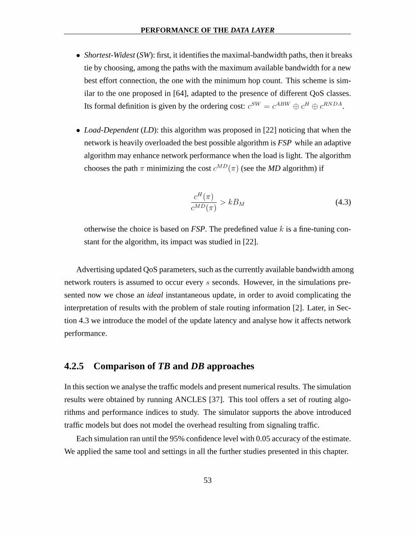
PERFORMANCE OF THE DATA LAYER
• Shortest-Widest(SW): first, it identifies the maximal-bandwidth paths, then it breaks
tie by choosing, among the paths with the maximum available bandwidth for a new
best effort connection, the one with the minimum hop count. This scheme is sim-
ilar to the one proposed in [64], adapted to the presence of different QoS classes.
Its formal definition is given by the ordering cost:cSW = cABW ⊕ cH ⊕ cRNDA.
• Load-Dependent(LD): this algorithm was proposed in [22] noticing that when the
network is heavily overloaded the best possible algorithm isFSP while an adaptive
algorithm may enhance network performance when the load is light. The algorithm
chooses the pathπ minimizing the costcMD(π) (see theMD algorithm) if
cH(π)
cMD(π)> kBM (4.3)
otherwise the choice is based onFSP. The predefined valuek is a fine-tuning con-
stant for the algorithm, its impact was studied in [22].
Advertising updated QoS parameters, such as the currently available bandwidth among
network routers is assumed to occur everys seconds. However, in the simulations pre-
sented now we chose anideal instantaneous update, in order to avoid complicating the
interpretation of results with the problem of stale routinginformation [2]. Later, in Sec-
tion 4.3 we introduce the model of the update latency and analyse how it affects network
performance.
4.2.5 Comparison ofTB and DB approaches
In this section we analyse the traffic models and present numerical results. The simulation
results were obtained by running ANCLES [37]. This tool offers a set of routing algo-
rithms and performance indices to study. The simulator supports the above introduced
traffic models but does not model the overhead resulting fromsignaling traffic.
Each simulation ran until the 95% confidence level with 0.05 accuracy of the estimate.
We applied the same tool and settings in all the further studies presented in this chapter.
53

PERFORMANCE OF THE DATA LAYER
4.2.5.1 Simulated network and scenario
In order to decouple performance comparisons from a particular topology, a randomly
generated network topology was selected. The generating tool was the software GT-
ITM, introduced in [70]. The resulting topology comprises 32 nodes with an average
connectivity degree of 4 and uniform link capacityBTOT (ei) = 10 Mbps for each linkei.
The offered traffic is generated by best-effort source generators (one per node), trying to
set up connections with a maximum bandwidthBM of 1 Mbps. Each connection requires
a bulk data transfer whose sizeSD is randomly chosen from an exponential distribution
with average 500 kbytes. A uniform traffic pattern is simulated, i.e., when a new flow re-
quest is generated, the source-destination pair is randomly chosen according to a uniform
distribution.
This is hardly a scenario favouring QoS routing, and we choseit exactly for this
reason: non-uniform, “hot-spot” traffic scenarios may favour specific QoS routing algo-
rithms, altering the perception of the relative merits of each algorithm. As a consequence
of this choice, the gains we can expect from QoS routing are limited compared toFSP.
The load offered to the network is expressed in Mbps. The meannumber of flows
that arrive in the network each second can be easily computedknowing the mean bulk
data sizeSD. Dividing it by 32 we get the requests per second value per generator. For
instance, an offered load of 320 Mbps corresponds to a nominal network flow request
arrival rate of(320Mbps)/(8 ·500 kbit) = 80 flow per seconds, hence each single gener-
ator offers80/32 = 2.5 request per second load, i.e., averagely 10 flow requests in every
4 seconds. The actual throughput carried by the network depends on the efficiency of the
applied routing algorithm.
The holding timeHt of Time-Based connections is computed based on the informa-
tion amount and the maximum required bandwidth:
Ht = SD/BM (4.4)
If instead we use the DB model, this calculation gives a lowerbound of the real
holding time. The elastic manner of their assigned bandwidth can affect the time needed
to transfer the currently remaining traffic in each moment.
As performance indices, we report the starvation probability ps and the average band-
width or throughput per connectionT , defined as the mean value of bandwidth that con-
54
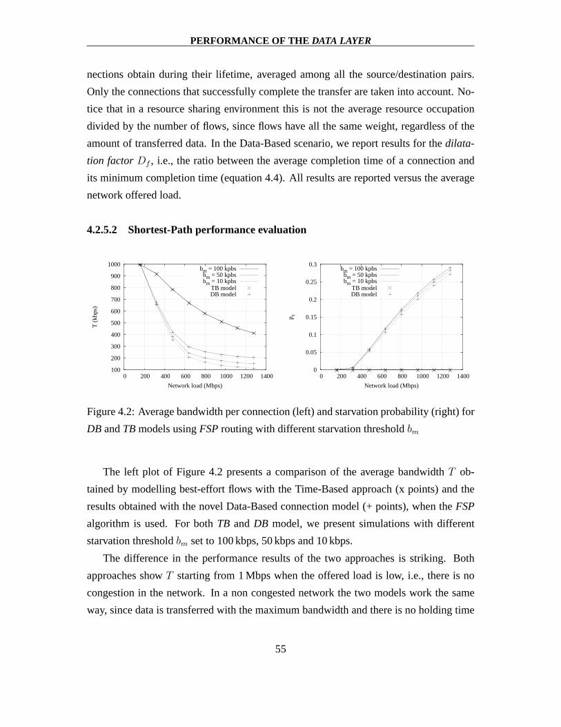
PERFORMANCE OF THE DATA LAYER
nections obtain during their lifetime, averaged among all the source/destination pairs.
Only the connections that successfully complete the transfer are taken into account. No-
tice that in a resource sharing environment this is not the average resource occupation
divided by the number of flows, since flows have all the same weight, regardless of the
amount of transferred data. In the Data-Based scenario, we report results for thedilata-
tion factorDf , i.e., the ratio between the average completion time of a connection and
its minimum completion time (equation 4.4). All results arereported versus the average
network offered load.
4.2.5.2 Shortest-Path performance evaluation
100
200
300
400
500
600
700
800
900
1000
0 200 400 600 800 1000 1200 1400
T (
kbps
)
Network load (Mbps)
bm = 100 kpbsbm = 50 kpbsbm = 10 kpbs
TB modelDB model
0
0.05
0.1
0.15
0.2
0.25
0.3
0 200 400 600 800 1000 1200 1400
p s
Network load (Mbps)
bm = 100 kpbsbm = 50 kpbsbm = 10 kpbs
TB modelDB model
Figure 4.2: Average bandwidth per connection (left) and starvation probability (right) for
DB andTBmodels usingFSProuting with different starvation thresholdbm
The left plot of Figure 4.2 presents a comparison of the average bandwidthT ob-
tained by modelling best-effort flows with the Time-Based approach (x points) and the
results obtained with the novel Data-Based connection model(+ points), when theFSP
algorithm is used. For bothTB andDB model, we present simulations with different
starvation thresholdbm set to 100 kbps, 50 kbps and 10 kbps.
The difference in the performance results of the two approaches is striking. Both
approaches showT starting from 1 Mbps when the offered load is low, i.e., thereis no
congestion in the network. In a non congested network the twomodels work the same
way, since data is transferred with the maximum bandwidth and there is no holding time
55

PERFORMANCE OF THE DATA LAYER
dilatation in the case of theDB model.
On the other hand, the two models drastically differ when theoffered load starts
increasing. Indeed, the Data-Based model shows a decrease inT and the performance
tends to the thresholdbm that acts as a lower bound on this performance index. On the
contrary, the Time-Based approach shows a smoother decreaseof the average bandwidth,
and independency on the thresholdbm.
When the available bandwidth goes below the starvation threshold, connections begin
to be aborted. We presented simulation results on the starvation probability inDB and
TB models on the right plot in Figure 4.2. In the case of the Time-Based approachps
is always zero, explaining the independence ofT on bm. Although simulation were
performed with differentbm thresholds, in the case of the Data-Based approach we do
not measure a significant variation in the starvation probability. This behaviour can be
interpreted as a much lower impact of the threshold on the starvation of connections than
on the assigned bandwidthT . In other words, major part of the connections that suffer
the starvation effect with thresholdbm, would be interrupted also using a lower threshold
b′m. Since flows with thresholdb′m are less sensitive on congested situations, the mean
lifetime of the starved connections is not smaller than of those using thresholdbm. Thus,
using lower starvation thresholds implies that a not completed flow wastes the network
resources for longer time, while the ratio of the starved flows does not change too much.
To explain the not negligible differences in the performance measures, on the one
hand the experimented characteristics ofT andps are due to two factors derived from the
model structure:
• In the Data-Based approach, when congestion arises in the network, connections
are throttled. This causes a stretching-out of the durationof the connections that
require more time to be successfully ended, thus spreading congestion over time.
A sort of avalanche effect occurs, as the number of connections increases on a
bottleneck link, reducing the available bandwidth for eachof them. In other words,
there are always more connections that share network resources when using theDB
model, with respect to theTBmodel.
• On the contrary, in the Time-Based model, the congestion doesnot spread over
time, since the holding time of the flows is determineda priori and it is not affected
56

PERFORMANCE OF THE DATA LAYER
by the congestion. Thus, no avalanche effect on congestion is possible, since the
average number of connections is independent of congestion.
On the other hand, we experienced that the data amount transmitted with finalised
flows, is only a part of the total offered load. Whenbm was 100 kbps the ratio of finalised
and offered traffic decreased in a roughly linear way down to 40% with the load increas-
ing up to 1260 Mbps. Although this degradation effect of network throughput at high
loads is similar for both theTB andDB models, the causes are different:
• Using theDB approach we get not finalised traffic due to the starved flows.
• In the case ofTBmodel there is no starvation. Here we have to refer the throughput
distortion mentioned in Section 4.2.3.1: the same arrival rate as inDB can reflect
in lower amount of data to be transferred inTB.
4.2.5.3 Comparison of routing algorithms
In this subsection, we present a set of results that aims at showing the difference in per-
formance obtained with the two traffic models when QoS routing algorithms are adopted
in the network. Generally, when comparing routing algorithm performance, we are inter-
ested in the relative merit with respect to well-established algorithms, such as the Fixed-
Shortest-Path (FSP). Thus, as performance index, we can select the relative gain of the
average throughputη obtained using a QoS-aware routing algorithm with respect to FSP
i.e.,η(r) = T (r)/T (FSP), whereT (r) is the average throughputT measured when using
ther routing algorithm.
The left plot of Figure 4.3 presents the relative throughputgain obtained with the
Time-Based model, while the right one shows that with the Data-Based model. Results
are for a scenario where the thresholdbm is 100 kbps.
Throughput results are comparable to previous studies (e.g. [20, 22]). The adaptive
MD andWSalgorithms outperformFSProuting on networks with relatively low load, as
they manage to exploit the spare bandwidth that is present onlightly loaded links. In-
stead, they provide a worse performance when the network becomes overloaded, because
of the waste of bandwidth that occurs when longer paths are selected. This behaviour of
adaptive routing algorithms can be observed in nearly all cases that we examined.
57
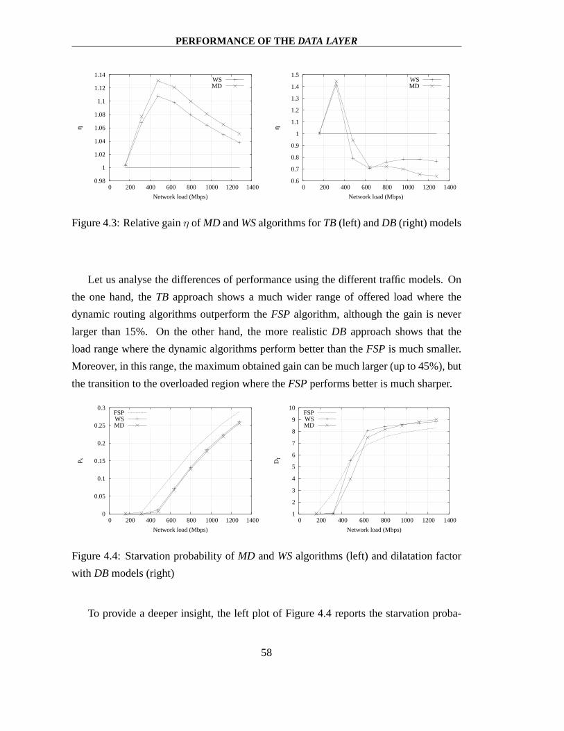
PERFORMANCE OF THE DATA LAYER
0.98
1
1.02
1.04
1.06
1.08
1.1
1.12
1.14
0 200 400 600 800 1000 1200 1400
η
Network load (Mbps)
WSMD
0.6
0.7
0.8
0.9
1
1.1
1.2
1.3
1.4
1.5
0 200 400 600 800 1000 1200 1400
η
Network load (Mbps)
WSMD
Figure 4.3: Relative gainη of MD andWSalgorithms forTB (left) andDB (right) models
Let us analyse the differences of performance using the different traffic models. On
the one hand, theTB approach shows a much wider range of offered load where the
dynamic routing algorithms outperform theFSPalgorithm, although the gain is never
larger than 15%. On the other hand, the more realisticDB approach shows that the
load range where the dynamic algorithms perform better thantheFSP is much smaller.
Moreover, in this range, the maximum obtained gain can be much larger (up to 45%), but
the transition to the overloaded region where theFSPperforms better is much sharper.
0
0.05
0.1
0.15
0.2
0.25
0.3
0 200 400 600 800 1000 1200 1400
p s
Network load (Mbps)
FSPWSMD
1
2
3
4
5
6
7
8
9
10
0 200 400 600 800 1000 1200 1400
Df
Network load (Mbps)
FSPWSMD
Figure 4.4: Starvation probability ofMD andWSalgorithms (left) and dilatation factor
with DB models (right)
To provide a deeper insight, the left plot of Figure 4.4 reports the starvation proba-
58
PERFORMANCE OF THE DATA LAYER
bility. Only the values achieved with theDB model are presented, since forTB all the
values were zeros as in case ofFSP. They suggest that the waste of bandwidth caused
by the starved connections can be rather high, as the starvation probability grows to large
values as soon as the offered load is larger than 450 Mbps.
Correlating Figures 4.3 and 4.4, it seems clear that the peak throughput gain ofMD
andWSwith respect toFSPis coincident with the network load where connections begin
to starve ifFSP is used, but still receive a satisfactory service ifMD or WSare used.
Even for higher load regions we find that the starvation probability is smaller when the
WSor MD algorithms is used. This suggests that the network bears a larger number of
simultaneous connections, each one obtaining a smaller throughput, but still higher than
its starvation limit.
The average dilatation factor for the different routing algorithms is plotted on the
right plot of Figure 4.4, obviously, only for theDB model. It can be noted that theWS
algorithm degrades its performance very quickly as soon as the offered load is higher than
about 400 Mbps, while theMD algorithm performs better than theFSPalgorithm up to
600 Mbps. As one could expect, the curves of this plot are correlated with the the values
of average assigned bandwidth that are not plotted explicitly. Even if the relation of
averages can be complicated, it is easy to see that the less isthe assigned bandwidth, the
larger is the stretch-out of connection holding time. According to the starvation threshold
of the scenario, the maximal dilatation can be calculated asBM/bm = 10, which is an
asymptote in the right hand plot of Figure 4.4.
The elastic traffic model, together with the run-time starvation detection, shows that
the evaluation of routing strategies based on inadequate (or too simplistic) models, such
as the Time-Based one, is prone to gross approximations and even mistakes. Thus in all
further studies we used the more realisticDB model.
4.3 Networks with stale link state information
As referred before, adaptive, dynamic routing schemes outperform FSP in situations
where network load is not too heavy. On the other hand, benefits of QoS routing are
59

PERFORMANCE OF THE DATA LAYER
often questioned, mainly on the basis of the additional costs3 and the risk that stale infor-
mation about the network status may lead to wrong routing decisions.
In this section we introduce a model that includes a timeout-triggered protocol func-
tion of link state information exchange. We analyse the impact of out-of-date information
with different timeout values on several QoS routing algorithms.
4.3.1 Information distribution
Any distributed routing algorithm requires the exchange ofinformation among nodes
in order to compute the available routes and their current costs. The advantage of QoS
routing is maximal when the routing algorithm exploits information on current utilisation
of resources. This information, however, is prone to error measurements, and, most of all,
it quickly becomes outdated. Indeed, out-of-date load information can even lead to wrong
routing decisions that can cause an avalanche effect forcing other route selections to
choose the wrong paths. New routing algorithms are often proposed without considering
the key issue of robustness to non optimal working conditions.
The amount of the exchanged information, together with the impossibility of dis-
tributing load information in real-time, may eventually counterbalance the advantages of
QoS routing in favour of the simple, traditional Fixed Shortest Path routing.FSPwas
shown to guarantee a good network utilisation in heavily–loaded networks with uniform
traffic pattern [67].
Several studies [2, 25, 40] addressed the problem of unreliable link state information,
analysing different policies for triggering information exchange among nodes. These
works clearly show that different policies for informationexchange lead to different per-
formance of routing algorithms.
We used the above introduced traffic modelling technique andevaluation methods to
compare different QoS routing algorithms with stale information. The main performance
measures for elastic traffic are the average throughputT obtained during the flow life
and the probability of starvationps. The aim of a QoS routing algorithm in this case
is finding routes that maximise the average throughput that best effort flows experience
while minimising the starvation.
3both in term of computing complexity and increased signaling
60
PERFORMANCE OF THE DATA LAYER
This section contains studies on the sensitivity of different routing algorithms to in-
accurate link state information. This is mainly a consequence of the impossibility of
distributing information in real-time as mentioned above.Other phenomena, like inac-
curate link measures, may also influence the results, but aregenerally less critical. The
inaccuracy comes from two separate effects. On the one hand,it is difficult to measure
the current bandwidthavailablefor elastic traffic. On the other hand, the number of best
effort flowsNBE currently active on a link can be only estimated, since this type of traf-
fic is packet based in reality. The measurements made by the router can consider only a
window of finite number of packets and there is no guarantee that this window contains
packets from each flow which currently uses the link. Since the number of connections
is an indispensable factor during the calculation of theestimatedavailable bandwidth
for a new connection, the inaccuracy influences the decisionof dynamic QoS routing
algorithms, e.g. those introduced in Section 4.2.4.
4.3.2 Model and problem formulation
We consider a Timer Based Trigger information update protocol [2], disregarding im-
plementation details about the protocol and focusing on thedegradation of performance
induced by large update timestu. While it has been shown that other update policies can
outperform the time-driven policy, in stationary traffic conditions (as in the simulations)
all threshold-based policies can be described in terms of time-driven ones, since no sud-
den change in the traffic triggers an information update before the timeout expiration. In
our model the triggers of network links are not synchronisedamong themselves and in a
more detailed model differenttu values could be considered for the links.
The inaccuracy in the number of connections on a link is modelled by a multiplication
with a random variable with uniform distribution over the(1 − fina, 1 + fina) interval,
wherefina is a tuneableinaccuracy factor. Since this inaccuracy is strictly connected to
the burstiness of the best effort traffic entering the network as well as to the measuring
interval, the factor has to be set to a reasonable value that will be than valid for each link
of the network.
We need a rather simple extension to the notation introducedin Section 4.2.4 to in-
clude the update protocol in the model. Two of the weighting metrics are touched by the
61

PERFORMANCE OF THE DATA LAYER
non–continuous update of link state information:
RES(tu) is the version of metricRES, but theBRES(ei) value of the residual bandwidth
on link ei is not updated at each traffic change. For each link a series ofsamples is
available, captured by asynchronous evaluation in eachtu timeunits.
ABW (tu, fina) weights vary in two main points from the simpleABW weights. First,
the BRES(ei) values of the bandwidth on linkei that remains available for the
best effort connections is updated only eachtu timeunits asynchronously for the
different links. Second, also theNBEi number of active best effort flows on link
ei is updated this way and, moreover, it contains the inaccuracy of fina factor as
described above.
The QoS routing algorithms that consider the stale link state information work the
same way as described above, but using these varied weighting metrics. The evaluation
of these changes can be performed only if the information error can be expressed in
stochastic terms as a function oftu (see for instance [2]). Indeed, the only viable approach
seems to be thea-posterioriverification that the heuristics selected for the QoS routing
are resilient to incorrect or outdated link state information.
4.3.3 Simulation Results
In the following we analyse how the use of outdated information affects the performance
of the QoS routing functions. Here we present simulation results to show the indispens-
able influence of the update period scale.
4.3.3.1 Topology and scenario
We used the network introduced in [22]. The topology, calledSwitched Cluster Topology
(SCT), is shown in Figure 4.5. This is a mesh topology, with 16 node/routers and 26 links.
The capacity of the links is either 150 Mbps or 600 Mbps, as shown in Figure 4.5. The
overall network capacity is 6150 Mbps and can be used as comparison for the total traffic
offered by best-effort flows.
62

PERFORMANCE OF THE DATA LAYER
600 Mbit/s
� �� �� �
� �� �� �
� �� �� �
� �� �� �
� �� �� �
� �� �� �
� �� �� �
� �� �� �
� �� �� �
� �� �� �
� �� �� �
� �� �� �
� �� �� �
� �� �� �
� �� �� �
� �� �� �
� �� �� �
� �� �� �
� �� �� �
� �� �� �
� �� �� �
� �� �� �
� �� �� �
� �� �� �
� �� �� �
� �� �� �
� �� �� �
150 Mbit/s
� �� �� �
� �� �� �
Figure 4.5: The SCT network topology
To highlight the effect of outdated link information we use ascenario where the band-
width that can be used by the best-effort traffic varies in time. Two types of traffic gen-
erators are present in the network: guaranteed CBR and best-effort. One generator of
each type is connected to any network node. Traffic from both generator types is directed
towards sinks that are located in every node of the network. We consider a uniform traffic
scenario.
CBR flows request 5 Mbps and their durations are set through i.i.d exponential ran-
dom variables, with mean value equal to 120 s. CBR flows are always routed using a
fixed shortest-path algorithm with load balancing as described in [71], i.e., balancing the
load between equivalent paths instead of choosing among them at random. CBR flows
are subject to a simple peak-rate admission control: they can reserve bandwidth and are
served with priority.
Best-effort generators activate flows whose traffic amount totransfer is exponential
with mean value 50 Mbyte. Each flow is bounded byBM of 10 Mbps and bybm of
1 Mbps. This part of the traffic realises the elastic behaviour presented in Section 4.2.3.2.
In the traffic scenarios 10% of each link capacity is reservedto best-effort traffic;
this means that CAC procedures on CBR flows consider 90% of the link capacity as the
available bandwidth. The average CBR load is roughly 150 Mbps,leading to a high
variability of available bandwidth for best-effort flows.
We consider periods ranging from a supposedly instantaneous distribution of met-
63

PERFORMANCE OF THE DATA LAYER
rics (i.e.,tu = 0 s) to periods that are of the same order of magnitude as the average of
minimum duration of flows in the network (i.e.,tu = 100 s). The rationale beyond this
choice is that, if update periods and flow durations are comparable, nodes are less and
less dependable upon to have an accurate representation of the state of the network. Con-
ceivably, this induces less-than-optimum choices when therouting path is selected. We
setfina to 5% in order to model the inaccurate estimation of the current flow bandwidth
Bf .
4.3.3.2 Performance evaluation
0.96
0.98
1
1.02
1.04
1.06
1.08
0 1000 2000 3000 4000 5000 6000
η
Network load (Mbps)
0 sec30 sec
100 sec
0
0.1
0.2
0.3
0.4
0.5
0.6
0 1000 2000 3000 4000 5000 6000
p s
Network load (Mbps)
0 sec30 sec
100 secFSP
Figure 4.6: Relative gainη (left) and starvation probability (right) of the Widest-Shortest
algorithm for different update periods
The plots of Figures 4.6, 4.7 and 4.8 depict results for theη(WS), η(MD), η(LD)
gains on the left hand side and the corresponding starvationprobability values on the
right, with different tu update periods. Indeed, the results withFSP algorithm using
a weighting metrics based on time-invariant topological information are not affected by
the outdated link state information, but the adaptive algorithms suffer from this effect. As
it could be expected, the lower is the frequency, the lower becomes the mean throughput
of the connections that terminate ordinary. The gain of QoS algorithms in the low-load
region vanishes almost completely if the update period is comparable to connection du-
ration.
Indeed, when updates are fewer and farther between, adaptive algorithms start mis-
64

PERFORMANCE OF THE DATA LAYER
0.7
0.8
0.9
1
1.1
1.2
1.3
1.4
0 1000 2000 3000 4000 5000 6000
η
Network load (Mbps)
0 sec30 sec
100 sec
0
0.1
0.2
0.3
0.4
0.5
0.6
0 1000 2000 3000 4000 5000 6000
p s
Network load (Mbps)
0 sec30 sec
100 secFSP
Figure 4.7: Relative gainη (left) and starvation probability (right) of the Minimum-
Distance algorithm for different update periods
judging the available bandwidth. Therefore, flows may be routed neglecting the less-
congested paths. In the low-load region this leads to the above mentioned loss of assigned
bandwidth gain. However, when the load is high every route are quite congested and the
misjudging can lead to use rather the shorter paths, thus tending to theFSPchoice. This
effect can be observed for theWSandMD algorithm when the load is higher than 800 and
1100 Mbps respectively: the impact of growingtu turns to the opposite and we achieve
even better performance from the throughput point of view.
On the other hand, we have to take in consideration the valuespresented on the right
plots. The update period does not affect strongly the starvation probability except for the
MD algorithm with largetu. In the other cases theps value of the QoS algorithms grows
with the update period but still remains under the starvation probability ofFSP.
We analysed as well the impact on the performance if we vary the fina inaccuracy
factor, but we found that its effect is marginal with respectto that of the update period.
Thus, the value of 5% is used in each further simulation.
4.4 Novel QoS routing strategies
In the previous sections some results on routing performance were presented and in many
cases the advantages of QoS routing algorithms were obvious. In general, one can ob-
65

PERFORMANCE OF THE DATA LAYER
0.95
1
1.05
1.1
1.15
1.2
1.25
1.3
1.35
0 1000 2000 3000 4000 5000 6000
η
Network load (Mbps)
0 sec30 sec
100 sec
0
0.1
0.2
0.3
0.4
0.5
0.6
0 1000 2000 3000 4000 5000 6000
p s
Network load (Mbps)
0 sec30 sec
100 secFSP
Figure 4.8: Relative gainη (left) and starvation probability (right) of the Load Dependent
algorithm for different update periods
serve a gain in light load regions that becomes a loss when thenetwork load grows signif-
icantly. Additional drawbacks are the time-consuming calculations based on the network
state and possible wrong decisions when the information is out of date.
Our aim was to provide QoS algorithms that are robust in two ways, i.e., they tolerate
high network loads and link-state information instability, while working with moderate
computing complexity. We developed and analysed two groupsof novel algorithms:MSF
andNGRpresented in [40] and [23, 66] respectively.
4.4.1 Multimetric Sequential Filtering algorithms
The routing algorithms introduced in this section are basedon the notion ofMultimetric
Sequential Filtering(MSF).
Any MSFalgorithm operates through a number of steps in the route selection task. At
each step, the set of feasible paths from the source to the destination is ordered according
to a metric, and the paths in the bottom half of the ordered setare dropped. The remaining
paths are then re-ordered according to a secondary metric, again dropping the bottom
half. The filtering process is repeated a number of times until the path where flows will
be routed is picked out of a small set.
The filtering rules, and the order in which they are applied, are the key issues of the
algorithm. Since one of the goals of the algorithm is to reduce the processing load of a
66

PERFORMANCE OF THE DATA LAYER
router, even if considering multiple metrics, larger path sets should be filtered less fre-
quently, while smaller sets could be recomputed in a shortertime frame. Consequently,
the filtering rule applied to thewholeset of feasible paths from a source to a destination
should be a ‘topological’ rule, such as the number of hops, orthe physical link capac-
ity. Path ordering and filtering according to the hop count isbound to hold unless the
topology changes and so does a physical capacity ordering aswell. When other ‘volatile’
metrics are taken into account, such as the above definedRES or ABW , a more frequent
reordering, reflecting changes in the state of the network, is necessary. For this reason,
filtering based upon available bandwidth should be doneafter the path set has already
been reduced by previous filtering.
Using topology-based filtering first and bandwidth-based ata later stage also reduces
the risk of routing flows on too long paths because of a marginally larger available band-
width.
4.4.2 Formal description
The proposed algorithms employ three ordering rules according to the weighting metrics
and path costs introduced in Section 4.2.4:
H applies the costcH
RES applies the cost
cRES(π) =1
minei∈π wRESi
(4.5)
ABW applies the costcABW
Using these ordering rules letPγG(s, d) be equal to the setPG(s, d) ordered by the cost
metriccγ. We introduce the functionχ(n), n ∈ N. It returns an even number computed
as the quotient ofn/2, without remainder, and incremented by one. Ifn ≤ 2, it returns
1. More precisely:
χ(n) =
{
2 ∗ dn/4e if n > 2
1 otherwise(4.6)
67
PERFORMANCE OF THE DATA LAYER
Theχ(·) function will be used in determining the number of paths to drop from the
ordered set before applying a different filtering. LetΞ(Pγ), be the filtering function of
the ordered set of pathsPγ:
Ξ(Pγ) = {πk|πk ∈ Pγ, k ≤ χ(||Pγ||)} (4.7)
whereπk is thekth element of ordered setPγ. The returned setQ = Ξ(Pγ) is unordered.
An MSFalgorithm performs a sequence of combined steps that include both filtering and
ordering by different cost metrics. Due to the included filtering, this method differs
significantly from the simple concatenation of cost metricsintroduced before.
To model the routing functions working in a network that considers the periodic
distribution of link state information we need to use the link weightsRES(tu) and
ABW (tu, fina) instead ofRES andABW respectively.
Using these formalisms, we give now the description of four different flavours of
Multimetric Sequential Filtering algorithms.
4.4.2.1 Algorithm MSF1
Given a set of pathsPG(s, d) with m0 paths between a sources and a destinationd in
graphG:
1. Considering the hop-ordered setPHG (s, d), let us first restrict our scope to the first
m1 paths; thus, we will define:
QG(s, d) = {πk|πk ∈ PHG (s, d), k ≤ m1} (4.8)
(m1 is just an upper bound to the initial number of paths in the set: in the simula-
tions we usedm1 = 32).
2. RG(s, d) = Ξ(QHG (s, d))
given them1 paths inQHG (s, d), let us select the firstm2 = χ(m1) and assign them
to the unordered setRG(s, d).
68

PERFORMANCE OF THE DATA LAYER
3. SG(s, d) = Ξ(RRESG (s, d))
given them2 paths in the residual-bandwidth ordered setRRESG (s, d), let us select
the firstm3 = χ(m2) and assign them to the unordered setSG(s, d).
4. Best-effort flows betweens andd will be routed over the pathπ in setSG(s, d) that
is the “lightest” by the cost metricABW . In other words, the choice is the first
path of the ordered setSABWG (s, d).
As discussed above, steps 1, 2 and, if only one traffic class ispresent then even step
3, of the MSF1 algorithm can be executed off-line. In step 4 the selection of the path that
has the largest amount of bandwidth available to a single flowmust be performed on-line.
4.4.2.2 Algorithm MSF2
Version 2 of theMSF routing algorithm further filters paths according to the hopcount.
As a result, steps 1 through to 3 are the same as in MSF1. The further steps are:
4. TG(s, d) = Ξ(SABWG (s, d))
given them3 paths in the available-bandwidth ordered setSABWG (s, d), let us select
the firstm4 = χ(m3) and assign them to the unordered setTG(s, d).
5. Best-effort flows betweens andd will be routed over the pathπ in setTG(s, d) that
is the “lightest” by the cost metricH, i.e., the choice is the first path of the ordered
setT HG (s, d).
4.4.2.3 Algorithm MSF3
Version 3 of theMSFrouting essentially captures the spirit of theLoad-Dependent(LD)
algorithm that was introduced in [22] and outlined in Section 4.2.4. The algorithm
chooses the sameπ path as MSF1 if the available bandwidth on it is large enough for
a new connection, i.e., if 1cABW (π)
< kBM , and theFSPchoice otherwise. However, note
that this solution is not identical to theLD algorithm.
69

PERFORMANCE OF THE DATA LAYER
4.4.2.4 Algorithm MSF4
The last version is a Load-Dependent extension of the MSF2 algorithm: specifically, the
comparison with the maximal bandwidthBM is carried out after algorithm MSF2 has
selected a pathπ, and the routing decision is taken following the guidelinesgiven for
algorithm MSF3 too.
4.4.2.5 Performance evaluation results
0.6
0.7
0.8
0.9
1
1.1
1.2
1.3
0 1000 2000 3000 4000 5000 6000
η
Network load (Mbps)
0 sec30 sec
100 sec
0
0.1
0.2
0.3
0.4
0.5
0.6
0 1000 2000 3000 4000 5000 6000
p s
Network load (Mbps)
0 sec30 sec
100 secFSP
Figure 4.9: Relative gainη (left) and starvation probability (right) of the MSF1 algorithm
for different update periods
0.6
0.7
0.8
0.9
1
1.1
1.2
1.3
0 1000 2000 3000 4000 5000 6000
η
Network load (Mbps)
0 sec30 sec
100 sec
0
0.1
0.2
0.3
0.4
0.5
0.6
0 1000 2000 3000 4000 5000 6000
p s
Network load (Mbps)
0 sec30 sec
100 secFSP
Figure 4.10: Relative gainη (left) and starvation probability (right) of the MSF2 algo-
rithm for different update periods
70

PERFORMANCE OF THE DATA LAYER
To observe the robustness of the Multimetric Sequential Filtering algorithms from
the link state update frequency point of view, we consideredthe same network topology
and traffic scenario as in Section 4.3.3. Regarding Figures 4.9 and 4.10 we can state that
MSF1 resists hardly to the “bad” effects of the large update period, while MSF2 suits
better to our aim and looses less of its low-load gain, even ifit does not stand to our
expectations. When the offered load grows over about 1000 Mbps η starts to decrease
strongly and in higher load regions even the starvation probability of MSF1 and MSF2
algorithms is larger than that ofFSP.
0.95
1
1.05
1.1
1.15
1.2
1.25
1.3
1.35
0 1000 2000 3000 4000 5000 6000
η
Network load (Mbps)
WSLD
MSF3MSF4
0
0.1
0.2
0.3
0.4
0.5
0.6
0 1000 2000 3000 4000 5000 6000
p s
Network load (Mbps)
WSLD
MSF3MSF4
Figure 4.11: Relative gainη (left) and starvation probability (right) for continuously
update
In the second set of results we present a comparison of the relative per connection
throughput gain and the starvation probability achieved byalgorithms MSF3 and MSF4
to those achieved byWSandLD. Figures 4.11 and 4.12 present an overview of the gains
and probabilities fortu = 0 s andtu = 100 s respectively.
As we can see, the adaptive algorithms on the one hand outperformFSPand theMSF
ones when the traffic load is low and the link state information is distributed continuously
or with high frequency. On the other hand MSF3 and MSF4 do not loose to much of their
performance even if the information are wide out of date. As we discussed earlier,MSF
algorithms inherently lessen the impact of outdated information by restricting their scope
to a limited set of paths, namely those with a smaller hop count and a larger capacity. It
is very important to stress that algorithms like MSF3 and MSF4 do not perform worse
71

PERFORMANCE OF THE DATA LAYER
0.94
0.96
0.98
1
1.02
1.04
1.06
1.08
1.1
1.12
1.14
0 1000 2000 3000 4000 5000 6000
η
Network load (Mbps)
WSLD
MSF3MSF4
0
0.1
0.2
0.3
0.4
0.5
0.6
0 1000 2000 3000 4000 5000 6000
p s
Network load (Mbps)
WSLD
MSF3MSF4
Figure 4.12: Relative gainη (left) and starvation probability (right) for 100 s update
period
thanFSP, even whentu is comparable with the flow average minimal duration.
Simulation results show that someMSF routing algorithms can be resilient to out-
of-date link state information, while offering a non marginal gain when the update is
reasonably frequent compared to the average duration of flows and the network load is
moderate.
4.4.3 Routing based on Network Graph Reduction
We introduce a new approach to QoS routings that can be summarised as “Network Graph
Reduction”. This method performs a modification of the graph describing the network
before the routing path is computed, in order to exclude fromthe path selection the over-
congested portions of the network. This solution leads to a class of two-step routing
algorithms, where both steps are simple, hence allowing efficient implementation.
4.4.3.1 Motivation
The cost function at the core of a QoS routing algorithms tries to find portions of the
network where resources are under-utilised and exploits them to the benefit of flows that
would otherwise cross a congested portion of the network. Asstated many times before,
a major drawback of all such algorithms is that in case of heavy congestion, QoS routing
ends up to waste resources and performs poorly even if compared withFSP.
72

PERFORMANCE OF THE DATA LAYER
We stress at this point that the poor performance of these routing algorithms at high
loads is not due to the sub-optimality of the used algorithms, but is rooted in the locality
of the routing decision. Whenever a flow is routed, the given cost function is minimised
for the current state of the network, necessarily disregarding the future network evolution.
Under heavy load, the overall network benefit does not coincide with the cost function
of a single route, hence the minimisation of the one does not lead to the maximisation of
the other.
As it appears from the results presented in Section 4.2.5.3 the adaptive algorithmLD
performs quite well in both low and high load case. The conditional decision in this
routing method tries to model a choice of route that is dependent on network load: when
the network seems to be overloaded, the algorithm chooses the FSP. Since the network
loadρ is typically not known to the routing algorithm, not even in the case of centralised
schemes, the identification of the high load zone remains themain problem. Indeed,
simulation results show that the performance of theLD algorithm depends strongly on
the value of the factork used during the route selection procedure. The most suitable
value ofk can be derived only with a wide analysis of the given topologyand traffic.
To eliminate these problems, we may look at the routing problem from a slightly
modified perspective. Until now a QoS routing algorithm was achoice of a suitable path
considering a series ofcγ(·) cost function. Now, instead of trying to find new adaptive
metrics, the same metric that works well for light loads can be applied at high loads to
a reduced graphthat contains only uncongested links, i.e., links whose load is under a
given threshold. Since the reduced graph may not be connected, i.e., no path may exist
from a source to a destination, theFSPshould always be included as possible solution of
the routing problem. Thus, as the offered loadρ grows, all links become congested and
the algorithm necessarily chooses the minimum-hop path. While the direct measure (or
evaluation) ofρ is a complex task, the identification of single congested links is extremely
easy, so that, overall, the methodology is simple and its implementation straightforward.
This key idea leads to the definition of the Network Graph Reduction (NGR) strategy.
4.4.3.2 Formal description
NGRcan be applied to any existing QoS routing algorithms. It operates two subsequent
73

PERFORMANCE OF THE DATA LAYER
alterations upon the path setPG, and applies selection criteria on the resulting subset.
First, it transform the directed graphG intoG ′ = (V , E ′), E ′ ⊆ E , selecting only those
links whose weight satisfies acut-off criterionC: only links with non-zero free capacity
are acceptable, i.e., edgeei has to be cut off, if
NBEi∑
f=1
Bf = BRES(ei) (4.9)
As a result, the path setPG is reduced toPG′ after removing those paths containing
cut-off links.
Second, letFG be the set including theFSPpath from each source to each destination.
The second alteration transforms the path setPG′ into P ′G′ = PG′
⋃
FG. The new subset
is built from i) the paths belonging toPG′ and ii) theFSPpaths between any two nodes
in V, even if their links were discarded in the first step.
Finally, the decision on how to route packet flow between source s and destination
d is made by applying the order relation≺ to the subsetP ′G′(s, d) and picking the path
that turns out to be thelightestaccording to the cost metric defined by the original QoS
routing algorithm.
Not congested link
7
8
3
6
4
7
2
ED
C
B
A
Congested link
Figure 4.13: Network topology for the illustration ofNGR
Let us show a small illustration considering the network depicted on Figure 4.13
and using the indicated instantaneous link costs and an additive route cost function. We
consider linkAB andDE to be congested. For sourceA and destinationC the minimum
cost path is selected from the set of available paths{ADEC, ABEC, ABC, ADBEC,
74

PERFORMANCE OF THE DATA LAYER
ADBC, ADEBC, ABDEC} in the classical algorithm case, while in theNGRcase this
set is reduced to{ABC, ADBEC, ADBC}. Thus, the classical route selection takes
the pathADEC while introducingNGRwe getABC that is indeed the shortest path.
CombiningNGRwith either theMD or WSalgorithms introduced in Section 4.2.4,
we obtain theNGR-MDandNGR-WSalgorithms.
4.4.3.3 Implementation issues
After defining the algorithms, we are interested in the viability of a consistenthop-by-hop
implementation, in which routing decisions taken at an upstream node are not liable to be
superseded by downstream nodes finding a locally-optimal alternative to the path chosen
earlier by upstream nodes. Unfortunately, if we combine theNGRmethodology with the
MD andWSalgorithms, the hop-by-hop implementation property is notpreserved. The
proof in case of theNGR-MDmetric is given by counter-example in [66], whileNGR-
WScannot be considered since theWScriterion itself is not implementable hop-by-hop
as proven in [72].
In the following, we will refer to aconsistentversion of theNGRalgorithms if routing
decisions taken at upstream nodes are not overruled by downstream nodes, while we will
refer to ahop-by-hopversion ofNGR (NGR HbH) if every node implements its own
locally-optimal version of the algorithm.
As pointed out above, for consistent routing to be preserved, the forwarding proce-
dures of theNGRalgorithm must be integrated so as to signal the routing decision taken
at upstream nodes. This solution can be implemented using the route-pinning property
of the MPLS technology [62], or a slight modification of the IPforwarding procedure as
it is described more detailed in [23].
The asymptotic computational complexity of theNGRalgorithms is the same as the
complexity of the QoS algorithms without graph reduction.
4.4.3.4 Algorithm performance on random topologies
The algorithm described in Section 4.4.3.2 necessarily behaves as aMD or WSalgorithm
for non congested networks and as aFSPalgorithm as the offered load increases caus-
ing congestion; however, the behaviour at intermediate loads can only be investigated
75
PERFORMANCE OF THE DATA LAYER
by simulation. For the sake of comparison, result reports include the classicMD, WS
algorithms and theFSPalgorithms.
To go in more details on the elementary mechanism of theNGRalgorithms the reader
is referred to the study of a trivial network published in [23]. Those results show how
this method tries indeed to avoid the overloaded resources in the route selection process.
As done in Section 4.2.5.1 we present results obtained on randomly-generated net-
work topologies using the same topology and link parameters. TheDB traffic in this case
is generated in each node with 1 Mbps asBM and 50 kbps asbm, while the mean size of
bulk data to transfer is 2.5 Mbytes. Each node adopts a fixed update period for the QoS
metric, set to 30 seconds, similarly to the update period used in OSPF.
We report results for two networks, named (A) and (B) for short. Results for network
(A) reflect a simple stationary traffic scenario. A uniform traffic pattern is simulated, i.e.,
when a new connection request is generated, the source and the destination are randomly
chosen. Each sources have the same intensity of generating anew connection. These
intensities are stationary, i.e., they do not change duringthe simulation.
On the contrary, results reported for network (B) refer to a more complex traffic pat-
tern, mimicking a “client-server” scenario. Besides, the traffic matrix changes over time.
In more detail, among the 32 nodes, 5 nodes, picked among those with the highest num-
ber of outgoing links, are defined as “servers”, while all theremaining one are defined
as “clients”. Each server node generates 10 times the trafficgenerated by a client, with a
non-stationary behaviour: it randomly cycles over time among two states, high traffic and
low traffic. When it is in the low-traffic state, it reduces its offered load by a factor of 10,
i.e., it behaves as a client node. The average time spent in either the high- or low-traffic
state is 3 hours, following an exponential distribution.
We evaluate the performance indices introduced before: therelative gain of average
throughputη and the starvation probabilityps.
Let us first present the results achieved in the scenario withnetwork (A). The left
plot of Figure 4.14 reports the relative gain of average throughput. The advantage of
QoS routing algorithms overFSPat low loads is clear, but while the classicMD andWS
implementations fall below theFSPat high loads,NGRalgorithms always remains above
FSP. It is clear that theMD andWSalgorithms are extremely sensitive to the network
load, while theNGRversions perform better thanFSP, converging to its performance asρ
76
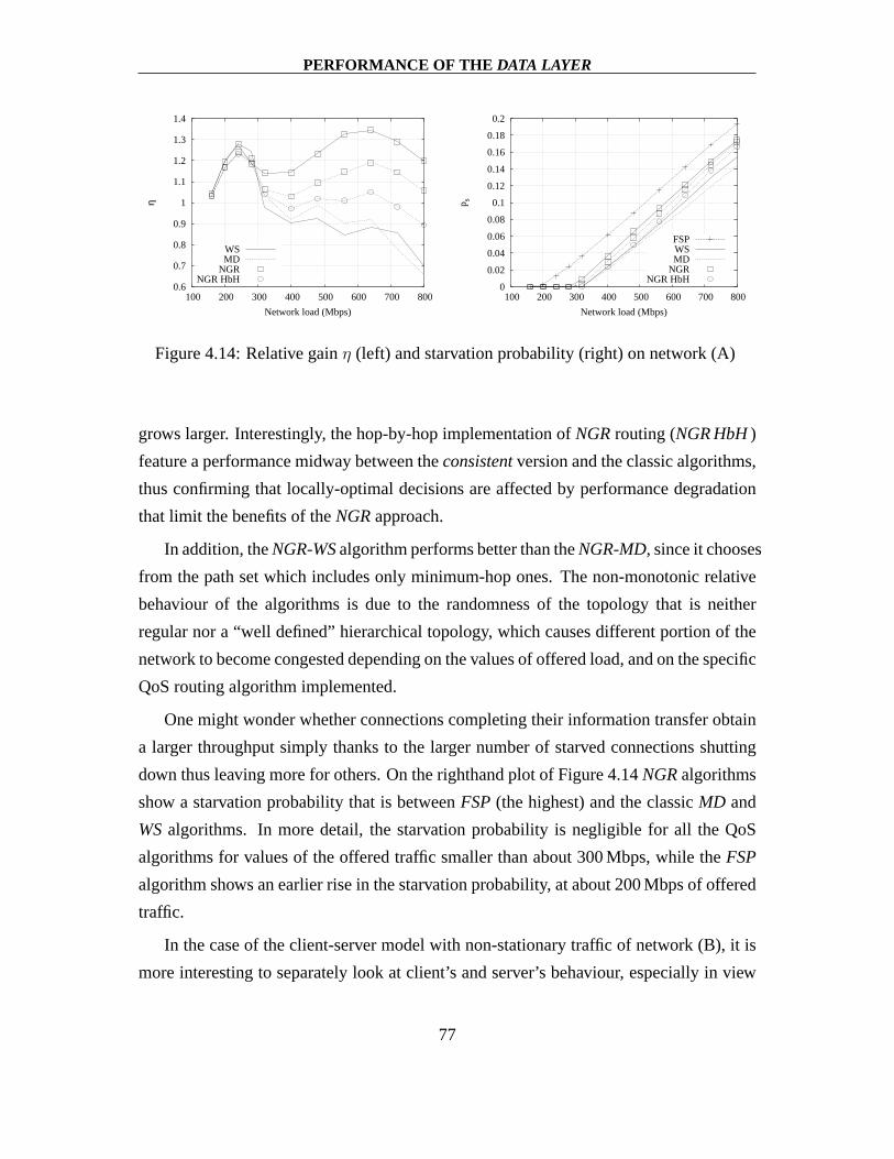
PERFORMANCE OF THE DATA LAYER
0.6
0.7
0.8
0.9
1
1.1
1.2
1.3
1.4
100 200 300 400 500 600 700 800
η
Network load (Mbps)
WSMD
NGRNGR HbH
0
0.02
0.04
0.06
0.08
0.1
0.12
0.14
0.16
0.18
0.2
100 200 300 400 500 600 700 800
p s
Network load (Mbps)
FSPWSMD
NGRNGR HbH
Figure 4.14: Relative gainη (left) and starvation probability (right) on network (A)
grows larger. Interestingly, the hop-by-hop implementation ofNGRrouting (NGR HbH)
feature a performance midway between theconsistentversion and the classic algorithms,
thus confirming that locally-optimal decisions are affected by performance degradation
that limit the benefits of theNGRapproach.
In addition, theNGR-WSalgorithm performs better than theNGR-MD, since it chooses
from the path set which includes only minimum-hop ones. The non-monotonic relative
behaviour of the algorithms is due to the randomness of the topology that is neither
regular nor a “well defined” hierarchical topology, which causes different portion of the
network to become congested depending on the values of offered load, and on the specific
QoS routing algorithm implemented.
One might wonder whether connections completing their information transfer obtain
a larger throughput simply thanks to the larger number of starved connections shutting
down thus leaving more for others. On the righthand plot of Figure 4.14NGRalgorithms
show a starvation probability that is betweenFSP(the highest) and the classicMD and
WSalgorithms. In more detail, the starvation probability is negligible for all the QoS
algorithms for values of the offered traffic smaller than about 300 Mbps, while theFSP
algorithm shows an earlier rise in the starvation probability, at about 200 Mbps of offered
traffic.
In the case of the client-server model with non-stationary traffic of network (B), it is
more interesting to separately look at client’s and server’s behaviour, especially in view
77
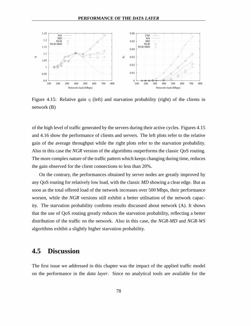
PERFORMANCE OF THE DATA LAYER
0.9
0.95
1
1.05
1.1
1.15
1.2
1.25
100 200 300 400 500 600 700 800
η
Network load (Mbps)
WSMD
NGRNGR HbH
0
0.01
0.02
0.03
0.04
0.05
0.06
100 200 300 400 500 600 700 800
p s
Network load (Mbps)
FSPWSMD
NGRNGR HbH
Figure 4.15: Relative gainη (left) and starvation probability (right) of the clients in
network (B)
of the high level of traffic generated by the servers during their active cycles. Figures 4.15
and 4.16 show the performance of clients and servers. The left plots refer to the relative
gain of the average throughput while the right plots refer tothe starvation probability.
Also in this case theNGRversion of the algorithms outperforms the classic QoS routing.
The more complex nature of the traffic pattern which keeps changing during time, reduces
the gain observed for the client connections to less than 20%.
On the contrary, the performances obtained by server nodes are greatly improved by
any QoS routing for relatively low load, with the classicMD showing a clear edge. But as
soon as the total offered load of the network increases over 500 Mbps, their performance
worsen, while theNGRversions still exhibit a better utilisation of the network capac-
ity. The starvation probability confirms results discussedabout network (A). It shows
that the use of QoS routing greatly reduces the starvation probability, reflecting a better
distribution of the traffic on the network. Also in this case,theNGR-MDandNGR-WS
algorithms exhibit a slightly higher starvation probability.
4.5 Discussion
The first issue we addressed in this chapter was the impact of the applied traffic model
on the performance in thedata layer. Since no analytical tools are available for the
78
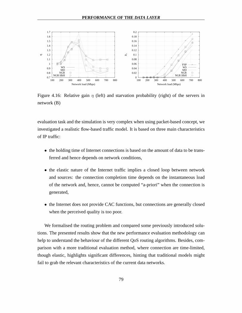
PERFORMANCE OF THE DATA LAYER
0.7
0.8
0.9
1
1.1
1.2
1.3
1.4
1.5
1.6
1.7
100 200 300 400 500 600 700 800
η
Network load (Mbps)
WSMD
NGRNGR HbH
0
0.02
0.04
0.06
0.08
0.1
0.12
0.14
0.16
0.18
0.2
100 200 300 400 500 600 700 800
p s
Network load (Mbps)
FSPWSMD
NGRNGR HbH
Figure 4.16: Relative gainη (left) and starvation probability (right) of the servers in
network (B)
evaluation task and the simulation is very complex when using packet-based concept, we
investigated a realistic flow-based traffic model. It is based on three main characteristics
of IP traffic:
• the holding time of Internet connections is based on the amount of data to be trans-
ferred and hence depends on network conditions,
• the elastic nature of the Internet traffic implies a closed loop between network
and sources: the connection completion time depends on the instantaneous load
of the network and, hence, cannot be computed “a-priori” when the connection is
generated,
• the Internet does not provide CAC functions, but connectionsare generally closed
when the perceived quality is too poor.
We formalised the routing problem and compared some previously introduced solu-
tions. The presented results show that the new performance evaluation methodology can
help to understand the behaviour of the different QoS routing algorithms. Besides, com-
parison with a more traditional evaluation method, where connection are time-limited,
though elastic, highlights significant differences, hinting that traditional models might
fail to grab the relevant characteristics of the current data networks.
79
PERFORMANCE OF THE DATA LAYER
As second issue we analysed the sensitivity of QoS routing algorithms to stale link
state information. A very natural assumption in IP networksis that the information on
resources can not be updated continuously in each node of thenetwork because, on the
one hand, the control traffic grows. On the other hand, the continuous measurements of
link state parameters can be complicated. Thus, the adaptive routing decisions may be
based on inaccurate values. We investigated the problem of how the information update
period influences the performance of adaptive routing algorithms.
Based on the experiences with the traditional ones, we proposed two new classes of
QoS-based routing algorithms. Both of them are robust and combine good performance
with a reduced computational complexity:
• Multimetric Sequential Filtering (MSF) realises a multi–step selection of the suit-
able route. In each step a different type of cost can be considered as ordering basis
and the set of the available paths is halved.
• Network Graph Reduction (NGR) can be applied with any routing algorithms, but
the selection is performed on a special path set. This set consist of paths in the
reduced network graph that contains only uncongested linksplus theFSP path
itself. This concept implicitly realises a load dependent solution.
80

Chapter 5
Analysis of dynamic grooming
5.1 Introduction
In the previous chapters of the dissertation we analysed thedata layerand theoptical
layer in a separated manner. Let us now turn to the complex problem of dynamic groom-
ing, i.e., the interaction of these layers. The aim of this cooperation is the effective usage
of network resources in both layers. While the customers of thedata layerwant a higher
quality in the transmission of their data, the service provider that manages theoptical
layer has different aims. Operators want to provide services without wasting too much
of network capacity and leave free as many resources for further customers as possible.
Traffic grooming helps to resolve this conflict [73]. The goalof using dynamic algo-
rithms is to adapt the virtual topology of thedata layerto the changes of user traffic.
Several solutions have been developed recently, but there are still many open question in
this research area.
As outlined in Section 2.6.4 the application of a theoretical approach for getting in-
sight in the behaviour of IP over WDM networks meets several difficulties. However, we
can extend the results obtained for the optical layer when flow requests that arrive at the
data layerare assumed to require guaranteed bandwidth. With respect to the networks
that allowsubwave channels, Srinivasan et al. introduce a model in [30], that can provide
results considering even inhomogeneous converting capabilities in the nodes. However,
some constraints are still present and the calculation is slow and complex. In [74] Xin
81
ANALYSIS OF DYNAMIC GROOMING
et al. presented an accurate and robust model of traffic grooming analysis considering
alternative paths and first fit wavelength assignment. The complexity is quite high also in
these cases due to the recursive steps of the calculation. In[75] we analysed the problem
by reducing it to a model that was introduced for the analysisof all-optical networks.
This issue is addressed in Section 5.2.
On the other hand, the rather interesting problem is the analysis of the interaction in
the IP scenario, i.e., when thedata layeris modelled to catch the special characteristics
of Internet traffic. Many grooming algorithms were proposedin recent years, see [4,
28, 76, 77] to cite just a few, and compared one another, or simply against a standard
wavelength routed network where no grooming is performed. Some works assume static
grooming [77, 78], and generally tackle the problem with same optimisation technique,
while others assume that grooming is dynamic [5, 28, 79, 80].All these works, however,
simply disregard the elastic nature of TCP/IP traffic: IP overWDM is indeed modelled
like a traditional circuit switched traffic with bandwidth guarantees.
Regarding the results of Section 4.2 we can state that the analysis with a too sim-
ple traffic model may lead to wrong conclusions, since the choice of the model affects
seriously the performance measures. Another weak point of many analysing works is
ignoring the dynamic interaction of the layers that impliesignoring also some extraor-
dinary effects. Our studies presented in [32, 81, 82] instead, give deeper insight in how
grooming schemes may work in realistic IP over WDM networks. Section 5.3 addresses
the problem of considering elastic traffic in dynamic grooming issues.
5.2 Grooming guaranteed traffic
Here we show how the grooming analysis can be reduced to a problem that can be studied
with a theoretical model based onWDMM introduced in Section 3.2. To perform the
reduction we need some specific assumptions on thedata layertraffic and the adaptation
of the model to handle this traffic.
82
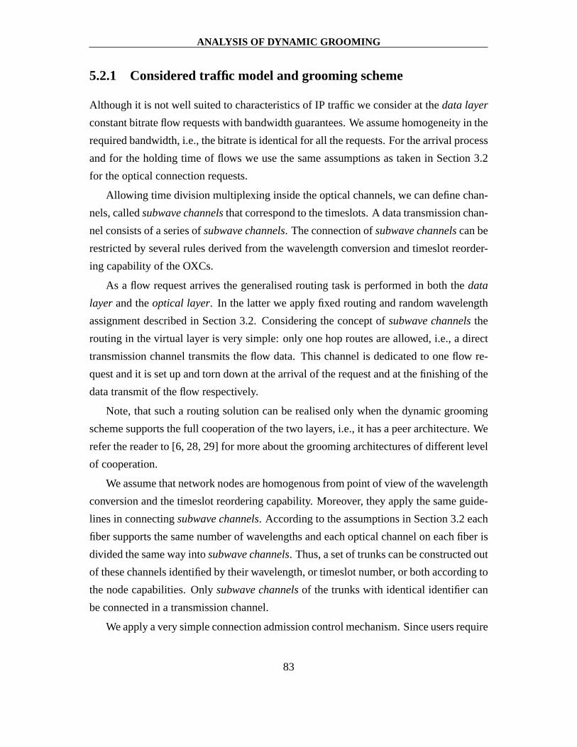
ANALYSIS OF DYNAMIC GROOMING
5.2.1 Considered traffic model and grooming scheme
Although it is not well suited to characteristics of IP traffic we consider at thedata layer
constant bitrate flow requests with bandwidth guarantees. We assume homogeneity in the
required bandwidth, i.e., the bitrate is identical for all the requests. For the arrival process
and for the holding time of flows we use the same assumptions astaken in Section 3.2
for the optical connection requests.
Allowing time division multiplexing inside the optical channels, we can define chan-
nels, calledsubwave channelsthat correspond to the timeslots. A data transmission chan-
nel consists of a series ofsubwave channels. The connection ofsubwave channelscan be
restricted by several rules derived from the wavelength conversion and timeslot reorder-
ing capability of the OXCs.
As a flow request arrives the generalised routing task is performed in both thedata
layer and theoptical layer. In the latter we apply fixed routing and random wavelength
assignment described in Section 3.2. Considering the concept of subwave channelsthe
routing in the virtual layer is very simple: only one hop routes are allowed, i.e., a direct
transmission channel transmits the flow data. This channel is dedicated to one flow re-
quest and it is set up and torn down at the arrival of the request and at the finishing of the
data transmit of the flow respectively.
Note, that such a routing solution can be realised only when the dynamic grooming
scheme supports the full cooperation of the two layers, i.e., it has a peer architecture. We
refer the reader to [6, 28, 29] for more about the grooming architectures of different level
of cooperation.
We assume that network nodes are homogenous from point of view of the wavelength
conversion and the timeslot reordering capability. Moreover, they apply the same guide-
lines in connectingsubwave channels. According to the assumptions in Section 3.2 each
fiber supports the same number of wavelengths and each optical channel on each fiber is
divided the same way intosubwave channels. Thus, a set of trunks can be constructed out
of these channels identified by their wavelength, or timeslot number, or both according to
the node capabilities. Onlysubwave channelsof the trunks with identical identifier can
be connected in a transmission channel.
We apply a very simple connection admission control mechanism. Since users require
83

ANALYSIS OF DYNAMIC GROOMING
bandwidth guarantees, if no suitable path is found, i.e., nodirect channel can be set up,
the request is blocked. As main performance measure we find the blocking probability
defined as the number of blocked requests divided by the number of all requests.
5.2.2 Description of the model
Let us present the extension of theWDMM to aHomogenous Guaranteed-traffic Groom-
ing Model, HGGM . The algorithm of the blocking probability computation does not
change, but some parameters are interpreted in a different way, according to the concept
of subwave channels.
Let us considerbh the bitrate of the connections to be the bandwidth of a transmission
channel. The number ofsubwave channelsin an optical channel equalsU = bCO/bhc,
whereCO is the bandwidth of one whole wavelength. On each links the number of
subwave channeltrunksTSO is equal to:
• C, when only timeslot reordering is allowed,
• U , when only wavelength conversion is allowed,
• 1, when both these functions are enabled,
• C · U , when none of them are allowed.
Each step of the analysis can be performed usingsubwave channeltrunks instead of
wavelength trunks. In the computations we have to use the valueTSO instead ofC and
the valuesCj/TSO instead of the valuesMj.
5.2.3 Numerical results
To evaluate the accuracy of the extended model we compared its results to simulation by
reporting request blocking probability in function of network load. The simulation model
had to be extended to consider the grooming scheme and the concept ofsubwave chan-
nels. The trunk interpretation was changed according to the extension of the theoretical
model.
84
ANALYSIS OF DYNAMIC GROOMING
We analysed the impact of traffic granularity on blocking in regular and irregular
topology scenarios similarly as in Section 3.2.3. Here we show the results network
CWEN presented on Figure 3.5. The link capacity values has to beunderstood this time
in 100 Mbps, e.g., 64 means 6.4 Gbps. Each fiber contains 4 wavelengths of 0.8 Gbps
capacity. We consider neither wavelength conversion nor reordering of timeslots and we
use the same traffic relation matrix as in Section 3.2.3.
1e-04
1e-03
1e-02
48 50 52 54 56 58 60 62 64 66 68
Con
nect
ion
Blo
ckin
g P
roba
bilit
y
Network load (Gbps)
SimulationHGGM 1e-04
1e-03
1e-02
48 50 52 54 56 58 60 62 64 66 68C
onne
ctio
n B
lock
ing
Pro
babi
lity
Network load (Gbps)
SimulationHGGM
Figure 5.1: Blocking probability in the CWEN network, guaranteed bandwidthbh is 100
Mbps (left) and 200 Mbps (right)
First, the guaranteed bandwidth of the flows was 100 Mbps and the left plot of Figure
5.1 reports the results obtained withHGGM and simulation. A different granularity of
the traffic was analysed usingbh equal to 200 Mbps. The results can be seen on the right
plot of Figure 5.1. On these plots the total network load is given in Gbps.
Thanks to the consistent extension of the theoretical and the simulation models we
can observe high accuracy, similarly to the case of theoptical layeranalysis in Section
3.2.3.
5.3 Grooming elastic traffic
Our aim in this section is to investigate how traffic elasticity impacts on some basic
grooming algorithms and assess their performance in dynamic networking scenarios
where theoptical layeranddata layerinteract. Beyond the resource sharing and traf-
85

ANALYSIS OF DYNAMIC GROOMING
fic modelling problem analysed in Section 4.2 we meet also theissue of how the optical
management plan behaves and assigns resources to traffic relations.
5.3.1 Considered models and schemes
As mentioned above, the adaptivity of traffic has a deep impact on the network perfor-
mance and in particular on routing algorithms. The reason lies in the feedback nature
of the interaction of elastic traffic with the network: the network status, e.g. congestion
induces a negative or positive feedback reaction in the source. As usual in closed loop
systems with delay, the nature of feedback, i.e., whether itis positive or negative, can
change with changing conditions. For instance, a negative feedback at low loads can
change to a positive feedback at high loads, leading to instability phenomena.
Considering the foreseen trend of the very dynamic and aggressive use of optical
paths in metro-area optical network and the behaviour of theaggregated flows in more
traditional wide-area optical networks it is easy to derivethat elasticity in groomed traffic
can arise in very different scenarios. To model the elasticity we usedTB andDB model
for thedata layertraffic in the analysis of IP over WDM networks with dynamic traffic
grooming.
Let us concretise more the general network vision of Section2.1. Thedata layeras-
sumes traditional routers with arbitrary routing, that is performed on the virtual topology.
In this topology eachlightpathof theoptical layeris seen as a single hop regardless of the
number of OXCs it crosses. Further, we consider two node architectures: a node can be a
pure OXC which allows to switch entirelightpathsfrom an ingress port to an egress port,
or it can be a Grooming OXC (G-OXC) which supports elastic traffic flows and groom
them onto optical channels and realise also IP router functions. Thedata layertraffic
can then be transmitted or received only in G-OXCs and transittraffic, which does not
terminate in the IP router, can be groomed with incoming traffic. We are not concerned
on the technology (optical or electronic) used for grooming.
In this architecture, a path connecting two routers in the IPlayer is called a virtual or
logical path, because it is created over some establishedlightpathin the optical layer, i.e.,
over virtual links. We assume the overlay grooming architecture [6] that does not allow
the exchange of information between the layers. The consideration of this separated
86

ANALYSIS OF DYNAMIC GROOMING
control is rather realistic in networks where different providers manage the services of
the layers as usual in networks of our days. In this case the routing in thedata layerand
the RWA in theoptical layerwork without any direct interaction. The lack of knowledge
of the actual resource use in the other layer may lead to taking decisions based on a local
optimum that affects negatively later decisions.
Here, the only, but not trivial function of grooming is to decide whether a new traffic
relation must be routed at the IP level, i.e., using the current virtual topology. The other
option is to demand the setup of new virtual links realised byestablishinglightpathsin
theoptical layer. We considered the most cited grooming algorithms introduced in [80]
for CBR traffic, and adopted them to the elastic traffic scenarioas follows:
• Virtual-topology First (VirtFirst). Each time a new IP request arrives in some
router, the current virtual topology is considered first to route the request. If,
once routed, the amount of bandwidth for some flow, not necessarily the one be-
ing routed, is less than a thresholdtho, then if possible, a newlightpath is set-up
between source and destination. If the setup is successful,the IP request is routed
over it and a new virtual topology is computed at thedata layer. The new topology
does not affect already routed requests, i.e., no re-routing is considered, but it will
be used for routing all new requests. If the newlightpath cannot be set up, the
request is routed based on the current virtual topology.
• Optical-level First(OptFirst). Each time a new IP request arrives in some router,
the G-OXC always attempts first to set up a newlightpath in the optical layer, in
order to route the request over it. If no free wavelengths areavailable here, the IP
router routes the incoming request over the current virtualtopology. Indeed, a vir-
tual topology is addressed only when optical resources for the considered source-
destination pair are exhausted.
Since elastic traffic is considered, the upper limit to the possible number of flows
which exist in thedata layerdepends from the minimal acceptable bandwidthbm. How-
ever, this parameter can not be applied directly in grooming, thus the need for the es-
tablishment of a newlightpath in VirtFirst must be introduced based on some suitable
parameter. We define the above referred parameter, calledoptical opening thresholdtho,
as a threshold on the instantaneous throughput obtained by connections.
87

ANALYSIS OF DYNAMIC GROOMING
Whenever a closing flow leaves alightpathempty, thelightpath is closed too and the
virtual topology is re-computed. A generalised formulation and more detailed analysis
of grooming policies with overlay architecture is presented in [82].
5.3.2 Performance measures
To analyse the complex function of dynamic grooming we joined and extended the fea-
tures of the previously used simulation tools ANCLES and ASONCLES. A more detailed
description of the resulting tool GANCLES [39] can be found in[81].
In [32] we derived some results on a trivial topology to demonstrate that dynamic
grooming analysis can lead to surprising results. Since thetheoretical models are of rather
limited generality, here we present only some simulation results to give an illustration of
the performance of such networks. As we will see, the phenomena involved in routing
and grooming elastic traffic are rather complex, and often far from intuitive. To highlight
some basic effects caused by the interaction of grooming algorithms and elastic traffic
we use only very simple routing algorithms both at the optical and at the IP level.
We compared the traffic modelsTBandDB introduced in Section 4.2.3 similarly as in
Section 4.2.5, but in the environment of IP over WDM. Thus, beside the parameters used
in case of a separated analysis of theoptical layeranddata layer, some new parameters
and performance measures have to be considered. Three of them are at the IP level and
three at the optical level:
T : the average throughput per flow as introduced in Section 4.2.5.1,
ps: the starvation probability as introduced in Section 4.2.3.3,
Nl: average number of IP hops per flow,
Nlo: average number of optical hops perlightpath,
Lo: average of the open optical channels per optical link,
Ro: the ratio between the opening rate of optical paths and the arrival rate of flows at
the IP level. It is a measure of the optical level routing effort.
88

ANALYSIS OF DYNAMIC GROOMING
Note that for an optical routed network without groomingRo = 1, while for a network
with static groomingRo = 0.
Clearly, the goal of a grooming algorithm is maximisingT while minimising ps,
Ro and Lo. For the other parameters there are no obvious guidelines onthe optimal
behaviour.
OXC
G−OXC� �� �� �
� �� �� �
� � �� � �� � �� � �� � �
� � �� � �� � �� � �� � �
� � �� � �� � �� � �� � �
� � �� � �� � �� � �� � �
� � �� � �� � �� � �� � �
� � �� � �� � �� � �� � �
� � � �� � � �� � � �� � � �� � � �
� � �� � �� � �� � �� � �
� � �� � �� � �� � �� � �
Figure 5.2: NSFNET network
The dynamic grooming policies were compared in scenarios with regular, e.g. full
mesh and ring, and irregular topologies in [32, 81, 82]. Herewe present results obtained
on the NSFNET network [83] shown in Figure 5.2, which has 13 nodes and 18 fiber
links. Each fiber carry up to 4 wavelengths, and only 6 nodes out of 13 have grooming
capability, i.e., they are G-OXCs. Each wavelength has a capacity of 20 Gbps. A best-
effort traffic source is connected to each G-OXC, opening flowswith BM = 10 Gbps.
Each flow transfers data whose size is randomly chosen from anexponential distribution
with average 12.5 GBytes. A uniform traffic pattern is simulated, ths is set to 0.1 in all
simulations andtho = ths for the sake of simplicity.
The left plot of Figure 5.3 presents a comparison of the average throughputT obtained
by modelling best-effort traffic relations using theTB and theDB approach. Simulations
were performed for bothVirtFirst and OptFirst grooming algorithms. The right plot
reports the starvation probability.
The difference in performance results of the two approachesis striking. Let us con-
sider first theOptFirst grooming policy. Both approaches showT starting from 10 Gbps
when the offered load is low and they immediately diverge as the offered load increases.
89

ANALYSIS OF DYNAMIC GROOMING
2
3
4
5
6
7
8
9
10
0 200 400 600 800 1000 1200
T (
Gbp
s)
Network load (Gbps)
OptFirstVirtfirst
TB modelDB model
1e-06
1e-05
1e-04
1e-03
1e-02
1e-01
1e+00
0 200 400 600 800 1000 1200
p s
Network load (Gbps)
OptFirstVirtfirst
TB modelDB model
Figure 5.3: Average bandwidth per connection (left) and starvation probability (right) for
DB andTBmodels
Indeed, theDB traffic model shows much faster decrease inT as soon as the offered
load increases and this is due to the spreading of congestionover the time with a sort
of avalanche effect mentioned in Section 4.2.5.2. On the contrary, theTB traffic model
shows a smoother decrease of the average bandwidth.
Analysing the starvation probability on the righthand plotof Figure 5.3 adds more
insight. When the traffic is very low, i.e., below 350 Gbps, both traffic models show the
same, very strange behaviour forOptFirst: ps increases and then decreases sharply. This
form of starvation is independent of the traffic model and it is due to a very aggressive
and dynamic use of optical resources of this grooming solution. This greedy policy
leads sometimes to have no connectivity in thedata layerbetween the source and the
destination at flow request arrival. This means, that there is neither any available path in
the virtual topology, nor the possibility to establish a newdirect lightpath in theoptical
layer. Note that this effect of starvation can be interpreted rather as flow request blocking.
However, when the load increaseslightpathsbecome more stable, because there is
always traffic keeping them open. Thus the probability that the virtual topology is not
completely connected becomes negligible. When the load increases further, the two traf-
fic models behaviour diverges: theTBmodel shows no starvation at all, while it increases
steadily in theDB model. This difference in theps behaviour enhances the differences in
T , since aborting flows cause a waste of bandwidth.
When considering theVirtFirst grooming policy instead, the behaviour of both traffic
90

ANALYSIS OF DYNAMIC GROOMING
models is different from the previous one:T decreases sharply even when the offered
load is low, due to the conservative policy. In fact,VirtFirst sets up the minimum number
of lightpaths in order to guarantee the minimum network connectivity, andkeeps this
configuration unchanged until some flow would cross theoptical opening threshold. Only
in this caseVirtFirst increases the resources at IP level by setting up newlightpaths, if
at all possible. In particular, theT for DB traffic model decreases very rapidly, causing
an earlier set-up of newlightpathscompared toTB traffic. This leads the mean assigned
bandwidthT to “bounce” taking advantage of the higher number oflightpaths in the
network. Using the Data-based approach it happens at a load much smaller than for the
Time-based model, that starts increasing again at higher loads. Obviously, both models
show definitive decrease inT for higher loads, not presented here. It is interesting to
notice that the starvation rate for theTB model is in this case always zero apart from
some points at very high loads with aps around10−6. Using theDB modelps increases
steadily and shows a behaviour similar to theDB model with theOptFirst policy.
0.8
1
1.2
1.4
1.6
1.8
2
2.2
0 200 400 600 800 1000 1200
Nh
Network load (Gbps)
OptFirstVirtfirst
TB modelDB model
1.8
1.9
2
2.1
2.2
2.3
2.4
2.5
2.6
2.7
2.8
0 200 400 600 800 1000 1200
Nlo
Network load (Gbps)
OptFirstVirtfirst
TB modelDB model
Figure 5.4: Average number of hopsNl in the data layer(left) andNlo in the optical
layer (right)
The left plot of Figure 5.4 reports the average number of IP hops per flowNl. As
expected theOptFirst policy for bothDB andTB model keeps this parameter close to
one since it attempts to open always directlightpathsbetween the source and destination.
TheVirtFirst for DB traffic instead shows a sharp increase for low loads due to thehigh
probability that a flow arrives and finds the virtual topologyalready connecting the source
91

ANALYSIS OF DYNAMIC GROOMING
and destination. As the load increases,Nl decreases and converges to one because also
theVirtFirst policy starts to open directlightpaths. The same behaviour can be observed
for the Time-based approach but with a smoother peak at a higher load value. This
difference is due to the fact that in theTB case theT of flows decreases smoother and
thusVirtFirst starts to open newlightpathsat higher loads.
Figure 5.4 plots the parameterNlo on the right part. Once again the behaviour of
theOptFirst policy is more predictable, with the number of links that decreases steadily
with the load, and roughly converges to the weighted averagedistance in number of links
between G-OXCs for bothTB andDB. TheVirtFirst policy shows instead longer optical
paths even for high loads. This effect is due to the intrinsicbehaviour of this grooming
policy: most of thelightpathsset up byVirtFirst are in fact never torn-down since they
are carrying traffic almost all the time. On the other hand this policy uses theoptical layer
resources in a conservative way, thus, when a new, longerlightpathmust be established,
it is more likely to find enough free optical channels to set itup. The difference of traffic
models forVirtFirst comes again from the earlier decrease ofT with DB that implies
lightpathsetups.
0
0.5
1
1.5
2
2.5
3
0 200 400 600 800 1000 1200
Lo
Network load (Gbps)
OptFirstVirtfirst
TB modelDB model
1e-05
1e-04
1e-03
1e-02
1e-01
1e+00
0 200 400 600 800 1000 1200
Ro
Network load (Gbps)
OptFirstVirtfirst
TB modelDB model
Figure 5.5: Average optical link loadLo (left) andlightpathopening rateRo (right)
Considering the characteristics discussed above for the different policies and traffic
models, the average numberLo of opened optical channels per link in theoptical layer
plotted on the lefthand side of Figure 5.5 does not present any surprise. The policy
VirtFirst uses a lot of resources with both traffic approaches and converges to a saturated
92

ANALYSIS OF DYNAMIC GROOMING
optical layerat high loads. However, due to the topology, at every time there are some
channels that remain free andLo does not reach the total number of channels in an optical
link. Using VirtFirst the optical link load increases in a less aggressive manner.Lo
converges to that ofOptFirst for the modelDB, while for TB it ends up in a much lower
value.
The right plot of 5.5 shows the ratioRo. As expected, whenVirtFirst grooming policy
is used,Ro decreases quickly with the load, indicating a burden for theoptical level that
does not increase with the traffic. It is interesting to notice the different behaviour of
this parameter between the two traffic models. Using theDB modelVirtFirst shows a
lower and static rate oflightpathopening when the load increases, while forTBwe find a
decreasing and then re-increasing characteristics. When instead, theOptFirst grooming
policy is used,Ro decreases slowly and smoothly, indicating a rather high burden for the
optical level.
Results in other scenarios verified our comments by showing similar behaviour of the
algorithms.
5.4 Discussion
In this chapter we dealt with the problem of dynamic traffic grooming in IP over WDM
networks.
First we show how theWDMM model of Section 3.2 can be extended to study the
grooming of homogenous and guaranteed traffic. The concept of subwave channelslead
us to the derivation of modelHGGM . The model provides accurate approximation of
the connection request blocking probability. However, it is not a very robust solution
and can be applied only for networks with homogenous conversion and multiplexing
characteristics in each nodes.
Second, we presented some initial steps of the analysis of dynamic grooming algo-
rithms with elastic traffic. The research of this area is still in an introductory phase and
the solutions published in the relating works place little attention on how to suit the algo-
rithms to realistic scenarios in IP over WDM networks.
The elasticity of traffic interacts with the grooming algorithms as well as with routing
93
ANALYSIS OF DYNAMIC GROOMING
both at the IP and optical level, leading to unexpected results. Two grooming algorithms,
both using an overlay architecture, have been considered and analysed comparing the
Time- and Data-based approach in the elastic traffic modelling. In both theOptFirst and
VirtFirst grooming algorithms the impact of elastic traffic is dramatic, showing clearly
that approximating IP traffic with a not well suited traffic model can lead to wrong con-
clusions when routing and grooming are considered.
The results for both policies show that they are not appropriate to manage the two-
layer network due to the lack of layer coordination in the overlay architecture. On the
one hand, usingOptFirst, it can lead to wasting resources inoptical layer, that may
cause even request blocking due to not completely connectedvirtual topology. On the
other hand, usingVirtFirst, the conservative guidelines applied to set up a new virtual
link may lead to low quality of data transport at thedata layer.
94

Chapter 6
Conclusion
In the PhD dissertation we addressed the problem of the performance analysis of the
general routing solution in IP over WDM networks, including the routing algorithms in
both layers and the grooming policies. This task was separated into three subtasks and
analysed with different methods.
First, in Chapter 3 theoptical layerwas studied. We introduced theWDMM the-
oretical model that calculates the blocking probability ofoptical connection requests in
multifiber optical networks without wavelength conversion. The results show the rather
low complexity of the computation algorithm and the accuracy of the model.
However, in the case of low load and long routes assigned to the connections some
inaccuracy can be observed, thus further refinement of the model is required. On the other
hand,WDMM shall be extended to support more general traffic models, RWAsolutions
and network architectures.
Second, Chapter 4 dealt with the analysis of thedata layer. Two flow-based traffic
models representing elasticity and a model for flow starvation were introduced and tested
with known routing algorithms. Simulation results show theclear difference of theTB
andDB approaches proving that a simple traffic model fails in the performance analysis
and may lead to wrong conclusions.
We studied also the impact of stale link state information onthe performance of the
dynamic routing solutions. We found a strong degradation when the link state update
frequency decreases and proposedMSF, a new class of routing based on multiple filtering
of available paths. Some of these algorithms resist to the degrading effects caused by the
95

CONCLUSION
large update periods. Another group of QoS routing algorithmsNGR was developed to
realise a kind of built-in load dependence by avoiding heavily loaded segments of the
network. We found that the routing solutions adopting the concept of network graph
reduction during the path selection process allow good performance for high network
load as well, even in complex scenarios.
Third, the compound IP over WDM network scenario was studied in Chapter 5 re-
garding the interaction ofdata layerandoptical layerwhen assuming dynamic grooming.
In the first part of the chapter we proposedHGGM , a theoretical model that considers
requests with bandwidth guarantees. In the case of this model several constraints of ap-
plicability have to be loosed.
The second part presents the study of grooming policies of overlay architecture in
elastic traffic scenarios. We found again the striking difference between theTB and
DB traffic models in thedata layerand highlighted some special behaviours due to the
grooming policy characteristics. A further analysis of this issue can help us to determine
the roots of all the observed effects and to design new algorithms that suit better to this
environment. A possible direction of further research is the definition and analysis of new
performance measures. To generalise our studies, the observation of dynamic grooming
policies of more complex architectures and combined with different routing algorithms
in theoptical layeranddata layeris required.
96
Bibliography
[1] R. Ramaswami and K. N. Sivarajan. Routing and wavelength assignment in all-
optical networks.IEEE/ACM Transactions on Networking, 3(5):489–500, 1995.
[2] G. Apostolopoulos, R. Guerin, S. Kamat, and S. K. Tripathi. Quality of service
based routing: A performance perspective. InProc. of ACM SIGCOMM’98, 1998.
Vancouver, Canada.
[3] E. Karasan and E. Ayanoglu. Effects of wavelength routing and selection algorithms
on wavelength conversion gain in wdm optical networks.IEEE/ACM Transactions
on Networking, 6(2):186–196, 1998.
[4] R. Dutta and G. N. Rouskas. Traffic grooming in wdm networks:past and future.
IEEE Network Magazine, 16(6):46–56, 2002.
[5] R. Srinivasan and A. K. Somani. Dynamic routing in wdm grooming networks.
Photonic Network Communications, 5(2):123–135, 2003.
[6] B. Rajagopalan, J. Luciani, and D. Awduche. RFC 3717: IP overoptical networks:
A framework, March 2004.
[7] A. Jajszczyk. Optical networks - the electro-optic reality. Optical Switching and
Networking, 1(1):3–18, 2005.
[8] B. Craignou, R. Clemente, J. Robaday, L. Jereb, Z. Ioannidis, and J. Santos. Net-
work operator perspectives on optical networks - evolutiontowards ason. InProc.
of Networks 2002, June 2002. Munich, Germany.
97
BIBLIOGRAPHY
[9] Eurescom P1012, Flexible Automatic SwitcHed Optical Networks.
http://www.eurescom.de/public/projects/P1000-series/p1012/.
[10] H. Harai, M. Murata, and H. Miyahara. Performance analysis of wavalength as-
signment policies in all-optical networks with limited-range wavelength conversion.
IEEE Journal on Selected Areas in Communications, 16(7):1051–1060, 1998.
[11] et al. Kaminow, I. P. A wideband all-optical wdm network. IEEE Journal on
Selected Areas in Communications, 14(5):780–799, 1996.
[12] S. Subramaniam, A. K. Somani, M. Azizoglu, and R.A. Barry.A performance
model for wavelength conversion with non-poisson traffic. In Proc. of IEEE INFO-
COM’97, pages 499–506, April 1997.
[13] Zoltan Zsoka. Ason halozatok forgalmanak modellezese. InProc. of HTE-BME
2002 diakkonferencia, May 2002. Budapest, Hungary.
[14] S. Shenker and J. Wroclawski. RFC 2216: Network element service specification
template, September 1997.
[15] S. Blake, D. Black, M. Carlson, E. Davies, Z. Wang, and W. Weiss. RFC 2475: An
architecture for Differentiated Services, December 1999.
[16] J. Roberts. Traffic theory and the internet.IEEE Communications Magazine,
39(1):94–99, 2001.
[17] S. Shakkottai, A. Kumar, A. Karnik, and A. Anvekar. Tcp performance over end-
to-end rate control and stochastic available capacity.IEEE/ACM Transactions on
Networking, 9(4):377–391, 2001.
[18] S. Racz, B. P. Gero, and G. Fodor. Flow level performance analysis of a multi-
service system supporting elastic and adaptive services.Performance Evaluation,
49(1-4):451–469, 2002.
[19] A. A. Kherani and A. Kumar. Stochastic models for throughput analysis of ran-
domly arriving elastic flows in the internet. InProc. of IEEE INFOCOM’02, 2002.
98
BIBLIOGRAPHY
[20] Q. Ma and P. Steenkiste. Routing traffic with quality-of-service guarantees in in-
tegrated services networks. InProc. of 8th IEEE/ACM International Workshop on
Network and Operating Systems Support for Digital Audio and Video (NOSSDAV
1998), July 1998. England.
[21] A. Shaikh, J. Rexford, and K.G. Shin. Load-sensitive routing of long-lived ip flows.
In Proc. of ACM SIGCOMM’99, pages 215–226, August 1999. Cambridge, MA
USA.
[22] C. Casetti, G. Favalessa, M. Mellia, and M. M. Munafo. An adaptive routing algo-
rithm for best-effort traffic in integrated-services networks. In Proc. of 16th Inter-
national Teletraffic Congress, IEE ITC-16, June 1999. Edinburgh, UK.
[23] C. Casetti, R. Lo Cigno, M. Mellia, M. M. Munafo, and Zoltan Zsoka. A new class
of qos routing strategies based on network graph reduction.Computer Networks,
41(4):475–487, 2003.
[24] R. Gu’erin and A. Orda. Qos-based routing in networks with inaccurate informa-
tion. In Proc. of IEEE INFOCOM’97, April 1997. Kobe, Japan.
[25] G. Apostolopoulos, R. Guerin, S. Kamat, and S. K. Tripathi. Improving qos routing
performance under inaccurate link state information. InProc. of 16th International
Teletraffic Congress, IEE ITC, June 1999. Edinburgh, UK.
[26] A. Shaikh, J. Rexford, and K.G. Shin. Evaluating the impact of stale link state on
quality-of-service routing.IEEE/ACM Transactions on Networking, 9(2):162–176,
2001.
[27] S. Sibal and A. De Simone. Controlling alternate routingin general-mesh packet
flow networks. InProc. of ACM SIGCOMM’94, August 1994. London, UK.
[28] H. Zhu, H. Zang, K.Zhu, and B. Mukherjee. A novel generic graph model for
traffic grooming in heterogeneous wdm mesh networks.IEEE/ACM Transactions
on Networking, 11(2):285–299, 2003.
99

BIBLIOGRAPHY
[29] S. Koo, G. Sahin, and S. Subramaniam. Dynamic lsp provisioning in overlay, aug-
mented, and peer architectures for ip/mpls over wdm networks. In Proc. of IEEE
INFOCOM’04, Mar. 7-11 2004. Hong Kong, China.
[30] R. Srinivasan and A. K. Somani. Analysis of optical networks with heterogeneous
grooming architectures.IEEE/ACM Transactions on Networking, 12(5):931–943,
2004.
[31] R. Lo Cigno, E. Salvadori, D. Severina, and Z. Zsoka. GANCLES: A network
level simulator to study optical routing, wavelength assignment and grooming algo-
rithms. Technical Report DIT-04-017, DIT - University of Trento, 2004.
[32] R. Lo Cigno, E. Salvadori, and Z. Zsoka. Elastic traffic effects on wdm dynamic
grooming algorithms. InProc. of IEEE GLOBECOM’04, Nov. 29 - Dec. 3 2004.
Dallas, Texas USA.
[33] L. Kleinrock. Queueing Systems. John Wiley, 1976.
[34] T.G. Robertazzi.Computer Networks and Systems: Queueing Theory and Perfor-
mance Evaluation. Springer, 2000.
[35] D. Bertsekas and R. Gallager.Data Networks. Prentice Hall, 1992.
[36] M. Ajmone Marsan, A. Bianco, C. Casetti, C. F. Chiasserini, A.Francini, R. Lo
Cigno, and M. M. Munafo. An integrated simulation environment for the analy-
sis of atm networks at multiple time scales.Computer Networks and ISDN Sys-
tems, Special Issue on Modeling of Wired - and Wireless - ATM Networks, 29(17-
18):2165–2185, 1998.
[37] ANCLES - A Network Call-Level Simulator.
http://www.tlc-networks.polito.it/ancles.
[38] ASONCLES - ASOn Network Call-Level Simulator.
http://www.hit.bme.hu/ zsoka/asoncles.
[39] GANCLES - Gmpls cApable Network Call-Level Simulator.
http://ardent.unitn.it/gancles.
100

BIBLIOGRAPHY
[40] C. Casetti, R. Lo Cigno, M. Mellia, M. M. Munafo, and Zoltan Zsoka. Qos routing
strategies when link state information is out-of-date. InProc. of 8th IFIP Workshop
on Performance Modelling and Evaluation of ATM and IP Networks, July 17-19
2000. Ilkley, West Yorkshire U.K.
[41] C. Casetti, R. Lo Cigno, M. Mellia, M. M. Munafo, and Zoltan Zsoka. A realistic
model to evaluate routing algorithms in the internet. InProc. of IEEE GLOBE-
COM’01, Nov. 25-29 2001. San Antonio, Texas USA.
[42] T. Yung, J. Martin, M. Takai, and R. Bagrodia. Integrationof fluidbased analytical
model with packet-level simulation for analysis of computer networks. InProc.
of Internet Performance and Control of Network Systems II, volume 4523, pages
130–143, 2001. Denver, CO USA.
[43] F. P. Kelly. Charging and rate control for elastic traffic. European Transactions on
Telecommunications, 8(1):33–37, 1997.
[44] Chiu. Some observations on fairness of bandwidth sharing. In Proc. of ISCC 2000.
Fifth IEEE Symposium on Computers and Communications, July 2000.
[45] G. de Veciana, T. Konstantopoulos, and Tae-Jin Lee. Stability and performance
analysis of networks supporting elastic services.IEEE Journal on Selected Areas
in Communications IEEE/ACM Transactions on Networking, 9(1):2–14, 2001.
[46] L. Li and A. K. Somani. Dynamic wavelength routing usingcongestion and
neighborhood information.IEEE/ACM Transactions on Networking, 7(5):779–786,
1999.
[47] H. Zang, J. P. Jue, and B. Mukherjee. A review of routing and wavelength assign-
ment approaches for wavelength-routed optical wdm networks. Optical Networks
Magazine, 1(1):47–60, 2000.
[48] Y. Yoo, S. Ahn, and C. S. Kim. Adaptive routing considering the number of avail-
able wavelengths in wdm networks.IEEE Journal on Selected Areas in Communi-
cations, 8(21):1263–1273, 2003.
101
BIBLIOGRAPHY
[49] R. Barry and P. Humblet. Models of blocking probability inall-optical networks
with and without wavelength changers. InProc. of IEEE INFOCOM’95, April
1995. Boston, US.
[50] S. Subramaniam, M. Azizoglu, and A. Somani. All-optical networks with sparse
wavelength conversion.IEEE/ACM Transactions on Networking, 4(4):544–557,
1996.
[51] L. Li and A. K. Somani. Blocking performance analysis of fixed-paths least-
congestion routing in multifiber wdm networks. InProc. of SPIE Photonics East’99,
pages 56–67, September 1999. Boston, MA USA.
[52] L. Li and A. K. Somani. A new analytical model for multi-fiber wdm networks.
IEEE Journal on Selected Areas in Communications, 18(10):2138–2145, 2000.
[53] A. Birman. Computing approximate blocking probabilities for a class of all-optical
networks. IEEE Journal on Selected Areas in Communications, 14(5):852–857,
1996.
[54] S. Subramaniam, A. K. Somani, M. Azizoglu, and R. A. Barry.The benefits of
wavelength conversion in wdm networks with non-poisson traffic. IEEE Communi-
cations Letters, 3(3):81–83, 1999.
[55] Y. Zhu, G. Rouskas, and H. Perros. A path decomposition approach for computing
blocking probabilities in wavelength routing networks.IEEE/ACM Transactions on
Networking, 8(6):747–762, 2000.
[56] A. Mokhtar and M. Azizoglu. Adaptive wavelength routing in all-optical networks.
IEEE/ACM Transactions on Networking, 6(2):197–206, 1998.
[57] R. Srinivasan and A. K. Somani. A generalized framework for analyzing time-
space switched optical networks. InProc. of IEEE INFOCOM’01, April 2001.
Anchorage, USA.
[58] A. Sridharan and K. N. Sivarajan. Blocking in all-optical networks. InProc. of
IEEE INFOCOM’00, March 2000. Tel-Aviv, Israel.
102

BIBLIOGRAPHY
[59] Zoltan Zsoka. Blocking probability of all-optical multifiber networks. In Proc. of
7th IFIP Working Conference on Optical Network Design and Modelling, ONDM
2003, February 3-5 2003. Budapest, Hungary.
[60] COST239 homepage. http://www.ita.hsr.ch/cost239/.
[61] A. Fumagalli, I. Cerutti, M. Tacca, F. Masetti, R. Jagannathan, and S. Alagar. Sur-
vivable networks based on optimal routing and wdm self-healing rings. InProc. of
IEEE INFOCOM’99, March 1999. New York, NY USA.
[62] E. Rosen, A. Viswanathan, and R. Callon. RFC 3031: Multiprotocol Label Switch-
ing architecture, January 2001.
[63] D. Cavendish and M. Gerla. Internet qos routing using thebellman-ford algorithm.
In Proc. of IFIP Conference on High Performance Networking, HPN 1998, 1998.
Vienna, Austria.
[64] G. Apostolopoulos, D. Williams, S. Kamat, R. Guerin, A. Orda, and T. Przygienda.
RFC 2676: QoS routing mechanisms and OSPF extensions, August1999.
[65] C. Casetti, R. Lo Cigno, M. Mellia, M. M. Munafo, and Zoltan Zsoka. Routing
algorithms evaluation for elastic traffic. InProc. of IEEE Workshop on High Per-
formance Switching and Routing, HPSR 2001, May 29-31 2001. Dallas, Texas
USA.
[66] C. Casetti, R. Lo Cigno, M. Mellia, M. M. Munafo, and Zoltan Zsoka. A new
class of qos routing strategies based on network graph reduction. In Proc. of IEEE
INFOCOM’02, June 23-27 2002. New York, NY USA.
[67] Q. Ma, P. Steenkiste, and H. Zhang. Routing high-bandwidth traffic in max-min fair
share networks. InProc. of ACM SIGCOMM’96, August 1996. Stanford, Canada.
[68] A. Arvidsson and P. Karlsson. On the traffic models for tcp/ip. In Proc. of 16th
International Teletraffic Congress, IEE ITC-16, June 1999. Edinbourgh, UK.
[69] Z. Wang and J. Crowcroft. Qos routing for supporting resource reservation.IEEE
Journal on Selected Areas in Communications, 14(7):1288–1294, 1996.
103

BIBLIOGRAPHY
[70] GT-ITM: Georgia Teach-Internetwork Topology Models.
http://www.cc.gatech.edu/project/gtitm.
[71] C. Casetti, R. Lo Cigno, and M. Mellia. Qos-aware routing schemes based on
hierarchical load-balancing for integrated services packet networks. InProc. of
International Communication Conference, IEEE ICC’99, June 1999. Vancouver,
Canada.
[72] J. L. Sobrinho. Algebra and algorithms for qos path computation and hop-by-hop
routing in the internet.IEEE/ACM Transactions on Networking, 10(4):541–550,
2002.
[73] T. Cinkler. Traffic and lambda grooming.Network, 17(2):16–21, 2003.
[74] C. Xin. Computing blocking probability of dynamic trafficgrooming in mesh wdm
optical networks. InProc. of First International Conference on Broadband Net-
works, 2004. BroadNets 2004, October 2004.
[75] Zoltan Zsoka. Dinamikus forgalomkotegeles (grooming) analızise optikai
halozatokban.Magyar Tavkozles, 15(2):33–37, 2004.
[76] X. Zhang and C. Qiao. An effective and comprehensive approach to traffic groom-
ing and wavelength assignment in sonet/wdm rings.IEEE/ACM Transactions on
Networking, 8(5):608–617, 2000.
[77] K. Zhu and B. Mukherjee. Traffic grooming in an optical wdmmesh network.IEEE
Journal on Selected Areas in Communications, 20(1):122–133, 2003.
[78] M. Brunato and R. Battiti. A multistart randomized greedy algorithm for traffic
grooming on mesh logical topologies. InProc. of 6th IFIP Working Conference
on Optical Network Design and Modelling, ONDM 2002, February 2002. Torino,
Italy.
[79] M. Kodialam and T. V. Lakshman. Integrated dynamic ip and wavelength rout-
ing in ip over wdm networks. InProc. of IEEE INFOCOM’01, Apr. 22-26 2001.
Anchorage, USA.
104

BIBLIOGRAPHY
[80] X. Niu, W. D. Zhong, G. Shen, and T. H. Cheng. Connection establishment of label
switched paths in ip/mpls over optical networks.Photonic Network Communica-
tions, 6(1):33–41, 2003.
[81] R. Lo Cigno, E. Salvadori, and Z. Zsoka. Dynamic grooming in overlay networks:
A study with realistic traffic based on gancles simulation package. InProc. of 9th
IFIP TC6 Conference on Optical Network Design and Modelling, ONDM2005,
February 7-9 2005. Milano, Italy.
[82] R. Lo Cigno, E. Salvadori, and Z. Zsoka. Dynamic grooming in ip over optical
networks based on the overlay architecture.submitted to Optical Switching and
Networking.
[83] O. Crochat and J. Boudec. Design protection for wdm optical networks. IEEE
Journal on Selected Areas in Communications, 16(7):1158–1165, 1998.
105