Zero-Sum Stochastic Games An algorithmic review

Algorithms for competitive games

Zero-Sum Stochastic GamesAn algorithmic review

Emmanuel Hyon LIP6/Paris Nanterrewith N Yemele and L Perrotin

Rosario November 2017Final Meeting DygameDygame Project Amstic


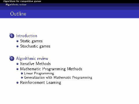
Outline

1 IntroductionStatic gamesStochastic games

2 Algorithmic reviewIterative MethodsMathematic Programming Methods

Linear Programming

Generalization with Mathematic Programming

Reinforcement Learning


Introduction

Static games

Static game de�nition

A static game under a strategic form with complete information isthe 3-uple (N , {Ai}i ,Ri ) where

N is the (�nite) set of players (size N).

Ai is the set of action ai of player i (size mi ).

R i (a) is the reward of player i ,with a = (a1, . . . aN) the set of the actions played by theagents

A strategy is said :

pure strategy : when the selection of the action isdeterministic.

mixed strategy : when each of the action receive a probabilityto be chosen :in this case πi (aij) is the probability of player i to play aij .


Introduction

Static games

Static game de�nition II

The Utility of agent i is

r i (πi , π−i ) =∑ai∈Ai

∑a−i∈A−i

R(ai , a−i )πi (ai )π−i (a−i ). (1)

Dé�nition (Pure Nash Equilibrium)

A set of pure strategies a∗ is a Nash Equilibrium if, for all i ,

R(ai∗, a−i

∗) ≥ R(ai , a−i

∗) ∀ ai ∈ Ai

Dé�nition (Mixed Nash Equilibrium)

A set π∗ of mixed strategies is a Nash Equilibrium if, for all i ,

r(πi∗, π−i

∗) ≥ r(πi , π−i

∗) ∀ πi


Introduction

Static games

Zero-Sum static games

Zero-Sum game : the sum of the utilities of all players is null.

Two players Zero-Sum game : the reward of a player 1 is equal tothe loss of player 2 i.e. ∀a1, a2 R1(a1, a2) = −R2(a1, a2).

Letting, r(π1, π2) = r1(π1, π2). In a two players ZS game if(π1∗, π2∗) form a Nash Equilibrium they satis�es

r(π1, π2∗) ≤ r(π1

∗, π2∗) ≤ r(π1

∗, π2) ∀π1π2 .

and are called Optimal strategies.

Théorème (Minimax (Von Neuman))

A 2 player ZS Game has a value V if and only if

maxπ1

minπ2

r(π1, π2) = minπ2

maxπ1

r(π1, π2) = V


Introduction

Static games

Static Games and linear Programming

[Filar and Vrieze 96], when solving Minimax equation one canrestrict to extreme points :

maxπ1

minπ2

∑i

∑j

π1(i)π2(j)R(a1i , a2

j ) = maxπ1

minj

∑i

π1(i)R(a1i , a2

j )

Player 1 should then solve

maxminj

∑i

π1(i)R(a1i , a2

j )

s.c.∑i

π1(i) = 1

π1(i) ≥ 0 ∀i .

max v

s.c. v ≤∑i

π1(i)R(a1i , a2

j ) ∀ j∑i

π1(i) = 1

π1(i) ≥ 0 ∀i .


Introduction

Stochastic games

Stochastic Games description

We assume

A dynamic game states of which changes over time

A game di�erent in each state

Simultaneous actions of players

A function describes the dynamic evolution of the system w.r.tthe simultaneous plays and the state

When the evolution function is random it is a stochastic game.

Dé�nition (Information Models)

Perfect Information The players knows the set of actions, states

and rewards until step t − 1.

Closed Loop The player knows the the current state of the game


Introduction

Stochastic games

Stochastic Games de�nition

A stochastic game is a 5-uple (N ,S,A,R,P) with :

N is the (�nite) set of player (size N),

S is the state space (size S),

A = {Ai}i∈{1,...,N} is the set of all actions where Ai is the set

of actions ai of player i (size mi ),

Ri is the instantaneous reward of player i .Ri (s, a

1, . . . , aN) depends on state and actions of players

P the transition probability p(s ′|s, a) to switch in state s ′ froms when a = (a1, . . . , aN) is played.

Small Taxonomy :Stochastic Game : transition function depends on the historyMarkov Game : transition function depends on the stateCompetitive Game : 2 player Zero Sum Markov Game


Introduction

Stochastic games

Perfect Nash Equilibrium

Strategy : the strategy πi of player i is the vector |S | ×mi

πi = (πi1, . . . , πiS) with π

i1the mixed strategy on action in state 1.

Expected utility r ik(s, π) is the expected instantaneous reward in sat step k w.r.t π = (π1, . . . , πN).

The Utility of player i in state s is vi (s, π) (γ the discount factor) :

vi (s, π) = Es

∞∑t=0

γ it(r ik(s, π))

t .

Dé�nition (Nash Equilibrium in stochastic game)

A set of strategies π∗ = (π1∗, . . . , πN

∗) is a N.E. if, ∀s ∈ S and ∀i :

vi (s, π∗) ≥ vi (s, π

1∗, . . . , πi−1∗, πi , πi+1∗, . . . , πN

∗) ∀πi

Interested by Perfect Nash Equilibrium = N.E. of any sub-games


Introduction

Stochastic games

Competitive Games

A competitive game is a 2 players Markov Game.It is a discounted gameIt is a Zero Sum game

r1(s, a1, a2) + r2(s, a1, a2) = 0, ∀s ∈ S, a1 ∈ A1(s), a2 ∈ A2(s).

The strategies studied are the Markov Stationary Policies than forstatic

We have the equivalent de�nition of optimal strategies

v(π1, π20) ≤ v(π10, π2

0) ≤ v(π10, π2) .


Introduction

Stochastic games

Shapley Equation

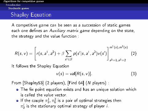
A competitive game can be seen as a succession of static gameseach one de�nes an Auxiliary matrix game depending on the state,the strategy and the value function :

R(s, v) =

[r(s, a1, a2) + β

∑s′∈S

p(s ′|s, a1, a2)v(s ′)

]m1(s),m2(s)

a1=1,a2=2

(2)

It follows the Shapley Equation

v(s) = val[R(s, v)]. (3)

From [Shapley53] (2 players), [Find 64] (N players) :

The �x point equation exists and has an unique solution whichis called the value vector.If the couple π1

0, π2

0is a pair of optimal strategies then

πi0is the stationary optimal strategy of player i .


Algorithmic review

Outline

1 IntroductionStatic gamesStochastic games

2 Algorithmic reviewIterative MethodsMathematic Programming Methods

Linear Programming

Generalization with Mathematic Programming



Algorithmic review

Iterative Methods

Initial Shapley Algorithm

Step 1 Start with any v0 : ∀s, v0(s) has any valueStep 2

Repeat

for s ∈ S do :-Build auxiliary game R(s, vn−1)[r(s, a1, a2) + β

∑s′∈S p(s

′|s, a1, a2)v(s ′)].

-Compute (with Shapley Snow method) the valueand let vn(s) = val [R(s, vn−1)]

end foruntil ‖vn(s)− vn−1(s)‖ < ε ∀sStep 3

for s ∈ S do :- Let v(s) = vn(s), Build R(s, v)- Compute π1(s) et π2(s) π(s) for game R(s, v)

end forreturn v(s), π1(s), π2(s) ∀s.


Algorithmic review

Iterative Methods

Shapley Algorithm with linear Programming

Step 1 Start with any v0 : ∀s, v0(s) has any valueStep 2

Repeat

for s ∈ S do :-Build auxiliary game R(s, vn−1)[r(s, a1, a2) + β

∑s′∈S p(s

′|s, a1, a2)v(s ′)].

-Compute with LP the value and let vn(s) = val [R(s, vn−1)]val [R(s, vn−1)] = maxπ1 mina2∈A2

∑a1 R(s, a

1, a2)π1(a1).end for

until ‖vn(s)− vn−1(s)‖ < ε ∀sStep 3

for s ∈ S do :- Let v(s) = vn(s), - Build R(s, v)- Compute (with LP) π1(s) et π2(s) π(s) for game R(s, v)

end forreturn v(s), π1(s), π2(s) ∀s.


Algorithmic review

Iterative Methods

Ho�man Karp Algorithm

Step 1 Start with approximation v0(s) = 0 ∀s.Step 2 At step nBuild matrix R(s, vn−1)For all s,Find π2n(s) an optimal strategy of R(s, vn−1) for player 2

Step 3

For all s solve the MDPvn(s) = maxπ1 vβ(s, π

1, π2n(s))Step 4

if ‖vn − vn−1‖ > εThen n = n + 1 and go to step 2else stop and return v = vn, π

2 = π2n and π1.


Algorithmic review

Iterative Methods

Pollacheck-Avi Itzak Algorithm

Step 1 Start with arbitrary approximation of v0 :∀s, v0(s) has any value.

Step 2 At step n, the value vn−1 is known.For s ∈ S doBuild matrix R(s, vn−1)Compute the two optimal strategies of game [R(s, vn−1)]let π1n and π2n be these two strategies

Step 3

Compute the value of the gamevn = [I − βP(π1n, π2n)]−1r(π1n, π2n).

Step 4

If π1n = π1n−1 and π1n = π2n−1) then stopelse go to step 2


Algorithmic review

Iterative Methods

Remind on Modi�ed Policy Iteration

In Markov Decision Process Framework, Modi�ed Policy Iteration isa variant of Policy Iteration that avoid to solve a linear system.Step 1 Start with any v0Step 2 At step nFor all s,Find the optimal deterministic Markov policy

πn is an optimal strategy of game R(s, vn−1)Step 3 (in the classical PI algorithm)Compute the value of the gamevn = [I − βP(πn)]−1r(π).

Step 3 (in the Modi�ed Policy Iteration)Approximate the value of the game

u0 = vn−1 Repeat uk = R(s, uk−1)until k = m vn = um Step 4

If πn = πn−1 then stopelse go to step 2


Algorithmic review

Iterative Methods

van der Wal Algorithm (78)

Step 1 Start with v0 such that R(s, v0) ≤ v0(s) ∀s.Step 2 At step nBuild matrix R(s, vn−1)For all s,Find π2n(s) an optimal strategy of game R(s, vn−1)

Step 3

For all s approximate the MDP solutionRepeat m timesv = vn−1vn+1(s) = maxπ1 vβ(s, π

1, π2n(s))vn = vm

Step 4

If ‖vn − vn−1‖ > ε n = n + 1 go to step 2Else stop and return


Algorithmic review

Mathematic Programming Methods

Remind on MDP and Linear Programming

We search maxπ∈Π vπ satisfying the D.P. equation

v(s) = maxa

(r(s, a) + β

∑s′∈S

p(s ′|s, a)v(s ′)

), ∀s ∈ S .

Since (L is the Bellman Operator), if v ≥ Lv then v ≥ v∗ and then∑s v(s) ≥

∑s v∗(s). We can solve the problem by minimizing the

sum insuring the respect of the constraints v ≥ Lv .We get the primal [Filar96]

minv∈ν

S∑s=1

1

Sv(s) (Pβ)

with the set of constraints :

v(s) ≥ r(s, a) + βS∑

s′=1

p(s ′|s, a)v(s ′), ∀a ∈ A(s) , ∀s ∈ S.


Algorithmic review


Single Controller Game

We consider a game in which transitions are controlled only byplayer 1. It has the property than

p(s ′|s, a1, a2) = p(s ′|s, a1), (4)

for all s, s ′ ∈ S, a1 ∈ A1(s), a2 ∈ A2(s).

Fact 1. In the game [R(s, v)], the coordinate with index a1, a2 canbe expressed by :

r(s, a1, a2) + β∑s′∈S

p(s ′|s, a1)v(s ′) .

Fact 2. With the optimal strategies Equation, we have

v(π1(s), π20(s)) ≤ v(π10(s), π2

0(s))

for any π1(s) and namely for all pure strategies (i.e. actions).


Algorithmic review


Single Controller Game (Primal)

Fact 1 and Fact 2 gives

vβ ≥∑a2

π20(s, a2)r(s, a1, a2) + β

∑s′∈S

p(s ′|s, a1)vβ(s ′) ∀s, a1.

This leads to the Primal formulation

minS∑

s′=1

1

Sv(s

′) (Pβ(1))

under constraints :

(a) v(s) ≥∑m2(s)

a2=1r(s, a1, a2)π2(s, a2) +

βS∑

s′=1

p(s ′|s, a1)v(s ′), ∀ s ∈ S, ∀ a1 ∈ A1(s),

(b)∑

a2∈A2(s)

π2(s, a2) = 1, ∀ s ∈ S,

(c) π2(s, a2) ≥ 0, ∀ s ∈ S.


Algorithmic review


Single Controller Game (Dual)

maxS∑

s=1

z(s) (Dβ(1))

under constraints :

d)S∑

s=1

∑a1∈A1(s)

[δ(s, s′)− βp(s ′ |s, a1)]xs a1 =

1

S, ∀ s ′ ∈ S ,

e) z(s) ≤m1(s)∑a1=1

r(s, a1, a2)x(s, a1) , ∀ s ∈ S , ∀ a2 ∈ A2(s) ,

f) x(s, a1) ≥ 0, ∀ s ∈ S, ∀ a1 ∈ A1(s) .

with x(s) = (x(s, 1), x(s, 2), ..., x(s,m1(s))) ∀s ∈ S.Theorem 3.2.1 of [Vrieze96] insures that from the solutions of theprimal and the dual we obtain the value and the optimal strategies.


Algorithmic review


Other Model

There is other models for which linear programming works :

Separable reward and transition independent of the state

Switching Controller Game

M1 Transform it in a single controllerM2 Solve successive alternates of primal and dual problems


Algorithmic review


Extension

For a general model, this does not extend.Indeed since fact 1 does not occur then Fact2 becomes

vβ ≥∑a2

π20(s, a2)r(s, a1, a2) + β

∑s′∈S

∑a2

π20(s, a2)p(s ′|s, a1, a2)vβ(s ′)

∀s, a1

This is not linear but bilinear. This is a Non Linear Problem (NLP).So, no method of LP applies.

However, we have two NLP (one for each player) and we canexpress a single NLP solutions of which are the value of the gameand the stationary policies.

Theoretically interesting but hard to solve numerically.


Algorithmic review



Reinforcement learning algorithms to learn equilibrium are base onthe Q learning (Sutton 1994) Method.

The seminal algorithm is from Litman in 1994. It learns valuefunction with Q learning method and solves some static zero sumgames at each iteration.

It has been improved by Nash Q framework

Zero-Sum Stochastic Games An algorithmic review

Documents

Transcript of Zero-Sum Stochastic Games An algorithmic review