ZEF-Discussion Papers on Development Policy No. 178

ZEF-Discussion Papers on Development Policy No. 178

Miguel Almánzar, Máximo Torero and Klaus von Grebmer

Futures Commodities Prices and Media Coverage

Bonn, May 2013

The CENTER FOR DEVELOPMENT RESEARCH (ZEF) was established in 1995 as an international, interdisciplinary research institute at the University of Bonn. Research and teaching at ZEF addresses political, economic and ecological development problems. ZEF closely cooperates with national and international partners in research and development organizations. For information, see: www.zef.de. ZEF – Discussion Papers on Development Policy are intended to stimulate discussion among researchers, practitioners and policy makers on current and emerging development issues. Each paper has been exposed to an internal discussion within the Center for Development Research (ZEF) and an external review. The papers mostly reflect work in progress. The Editorial Committee of the ZEF – DISCUSSION PAPERS ON DEVELOPMENT POLICY include Joachim von Braun (Chair), Solvey Gerke, and Manfred Denich. Tobias Wünscher is Managing Editor of the series.

Miguel Almánzar, Máximo Torero and Klaus von Grebmer, Futures Commodities Prices and Media Coverage, ZEF- Discussion Papers on Development Policy No. 178, Center for Development Research, Bonn, May 2013, pp. 34. ISSN: 1436-9931 Published by: Zentrum für Entwicklungsforschung (ZEF) Center for Development Research Walter-Flex-Straße 3 D – 53113 Bonn Germany Phone: +49-228-73-1861 Fax: +49-228-73-1869 E-Mail: [email protected] www.zef.de The authors: Miguel Almánzar, International Food Police Research Institute. Contact: [email protected] Máximo Torero, International Food Policy Research Institute. Contact: [email protected] Klaus von Grebmer, International Food Policy Research Institute. Contact: [email protected]

Abstract

In this paper we examine the effects of media coverage of commodity prices increases and decreases on the price of the commodity and how media coverage in other commodities affects prices. We provide evidence of the relationship between media coverage and its intensity to the price level of agricultural commodities and oil futures.

We find that price movements are correlated with the media coverage of up movements, or increase in prices. The direction of the correlation is robust and positive for media coverage of increases in prices, and negative for decreases in prices. These results point to increases in prices being exacerbated by media attention by 8%. In addition, we find interesting countervailing effects of this reinforcing price pressures due to media activity in the previous days. Finally, we find that even though volatility is higher for the set of days where there is media coverage, this hides important dynamics between media coverage and volatility. The volatility of market adjusted returns is negatively correlated with the media coverage, both up and down media coverage. Markets days with intense media coverage of commodity prices tends to have lower volatility.

Keywords: prices, future prices, volatility, media, food security, time series, commodity returns

JEL Classification: G13, Q11, C53, C58, D84, D82

1

1. Introduction

The world faces a new food economy that likely involves both higher and more volatile food prices,

and evidence of both phenomena was on view in 2011. After the food price crisis of 2007–08, food

prices started rising again in June 2010, with international prices of maize and wheat roughly

doubling by May 2011. The peak came in February 2011, in a spike that was even more pronounced

than that of 2008, according to the food price index of the Food and Agriculture Organization of the

United Nations. Although the food price spikes of 2008 and 2011 did not reach the heights of the

1970s, price volatility—the amplitude of price movements over a particular period of time—has been

at its highest level in the past 50 years. This volatility has affected wheat and maize prices in

particular. For soft wheat, for example, there were an average of 41 days of excessive price volatility

a year between December 2001 and December 2006 (according to a measure of price volatility

recently developed at IFPRI). From January 2007 to June 2011, the average number of days of

excessive volatility more than doubled to 88 a year.

High and volatile food prices are two different phenomena with distinct implications for consumers

and producers. High food prices may harm poorer consumers because they need to spend more

money on their food purchases and therefore may have to cut back on the quantity or the quality of

the food they buy or economize on other needed goods and services. For food producers, higher

food prices could raise their incomes—but only if they are net sellers of food, if increased global

prices feed through to their local markets, and if the price developments on global markets do not

also increase their production costs. For many producers, particularly smallholders, some of these

conditions were not met in the food price crisis of 2011.

Apart from these effects of high food prices, price volatility also has significant effects on food

producers and consumers. Greater price volatility can lead to greater potential losses for producers

because it implies price changes that are larger and faster than what producers can adjust to.

Uncertainty about prices makes it more difficult for farmers to make sound decisions about how and

what to produce. For example, which crops should they produce? Should they invest in expensive

fertilizers and pesticides? Should they pay for high-quality seeds? Without a good idea of how much

they will earn from their products, farmers may become more pessimistic in their long-term planning

and dampen their investments in areas that could improve their productivity. (the positive

relationship between price volatility and producers‘ expected losses can be modeled in a simple

profit maximization model assuming producers are price takers. Still, it is important to mention that

there is no uniform empirical evidence of the behavioral response of producers to volatility.) By

reducing supply, such a response could lead to higher prices, which in turn would hurt consumers.

2

Figure 1: Evolution of the Number of Days of Excessive Price Volatility

Note: This figure shows the results of a model of the dynamic evolution of daily returns based on historical data going back to 1954 (known as the Nonparametric Extreme Quantile (NEXQ) Model). This model is then combined with extreme value theory to estimate higher-order quantiles of the return series, allowing for classification of any particular realized return (that is, effective return in the futures market) as extremely high or not. A period of time characterized by extreme price variation (volatility) is a period of time in which we observe a large number of extreme positive returns. An extreme positive return is defined to be a return that exceeds a certain preestablished threshold. This threshold is taken to be a high order (95%) conditional quantile, (i.e. a value of return that is exceeded with low probability: 5 %). One or two such returns do not necessarily indicate a period of excessive volatility. Periods of excessive volatility are identified based a statistical test applied to the number of times the extreme value occurs in a window of consecutive 60 days.

High and volatile food prices are two different phenomena with distinct implications for consumers

and producers. High food prices may harm poorer consumers because they need to spend more

money on their food purchases and therefore may have to cut back on the quantity or the quality of

the food they buy or economize on other needed goods and services. For food producers, higher food

prices could raise their incomes—but only if they are net sellers of food, if increased global prices

feed through to their local markets, and if the price developments on global markets do not also

increase their production costs. For many producers, particularly smallholders, some of these

conditions were not met in the food price crisis of 2011.

Apart from these effects of high food prices, price volatility also has significant effects on food

producers and consumers. Greater price volatility can lead to greater potential losses for producers

because it implies price changes that are larger and faster than what producers can adjust to.

Uncertainty about prices makes it more difficult for farmers to make sound decisions about how and

what to produce. For example, which crops should they produce? Should they invest in expensive

fertilizers and pesticides? Should they pay for high-quality seeds? Without a good idea of how much

0

20

40

60

80

100

120

140

160

2001 2002 2003 2004 2005 2006 2007 2008 2009 2010 2011

Nu

mb

er o

f d

ay

s o

f ex

cess

ive

pri

ce v

ola

tili

ty

Year

Corn Soft Wheat Hard Wheat

3

they will earn from their products, farmers may become more pessimistic in their long-term planning

and dampen their investments in areas that could improve their productivity. (the positive

relationship between price volatility and producers‘ expected losses can be modeled in a simple

profit maximization model assuming producers are price takers. Still, it is important to mention that

there is no uniform empirical evidence of the behavioral response of producers to volatility.) By

reducing supply, such a response could lead to higher prices, which in turn would hurt consumers.

It is important to remember that in rural areas the line between food consumers and producers is

blurry. Many households both consume and produce agricultural commodities. Therefore, if prices

become more volatile and these households reduce their spending on seeds, fertilizer, and other

inputs; this may affect the amount of food available for their own consumption. And even if the

households are net sellers of food, producing less and having less to sell will reduce their household

income and thus still affect their consumption decisions.

Finally, increased price volatility over time can also generate larger profits for investors, drawing new

players into the market for agricultural commodities. Increased price volatility may thus lead to

increased—and potentially speculative—trading that in turn can exacerbate price swings further.

The question this paper tries to answer is: what is the role of the media in influencing price levels of

agricultural commodities and price volatility? Specifically in this paper we examine the effects of

media coverage of commodity prices increases and decreases on the price of the commodity and

how media coverage in other commodities affects prices. As shown in Figure 2 for each commodity,

there are evidence based market fundamentals like current and foreseeable supply, demand, stocks,

trade and current prices which allow predicting the price development for the specific commodity.

There are three clear “possible futures” based – with margins of error – on this evidence: prices will

either (1) go up, (2) stay stable or (3) go down. And then there is the perception in media reports,

which - in an ideal world - would just amplify the experts’ opinion on “possible futures.” The actual

price then can reflect nine combinations. There are three combinations where price development

based on market fundamentals and reporting on these developments in the media is identical and

the marginal effect of media should be minimal. On the other hand, the six combinations, where

evidence and perception differ; where for example all market fundamentals show that prices will

stay stable or even fall but the media report that prices will go up could be the case where media can

have a significant effect in influencing agricultural prices.

4

Figure 2: Effects of Media on Prices

For example in 2010, the media, overreacted to the news of Russia’s export ban and failed to explain

that global wheat production and stocks were sufficient to compensate for the loss of Russia’s wheat.

Moreover, every piece of news during August to October 2010—even the US Department of

Agriculture’s better-than-expected projection that the world would harvest only 5 percent less wheat

this year than last—seemed to elicit a spike. 0 – even the US Department of Agriculture’s better-

than-expected projection that the world would harvest only 5 percent less wheat that year than the

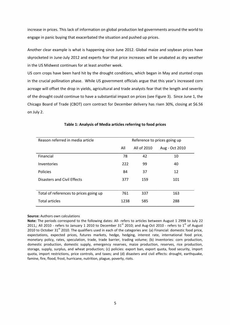
previous one – seemed to elicit a spike. The number of media articles on the price of wheat rose

significantly between August and October 2010, and 57 percent of the total number of media articles

with any reference to wheat prices reported that wheat prices were going to increase.

This number was 93 percentage points higher than the same measure in an average quarter for 2010

(see table 1).1

Among the major reasons for the price increases reported in the media were the fires in Russia (62

percent) and low inventories because of low production and stocks (25 percent), even though the

inventories and stocks were sufficient and significantly higher than in the 2008 crisis. Only 7 percent

of articles referred to policies, such as export bans, which had in fact been the major reason for the

1 To analyze all media articles, we use Sophic Intelligence Software, which is built on the Biomax BioXMä

Knowledge Management Suite. Each day, global food- and commodity-related news articles are loaded into Sophic Intel for linguistic analysis and semantic object network mapping. Sophic Intel generates wiki reports and heatmaps based on terms and phrases found in press articles that influence commodity price volatility and food security. The average quarter for 2010 has 122 articles where it is mentioned that wheat prices are increasing while the quarter from August to October 2010 has 210 articles, i.e. 72% higher.

Evidence: Based on the markets and their fundamentals

(Current and foreseeable supply, demand, stocks, trade, prices)

Perception: Media Reports on current and foreseeable supply,

demand, stocks, trade, prices

Prediction:

Price will go up

Prediction:

Price will go down

Evidence:

Price will go up

Evidence:

Price will stay

stable

Evidence:

Price will go down

Actual

Price

Combinations

Prediction:

Price will stay

stable

5

increase in prices. This lack of information on global production led governments around the world to

engage in panic buying that exacerbated the situation and pushed up prices.

Another clear example is what is happening since June 2012. Global maize and soybean prices have

skyrocketed in June-July 2012 and experts fear that price increases will be unabated as dry weather

in the US Midwest continues for at least another week.

US corn crops have been hard hit by the drought conditions, which began in May and stunted crops

in the crucial pollination phase. While US government officials argue that this year’s increased corn

acreage will offset the drop in yields, agricultural and trade analysts fear that the length and severity

of the drought could continue to have a substantial impact on prices (see Figure 3). Since June 1, the

Chicago Board of Trade (CBOT) corn contract for December delivery has risen 30%, closing at $6.56

on July 2.

Table 1: Analysis of Media articles referring to food prices

Reason referred in media article Reference to prices going up

All All of 2010 Aug - Oct 2010

Financial 78 42 10

Inventories 222 99 40

Policies 84 37 12

Disasters and Civil Effects 377 159 101

Total of references to prices going up 761 337 163

Total articles 1238 585 288

Source: Authors own calculations Note: The periods correspond to the following dates: All- refers to articles between August 1 2998 to July 22 2011,; All 2010 - refers to January 1 2010 to December 31

st 2010; and Aug-Oct 2010 - refers to 1

st of August

2010 to October 31st

2010. The qualifiers used in each of the categories are: (a) Financial: domestic food price, expectations, expected prices, futures markets, hedge, hedging, interest rate, international food price, monetary policy, rates, speculation, trade, trade barrier, trading volume; (b) inventories: corn production, domestic production, domestic supply, emergency reserves, maize production, reserves, rice production, storage, supply, surplus, and wheat production; (c) policies: export ban, export quota, food security, import quota, import restrictions, price controls, and taxes; and (d) disasters and civil effects: drought, earthquake, famine, fire, flood, frost, hurricane, nutrition, plague, poverty, riots.

6

Figure 3: Weekly Global Maize and Soybean Prices, June 2012

Soybean prices have experienced similarly sharp spikes, seeing their highest levels in nearly four

years (see Figure 3). The jump in prices has been caused by a combination of dry weather

throughout the US and South America, decreased acreage in favor of more profitable corn, record

levels of Chinese imports, and a subsequent rapid rate of stock disappearance. A June USDA report

cites soybean disappearance of 707 million bushels in May, the second largest on record. Increased

Chinese imports are being driven by strong demand from the Chinese crushing industry, reduced

domestic soybean production, and stockpiling of soybeans to guard against any potential shortage

resulting from US and Argentine droughts. Since June 1, CBOT soybean contracts for September

have risen 14%, closing at $14.52 on July 2.

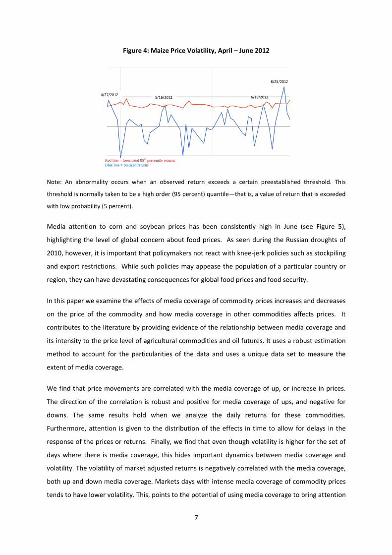
Although, the Maize Excessive Food Price Volatility (according to a measure of price volatility recently

developed at IFPRI2) have not yet shown significantly higher volatility, Soybeans by July 7th is already

in levels above normal (moderate volatility3). In both cases realized returns have been above the

forecasted 95th percentile returns in several instances, particularly in the case of maize (see Figure 4).

2 C. Martins-Filho, M. Torero, and F. Yao, “Estimation of Quantiles Based on Nonlinear Models of Commodity

Price Dynamics and Extreme Value Theory” (Washington, DC: International Food Policy Research Institute, 2010), mimeo. Specifically A time period of excessive price volatility: A period of time characterized by extreme price variation (volatility) is a period of time in which we observe a large number of extreme positive returns. An extreme positive return is defined to be a return that exceeds a certain preestablished threshold. This threshold is normally taken to be a high order (95 or 99%) conditional quantile, (i.e. a value of return that is exceeded with low probability: 5 or 1%). In this model we are using the 95% quantile. 3 For further details see http://www.foodsecurityportal.org/soybean-price-volatility-alert-mechanism.

http://www.foodsecurityportal.org/soybean-price-volatility-alert-mechanism

7

Figure 4: Maize Price Volatility, April – June 2012

Note: An abnormality occurs when an observed return exceeds a certain preestablished threshold. This

threshold is normally taken to be a high order (95 percent) quantile—that is, a value of return that is exceeded

with low probability (5 percent).

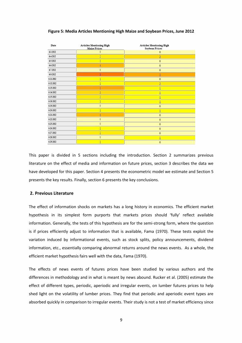
Media attention to corn and soybean prices has been consistently high in June (see Figure 5),

highlighting the level of global concern about food prices. As seen during the Russian droughts of

2010, however, it is important that policymakers not react with knee-jerk policies such as stockpiling

and export restrictions. While such policies may appease the population of a particular country or

region, they can have devastating consequences for global food prices and food security.

In this paper we examine the effects of media coverage of commodity prices increases and decreases

on the price of the commodity and how media coverage in other commodities affects prices. It

contributes to the literature by providing evidence of the relationship between media coverage and

its intensity to the price level of agricultural commodities and oil futures. It uses a robust estimation

method to account for the particularities of the data and uses a unique data set to measure the

extent of media coverage.

We find that price movements are correlated with the media coverage of up, or increase in prices.

The direction of the correlation is robust and positive for media coverage of ups, and negative for

downs. The same results hold when we analyze the daily returns for these commodities.

Furthermore, attention is given to the distribution of the effects in time to allow for delays in the

response of the prices or returns. Finally, we find that even though volatility is higher for the set of

days where there is media coverage, this hides important dynamics between media coverage and

volatility. The volatility of market adjusted returns is negatively correlated with the media coverage,

both up and down media coverage. Markets days with intense media coverage of commodity prices

tends to have lower volatility. This, points to the potential of using media coverage to bring attention

Red line = forecasted 95

th percentile returns

Blue line = realized returns

4/27/2012 5/16/2012 6/18/2012

6/25/2012

8

to the price surges and at the same time decrease volatility during food crises times or times when

there is above normal volatility.

In this paper we examine the effects of media coverage of commodity prices increases and decreases

on the price of the commodity and how media coverage in other commodities affects prices. It

contributes to the literature by providing evidence of the relationship between media coverage and

its intensity to the price level of agricultural commodities and oil futures. It uses a robust estimation

method to account for the particularities of the data and uses a unique data set to measure the

extent of media coverage.

We find that price movements are correlated with the media coverage of up, or increase in prices.

The direction of the correlation is robust and positive for media coverage of ups, and negative for

downs. The same results hold when we analyze the daily returns for these commodities.

Furthermore, attention is given to the distribution of the effects in time to allow for delays in the

response of the prices or returns. Finally, we find that even though volatility is higher for the set of

days where there is media coverage, this hides important dynamics between media coverage and

volatility. The volatility of market adjusted returns is negatively correlated with the media coverage,

both up and down media coverage. Markets days with intense media coverage of commodity prices

tends to have lower volatility. This, points to the potential of using media coverage to bring attention

to the price surges and at the same time decrease volatility during food crises times or times when

there is above normal volatility.

9

Figure 5: Media Articles Mentioning High Maize and Soybean Prices, June 2012

This paper is divided in 5 sections including the introduction. Section 2 summarizes previous

literature on the effect of media and information on future prices, section 3 describes the data we

have developed for this paper. Section 4 presents the econometric model we estimate and Section 5

presents the key results. Finally, section 6 presents the key conclusions.

2. Previous Literature

The effect of information shocks on markets has a long history in economics. The efficient market

hypothesis in its simplest form purports that markets prices should ‘fully’ reflect available

information. Generally, the tests of this hypothesis are for the semi-strong form, where the question

is if prices efficiently adjust to information that is available, Fama (1970). These tests exploit the

variation induced by informational events, such as stock splits, policy announcements, dividend

information, etc., essentially comparing abnormal returns around the news events. As a whole, the

efficient market hypothesis fairs well with the data, Fama (1970).

The effects of news events of futures prices have been studied by various authors and the

differences in methodology and in what is meant by news abound. Rucker et al. (2005) estimate the

effect of different types, periodic, aperiodic and irregular events, on lumber futures prices to help

shed light on the volatility of lumber prices. They find that periodic and aperiodic event types are

absorbed quickly in comparison to irregular events. Their study is not a test of market efficiency since

10

they do not exploit variation in timing of the news, but are interested in the structural aspects of the

response in markets to the types of events in the study.

Pruit(1987) studies the effects of the Chernobyl nuclear accident of the prices of agricultural futures

commodity prices produced in the Chernobyl area. He exploits the evolution of the news in the days

surrounding the accident and finds that the commodities studied experience an increase in volatility

that was short lived and that prices were affected as the efficient market hypothesis would predict.

Carter and Smith (2007) estimate the effect of news concerning the contamination of the corn supply

on the price of corn; they find that prices were affected and that the negative effect persisted for at

least a year.

Another vein of studies explores the effects of news on recalls and food safety on the prices of the

products. McKenzie and Thomsen (2001) find that red meat recalls due to contamination, food safety

information, negatively affects beef prices but that the transmission is not across all margins;

meaning, that farm level prices do not respond to this information. In a similar study, Schlenker and

Villas-Boas (2009) explore the effects of information on mad cow disease had on purchases and

futures prices. They find that future prices were negatively affected by the discovery of the first mad

cow and that information that is no “news”, in the sense that a talk show host just provided the

information available on mad cow disease thus just bringing attention to the issue, had half of the

effect of the event of effectively finding that mad cow disease was a problem in the meat supply.

Smith, van Ravenswaay and Thompson (1988) study the impact of contamination of milk on

consumer demand and find that media coverage had an impact on demand for milk, and that

negative media coverage had larger impacts. This studies show that media coverage can have large

impact on food prices, regardless of if the information is ‘news’ or just bringing attention to the

issues.

In the case of prices, media coverage of the price movement might be a signal of volatility in the

market. Given the extreme prices in food commodities that we observed during 2011, the issue of

what is the effect of media coverage on the price of these commodities is increasingly important.

News report of food price increase and decreases do not provide ‘new’ information to markets, as

these news articles are reporting the tendencies of the price series as they occur. However, as we

mentioned before, focusing attention in the dynamics of prices can serve as a signal of other

underlying issues or could reinforce the tendency by updating the beliefs not just of investor but also

consumers. Exaggerating the importance of price increases by the media or downplaying it can cause

welfare losses given that agents will make decisions based on information that does not reflect the

true nature of the pricing process.

11

3. Data

We use various data sources to estimate the impact of price movement media coverage on futures

markets. The first is daily futures price data from the Chicago Board of Trade for futures of Maize,

Soft, Soybean, Rice and Oil and from Kansas City Board of Trade for Hard Wheat. The future prices

selected are the closest to maturity each day. We augment these price data with market variables

such as the SP index, the daily exchange rates between the US dollar and the currencies of major

participant countries in the agricultural commodity markets, for example Canada, Thailand, China,

Australia, and The European Union.

The variables of interest for this paper are the measures of media coverage. Every day, we monitor a

comprehensive set of RSS feeds4 drawn from global media outlets via Google news5. A total of 31

feeds related to global food prices and food security are monitored; these feeds include search

strings such as “food prices,” “food crisis,” “agricultural development,” “commodity prices,” “price of

maize,” “price of wheat,” “price of oil,” “price of rice,” “price of soybean,” etc. Stories are tagged

with a star if they are about: 1. global food security or food prices, 2. ongoing national, regional, or

global food crises, 3. prices (international, regional, and national) or crop conditions of major

agricultural commodities (wheat, corn, soybeans, and rice), 4. oil prices, 5. Agricultural trade (export

bans, import or export forecasts, etc.), or 6. Agricultural/food policy research.

At the end of each day, all starred articles are converted into .txt files and saved using the format

“title_month_day_year.txt.” The day’s .txt files are then uploaded into the IFPRI Food Security

Analysis System, a tool built by Sophic Systems Alliance, called Sophic Intelligence Software. This

software, which is built on the Biomax BioXMä Knowledge Management Suite, uses linguistic and

semantic object network-mapping algorithms to analyze the relationships between key terms found

in each article. When articles are uploaded each day, the tool mines the complete database of

articles for a select set of key words. Sophic Intelligence Software generates a detail analysis of the

text within the articles and look at phrases in the articles that influence commodity price volatility

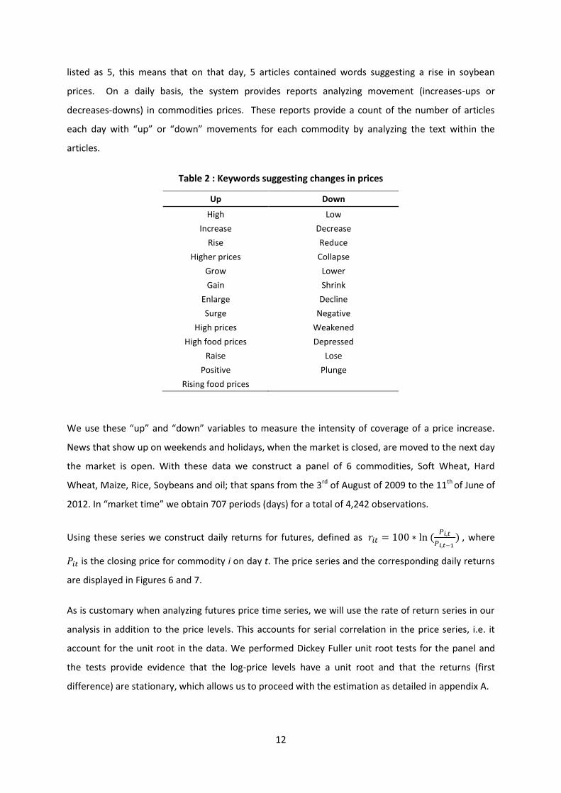
and food security. Table 2 lists the key words used to determine an “up” or “down” movement

within our data base of articles. For example, an article containing the words “soybean” and “surge”

would denote an “up” movement in soybean prices; if the soybean “up” report on a given day is

4 RSS stands for Really Simple Syndication. Also called web feeds, RSS is a content delivery vehicle. It is the

format used when you want to syndicate news and other web content. When it distributes the content it is called a feed. 5 The main sources of news are detailed in appendix B

12

listed as 5, this means that on that day, 5 articles contained words suggesting a rise in soybean

prices. On a daily basis, the system provides reports analyzing movement (increases-ups or

decreases-downs) in commodities prices. These reports provide a count of the number of articles

each day with “up” or “down” movements for each commodity by analyzing the text within the

articles.

Table 2 : Keywords suggesting changes in prices

Up Down

High Low

Increase Decrease

Rise Reduce

Higher prices Collapse

Grow Lower

Gain Shrink

Enlarge Decline

Surge Negative

High prices Weakened

High food prices Depressed

Raise Lose

Positive Plunge

Rising food prices

We use these “up” and “down” variables to measure the intensity of coverage of a price increase.

News that show up on weekends and holidays, when the market is closed, are moved to the next day

the market is open. With these data we construct a panel of 6 commodities, Soft Wheat, Hard

Wheat, Maize, Rice, Soybeans and oil; that spans from the 3rd of August of 2009 to the 11th of June of

2012. In “market time” we obtain 707 periods (days) for a total of 4,242 observations.

Using these series we construct daily returns for futures, defined as

, where

is the closing price for commodity i on day t. The price series and the corresponding daily returns

are displayed in Figures 6 and 7.

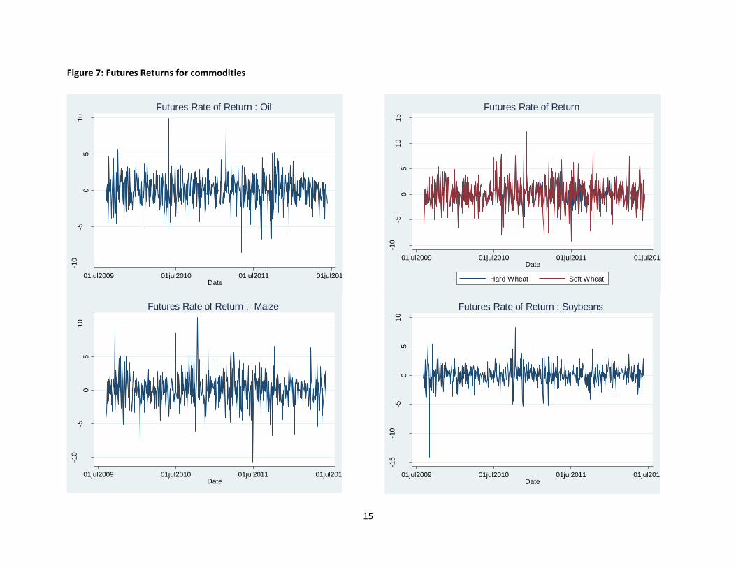
As is customary when analyzing futures price time series, we will use the rate of return series in our

analysis in addition to the price levels. This accounts for serial correlation in the price series, i.e. it

account for the unit root in the data. We performed Dickey Fuller unit root tests for the panel and

the tests provide evidence that the log-price levels have a unit root and that the returns (first

difference) are stationary, which allows us to proceed with the estimation as detailed in appendix A.

13

Table 3 and 4 shows the summary statistics for the variables used in the analysis. The price returns

are on average similar to other market variable returns. Across all commodities the average daily

return is 0.028% compared to a 0.038% return for the S&P index. We bring attention to the higher

volatility in commodities returns, as evidence by the larger standard error of the mean and the wider

ranges in comparison to the exchange rate returns and the S&P index. The largest negative return in

the sample is for soybean at -14.08% and the biggest gains in returns are for rice with 13.23% in a

day.

14

Figure 6: Futures Prices for commodities300

400

500

600

700

800

Pri

ce

01jul2009 01jul2010 01jul2011 01jul2012Date

Futures Price : Maize

60

80

100

120

Pri

ce


Futures Price : Oil

200

400

600

800

1000

Pri

ce


Hard Wheat Soft Wheat

Futures Price

800

1000

1200

1400

1600

Pri

ce


Futures Price : Soybeans

15

Figure 7: Futures Returns for commodities

-10

-50

510

Pri

ce R

etu

rns


Futures Rate of Return : Oil

-10

-50

510

Pri

ce R

etu

rns


Futures Rate of Return : Maize

-10

-50

510

15

Pri

ce R

etu

rns


Hard Wheat Soft Wheat

Futures Rate of Return

-15

-10

-50

510

Pri

ce R

etu

rns


Futures Rate of Return : Soybeans

16

Figure 8: Media Coverage of Price Changes, Ups and Downs

05

10

15


Increase in price news Decrease in price news

Price Changes News: Maize

02

46

8



Price Changes News: Soybeans

05

10

15

20

25



Price Changes News: Wheat

01

23

45



Price Changes News: Oil

17

We present the up and down variables used in the analysis for each commodity. The most activity in

news coverage is for Maize, Wheat and Rice. In table 3, we can corroborate the impressions from figure

8. Wheat and Rice have an average of just over 1 increase in price news per day, followed by Maize at

0.78 per day. For the decrease in price news, the activity is lower across the commodities, averaging

about 1 news article per 2 days related to a price decrease in Maize, Rice and Wheat and around 1 per 5

day period for soybeans and oil.

Table 3 : Summary Statistics

Mean SE Median Min Max Obs.

Hard Wheat

Price 248.23 1.99 252.43 168.38 363.03 707

Log-Price 5.491 0.008 5.53 5.13 5.89 707

Price Returns 0.017 0.081 -0.01 -8.00 8.66 706

Increase in price news 1.017 0.080 0 0 25 707

Decrease in price news 0.564 0.047 0 0 12 707

Maize

Price 536.70 5.44 586.75 306.25 786.00 707

Log-Price 6.246 0.011 6.37 5.72 6.67 707

Price Returns 0.071 0.080 0.00 -10.68 10.93 706



Oil

Price 87.13 0.44 85.19 64.78 113.39 707

Log-Price 4.459 0.005 4.44 4.17 4.73 707

Price Returns 0.020 0.074 0.06 -8.53 9.90 706



Rice

Price 14.00 0.06 14.07 9.43 18.39 707

Log-Price 2.632 0.005 2.64 2.24 2.91 707

Price Returns 0.004 0.067 -0.04 -5.41 13.23 706



Soft Wheat

Price 625.59 4.21 635.50 428.00 884.50 707

Log-Price 6.422 0.007 6.45 6.06 6.79 707

Price Returns 0.019 0.092 -0.07 -9.25 12.35 706



18

Table 4: Summary Statistics (continuation)

Soybeans

Price 1179.21 6.73 1201.50 885.00 1502.00 707

Log-Price 7.061 0.006 7.09 6.79 7.31 707

Price Returns 0.038 0.059 0.07 -14.08 8.34 706



Total

Log-Price 5.385 0.023 5.82 2.24 7.31 4242

Price Returns 0.028 0.031 0.00 -14.08 13.23 4236



Market Variables

Return SP Index 0.038 0.046 0.091 -6.896 4.632 706

Return Exchange rate- AU 0.023 0.032 0.032 -4.457 3.214 706

Return Exchange rate-EU -0.020 0.025 0.000 -2.046 2.385 706

Return Exchange rate-CND -0.005 0.025 -0.010 -2.131 3.368 706

Return Exchange rate- CHINA -0.010 0.004 -0.001 -0.573 0.621 706

Return Exchange rate- JP -0.026 0.023 -0.033 -2.230 3.002 706

Return Exchange rate- MX 0.009 0.027 -0.033 -2.528 3.708 706

Return Exchange rate- THAI -0.010 0.010 0.000 -1.127 1.043 706

Return T-bill 30 year rate -0.069 0.066 0.000 -8.611 7.612 706

4. Results

Next we present the results for our estimation. We estimates a model of futures price determination

that depends on the market conditions and the media coverage activity on the day the prices are

observed and or the market days immediately preceding the observation. Then we go on to estimate

the model to explore how the price volatility of the agricultural commodities and oil futures is affected

by the intensity of media attention in the days surrounding the price observation.

Price Levels

Our first estimates of the effects of media coverage are obtained by regressing the price levels on the

media variables while controlling for market conditions and the price level on the previous day. Changes

in future commodity prices due media coverage of price dynamics are shown in Table 5. In columns (1)–

(6), the dependent variable is the log of the price for each commodity.

19

Table 5 : Log Price Levels of Commodities

Log Price Levels of Commodities

OLS and Fixed Effects Estimates (1) (2) (3) (4) (5) (6)

Increase in price news -8.64 1.81 1.52 0.046 0.06 0.045

[1.89]*** [0.32]*** [0.22]*** [0.027]* [0.027]** [0.025]*

Decrease in price news 9.75 -0.37 -0.87 -0.075 -0.079 -0.08

[2.46]*** [0.49] [0.28]*** [0.045]* [0.045]* [0.040]**

Lag.Log-Price

1 0.99 0.99

[0.00018]*** [0.0028]*** [0.0032]***

Constant 540.6 705.9 673.3 0.012 4.61 8.14

[1.47]*** [1.01]*** [1.67]*** [0.098] [1.97]** [2.20]***

Commodity Effects No Yes Yes No Yes Yes

Market Controls No No Yes No No Yes

Observations 4242 4242 4236 4236 4236 4236

HAC-SE (in brackets) and Statistics robust to both arbitrary heteroskedasticity

and arbitrary common autocorrelation. Clustered on date. *<.10 **<.05 ***<.01

The baseline model is given in columns (1) to (3), where we include only the media coverage (increase

and decrease in price news) and we estimate via OLS, adding regressors from one column to the other.

Estimating the price level equation, omitting the commodity effects and the autocorrelation in the price

level we obtain, significant results and the signs of the coefficients imply that the media coverage

counteracts the trends in the commodity prices, meaning that increased reports of price spikes tend to

follow decreases in prices and vice versa. This specification implies that the appearance of one news

article reporting an increase in price is correlated with an 8.64% decrease in the price level, while for a

decrease in price media coverage the effect is an increase of 9.75%. Adding commodity specific fixed

effects in (2) flips the sign and implies a 1.8% increase in the price level per news article reporting price

increases and a 0.37% price decrease per article reporting a decrease in price. Adding the market

controls (3), change slightly the estimates, but the direction of the effects remains.

In columns (4) to (6) we run similar regressions but account for the autocorrelation in the future prices6.

The short run effects are very low, as expected. The estimates imply between 0.046% and 0.06%

increase in price of the commodity futures response per increased price news and between 0.075% and

0.08% decrease in price per decreased price news. The effect is only significant at the 10% level for the

decrease in price media coverage. The significant estimate for media coverage of price decreases in

6 See equation 1 in the appendix

20

column (6) implies a 0.08% decrease in the price level per decrease in price news article in the short run

and a 8% decrease in the ‘long’ run7. For the increase in price coverage, the estimates are around

0.045% and 4.5% in the short run and the long run respectively, and only significant at the 10% level.

In table 6, we present results for the distributed lag version of the model8. As before, we add regressors

sequentially from one column to the other. The estimates are in accord to the previous ones and reveal

that there is an split in the effect of the media coverage variable, with 0.056% decrease in the price due

to media coverage of price increases five days before (per article), and symmetric increase of 0.054% on

the day of the appearance of the news (per article). A parallel dynamic can be seen in the decrease in

price media coverage. From these estimates we can gather some of the dynamics between prices and

media coverage; news or media coverage of price increases tend to be followed with price increases, as

expected, but there is a dampening effect of price increases due to media coverage in the previous days,

meaning that prices tend to fall after increased media attention; the converse happens with media

coverage of price decreases. We reiterate that ‘long’ run effects can be obtained by multiplying the

short run effects discussed by 100, and that these effects on prices are economically meaningful9.

7 Note that since we are using daily data, the ‘long run’ is not necessarily a long time period. The long run

estimates in percentages are obtained by scaling the coefficient by the autocorrelation parameter i.e

as

defined in Eq. 1 in appendix A. Since the estimates is very close to one, we can approximate the effect by . 8 See equation 2 in the appendix

9 In addition, we note that more flexible specifications that allow for commodity specific trends and commodity

specific autocorrelation parameters were estimated and the results are qualitatively the same.

21

Table 6 : Log Price Levels of Commodities ADL Estimates

(1) (2) (3)

Lag-Log Price 1 0.99 0.99

[0.00020]*** [0.0027]*** [0.0033]***

Increase in price news 0.066 0.073 0.054

[0.022]*** [0.028]*** [0.026]**

Lag.Increase in price news 0.024 0.031 0.025

[0.024] [0.031] [0.029]

Lag2.Increase in price news -0.084 -0.077 -0.059

[0.024]*** [0.032]** [0.031]*

Lag3.Increase in price news -0.0023 0.0042 0.01

[0.022] [0.030] [0.028]


[0.021]* [0.026] [0.027]


[0.021]*** [0.028]* [0.027]**

Decrease in price news -0.091 -0.094 -0.09

[0.034]*** [0.045]** [0.041]**

Lag.Decrease in price news -0.012 -0.015 -0.01

[0.033] [0.045] [0.041]

Lag2.Decrease in price news 0.086 0.083 0.075

[0.031]*** [0.040]** [0.037]**


[0.032] [0.043] [0.038]


[0.033]** [0.042] [0.039]*


[0.030]* [0.039] [0.036]*

Constant 0.086 4.5 7.26

[0.12] [1.94]** [2.23]***

Commodity Effects No Yes Yes

Market Controls No No Yes

Observations 4212 4212 4212



22

Price Returns

We now turn to the discussion of the daily price returns equations10. In this estimates we use a methods

of moment procedure using as instruments the lagged differences of the media coverage variables of

each commodity.

The results for the estimation are presented in table 7. The direction of the effects remains unchanged

and the magnitudes are larger. From columns (1) to (3) we add the market controls and the commodity

fixed effects and note that the estimates are fairly robust to the inclusion of these variables. In column

(3) where commodity fixed effects and markets controls are included, the estimates imply a strong

relationship between media coverage and price returns. For every media article indicating ups the

returns increase by 0.135 percentage points and for articles indicating downs the returns decrease by

0.20 percentage points. In column (4) we estimate the distributed lag version of the equation and we

can see that the effects for media coverage of downs is potentially bigger as it is affected by the

previous days news, with up to 0.38 percentage point decrease for a 2 day period. In addition, the

dynamics mentioned are present but not precisely estimated; that is increase in prices news in the

previous days tend to counteract the price increase and vice versa.

In figure 9 we show the relative sizes of the effects we find in table 7 column (3). The total effect is the

part of the total variability in futures returns that is accounted by the up and down in the media and we

add what is accounted by the commodity effects or persistent commodity specific price shocks for

comparison.

First, the non-standardized effect shows that the size of the effect of the “Down” in media is comparable

to the effect of persistent commodity shocks, with just over 2% of the variation. The effect size for the

down variable is slightly lower.

In the second column we account only for the variability explained by the model, and compute similar

effects sizes. The difference in this column is that the variation in residuals is discarded; the implied

effects are very similar because much of the variation in returns is explained by the market variables.

Finally we compute the effect size discarding the residual variation and adjusting for the precision of the

estimates of each variable. These results are parallel to the results in table 7 but account directly for the

precision of the estimates and excludes the residual variation, but give us a clearer view of the effects.

10

Similar to equation1 in the appendix using the returns instead of the levels

23

The effects for increase in news media activity are larger than those for price decreases media activity,

and comparable to the effect of persistent commodity shocks. The increase in media activity account for

7.79% of the variation in return we observed in the data in comparison with 6.41% for the commodity

shock. The effect for decrease in price media activity is lower at 4.39%. These numbers can be

interpreted as the percent of the variability explained by the model that can be accounted for by each of

the media variables11. We note that in contrast with commodity shocks, the effects of the media are just

as important or more important in conjunction.

Table 7: Dependent Variable: Price Returns with Difference Instruments(DIV)

(1) (2) (3) (4)

UPS in price news 0.151 0.151 0.135 0.146

[0.059]** [0.059]** [0.054]** [0.071]**

DOWNS in price news -0.091 -0.091 -0.173 -0.204

[0.089] [0.089] [0.083]** [0.100]**

Lag.I UPS in price news

0.121

[0.074]

Lag2.UPS in price news

-0.121

[0.077]


-0.016

[0.062]

Lag.DOWNS in price news

-0.184

[0.088]**

Lag2.DOWNS in price news

0.107

[0.090]


-0.035

[0.086]

Commodity Effects No Yes Yes Yes

Market Controls No No Yes Yes

Observations 4212 4212 4212 4212

SE (in brackets) and Statistics robust to both arbitrary heteroskedasticity


The instruments are 5 lagged differences of media coverage for each commodity. In total there are 20

excluded instruments in the regressions.

11

The procedure used to obtain these numbers is analogous to partialling out the R2 in a regression framework.

24

Figure 9: Effect Size of Media Influence on Price Returns

Volatility

We explore changes in price volatility due to media coverage in two ways. First, we use simple F-test for

differences in the variance of prices on days where there are news and those where there is no news.

The question of whether the volatility of futures prices is different on days where there is media

coverage is of fundamental interest; namely, we want to know whether the volatility of the rate of

return on futures prices increases on days where there is media coverage indicating ups (positively

correlated) or downs (negative correlated). The second approach is a regression version of the first and

consists of estimating and equation of the conditional daily variance of returns, that is conditional on

market condition of the day12 that uses the squared residuals of the price level regressions discussed

before13.

We note that the ratio of the estimated variance of the rate of return (and the price level) on days with

news relative to no-news days,

is distributed as an F-statistic under the null hypothesis of equal

12

See equation 3 in appendix A 13

These residuals are essentially market adjusted returns.

2,23% 2,21%

6,41%

1,56% 1,55%

7,79%

2,10% 2,08%

4,39%

0,00%

2,00%

4,00%

6,00%

8,00%

10,00%

12,00%

14,00%

16,00%

18,00%

20,00%

Total effect %Effect Std. Effect

Effect Size of Media Influence on Price Returns

Down

Up

Commodity

25

variances. Table 9 shows the results of these tests for each type of coverage, namely days where there

are up news, down news and any type of news. The null hypothesis is that the ratio is equal to one, and

the alternatives are given in the column headers.

Table 9: Fisher Tests for difference in variances in price levels.

Obs Ha:Ratio<1 Ha:Ratio>1 Ha:Ratio!=1 F-Stat SD-No news SD- News

UPS-in price news 4242 0.003 0.997 0.005 0.879 1.454 1.551

Downs- in price news 4242 0.196 0.804 0.393 0.957 1.482 1.514

Any-News 4242 0.033 0.967 0.066 0.922 1.464 1.525

The tests in table 9 show that the volatility of price levels is not the same for the days where there are

news and the days where there are no news of changes in prices. For the days where there are up news

in comparison where there are no news or down news, there seems to be higher volatility for the days

with up news (p-value 0.003). The comparison between decreases in price news days and increases or

no news days yields no significant differences in volatility (p-value 0.393). Comparing the results for any

type of news, we can conclude that NO NEWS is better than NEWS in terms of price level volatility.

We conduct similar test for the futures price returns and present the results in table 10. The test

unequivocally point to higher variances/volatility on the days that there is media coverage.

Table 10: Fisher Tests for difference in variances in price returns

Obs Ha:Ratio<1 Ha:Ratio>1 Ha:Ratio!=1 F-Stat SD-No news SD- News

UPS- in price News 4236 0.000 1.000 0.000 0.805 1.947 2.170

DOWNS-in price News 4236 0.001 0.999 0.003 0.858 1.983 2.141

Any-News 4236 0.000 1.000 0.000 0.800 1.930 2.158

To further analyze volatility we present a graphical analysis of the squared residual of the market

adjusted model, given that this simple test might not reflect the heterogeneity in volatility due to the

intensity of media coverage. What we mean by this is that creating dichotomous groups that

agglomerate a day with one up news with a day with 10 up news might give the impression that media

coverage is positively correlated with volatility when it could also be the opposite. Figure 10 makes a

good case for this point.

26

The figures show that for days with fewer than 5 articles of up or down news, the residuals are very

spread out in comparison to ones in day with more than 5 articles. This evidence points to lower

volatility when media coverage is more intense.

Table 11 shows the estimations that put the graphs in a regression framework14. The message to take

away from these regression results is that volatility seems to be negatively correlated with the down

media coverage and these effects are lagged, i.e. the manifest themselves 1 and 2 days after the news

have appear. For the Up media coverage the regressions are not as conclusive. There is a significant

increase in volatility after the news has appeared, but this effect is overwhelmed by the negative effect

of days farther in the past. In summary, the evidence points to volatility being negatively correlated with

media coverage.

14

See equation 3 in appendix A

27

Figure 10: Squared Residual vs. Intensity of Media Coverage

0

.005

.01

.015

.02

Sq. R

esid

uals

0 5 10 15 20 25Increase in price news

Volatility : Residual Squared vs. Number of Up News

0

.005

.01

.015

.02

Sq. R

esid

uals

0 5 10 15Decrease in price news

Volatility : Residual Squared vs. Number of Down News

28

Table 11: Squared residuals (WITH controls) of Commodities Prices

OLS, Fixed Effects and ADL Estimates

(1) (2) (3) (4) (5) (6)

Lag.Sq. Residuals 0.084 0.069 0.064 0.084 0.069 0.063

[0.028]*** [0.027]*** [0.026]** [0.027]*** [0.026]*** [0.026]**

UPS in price news 0.089 0.02 -0.0048 0.052 0.018 0.0038

[0.073] [0.073] [0.072] [0.077] [0.075] [0.074]

DOWNS in price news 0.085 0.033 0.043 0.099 0.045 0.052

[0.13] [0.12] [0.12] [0.13] [0.13] [0.13]

Lag.I UPS in price news

0.29 0.26 0.24

[0.10]*** [0.10]** [0.098]**


-0.0047 -0.037 -0.045

[0.078] [0.079] [0.081]

Lag3. UPS in price news

0.12 0.08 0.034

[0.084] [0.084] [0.082]

Lag4. UPS in price news

-0.09 -0.12 -0.16

[0.084] [0.085] [0.085]*


0.031 -0.0029 -0.031

[0.077] [0.079] [0.083]

Lag. DOWNS in price news

-0.29 -0.34 -0.36

[0.14]** [0.14]** [0.13]***


-0.21 -0.27 -0.24

[0.094]** [0.094]*** [0.093]***


-0.094 -0.16 -0.099

[0.10] [0.10] [0.10]


0.18 0.12 0.17

[0.11] [0.11] [0.11]


-0.062 -0.12 -0.081

[0.098] [0.098] [0.098]

Commodity Effects No Yes Yes No Yes Yes

Market Controls No No Yes No No Yes

Observations 4230 4230 4230 4212 4212 4212



29

5. Conclusions

We have look at three important aspects of commodity markets, the price level, the returns these imply

and the volatility of these markets and relate them to coverage of those markets in the media. We

uncover interesting correlations between the price dynamics and the media coverage intensity.

The findings that more news report of up or downs in prices reinforce the price movement in the

direction of the report strengthen our case that increased media attention in some periods of food

crises can exacerbate the increase in price. We analyze the price level first, because this is what the poor

consumers of these commodities will feel. In addition, we highlighted the importance of thinking of the

dynamics between prices and media coverage; news or media coverage of price increases tend to be

followed with price increases, as mentioned, but there is a countervailing effect by the news activities of

the previous days. This is some evidence that media activity related to price increase puts some

downward pressure on the prices of the commodities when they are increasing.

We proceeded to analyze the returns because the behavior of investors and speculators are conditional

on them. We find similar conclusions for the returns equations. Returns also increase with media

coverage of increases in the price levels and decrease with the news of price decreases. In contrast to

the dynamics we found in the price level results, the effect of the media activity in the previous days is

only present for the decrease in prices media activity and tends to reinforce the downward pressure in

the returns.

The results for volatility show the importance of accounting by the intensity of media coverage and the

delayed response that can be expected, as by construction changes in volatility are only observed after

various changes in the price levels. Simple test of differences in variances hide the potential benefits

that increased media attention might have on the volatility of prices and returns. We find that the media

has good potential for reducing volatility. The variability of commodities returns and prices tends to

decrease as more attention is paid by the media to the situation in those commodities markets. This

stabilization force is present for both price increases and decreases reports by the media, but it is

stronger for decreases in prices media coverage.

30

6. References

Anderson, T. W. and C. Hsiao, 1981: “Estimation of Dynamic Models with Error Components”, Journal of the American Statistical Association, 76, 598-606.

Arellano, M. and O. Bover, 1995: “Another Look at the Instrumental-Variable Estimation of Error-Components Models”, Journal of Econometrics, 68, 29-51.

Arellano, M. and S. Bond, 1991: “Some Tests of Specification for Panel Data: Monte Carlo Evidence and an Application to Employment Equations”, Review of Economic Studies, 58, 277-297.

Blundell, R. and S. Bond, 1998: “Initial Conditions and Moment Restrictions in Dynamic Panel Data Models”, Journal of Econometrics, 87, 115-143.

Colin A Carter & Aaron Smith, 2007. "Estimating the Market Effect of a Food Scare: The Case of Genetically Modified StarLink Corn," The Review of Economics and Statistics, MIT Press, vol. 89(3), pages 522-533, 07.

Dubofsky, D. A., 1991, “Volatility Increases Subsequent to NYSE and AMEX Stock Splits,” Journal of Finance, 46, 421-431.

Fama, Eugene F., 1970, Efficient capital markets: A review of theory and empirical work, Journal of Finance 25, 383-417.

Han, Chirok & Phillips, Peter C. B., 2010. "Gmm Estimation For Dynamic Panels With Fixed Effects And Strong Instruments At Unity," Econometric Theory, Cambridge University Press, vol. 26(01), pages 119-151, February.

Mark E. Smith, Eileen O. van Ravenswaay and Stanley R. Thompson American Journal of Agricultural Economics Vol. 70, No. 3 (Aug., 1988), pp. 513-520

Martins-Filho, C., M. Torero, and F. Yao, “Estimation of Quantiles Based on Nonlinear Models of Commodity Price Dynamics and Extreme Value Theory” (Washington, DC: International Food Policy Research Institute, 2010), mimeo.

McKenzie, A.M., and M.R. Thomsen. "The Effect of E. Coli 0157:H7 on Beef Prices." Journal of Agricultural and Resource Economics 26(2001):431-44.

Nickell, S. (1981): “Biases in Dynamic Models with Fixed Effects”, Econometrica, 49, 1417-1426.

Ohlson, J. A., and S. H. Penman, 1985, “Volatility Increases Subsequent to Stock Splits: An Empirical Aberration,” Journal of Financial Economics, 14, 251-266.

Pruitt, S. W., Tawarangkoon, W. and Wei, K. C. J. (1987), Chernobyl, commodities, and chaos: An examination of the reaction of commodity futures prices to evolving information. J. Fut. Mark., 7: 555–569.

31

Randal R. Rucker & Walter N. Thurman & Jonathan K. Yoder, 2005. "Estimating the Structure of Market Reaction to News: Information Events and Lumber Futures Prices," American Journal of Agricultural Economics, Agricultural and Applied Economics Association, vol. 87(2), pages 482-500

Samuel B. Thompson, Simple formulas for standard errors that cluster by both firm and time, Journal of Financial Economics, Volume 99, Issue 1, January 2011, Pages 1-10

Wolfram Schlenker & Sofia B. Villas-Boas, 2009. "Consumer and Market Responses to Mad Cow Disease," American Journal of Agricultural Economics, Agricultural and Applied Economics Association, vol. 91(4), pages 1140-1152.

32

7. Appendix A : Econometric Model

To quantify the effect of media coverage of price increases and decrease on returns we use a market

model in that we control for market level variables, to focus on returns that are not explained by current

market conditions.

In our estimation we use 2 major frameworks. First the regression of price levels accounting for the

serial correlation in the prices. It is well known that fixed effects methods are not consistent with for

small N, Nickell (1981), and IV-GMM methods can be used to estimate these model [ Anderson and

Hsiao(1981) , Arellano and Bond (1991), Arellano and Bover (1995)].]. These methods suffer from weak

instrument problems which have been addressed by Blundell and Bond (1998) by proposing the further

moment restriction in the form of lag differences. We use insights from these methods to estimate the

impact of our media variables in inherently dynamic structure of the price data.

The equation we estimate is:

Eq. 1

Where

i = Hard Wheat, Maize, Oil, Rice, Soft Wheat, Soybeans

t = 1…T (1 is 08/03/2009 and T is 06/12/2012 in ‘market time’)

is the log price level

is a commodity specific intercept (fixed effect)

is the number of ‘increase in price of i news for day t

is the number of ‘decrease in price’ of i news for day t

is a matrix of market variables at date t

is a random error term, which depending of the specification will have a different structure

We assume that the news variables are predetermined or sequentially exogenous, that is that

which allow us to use moment restriction to obtain

a GMM-IV estimator. This equation might also contain lags of the regressors and/or additional lags of y,

but it captures the essential feature of the model that we want to estimate. Namely, a dynamic effect of

33

media coverage on the price level for which the speed of adjustment is governed by the coefficient of

lagged price level15.

The parameter we identify is the effect of changes in the appearance of news in the previous days of the

prices of commodities, i.e media coverage variation arising from differences in news coverage intensity

across commodities and time is essential source of exogenous variation.

We also explore the effects of news in the past five market days to see the short-lived but persistent

effects that the news data might reflect. Once price increase news appears, the likelihood that reports

of this price increase appear in the next days is higher. Thus the news data might have ‘runs,’ meaning

that we will see consecutive news reports followed by no news reports for a long period. We estimate a

distributed lag model parallel to the specification above to see if the ‘runs’ in news are also reflected in

the price (returns). In this case the equation for return becomes:

Eq. 2

Since we have a long panel time series dimension and a short panel variable, we use procedures that

required large T and include commodity fixed effects to account for persistent commodity shocks and

allow a flexible specification of the error terms to allow for persistent common shocks. Our procedures,

exploit the long time series aspect of the data, and allows for a flexible data generating process for the

error term allowing us to shed light into the price setting mechanism in commodities markets.

Finally, to explore the effects of media coverage on the price volatility we estimate the following model

(in addition to simple difference in variance tests); this is informed by the estimations in Ohlson and

Penman (1985) and Dubofsky (1991):

where

Eq. 3

15

To avoid issues of cointegration of commodity prices and exchange rates we use the return to the market (exchange) variables, which are stationary.

34

8. Appendix B: Details of Media Data and Sources

The measures of media coverage are obtained by monitoring a comprehensive set of for Really Simple

Syndication (RSS) feeds drawn from global media outlets via Google news. A non-exhaustive list of

sources of these feeds is:

Sources

ABC Fox Business Pakistan Daily Times

AFP Futures Magazine Politico

Agriculture.com Ghana News Agency Reuters

Agrimoney.com Hindu Business Line RTT News

All Africa Huffington Post San Francisco Chronicle

Arab News Independent Online The Australian

Associated Press of Pakistan Indian Express The Guardian

Barron's Inside Futures The Seattle Times

Bloomberg Kuwait Times Time Magazine

Business Day Los Angeles Times Times of India

Business Standard NASDAQ UK Telegraph

China Daily New York Times UN News Centre

CNBC Newstime Africa Wall Street Journal

Economic Times NPR Washington Post

Food World News Pakistan Business Recorder Weekly Times Now

A total of 31 feeds related to global food prices and food security are monitored; these feeds include

search strings such as :

Keywords AGOA Food security

Agricultural/food policy research Global food security

Agriculture development Import or export forecasts

Climate change National, regional, or global food crisis

Commodity Prices Oil world

Ethanol subsidies Price of maize or maize prices or maize export

Export bans Price of oil or oil prices or oil

FAO Price of rice or rice prices or rice export

Food crisis Price of soybean or soybean prices or soybean export or soyabean

Food prices Price of wheat or wheat prices or wheat export

ZEF-Discussion Papers on Development Policy No. 178

Documents

Transcript of ZEF-Discussion Papers on Development Policy No. 178