Youth Bulge, Civil Society, and Conflict Transformation

Shayna McCready sm8482a@american.edu

American UniversitySchool of International Service

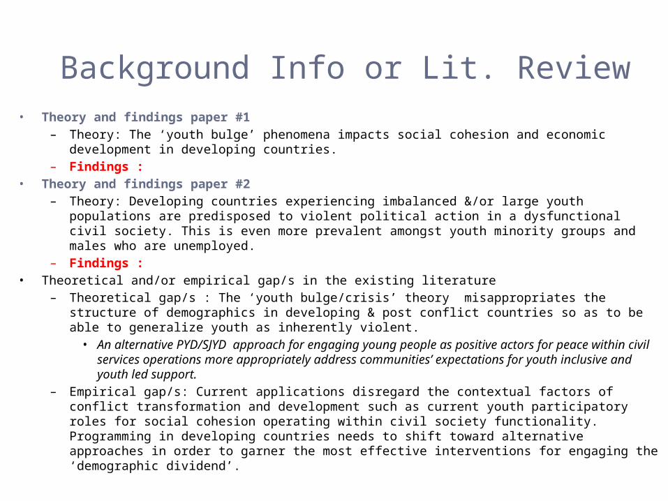
Background Info or Lit. Review• Theory and findings paper #1

– Theory: The ‘youth bulge’ phenomena impacts social cohesion and economic development in developing countries.

– Findings :• Theory and findings paper #2

– Theory: Developing countries experiencing imbalanced &/or large youth populations are predisposed to violent political action in a dysfunctional civil society. This is even more prevalent amongst youth minority groups and males who are unemployed.

– Findings :• Theoretical and/or empirical gap/s in the existing literature

– Theoretical gap/s : The ‘youth bulge/crisis’ theory misappropriates the structure of demographics in developing & post conflict countries so as to be able to generalize youth as inherently violent.

• An alternative PYD/SJYD approach for engaging young people as positive actors for peace within civil services operations more appropriately address communities’ expectations for youth inclusive and youth led support.

– Empirical gap/s: Current applications disregard the contextual factors of conflict transformation and development such as current youth participatory roles for social cohesion operating within civil society functionality. Programming in developing countries needs to shift toward alternative approaches in order to garner the most effective interventions for engaging the ‘demographic dividend’.

INTRO: Research Question & Hypothesis• Research Question(s) :

– Across countries experiencing booming youth populations, do individual perceptions of civil society impact social cohesion?

• What are the factors that drive confidence in the civil services?• Do those factors implicate justification for violent political actions?

• Research hypothesis/hypotheses:

– H0 =There is no relationship between individual perceptions of civil society and any of the factors that drive confidence in the civil services?

– H1 =Controlling for age, employment, social class, education, race, and gender, individual perceptions of civil society do impact social cohesion at the country level.

• Confidence in civil services will be highest amongst youthful minority groups who depend on them most • Justification of violence for political action will be lowest amongst those who have been positively

engaged by their community.

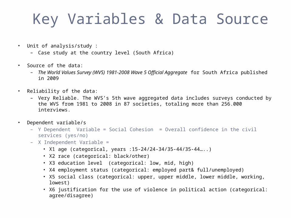
Key Variables & Data Source

• Unit of analysis/study : – Case study at the country level (South Africa)

• Source of the data: – The World Values Survey (WVS) 1981-2008 Wave 5 Official Aggregate for South Africa published in

2009

• Reliability of the data: – Very Reliable. The WVS’s 5th wave aggregated data includes surveys conducted by the WVS from

1981 to 2008 in 87 societies, totaling more than 256.000 interviews.

• Dependent variable/s– Y Dependent Variable = Social Cohesion = Overall confidence in the civil services (yes/no)– X Independent Variable =

• X1 age (categorical, years :15-24/24-34/35-44/35-44…..)• X2 race (categorical: black/other)• X3 education level (categorical: low, mid, high)• X4 employment status (categorical: employed part& full/unemployed)• X5 social class (categorical: upper, upper middle, lower middle, working, lowest)• X6 justification for the use of violence in political action (categorical: agree/disagree)

Descriptive Statistics Table or/and Graphics

mean 1.724963 2.474683 38.28894 3.115785 1.510507 38.28894 1.867916 3.643008 3.518588 stats e198 e069_08 x003 x007 x001 x003 x025r x028 x045

. tabstat e198 e069_08 x003 x007 x001 x003 x025r x028 x045

.

cv .5631012 .3582674 .5228404 .66652 .3236231 .3428103 max 4 4 6 8 3 5 min 1 1 1 1 1 1 iqr 1 1 2 5 1 3 p50 1 2 3 4 2 4 mean 1.724963 2.474683 2.864503 3.643008 1.867916 3.518588 N 2716 12284 11646 13216 11629 8527 stats e198 e069_08 x003r x028 x025r x045

. tabstat e198 e069_08 x003r x028 x025r x045, statistics(N mean median iqr min max cv)

13.88%

37.72%35.44%

12.95%

a great deal quite a lotnot very much none at all

Source: WVS

Confidence: the civil services

51.6%48.4%

yes no

Source: WVS

Confidence: the civil services

80.39%

19.61%

No Yes

Source: WVS

Unemployed, Yes=1

40.62%

59.38%

Other Black

Source: WVS

Race

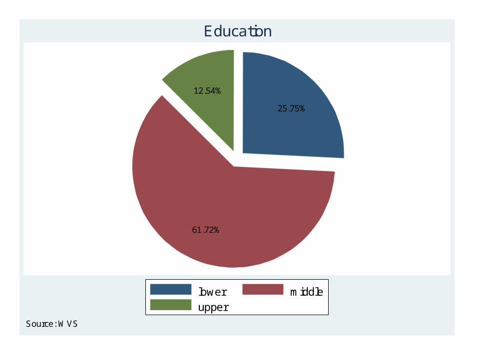
25.75%

61.72%

12.54%

lower middleupper

Source: WVS

Education

2.662%

23.96%

20.55%24.52%

28.31%

upper class upper middle classlower middle class working classlower class

Source: WVS

Social Class

22.03%

24.47%

21.89%

14.11%

11.62%

5.882%

15-24 25-3435-44 45-5455-64 65 and more years

Source: WVS

Age

Total 2,716 100.00 strongly disagree 242 8.91 100.00 disagree 284 10.46 91.09 agree 675 24.85 80.63 strongly agree 1,515 55.78 55.78 justified Freq. Percent Cum.political goals not using violence for

. tab e198

.

Total 12,284 100.00 none at all 1,591 12.95 100.00 not very much 4,354 35.44 87.05 quite a lot 4,634 37.72 51.60 a great deal 1,705 13.88 13.88 civil services Freq. Percent Cum. confidence: the

. tab e069_08

Total 11,629 100.00 upper 1,458 12.54 100.00 middle 7,177 61.72 87.46 lower 2,994 25.75 25.75 (recoded) Freq. Percent Cum. education level

. tab x025r

Total 8,527 100.00 lower class 2,414 28.31 100.00 working class 2,091 24.52 71.69 lower middle class 1,752 20.55 47.17 upper middle class 2,043 23.96 26.62 upper class 227 2.66 2.66 (subjective) Freq. Percent Cum. social class

. tab x045

.

Total 13,216 100.00 other 55 0.42 100.00 unemployed 2,592 19.61 99.58 students 1,490 11.27 79.97 housewife 1,350 10.21 68.70 retired 1,317 9.97 58.48 self employed 666 5.04 48.52 part time 860 6.51 43.48 full time 4,886 36.97 36.97 employment status Freq. Percent Cum.

. tab x028

.

Total 11,646 100.00 65 and more years 685 5.88 100.00 55-64 1,353 11.62 94.12 45-54 1,643 14.11 82.50 35-44 2,549 21.89 68.39 25-34 2,850 24.47 46.51 15-24 2,566 22.03 22.03 age recoded Freq. Percent Cum.

. tab x003r

gamma = 0.0036 ASE = 0.027 Pearson chi2(9) = 24.9615 Pr = 0.003

100.00 100.00 100.00 100.00 100.00 Total 394 933 829 345 2,501 10.91 8.47 7.36 9.57 8.64 strongly disagree 43 79 61 33 216 11.17 11.47 10.62 7.54 10.60 disagree 44 107 88 26 265 16.24 26.15 26.18 27.25 24.75 agree 64 244 217 94 619 61.68 53.91 55.85 55.65 56.02 strongly agree 243 503 463 192 1,401 justified a great d quite a l not very none at a Totalpolitical goals not confidence: the civil services using violence for

column percentage frequency Key

. tab e198 e069_08 , col chi gamma

gamma = 0.3090 ASE = 0.025 Pearson chi2(6) = 167.8350 Pr = 0.000

100.00 100.00 100.00 100.00 Total 824 847 678 2,349 9.10 10.51 20.65 12.94 none at all 75 89 140 304 32.04 34.24 49.41 37.85 not very much 264 290 335 889 40.05 41.68 24.93 36.27 quite a lot 330 353 169 852 18.81 13.58 5.01 12.94 a great deal 155 115 34 304 civil services low medium high Total confidence: the income level

column percentage frequency Key

. tab e069_08 x047r , col chi gamma

.

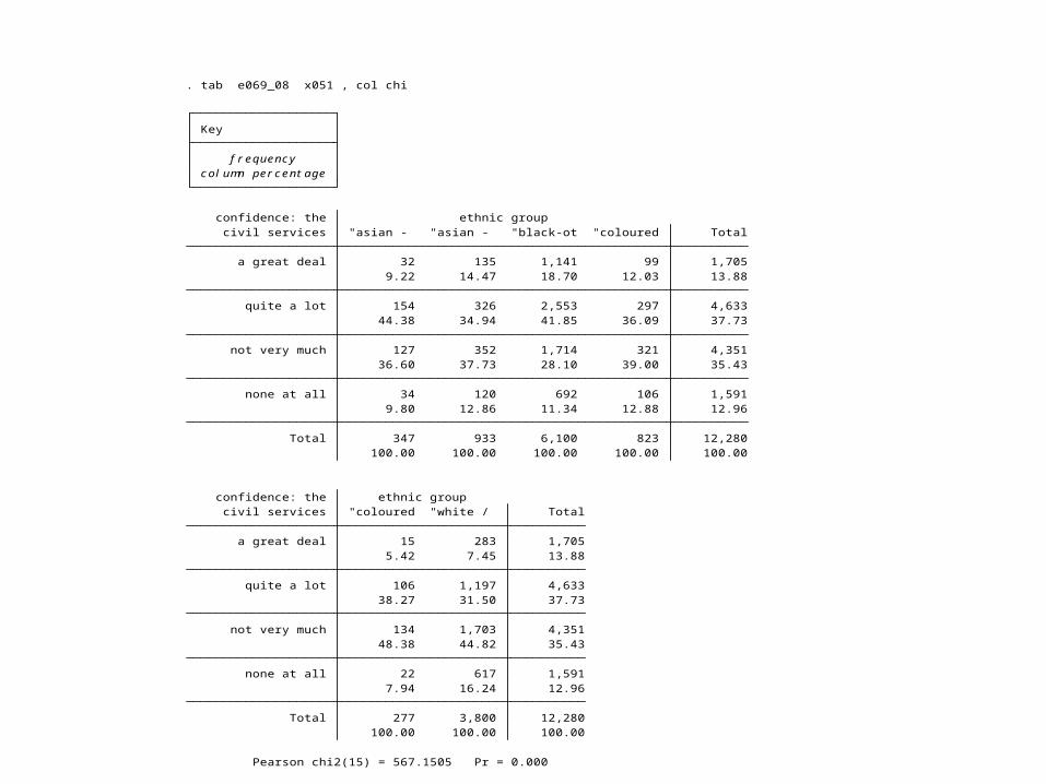
Pearson chi2(15) = 567.1505 Pr = 0.000

100.00 100.00 100.00 Total 277 3,800 12,280 7.94 16.24 12.96 none at all 22 617 1,591 48.38 44.82 35.43 not very much 134 1,703 4,351 38.27 31.50 37.73 quite a lot 106 1,197 4,633 5.42 7.45 13.88 a great deal 15 283 1,705 civil services "coloured "white / Total confidence: the ethnic group

100.00 100.00 100.00 100.00 100.00 Total 347 933 6,100 823 12,280 9.80 12.86 11.34 12.88 12.96 none at all 34 120 692 106 1,591 36.60 37.73 28.10 39.00 35.43 not very much 127 352 1,714 321 4,351 44.38 34.94 41.85 36.09 37.73 quite a lot 154 326 2,553 297 4,633 9.22 14.47 18.70 12.03 13.88 a great deal 32 135 1,141 99 1,705 civil services "asian - "asian - "black-ot "coloured Total confidence: the ethnic group

column percentage frequency Key

. tab e069_08 x051 , col chi

gamma = 0.2153 ASE = 0.014 Pearson chi2(6) = 266.7183 Pr = 0.000

100.00 100.00 100.00 100.00 Total 2,547 6,710 1,417 10,674 9.70 12.61 14.04 12.10 none at all 247 846 199 1,292 27.60 36.41 47.99 35.84 not very much 703 2,443 680 3,826 43.54 38.05 30.77 38.39 quite a lot 1,109 2,553 436 4,098 19.16 12.94 7.20 13.66 a great deal 488 868 102 1,458 civil services lower middle upper Total confidence: the education level (recoded)

column percentage frequency Key

. tab e069_08 x025r , col chi gamma

Bartlett's test for equal variances: chi2(3) = 1.3562 Prob>chi2 = 0.716

Total 2463236.49 10688 230.467486 Within groups 2453944.77 10685 229.66259Between groups 9291.7145 3 3097.23817 13.49 0.0000 Source SS df MS F Prob > F Analysis of Variance

Total 38.216391 15.181156 none at a 40.057276 15.427293 not very 38.763769 15.183776 quite a l 37.515587 15.103698 a great d 37.121918 14.976571 services Mean Std. Dev. the civil Summary of ageconfidence:

. oneway x003 e069_08, tabulate means standard

.

• Report Table with Gama/Lambda/Chi square statistic for association of ordinal/nominal data. • Report Table with T test/F test statistic for association of ordinal/nominal dependent variable and I-R

variables. • Interpretation of reported statistics in these tables:

– i) Does the association/ exists, i.e. is your measure of association/correlation statistically significant?– ii) If the association/correlation exists how strong it is? Check the value of the gamma or lambda

statistic;– iii) What is the direction of the association? Remember that this is for gamma statistic, for I_R and

ordinal LOM variables only. • Remember that chi square and lambda/gamma statistics may show ambiguous results, i.e. On of the measures

suggest associations and the other suggests no association.

Y - Gamma:

Y – Chi2: T/F tests Research hypothesis

education G= 0.2153 (0.0?)N = 10674

χ2= 266.7183(0.0?)N = 10674

t=? Reject the H0. Y and X1 are associated??????

income G=0.3090(0.0?), N = 2552

χ2=167.8350(0.?) N = 2552

t=? Fail to reject the H0. Y and X2 are not associated????

X3age

χ2=1.3562(0.?) N = 12280

t=? Mean of X3 for Y=0 is equal to Mean of X3 for Y=1 is equal to X3 has different means for are associated Y=0 and Y=1????

X4race

χ2=567.1505(0.?) N = 12280

?????

X5 Violence

G=0.0036(0.0?), N = 2501

χ2=24.9615(0.?) N = 2501

??????

unemployment

Regression Analysis, Probit Marginal Effects Estimates, The Dependent Variable is Confidence: the civil services, 0=Yes, 1= No

Interpretations:i)Does the association, i.e. is your coefficient statistically significant? Look this value. Is it <.05?

ii) If the association/correlation exists (sig <.05), what is the direction of the association/correlation, i.e. . What is the sign of the coefficient? iii) interpret the value of each and every statistically significant coefficient. For example, if the dependent and independent variables are not in log-level, and if b1=0.11, we can interpret this coefficients in the following way “one unit change in the independent variable X1 leads to 0.11 units changes in the dependent variables Y.” You can not interpret values of coefficients that are not significant since they are statistical zeros. iv) Make sure you interpret adj. R square statistics.

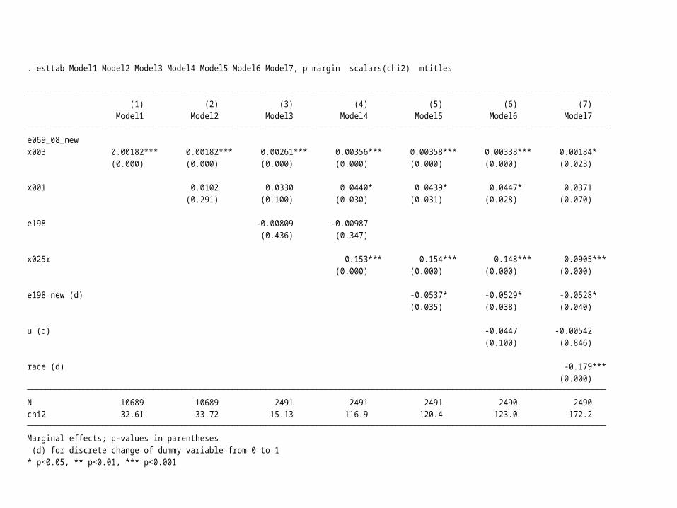
* p<0.05, ** p<0.01, *** p<0.001 (d) for discrete change of dummy variable from 0 to 1Marginal effects; p-values in parentheses chi2 32.61 33.72 15.13 116.9 120.4 123.0 172.2 N 10689 10689 2491 2491 2491 2490 2490 (0.000) race (d) -0.179***

(0.100) (0.846) u (d) -0.0447 -0.00542

(0.035) (0.038) (0.040) e198_new (d) -0.0537* -0.0529* -0.0528*

(0.000) (0.000) (0.000) (0.000) x025r 0.153*** 0.154*** 0.148*** 0.0905***

(0.436) (0.347) e198 -0.00809 -0.00987

(0.291) (0.100) (0.030) (0.031) (0.028) (0.070) x001 0.0102 0.0330 0.0440* 0.0439* 0.0447* 0.0371

(0.000) (0.000) (0.000) (0.000) (0.000) (0.000) (0.023) x003 0.00182*** 0.00182*** 0.00261*** 0.00356*** 0.00358*** 0.00338*** 0.00184* e069_08_new Model1 Model2 Model3 Model4 Model5 Model6 Model7 (1) (2) (3) (4) (5) (6) (7)

. esttab Model1 Model2 Model3 Model4 Model5 Model6 Model7, p margin scalars(chi2) mtitles

Findings & Policy Implications of the research

• Findings: Did you accept your research hypothesis?– Finding #1

– Finding #2

• What are the policy implications of your findings?