High performance numerical linear algebra:trends and new challenges.

Yousef SaadDepartment of Computer Science

and Engineering

University of Minnesota

HPC days in LyonApril 8, 2016

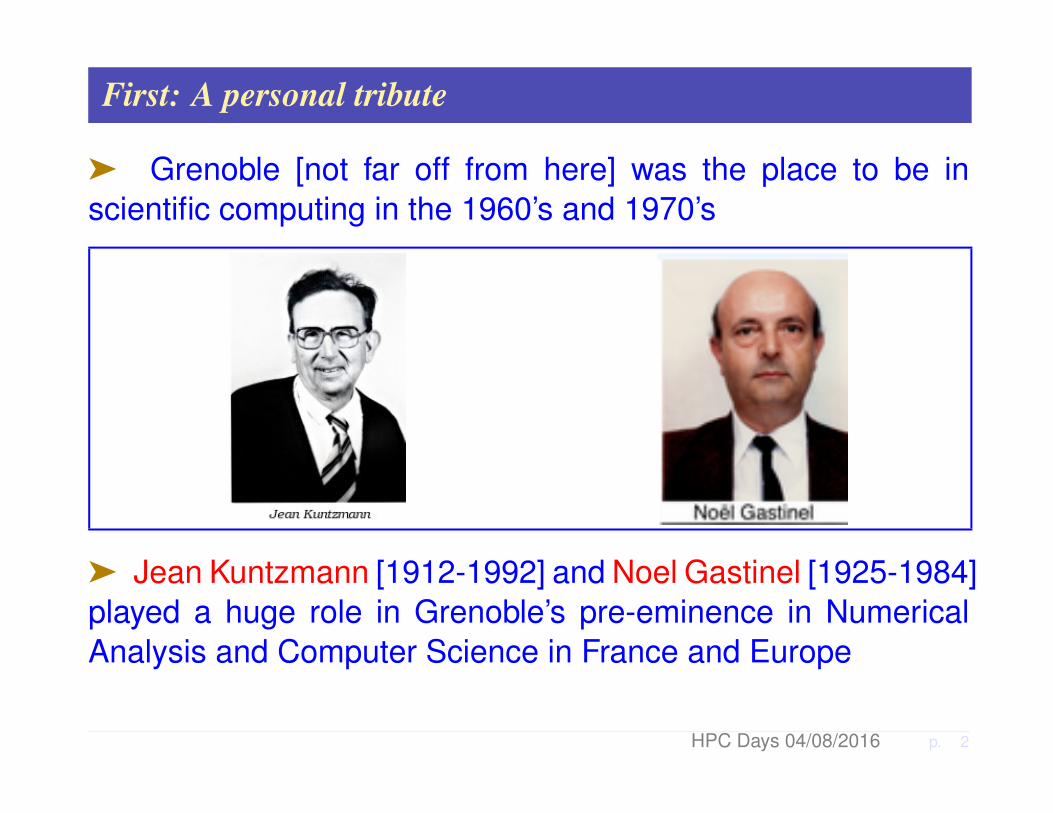
First: A personal tribute

ä Grenoble [not far off from here] was the place to be inscientific computing in the 1960’s and 1970’s

ä Jean Kuntzmann [1912-1992] and Noel Gastinel [1925-1984]played a huge role in Grenoble’s pre-eminence in NumericalAnalysis and Computer Science in France and Europe

HPC Days 04/08/2016 p. 2

Introduction: Numerical Linear Algebra

Numerical linear algebra has always been a “universal” tool inscience and engineering. Its focus has changed over the yearsto tackle “new challenges”

1940s–1950s: Major issue: the flutter problem in aerospaceengineering. Focus: eigenvalue problem.

ä Triggered discoveries of the LR and QR algorithms, and thepackage Eispack followed a little later

1960s: Problems related to the power grid promoted what weknow today as general sparse matrix techniques.

1970s: Finite Element methods, Computational Fluid Dynam-ics, reinforced need for general sparse techniques

HPC Days 04/08/2016 p. 3

Late 1980s – 1990s: Focus on parallel matrix computations.

Late 1990s: Big spur of interest in “financial computing” (Afterwhich the stock market collapsed ...)

ä Computational Mechanics (e.g., Fluid Dynamics, structures)has been a driving force in past few decades

ä But new forces are reshaping numerical linear algebra

Recent/Current: Google page rank, data mining, problemsrelated to internet technology, knowledge discovery, bio-informatics,nano-technology, ...

HPC Days 04/08/2016 p. 4

ä Major factor: Synergy between disciplines.

Example: Discoveries in materials (e.g. semi conductors re-placing vacuum tubes in 1950s) lead to faster computers, whichin turn lead to better physical simulations..

ä What about data-mining and materials?

ä Potential for a perfect union

ä A lot of recent interest

HPC Days 04/08/2016 p. 5

The plan:

1 The traditional: Sparse iterative solvers

– a brief tutorial

– recent research

2 The challenging: Materials science

– a brief tutorial

– solving very large eigenvalue problems

3 The new: Data Mining/ Machine learning

– a brief overview

– dimension reduction

HPC Days 04/08/2016 p. 6

PART 1: SPARSE ITERATIVE SOLVERS

Introduction: Linear System Solvers

General

Purpose

Specialized

Direct sparse Solvers

Iterative

A x = b∆ u = f− + bc

Methods Preconditioned Krylov

Fast PoissonSolvers

MultigridMethods

HPC Days 04/08/2016 p. 8

Long standing debate: direct vs. iterative

ä Starting in the 1970’s: huge progress of sparse direct solvers

ä Iterative methods - much older - not designed for ‘generalsystems’. Big push in the 1980s with help from ‘preconditioning’

ä General consensus now: Direct methods do well for 2-Dproblems and some specific applications [e.g., structures, ...]

ä Usually too expensive for 3-D problems

ä Huge difference between 2-D and 3-D case

ä Test: Two Laplacean matrices of same dimension n =122, 500. First: on a 350 × 350 grid (2D); Second: on a50× 50× 49 grid (3D)

HPC Days 04/08/2016 p. 9

ä Pattern of a similar [much smaller] coefficient matrix

0 100 200 300 400 500 600 700 800 900

0

100

200

300

400

500

600

700

800

900

nz = 4380

Finite Diff. Laplacean 30x30

0 100 200 300 400 500 600 700 800 900

0

100

200

300

400

500

600

700

800

900

nz = 5740

Finite Diff. Laplacean 10x10x9

HPC Days 04/08/2016 p. 10

A few observations

ä Problems are getting harder for Sparse Direct methods(more 3-D models, much bigger problems,..)

ä Problems are also getting difficult for iterative methodsCause: more complex models - away from Poisson

ä Researchers on both camps are learning each other’s tricksto develop preconditioners.

Current Challenges:

(1) Scalable (HPC) performance [for general systems]

(2) Robustness, general purpose preconditioners

HPC Days 04/08/2016 p. 11

Background: Preconditioned Krylov subspace methods

Two ingredients:

• An accelerator: Conjugate gradient, BiCG, GMRES,BICGSTAB,.. [‘Krylov subspace methods’]• A preconditioner: makes the system easier tosolve by accelator, e.g. Incomplete LU factorizations;SOR/SSOR; Multigrid, ...

One viewpoint:

ä Goal of preconditioner: generate good basic iterates.. [Gauss-Seidel, ILU, ...]

ä Goal of accelerator: find best combination of these iterates

HPC Days 04/08/2016 p. 12

Acceleration: Krylov subspace methods

ä Let x0 = initial guess, and r0 = b−Ax0 = initial residual

ä Define Km = spanr0, Ar0, · · · , Am−1r0 ...

ä ... Lm another subspace of dim. m

Basic Krylov step: seekxm = x0 + δ; δ ∈ Km such thatb−Axm ⊥ Lm

Projection method onKm orthogonally to Lm

ä Approximation theory viewpoint:

• xm = x0 + pm(A)r0 where pm = polynomial of deg. m−1

HPC Days 04/08/2016 p. 13

Two common and imporant choices

1. Lm = Km → class of Galerkin or orthogonal projectionmethods (e.g., Conjugate Gradient Method). WhenA is SPD:

‖x∗ − x‖A = minz∈K‖x∗ − z‖A.

2. Lm = AKm → class of minimal residual methods: CR,GCR, ORTHOMIN, GMRES, CGNR, .... xm satisfies:

‖b−Ax‖2 = minz∈K ‖b−Az‖2

ä Key to success of Krylov methods: Preconditioning

HPC Days 04/08/2016 p. 14

Preconditioning – Basic principles

Use Krylov subspace methodon a modified system, e.g.: M−1Ax = M−1b.

• The matrix M−1A need not be formed explicitly; only needto solve Mw = v whenever needed.

• Requirement : ‘easy’ to compute M−1v for arbitrary v

• Effect of preconditioner: spectrum of M−1A more favorablefor Krylov subspace accelerators

HPC Days 04/08/2016 p. 15

Both A and M are SPD: Preconditioned CG (PCG)

ALGORITHM : 1 Preconditioned Conjugate Gradient

1. Compute r0 := b−Ax0, z0 = M−1r0, and p0 := z0

2. For j = 0, 1, . . ., until convergence Do:3. αj := (rj, zj)/(Apj, pj)4. xj+1 := xj + αjpj5. rj+1 := rj − αjApj6. zj+1 := M−1rj+1

7. βj := (rj+1, zj+1)/(rj, zj)8. pj+1 := zj+1 + βjpj9. EndDo

ä Krylov method for M−1Ax = M−1b but use M -innerproduct to preserve self-adjointness.

HPC Days 04/08/2016 p. 16

Background: Incomplete LU (ILU) preconditioners

ILU: A ≈ LU

Simplest Example: ILU(0) →

Common difficulties of ILUs:Often fail for indefinite problemsNot too good for highly parallel environments

HPC Days 04/08/2016 p. 17

Sparse matrix computations with GPUs ∗∗

ä Very popular approach to: inexpensive supercomputing

ä Can buy∼ one Teraflop peak power for around $1,000

Tesla C1060 240 cores; 930GF peak

ä Next: Fermi; followed by Kepler; thenMaxwell

ä Tesla K 80 : 2 × 2,496→ 4992 GPU cores. 24 GB Mem.;Peak: ≈ 2.91 TFLOPS double prec. [with clock Boost].

HPC Days 04/08/2016 p. 18

The CUDA environment: The big picture

ä A host (CPU) and an attached device (GPU)

Typical program:

1. Generate data on CPU2. Allocate memory on GPU

cudaMalloc(...)3. Send data Host→ GPU

cudaMemcpy(...)4. Execute GPU ‘kernel’:kernel <<<(...)>>>(..)5. Copy data GPU→CPU

cudaMemcpy(...) C P U

G P

U

HPC Days 04/08/2016 p. 19

Sparse matrix computations on GPUs

Main issue in using GPUs for sparse computations:

• Huge performance degradation due to ‘irregular sparsity’

ä Matrices:Matrix -name N NNZFEM/Cantilever 62,451 4,007,383Boeing/pwtk 217,918 11,634,424

ä Performance of Mat-Vecs on NVIDIA Tesla C1060

Single Precision Double PrecisionMatrix CSR JAD DIA+ CSR JAD DIA+

FEM/Cantilever 9.4 10.8 25.7 7.5 5.0 13.4Boeing/pwtk 8.9 16.6 29.5 7.2 10.4 14.5

HPC Days 04/08/2016 p. 20

ä More recent tests: NVIDIA M2070 (Fermi), Xeon X5675ä Double precision in Gflops

MATRIX Dim. N CPU CSR JAD HYB DIArma10 46,835 3.80 10.19 12.61 8.48 -cfd2 123,440 2.88 8.52 11.95 12.18 -majorbasis 160,000 2.92 4.81 11.70 11.54 13.06af_shell8 504,855 3.13 10.34 14.56 14.27 -lap7pt 1,000,000 2.59 4.66 11.58 12.44 18.70atmosmodd 1,270,432 2.09 4.69 10.89 10.97 16.03

ä CPU SpMV: Intel MKL, parallelized using OpenMPä HYB: from CUBLAS Library. [Uses ellpack+csr combination]

(*) Thanks: all matrices from the Univ. Florida sparse matrix collection

HPC Days 04/08/2016 p. 21

Sparse Forward/Backward Sweeps

ä Next major ingredient of precond. Krylov subs. methods

ä ILU preconditioningoperations require L/Usolves: x← U−1L−1xä Sequential outer loop.

for i=1:nfor j=ia(i):ia(i+1)

x(i) = x(i) - a(j)*x(ja(j))end

end

ä Parallelism can be achieved with level scheduling:

• Group unknowns into levels

• Compute unknowns x(i) of same level simultaneously

• 1 ≤ nlev ≤ n

HPC Days 04/08/2016 p. 22

ILU: Sparse Forward/Backward Sweeps

• Very poor performance [relative to CPU]

Matrix NCPU GPU-Lev

Mflops #lev MflopsBoeing/bcsstk36 23,052 627 4,457 43FEM/Cantilever 62,451 653 2,397 168COP/CASEYK 696,665 394 273 142COP/CASEKU 208,340 373 272 115

Pre

c:m

iser

able

:-)

GPU Sparse Triangular Solve with Level Scheduling

ä Very poor performance when #levs is large

ä A few things can be done to reduce the # levels but perf. willremain poor

HPC Days 04/08/2016 p. 23

So...

... prepare for the demise of the GPUs...

... or the demise of the ILUs ?

HPC Days 04/08/2016 p. 24

Alternative: Low-rank approximation preconditioners

• Goal: use standardDomain Decompositionframework• Exploit Low-rank correc-tions• Consider a domain par-titioned in p sub-domainsusing vertex- based parti-tioniong (edge-separator)ä Interface nodes in eachdomain are listed last. 32 4 5

7 8 9 10

11 12 13 15

17 18

21 22 23 24 25

201916

6

1

14

HPC Days 04/08/2016 p. 25

The global system: Global view

ä Global system can bepermuted to the form→ä ui’s internal variablesä y interface variables

External interface points

Interior points

pointsLocal interface

B1 . . . F1

B2 . . . F2... . . . ...

Bp FpET

1 ET2 . . . ET

p C

u1

u2...upy

= b

ä Fi maps local interface points tointerior points in domain Ωi

ä ETi does the reverse operation

HPC Days 04/08/2016 p. 26

Example:

0 100 200 300 400 500 600 700 800 900

0

100

200

300

400

500

600

700

800

900

nz = 4380

HPC Days 04/08/2016 p. 27

Splitting

ä Split as: A ≡(B F

ET C

)=

(BC

)+

(F

ET

)

ä Define: F ≡(F−I

); E ≡

(E−I

)Then:[

B F

ET C

]=

[B + F ET 0

0 C + I

]− FET .

ä Property: F ET is ’lo-cal’, i.e., no inter-domaincouplings→

A0 ≡[B + F ET 0

0 C + I

]= block-diagonal

HPC Days 04/08/2016 p. 28

Low-Rank Approximation DD preconditioners

Sherman-Morrison→ A−1 = A−10 +A−1

0 FG−1ETA−10

G ≡ I − ETA−10 F

Options: (a) Approximate A−10 F,ETA−1

0 , G−1

(b) Approximate only G−1 [this talk]

ä (b) requires 2 solves with A0.

Let G ≈ Gk

Preconditioner→M−1 = A−1

0 +A−10 FG−1

k ETA−1

0

HPC Days 04/08/2016 p. 29

Symmetric Positive Definite case

ä Recap: Let G ≡ I − ETA−10 E ≡ I −H . Then

A−1 = A−10 +A−1

0 EG−1ETA−10

ä Approximate G−1 by G−1k → preconditioner:

M−1 = A−10 + (A−1

0 E)G−1k (ETA−1

0 )

ä Matrix A0 is SPD

ä Can show: 0 ≤ λj(H) < 1 .

HPC Days 04/08/2016 p. 30

ä Now take rank-k approximation to H :H ≈ UkDkU

Tk Gk = I − UkDkU

Tk →

G−1k ≡ (I − UkDkU

Tk )−1 = I + Uk[(I −Dk)

−1 − I]UTk

ä Observation: A−1 = M−1 +A−10 E[G−1 −G−1

k ]ETA−10

ä Gk: k largest eigenvalues of H matched – others set == 0

ä Result: AM−1 has• n− s+ k eigenvalues == 1• All others between 0 and 1

HPC Days 04/08/2016 p. 31

Alternative: reset lowest eigenvalues to constant

ä Let H = UΛUT = exact (full) diagonalization of H

ä We replaced Λ by:

λ1

λ2. . .

λk0

. . .0

ä Alternative: replace Λ by

λ1

λ2. . .

λkθ

. . .θ

ä Interesting case: θ = λk+1

ä Question: related approximation to G−1?

HPC Days 04/08/2016 p. 32

ä Result: Let γ = 1/(1− θ). Then approx. to G−1 is:

G−1k,θ ≡ γI + Uk[(I −Dk)

−1 − γI]UTk

ä Gk: k largest eigenvalues of G matched – others set == θ

ä θ = 0 yields previous case

ä When λk+1 ≤ θ < 1 we get

ä Result: AM−1 has• n− s+ k eigenvalues == 1• All others≥ 1

ä Next: An example for a 900 × 900 Laplacean, 4 domains,s = 119.

HPC Days 04/08/2016 p. 33

Eigenvalues of AM−1. Used: k = 5 . Two cases

θ = 0

0.1 0.2 0.3 0.4 0.5 0.6 0.7 0.8 0.9 1 1.1−2.5

−2

−1.5

−1

−0.5

0

0.5

1

1.5

2

2.5x 10

−12

θ = λk+1

0.5 1 1.5 2 2.5 3 3.5 4 4.5−4

−3

−2

−1

0

1

2

3

4x 10

−12

Proposition Assume θ is so that λk+1 ≤ θ < 1 . Then

the eigenvalues ηi of AM−1 satisfy:

1 ≤ ηi ≤ 1 +1

1− θ‖A1/2A−1

0 E‖22.

ä Can Show: For the Laplacean (FD)

‖A1/2A−10 E‖2

2 = ‖ETA−10 AA−1

0 E‖2 ≤1

4regardless of the mesh-size.

ä Best upper bound for θ = λk+1

ä Set θ = λk+1. Then κ(AM−1) ≤ constant, if k largeenough so that λk+1 ≤ constant.

ä i.e., need to capture sufficient part of spectrum

HPC Days 04/08/2016 p. 35

The symmetric indefinite case

ä Appeal of this approach over ILU: approximate inverse→Not as sensitive to indefiniteness

ä Part of the results shown still hold

ä But λi(H) can be > 1 now.

ä Can change the setting slightly [by introducing a parameterα] to improve diagonal dominance

ä Details skipped.

HPC Days 04/08/2016 p. 36

Parallel implementations

ä Recall : M−1 = A−10

[I + EG−1

k,θETA−1

0

]G−1k,θ = γI + Uk[(I −Dk)

−1 − γI]UTk

ä Steps involved in applying M−1 to a vector x :

ALGORITHM : 2 Preconditioning operation

1. z = A−10 x // Bi-solves andC∗ solve (C∗ ≡ C + I)

2. y = ETz // Interior points to interface (Loc.)3. yk = G−1

k,θy // Use Low-Rank approx.4. zk = Eyk // Interface to interior points (Loc.)5. u = A−1

0 (x+ zk) // Bi-solves andC∗- solve

HPC Days 04/08/2016 p. 37

A0 Solves Note:

A0 =

B1

B2. . .

Bp

C∗

ä Recall Bi = Bi + EiE

Ti

ä A solve with A0 amounts to all p Bi-solves and a C∗-solve

ä Can replace C−1∗ by a low degree polynomial [Chebyshev]

ä Can use any solver for the Bi’s

HPC Days 04/08/2016 p. 38

Parallel tests: Itasca (MSI)

ä HP linux cluster- with Xeon 5560 (“Nehalem”) processors

ä Simple Poisson equation on regular grid

2-D

Mesh Nproc Rank #its Prec-t Iter-t256× 256 2 8 29 2.30 .343512× 512 8 16 57 2.62 .747

1024× 1024 32 32 96 3.30 1.322048× 2048 128 64 154 4.84 2.38

3-D

Mesh Nproc Rank #its Prec-t Iter-t32× 32× 32 2 8 12 1.09 .097264× 64× 64 16 16 31 1.18 .381

128× 128× 128 128 32 62 2.42 .878

HPC Days 04/08/2016 p. 39

PART 2: ALGORITHMS FOR ELECTRONIC STRUCTURE

Approximations/theories used

ä Original Schrödinger equation very complex

ä Approximations developed started the 1930s reached ex-cellent level of accuracy. Among them...

Density Functional Theory: (DFT) observable quantities areuniquely determined by ground state charge density.

Kohn-Sham equation:

[−∇2

2+ Vion + VH + Vxc

]Ψ = EΨ

HPC Days 04/08/2016 p. 41

The three potential terms[−∇2

2+ Vion + VH + Vxc

]Ψ(r) = EΨ(r) With:

• Charge density: ρ(r) =∑occupi=1 |ψi(r)|2

• Hartree potential (local) ∇2VH = −4πρ(r)

• Vxc depends on func-tional. For LDA:

Vxc = f(ρ(r))

• Vion = nonlocal – doesnot explicitly depend on ρ

Vion = Vloc +∑aPa

ä Note: VH and Vxc depend nonlinearly on eigenvectors

HPC Days 04/08/2016 p. 42

Self Consistence

ä The potentials and/or charge densities must be self-consistent:Can be viewed as a nonlinear eigenvalue problem. Can besolved using different viewpoints

• Nonlinear eigenvalue problem: Linearize + iterate to self-consistence

• Nonlinear optimization: minimize energy [again linearize +achieve self-consistency]

The two viewpoints are more or less equivalent

ä Preferred approach: Broyden-type quasi-Newton technique

ä Typically, a small number of iterations are required

HPC Days 04/08/2016 p. 43

Self-Consistent Iteration

ä Most time-consuming part = computing eigenvalues / eigen-vectors.

Characteristic : Large number of eigenvalues /-vectors tocompute [occupied states].

ä Self-consistent loop takes a few iterations (say 10 or 20 ineasy cases).

Challenge: Compute a large number of eigenvalues (nev ≈104–105) of a large Hamiltonian matrix (N ≈ 107–108)

HPC Days 04/08/2016 p. 44

PARSEC

ä Represents≈ 15 years of effort bya multidisciplinary teamä Real-space Finite Difference;ä Efficient diagonalization, ...ä Exploits symmetry, ...ä PARSEC Released in∼ 2005.

HPC Days 04/08/2016 p. 45

DIAGONALIZATION: CHEBYSHEV FILTERING

Subspace iteration with Chebyshev filtering

Given a basis [v1, . . . , vm], ’filter’each vector as

vi = pk(A)vi

ä pk = Low deg. polynomial. Enhances wanted eigencompo-nents

The filtering step is not usedto compute eigenvectors ac-curately ä

SCF & diagonalization loopsmergedImportant: convergence stillgood and robust 0 0.5 1 1.5 2

−0.2

0

0.2

0.4

0.6

0.8

1

1.2

Deg. 6 Cheb. polynom., damped interv=[0.2, 2]

HPC Days 04/08/2016 p. 47

Main step:

Previous basis V = [v1, v2, · · · , vm]↓

Filter V = [p(A)v1, p(A)v2, · · · , p(A)vm]↓

Orthogonalize [V,R] = qr(V , 0)

ä The basis V is used to do a Ritz step (basis rotation)

C = V TAV → [U,D] = eig(C)→ V := V ∗ Uä Update charge density using this basis.

ä Update Hamiltonian — repeat

HPC Days 04/08/2016 p. 48

ä In effect: Nonlinear subspace iteration

ä Main advantages: (1) very inexpensive, (2) uses minimalstorage (m is a little≥ # states).

ä Filter polynomials: if [a, b] is interval to dampen, then

pk(t) =Ck(l(t))

Ck(l(c)); with l(t) =

2t− b− ab− a

• c ≈ eigenvalue farthest from (a+ b)/2 – used for scaling

ä 3-term recurrence of Chebyshev polynommial exploited tocompute pk(A)v. If B = l(A), then Ck+1(t) = 2tCk(t) −Ck−1(t)→

wk+1 = 2Bwk − wk−1

HPC Days 04/08/2016 p. 49

Tests with Silicon and Iron clusters (old)

Legend:

•nstate : number of states

•nH : size of Hamiltonian matrix

• # A ∗ x : number of total matrix-vector products

• # SCF : number of iteration steps to reach self-consistency

• total_eVatom

: total energy per atom in electron-volts

• 1st CPU : CPU time for the first step diagonalization

• total CPU : total CPU spent on diagonalizations

Reference: Y. Zhou, Y.S., M. L. Tiago, and J. R. Chelikowsky,Phy. Rev. E, vol. 74, p. 066704 (2006).

HPC Days 04/08/2016 p. 50

A comparison: Si525H276

method # A ∗ x SCF its. CPU(secs)ChebSI 124761 11 5946.69ARPACK 142047 10 62026.37TRLan 145909 10 26852.84

Polynomial degree = 8. Total energies agree to within 8 digits

A larger system: Si9041H1860

nstate # A ∗ x # SCF total_eVatom

1st CPU total CPU19015 4804488 18 -92.00412 102.12 h. 294.36 h.

# PEs = 48; nH =2,992,832. Pol. Deg. = 8.

HPC Days 04/08/2016 p. 51

Spectrum Slicing and the EVSL project

ä Part of our DOE project on excited states

Conceptually simple idea: cutthe overall interval containingthe spectrum into small sub-intervals and compute eigen-pairs in each sub-interval inde-pendently.Tool: polynomial filtering

−1 −0.8 −0.6 −0.4 −0.2 0 0.2 0.4 0.6 0.8 1−0.2

0

0.2

0.4

0.6

0.8

1

1.2

λφ

( λ )

ä To avoid repeting eigenpairs, keep only the computed eigen-values / vectors that are located in support interval

HPC Days 04/08/2016 p. 52

Levels of parallelism

Sli

ce

1S

lic

e 2

Sli

ce

3

Domain 1

Domain 2

Domain 3

Domain 4

Macro−task 1

The two main levels of parallelism in EVSL

HPC Days 04/08/2016 p. 53

Simple Parallelism: across intervals

ä Use OpenMP to illustrate scaling: Compute 1002 lowesteigenpairs of matrix SiO (n = 33, 401, nnz = 1, 317, 655.)

ä Use 4 and then 10 spec-tral slices

ä Near optimal scaling ob-served as # cores increases

ä Note: 2nd level of paral-lelism [re-orthogonalization+ MatVecs] not exploited.

0 2 4 6 8 10100

200

300

400

500

600

700

800

900

1000

1100Parallel scaling of the divide and conquer strategy

Number of OpenMP threads

Time(sec.)

4 intervals10 intervals

ä Faster solution times with 4 slices (≈ 250 evals per slice)than with 10 slices (≈ 100 evals per slice)

HPC Days 04/08/2016 p. 54

PART 3: DATA MINING

Introduction: a few factoids

ä Data is growing exponentially at an “alarming” rate:

• 90% of data in world today was created in last two years

• Every day, 2.3 Million terabytes (2.3×1018 bytes) created

ä Mixed blessing: Opportunities & big challenges.

ä Trend is re-shaping & energizing many research areas ...

ä ... including my own: numerical linear algebra

HPC Days 04/08/2016 p. 56

Introduction: What is data mining?

Set of methods and tools to extract meaningful informationor patterns from (big) datasets. Broad area : data analysis,machine learning, pattern recognition, information retrieval, ...

ä Tools used: linear algebra; Statistics; Graph theory; Approx-imation theory; Optimization; ...

ä This talk: brief introduction – emphasis on linear algebraviewpoint

ä + our initial work on materials.

ä Focus on “Dimension reduction methods”

HPC Days 04/08/2016 p. 57

Lots of data: can be hugely beneficial (e.g., Health sciences)

HPC Days 04/08/2016 p. 58

Major tool of Data Mining: Dimension reduction

ä Goal is not as much to reduce size (& cost) but to:

• Reduce noise and redundancy in data before performing atask [e.g., classification as in digit/face recognition]

• Discover important ‘features’ or ‘paramaters’

The problem: Given: X = [x1, · · · , xn] ∈ Rm×n, find a

low-dimens. representation Y = [y1, · · · , yn] ∈ Rd×n of X

ä Achieved by a mapping Φ : x ∈ Rm −→ y ∈ Rd so:

φ(xi) = yi, i = 1, · · · , n

HPC Days 04/08/2016 p. 59

m

n

X

Y

x

y

i

id

n

ä Φ may be linear : yi = W>xi , i.e., Y = W>X , ..

ä ... or nonlinear (implicit).

ä Mapping Φ required to: Preserve proximity? Maximizevariance? Preserve a certain graph?

HPC Days 04/08/2016 p. 60

Example: Principal Component Analysis (PCA)

In Principal Component Analysis W is computed to maxi-mize variance of projected data:

maxW∈Rm×d;W>W=I

n∑i=1

∥∥∥∥∥∥yi − 1

n

n∑j=1

yj

∥∥∥∥∥∥2

2

, yi = W>xi.

ä Leads to maximizing

Tr[W>(X − µe>)(X − µe>)>W

], µ = 1

nΣni=1xi

ä SolutionW = dominant eigenvectors of the covariancematrix≡ Set of left singular vectors of X = X − µe>

HPC Days 04/08/2016 p. 61

SVD:

X = UΣV >, U>U = I, V >V = I, Σ = Diag

ä Optimal W = Ud ≡ matrix of first d columns of U

ä Solution W also minimizes ‘reconstruction error’ ..

∑i

‖xi −WW Txi‖2 =∑i

‖xi −Wyi‖2

ä In some methods recentering to zero is not done, i.e., Xreplaced by X.

HPC Days 04/08/2016 p. 62

Unsupervised learning

“Unsupervised learning” : meth-ods that do not exploit known labelsä Example of digits: perform a 2-Dprojectionä Images of same digit tend tocluster (more or less)ä Such 2-D representations arepopular for visualizationä Can also try to find natural clus-ters in data, e.g., in materialsä Basic clusterning technique: K-means

−6 −4 −2 0 2 4 6 8−5

−4

−3

−2

−1

0

1

2

3

4

5PCA − digits : 5 −− 7

567

SuperhardPhotovoltaic

Superconductors

Catalytic

Ferromagnetic

Thermo−electricMulti−ferroics

HPC Days 04/08/2016 p. 63

Example: The ‘Swill-Roll’ (2000 points in 3-D)

−15 −10 −5 0 5 10 15−20

−10

0

10

20

−15

−10

−5

0

5

10

15

Original Data in 3−D

HPC Days 04/08/2016 p. 64

2-D ‘reductions’:

−20 −10 0 10 20−15

−10

−5

0

5

10

15PCA

−15 −10 −5 0 5 10−15

−10

−5

0

5

10

15LPP

Eigenmaps ONPP

HPC Days 04/08/2016 p. 65

Example: Digit images (a random sample of 30)

5 10 15

10

205 10 15

10

205 10 15

10

205 10 15

10

205 10 15

10

205 10 15

10

20

5 10 15

10

205 10 15

10

205 10 15

10

205 10 15

10

205 10 15

10

205 10 15

10

20

5 10 15

10

205 10 15

10

205 10 15

10

205 10 15

10

205 10 15

10

205 10 15

10

20

5 10 15

10

205 10 15

10

205 10 15

10

205 10 15

10

205 10 15

10

205 10 15

10

20

5 10 15

10

205 10 15

10

205 10 15

10

205 10 15

10

205 10 15

10

205 10 15

10

20

HPC Days 04/08/2016 p. 66

2-D ’reductions’:

−10 −5 0 5 10−6

−4

−2

0

2

4

6PCA − digits : 0 −− 4

01234

−0.2 −0.1 0 0.1 0.2−0.2

−0.15

−0.1

−0.05

0

0.05

0.1

0.15LLE − digits : 0 −− 4

0.07 0.071 0.072 0.073 0.074−0.15

−0.1

−0.05

0

0.05

0.1

0.15

0.2K−PCA − digits : 0 −− 4

01234

−5.4341 −5.4341 −5.4341 −5.4341 −5.4341

x 10−3

−0.25

−0.2

−0.15

−0.1

−0.05

0

0.05

0.1ONPP − digits : 0 −− 4

HPC Days 04/08/2016 p. 67

Supervised learning: classification

Problem: Given labels(say “A” and “B”) for eachitem of a given set, find amechanism to classify anunlabelled item into eitherthe “A” or the “B" class.

?

?ä Many applications.

ä Example: distinguish SPAM and non-SPAM messages

ä Can be extended to more than 2 classes.

HPC Days 04/08/2016 p. 68

Supervised learning: classification

ä Best illustration: written digits recognition example

Given: a set oflabeled samples(training set), andan (unlabeled) testimage.Problem: find

label of test image

Training data Test data

Dim

ensio

n red

uctio

n

Dig

it 0

Dig

fit

1

Dig

it 2

Dig

it 9

Dig

it ?

?

Dig

it 0

Dig

fit

1

Dig

it 2

Dig

it 9

Dig

it ?

?

ä Roughly speaking: we seek dimension reduction so thatrecognition is ‘more effective’ in low-dim. space

HPC Days 04/08/2016 p. 69

Supervised learning: Linear classification

Linear classifiers: Find a hy-perplane which best separatesthe data in classes A and B.

Linear

classifier

ä Note: The world in non-linear. Often this is combined withKernels – amounts to changing the inner product

HPC Days 04/08/2016 p. 70

Face Recognition – background

Problem: We are given a database of images: [arrays of pixelvalues]. And a test (new) image.

↑

?

Question: Does this new image correspond to one of thosein the database?

HPC Days 04/08/2016 p. 71

ä Techniques used in words:

“Build a (linear) projector that does well on some training data.Use that same projector to predict class of new item”

• Some methods use a graph - e.g., neighborhood graph

• Some methods use kernels (change inner products).

HPC Days 04/08/2016 p. 72

Example: Eigenfaces [Turk-Pentland, ’91]

ä Idea identical with the one we saw for digits:

– Consider each picture as a (1-D) column of all pixels– Put together into an arrayA of size #_pixels×#_images.

. . . =⇒ . . .

︸ ︷︷ ︸A

– Do an SVD ofA and perform comparison with any test imagein low-dim. space

– Similar to LSI in spirit – but data is not sparse.

HPC Days 04/08/2016 p. 73

Graph-based methods in a supervised setting

Test: ORL 40 subjects, 10 sample images each – sampleshown earlier # of pixels : 112× 92; TOT. # images : 400

10 20 30 40 50 60 70 80 90 1000.8

0.82

0.84

0.86

0.88

0.9

0.92

0.94

0.96

0.98ORL −− TrainPer−Class=5

onpppcaolpp−Rlaplacefisheronpp−Rolpp

HPC Days 04/08/2016 p. 74

ESTIMATING MATRIX RANKS

What dimension to use?

ä Important question – but a hard one.

ä Often, dimension k is selected in an ad-hoc way.

ä k = intrinsic rank of data.

ä Can we estimate it?

Two scenarios:

1. We know the magnitudeof the noise, say τ . Then,ignore any singular valuebelow τ and count the oth-ers.

2. We have no idea on themagnitude of noise. De-termine a good threshold τto use and count singularvalues > τ .

HPC Days 04/08/2016 p. 76

Use of Density of States [Lin-Lin, Chao Yang, YS]

ä Formally, the Density Of States (DOS) of a matrix A is

φ(t) =1

n

n∑j=1

δ(t− λj),

where• δ is the Dirac δ-function or Dirac distribution• λ1 ≤ λ2 ≤ · · · ≤ λn are the eigenvalues of A

ä Term used by mathematicians: Spectral Density

ä Note: number of eigenvalues in an interval [a, b] is

µ[a,b] =

∫ b

a

∑j

δ(t− λj) dt ≡∫ b

anφ(t)dt .

HPC Days 04/08/2016 p. 77

ä φ(t) == a probability distribution function == probability offinding eigenvalues of A in a given infinitesimal interval near t.

ä In Solid-State physics, λi’s represent single-particle energylevels.

ä So the DOS represents # of levels per unit energy.

ä Many uses in physics

HPC Days 04/08/2016 p. 78

The Kernel Polynomial Method

ä Used by Chemists to calculate the DOS – see Silver andRöder’94 , Wang ’94, Drabold-Sankey’93, + others

ä Basic idea: expand DOS into Chebyshev polynomials

ä Use trace estimators [discovered independently] to get tracesneeded in calculations

ä Assume change of variable done so eigenvalues lie in [−1, 1].

ä Include the weight function in the expansion so expand:

φ(t) =√

1− t2φ(t) =√

1− t2 ×1

n

n∑j=1

δ(t− λj).

Then, (full) expansion is: φ(t) =∑∞k=0µkTk(t).

HPC Days 04/08/2016 p. 79

ä Expansion coefficients µk are formally defined by:

µk =2− δk0

π

∫ 1

−1

1√

1− t2Tk(t)φ(t)dt

=2− δk0

π

∫ 1

−1

1√

1− t2Tk(t)

√1− t2φ(t)dt

=2− δk0

nπ

n∑j=1

Tk(λj).

ä Note:∑Tk(λi) = Tr [Tk(A)]

ä Estimate this, e.g., via stochastic estimator

ä Generate random vectors v(1), v(2), · · · , v(nvec) (normal dis-tribution, zero mean)

ä Some calculations similar to those of eigenvalue counts

HPC Days 04/08/2016 p. 80

An example with degree 80 polynomials

0 10 20 300

0.02

0.04

0.06

0.08

0.1

0.12

0.14

0.16

0.18

KPM, deg = 80

t

φ(t)

ExactKPM w/ Jackson

0 10 20 30

0

0.05

0.1

0.15

0.2

KPM, deg = 80

t

φ(t)

ExactKPM w/o Jackson

Left: Jackson damping; right: without Jackson damping.

HPC Days 04/08/2016 p. 81

Integrating to get eigenvalue counts

ä As already mentioned

µ[a,b] =

∫ b

a

∑j

δ(t− λj) dt ≡∫ b

anφ(t)dt

ä If we use KPM to approximate φ(t) = φ(t)/√

1− t2 then

µ[a,b] ≈m∑k=0

µk

∫ b

a

Tk(t)√1− t2

dt

ä A little calculation shows that the result obtained in this wayis identical with that of the eigenvalue count by Cheb expansion

HPC Days 04/08/2016 p. 82

Application: Estimating a threshold for rank estimation

ä When no other information is available, DOS can be usedto find a good cut-off value θ to use to estimate ranks

ä Common behavior:DOS decreases then in-creases (or stabilizes).ä If there is a significantgap use this to set-up θ.ä Often gives goodguess for cut-off between‘noise’ and ‘real’ sing.values 0 0.1 0.2 0.3 0.4 0.5 0.6 0.7 0.8 0.9 1

0

0.5

1

1.5

2

2.5

DOS with KPM, deg = 70

λ

φ (

λ )

HPC Days 04/08/2016 p. 83

Updating the partial SVD

ä In applications, data matrix X often updated

Challenge: Update the partial SVD as fast as possible [e.g.for ‘online’ applications..]

ä Example: Information Retrieval (IR), can add documents,add terms, change weights, ..

ä Methods based on projection techniques – developed in E.Vecharynski and YS’13. Details skipped

HPC Days 04/08/2016 p. 84

MATERIALS INFORMATICS

Data mining for materials: Materials Informatics

Definition: “The application of computational methodologiesto processing and interpreting scientific and engineering dataconcerning materials” [Editors. 2006 MRS bulletin issue onmaterials informatics]

ä Huge potential in exploiting two trends:

1 Improvements in efficiency and capabilities in computa-tional methods for materials

2 Recent progress in data mining techniques

ä Current practice: “One student, one alloy, one PhD” [seespecial MRS issue on materials informatics]→ Slow ..

ä Data Mining: can help speed-up process

HPC Days 04/08/2016 p. 86

Unsupervised learning

ä 1970s: Unsupervisedlearning “by hand”: Findcoordinates that will clus-ter materials according tostructureä 2-D projection fromphysical knowledgeä ‘Anomaly Detection’:helped find that compoundCu F does not exist

see: J. R. Chelikowsky, J. C. Phillips, Phys Rev. B 19 (1978).

HPC Days 04/08/2016 p. 87

Question: Can modern data mining achieve a similar dia-grammatic separation of structures?

ä Should use only information from the two constituent atoms

ä Experiment: 67 binary ‘octets’.

ä Use PCA – exploit only data from 2 constituent atoms:

1. Number of valence electrons;

2. Ionization energies of the s-states of the ion core;

3. Ionization energies of the p-states of the ion core;

4. Radii for the s-states as determined from model potentials;

5. Radii for the p-states as determined from model potentials.

HPC Days 04/08/2016 p. 88

ä Result:

−2 −1 0 1 2 3−2

−1.5

−1

−0.5

0

0.5

1

1.5

2

BN

SiC

MgS

ZnO

MgSe

CuCl

MgTe

CuBr

CuICdTe

AgI

ZWDRZWWR

HPC Days 04/08/2016 p. 89

Supervised learning: classification

Problem: classify an unknown binary compound into itscrystal structure class

ä 55 compounds, 6 crystal structure classesä “leave-one-out” experiment

Case 1: Use features 1:5 for atom A and 2:5 for atom B. Noscaling is applied.

Case 2: Features 2:5 from each atom + scale features 2 to 4by square root of # valence electrons (feature 1)

Case 3: Features 1:5 for atom A and 2:5 for atom B. Scalefeatures 2 and 3 by square root of # valence electrons.

HPC Days 04/08/2016 p. 90

Three methods tested

1. PCA classification. Project and do identification in space ofreduced dimension (Euclidean distance in low-dim space).

2. KNN K-nearest neighbor classification –

3. Orthogonal Neighborhood Preserving Projection (ONPP) - agraph based method - [see Kokiopoulou, YS, 2005]

Recognition rates for 3different methods usingdifferent features

Case KNN ONPP PCACase 1 0.909 0.945 0.945Case 2 0.945 0.945 1.000Case 3 0.945 0.945 0.982

HPC Days 04/08/2016 p. 91

Current work

ä Some data is becoming available

HPC Days 04/08/2016 p. 92

Current work

ä Huge recent increase of interest in the physics/chemstrycommunity

1. Predicting enthalpy of formation for a certain class of com-pounds.. [current]

2. Application to Orthophosphates of lanthanides (LnPO4)[current – with Edoardo di Napoli TRWH]

3. Project: Predict Band-gaps

HPC Days 04/08/2016 p. 93

Conclusion

ä Many, interesting new matrix problems in areas that involvethe effective mining of data

ä Among the most pressing issues is that of reducing compu-tational cost - [SVD, SDP, ..., too costly]

ä Many online resources available

ä Huge potential in areas like materials science though inertiahas to be overcome

ä On the + side: materials genome project is starting to ener-gize the field

ä To a researcher in computational linear algebra : big tide ofchange on types or problems, algorithms, HPC, culture,..

HPC Days 04/08/2016 p. 94

ä But change should be welcome

Two quotes:

“When one door closes, another opens; but weoften look so long and so regretfully upon theclosed door that we do not see the one which hasopened for us.

– Alexander Graham Bell

“Life is like riding a bicycle. To keep your balance,you must keep moving”

– Albert Einsten

HPC Days 04/08/2016 p. 95