You Owe Me*

Ulrike Malmendiera) and Klaus M. Schmidtb)

June 25, 2016

Abstract

In business and politics, gifts are often aimed at influencing the recipient at the ex-

pense of third parties. In an experimental study, which removes informational and

incentive confounds, subjects strongly respond to small gifts even though they un-

derstand the gift giver’s intention. Our findings question existing models of social

preferences. They point to anthropological and sociological theories about gifts cre-

ating an obligation to reciprocate. We capture these effects in a simple extension of

existing models. We show that common policy responses (disclosure, size limits)

may be ineffective, consistent with our model. Financial incentives are effective but

can backfire.

Keywords: Gift exchange; externalities; lobbyism; corruption; reciprocity; social

preferences.

JEL: C91, D62, D73, I11.

*) We would like to thank Yan Chen, Rachel Croson, Robert Dur, Ernst Fehr, Rudolf Kerschbamer, Matthias Kräkel,

George Loewenstein, Cristina Nistor. We would also like to thank seminar participants in the 2011 ASSA meetings,

the Third Behavioral Economics Annual Meeting (BEAM), and at the universities of Aix-Marseilles, Berkeley, Emory,

Innsbruck, Maastricht, MIT, Munich, Pennsylvania, Princeton, and Toulouse for comments and suggestions. David

Arnold, Leonie Giessing, Jana Jarecki, Sara Kwasnick, Eddie Ning, Warren Ronsiek, and Slobodan Sudaric provided

excellent research assistance. Financial support by Deutsche Forschungsgemeinschaft through SFB-TR 15, the Excel-

lence Initiative of the German government, and the Alfred P. Sloan Foundation is gratefully acknowledged. a) Ulrike Malmendier, Department of Economics, University of California at Berkeley, 501 Evans Hall, Berkeley, CA

94720-3880, USA, e-mail: ulrike@berkeley.edu b) Klaus M. Schmidt (corresponding author), Department of Economics, University of Munich, Ludwigstrasse 28, D-

80539 Munich, Germany, e-mail: klaus.schmidt@LMU.de

1 Introduction

Following Akerlof’s (1982) seminal paper on gift exchange in labor markets, a large experimental

literature has shown that gifts induce socially beneficial cooperation, both in the laboratory and in

the field (Fehr, Goette and Zehnder, 2009). Much less attention has been devoted to the ‘dark side’

of pro-social behavior: its negative externalities. Pro-social behavior towards one person may come

at the expense of a third party. Consider the wide-spread use of business gifts. In a typical scenario,

a procurement manager receives gifts (ranging from small tokens of appreciation, such as pens or

coffee mugs, to bottles of wine or event tickets) from a supplier, who hopes to get favorable treat-

ment. An extreme example is the pharmaceutical industry, estimated to spend $8-15k per year on

each physician in the US, including luxurious dinners, conferences at attractive locations, and gen-

erous honoraria (Blumenthal, 2004, p. 1885). Similarly, politicians and regulators receive gifts or

campaign contributions from lobbyists. In all cases the recipient makes a decision on behalf of a

third-party “client” who is often anonymous: shareholders, health insurances, or the electorate.

Such practices have raised concerns, and stirred a regulatory debate, about the influence of gifts.

Gift giving has been blamed as a major contributor to weak corporate governance, to the dramatic

rise of health care costs, and to wasteful pork barrel politics.1 Nevertheless, these externalities have

been largely ignored in the theoretical and experimental literature.

In this paper we use a controlled laboratory study to explore the negative externalities of

gift giving. First, we show that there is a powerful effect of the gift per se. Recipients reciprocate

to gifts even if there are no monetary incentives for doing so, the gift is small and does not convey

positive information about the gift giver or the product offered.2 Recipients fully understand that

the gift is given for selfish reasons, namely to influence their behavior at the expense of a third

party. We also observe a similar effect if a gift is expected, but not given: the decision-maker

discriminates against the potential gift giver. Second, we show that most standard models of social

preferences have difficulties predicting the observed behavior. It is better predicted by anthropo-

logical and sociological theories positing that gifts create an obligation to reciprocate. We propose

1 See e.g. Katz et al (2003), Blumenthal (2004), Susman (2008). Policy initiatives range from voluntary codes of

conduct (see e.g. Murphy [1995] on corporate ethics statements and Grande [2009] on self-regulation in the pharma-

ceutical industry) to regulatory reforms and laws limiting the possibilities for gifts and requiring disclosure, such as

the Lobbying Disclosure Act of 1995 and the Honest Leadership and Open Government Act of 2007 in the US. 2 In field settings, many gifts provide financial incentives or convey information. For example, physicians may pre-

scribe more drugs of a pharmaceutical company after attending a conference sponsored by that company because they

want to receive more sponsoring in the future or because of scientific information provided at the conference. These

effects are important and explained by standard economic theory. In this paper, we focus on the effects of a gift per se,

i.e., in the absence of any incentive or information effects.

2

a simple extension of standard models of social preferences that formalizes this idea. Third, we

conduct three policy treatments to evaluate the effectiveness of policy interventions that are often

proposed to mitigate the effects of gifts with negative externalities.

In our main treatment (Gift Treatment), a decision maker has to buy one of two possible

products on behalf of a client. Before making the decision, she may receive a small gift from one

of the two producers. The gift is given unconditionally and before the producers learn about the

value of their products, so that the gift cannot contain any information about the product’s quality.

The setting is anonymous, and players are re-matched after each round. Neither client nor producers

find out which product the decision maker picks, which excludes any reputation effects. Neverthe-

less, the effect of the gift is large. It is significantly stronger than in the classic gift-exchange game

without a third party, which we conducted in a control treatment (No Externality Treatment). Fur-

thermore, we observe that the gift is given with the intention to affect the decision of the recipient

at the expense of a third party. We show that the recipients are fully aware of this intention, but

they reciprocate nevertheless. We also find that, if a producer could have given a gift but chose not

to do so, the decision maker often punishes him by refusing to buy his product even if that product

is better. This punishment also comes at the expense of the client. Our results are robust to numer-

ous variations, including making gift giving more or less efficient, making the externalities on the

client very large, and giving the client a more active role by “hiring” the decision maker.

Our experimental design allows us to test whether decision makers are aware of how

strongly the gift affects their behavior. This question is much debated in practice. For example, a

questionnaire study by Steinman et al. (2001) found that only 39 percent of medical residents be-

lieve that gifts from pharmaceutical companies affect their own prescription behavior, but 84 per-

cent believe that other physicians are influenced. In our experiment, we asked decision makers at

the end to estimate how often their decisions coincided with the client’s preferences, and used a

quadratic scoring rule to induce unbiased estimates. On average, their estimates are highly accurate.

They somewhat overestimate by how much others are affected by the gift, but the estimated differ-

ence between own and others’ behavior is much smaller than in Steinman et al. (2001).

The most prominent economic theories of other-regarding behavior have difficulties pre-

dicting the observed phenomena. Theories of outcome-based social preferences such as altruism

(Andreoni and Miller, 2002), maximin preferences (Charness and Rabin, 2002), inequality aversion

(Fehr and Schmidt, 1999), and type-based reciprocity (Levine, 1998) are refuted by the observed

behavior. Theories of intention-based reciprocity (Rabin 1993, Dufwenberg and Kirchsteiger,

3

2004) have multiple equilibria including one in which no gift is given and the decision maker al-

ways chooses the best product for the client. Thus, they have little predictive power. Furthermore,

the underlying motives seem different. Producers admit in the questionnaire that they give the gift

for selfish reasons, and the decision makers state that they perfectly understand this.

Our evidence suggests that a gift triggers an obligation to repay, independently of the in-

tentions of the gift giver and the distributional consequences. It seems to create a bond between

gift giver and recipient, in line with a large anthropological and sociological literature on gifts

creating an obligation to reciprocate. In a classical study of small scale societies, Mauss (1924)

shows that reciprocity is the lubricant of social exchange and that people in these societies are

under an obligation to give and to reciprocate. Prominent sociologists such as Gouldner (1960) and

Blau (1964) argue that the obligation to reciprocate is a universal social norm.

We propose a simple theoretical framework that formalizes this idea. In the model the

weight that player i attaches to the welfare of player j depends on the actions of j that affect i,

relative to the expected behavior of j. A favorable act such as giving a gift strengthens the bond

between the giver and the recipient, i.e., the weight of the giver’s payoff in the recipient’s utility

function, and the recipient will reciprocate. The key difference to existing models of action-based

reciprocity (e.g., Cox et al., 2008) is the prediction that the more the favorable act exceeds expec-

tation, the stronger the positive response. We confirm this additional prediction in the data.

Finally, we conduct several policy treatments to evaluate remedies commonly proposed to

mitigate the problem of gift giving. In the Disclosure Treatment we inform clients which producer

gave the gift and which product the decision maker chose. Decision makers’ behavior remains very

similar to the Gift Treatment without disclosure. This holds even if clients can punish decision

makers (at a small cost to themselves) for choosing the wrong product.

Next, we address the effectiveness of size limits by varying the size of the gift. We find that

larger gifts have less of an impact. When the gift is three times as large, decision makers choose

the gift giver 22 percent less often than in the treatments where the gift is small. This is contrary to

the logic of size limits, and may be surprising at first glance; but it is predicted by our model:

decision makers correctly expect that producers will send the gift with a higher probability if it

benefits them more. The more the gift is expected, the smaller is the effect on behavior.

In a last policy treatment, the client can offer financial incentives to align the payoff of the

decision maker with his own interest. This is highly effective. When the client shares profits, the

effect of the gift is much less pronounced than in the Gift Treatment but still slightly stronger than

4

in the No Externality Treatment. However, when clients do not offer profit sharing (but could have

done so), the effect of the gift becomes even stronger than in the Gift Treatment. Again, these

results are consistent with the model we propose.

The rest of the paper is organized as follows: The next section discusses related literature.

Section 3 describes the experimental design. Section 4 shows that none of the most prominent

economic theories of social preferences predicts that the decision maker favors the gift giver. Sec-

tion 5 presents our main experimental results. We also analyze whether decision makers are aware

of how gifts affect their behavior. Section 6 offers a theoretical framework to explain the observed

behavior in terms of social preferences with endogenous reference groups. Section 7 considers the

policy treatments that test how to mitigate the effects of gift giving. Section 8 concludes.

2 Literature

In addition to the papers mentioned above (and the anthropological and sociological literature dis-

cussed in Section 6), our paper is related to three branches of the economics literature. First, a large

experimental literature, starting with Fehr, Kirchsteiger and Riedl (1993), has established reciproc-

ity as a motive for gift exchange. In almost all of the literature, the gift affects only the giver and

the receiver; there are no externalities. A notable exception is the “bribery game” in Abbink et al.

(2002) and Abbink (2004), where one player can bribe another player to take an action that is

beneficial to him at the expense of all other players in the experiment. The authors show that re-

peated interaction sustains a bribery relationship, but the threat of a (probabilistic) penalty and staff

rotation significantly weakens it. In contrast, we focus on the reciprocal effect of small gifts that

are given unconditionally without any repeated interaction, penalties, or monetary incentives.

A second related strand of the literature studies gifts with positive or negative externalities

in the field. Currie, Lin, and Meng (2013) conduct a field experiment in Chinese outpatient clinics,

where two trained auditors acting as patients visit a physician in sequence. If the first patient gives

a small gift to the physician, he receives better service and is less likely to be prescribed unneces-

sary and costly antibiotics than if no gift is given. Furthermore, if the first patient introduces the

second patient as his friend this patient also receives better service. Manacorda, Miguel and Vig-

orito (2011) estimate the impact of a large anti-poverty program in Uruguay on political support

for the government. Those (quasi-)randomly selected households that benefitted from the program

are 11-13 percentage points more likely to favor the government than those who did not benefit.

These studies show that reciprocity in the presence of externalities is not restricted to the lab but

5

extends to the field; however, they cannot identify the underlying behavioral mechanism.

Third, a large empirical literature studies business gifts, especially in the pharmaceutical

industry. In a meta-study of 29 data sets, Wazana (2000) concludes that gifts are “associated with

increased prescription rates of the sponsor’s medication” (p. 373). Campbell et al. (2007) conduct

a survey of 3,167 physicians in six specialties and document the types of gifts given by the phar-

maceutical industry and the nature of physician-industry interaction. Morgan et al. (2006) con-

ducted a survey among physicians on whether it is ethical to accept gifts of the pharmaceutical

industry and whether these gifts affect prescriptions. The general conclusion in this literature is that

business gifts are widespread and effective. However, as discussed in Dana and Loewenstein

(2003), the empirical literature cannot disentangle the causal factors that explain why gifts work.

3 Experimental Design

Our experimental design captures situations where one person has to rely on another person to

make a decision on his behalf, and a third party has an interest in influencing this decision. We

focus on the case where the latter party can give a small gift (such as a pen, coffee mug, or invitation

for lunch), the gift is given unconditionally, and the parties interact only once. Such small gifts are

common in many cultures and industries and, unlike bribes, are often legal and socially accepted.

In the experiment, two producers want to sell their products to a client. At the beginning of

each period one producer is chosen randomly as the potential gift giver. This producer receives one

additional token that he can pass on as a gift. The other producer cannot take any action. The

potential gift giver, called producer X, offers product X; the other producer, called producer Y,

offers product Y. The client has to buy either product X or product Y but has to rely on an expert to

make this decision on his behalf. We call the expert the decision maker (DM). DM receives a fixed

wage of 20 tokens for her services and is instructed to choose the best product for the client (“take

a decision that is in the best interest of the client.”) If she chooses product X (Y, respectively),

producer X (Y) receives a positive (quasi-)rent of 16 tokens, while the other producer gets 0. Before

DM decides producer X can pass the additional token on to her, in which case it doubles and DM

receives two tokens. The gift is unconditional, cannot be refused, and there is no repeated interac-

tion – subjects are anonymously re-matched after each round. The client is aware of the possibility

of a gift, but does not know whether a gift was actually given, nor which product was chosen.

6

A typical session has 24 subjects: 6 DMs, 6 clients, 6 producers X, and 6 producers Y.3

There are 20 periods. In each period DM is anonymously matched with a new client and new pro-

ducers X and Y. Products X and Y are simple 50/50 lotteries. The payoffs are natural numbers be-

tween 3 and 20. For example, product X may pay 5 or 11 with equal probability, while product Y

pays 3 or 17. The lottery pairs in each period are fixed throughout all treatments and sessions. In

four periods, the expected value of lottery X exceeds the expected value of Y by 2; in six periods,

the two lotteries have the same expected value (but differ in variance); in six periods, the expected

value of X is 2 points lower than the expected value of Y; and in four periods, the expected value

of X is 6 points lower. In this last case, product Y first-order stochastically dominates product X,

i.e., every rational decision maker (no matter how risk averse or risk loving) prefers Y to X. (There

are also three cases with an expected-payout difference of 2 where Y first-order stochastically

dominates. Appendix-Table A1 in Appendix B shows all 20 lottery pairs.)

Note that Producer X has to decide whether to send the gift before he learns what the prod-

ucts X and Y are in this period. Thus, the gift cannot signal product quality. The producers never

learn which product DM chooses. They are only informed about their total payoff after all 20 pe-

riods. Thus, there is no learning about the effectiveness of gifts, and a producer’s future behavior

cannot be affected by choosing or not choosing his product.

DM learns who the potential gift giver is and whether he sent the gift. She then sees the two

lotteries and chooses one for her client. Her payoff is unaffected by her choice, and she does not

learn how the lotteries resolve. The client does not know who the potential gift giver is and whether

he sends the gift. He sees the two products and is asked which one he would choose if, hypotheti-

cally, he could decide himself. He does not observe which product DM chooses, nor the outcome

of the lottery. At the end of the experiment he only learns the sum of his payoffs in all 20 periods.

In each session the instructions are read aloud. After 20 periods, subjects are asked to an-

swer a questionnaire. In the first part, DMs estimate how often their own decision and the decision

of the other DMs coincided with the preferred product of the clients. Similarly, clients and produc-

ers estimate how often the decision makers chose the product that the clients would have preferred.

The answers are incentivized with a quadratic scoring rule. In the second part, we ask subjects

about the motives for their own decisions and their beliefs about the motives of the other subjects.

We compare the results of this Gift Treatment (GT) to two other treatments, the Baseline

3 There is one session in the Incentive Treatment in which only 20 subjects participated (5 DMs, 5 clients, 10 produc-

ers). In the No Externality Treatments there are no clients, so in these sessions we had 8 DMs and 16 producers.

7

Treatment (BT) and the No Externality Treatment (NET). In both of these treatments, we use ex-

actly the same lotteries (“products”) in the same sequence as in the Gift Treatment.

In the Baseline Treatment producers cannot send a gift and gifts are never mentioned. This

treatment shows whether decision makers choose the products preferred by their clients if nobody

tries to influence them. Comparing BT and GT allows us to test both for the effect of gift giving

and for the effect of not giving a gift (despite having the option) relative to a world without gifts.

In the No Externality Treatment, there is no client and no fixed wage for the decision maker.

DM buys the product for herself and is full residual claimant of the lottery payoffs. This treatment

allows us to estimate to what extent the effect of gifts in the Gift Treatment reflects the fact that

DM acts on behalf of a third party and does not bear the consequences of her decisions.

We test the robustness of our results in several control treatments (discussed in Section 5.4).

Furthermore, we investigate three policy treatments: disclosure with and without punishment, var-

iation in gift size, and financial incentives (described in Section 7).

Discussion of Design Features. The experimental design has several features that merit discussion.

First, only one of the two producers can make a gift. Had we allowed both producers to offer gifts,

both producers would likely have done so in most periods, in which case we would have lost many

observations. Alternatively, we could allow both producers to also choose the size of their gifts and

to enter a rent-seeking tournament which may result in higher gifts. Or, we could vary the exter-

nalities of gifts for the other producer. These are interesting avenues for future research, and the

restriction to a non-competitive setting has to be kept in mind for the interpretation of our results.

Second, in the experiment the decision maker had no choice but to accept the gift. We chose

this experimental design to isolate the pure effect of the gift without further complications that arise

if the gift giver does not know whether his gift is accepted. In reality it is often difficult to refuse

the gift, but not impossible. Whether and when decision makers refuse to accept gifts that are in-

tended to influence their behavior are interesting questions for future research.

Third, the products are simple lotteries over monetary outcomes. This design feature gives

the decision maker some moral wiggle room: Even when product Y has a higher expected value

than product X, DM may justify buying X because it is less risky or because it gives a higher payoff

in one state of the world. Note, though, that our design includes cases in which every rational agent

prefers Y because it first-order stochastically dominates X. The Baseline Treatment will show that

subjects had no difficulties evaluating the simple lotteries. Also note that many real-world decisions

that motivate our study feature probabilistic consequences, such as the effects of a drug on a patient

8

or a policy measure on the general public.

Fourth, the client and the producers do not observe the decision of the decision maker but

learn only the sum of their payoffs over all 20 periods at the end of the experiment. We do not

impose this design feature for realism. Rather, we use it to make sure that reputation building or

learning cannot affect our results, but that it is the effect of the gift per se that we observe.

Experimental Procedures. We conducted 31 sessions with 20-24 participants in each session at

the MELESSA laboratory of the University of Munich in 2010, 2011, and 2015. Subjects were

undergraduate students of various disciplines from the University of Munich and the Technical

University of Munich.4 We involved 740 subjects, generating a data set of 4,140 observations.5

The vast majority (93%) of students were in the typical age range of 20-29, and slightly more than

half (54%) were women. Upon arrival at the lab subjects were randomly and anonymously assigned

to the different roles. Sessions lasted about one hour. On average, subjects earned €14 ($19.15),

which includes a show-up fee of €4 ($5.47). Further summary statistics are in Appendix-Table A2.

4 Behavioral Predictions

To guide our empirical analysis, we derive the predictions of existing theories of social preferences

for the response to (not) receiving a gift. Remember that the gift is given unconditionally and prior

to her decision. Thus, the traditional model of rational self-interested behavior does not predict that

DM favors the gift giver. She is indifferent between the two products, no matter whether the gift

was given. If there is no client and DM chooses the product for herself, the traditional model pre-

dicts that she chooses the better product. Thus, if we want to explain why the gift systematically

affects her decision, we have to look for alternative models.

First, we consider outcome-based social preferences, and in particular the three forms that

have received most interest in the literature: altruism, maximin preferences, and inequality aver-

sion. Suppose that DM has outcome-based social preferences UDM(mDM, mX, mY, mC), where im is

the expected monetary payoff of player i {DM, X, Y, C} and UDM is invariant to permutations of

(mX, mY, mC). Under (i) altruism in the form of utilitarianism (Andreoni and Miller, 2002) DM’s

utility increases with the sum of the payoffs of the others; under (ii) maximin preferences (Charness

and Rabin, 2002) DM’s utility increases with the payoff of the worst-off in the group; and under

4 We used the software ORSEE (Greiner 2004) for recruitment and z-Tree (Fischbacher 2007) for the experiments. 5 One additional session containing only 20 subjects (Disclosure Treatment) had to be excluded ex-post because of a

problem in the matching procedure in z-Tree. All results are robust to including this session.

9

(iii) inequality aversion (Fehr and Schmidt, 1999; Bolton and Ockenfels, 2000) DM dislikes to be

worse off and (to a lesser degree) to be better off than the other players.

We assume that the decision maker is risk neutral and evaluates products X and Y by their

expected values.6 We say that DM “favors” a producer if she chooses his product no matter how it

compares to the other product. We say that DM favors the client if she chooses the product with

the higher expected value or, if both have the same expected value, with the smaller variance. We

assume that if DM is indifferent she favors the client, as frequently imposed in contracting games

with multiple equilibria. This is confirmed by the results of the Baseline Treatment.

All outcome-based theories predict unambiguously that DMs should not be influenced by

gifts but should maximize the expected utility of their clients:

Proposition 1. Suppose that the decision maker is motivated by (i) altruism (utilitarianism), (ii)

maximin preferences, or (iii) inequality aversion. Then we have:

(a) In the Baseline Treatment, where no gift can be passed on, DM always favors the client.

(b) In the Gift Treatment, if producer X did pass on the gift, DM always favors the client.

(c) In the Gift Treatment, if producer X did not pass on the gift, DM favors the client if she is

altruistic (utilitarian) or inequality averse, but favors producer Y if she has maximin preferences.

Proof: See Appendix A.

In other words, Proposition 1 implies that DM never favors X, no matter whether a gift is given or

not. This is contradicted by the experimental results we show below.

It is instructive to briefly go over the main arguments of the proof. DM cannot affect the

payoff distribution of producers: In the Baseline Treatment and in the Gift Treatment if X has sent

the gift, one producer gets 16, and one gets 0, regardless of the product chosen. But she can affect

the expected payoff of the client. Thus, and given that DM’s payoff is (weakly) higher than that of

any other player in any state of the world, all three outcome-based theories of social preferences

predict that DM favors the client. If producer X has not sent the gift, then the payoff distribution of

producers X and Y is (17,0) if DM chooses X and (1,16) if she chooses Y. For an altruistic (utilitar-

ian) or inequality averse DM this does not matter; she still maximizes the client’s expected payoff.

Under maximin preferences, she maximizes the payoff of the worst off and favors producer Y.

6 Most existing social-preference theories do not explicitly consider choices between lotteries. Since the experimental

stakes are fairly, small risk aversion should not affect decision making and, to a first approximation, risk neutrality is

not restrictive. Note also that in our experiment the decision maker never observes the outcome of the lotteries.

10

Second, we consider type-dependent preferences, as in Levine (1998). Assume for simplic-

ity that there are two types of players, “kind” and “selfish” types. Kind types care positively about

the payoffs of other players who are also kind, but they do not care about payoffs of selfish players.

Selfish types care only about their own payoffs. A player’s type is private information. It is com-

mon knowledge that the ex-ante probability of being kind is μ, i.e., μDM = μX = μY = μC = μ, with

0 1 for all , , ,i DM X Y C . Let j

i denote the (updated) belief of player i about the type

of player j, with },,,{, CYXDMji and i j . Then the expected utility of a kind player i is

, ,i kind i j j

i

j i

U m m

(1)

where 0 is the (common) degree to which a kind player i cares about the payoff of a kind

player j .7 The utility function of a selfish player i simply is iselfishi mU ,.

Proposition 2 Suppose that the decision maker has type-dependent preferences. In any pooling

equilibrium, the kind and the selfish type of DM favor the client. Any (partially) separating equi-

librium requires that the probability of the decision maker choosing product X does not increase by

more than 1/16 when the gift is given compared to when the gift is not given.

Proof: See Appendix A.

Proposition 2 implies that models of type-based reciprocity are not consistent with our data either.

In our experiment, DMs favor producer X if the gift was given and producer Y if the gift was not

given. In any pooling equilibrium, instead, DMs should favor the client. And in any (partially)

separating equilibrium, the gift is a signal of kindness only if the reaction of DMs to the gift is not

too large (less than 1/16). In the data shown below, the probability that DM chooses X increases

by 44 percentage points if the gift is given, much more than 1/16=6.25 percent. Thus, giving the

gift does not signal a kind type as a selfish producer has a strong incentive to mimic the kind type.

Finally, we consider intention-based reciprocity (Rabin, 1993; Ruffle, 1999; Dufwenberg

and Kirchsteiger 2004). To apply it to our experiment we simplify DM’s strategy space to choose

only between action X, i.e., choosing product X, and action C, i.e., favoring the client. We use the

notion of “Sequential Reciprocity Equilibrium (SRE)” of Dufwenberg and Kirchsteiger (2004).

7 The results remain qualitatively the same if we assume that a kind player cares about the payoff of a selfish player to

the degree and about the payoff of a kind player to the degree , with and 0)1( .

11

Proposition 3 Suppose that DM and producer X exhibit intention-based reciprocity. If they care

strongly enough about intentions, then there exists an SRE in which producer X sends the gift and

DM chooses X; but there also exists an SRE in which X does not give the gift and DM chooses C.

Proof: See Appendix A.

Psychological games with intention-based reciprocity are consistent with many interesting phe-

nomena, but are also plagued by multiple equilibria. It is an equilibrium that both players are kind

to each other if both expect the other player to be kind as well. Here, all producers send the gift and

DMs favor the gift giver. But it is also an equilibrium that both players behave unkindly if they

believe that the other player is hostile. Here, no gifts are given and DMs favor their clients. Thus,

intention-based reciprocity is consistent with the main findings, but lacks predictive power.8

5 The Effect of Gifts

5.1 Baseline without Gift Giving

Decision makers are instructed to choose in the best interest of their clients. Before we study how

gifts of third parties affect this decision, we establish what happens when there are no gifts. Which

products do decision makers choose, and which products do clients prefer?

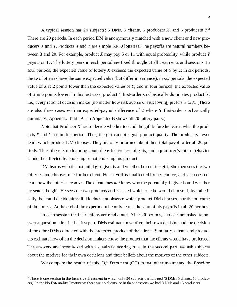
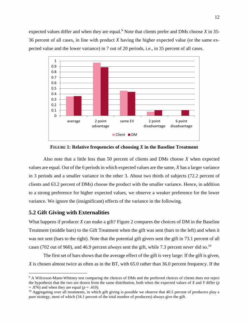
In Figure 1, we show how often product X is preferred by the client (dark red bars) and how

often it is chosen by DM (light red bars), both on average over all 20 periods and separately for

cases when the expected value of X is higher than, equal to, or lower than that of Y. These choices

serve as the benchmark for all other treatments, where producer X has the option of giving a gift.

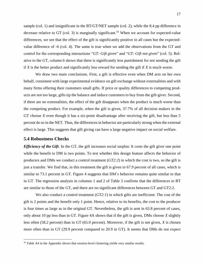
The figure shows that clients strongly prefer the lottery with the higher expected value: 97

percent prefer product X if it has the higher expected value. If the expected value of lottery X is,

instead, 2 points smaller than that of Y, only 8 percent of clients prefer X. And if X has a disad-

vantage of 6 points (and is first-order stochastically dominated by Y), no client prefers X.

The choices of decision makers are closely aligned with the preferences of clients. The

overwhelming majority chooses the lottery with the highest expected value. There is no statistically

significant difference between their choices and the preferred choices of the clients, both when

8 A related approach is “guilt aversion” (Charness and Dufwenberg, 2006): People feel guilt if they do not meet others’

expectations. This approach is not applicable since neither producer nor client learn which product DM chooses.

12

expected values differ and when they are equal.9 Note that clients prefer and DMs choose X in 35-

36 percent of all cases, in line with product X having the higher expected value (or the same ex-

pected value and the lower variance) in 7 out of 20 periods, i.e., in 35 percent of all cases.

FIGURE 1: Relative frequencies of choosing X in the Baseline Treatment

Also note that a little less than 50 percent of clients and DMs choose X when expected

values are equal. Out of the 6 periods in which expected values are the same, X has a larger variance

in 3 periods and a smaller variance in the other 3. About two thirds of subjects (72.2 percent of

clients and 63.2 percent of DMs) choose the product with the smaller variance. Hence, in addition

to a strong preference for higher expected values, we observe a weaker preference for the lower

variance. We ignore the (insignificant) effects of the variance in the following.

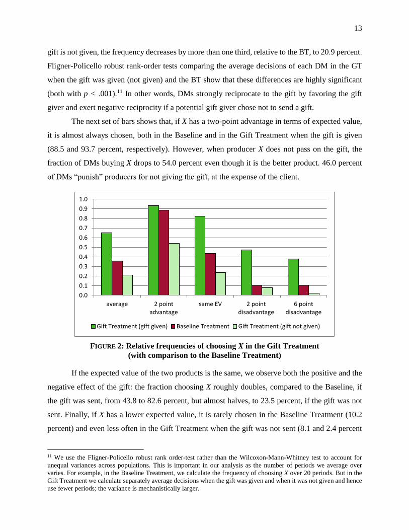
5.2 Gift Giving with Externalities

What happens if producer X can make a gift? Figure 2 compares the choices of DM in the Baseline

Treatment (middle bars) to the Gift Treatment when the gift was sent (bars to the left) and when it

was not sent (bars to the right). Note that the potential gift givers sent the gift in 73.1 percent of all

cases (702 out of 960), and 46.9 percent always sent the gift, while 7.3 percent never did so.10

The first set of bars shows that the average effect of the gift is very large: If the gift is given,

X is chosen almost twice as often as in the BT, with 65.0 rather than 36.0 percent frequency. If the

9 A Wilcoxon-Mann-Whitney test comparing the choices of DMs and the preferred choices of clients does not reject

the hypothesis that the two are drawn from the same distribution, both when the expected values of X and Y differ (p

= .876) and when they are equal (p = .410). 10 Aggregating over all treatments, in which gift giving is possible we observe that 40.5 percent of producers play a

pure strategy, most of which (34.1 percent of the total number of producers) always give the gift.

0

0.1

0.2

0.3

0.4

0.5

0.6

0.7

0.8

0.9

1

average 2 pointadvantage

same EV 2 pointdisadvantage

6 pointdisadvantage

Client DM

13

gift is not given, the frequency decreases by more than one third, relative to the BT, to 20.9 percent.

Fligner-Policello robust rank-order tests comparing the average decisions of each DM in the GT

when the gift was given (not given) and the BT show that these differences are highly significant

(both with p < .001).11 In other words, DMs strongly reciprocate to the gift by favoring the gift

giver and exert negative reciprocity if a potential gift giver chose not to send a gift.

The next set of bars shows that, if X has a two-point advantage in terms of expected value,

it is almost always chosen, both in the Baseline and in the Gift Treatment when the gift is given

(88.5 and 93.7 percent, respectively). However, when producer X does not pass on the gift, the

fraction of DMs buying X drops to 54.0 percent even though it is the better product. 46.0 percent

of DMs “punish” producers for not giving the gift, at the expense of the client.

FIGURE 2: Relative frequencies of choosing X in the Gift Treatment

(with comparison to the Baseline Treatment)

If the expected value of the two products is the same, we observe both the positive and the

negative effect of the gift: the fraction choosing X roughly doubles, compared to the Baseline, if

the gift was sent, from 43.8 to 82.6 percent, but almost halves, to 23.5 percent, if the gift was not

sent. Finally, if X has a lower expected value, it is rarely chosen in the Baseline Treatment (10.2

percent) and even less often in the Gift Treatment when the gift was not sent (8.1 and 2.4 percent

11 We use the Fligner-Policello robust rank order-test rather than the Wilcoxon-Mann-Whitney test to account for

unequal variances across populations. This is important in our analysis as the number of periods we average over

varies. For example, in the Baseline Treatment, we calculate the frequency of choosing X over 20 periods. But in the

Gift Treatment we calculate separately average decisions when the gift was given and when it was not given and hence

use fewer periods; the variance is mechanistically larger.

0.0

0.1

0.2

0.3

0.4

0.5

0.6

0.7

0.8

0.9

1.0

average 2 pointadvantage

same EV 2 pointdisadvantage

6 pointdisadvantage

Gift Treatment (gift given) Baseline Treatment Gift Treatment (gift not given)

14

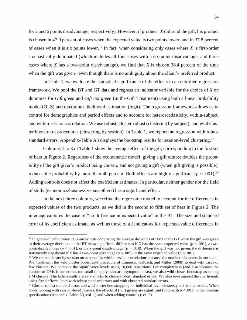
for 2 and 6 points disadvantage, respectively). However, if producer X did send the gift, his product

is chosen in 47.0 percent of cases when the expected value is two points lower, and in 37.8 percent

of cases when it is six points lower.12 In fact, when considering only cases where X is first-order

stochastically dominated (which includes all four cases with a six-point disadvantage, and three

cases where X has a two-point disadvantage), we find that X is chosen 38.4 percent of the time

when the gift was given– even though there is no ambiguity about the client’s preferred product.

In Table 1, we evaluate the statistical significance of the effects in a controlled regression

framework. We pool the BT and GT data and regress an indicator variable for the choice of X on

dummies for Gift given and Gift not given (in the Gift Treatment) using both a linear probability

model (OLS) and maximum-likelihood estimation (logit). The regression framework allows us to

control for demographics and period effects and to account for heteroscedasticity, within-subject,

and within-session correlation. We use robust, cluster-robust (clustering by subject), and wild clus-

ter bootstrap-t procedures (clustering by session). In Table 1, we report the regression with robust

standard errors. Appendix-Table A3 displays the bootstrap results for session-level clustering.13

Columns 1 to 3 of Table 1 show the average effect of the gift, corresponding to the first set

of bars in Figure 2. Regardless of the econometric model, giving a gift almost doubles the proba-

bility of the gift giver’s product being chosen, and not giving a gift (when gift giving is possible),

reduces the probability by more than 40 percent. Both effects are highly significant (p < .001).14

Adding controls does not affect the coefficient estimates. In particular, neither gender nor the field

of study (economics/business versus others) has a significant effect.

In the next three columns, we refine the regression model to account for the differences in

expected values of the two products, as we did in the second to fifth set of bars in Figure 2. The

intercept captures the case of “no difference in expected value” in the BT. The size and standard

error of its coefficient estimate, as well as those of all indicators for expected-value differences in

12 Fligner-Policello robust rank-order tests comparing the average decisions of DMs in the GT when the gift was given

to their average decisions in the BT show significant differences if X has the same expected value (p < .001), a two-

point disadvantage (p < .001), or a six-point disadvantage (p = .018). When the gift was not given, the difference is

statistically significant if X has a two-point advantage (p < .005) or the same expected value (p < .001). 13 We cannot cluster by session on account for within-session correlations because the number of clusters is too small.

We implement the wild cluster bootstrap-t procedure of Cameron, Gelbach, and Miller (2008) to deal with cases of

few clusters. We compute the significance levels using 10,000 repetitions. For completeness (and also because the

number of DMs is sometimes too small to apply standard asymptotic tests), we also wild cluster bootstrap assuming

DM clusters. The latter results are very similar to cluster-robust standard errors. We also re-estimated the coefficients

using fixed effects, both with robust standard errors and with clustered standard errors. 14 Cluster-robust standard errors and wild cluster bootstrapping for individual-level clusters yield similar results. When

bootstrapping with session-level clusters, the effects of (not) giving are significant (both with p < .001) in the baseline

specification (Appendix-Table A3, col. 1) and when adding controls (col. 2).

15

the BT (“Product X has higher/lower EV”) go in the expected direction: better products are almost

always chosen (with a probability of more than 90 percent), and worse products almost never (with

a probability of less than 10 percent). All effects are highly significant. Hence, in a world without

gifts, the influence of product value is economically and statistically highly significant.

The interaction terms in the rows below confirm the strong influence of gifts illustrated in

Figure 2. All positive and negative effects discussed above are statistically significant, regardless

of the econometric model. The insignificant or less significant coefficient estimates for (EV

[+2])*(Gift given) and (EV [-2])*(Gift not given), and (EV [-6])*(Gift not given) are cases of left-

or right-censoring: Product X is chosen almost always or almost never already in the Baseline

Treatment. Thus, passing or not passing the gift cannot significantly alter the probabilities.

Given the powerful effect of first-order stochastic dominance (FOSD) in the baseline treat-

ment, we also re-estimate our model including control variables for first order stochastic domi-

nance. We find that the FOSD effect is large and significant when we do not control for differences

in expected payoff. For example, we estimate a coefficient of 0.257 (s.e. 0.0187) and of 0.346 (s.e.

0.0230) in the model specifications of columns (1) and (2) of Table 1. However, the coefficient

becomes insignificant and shrinks by 80-90% when we control for differences in expected payoffs

of X and Y, as done in the specifications in columns (4) to (9) of Table 1. This finding suggests that

there is no significant effect of the moral wiggle room embedded in non-stochastically dominated

choices above and beyond the expected-payoff differences.

Overall, the Gift Treatment shows that gifts can have strong externalities. Clients receive

the worse product with 43 percent probability (instead of 10 percent) if the producer of the worse

product has sent a gift or the producer of the better product chose not to send a gift.

5.3 Gift Giving without Externalities

We now ask how the effects of gifts compare to a setting without externalities. If gifts have the

same effect, regardless of who pays the cost, there is no obvious distortion and it is more difficult

to argue that gifts induce inefficient behavior. If, instead, DMs act differently on their own account,

the possibility of gift giving is distortive and likely to be welfare reducing for third parties.

In the No Externality Treatment (NET) there is no client. DM decides on her own behalf

and, instead of receiving a fixed wage, is full residual claimant. Figure 3 compares the BT (middle

bars) to the NET when the gift was sent (left bars) and when it was not sent (right bars). Note that

49.1 percent of the potential gift givers (157 out of 320 cases) decide to send the gift.

16

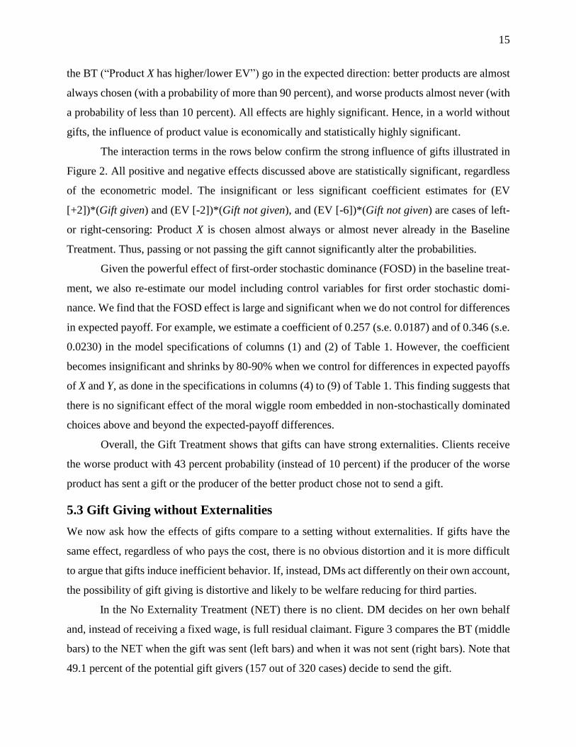
Figure 3 shows that, even when acting on their own behalf, DMs choose the potential gift

giver more often when he gives the gift (54.8 percent) than when he does not (28.8 percent) or

when there is no possibility of giving a gift (36.0 percent in the BT). However, the effects are

weaker than in the GT, where we observed an increase to 64.9 percent upon receiving the gift and

a reduction to 20.9 percent upon not receiving a possible gift. The columns to the right confirm that

DMs punish less often for not giving than in the GT in Figure 2. Also, when product X is much

worse (6 point disadvantage in expected value) the influence of the gift vanishes.15

FIGURE 3: Relative frequencies of choosing X in the No Externality Treatment

(with comparison to the Baseline Treatment)

These visual impressions are confirmed by the estimations reported in Table 2. For brevity,

we only show the linear probability model; the logit results are very similar in terms of economic

and statistical significance. All specifications include the controls for gender, economics major,

and period. The average effects are reported in columns 1 to 3. We use the pooled data of BT and

NET in column 1, and we add the GT data in columns 2 and 3. We observe a significant but smaller

increase in the frequency of choosing X when the gift is sent. Both the increase itself (amounting

to 18.4–18.7 pp) and the difference in increase relative to the GT (-10.3 pp) are highly significant.

The decrease after not receiving the gift (-6.8 to -7.1 pp) is marginally significant in the BT/NET

15 Fligner-Policello robust rank-order tests comparing the reveal that we cannot reject the hypothesis that the DMs’

decisions in GT and NET when the gift was sent are drawn from the same distribution (p = .198). When the gift was

not sent, they are significantly different (p = .032). Subsampling by EV-differences, decisions are different when the

gift was given and X has a six point disadvantage (p = .023) and when the gift was not given and X has a two-point

advantage (p = .079).

0.0

0.1

0.2

0.3

0.4

0.5

0.6

0.7

0.8

0.9

1.0

average 2 pointadvantage

same EV 2 pointdisadvantage

6 pointdisadvantage

No Externality (gift given) Baseline Treatment No Externality (gift not given)

17

sample (col. 1) and insignificant in the BT/GT/NET sample (col. 2), while the 8.4 pp difference in

decrease relative to GT (col. 3) is marginally significant.16 When we account for expected-value

differences, we see that the effect of the gift is significantly positive in all cases but the expected-

value difference of -6 (col. 4). The same is true when we add the observations from the GT and

control for the corresponding interactions “GT: Gift given” and “GT: Gift not given” (col. 5). Rel-

ative to the GT, column 6 shows that there is significantly less punishment for not sending the gift

if X is the better product and significantly less reward for sending the gift if X is much worse.

We draw two main conclusions. First, a gift is effective even when DM acts on her own

behalf, consistent with large experimental evidence on gift exchange without externalities and with

many firms offering their customers small gifts. If price or quality differences to competing prod-

ucts are not too large, gifts tip the balance and induce customers to buy from the gift-giver. Second,

if there are no externalities, the effect of the gift disappears when the product is much worse than

the competing product. For example, when the gift is given, 37.7% of all decision makers in the

GT choose X even though it has a six-point disadvantage after receiving the gift, but less than 5

percent do so in the NET. Thus, the differences in behavior are particularly strong when the external

effect is large. This suggests that gift giving can have a large negative impact on social welfare.

5.4 Robustness Checks

Efficiency of the Gift. In the GT, the gift increases social surplus: It costs the gift giver one point

while the benefit to DM is two points. To test whether this design feature affects the behavior of

producers and DMs we conduct a control treatment (GT2:2) in which the cost is two, so the gift is

just a transfer. We find that, in this treatment the gift is given in 67.9 percent of all cases, which is

similar to 73.1 percent in GT. Figure 4 suggests that DM’s behavior remains quite similar to that

in GT. The regression analysis in columns 1 and 2 of Table 3 confirms that the differences to BT

are similar to those of the GT, and there are no significant differences between GT and GT2:2.

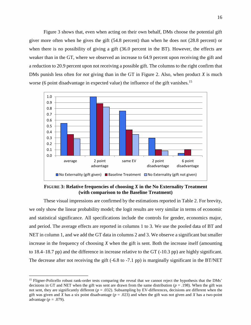
We also conduct a control treatment (GT2:1) in which gifts are inefficient: The cost of the

gift is 2 points and the benefit only 1 point. Hence, relative to its benefits, the cost to the producer

is four times as large as in the original GT. Nevertheless, the gift is sent in 63.8 percent of cases,

only about 10 pp less than in GT. Figure 4A shows that if the gift is given, DMs choose X slightly

less often (58.2 percent) than in GT (65.0 percent). Moreover, if the gift is not given, X is chosen

more often than in GT (29.9 percent compared to 20.9 in GT). It seems that DMs do not expect

16 Table A4 in the Appendix shows that session-level clustering yields very similar results.

18

producers to give the gift and do not punish them as much if gift giving is costly and inefficient.

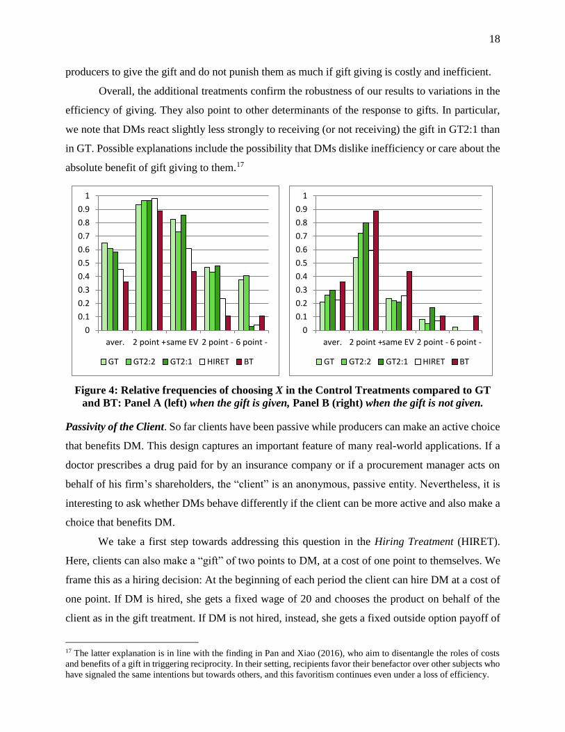
Overall, the additional treatments confirm the robustness of our results to variations in the

efficiency of giving. They also point to other determinants of the response to gifts. In particular,

we note that DMs react slightly less strongly to receiving (or not receiving) the gift in GT2:1 than

in GT. Possible explanations include the possibility that DMs dislike inefficiency or care about the

absolute benefit of gift giving to them.17

Figure 4: Relative frequencies of choosing X in the Control Treatments compared to GT

and BT: Panel A (left) when the gift is given, Panel B (right) when the gift is not given.

Passivity of the Client. So far clients have been passive while producers can make an active choice

that benefits DM. This design captures an important feature of many real-world applications. If a

doctor prescribes a drug paid for by an insurance company or if a procurement manager acts on

behalf of his firm’s shareholders, the “client” is an anonymous, passive entity. Nevertheless, it is

interesting to ask whether DMs behave differently if the client can be more active and also make a

choice that benefits DM.

We take a first step towards addressing this question in the Hiring Treatment (HIRET).

Here, clients can also make a “gift” of two points to DM, at a cost of one point to themselves. We

frame this as a hiring decision: At the beginning of each period the client can hire DM at a cost of

one point. If DM is hired, she gets a fixed wage of 20 and chooses the product on behalf of the

client as in the gift treatment. If DM is not hired, instead, she gets a fixed outside option payoff of

17 The latter explanation is in line with the finding in Pan and Xiao (2016), who aim to disentangle the roles of costs

and benefits of a gift in triggering reciprocity. In their setting, recipients favor their benefactor over other subjects who

have signaled the same intentions but towards others, and this favoritism continues even under a loss of efficiency.

0

0.1

0.2

0.3

0.4

0.5

0.6

0.7

0.8

0.9

1

aver. 2 point +same EV 2 point - 6 point -

GT GT2:2 GT2:1 HIRET BT

0

0.1

0.2

0.3

0.4

0.5

0.6

0.7

0.8

0.9

1

aver. 2 point +same EV 2 point - 6 point -

GT GT2:2 GT2:1 HIRET BT

19

18, and the product is chosen at random. The client incurs a loss due to the fact that the product is

now chosen randomly plus an additional transaction cost of three points. These design features

ensure that the total loss of not hiring DM is comparable to the cost of a producer who does not

give the gift (and is therefore chosen by DM with a lower probability).

We find that DM is hired in 92.2 percent of all cases. The fourth bars of Figure 4 (Panels A

and B) display DM’s behavior in HIRET. DMs choose the gift giver’s product in 45.1 percent of

all cases (compared to 65.0 percent in GT). Whenever the expected value of X is equal or lower

than that of Y, it is chosen much less often than in the GT after gift giving. Clearly, if the client is

in a symmetric position to the producer, the producer’s gift is less effective. This is confirmed by

the regression reported in Column 6 of Table 3. However, if the gift was not given, DMs’ behavior

in HIRET is not significantly different from that in GT, neither on average nor when considering

different expected values. Furthermore, Table 3, column 5, shows that DMs’ behavior in HIRET

is still highly significantly different from their behavior in the baseline treatment without gifts. If

clients are active, they can reduce but not fully eliminate the effects of gifts given by producers.

Large Externalities. In the Gift Treatment the externality imposed on the client by DM’s reciprocal

behavior does not exceed 6 points in expected value, which is about 40 percent of the client’s

expected payoff. To explore whether the propensity to reward gift giving persists even when the

externalities imposed on the client are very large, we conducted the Large Externality Treatment

(LET). Here, we added ten more periods to two sessions of the Gift Treatment. In six of these ten

periods the expected value of product X is 16 points lower than that of product Y. For those periods

11 percent of DMs choose X if the gift was given compared to 38 percent if the disadvantage of X

was 6 points and 47 percent if the disadvantage was 2 points.18 Eleven percent is still a significant

fraction, but the responsiveness to the gift is reduced if the externality becomes large.

5.5 Awareness

Are decision makers aware how strongly their behavior has been influenced by the gift? To answer

this question we asked them at the end of the experiment to “estimate in how many periods the

product that you chose coincided with the product your client would have chosen by himself.” We

also asked them to estimate in how many periods other decision makers had chosen the product the

client preferred. Finally, we asked clients and producers the same questions (about the decision

makers). All subjects were paid for the precision of their estimates using a quadratic scoring rule.

18 See also the regression reported in columns 7 and 8 of Table 1.

20

The result is remarkable: In the Gift Treatment DMs on average estimate that they chose

the client’s preferred product in 69.8 percent of cases; clients predict that DMs chose the preferred

product in 68.8 percent, and producers in 68.2 percent of cases. All three estimates are very close

to the actual frequency, 65.2 percent. Thus, neither DMs nor clients or producers seem to system-

atically over- or underestimate the quality of the decisions.19 However, when decision makers are

asked to estimate how often other decision makers chose the preferred product of the client, their

estimate drops to 63.1 percent. While DMs’ actual behavior is not significantly different, the dif-

ference to DMs’ estimates of their own behavior is significant at the 1 percent level.20

These results, as well as the finding that DMs match clients’ preferences almost perfectly

in the Baseline Treatment imply that DMs are well aware of being influenced by the gift. To better

understand this influence, we asked subjects at the end of the experiment several questions about

their own motivation and the perceived motivation of the other players. Subjects had to answer

these questions by choosing a natural number between 1 (= fully agree) and 6 (= do not agree at

all). If the average of the reported numbers is below 3.5, subjects tend to agree with a statement; if

the average is above 3.5, they tend to disagree. If a subject reports 1 or 2 (5 or 6), we say that this

subject “strongly agrees” (“strongly disagrees”) with the statement.

The first set of questions in the Gift Treatment refers to the motivation of the gift giver.

When asked why the producers passed on the gift, almost all decision makers strongly agree with

the statement that “the producer wants to influence my behavior” (1.63 on average). DMs are in-

different about the statement that “the producer wants to be nice to me” (3.54) and skeptical about

the statement that the producer does so for efficiency reasons because the gift is doubled and “my

gain is larger than his” (4.03). Furthermore, they do not agree with the statement that if the pro-

ducer did not pass on the gift he did so because he “does not want to leave the impression that he

wants to influence my decision” (4.75). Clients’ answers to these questions were very similar.

The perceptions of DMs and clients closely match the self-reported motivations of produc-

ers. Producers openly admit that they offered the gifts “to influence the decision of the decision

maker in my favor” (1.55), and not “to be nice” (3.91) or for efficiency reasons (4.02). They also

tend to agree with the statement that “had I not passed on the gift to the decision maker (s)he would

19 Wilcoxon-Mann-Whitney tests comparing the decisions of DMs with the predictions of the clients or of the producers

do not reject the hypothesis that they are drawn from the same distribution (p = .510 and p = .393, respectively). 20 A Wilcoxon signed rank test comparing the decisions of DMs and the predictions of DMs about the behavior of

other DMs do not reject the hypothesis that the two are drawn from the same distribution (p = .520). A Wilcoxon

signed rank test comparing the predictions of DMs about their own behavior and about the behavior of other DMs

rejects the hypothesis that the two are drawn from the same distribution at p = .001.

21

not have bought my product” (2.47). In summary, producers pass on the gift because they want to

influence the DM’s behavior and because they are afraid that otherwise DMs will not buy their

product; DMs and clients perceive this motivation correctly. Nevertheless, DMs respond to the gift.

We also asked DMs directly whether their “decisions have never been influenced by the

premium.” About a third of subjects (31.3 percent) deny any influence. More than half (54.2 per-

cent) openly admit that their decisions have been strongly affected. More than half also agree

strongly with a similar statement about not receiving the gift, “When one of the producers did not

pass on the gift even though he could have done so, I did not buy his product.” Furthermore, when

asked whether they believe that other DMs have been influenced, they agree even more strongly.

What motivation explains the influence of the gift? In a last set of questions, we elicited

DMs’ emotions towards the gift giver. We find that, among those (54.2 percent) who admit to being

influenced, 88 percent report positive emotions towards the gift giver or a sense of obligation to

buy his product.21 At the same time, all of these 88 percent tend to agree with the statement that

the gift was given because “the producer wants to influence my behavior”, 91 % even strongly so.

6 A Model of Social Preferences with Endogenous Reference Groups

The experimental results show a clear pattern of reciprocal behavior. DMs favor producer X if he

gives the gift, and they discriminate against him if he does not. This contradicts standard theories

of outcome-based social preferences such as altruism, maximin preferences, and inequality aver-

sion, as well as type-based models of reciprocity that all predict that DM favors the client. Inten-

tion-based reciprocity is consistent with the observed behavior, but also with the opposite. Further-

more, the experiments show that decision makers are fully aware that producers give the gift not

because they are kind, but because they want to influence their behavior at the expense of their

clients. Thus, gift giving is interpreted by the decision makers as a selfish act of the producer.

Why, then, is gift giving so effective? DMs report feeling more positive towards the gift

giver and a sense of obligation to reciprocate even though they understand the intentions of the

giver. The anthropological and sociological literature is well aware of the fact that gifts create an

obligation that is independent of the intention of the gift giver. In a highly influential essay, the

anthropologist Mauss (1924) argues that in archaic societies humans are under an obligation to

21 When asked whether they “liked a producer who passed on the gift better than the other producer,” 88 percent of

DMs tend to agree. When asked whether they “felt obliged to buy the product” of the gift giver, again 65 percent tend

to agree, and when asked whether the gift giver “deserves that his product is bought,” 54 percent tend to agree.

22

give, to receive, and then to repay.22 Prominent sociologists such as Gouldner (1960) and Blau

(1964) argue that reciprocity is a universal social norm that is not just enforced by social pressure

and self-interest to maintain a mutually beneficial relationship, but is internalized.23 This view of

a gift as creating a bond and an obligation to reciprocate captures the observed behavior better than

theories of reciprocity that are based on income distribution, type, or intentions.

In the following we propose a simple extension of outcome-based models of social prefer-

ences that formalizes this view. Suppose that, initially, DM is equally concerned about the payoffs

of all other players. If another player increases DM’s payoff (and if DM did not perfectly anticipate

this), that player gets a higher weight in DM’s utility function. If a player reduces DM’s payoff (as

compared to DM’s expectation), the player gets a lower (possibly negative) weight. The key inno-

vation, relative to existing models of “action-based reciprocity” is that the weight producer X gets

in DM’s utility depends not only on what producer X does, but also on what DM expects him to

do.24 If an action was expected with a high probability, the action has less of an effect than if it was

expected with a small probability. We endogenize the “reference group” that each player cares

about by making the weight on the material payoff of a player in the utility function of another

player dependent on the actions of the former and the expectations of the latter.

Formally, consider an N-player game of perfect information. Player i{1,…, N} chooses

strategy si out of his strategy set Si. Let s = (s1,…,sN) denote a pure strategy profile of all players.

As in Section 4, we assume that all parties are risk neutral. The utility of player i is given by

( ) ( ) ( ),i i j j

i

j i

U m s s m s

(2)

where 𝛼𝑖𝑗(𝑠|𝜎) is the weight player i puts on the payoff of player j. Thus, i’s utility depends not

only on his own material payoff mi(s), which is a function of the strategies chosen by all players,

but also on the material payoffs of all other players. What is new here is that the weights of these

22 Mauss (1924) was inspired by Malinowski’s (1922) anthropological field study of the Trobrianders (islanders in the

Western Pacific) that identifies 80 forms of social and economic exchange as based on reciprocity. 23 See also experiments in the social psychology literature (e.g., Whatley et al. 1999). Kolm (2006) argues that people

have positive emotions towards a gift giver and feel “moral indebtedness.” Synonyms for saying “thank you” reflect

this insight: “much obliged” in English, “je vous suis très obligé” in French, and “ich bin Ihnen sehr verbunden”

(literally: “I am bound to you”) in German. The effectiveness of gifts and compliments even if the recipient is aware

of ulterior motives, is a building block of “ingratiation” in social psychology (Jones 1964). People comply with re-

quests from those who have done them a favor, even if the favor was unsolicited and if they do not like the gift giver

(Regan 1971, Cialdini 1993). 24 The action-based model Cox et al (2008) is different also in that it is restricted to two-stage games with two players

and perfect information. Cf. also Cox et al (2007) and the concept of “social ties” in Van Dijk and van Winden (1997).

23

payoffs in i ’s utility function depend on how the strategies chosen compare to the “expected” strat-

egies. The “expected” strategy profile σ is a (possibly mixed) strategy profile expected to be played

in the game, e.g., because of past experience in similar circumstances, or because σ constitutes a

social norm, or because σ is an equilibrium of the game that players expect to be played.

Assumption 1: A player has social preferences over an endogenously formed reference group that

can be represented by (2). If player j chooses a pure strategy sj that increases (decreases) player i’s

payoff compared to the (expected) payoff that i would have received if j had chosen the expected

strategy σj, then the weight of player j’s payoff in player i’s utility increases (decreases) compared

to the weight if j had chosen σj: ( , ) ( ) ( , )i i

j j j jm s m ( , ) ( ) ( )j j

i j j is .

Let us apply this simple model to our gift giving game. Suppose that in the Baseline Treat-

ment where no gift can be made DM puts equal weight α on the client and on producers X and Y,

i.e., 0 Y

DM

X

DM

C

DM . This implies that DM favors the client. Consider now the Gift

Treatment and the No Externality Treatment, and suppose DM expects that the gift is given with

probability X (0,1). Thus, if producer X gives the gift, DM’s payoff increases to 20 + 2 as com-

pared to what she expected, 20+2X; so the weight that she attaches to the welfare of producer X

also increases, )|( X

X

DM gg , where gg indicates “gift given.” If producer X does not give the

gift, DM’s payoff decreases (to 20), compared to what she expected, so the weight that she attaches

to producer X also decreases, )|( X

X

DM gng , where gng indicates “gift not given.”

In the following, we assume for simplicity that )|( X

X

DM gg = k , with 0 < α < 1, and

where 1k is distributed across subjects according to some cdf F k , and )|( X

X

DM gng =

l, where 0 ≤ l ≤ 1 is distributed according to some cdf G(l).

Proposition 4. Consider a decision maker with social preferences satisfying Assumption 1.

(i) Suppose producer X passes on the gift. If product X is (weakly) better than product Y, DM

always chooses X in GT and NET. If product X is strictly worse, DM may still choose X, and

she is more likely to do so if the payoff goes to a third person (GT) than if it goes to herself

(NET).

(ii) Suppose that producer X does not pass on the gift. If X is (weakly) worse than Y, DM always

chooses Y in GT and in NET. If X is strictly better, DM may still choose Y, and she is more

likely to do so if the payoff goes to a third person (GT) than if it goes to herself (NET).

24

Proof: See Appendix A.

The intuition for these results is straightforward. If producer X sends the gift, his weight in

DM’s utility function increases from α to kα. Thus, if X is the better product, DM chooses X in GT

and in NET as this choice allows him both to reciprocate towards the gift giver and to benefit her

client. If producer X passes on the gift but X is the worse product, DM chooses X in GT if k is large

enough to offset the utility loss of the client. In NET DM buys the product for herself, so she has a

stronger financial incentive to choose the better product. However, if product X is not much worse

than Y, and if k is sufficiently large, DM may still favor producer X since the gift giver gains 16

while the financial cost of reciprocity is small. The argument for case (ii) is analogous.

To transform the above framework into a testable theory we need an ex-ante measure for

the “expected behavior.” Only given such a measure, we can test whether the weight that the DM

puts on the gift giver in her utility function depends on whether and, in the more general version

of the model, by how much he exceeded or disappointed her expectations.

One simple proxy for such expectations could be the actual empirical frequency of giving.

Remember, for example, that increasing efficiency induces an increase in giving from 63.8 percent

in GT2:1 to 67.9 percent in GT2:2 and 73.1 percent in GT. We can make use of this variation to

test whether the gift effect depends on how much gift-giving exceeds, or falls short of, expectations

by including the relative frequency of gift giving in a given treatment as one of the independent

variables. (Note that, for such an analysis, we return to a more general version of the model, where

the weight 𝛼𝑖𝑗(𝑠|𝜎) that player i puts on the payoff of player j can depend on by how much the j

has exceeded or disappointed i's expectations, rather than fixing those weights at k and l.)

In Table 4, we estimate the same linear regression model as before but with the added proxy

and including data only from treatments where gift giving is possible, namely, GT2:1, GT2:2 and

GT as well as LGT (which we will discuss in Section 7.2). We find that the estimated coefficient

for the relative frequency of gift giving is significantly different from zero and sizeable for all

specifications. As the model predicts, it is negative, i.e., in a setup were gifts are less likely, reac-

tions to them are stronger. In terms of magnitude, the coefficient is very stable, around 0.28,

regardless of whether we include no additional controls (column 1) or a full slate of additional

controls (column 3). In other words, if we raise the expectation of receiving a gift, as proxied by

the average frequency of producers sending a gift across a treatment, from 0 to 1, we reduce the

response to the gift by about 28 pp. An increase of one standard deviation (which is 9% across

25

these treatments) reduces the response to the gift by 2 pp).25

As an alternative proxy for expectations, one may postulate that expectations are most af-

fected by a subject’s personal experience of receiving gifts so far. A DM who has received gifts

with a high frequency in the past, might have high expectations and thus respond less positively to

the next gift and more negatively to not receiving a gift. To test for such dynamic effects in recip-

rocation and punishment, we re-estimate our baseline model on the sample of treatments with gift

giving but include the relative frequency of having received gifts prior to the current round as an

explanatory variable.26 (As this cannot be defined in a meaningful way for the first period, we do

exclude period 1 in these regressions.) Using this alternative proxy, we have more variation across

observations, with a mean experience of 0.753 and a standard deviation of 0.213 for the sample in

Table 4. The within-subject variation also allows us to include treatment fixed effects. As the last

two columns of Table 4 reveal, we estimate again the expected negative relationship. There is a

significant negative effect of past gifts on the positive response to a current gift. The coefficient

estimates indicate that increase in past gifts by one standard deviation reduces the response to the

gift by 3 to 4 pp.

Hence, our conceptual framework appears to offer promise to provide the foundation for a

testable model of the formation of reference groups for and strength of social preferences.

7 Policy Treatments

Most of the remedies proposed in practice to deal with the problem of gift giving fall in two broad

categories: disclosure and size limits. The idea of disclosure is to raise awareness about the poten-

tial influence of the gift. For example, in the US and many European countries political parties and

individual politicians have to disclose campaign contributions so that voters can see which interest

groups supported them. Another prominent example is the Physician Payment Sunshine Act in the

US by which the government requires physicians to report annually all payments over a cumulative

value of $100 and which, since September 30, 2014, is made available to the public.27 The idea of

size limits is to reduce the influence of gift givers. For example, in California, local elected officials

25 Of course, this coefficient captures other treatment differences, too. However, in additional (unreported) regressions

that include data from all treatments except BT, the coefficients remain significant and sizably negative, even though

the comparison weight of the client changes as he assumes an active role (in HIRET and IT). 26 We thank one of our anonymous referees for this suggestion. 27 See p. 9503 of the final rule at www.cms.gov/Regulations-and-Guidance/Legislation/National-Physician-Payment-

Transparency-Program/Downloads/Affordable-Care-Act-Section-6002-Final-Rule.pdf, last accessed 11/6/2016.

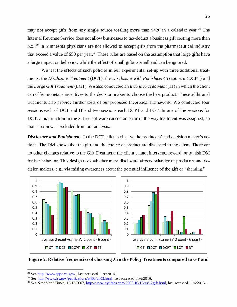
26

may not accept gifts from any single source totaling more than $420 in a calendar year.28 The

Internal Revenue Service does not allow businesses to tax-deduct a business gift costing more than

$25.29 In Minnesota physicians are not allowed to accept gifts from the pharmaceutical industry

that exceed a value of $50 per year.30 These rules are based on the assumption that large gifts have

a large impact on behavior, while the effect of small gifts is small and can be ignored.

We test the effects of such policies in our experimental set-up with three additional treat-

ments: the Disclosure Treatment (DCT), the Disclosure with Punishment Treatment (DCPT) and

the Large Gift Treatment (LGT). We also conducted an Incentive Treatment (IT) in which the client

can offer monetary incentives to the decision maker to choose the best product. These additional

treatments also provide further tests of our proposed theoretical framework. We conducted four

sessions each of DCT and IT and two sessions each DCPT and LGT. In one of the sessions for

DCT, a malfunction in the z-Tree software caused an error in the way treatment was assigned, so

that session was excluded from our analysis.

Disclosure and Punishment. In the DCT, clients observe the producers’ and decision maker’s ac-

tions. The DM knows that the gift and the choice of product are disclosed to the client. There are

no other changes relative to the Gift Treatment: the client cannot intervene, reward, or punish DM

for her behavior. This design tests whether mere disclosure affects behavior of producers and de-

cision makers, e.g., via raising awareness about the potential influence of the gift or “shaming.”

Figure 5: Relative frequencies of choosing X in the Policy Treatments compared to GT and

28 See http://www.fppc.ca.gov/ , last accessed 11/6/2016. 29 See http://www.irs.gov/publications/p463/ch03.html, last accessed 11/6/2016. 30 See New York Times, 10/12/2007, http://www.nytimes.com/2007/10/12/us/12gift.html, last accessed 11/6/2016.

0

0.1

0.2

0.3

0.4

0.5

0.6

0.7

0.8

0.9

1

average 2 point +same EV 2 point - 6 point -

GT DCT DCPT LGT BT

0

0.1

0.2

0.3

0.4

0.5

0.6

0.7

0.8

0.9

1

average 2 point +same EV 2 point - 6 point -

GT DCT DCPT LGT BT

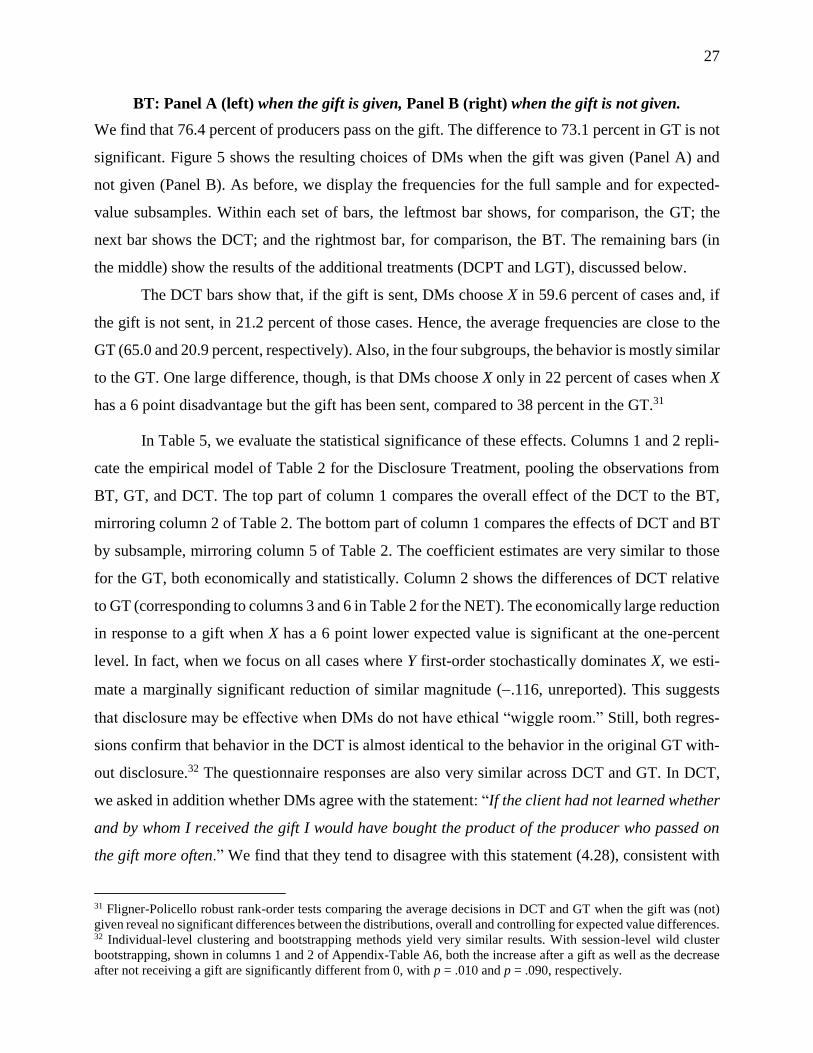
27

BT: Panel A (left) when the gift is given, Panel B (right) when the gift is not given.

We find that 76.4 percent of producers pass on the gift. The difference to 73.1 percent in GT is not

significant. Figure 5 shows the resulting choices of DMs when the gift was given (Panel A) and

not given (Panel B). As before, we display the frequencies for the full sample and for expected-

value subsamples. Within each set of bars, the leftmost bar shows, for comparison, the GT; the

next bar shows the DCT; and the rightmost bar, for comparison, the BT. The remaining bars (in

the middle) show the results of the additional treatments (DCPT and LGT), discussed below.

The DCT bars show that, if the gift is sent, DMs choose X in 59.6 percent of cases and, if

the gift is not sent, in 21.2 percent of those cases. Hence, the average frequencies are close to the

GT (65.0 and 20.9 percent, respectively). Also, in the four subgroups, the behavior is mostly similar

to the GT. One large difference, though, is that DMs choose X only in 22 percent of cases when X

has a 6 point disadvantage but the gift has been sent, compared to 38 percent in the GT.31

In Table 5, we evaluate the statistical significance of these effects. Columns 1 and 2 repli-

cate the empirical model of Table 2 for the Disclosure Treatment, pooling the observations from

BT, GT, and DCT. The top part of column 1 compares the overall effect of the DCT to the BT,

mirroring column 2 of Table 2. The bottom part of column 1 compares the effects of DCT and BT

by subsample, mirroring column 5 of Table 2. The coefficient estimates are very similar to those

for the GT, both economically and statistically. Column 2 shows the differences of DCT relative

to GT (corresponding to columns 3 and 6 in Table 2 for the NET). The economically large reduction

in response to a gift when X has a 6 point lower expected value is significant at the one-percent

level. In fact, when we focus on all cases where Y first-order stochastically dominates X, we esti-

mate a marginally significant reduction of similar magnitude (.116, unreported). This suggests

that disclosure may be effective when DMs do not have ethical “wiggle room.” Still, both regres-

sions confirm that behavior in the DCT is almost identical to the behavior in the original GT with-

out disclosure.32 The questionnaire responses are also very similar across DCT and GT. In DCT,

we asked in addition whether DMs agree with the statement: “If the client had not learned whether

and by whom I received the gift I would have bought the product of the producer who passed on

the gift more often.” We find that they tend to disagree with this statement (4.28), consistent with

31 Fligner-Policello robust rank-order tests comparing the average decisions in DCT and GT when the gift was (not)

given reveal no significant differences between the distributions, overall and controlling for expected value differences. 32 Individual-level clustering and bootstrapping methods yield very similar results. With session-level wild cluster

bootstrapping, shown in columns 1 and 2 of Appendix-Table A6, both the increase after a gift as well as the decrease

after not receiving a gift are significantly different from 0, with p = .010 and p = .090, respectively.

28

their observed behavior. These results suggest that disclosing gift givers alone may generally not

be an effective way to discipline the behavior of the recipient.

In the second disclosure treatment (DCPT), we added the possibility to punish DM for her

choice of product. The client can reduce DM’s payoff by one point, at the cost of ½ point to himself.

The information structure is as in DCT: the client is informed about the behavior of X and DM.

The possibility of being punished does not deter producers: 74.3 percent pass on the gift.

Moreover, the third bars of Figure 5 reveal that DMs’ choices remain very similar to DCT. DMs

choose X in 57.1 percent of all cases when the gift was given (compared to 59.6 and 65.0 percent

in the DCT and GT, respectively). When the gift was not given, 27.6 percent (24.7 and 21.2 percent

in DCT and GT, respectively) choose X. It seems that the introduction of a small punishment device

in addition to a disclosure does not alter DMs’ behavior much. The regression analysis for DCPT

in Table 5 (col. 3-5) confirms this impression. In particular, the regression comparing DCPT to

DCT (col. 5) reveals that there is no significant difference; none of the coefficients of the dummy

variables containing DCPT are significantly different from zero. One reason for this limited influ-

ence of punishment may be that decision makers correctly anticipate that clients will seldom make

use of it. Overall, clients in the DCPT punish in only 7.5 percent of all periods.33

As a caveat, we emphasize that disclosure to peers of a DM may have more powerful sham-

ing effects in practice – at least if there is a strong enough norm of treating clients well. Lacking

an environment that reflects the prevalent social norm in a community, as well as for anonymity

reasons, public “shaming” is not readily implementable in a laboratory setting. Still, our laboratory

results reveal the limits of disclosure in effectively altering behavior.

Size of the Gift. In the LGT. we triple the benefit of the gift keeping its cost constant.34 If producer

X spends 1 point DM receives 6 (rather than 2) points, almost one third of her fixed wage of 20.

The LGT allows us to test whether large gifts have a stronger effect on behavior than small gifts.

Because the (relative) price of gift giving is reduced it is not surprising that producers send

the gift more often. In 92.1 percent of cases, potential gift givers pass on the gift, compared to 73.1

33 We have also conducted a variant where the client has no information about the product (DCPT-PI): In two additional

sessions with 48 subjects, shown in Appendix-Table A7, the treatment resembled DCPT except for the following

aspect: The client does not know the identity of the gift giver and which product was chosen and, hence, cannot con-

dition his decision to punish on whether DM was influenced to his advantage or disadvantage. Here clients almost

never punish (in only 2.9 percent of cases). Interestingly, DMs choose the gift giver’s product more often compared to

GT and DCT, both when the gift was given (73.9 percent) and when it was not given (25.3 percent). Overall, the results

are not straightforward to interpret and neither support nor contradict our model. 34 In treatments GT2:2 and GT2:1, discussed in Section 5.4.1, we doubled and quadrupled the cost of the gift, relative

to the benefit, which had very little effect on the behavior of the producer and DM.

29

percent in the GT. Furthermore, producers strongly confirm in the questionnaire that they passed

on the gift to influence DM (average answer of 1.25 as compared to 1.55 in GT), and they strongly

negate that the gift has no impact (average answer of 5.13 as compared to 4.52 in GT). Similarly,

more clients are strongly convinced that the gift influences the decision maker in the Large Gift

Treatment (75 percent) than in the Gift Treatment (52 percent).

Perhaps surprisingly, DMs respond significantly less to the larger gift, as shown in Figure

5 and Table 5 (col. 6-7). When the gift is passed on, DMs choose X in 53.4 percent of cases, com-

pared to 65.0 percent in GT.35 The difference in coefficients is highly significant (p <.01) (col. 2,

top part).36 If product X is worse than Y, the effect of the gift is about half as strong in LGT as in

GT, and is significant at the 5 percent level, both for a six-point and a two-point disadvantage. The

difference between LGT and GT in the average effect of not passing on the gift is insignificant.

While it may be surprising at first glance that the effect of a large gift is weaker than the

effect of a small gift, this result is consistent with our theory in Section 6. Recall that the gift is

passed on in 92.1 percent of all cases in LGT but only in 73.1 percent in GT. Thus, the pure strategy

sj of giving the gift is much closer to the expected strategy σj in LGT than in GT, and the model

predicts that decision makers will react less to it. Similarly, not giving the gift in LGT is farther

from the expected strategy σj in LGT than in GT, and therefore the model predicts that decision

makers will react more negatively to not receiving the gift in LGT than in GT.37

This finding does not imply that size limits are useless. However, it suggests that size limits

on gifts may be insufficient to mitigate the effects of gift giving. In fact, our results show that small

gifts may have an even stronger reciprocal effect than large gifts.

Profit Sharing. A classical economic approach to counteract the gift effect is to align DM’s incen-

tives with the client’s payoff. In the Incentive Treatment (IT), we allow the client to give 10 percent

of profits to DM (without knowing whether the producer offers a gift or not). He bears half of the

cost, i.e., loses 5 percent of profits. This cost structure makes the reward symmetric to the gift of

35 A Fligner-Policello robust rank-order test comparing the average decisions of each DM when the gift was given in

the GT and the LGT shows that these differences are significant with p = .042. 36 Individual-level clustering and bootstrapping methods reach very similar results. For example, with session-level

wild cluster bootstrapping, the increase after a gift in col. 6 (top part) of Appendix-Table A6 and the difference in

increase relative to GT (col. 4, top part) are both marginally significant with p = .076 and p = .099, respectively. 37 It is interesting to note that in the LGT only 41.7 percent of DMs admit to being influenced by the gift (as compared

to 54.2 percent in GT), and those who do report being influenced admit to feeling bad about this (average 2.2 as

compared to 4.5 in GT). An alternative explanation for the size effect, then, is that the salience of the intention is

important. Because a large gift is a more salient indicator that the gift giver wants to influence the behavior of the

decision maker (the gift looks more like a bribe), some DMs resist this influence more strongly.

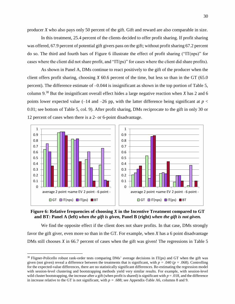
30

producer X who also pays only 50 percent of the gift. Gift and reward are also comparable in size.

In this treatment, 25.4 percent of the clients decided to offer profit sharing. If profit sharing

was offered, 67.9 percent of potential gift givers pass on the gift; without profit sharing 67.2 percent

do so. The third and fourth bars of Figure 6 illustrate the effect of profit sharing (“IT(nps)” for

cases where the client did not share profit, and “IT(ps)” for cases where the client did share profits).

As shown in Panel A, DMs continue to react positively to the gift of the producer when the

client offers profit sharing, choosing X 60.6 percent of the time, but less so than in the GT (65.0

percent). The difference estimate of –0.044 is insignificant as shown in the top portion of Table 5,

column 9.38 But the insignificant overall effect hides a large negative reaction when X has 2 and 6

points lower expected value (–14 and –26 pp, with the latter difference being significant at p <

0.01; see bottom of Table 5, col. 9). After profit sharing, DMs reciprocate to the gift in only 30 or

12 percent of cases when there is a 2- or 6-point disadvantage.

Figure 6: Relative frequencies of choosing X in the Incentive Treatment compared to GT

and BT: Panel A (left) when the gift is given, Panel B (right) when the gift is not given.

We find the opposite effect if the client does not share profits. In that case, DMs strongly

favor the gift giver, even more so than in the GT. For example, when X has a 6 point disadvantage

DMs still chooses X in 66.7 percent of cases when the gift was given! The regressions in Table 5

38 Fligner-Policello robust rank-order tests comparing DMs’ average decisions in IT(ps) and GT when the gift was

given (not given) reveal a difference between the treatments that is significant, with p = .040 (p = .068). Controlling

for the expected-value differences, there are no statistically significant differences. Re-estimating the regression model

with session-level clustering and bootstrapping methods yield very similar results. For example, with session-level

wild cluster bootstrapping, the increase after a gift (when profit is shared) is significant with p = .018, and the difference

in increase relative to the GT is not significant, with p = .688; see Appendix-Table A6, columns 8 and 9.

0

0.1

0.2

0.3

0.4

0.5

0.6

0.7

0.8

0.9

1

average 2 point +same EV 2 point - 6 point -

GT IT(nps) IT(ps) BT

0

0.1

0.2

0.3

0.4

0.5

0.6

0.7

0.8

0.9

1

average 2 point +same EV 2 point - 6 point -

GT IT(nps) IT(ps) BT

31

(lower part, col. 10-11) confirm that both the increases over the BT, estimated to be 56.4 pp, and

over the GT, estimated to be 29.0 pp, are highly significant.39 The same holds when considering all

periods in which X is first-order stochastically.

In summary, if the client offers profit sharing, DMs react positively to the gift but less so

than in the GT, and the effect of the gift vanishes when product X is much worse than product Y.

This is similar to the No Externality Treatment. However, if the client does not offer profit sharing,

the effect of the gift is even stronger than in the GT, in particular when X is much worse than Y.

Thus, the possibility of profit sharing can backfire – DMs punish clients for not sharing profits.40

These effects are consistent with our theory. As shown in Appendix A (Proposition 5), our

model predicts that the gift effect is moderated if the client shares profits, but it is exacerbated if

he does not share. Intuitively, the client strengthens the bond between him and DM by sharing, so

his weight in DM’s utility function increases. The opposite happens when profits are not shared –

the bond is weakened and the weight decreases.41 This interpretation is also consistent with the

questionnaire evidence. The large majority of subjects confirm that they have been influenced by

the additional profit sharing of the client. Almost all of them (95.7 percent) believe that the client

offered the additional reward in order to give the decision maker better incentives to choose the

best product for him, and most clients strongly confirm that this is their dominant motive.

The main conclusion from the Incentive Treatment is that rewards aligning the interests of

decision maker and client can be highly effective. However, once decision makers become aware

that clients could offer profit sharing, they punish clients for not offering the additional reward.

39 Fligner-Policello robust rank-order tests comparing DMs’ average decisions in GT and IT(nps) show that these

differences are statistically significant if the gift is not given (p = .022). Controlling for differences in expected values,

we find statistically significant differences if the gift is not given and X has either a two point advantage (p = .056) or

a six point disadvantage (p = .029). Re-estimating the regression model with session-level wild cluster bootstrapping,

the increase after a gift (when profit not shared) is significant (p = .019) while the difference in increase relative to the

GT is marginally significant (p = .089); see Appendix-Table A6, columns 10-11. 40 We also conducted two variants of the incentive treatment (with 2 sessions, 48 subjects each), shown in Appendix-

Table A7. In the first treatment (Automatic Incentive Treatment, AIT) 10 percent of the client’s profit are added auto-

matically to DM’s payoff in each period, at no cost to the client. Here, the gift is given in 61 percent of cases. The gift

still has a strong and significant effect, both in the positive and (if not given) in the negative direction, though the

positive effect is significantly smaller than in the GT. In the second treatment (Small Incentive Treatment, SIT) the

setup is the same except that DM receives the profit share for only one out of 20 periods that is determined randomly

at the end of the experiment. In this treatment the gift is given in 77 percent of cases, about as often as in the GT (73

percent). DM behavior in this treatment is similar to that in GT when the gift has been given. Surprisingly, when the

gift has not been given, DM chooses X more often. 41 Note that DMs punish clients who do not share profits rather harshly when the gift is not given (see Figure 4.B,

especially if X is the worse product). In the context of our model, the decrease in α associated with a non-sharing client

is larger in magnitude than the decrease in α associated with a producer who does not send the gift. This could be a

result of how profit sharing and gift giving are framed. Profit sharing could be perceived as a good (business) practice

that clients should undertake, while gift giving may be seen as bribery and therefore an unfavorable business practice.

32

8 Conclusions

This paper fills a critical gap in the literature on social preferences: the analysis of reciprocal be-

havior with negative external effects. A person may be “kind” because he wants to influence a

decision in his favor at the detriment of a third party. Such situations are common in many indus-

tries and other settings (such as lobbyism), but the motivating behavioral forces are underexplored.

We have shown that the possibility of gift giving causes a change in behavior. Gifts induce

decision makers to favor the gift giver. If a gift is not given, decision makers discriminate against

him, both at the expense of the third party. Gifts are also effective when the decision maker buys

the product for herself, but the effect is weaker, in particular when the gift giver’s product is much

worse. Standard models of social preferences have difficulties explaining the observed behavior. It

is better described by anthropological and sociological theories arguing that gifts create an obliga-

tion to reciprocate. A simple extension of standard models of social preferences captures this effect.

How to mitigate the effect of gifts is an important policy issue. Our results show that small

gifts can have a large impact, even if they are given unconditionally in a one-shot relationship and

if the gift cannot convey any information. In our experimental setup disclosure and size limits do

not reduce the effects of gifts while financial incentives can be highly effective. However, intro-

ducing the possibility of financial incentives is a two-sided sword. Once decision makers are aware

that additional rewards can be offered they expect them to be given and punish the client for not

doing so. It is also worth noting that the cumulative implementation of several of the non-financial

policy variations (hiring, disclosure, punishment) might yield a similar effect. A more systematic

analysis of possible remedies in the lab and in the field is an important topic for future research.

References

Abbink, Klaus. 2004. “Staff Rotation as an Anti-Corruption Policy: an Experimental Study.” Eu-

ropean Journal of Political Economy 20 (4): 887–906.

Abbink, Klaus, Bernd Irlenbusch, and Elke Renner. 2002. “An Experimental Bribery Game.”

Journal of Law, Economics, and Organization 18 (2): 428–54.

Akerlof, George A. 1982. “Labor Contracts as Partial Gift Exchange.” The Quarterly Journal of

Economics 97 (4): 543–69.

Andreoni, James, and John H. Miller. 2002. “Giving According to GARP: an Experimental Test

of the Consistency of Preferences for Altruism.” Econometrica 70 (2): 737–53.

Blau, Peter. 1964. Exchange and Power in Social Life. New York: Wiley.

Blumenthal, David. 2004. “Doctors and Drug Companies.” N Engl J Med 351 (18): 1885–90.

33

Bolton, Gary E., and Axel Ockenfels. 2000. “ERC: a Theory of Equity, Reciprocity, and Compe-

tition.” The American Economic Review 90 (1): 166–93.

Cameron, A. C., Jonah B. Gelbach, and Douglas L. Miller. 2008. “Bootstrap-Based Improve-

ments for Inference with Clustered Errors.” The Review of Economics and Statistics 90 (3):

414–27.

Campbell, Eric G., Russell L. Gruen, James Mountford, Lawrence G. Miller, Paul D. Cleary, and

David Blumenthal. 2007. “A National Survey of Physician-Industry Relationships.” New Eng-

land Journal of Medicine 356 (17): 1742–50.

Charness, Gary, and Martin Dufwenberg. 2006. “Promises and Partnership.” Econometrica 74

(6): 1579–1601.

Charness, Gary, and Matthew Rabin. 2002. “Understanding Social Preferences with Simple

Tests.” The Quarterly Journal of Economics 117 (3): 817–69.

Cialdini, Robert B. 1993. Influence: the Psychology of Persuasion. New York: Quill William

Morrow.

Cox, James C., Daniel Friedman, and Steven Gjerstad. 2007. “A Tractable Model of Reciprocity

and Fairness.” Games and Economic Behavior 59 (1): 17–45.

Cox, James C., Daniel Friedman, and Vjollca Sadiraj. 2008. “Revealed Altruism.” Econometrica

76 (1): 31–69.

Currie, Janet, Wanchuan Lin, and Juanjuan Meng. 2013. “Social networks and externalities from

gift exchange: Evidence from a field experiment.” Journal of Public Economics 107:19–30.

Dana, Jason, and George Loewenstein. 2003. “A Social Science Perspective on Gifts to Physi-

cians from Industry.” JAMA 290 (2): 252–55.

Davidson, Russell, and Emmanuel Flachaire. 2008. “The Wild Bootstrap, Tamed at Last.” Jour-

nal of Econometrics 146 (1): 162–69.

Dufwenberg, Martin, and Georg Kirchsteiger. 2004. “A Theory of Sequential Reciprocity.”

Games and Economic Behavior 47 (2): 268–98.

Fehr, Ernst, Lorenz Goette, and Christian Zehnder. 2009. “A Behavioral Account of the Labor

Market: the Role of Fairness Concerns.” Annual Review of Economics 1 (1): 355–84.

Fehr, Ernst, Georg Kirchsteiger, and Arno Riedl. 1993. “Does Fairness Prevent Market Clearing?

an Experimental Investigation.” The Quarterly Journal of Economics 108 (2): 437–59.

Fehr, Ernst, and Klaus M. Schmidt. 1999. “A Theory of Fairness, Competition, and Coopera-

tion.” The Quarterly Journal of Economics 114 (3): 817–68.

Fischbacher, Urs. 2007. “z-Tree: Zurich Toolbox for Ready-Made Economic Experiments.” Ex-

perimental Economics 10 (2): 171–78.

Gouldner, Alvin W. 1960. “The Norm of Reciprocity: a Preliminary Statement.” American Socio-

logical Review 25 (2): 161–78.

Grande, David. 2009. “Limiting the Influence of Pharmaceutical Industry Gifts on Physi-

cians: Self Regulation of Government Intervention?” Journal of General Internal Medicine 25

(1): 79–83.

34

Greiner, Ben. 2004. “An Online Recruitment System for Economic Experiments.” In Forschung

und wissenschaftliches Rechnen, edited by Kurt Kremer and Volker Macho, 79–93. GWDG

Bericht 63. Göttingen.

Jones, Edward E. 1964. Ingratiation: A Social Psychology Analysis. New York: Appleton-Cen-

tury-Croft.

Katz, Dana, Arthur L. Caplan, and Jon F. Merz. 2003. “All Gifts Large and Small.” The Ameri-

can Journal of Bioethics 3 (3): 39–46.

Kolm, Serge-Christophe. 2006. “Reciprocity: Its Scope, Rationales, and Consequences.”

Handbook of the Economics of Giving, Altruism and Reciprocity 1: 371-541.

Levine, David K. 1998. “Modeling Altruism and Spitefulness in Experiments.” Review of Eco-

nomic Dynamics 1 (3): 593–622.

Malinowski, Bronislaw. 1922. Argonauts of the Western Pacific. London: Routledge & Kegan

Paul.

Manacorda, Marco, Edward Miguel, and Andrea Vigorito. 2011. “Government Transfers and Po-

litical Support.” American Economic Journal: Applied Economics 3 (3): 1–28.

Mauss, Marcel, W. D. Halls, and Mary Douglas. 1990 [1924]. The Gift: The Form and Reason

for Exchange in Archaic Societies. London: Routledge & Kegan Paul; Routledge.

Morgan, M. A., Jason Dana, and George Loewenstein. 2006. “Interactions of Doctors with the

Pharmaceutical Industry.” Journal of Medical Ethics 32: 559–63.

Murphy, Patrick E. 1995. “Corporate Ethics Statements: Current Status and Future Prospects.”

Journal of Business Ethics 14 (9): 727–40.

Pan, Xiaofai, and Erte Xiao. 2016. “It's not just the Thought that Counts: An Experimental Study

on Hidden Cost f Giving.” Journal of Public Economics 138 (1): 22–31.

Rabin, Matthew. 1993. “Incorporating Fairness into Game Theory and Economics.” The Ameri-

can Economic Review 83 (5): 1281–1302.

Regan, Dennis T. 1971. “Effects of a Favor and Liking on Compliance.” Journal of Experimental

Social Psychology 7: 627–39.

Ruffle, Bradley J. 1999. “Gift Giving with Emotions.” Journal of Economic Behavior & Organi-

zation 39 (4): 399–420.

Steinman, Michael A., Michael G. Shlipak, and Stephen J. McPhee. 2001. “Of Principles and

Pens: Attitudes and Practices of Medicine Housestaff Toward Pharmaceutical Industry Promo-

tions.” The American Journal of Medicine 110 (7): 551–57.

Susman, Thomas M. 2008. “Private Ethics, Public Conduct: An Essay on Ethical Lobbying,

Campaign Contributions, Reciprocity, and the Public Good.” Stanford Law and Policy Review

19 (1): 10–22.

Van Dijk, Frans, and Frans van Winden. 1997. “Dynamics of Social Ties and Local Public Good

Provision.” Journal of Public Economics 64 (3): 323–41.

Wazana, Ashley. 2000. “Physicians and the Pharmaceutical Industry: Is a Gift Ever Just a Gift?”

JAMA 283 (3): 373–80.

35

Whatley, Mark A., J. M. Webster, Richard H. Smith, and Adele Rhodes. 1999. “The Effect of a

Favor on Public and Private Compliance: How Internalized Is the Norm of Reciprocity?” Basic

and Applied Social Psychology 21 (3): 251–59.

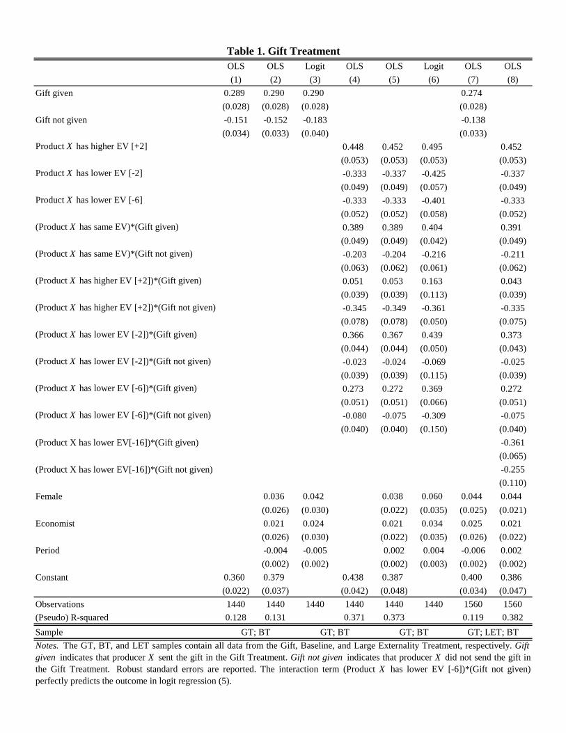
OLS OLS Logit OLS OLS Logit OLS OLS(1) (2) (3) (4) (5) (6) (7) (8)

Gift given 0.289 0.290 0.290 0.274(0.028) (0.028) (0.028) (0.028)

Gift not given -0.151 -0.152 -0.183 -0.138(0.034) (0.033) (0.040) (0.033)

Product X has higher EV [+2] 0.448 0.452 0.495 0.452(0.053) (0.053) (0.053) (0.053)

Product X has lower EV [-2] -0.333 -0.337 -0.425 -0.337(0.049) (0.049) (0.057) (0.049)

Product X has lower EV [-6] -0.333 -0.333 -0.401 -0.333(0.052) (0.052) (0.058) (0.052)

(Product X has same EV)*(Gift given) 0.389 0.389 0.404 0.391(0.049) (0.049) (0.042) (0.049)

(Product X has same EV)*(Gift not given) -0.203 -0.204 -0.216 -0.211(0.063) (0.062) (0.061) (0.062)

(Product X has higher EV [+2])*(Gift given) 0.051 0.053 0.163 0.043(0.039) (0.039) (0.113) (0.039)

(Product X has higher EV [+2])*(Gift not given) -0.345 -0.349 -0.361 -0.335(0.078) (0.078) (0.050) (0.075)

(Product X has lower EV [-2])*(Gift given) 0.366 0.367 0.439 0.373(0.044) (0.044) (0.050) (0.043)

(Product X has lower EV [-2])*(Gift not given) -0.023 -0.024 -0.069 -0.025(0.039) (0.039) (0.115) (0.039)

(Product X has lower EV [-6])*(Gift given) 0.273 0.272 0.369 0.272(0.051) (0.051) (0.066) (0.051)

(Product X has lower EV [-6])*(Gift not given) -0.080 -0.075 -0.309 -0.075(0.040) (0.040) (0.150) (0.040)

(Product X has lower EV[-16])*(Gift given) -0.361(0.065)

(Product X has lower EV[-16])*(Gift not given) -0.255(0.110)

Female 0.036 0.042 0.038 0.060 0.044 0.044(0.026) (0.030) (0.022) (0.035) (0.025) (0.021)

Economist 0.021 0.024 0.021 0.034 0.025 0.021(0.026) (0.030) (0.022) (0.035) (0.026) (0.022)

Period -0.004 -0.005 0.002 0.004 -0.006 0.002(0.002) (0.002) (0.002) (0.003) (0.002) (0.002)

Constant 0.360 0.379 0.438 0.387 0.400 0.386(0.022) (0.037) (0.042) (0.048) (0.034) (0.047)

Observations 1440 1440 1440 1440 1440 1440 1560 1560(Pseudo) R-squared 0.128 0.131 0.371 0.373 0.119 0.382SampleNotes. The GT, BT, and LET samples contain all data from the Gift, Baseline, and Large Externality Treatment, respectively. Gift given indicates that producer X sent the gift in the Gift Treatment. Gift not given indicates that producer X did not send the gift inthe Gift Treatment. Robust standard errors are reported. The interaction term (Product X has lower EV [-6])*(Gift not given)perfectly predicts the outcome in logit regression (5).

Table 1. Gift Treatment

GT; BT GT; BT GT; BT GT; LET; BT

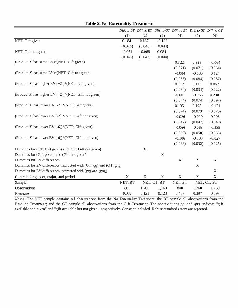
Diff. to BT Diff. to BT Diff. to GT Diff. to BT Diff. to BT Diff. to GT(1) (2) (3) (4) (5) (6)

NET: Gift given 0.184 0.187 -0.103(0.046) (0.046) (0.044)

NET: Gift not given -0.071 -0.068 0.084(0.043) (0.042) (0.044)

(Product X has same EV)*(NET: Gift given) 0.322 0.325 -0.064(0.071) (0.071) (0.064)

(Product X has same EV)*(NET: Gift not given) -0.084 -0.080 0.124(0.085) (0.084) (0.087)

(Product X has higher EV [+2])*(NET: Gift given) 0.112 0.115 0.062(0.034) (0.034) (0.022)

(Product X has higher EV [+2])*(NET: Gift not given) -0.061 -0.058 0.290(0.074) (0.074) (0.097)

(Product X has lower EV [-2])*(NET: Gift given) 0.195 0.195 -0.171(0.074) (0.073) (0.076)

(Product X has lower EV [-2])*(NET: Gift not given) -0.026 -0.020 0.003(0.047) (0.047) (0.049)

(Product X has lower EV [-6])*(NET: Gift given) -0.066 -0.063 -0.335(0.050) (0.050) (0.055)

(Product X has lower EV [-6])*(NET: Gift not given) -0.106 -0.103 -0.027(0.033) (0.032) (0.025)

Dummies for (GT: Gift given) and (GT: Gift not given) XDummies for (Gift given) and (Gift not given) XDummies for EV differences X X XDummies for EV differences interacted with (GT: gg) and (GT: gng) XDummies for EV differences interacted with (gg) and (gng) XControls for gender, major, and period X X X X X XSample NET, BT NET, BTObservations 800 1,760 1,760 800 1,760 1,760R-square 0.037 0.123 0.123 0.437 0.397 0.397

Table 2. No Externality Treatment

Notes. The NET sample contains all observations from the No Externality Treatment; the BT sample all observations from theBaseline Treatment; and the GT sample all observations from the Gift Treatment. The abbreviations gg and gng indicate "giftavailable and given" and "gift available but not given," respectively. Constant included. Robust standard errors are reported.

NET, GT, BT NET, GT, BT

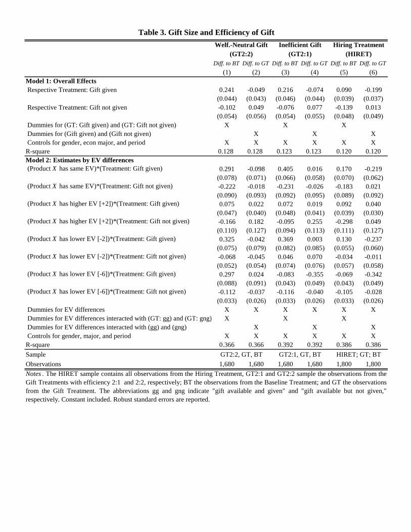
Diff. to BT Diff. to GT Diff. to BT Diff. to GT Diff. to BT Diff. to GT(1) (2) (3) (4) (5) (6)

Model 1: Overall Effects Respective Treatment: Gift given 0.241 -0.049 0.216 -0.074 0.090 -0.199

(0.044) (0.043) (0.046) (0.044) (0.039) (0.037) Respective Treatment: Gift not given -0.102 0.049 -0.076 0.077 -0.139 0.013

(0.054) (0.056) (0.054) (0.055) (0.048) (0.049) Dummies for (GT: Gift given) and (GT: Gift not given) X X X Dummies for (Gift given) and (Gift not given) X X X Controls for gender, econ major, and period X X X X X XR-square 0.128 0.128 0.123 0.123 0.120 0.120Model 2: Estimates by EV differences (Product X has same EV)*(Treatment: Gift given) 0.291 -0.098 0.405 0.016 0.170 -0.219

(0.078) (0.071) (0.066) (0.058) (0.070) (0.062) (Product X has same EV)*(Treatment: Gift not given) -0.222 -0.018 -0.231 -0.026 -0.183 0.021

(0.090) (0.093) (0.092) (0.095) (0.089) (0.092) (Product X has higher EV [+2])*(Treatment: Gift given) 0.075 0.022 0.072 0.019 0.092 0.040

(0.047) (0.040) (0.048) (0.041) (0.039) (0.030) (Product X has higher EV [+2])*(Treatment: Gift not given) -0.166 0.182 -0.095 0.255 -0.298 0.049

(0.110) (0.127) (0.094) (0.113) (0.111) (0.127) (Product X has lower EV [-2])*(Treatment: Gift given) 0.325 -0.042 0.369 0.003 0.130 -0.237

(0.075) (0.079) (0.082) (0.085) (0.055) (0.060) (Product X has lower EV [-2])*(Treatment: Gift not given) -0.068 -0.045 0.046 0.070 -0.034 -0.011

(0.052) (0.054) (0.074) (0.076) (0.057) (0.058) (Product X has lower EV [-6])*(Treatment: Gift given) 0.297 0.024 -0.083 -0.355 -0.069 -0.342

(0.088) (0.091) (0.043) (0.049) (0.043) (0.049) (Product X has lower EV [-6])*(Treatment: Gift not given) -0.112 -0.037 -0.116 -0.040 -0.105 -0.028

(0.033) (0.026) (0.033) (0.026) (0.033) (0.026) Dummies for EV differences X X X X X X Dummies for EV differences interacted with (GT: gg) and (GT: gng) X X X Dummies for EV differences interacted with (gg) and (gng) X X X Controls for gender, major, and period X X X X X XR-square 0.366 0.366 0.392 0.392 0.386 0.386SampleObservations 1,680 1,680 1,680 1,680 1,800 1,800

(HIRET)

Notes . The HIRET sample contains all observations from the Hiring Treatment, GT2:1 and GT2:2 sample the observations from theGift Treatments with efficiency 2:1 and 2:2, respectively; BT the observations from the Baseline Treatment; and GT the observationsfrom the Gift Treatment. The abbreviations gg and gng indicate "gift available and given" and "gift available but not given,"respectively. Constant included. Robust standard errors are reported.

Hiring Treatment

Table 3. Gift Size and Efficiency of GiftInefficient GiftWelf.-Neutral Gift

GT2:2, GT, BT GT2:1, GT, BT HIRET; GT; BT

(GT2:2) (GT2:1)

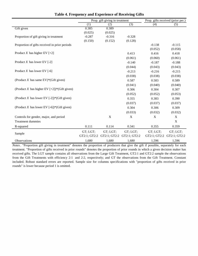
(1) (2) (3) (4) (5)Gift given 0.385 0.389

(0.025) (0.025)Proportion of gift giving in treatment -0.287 -0.316 -0.328

(0.150) (0.152) (0.128)Proportion of gifts received in prior periods -0.138 -0.115

(0.052) (0.058)Product X has higher EV [+2] 0.413 0.416 0.418

(0.061) (0.060) (0.061)Product X has lower EV [-2] -0.140 -0.187 -0.188

(0.044) (0.043) (0.043)Product X has lower EV [-6] -0.213 -0.216 -0.215

(0.038) (0.038) (0.038)(Product X has same EV)*(Gift given) 0.587 0.583 0.589

(0.041) (0.040) (0.040)(Product X has higher EV [+2])*(Gift given) 0.306 0.304 0.307

(0.052) (0.052) (0.053)(Product X has lower EV [-2])*(Gift given) 0.355 0.383 0.390

(0.037) (0.037) (0.037)(Product X has lower EV [-6])*(Gift given) 0.304 0.306 0.309

(0.033) (0.032) (0.032)Controls for gender, major, and period X X X XTreatment dummies XR-squared 0.111 0.114 0.341 0.355 0.359

Sample GT; LGT; GT2:1; GT2:2

GT; LGT; GT2:1; GT2:2

GT; LGT; GT2:1; GT2:2

GT; LGT; GT2:1; GT2:2

GT; LGT; GT2:1; GT2:2

Observations 1,680 1,680 1,680 1,596 1,596

Table 4. Frequency and Experience of Receiving GiftsProp. gift giving in treatment Prop. gifts received (prior per.)

Notes . "Proportion gift giving in treatment" denotes the proportion of producers that give the gift if possible, separately for eachtreatment. "Proportion of gifts received in prior rounds" denotes the proportion of prior rounds in which a given decision maker hasreceived gifts. The LGT sample contains all observations from the Large Gift Treatment, GT2:1 and GT2:2 sample the observationsfrom the Gift Treatments with efficiency 2:1 and 2:2, respectively; and GT the observations from the Gift Treatment. Constantincluded. Robust standard errors are reported. Sample size for columns specifications with "proportion of gifts received in priorrounds" is lower because period 1 is omitted.

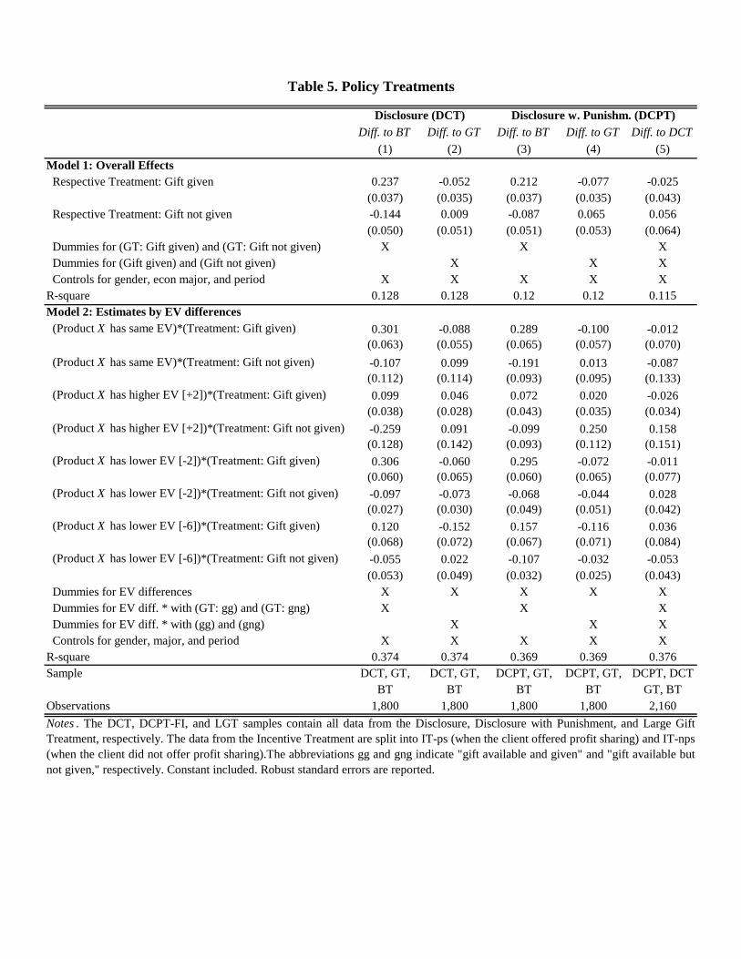
Diff. to BT Diff. to GT Diff. to BT Diff. to GT Diff. to DCT(1) (2) (3) (4) (5)

Model 1: Overall Effects Respective Treatment: Gift given 0.237 -0.052 0.212 -0.077 -0.025

(0.037) (0.035) (0.037) (0.035) (0.043) Respective Treatment: Gift not given -0.144 0.009 -0.087 0.065 0.056

(0.050) (0.051) (0.051) (0.053) (0.064) Dummies for (GT: Gift given) and (GT: Gift not given) X X X Dummies for (Gift given) and (Gift not given) X X X Controls for gender, econ major, and period X X X X XR-square 0.128 0.128 0.12 0.12 0.115Model 2: Estimates by EV differences (Product X has same EV)*(Treatment: Gift given) 0.301 -0.088 0.289 -0.100 -0.012

(0.063) (0.055) (0.065) (0.057) (0.070) (Product X has same EV)*(Treatment: Gift not given) -0.107 0.099 -0.191 0.013 -0.087

(0.112) (0.114) (0.093) (0.095) (0.133) (Product X has higher EV [+2])*(Treatment: Gift given) 0.099 0.046 0.072 0.020 -0.026

(0.038) (0.028) (0.043) (0.035) (0.034) (Product X has higher EV [+2])*(Treatment: Gift not given) -0.259 0.091 -0.099 0.250 0.158

(0.128) (0.142) (0.093) (0.112) (0.151) (Product X has lower EV [-2])*(Treatment: Gift given) 0.306 -0.060 0.295 -0.072 -0.011

(0.060) (0.065) (0.060) (0.065) (0.077) (Product X has lower EV [-2])*(Treatment: Gift not given) -0.097 -0.073 -0.068 -0.044 0.028

(0.027) (0.030) (0.049) (0.051) (0.042) (Product X has lower EV [-6])*(Treatment: Gift given) 0.120 -0.152 0.157 -0.116 0.036

(0.068) (0.072) (0.067) (0.071) (0.084) (Product X has lower EV [-6])*(Treatment: Gift not given) -0.055 0.022 -0.107 -0.032 -0.053

(0.053) (0.049) (0.032) (0.025) (0.043) Dummies for EV differences X X X X X Dummies for EV diff. * with (GT: gg) and (GT: gng) X X X Dummies for EV diff. * with (gg) and (gng) X X X Controls for gender, major, and period X X X X XR-square 0.374 0.374 0.369 0.369 0.376Sample DCT, GT, DCT, GT, DCPT, GT, DCPT, GT, DCPT, DCT

BT BT BT BT GT, BTObservations 1,800 1,800 1,800 1,800 2,160

Table 5. Policy Treatments

Notes . The DCT, DCPT-FI, and LGT samples contain all data from the Disclosure, Disclosure with Punishment, and Large GiftTreatment, respectively. The data from the Incentive Treatment are split into IT-ps (when the client offered profit sharing) and IT-nps(when the client did not offer profit sharing).The abbreviations gg and gng indicate "gift available and given" and "gift available butnot given," respectively. Constant included. Robust standard errors are reported.

Disclosure (DCT) Disclosure w. Punishm. (DCPT)

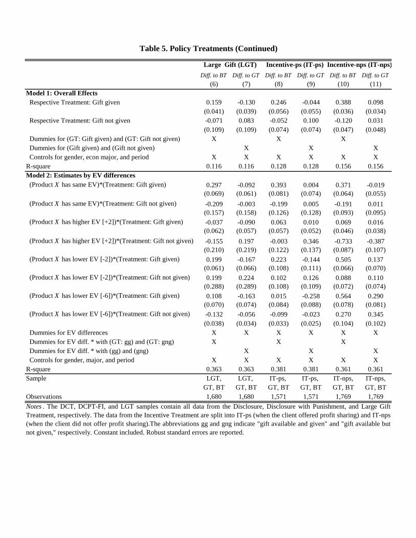
Diff. to BT Diff. to GT Diff. to BT Diff. to GT Diff. to BT Diff. to GT(6) (7) (8) (9) (10) (11)

Model 1: Overall Effects Respective Treatment: Gift given 0.159 -0.130 0.246 -0.044 0.388 0.098

(0.041) (0.039) (0.056) (0.055) (0.036) (0.034) Respective Treatment: Gift not given -0.071 0.083 -0.052 0.100 -0.120 0.031

(0.109) (0.109) (0.074) (0.074) (0.047) (0.048) Dummies for (GT: Gift given) and (GT: Gift not given) X X X Dummies for (Gift given) and (Gift not given) X X X Controls for gender, econ major, and period X X X X X XR-square 0.116 0.116 0.128 0.128 0.156 0.156Model 2: Estimates by EV differences (Product X has same EV)*(Treatment: Gift given) 0.297 -0.092 0.393 0.004 0.371 -0.019

(0.069) (0.061) (0.081) (0.074) (0.064) (0.055) (Product X has same EV)*(Treatment: Gift not given) -0.209 -0.003 -0.199 0.005 -0.191 0.011

(0.157) (0.158) (0.126) (0.128) (0.093) (0.095) (Product X has higher EV [+2])*(Treatment: Gift given) -0.037 -0.090 0.063 0.010 0.069 0.016

(0.062) (0.057) (0.057) (0.052) (0.046) (0.038) (Product X has higher EV [+2])*(Treatment: Gift not given) -0.155 0.197 -0.003 0.346 -0.733 -0.387

(0.210) (0.219) (0.122) (0.137) (0.087) (0.107) (Product X has lower EV [-2])*(Treatment: Gift given) 0.199 -0.167 0.223 -0.144 0.505 0.137

(0.061) (0.066) (0.108) (0.111) (0.066) (0.070) (Product X has lower EV [-2])*(Treatment: Gift not given) 0.199 0.224 0.102 0.126 0.088 0.110

(0.288) (0.289) (0.108) (0.109) (0.072) (0.074) (Product X has lower EV [-6])*(Treatment: Gift given) 0.108 -0.163 0.015 -0.258 0.564 0.290

(0.070) (0.074) (0.084) (0.088) (0.078) (0.081) (Product X has lower EV [-6])*(Treatment: Gift not given) -0.132 -0.056 -0.099 -0.023 0.270 0.345

(0.038) (0.034) (0.033) (0.025) (0.104) (0.102) Dummies for EV differences X X X X X X Dummies for EV diff. * with (GT: gg) and (GT: gng) X X X Dummies for EV diff. * with (gg) and (gng) X X X Controls for gender, major, and period X X X X X XR-square 0.363 0.363 0.381 0.381 0.361 0.361Sample LGT, LGT, IT-ps, IT-ps, IT-nps, IT-nps,

GT, BT GT, BT GT, BT GT, BT GT, BT GT, BTObservations 1,680 1,680 1,571 1,571 1,769 1,769Notes . The DCT, DCPT-FI, and LGT samples contain all data from the Disclosure, Disclosure with Punishment, and Large GiftTreatment, respectively. The data from the Incentive Treatment are split into IT-ps (when the client offered profit sharing) and IT-nps(when the client did not offer profit sharing).The abbreviations gg and gng indicate "gift available and given" and "gift available butnot given," respectively. Constant included. Robust standard errors are reported.

Table 5. Policy Treatments (Continued)

Large Gift (LGT) Incentive-ps (IT-ps) Incentive-nps (IT-nps)