1

Simulation of the Middle Miocene Climate Optimum

By

You, Y.1,2,*, M. Huber3, D. Müller2, C.J. Poulsen4, J. Ribbe5

1University of Sydney Institute of Marine Science, University of Sydney, NSW 2006, Australia

2School of Earth Sciences, University of Sydney, NSW 2006, Australia

3Dept of Earth and Atmospheric Sciences, Purdue University, West Lafayette, IN 47907, USA

4Dept of Geological Sciences, University of Michigan, Ann Arbor, MI 48109

5Dept of Biological and Physical Sciences, University of Southern Queensland, Toowoomba, Queensland

4350, Australia

*Corresponding author, Phone: 61-2-93512004, Fax: 61-2-93510184, Email: you@geosci.usyd.edu.au

Submitted to GRL

(Revised in Sydney, Dec 2008)

2

ABSTRACT

Proxy data constraining land and ocean surface paleo-temperatures indicate that the Middle

Miocene Climate Optimum (MMCO), a global warming event at ~15 Ma, had a global annual

mean surface temperature of 18.4°C, about 3°C higher than present and equivalent to the

warming predicted for the next century. We apply the latest National Center for Atmospheric

Research (NCAR) Community Atmosphere Model CAM3.1 and Land Model CLM3.0 coupled

to a slab ocean to examine sensitivity of MMCO climate to varying ocean heat fluxes derived

from paleo sea surface temperatures (SSTs) and atmospheric carbon dioxide concentrations,

using detailed reconstructions of Middle Miocene boundary conditions including

paleogeography, elevation, vegetation and surface temperatures. Our model suggests that to

maintain MMCO warmth consistent with proxy data, the required atmospheric CO2

concentration is about 460-580 ppmv, narrowed from the most recent estimate of 300-600 ppmv.

1. INTRODUCTION

The Middle Miocene Climate Optimum (MMCO) occurred at about 15 Ma and represents a

geologically recent warming event unrelated to human activity that may mirror future climate

change in terms of the average global surface temperature increase. Flower and Kennett [1994]

estimate that the MMCO was associated with a mid-latitude warming of about 6°C relative to the

present. However, the cause of the MMCO warming and the role and scale of atmospheric

carbon dioxide (CO2) is vigorously debated. Estimates of Middle Miocene paleo-CO2 range from

glacial levels to nearly twice the modern value. On the basis of paleosol 13

C, Cerling [1991]

estimates a mean mid-Miocene atmospheric CO2 concentration of 700 ppmv. Using stomatal

indices from fossil leaves, Royer et al. [2000] and Kürschner et al. [2008] obtain intermediate

values ranging from somewhat less than modern (307-316 ppmv) to higher-than-modern (500

ppmv) CO2 levels. In contrast, marine CO2 proxy records indicate much lower values. Pagani et

al. [1999] calculate CO2 levels of 180-290 ppmv, low values which were confirmed by Pearson

and Palmer [2000]. The low CO2 estimates suggest that CO2 and surface temperature were not

3

linked during the MMCO, and raises the possibility of a CO2-temperature decoupling during

other times in Earth history.

To date the warmth of the MMCO under low CO2 levels has not been reproduced by climate

models. Modeling of the MMCO has proven to be extremely difficult due to a lack of detailed

global boundary and initial conditions, sparse proxy data, and disparate CO2 concentrations.

Here we use the latest NCAR Atmosphere Model CAM3.1 and Land Model CLM3.0 coupled to

a slab ocean forced with realistic Miocene boundary conditions, including vegetation, elevation,

SST forcing and calculated ocean heat fluxes based on proxies, and orbital parameters, to narrow

the likely range of MMCO atmospheric CO2 concentrations.

2. DATA AND METHODS

The SSTs based on oxygen stable isotopes δ18

O for the MMCO are scarce. Moreover, the

distribution of proxy SSTs is not uniform, but skewed toward the low latitudes of the northern

hemisphere. A summary of all available paleo-SSTs demonstrates a very large scatter of tropical

SST's between about 15° and 30°C. A Gaussian best-fit to the data ranges from 0-5°C at high

latitudes to about 23°C at low latitudes, nearly 5°C lower than present (see Figures 1a and 2).

The approach we take is to use reconstructed Miocene SST gradients to estimate meridional

ocean heat fluxes. This is necessary because slab ocean models do not include dynamics, and the

modern ocean heat flux may not be appropriate for Miocene [von der Heydt and Dijkstra, 2006].

First, we prescribe zonal constant SST constructed from a Gaussian best fit to all proxy data with

a lowest equator-to-pole gradient called LGRAD, equivalent to the so called “cool tropical

paradox”. Following the method of Huber et al. [2003], we then modify the LGRAD by creating

a new SST gradient using the maximum SSTs in the tropics, but modified high latitudes

temperatures to maintain the global mean SST of 20.6°C. Here we choose two modified zonal

SST profiles, one matching the present SST called MGRAD with a medium equator-to-pole

gradient and another HGRAD with equatorial SST 2-3°C higher than present [Graham, 1994].

As a result, three scenarios of initial SST forcing are specified. Monthly SSTs are calculated

based on present seasonality (see SM_JJA and SM_DJF for summer and winter in Figure 1a).

4

The models we employ are the latest NCAR CAM3.1 and CLM3.0 coupled to a slab ocean

model with a T31 resolution (~3.75°x3.75°). The CAM3.1 has 26 vertical levels and CLM3.0

includes 10 soil layers. The Miocene vegetation is based on Wolf [1985] with additional detail

for the Australian continent [Christophel, 1989]. To represent the absence of continental ice

sheets during the Miocene, both Greenland and West Antarctic elevations have been reduced and

land surface types have been modified to tundra. The East Antarctic remains ice covered with

modern elevations. Sea ice is assumed to be absent globally, given that none of the SST proxies

infer temperatures below 5°C.

Our middle Miocene paleotopography is constructed from the rotation of present day major

tectonic plates back to 15 Ma, using the plate model from Müller et al. [2008]. We apply a

maximum Tibetan Plateau elevation of 4700 m and a northern, central and southern Andes

elevation of 500, 900 and 600 m, respectively. Maximum sea level in MMCO was estimated to

have been about 100 m higher than present by Haq and Al-Qahtani [2005]; we use a conservative

sea-level increase of about 50 m. In the absence of proxy data, greenhouse gas concentrations are

set to preindustrial levels for methane (700 ppbv), nitrous oxide (275 ppbv), and

chlorofluorocarbons (0 ppbv). The solar and orbital parameters are assumed to be constant for

the middle Miocene period at 15 Ma and set to 1.368E6 W m-2

for the solar constant, 0.01492 for

eccentricity, 181.0725 for precession and 23.46185 for obliquity [Laskar et al., 2004]. The initial

CO2 concentration is 700 ppmv in each of the scenarios referred to as high (SH_700), medium

(SM_700) and low (SL_700) gradient SST forcing.

With the Miocene boundary conditions, the CAM3.1 coupled with CLM3.0 is initially integrated

for 30 years with a data ocean model (DOM), which simply reads and interpolates the specified

SST. This is necessary for the calculation of monthly ocean heat fluxes (i.e., Qflux), which are

used in the subsequent slab ocean (SOM) runs. The model run is iterated, adjusting the low and

high cloud relative humidity in CAM model code, until top-of-the-atmosphere and surface

radiative balance is achieved, at which point the model is considered to be in equilibrium. The

adjustment is necessary due to the change of initial and boundary conditions during MMCO so

that radiative energy may be slightly imbalance. The last 10 years of the DOM run are used to

5

calculate the Qflux. The CAM3.1 is then coupled with CLM3.0 and a slab ocean model (SOM),

and run for 60 model years.

In addition to our standard SH, SM, and SL cases with 700 ppmv CO2, branch runs were

completed for each SST scenario with CO2 concentrations reduced by approximately 50% to 350

and 180 ppmv. Branch runs were started from the end of our standard cases and iterated for 100

model years to attain equilibrium. In total, nine experiments were completed, three for each

scenario: SH (SH_700, SH_350 and SH_180); SM (SM_700, SM_350 and SM_180) and SL

(SL_700, SL_350 and SL_180). To compare with the Miocene model results, a present day SOM

run called MODERN is also carried out with CO2 355 ppmv and present boundary and initial

conditions. In addition, a present day SOM experiment was run with Miocene orbital parameters

to examine their effect on global surface temperatures. The mean of the last 10 years of each

model run is presented here for analysis.

3. RESULTS

The simulated SSTs for the three scenarios, SH_700, SM_700 and SL_700, are compared with

present and proxy SSTs (Figure 1a). The SL SST (short dashed line) most closely matches proxy

SST, as determined by a Gaussian best fit. In this simulation, low-latitude SSTs are about 22°C.

Polar SSTs are more than 10°C higher than present with an asymmetrical meridional distribution,

a minimum of 5°C in Arctic and 0.5°C at Antarctica. The OHT of these simulations is examined

in Figure 1b. Although the SL simulation best matches the proxy SST, the OHT is unrealistically

large, approximately twice the modern heat transport, a result that is unlikely given current

coupled modeling results [von der Heydt and Dijkstra, 2006]. This result indicates that to get a

very low temperature gradient, and temperatures that match the magnitudes of proxy SST, high

CO2 in addition to high OHT is necessary [Barron and Peterson, 1989; Huber and Sloan, 2001;

Shellito, et al., 2003; Sloan and Rea, 1995]. In contrast, the simulated OHT for SH and SM (in

thin and thick solid lines) is similar to present. The SH has a peak tropical SST of about 31°C

which is about 3°C higher than the present value of about 28°C. The SM tropical SST maximum

is about 29°C only slightly higher than present.

6

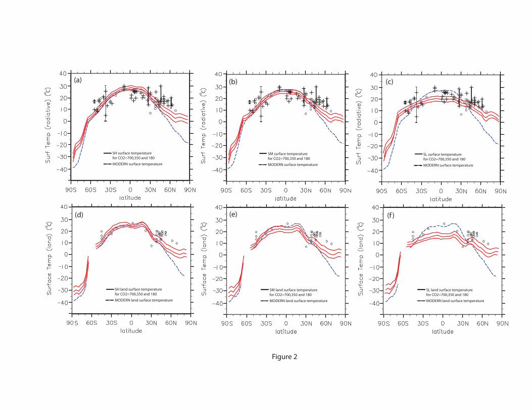
The simulated annual global mean surface temperature (upper panel) and land-only surface

temperature (lower panel) are presented in Figure 2, and compared with the present value

(dashed line) and proxies for Miocene SST (in cross) and land (in open circle). In each scenario,

the simulated surface temperature decreases by about 2° and 4°C, respectively, with the rough

50% decrease in CO2. The proxy surface temperature is best simulated in the SH and SM

experiments with CO2 concentrations of 350 and 700 ppmv, respectively, as their global mean

surface temperature is closest to the proxy mean temperature (see Figures 2a, b, d, and e). This

comparison is further examined in Figure 3. In contrast, simulated surface temperature in the SL

cases is lower than marine and terrestrial proxies (Figures 2c and 2f), although SST is best

matched in the first case above.

In Figure 3, simulated global annual mean surface temperature is compared to the atmospheric

CO2 concentrations. The global annual mean proxy surface temperature, including ocean and

terrestrial data, is 18.4°C, about 3°C higher than that for the present-day simulation (asterisk).

This represents the first assessment of the MMCO with a large distribution of proxy data used to

estimate a global average temperature. Since most proxy data are found in mid latitudes, the

simulated result gives more weight to those latitudes than high and low latitudes. The global

average proxy temperature likely has an uncertainty of at least ±1°C. Two simulations, SH_350

and SM_700, with a global mean temperature 17.8°C and 19.0°C, fall within this error range

(about 2.3°C and 3.5°C higher than present, respectively). This is close to the difference between

the proxy and present simulation (2.9ºC). Interestingly, SH_350 compares well because its land

surface temperature (16.2°C) is almost the same as that derived from proxy data (16.1°C).

Likewise, SM_700 has a mean SST of 20.5°C which is about the same as the proxy-derived SST

(20.6°C). The SL simulated mean SST's (in triangle, also see Figure 2) are generally too low.

Although SL_700 reaches the lower error bar (-1ºC), the unrealistic OHT and poor comparison

with proxy data, especially the land surface data (Figures 2c and 2f), render it unacceptable.

However, even under relatively low CO2, the mean surface temperatures are substantially higher

than present with a suitable SST forcing. The effect of MMCO orbital parameters on global

mean surface temperature with respect to modern orbital parameters is small (-0.1°C).

7

4. DISCUSSION

The issue of anomalously low Miocene tropical SST‟s derived from proxy data has been debated

for some time. However a bias in proxy data may exist and is discussed here. The scattered

tropical SST proxies are perhaps sampled through the same species of foraminifer shells, but

under different conditions of diagenesis. Using well conserved foraminifer shells extracted from

impermeable clay-rich sediments, Pearson et al. [2001] obtained tropical SST's of at least 28°-

32°C in the Late Cretaceous and Eocene epochs, much higher than the 15°-23°C range estimated

previously. Poulsen et al. [1999] and Huber [2008] discuss a number of issues that may cause

low tropical SST estimates for past greenhouse intervals, associated with effects of diagenesis

and assumptions of deep water properties for ancient seawater. A similar bias might apply to the

MMCO proxy data. Another possibility is that planktonic foraminiferal preferentially grow

during winter, thus recording lower seasonal temperature rather than mean-annual temperature

[Kobashi et al., 2001]. These factors are sufficient to explain the low tropical SST from proxy

data (Figure 1a). In past model simulations, the “cool tropical paradox” and high subpolar SST's

from proxies could not be reproduced [Huber and Sloan, 2001]. Many studies thus tend to agree

that for most of the Tertiary the paleotropical SST should not differ from present by more than

about 2°-3°C [Adams et al., 1990; Graham, 1994].

Except for some local bias especially in the northern mid-to-high latitudes, our model

simulations are validated by a global averaged proxy surface temperature which has reduced the

probable bias to a minimum. However, the model-proxy-disagreement in part of the northern

hemisphere latitudes may be due to the initial low meridional SST forcing input resulting in the

simulated SST bias in mid-to-high latitudes in Figure 1a. On the other hand, the present-based-

model may be less capable of simulating the asymmetrical meridional distribution of proxy

surface temperature but more study is obviously needed in future. With Gaussian best fitting

method of the SST proxy, our model fails to correctly simulate the OHT and surface

temperatures. Successful simulations are achieved when the regression of the SST proxy is

modified to match the maximum tropical temperatures while leaving the global mean SST value

unchanged. This is done under the pretense that partial tropical Miocene proxies do not provide

faithful temperature estimates. Our best simulations narrow the possible mid-Miocene

8

atmospheric CO2 concentration from 300-600 ppmv to 460-580 ppmv. However, our simulation

still lacks a dynamic ocean model which may further improve paleo-atmospheric CO2

simulations. Due to the limited space here we have not addressed other mechanisms to cause the

MMCO warming such as the changes in global albedo, vegetation and altimetry which will be

sought in future study.

Acknowledgments

The project is supported by an Australian Research Council Discovery grant. We thank Nicholas

Herold for providing the land proxy data. The model simulations were carried out on the APAC

supercomputer in Canberra under a merit allocation scheme. Discussions with Bette Otto-

Bliesner and Karen Bice are helpful. This work is initiated during first author‟s visit to Purdue

University.

9

6. References

Adams, C.G., D.E. Lee and B.R. Rosen (1990), Conflicting isotopic and biotic evidence for

tropical sea-surface temperatures during the Tertiary, Palaeogeography, Palaeoclimatology,

Palaeoecology, 77, 289-313.

Barron, E.J. and W.H. Peterson (1989), Model simulation of the Cretaceous ocean circulation,

Science, 244, 684-686.

Bojar, A. V., H. Hiden, A. Fenninger and F. Neubauer (2005), Middle Miocene temperature

changes in the central paratethys: Relations with the east Antarctica ice sheet development,

Short-papers-IV South American Symposium on Isotope Geology, 328-330.

Cerling, T. E. (1991), Carbon dioxide in the atmosphere: evidence from Cenozoic and Mesozoic

paleosols, American Journal of Science, 291, 377-400.

Christophel, D.C. (1989), Evolution of the Australian flora through the Tertiary: Plant

Systematics and Evolution, v. 162, p. 63-78.

Devereux, I. (1967), Oxygen isotope paleo-temperature measurements on New Zealand Tertiary

fossils, New Zealand Journal of Science, 10, 988-1011.

Flower, B. P., and J. P. Kennett (1994), The Middle Miocene climatic transition: East Antarctic

ice sheet development, deep ocean circulation and global carbon cycling, Palaeogeography,

Palaeoclimatology, Palaeoecology, 108, 537-555.

Flower, B.P. (1999), Warming without high CO2? Nature, 399, 313-314.

Graham, A. (1994), Neotropical Eocene coastal floras and 18

O/16

O-estimated warmer vs. cooler

equatorial waters, American Journal of Botany, 81, 301-306.

Gonera, M., T. M. Peryt and T. Durakiewicz (2000), Biostratigraphical and palaeoenvironmental

implications of isotopic studies (18

O, 13

C) of middle Miocene (Badenian) foraminifers in the

Central Paratethys, Terra Nova, 12(5), 231-238.

Haq, B.U. and A.M. Al-Qahtani (2005), Phanerozoic cycles of sea-level change on the Arabian

Platform. GeoArabia, 10, 127-160.

Huber, M. (2008), A hotter greenhouse? Science, 321, 353-354, doi:10.1126/science1161170.

10

Huber, M. and L.C. Sloan (2001), Heat transport, deep waters, and thermal gradients: Coupled

simulation of an Eocene greenhouse climate, Geophysical Research Letters, 28, 3481-3484.

Huber, M., L.C. Sloan and C. Shellito (2003), Early Paleogene oceans and climate: A fully

coupled modeling approach using the NCAR CCSM, in Wing, S.L., Gingerich, P.D.,

Schmitz, B. and Thomas, E., eds., Causes and Consequences of Globally Warm Climates in

the Early Paleogene: Boulder, Colorado, Geological Society of America Special Paper 369, p.

25-47.

Jenkins, D. G. (1968), Variations in the number of species and subspecies of planktic

foraminiferida as an indicator of New Zealand Cenozoic paleotemperatures,

Palaeogeography, Palaeoclimatology, palaeoecology, 5, 309-313.

Kershaw, A. P. (1997), A bioclimatic analysis of early to middle Miocene brown coal floras,

Latrobe valley, south-eastern Australia, Australian Journal of Botany, 45, 373-387.

Kobashi, T., E.L. Grossman, T.E. Yancey and D.T. Dockery, III (2001), Reevaluation of

conflicting Eocene tropical temperature estimates: Molluskan oxygen isotope evidence for

warm low latitudes, Geology, 29, 983-986.

Kürschner, W.M., Z. Kvaček and D.L. Dilcher (2008), The impact of Miocene atmospheric

carbon dioxide fluctuations on climate and the evolution of terrestrial ecosystems,

Proceedings of the National Academy of Sciences, 105, 449-453.

Laskar, J., P. Robutel, F. Joutel, M. Gastineau, A.C.M. Correia and B. Levrard (2004), A long-

term numerical solution for the insolation quantities of the Earth, Astronomy and

Astrophysics, 428, 261-285.

Müller, R.D., M. Sdrolias, C. Gaina, B. Steinberger and C. Heine (2008), Long-term sea level

fluctuations driven by ocean basin dynamics, Science, 319, 1357-1362.

Nikolaev, S. D., N. S. Oskina, N. S. Blyum and N. V. Bubenshchikova (1998), Neogen-

Quaternary variations of the „pole-equator‟ temperature gradient of the surface oceanic

waters in the North Atlantic and North Pacific, Global and Planetary Change, 18, 85-111.

11

Oleinik, A. E. (2001), Biogeographic and stable isotope evidence for middle Miocene warming

in the high-latitude North Pacific, GSA Annual Meeting, Boston, Massachusetts, abstract,

paper no. 159-0.

Pagani, M., M.A. Arthur and K.H. Freeman (1999), Miocene evolution of atmospheric carbon

dioxide, Paleoceanography, 14, 273-292.

Pearson, P. N., and M. R. Palmer (2000), Atmospheric carbon dioxide concentrations over the

past 60 million years, Nature, 406, 695-699.

Pearson, P.N., P.W. Ditchfield, J. Singano, K.G. Harcourt-Brown, C.J. Nicholas, R.K. Olsson,

N.J. Shackleton and M.A. Hall (2001), Warm tropical sea surface temperatures in the Late

Cretaceous and Eocene epochs, Nature, 413, 481-470.

Poulsen, C.J., E.J. Barron, W.H. Peterson and P.A. Wilson (1999), A reinterpretation of mid-

Cretaceous shallow marine temperatures through model-data comparison, Paleoceanography,

14, 679-697.

Royer, D. L., S.L. Wing, D.J. Beerling, D.W. Jolley, P.L. Koch, L.J. Hickey and R.A. Berner

(2001), Paleobotanical Evidence for Near Present-Day Levels of Atmospheric CO2 During

Part of the Tertiary, Science, 292, 2310-2313.

Savin, S. M., R. G. Douglas and F. G. Stehli (1975), Tertiary marine paleotemperatures,

Geological Society of Amrica Bulletin, 86, 1499-1510.

Savin, S. M. (1977), The history of the earth‟s surface temperature during the past 100 million

years, Annual Review of Earth and Planetary Sciences, 5, 319-355.

Shellito, C.J., L.C. Sloan and M. Huber (2003), Climate model sensitivity to atmospheric CO2

levels in the Early Middle Paleogene, Paaleogeography, Palaeoclimatology, Palaeoecology,

193, 113-123.

Shevenell, A. E., J. P. Kennett and D. W. Lea (2004), Middle Miocene Southern Ocean cooling

and Antarctic cryosphere expansion, Science, 305 (1766), doi:10.1126/science.1100061,

p.1766-1770.

12

Steppuhn, A., A. Micheels, A.A. Bruch, D. Uhl, T. Utescher and V. Mosbrugger (2007), The

sensitivity of ECHAM4/ML to a double CO2 scenario for the Late Miocene and the

comparison to terrestrial proxy data, Global and Planetary Change, 57, 189-212.

Stewart, D. R. M., P. N. Pearson, P. W. Ditchfield and J. M. Singano (2004), Miocene tropical

Indian Ocean temperatures: evidence from three exceptionally preserved foraminiferal

assemblages from Tanzania, Journal of African Earth Sciences, 40, 173-190.

Van der Smissen, J. H. and J. Rullkötter (1996), Organofacies variations in sediments from the

central slope and rise of the New Jersey continental margin (sites 903 and 905), Proceedings

of the Ocean Drilling Program, Scientific Results, 150, 329-344.

Von der Heydt, A., and H.A. Dijkstra (2006), Effect of ocean gateways on the global ocean

circulation in the late Oligocene and early Miocene, Paleoceanography, 21, PA1011,

doi:10.1029/2005PA001149.

Wolfe, J.A. (1985), Distribution of major vegetational types during the Tertiary, Geophysical

Monograph, 32, 357-375.

13

7. Figure captions

Figure 1. Zonal mean of (a) the simulated annual mean sea surface temperature (°C) for the

scenarios SH (thin solid line), SM (thick solid line) and SL (short dashed line), compared with

present (MODERN) (dashed line) and Miocene SST proxy (“+”): 1. Shevenell et al. (2004), 2.

Kershaw (1997), 3. Pagani et al. (1999), 4. Nikolaev et al. (1998), 5. Bojar et al. (2005), 6.

Gonera et al. (2002), 7. Devereux (1967), 8. Van der Smissen and Rullkötter (1996), 9. Oleinik

(2001), 10. Stewart et al. (2004), 11. Savin et al. (1975), 12. Kobashi et al. (2001), 13. Savin

(1977) and 14. Jenkins (1968); SM_JJA (thick dash dotted line) and SM_DJF (thick dashed line)

represent summer and winter SST forcing input for the DOM model run and (b) the simulated

northward ocean heat transport (PW) for the three Miocene scenarios and present.

Figure 2. Simulated zonally averaged annual mean surface temperature (upper panel) and land

only surface temperature (lower panel) for the three model scenarios SH (a and d), SM (b and e)

and SL (c and f) with CO2 concentrations from 700 ppmv to 350 and 180 ppmv, compared with

the MODERN and Miocene SST proxy (“+”) (see Figure 1 caption for references) and land

proxy (“o”) (Nicholas Herold, personal communication).

Figure 3. Simulated global annual mean surface temperature (°C) against CO2 concentrations

(ppmv) for the three Miocene scenarios, SH (“o”), SM (“+”) and SL (“^”), compared with

present day simulation (“*”) and mean proxy (thin solid line).

SHSMSLMODERN

+

+

+

+

+ +

+

++

+

+

+

+

+ +

+

+

+

+

+

+

+

+ ++

+

+

+

++

+

+

++

++

++++

++

++

+++

80S 60 40 20 0 20 40 60 80 N

5

0

-5

10

15

20

25

30

35

o o o o o o o o o

+

Latitude

An

nu

al m

ean

sea

su

rfac

e te

mp

erat

ure

( C

)o

SHSM

SLMODERN

+ SST proxy

(a)

(b)

Figure 1

SM_JJA(input)SM_DJF(input)

Co

SH surface temperaturefor CO2=700,350 and 180

MODERN surface temperature

+

+

+

+

+ +

+

++

+

+

+

+

+ +

+

+

+

+

+

+

+

+ ++

+

+

+

++

+

+

++

++

++++

++

++

+++

+

Co

SH land surface temperaturefor CO2=700,350 and 180

MODERN land surface temperature

Co

SM surface temperaturefor CO2=700,350 and 180

MODERN surface temperature

+

+

+

+

+ +

+

++

+

+

+

+

+ +

+

+

+

+

+

+

+

+ ++

+

+

+

++

+

+

++

++

++++

++

++

+++

+

Co

SM land surface temperaturefor CO2=700,350 and 180

MODERN land surface temperature

Co

SL surface temperaturefor CO2=700,350 and 180

MODERN surface temperature

+

+

+

+

+ +

+

++

+

+

+

+

+ +

+

+

+

+

+

+

+

+ ++

+

+

+

++

+

+

++

++

++++

++

++

+++

+

Co

SL land surface temperaturefor CO2=700,350 and 180

MODERN land surface temperature

(a) (b) (c)

(d) (e) (f )

Figure 2

++++++

++++

+++ +++

++++++

+++++++++

+++ +

+

+++

+++

+++++

+

+++

+++

+

+++

+

++

++ ++++++++++++ +

+

+++ +

+

++++++++

++++

+

++++

++++

+

+

+++++++

+++ ++++++++ ++

+++ +

+

++++++++

++++

100 200 300 400 500 600 700 80010

12

14

16

18

20

22

*

Glo

bal a

nnua

l mea

n su

rfac

e te

mpe

ratu

re (

C)

o

CO concentration (ppmv)2

Present

“o” : SH_180-700 ppmv“+”: SM_180-700 ppmv“^”: SL_180-700 ppmv

SM_700

SH_350

mean proxy (18.4 C)

+1 C

-1 C

o

o

o

SM

SL

SH

Figure 3

(15.5 C)o