YIELD LOCI FROM TEXTURE DATA

Textures and Microstructures, 1989, Vol. 11, pp. 23-39Reprints available directly from the publisher.Photocopying permitted by license only

1989 Gordon and Breach Science Publishers Inc.Printed in the United Kingdom

APPLICATION OF YIELD LOCI CALCULATEDFROM TEXTURE DATA

P. VAN HouTrE, K. MOLS, A. VAN BAEL and E. AERNOUDT

Department of Metallurgy and Materials Engineering, Katholieke UniversiteitLeuven, de Croylaan 2, B-3030 Leuven, Belgium

(Received February 2, 1989)

The concept of the yield locus as a means of representing the plastic anisotropy of a textured materialis remembered. It is shown how such yield loci can be used in a very general way, i.e. in fullsix-dimensional stress space. As an example of how such yield loci can actually be obtained, the seriesexpansion method based on Taylor factors is explained. It is finally shown that these six-dimensionalyield loci can be approximated by analytical expressions and under such form brought into finiteelement calculations of elasto-plastic forming processes.

KEY WORDS Yield locus, six-dimensional, Taylor model, series expansion, analytical expression.

1. INTRODUCTION

1.1 The Concept of a Yield Locus

Yield loci are tools used in the analysis of plastic forming problems. They providea means of knowing whether a uniaxial or multiaxial stress state can cause plasticdeformation in a given material. Moreover, they can be used to find the plasticstrain rate tensor that corresponds to a plastic stress by applying Hill’s MaximumWork criterion (Hill, 1950).A stress is in general described by six independent components"

Sll S22 S33 S23 "-S32 S31 --S13 and $12 $21. A condition expressing that a givenstress state Sij causes plastic flow in a given material generally takes the form"

F(So) =0 (1)For incompressible materials, the yield condition does not depend on thehydrostatic component of the stress, but only on the deviatoric stress S’. It is thenoften convenient to use expressions for the yield condition in which the S0 havebeen replaced by S. Moreover, there are only five independent deviatoric stresscomponents in such a case, which certainly is important for the analysis (VanHoutte, 1987, 1988; Lequeu et al., 1987). For reasons of clarity, we will notemphasize this aspect in the present paper.Note that for a given material, the actual form of expression (1) will depend on

the choice of the reference system used in physical space. Such condition can berepresented geometrically in a six dimensional space, of which each axiscorresponds to one of the independent stress components. Such representation iscalled a yield surface or yield locus. It evidently is impossible to visualize such six

23

24 P. VAN HOUTI’E ET AL.

dimensional yield locus in a single drawing. It is customary to represent planesections of the yield locus. Many different plane sections can be made; see forexample the cases discussed by Van Houtte (1987). Such plane section cangenerally be described as being an x, y plot in which each combination of x and ystands for the following stress state:

S xSx + ySr (2)The "basis vectors" Sx and Sy are often very simple: Sx may for example representa uniaxial stress all and Sy a uniaxial stress $22 (Figure 1). More complexexamples have been given by Van Houtte (1987).A first application of a yield locus (assuming that it is known) is to answer the

question: at what stress level will plastic yielding begin for a given stress mode U?(Figure 1, see also next section).A second application is to answer the question: what do we know about the

(plastic) strain rate tensor when we know the plastic stress? Or co.nversely, whatis the plastic stress that is associated to a given plastic strain rate E? The answerto these questions is given by the Maximum Work Criterion (Hill, 1950). Thefollowing equation can be derived from it for incompressible materials with"smooth" yield loci (without vertices)"

ij Z OF(S’kt)Sb

(3)

in which Sj are the components of the deviatoric stress tensor. Z must benon-negative but is not fixed otherwise. Only models that asume strain ratesensitivity can connect a plastic stress $ to a particular strain rate !.

1.2. The Concept of a Stress Mode

The concept of "stress mode" has been introduced by Aernoudt, Gil Sevillanoand Van Houtte (1987). It merely is a fixed direction in stress space, described by

o /SFignre 1 An example of a two-dimensional section of a yield locus. U defines a direction in suchdiagram: a "Stress mode."

YIELD LOCI CALCULATED FROM TEXTURE DATA 25

5

EFigure 2 Typical stress-strain curve. After an elastic-plastic transient, a linear part is often reached(A). This can be back-extrapolated leading to the "back-extrapolated yield stress" S,.

a "vector" U which in reality has the nature of a tensor.f In Figure 1, the plasticstress state in the direction defined by U is represented by the point A. The stress"Vector" pointing to A is given by

Sy SyU (4)in which the scalar Sy is the ratio OA/OB. It has been convened that Sy has thedimensions of a stress (force/surface) while U is dimensionless.

1.3. Back-Extrapolated YieldStresses

There may be a problem in defining the value of Sy. It will indeed depend on thevalue of the strain at which it is measured. Figure 2 shows a typical stress-straincurve. Assume that S is the level of the stress in a uniaxial tension test, and that Estands for the true strain in the tensile direction. One may conventionally define a"yield stress" at an offset, i.e. the stress for which the non-proportional part ofthe strain reaches a certain value, such as 0.01% or 0.2%. The present authorshowever prefer to use a type of "yield stress" that is relevant for the stresses thatoccur in industrial forming operations, for which the total strains nearly alwaysexceed 5%. This means that it is not necessary to consider the elastic-plastictransition region. On the other hand, the stress level will be affected by strainhardening at strain levels of 5% and more. The "back extrapolated yield stress" isoften used to overcome these problems. The true stress-strain curve sometimesreaches a linear part after the elastic-plastic transition region (A in Figure 2).This linear part is back-extrapolated to the S-axis which then gives the"back-extrapolated yield stress" Sy (at B in Figure 2).- Rigorous methods for converting deviatoric stress tensors or strain rate tensors into vectors havebeen proposed by Lequeu, Gilormini, Montheillet, Bacroix and Jonas (1987) and by Van Houtte(1988).


Aernoudt et al. (1987) proposed a method to define a back extrapolated stressfor multiaxial tests as well. S is no longer the uniaxial stress in tensile test, but is astress level such that the stress tensor is given by:

s=st (5)in which U is the stress mode. U is supposed to be constant during the test. Itmay represent a pure shear stress, a biaxial tensile stress etc. Let the tensor !represent the strain rate at a given moment during the test. A scalar/ may bedefined as follows:

/=U’ (6)/ has the dimension (time)-1 since U is dimensionless. A measure for the totalstrain is then defined as follows"

E / dt (7)

Note that these definitions are such that P., the power dissipation by unit volumecan be calculated from the scalars S and E. It is indeed seen that

P=S’=SU’,=S, (8)Scalars S and E have now been defined for multiaxial tests, which then enables tomake a plot such as Figure 2 for such tests as well. A back-extrapolated plasticstress level Sv can hence be defined, as well as the back-extrapolated yield stresstensor Sa, (Eq. (4)).These yield stresses also depend on temperature and on strain rate. These

effects will not be considered further in the present work.

1.4. Purpose of the Present Paper

These introductory remarks show, that a six dimensional yield locus based onback-extrapolated yield stresses can be conceived. It describes the basic stresslevels required for all possible uniaxial or multiaxial plastic deformation modesbeyond the elasto-plastic transition region. It does not describe effects related towork hardening. Such yield locus, when known, would nevertheless be a quiteuseful tool when analyzing complex forming operations, e.g. in FEM studies. It ishowever quite difficult to obtain for a given material. Von Mises or Hill yieldsurfaces are often used during the analysis of forming processes. Theseapproximations are often not very satisfactory for engineering materials, whichhave a crystallographic texture and correspondingly an anisotropic yield locus. Itis the purpose of this paper to show how such yield loci can be estimated fromtexture data, and how they can be used in applications such as FEM calculationsof plastic forming operations.

2. YIELD LOCI OF ANISOTROPIC MATERIALS

2.1. Isotropy vs. Anisotropy

The properties of isotropic materials do not change when an arbitrary rotation isapplied to the material, or conversely, when such rotation is applied to the


VON MiSES

21

ligure 3 n-plane section of the yield locus of:--the von Mises yield locus for isotropic materials;--the Tresca yield locus for isotropic materials;--a f.c.c, single crystal with a (001) [110] orientation.This yield locus has been obtained using the "geometrical method" described in Section 2.5.

reference system with respect to which the properties are expressed. Thus theshape of the yield locus must be independent of the choice of the referencesystem in physical space. Hence one may always choose the principal directions ofthe acting stress as reference system. The three principal stresses then are theonly stress components that are not zero, hence a three-dimensional stress spaceis sufficient for the representation of the yield locus. Figure 3 shows a c-planesectional of the von Mises and the Tresca yield loci for isotropic materials. It isworthwhile to note that the von Mises yield condition can easily be expressed as afunction of the deviatoric stresses without using the reference system of theprincipal stresses:

F(S’) (-32S’ S’)1/2 So 0 (9)in which So is the yield stress in a uniaxial tensile test.The reduction from six stress components to three principal stress components

is not possible for anisotropic materials, since the yield locus would not beindependent of the direction of the principal stresses. This has the obviousdisadvantage that one really needs six dimensions in stress space for a fullrepresentation of the yield locus. It has the advantage that one does not need toadapt the reference system in physical space to the principal directions of theacting stress.For many applications (e.g. for sheet forming, with x3 being the normal to the

sheet), one may assume that 523 "-S31 =0. This then reduces the number of

"I" A section by the plane Sll + SEE + S33 -0.For plastically incompressible materials, one can reduce the number of independent stress

components to five, see e.g. Lequeu et al. (1987) or Van Houtte (1988). Only the deviatoriccomponent of the stress (represented by $’) is relevant in such case. This will be assumed throughoutthis paper.

28 P. VAN HOUTFE ET AL.

dimensions to be considered to four, and may furthermore greatly simplify theanalysis (Van Houtte, 1987). This simplification cannot be made for three-dimensional studies of processes such as forging.

2.2. Polycrystalline Materials

Engineering materials usually consist of many tiny crystallites. The plasticdeformation of these is achieved by slip on particular slip systems, i.e. onparticular crystallographic planes and in particular directions. As a result, theyield locus of such crystallite is strongly anisotropic and may differ very muchfrom the well-known shape of the von Mises or the Tresca yield surface (Figure3).This anisotropy may be cancelled out completely if in a polycrystal all crystal

orientations are equally represented. In that case, the orientation distributionfunction f(g) that describes the texture (Bunge, 1982) is equal to 1 for all crystalorientations g. So the material will have an isotropic yield locus, but notnecessarily the "classical" von Mises-yield locus nor the Tresca-yield locus.However, for most engineering materials f(g) is not constant but depends on g.

As a result, the macroscopic yield locus will be anisotropic as well, but usually notto the same extent as the single crystal yield locus.

2.3. Calculation of Yield Loci

A method is needed that finds all possible macroscopic stresses $’ that may startplastic deformation in a given material. Mechanical tests can give someinformation, but are very time consuming and can in practice never lead to acomplete six-dimensional yield locus. So theoretical models are preferred. Fromthe outside, such models may operate in two ways:

(i) The plastic strain rate tensor ! is prescribed; the model calculates therequired stress $’. This calculation is repeated for a sufficient number ofdifferent tensors ! to be able to estimate the full F(S’) surface.

(ii) The (deviatoric) stress mode U’ is chosen. The model calculates the yieldstress $’ that corresponds to it (Figure 1) as well as the strain mode given byEq. (3). The calculation is repeated a sufficient number of times for differentstress modes.

Mixed boundary conditions may in principle also be chosen.Which strategy is to be chosen depends on the possibilities of the model that

one wants to use. Most authors prefer to use strategy (i). We will limit thisdiscussion to that case.So a macroscopic plastic strain ! is chosen. This information then serves as

input for a model for the plastic deformation of a polycrystal, which must take themicroscopic deformation mechanisms of each crystal into account. Such model isfaced with several questions"

(i) how are the microscopic stresses and strain rates i distributed throughoutthe polycrystal?(ii) what is the value of the macroscopic stress $’?


A simplification that is almost always made is, that the microscopic stresses andstrain rates that are computed or assumed are uniformly distributed within aparticular cyrstallite. Such is the case for the so-called self-consistent models thatset up a comprehensive set of equations for each grain (e.g. Berveiller and Zaoui,1984; Molinari, Canova and Ahzi, 1987). The strain rates of each grain may bedifferent from each other, but their average must be equal to the macroscopicstrain rate. At a given moment, the microscopic strain rate of a given grain willdepend on the capability of the matrix surrounding the grain to exercise the stressrequired to impose that strain rate on the grain. Each of these models has its ownassumptions for the calculation of this interaction grain-matrix. The matrix isassumed to be a continuous solid that can absorb a inhomogeneous deformation.Some of these models are elastic-plastic, others neglect the elastic part of thedeformation. Self-consistent models can be used to calculate yield loci (Berveillerand Zaoui, 1984).The Taylor-Bishop-Hill theory (see e.g. Van Houtte, 1988) makes even

stronger assumptions: it assumes the microscopic strain rate/ to be homogeneousthroughout the whole polycrystal and hence to be equal to the macroscopic strainrate E. The microscopic plastic stresses are calculated for each crystallite andtheir equilibrium at the grain boundaries is even less satisfied than by theself-consistent models. On the other hand, there are no incompatibilities in thedistribution of the microscopic strains throughout the polycrystal. The Taylor-Bishop-Hill theory will be adopted in the rest of this paper.

2.4. Elaboration Using the Series Expansion Method and the Taylor-Bishop-HillTheory

The Taylor-Bishop-Hill theory assumes the microscopic strain rate at a given timeto be equal to the macroscopic strain rate:

; (10)The microscopic strain rate is then used to find the activated slip systems of agrain with a known orientation g and from these the local micro.scopic plasticstress a (see e.g. Van Houtte, 1988). So a is a function of g and of (E/E,,), whichstands for the strain mode. The scalar/m is a macroscopic measure of the strainrate, such as the von Mises effective strain rate (see for example Aernoudt et al.,1987). Strain rate sensitivity is neglected in the present analysis; so the stress o isindependent from the level of the strain rate. It only depends on the strain mode.

It can be demonstrated that for a single-phase material, under the assumptionsof the Taylor-Bishop-Hill theory, the average of all microscopic stresses must beequal to the macroscopic stress:

f a(g, [m)f(g) dg (11)S(i//m)

in which f(g) is the orientation distribution function (O.D.F.) that describes thetexture of the material (Bunge, 1982).Equation (11) is not very convenient in practical calculation. Most authors

prefer to base their analysis on the power dissipation per unit volume. The

30 P. VAN HOUTTE ET AL.

microscopic plastic power dissipation per unit volume is given by

P(g, ’/’m)= mvCM(g, ’/m) (12)M(g, ,/.,,) is the Taylor factor for the considered orientation and strain mode.It is a well-known result of a Taylor-Bishop-Hill calculation (Van Houtte, 1988).vc is the critical resolved shear stress.

It is very convenient in this analysis to express the Taylor factors as seriesexpansions of harmonic functions (Bunge, 1970, 1982):

M(g, /,.)= , ., , M’(,/.)’’(g) (13)

The series expansion coefficients M’(,/) are obtained by integrating theTaylor factors through Euler space:

(2/+ 1) f M(g, ,/,,)’’(g) dg (14)M’(,/m)

The Taylor factors themselves must be calculated by the Taylor-Bishop-Hillmodel for a sufficient number of orientations g and for a sufficient number ofstrain modes l.//,. This work can be organized in an efficient way as has beenexplained by several authors (Bunge, 1970; Bunge, Schulze and Greszik, 1980;Sowerby, Da Viana and Davies, 1980). The methods proposed by these authorsproduce "principal strain yield loci," i.e. x-y plots that do not really representplane sections of a yield locus. Suppose that Sx in Eq. (2) represents a uniaxialstress in a direction that makes an angle t to the rolling direction of a sheet, andSy in a direction (c + z/2). These directions are principal directions of stress forall stress states of the section to be considered. The above authors however alsoassume that these directions are principal directions of the strain rate. But thedirections te and (re + r/2) can only simultaneously be principal directions ofstress and strain if they also are twofold rotational symmetry axes of the "samplesymmetry" of the sample’s texture. Such condition is in general only satisfied forc 0 and c z/2, not for other directions. Mols, Van Praet and Van Houtte(1984) and Van Houtte (1987) proposed feasible strategies for the choice of theset of strain modes to be considered that avoid to make the assumption that theprincipal directions of stress and strain rate coincide. However, Van Houtte(1987) still accepted this simplification for the axis x3 (the normal to the sheet),which strongly reduces the complexity of the calculations.Whatever the method used, the M’(,/m) can be calculated once and for all

(for a given metal) and stored for later use. The calculation of the yield loci ofsamples with different textures then becomes a quite short calculation. It is basedon the calculation of the average plastic power dissipation throughout thepolycrystal:

P,,,(,/,m) P,,,,CMm(/P-,,,) (15)in which Mm(_,/m) is the average Taylor factor of the sample. It is given by:

f M(g, ’/-’m)f(g)dg (16)

The integral can be elaborated using Eq. (13) and the properties of the series


expansion:

Mm(/m) , , M’(lm)C’l(21 + 1) (17)

in which the C are the C-coefficients of the O.D.F. A modern computer canevaluate M for thousands of strain modes per second using this expression.Equation (15) is not the only expression for the average plastic power

dissipation per unit volume. It is also equal to

em(./m) S" Si]ij (18)in which S is the macroscopic stress required to achieve the plastic strain mode’/m. Combining eqs. (15) and (18) leads to

(Si]/ ’c)(-i]/-m) Mm(/m) (19)In stress space, this represents a hyperplane that contains the plastic stress S.There is such hyperplane for each strain mode. A large number of suchhyperplanes (one for each strain mode ,/,m) is easily obtained for any samplewith a known texture, using for example the strategies proposed by Mols et al.(1984) or by Van Houtte (1987). These strategies consider all possible strainmodes within an angular resolution of 10, respectively in six dimensionalstress-strain space or in four dimensional stress-strain space (assuming theexistence of a diad axis of the texture at x3, and assuming applications for which$23 $31 0). This set of hyperplanes contains in principle the description of theyield locus, but not in a convenient form. It will be explained in the next sectionshow this set of hyperplanes can be used for making a graphical representation ofthe yield locus, or for using it in engineering applications.

2.5. Stress Levelfor a given Stress Mode Plane Sections of the Yield Locus

For many applications, including the graphical representations of plane sectionsof the yield locus, it is required to find out what the stress level Sy is for a givendirection U in stress space, as shown by Figure 1 and by Eq. (4). From Eq. (5) itfollows that for any stress in the direction U

Sij SUij

From Eqs. (19-20), it follows that

CMm(7,/m)S(/m)-" Utij/

(20)

CMm(lm)(21)

S(,/m) is a measure for the distance between the origin of stress-strain spaceand the intersection of the direction U with the hyperplane associated to thestrain mode ’/m. The plastic stress Sy is found for that hyperplane for which S ispositive but otherwise minimal"

Sy Min [S(l/m) with U" (l//m) 0 (22)This principle allows to identify the hyperplane of which the intersection with thedirection U is closest to the intersection of this hyperplane and the yield locus.Mols et al. (1984) and Van Houtte (1987) used a purely geometrical method


q

Figore 4 Two examples of $11-$22 sections of a yield locus of a cold rolled aluminium sheet, forcr 0 (xl is the rolling direction) and for cr 45 (x at 45 of the rolling direction).

(without interpolation) in which the intersection with this "closest hyperplane"was used as an estimation of the intersection with the yield locus itself. Themethod was used to generate plane sections as those described by Eq. (2). Thiscan be achieved by generating a series of stress modes U as follows"

U(0) Ux cos 0 + Uy sin 0 (23)Ux and Uy are two non-parallel stress modes.f 0 is varied in small steps, and foreach resulting stress mode, Sy is calculated using Eqs. (21-22). Figure 3 is anexample of a result of this procedure for a nearly-single crystal of a f.c.c, metalwith {111}(110) slip systems. Figure 4 shows an example for a cold rolledaluminium sample. The advantage of the purely geometrical method is, that it canreproduce the yield loci of single crystals including the sharp corners. Thedrawback is, that such geometrical representation can hardly be used forsophisticated engineering applications such as finite element calculations. For thispurpose, we are developing an analytical method for the representation of yieldloci, which basically is a six dimensional interpolation method based on thediscrete set of average Taylor factors of Eq. (17).The geometrical method proposed by Van Houtte (1987) is implemented in

Van Houtte’s "MTM-QTA" O.D.F.-software package for cubic metals. Itassumes that x3 is a diad axis of the sample texture, which is nearly always thecase for sheet materials, and that the stress components $23 and $31 are zero.

f Ux may for example represent a uniaxial stress in a direction of a rolled sheet that makes an anglea with the rolling direction, and Uy at a direction (or + r/2).

For IBM-compatible personal computers.


2.6. Analytical Representation of a Yield Locus

A well-known example of Eq. (1) is Hill’s yield locus, which basically is aquadratic expression:

AqklSqSk, B (24)In the classical expression for Hill’s yield locus, Eq. (24) is simplified by assumingthat the coordinate axes are diad axes. It can be shown that many Aijkl coefficientsmust be zero because of this. An additional condition arises from the fact, that itis assumed that the yield condition is independent from the hydrostatic part of thestress.Equation (24) is insufficient for a proper description of the yield locus of most

anisotropic materials. Its approximation of the yield locus of the (001)[110] crystalshown by Figure 3 would for example be an ellipse. One may of course generalizeEq. (24) and add third or fourth order terms to it. We have however decided tofollow a different way because of the requirements of finite element methods. Thealgorithms of these methods require at some stage to calculate the plastic stresstensor from a given plastic strain rate tensor. So l must be the independentvariable, and S the result. In Eqs. such as (1), (24) and (3) it is of course theother way around, and it is in general not easy to invert the expressions.

In order to overcome this difficulty, a plastic potential of "type II" is proposedhere. It is a sort of plastic potential expressed as a function of the strain mode,and from which the plastic stress (relative to the critical resolved shear stress) canbe derived.

In this analysis, it will be assumed that the material is incompressible and thatonly the deviatoric stress matters with regard to plastic deformation. For the sakeof simplicity, all deviatoric stress tensors S’ and strain rate tensors l areconverted into five-dimensional stress vectors s and strain rate vectors 6 using themethod proposed by Van Houtte (1988). it is reminded here that this vectorrepresentation has the following properties:

v, x w, =v. w= v:w= vw/ (as)

in which v and w are two vectors (stress, or strain rate, or mixed) and V and Wthe corresponding tensors, p and q are indices that run from 1 to 5. For themacroscopic measure of the strain rate /m P,, the von Mises equivalent strainrate is used:

Pm ---’m (_ppp)l/2 (26)

Pm can be seen as a function of p.The following function of the five Pp can be seen as a plastic potential of type

II:Q(Pp) Pm(Pp)G(O.p/P.,) (27)

By definition, the stresses are derived from Q as follows"

"rc- Opt, - G +8(Pq /P,n) " -m -m (28)

which clearly is an expression depending only on the ratios (Pp/P,,), i.e. on thestrain mode. So the type II plastic potential leads to Sp/Z ratios that are strain

34 P. VAN HOUTIE ET AL.

rate independent; if necessary, strain rate sensitivity can be brought in by makingr a function of m.The function Q(p) as derived above has a very interesting property:

QQ pp (29)

which can be demonstrated by substituting Q and its partial derivatives by theirexpressions Eq. (27) and Eq. (28). It then follows from Eqs. (28) and (29) that

Q p(Sp / zc) (30)This can be used to demonstrate that the plastic stresses and strain rates obtainedin this way indeed satisfy the normality rule (Eq. (3)). Basically Eqs. (27-28) area parametric representation of the plastic stress states s. The strain rates/ are theparameters. A change d/ of the parameters causes a change ds of the stress. Thescalar product/, ds must be zero if the vector 6 (which represents the strain ratetensor) is to be normal to the yield locus. This condition can be written asfollows:

8sp dSp pqdq 0 (31)

Now let us calculate the expressionQ

dQ qdq (32)

in two ways, first using Eq. (30):Sp dq)/"c’- (Sq dq d- p dsp)/’ (33)dQ= (tpqsp dP.q d-P.peq

and secondly, using Eq. (28)"OQ (Sq/zc) d.q (34)

Eqs. (33) and (34) are both true. This is only possible when p dsp is zero. So Eq.(31) is satisfied.Comparison of Eq. (30) to Eq. (18) (and taking account of Eq. (25)) shows that

Q is equal to Pm/c. It then follows from Eq. (15) and Eq. (27) that G(O.F/O.,,,) isn.ot.hing else than M,,,(,/,,,), the average Taylor factor for the strain modeE/E,,,. Hence it is possible to calculate the values of G for all possible strainmodes from the texture, as explained in the previous sections. An analyticalexpression for G is then fitted to these data. In a first study, we have used thefollowing expression:

bpqrs.pqrs CpqrstupqrstuG(.p/.m)apqepeq + -I- (35)em em em

i.e., a general sixth order expression containing only terms of even rank. Thismeans that the yield locus must be centrosymmetric. There is a considerablenumber of coefficients such as the Cpq,.t,. However, many of these are always zerobecause of various symmetry properties of this "tensor." The feasibility of this


method depends on one’s ability to identify these zero coefficients and on one’sprogramming skills.Once the coefficients of the expression (35) have been found by least squares

fitting to the average Taylor factors, analytical expressions can be derived for thestresses using Eq. (28). These then allow high-speed calculations of the stresscomponents from the strain rates, for application in the F.E.M. algorithms.

It is of course also possible to use Eqs. (21-23) (in which Mm is replaced by G)in order to produce plane sections of the yield locus represented by Eq. (35). Theminimum of Eq. (22) can be found by means of a pseudo-Newtonian iteration.Two examples of results will be shown here for f.c.s, metals with {111} (110)

slip systems:

(i) for a rather sharp texture, i.e. a (001) [110] orientation with a Gaussiandistribution around it:

f(g) =foe-(*/.0)2 (36)is the angular distance from (001) [110] to g. I’o was given the value 16.5. f0

is adjusted in order to normalize the function (Bunge, 1982).(ii) for a texture taken from a cold rolled 3004 aluminium alloy.

Example for the sharp texture. Figure 5 is a polar diagram that shows theanalytical approximation of the function G(/.m) by means of Eq. (31) in thez-plane of stress-strain space. 6/m is unit vector in stress-strain space, so itbasically describes a direction. It is reminded here that G(6/,,) is nothing elsethan the average Taylor factor Mm(_,/,m). The function shown by Figure 5 hasthen been used to derive the n-plane section of the yield locus (Figure 6a). Figure

(33)

t40

(11) (22)

Figure 5 An analytical approximation of the function G(6/d,,,) (i.e., the average Taylor factor as afunction of the strain mode) for a f.c.c, metal with a moderately sharp texture: a Gaussian distribution(Eq. 36) around the orientation (001) [110]. The drawing is a polar diagram in the -plane section ofstress-strain space. (The strain mode is represented by a direction in this space).


6b shows the same yield locus section, this time obtained by the geometricalmethod described in section 2.5. Figure 3 shows how this section would look likefor a single crystal. It must be emphasized here that it is difficult for the analyticalmethod to represent sharp corners of yield loci. It is not capable of representingthe yield loci of much sharper textures than the one of this example. The purely

St=St=S=O

(b) $33/T

St=St3=S=O

Figure 6 (a) a-plane section of the yield locus of a f.c.c, metal with a moderately sharp texture: aGaussian distribution (Eq. (36)) around the orientation (001) [110] (analytical method). (b) Idem,geometrical method.


(33)

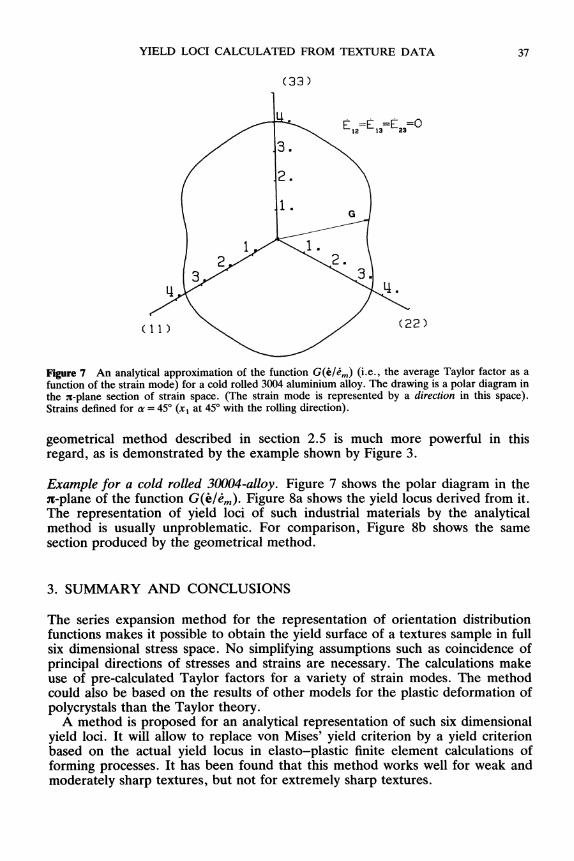
Figure 7 An analytical approximation of the function G(6/.m) (i.e., the average Taylor factor as afunction of the strain mode) for a cold rolled 3004 aluminium alloy. The drawing is a polar diagram inthe x-plane section of strain space. (The strain mode is represented by a direction in this space).Strains defined for a 45 (xl at 45 with the rolling direction).

geometrical method described in section 2.5 is much more powerful in thisregard, as is demonstrated by the example shown by Figure 3.

Example for a cold rolled 30004-alloy. Figure 7 shows the polar diagram in the-plane of the function G(/m). Figure 8a shows the yield locus derived from it.The representation of yield loci of such industrial materials by the analyticalmethod is usually unproblematic. For comparison, Figure 8b shows the samesection produced by the geometrical method.

3. SUMMARY AND CONCLUSIONS

The series expansion method for the representation of orientation distributionfunctions makes it possible to obtain the yield surface of a textures sample in fullsix dimensional stress space. No simplifying assumptions such as coincidence ofprincipal directions of stresses and strains are necessary. The calculations makeuse of pre-calculated Taylor factors for a variety of strain modes. The methodcould also be based on the results of other models for the plastic deformation ofpolycrystals than the Taylor theory.A method is proposed for an analytical representation of such six dimensional

yield loci. It will allow to replace von Mises’ yield criterion by a yield criterionbased on the actual yield locus in elasto-plastic finite element calculations offorming processes. It has been found that this method works well for weak andmoderately sharp textures, but not for extremely sharp textures.

38 P. VAN HOUTTE ET AL.

(a)

Stt/a"

,z=S,==S=3=O

S2z/T

(b)

Figure $ (a) -plane section of the yield locus of a cold rolled 3004 aluminium alloy (analyticalmethod). Stresses defined for re= 45 (xl at 45 with the rolling direction). (b) Idem, geometricalmethod.


ReferencesAernoudt, E., Gil-Sevillano, J. and Van Houtte, P. (1987). Constitutive Relations and Their Physical

Basis (Proc. 8th Ris5 International Symposium on Metallurgy and Materials Science), pp. 1-38, S. I.Andersen, J. B. Bilde-S6rensen, N. Hansen, T. Leffers, H. Lilholt, O. B. Pedersen and B. Ralph,eds., Ris6 National Laboratory, Roskilde, Denmark.

Berveiller, M. and Zaoui, A. (1984). J. Engng. Mater. Technol. 106, 295-298.Bunge, H. J. (1970). Kristall und Technik 5, 145-175.Bunge, H. J. (1982). Texture Analysis in Material Science, Butterworths, London.Bunge, H. J., Schulze, M. and Grzesik, D. (1980). Peine-Salzgitter Berichte, Sonderheft.Hill, R. (1950). The Mathematical Theory of Plasticity, Clarendon Press, Oxford.Lequeu, Ph., Gilormini, P., Montheillet, F., Bacroix, B. and Jonas, J. J. (1987). Acta Metall. 35,

439-451.Molinari, A., Canova, G. R. and Ahzi, S. (1987). Acta Metall. 35, 2983-2994.Mols, K., Van Praet, K. and Van Houtte, P. (1984). Proc. Seventh Intntl. Conf. on Textures of

Materials (ICOTOM 7), pp. 651-656, C. M. Brakman, P. Jongenburger and E. J. Mittemeijer,eds., Netherlands Society for Material Science, Zwijndrecht (The Netherlands).

Sowerby, R., Da Viana, C. S. and Davies, G. J. (1980). Mat. Sci. Eng. 46, 23-51.Van Houtte, P. (1987). Textures and Microstructures 7, 29-72.Van Houtte, P. (1988). Textures and Microstructures, 8-9, 313-350.

YIELD LOCI FROM TEXTURE DATA

Documents

Transcript of YIELD LOCI FROM TEXTURE DATA