(Yearsley, 2003)

United States EPA Region 10 910-R-03-003 Environmental Protection Agency (OEA-095) December 2003

Developing a Temperature Total Maximum Daily Load for the Columbia and Snake Rivers: Simulation Methods

John Yearsley EPA Region 10 Seattle, Washington

United States EPA Region 10 910-R-03-003 Environmental Protection Agency (OEA-095) December 2003

4

Developing a Temperature Total Maximum Daily Load

for the Columbia and Snakes Rivers: Simulation Methods

Introduction The States of Idaho, Oregon and Washington and the U. S. Environmental Protection Agency (EPA) are working in coordination with the Columbia Basin Tribes to develop Total Maximum Daily Loads (TMDL) for Temperature and Total Dissolved Gas (TDG) on the Columbia and Snake Rivers. A TMDL for a water body is a document that identifies the amount of a pollutant that the water body can receive and still meet Water Quality Standards (WQS). A TMDL also allocates responsibility for reductions in the pollutant load that are necessary to achieve WQS. A TMDL is required by the Clean Water Act for any stream reaches included by States or Tribes on their lists of impaired waters required under Section 303(d) of the Clean Water Act. Impaired waters are those that do not attain State or Tribal Water Quality Standards (WQS). The Snake River from its confluence with the Salmon River at RM 188 to its confluence with the Columbia River has been included on the 303(d) list of impaired waters for Temperature and TDG by Idaho, Oregon or Washington as appropriate. Oregon and Washington included all of the Columbia River on their 303(d) lists for TDG and most of the Columbia River on their lists for Temperature. The Columbia River also exceeds the WQS of the Colville Confederated Tribes for Temperature and TDG. The Spokane Tribe of Indians has WQS for the Columbia River that have been adopted by the Tribe but not yet approved by EPA. These standards are also exceeded in the Columbia River. The states of Idaho, Oregon and Washington have assumed responsibility for developing TMDL’s for total dissolved gas for their respective waters in cooperation with the dam operators within their boundaries. EPA is working with the Colville Tribe and the Spokane Tribes for the portion of the dissolved gas TMDL within reservation boundaries. Oregon DEQ and Washington DOE will collaborate on the total dissolved gas TMDL for the interstate portions of the Columbia River. The purpose of the Columbia and Snake River main stem temperature TMDL is to understand the sources of temperature loadings and to allocate those loadings to meet state and tribal water quality standards. EPA Region 10 is the technical lead for the temperature TMDL. EPA Region 10 has chosen the mathematical model, RBM10, developed by EPA Region 10 (Yearsley et al, 2001) as the technical basis for developing a TMDL for temperature for the Snake/Columbia Main stem.

Model Description RBM10 (Yearsley et al, 2001) is a dynamic, one-dimensional model that simulates water temperature using the energy budget method. It was originally developed to perform a

5

temperature assessment of the Snake River from Lewiston, Idaho to its confluence with the Columbia and of the Columbia River from Grand Coulee Dam to Bonneville Dam. The model implements a mixed Eulerian-Lagrangian method for solving the dynamic energy budget equation. The model uses reverse particle tracking to locate the starting point of a water parcel at each computational time step. The water temperature at the starting point of each time step for a parcel is determined by polynomial interpolation of simulated temperatures stored on a fixed grid. The energy budget method (Wunderlich and Gras, 1967) is used to simulate the time

history of temperature as the parcel moves from its starting point at time, t- t, to ending point at time, t. Kalman filtering is used to account for uncertainty in the water temperature data used to develop the model.

Conceptual Approach One-dimensional models have been used to assess water temperature in the Columbia River system for a number of important environmental analyses. The Federal Water Pollution Control Administration developed and applied a one-dimensional thermal energy budget model to the Columbia River as part of the Columbia River Thermal Effects Study (Yearsley, 1969). The Bonneville Power Administration and others used HEC-5Q, a one-dimensional water quality model, to provide the temperature assessment for the Columbia River System Operation Review (BPA, 1994). Normandeau Associates (1999) used a one-dimensional model to assess temperature conditions in the Lower Snake River for the US Army Corps of Engineers. Perkins and Richmond (2001) used the one-dimensional temperature model, MASS1, to simulate both the impounded and unimpounded Snake rivers. The water quality standards for most of the subject river reaches are written so as to limit the increase in water temperatures as a result of human activities (Washington WQS) or anthropogenic activities (Oregon WQS). This requires an estimate of temperature conditions in the absence of the human activities. The conceptual approach used in the development of the temperature TMDL is based on the notion that the effect of “human activities” can be estimated by simulating conditions in the unimpounded river segments with no point sources present. These results can then be used to determine the impacts of human activities associated with hydroelectric projects, water withdrawals and point source discharges. An important assumption in this approach is that impacts of “human activities” on water temperature outside the geographical limits of this analysis will be addressed by other TMDL’s or water quality plans; that water quality and quantity at the boundaries of this TMDL are the result of existing upstream activities.

Model Development Much of the model development was done in the problem assessment phase of the TMDL and is described in Yearsley et al (2001). Although the basic mathematical structure of the model was not changed, the model framework was changed in a number of ways to accommodate the needs of the TMDL.

6

Model Domain The Columbia River and the Snake River (Figure 1) are listed by the states of Oregon and Washington as water-quality limited under Section 303(d) of the Clean Water Act. Listed segments of these rivers in the model domain for the TMDL include the Columbia River from the International Boundary (Columbia River Mile 745.0) to the Pacific Ocean near Astoria, Oregon and the Snake River from its confluence with the Salmon River (Snake River Mile 188.2) to its confluence with the Columbia River near Pasco, Washington (Columbia River Mile 324.0). In addition, the Clearwater River from Orofino, Idaho (Clearwater River Mile 44.6) to its confluence with the Snake River near Lewiston, Idaho (Snake River Mile 139.3) was included in the model domain. The Clearwater River was included because of the influence releases from Dworshak Dam on the North Fork of the Clearwater have on water temperatures of the Snake River downstream from Lewiston. Although the Clearwater is not listed as water-quality limited under Section 303(d), it may have an important role in any implementation plans developed from the TMDL. Major tributaries to the Columbia River and Snake River (Table 1) are included in the model domain simply as point source inputs. That is the temperatures are not simulated, rather the advected energy is treated as data input. While some of these tributaries are listed as water-quality limited for temperature, any improvement in temperature that may result from TMDL’s written for these segments is not considered in this analysis. There are two reasons for this. The size of these tributaries is such that their impact on the well-mixed temperature of the Columbia is small. Furthermore, any temperature improvement in the development of TMDL’s on the tributaries will be included in the interpretation of the States’ water quality standards as described below. Data Requirements Data requirements for simulating water temperatures with RBM10 include the following

The speed of the parcel along its characteristic path and the geometric properties of the river are estimated from functional relationships between flow and geometry. A gradually varied, steady flow model (USACE-HEC 1995) is used to establish the functional relationships between flow and geometry. The basic data needed to establish these relationships are depth as a function of width at various cross-sections. For the purposes of the TMDL, data of this type were acquired from a number of sources as described in Yearsley et al (2001).

The energy budget is developed from meteorological data. The data are wind speed, dry bulb temperature, relative humidity (or similar measure of water content), cloud cover, and station pressure as a function of time.

Advected thermal energy is defined by the stream flow and water temperature of headwaters, tributaries and points sources.

7

Parameter Estimation The basic model framework for the TMDL was developed in the problem assessment and described in Yearsley et al (2001). In the problem assessment the parameter estimation process was implemented using a smaller model domain and water temperature data from the period 1990-1994. For the TMDL, the parameter estimates were updated using the larger model domain and water temperature data from the period 1995-1999. The water temperature data are from monitoring sites below the dams and appear to be of higher quality and more representative of well-mixed river temperatures. Station descriptions for the Columbia and Snake rivers are given in Tables 2 and 3,respectively. The only parameter estimated was the coefficient, Ke, in the relationship describing the rate of heat transfer due to evaporation

)e - L(eK q aweevap

where, qevap = the heat flux across the air-water interface due to evaporation,

= the density of water, L = the latent heat of vaporization, ew = the saturated vapor pressure at the water surface temperature, ea = the vapor pressure of the air above the water. The energy budget for the model domain of the TMDL analysis is characterized by five different meteorological provinces as described above (Table 4). The coefficient, Ke, was treated as a variable for each meteorological province. The parameter estimation process was designed to select the set of coefficients, Ke , that resulted in the minimum mean squared difference, between simulated and observed for the monitoring sites shown in Table 5. Model Acceptance Statistics used to assess performance of the one-dimensional mathematical model, RBM10, are similar to those described as appropriate for temperature models (Bartholow, 1989) and recommended by van der Heijde and Elnawawy (1992) in EPA’s guidance for selecting groundwater models. The performance measures calculated for the TMDL simulations include: Mean Difference

Dmean = N

)-T(T1

obssim

N

n

8

Absolute Mean Difference

Damd = N

|-TT|1

obssim

N

n

Root-Mean-Squared Difference

Drms = N

2)-T(T1

obssim

N

n

where, N = the number of matched pairs of simulated and observed temperatures, Tsim = the simulated temperature at the time of the nth observation Tobs = the observed temperature. The model performance statistics for the five-year (1995-1999) simulation period are given in Table 5.

TMDL Analysis Several types of simulations were used in the development of the temperature TMDL for the Columbia and Snake rivers. Table 6 gives a summary of the simulation types. Simulation results are reported at the compliance points as described in the TMDL . The compliance points are just downstream from hydroelectric projects or, in the case of the unimpounded portion of the Columbia River below Bonneville Dam, the compliance points are generally downstream from major discharges. All the data and model source codes for developing the TMDL are on the data CD (Appendix A). The following discussion describes the contents of the directories on the data CD. The computer programs and data files can be used to reproduce all the results used in the Final Draft Temperature TMDL for the Columbia and Snake rivers. Each of the headings below is the name of a directory on the data CD, Appendix A. File and directory names are given in boldface. \Appendix_A\Forcing_Functions

9

The files containing thirty-year record (1970 through 1999) of energy inputs to the system are stored in this directory. Thermal energy inputs to the river system are from advected sources (main stem boundaries and tributaries) and heat transfer across the air-water interface. Advected thermal energy from tributaries and main stem boundaries are estimated from river flow and water temperatures. Data for advected thermal energy were obtained from the sources shown in Tables 2 and 3. Missing water temperature data were filled by linear interpolation when data gaps were of the order of a week or less. For larger gaps, a lag-one Markov model was used to fill in missing data. Heat transfer across the air-water interface is estimated from the meteorological data. Meteorological data from six weather stations are used to estimate the energy budget for the TMDL. The weather stations used in the TMDL and the segments of river are defined in Table 4. Weather data for these stations are in the directory, \Appendix_A\Meteorology\.. Only three of the weather stations, Lewiston, Portland and Yakima, are primary stations, ones where all the required meteorological variables are measured and reported. The other three weather stations, Coulee Dam, Wenatchee and Richland, report only air temperature. The remaining meteorological data for these stations was synthesized from the the primary station as shown in Table 4. The energy budget files were created in the folder, ..\System_iv\setup, using the programs, build_heat.exe, and energy.exe. The source code for build_heat.exe, and energy.exe has hard-wired coding that looks for weather data in specific directories. The code should be modified to ensure that the pathways specified in the coding are correct for the particular application The output files with energy budget are named, CityName.budget.avg, as in, Portland.budget.avg. The file with thermal energy from advective sources (main stem boundary conditions and tributaries) is named, No_Ocean.advect. The file with elevation data is named, No_Ocean.elev. These files were created in the folder, ..\System_iv\setup using the program, start_iv.exe in conjunction with the control file. no_ocean.control. These advection and elevation files were used as the forcing functions for all the scenarios simulated for the TMDL. \Appendix_A\TMDL\Site_Potential The framework for implementing the State of Washington’s water quality standards is constructed around the concept of “site potential.” Site potential, in the case of the temperature TMDL, is defined as the daily-averaged, cross-sectional average temperature that would result in the absence of impoundments and discharges of thermal energy from municipal and industrial point sources as well as from various nonpoint sources. As described above, those impacts on the thermal energy budget external to the defined boundaries of the temperature TMDL are considered to be part of site potential. These impacts include those changes in flow and temperature at the boundaries of the TMDL resulting from human activities. Non-stationary impacts on climate such as global warming from industrial carbon dioxide production may also be present in site potential as defined and realized with the inputs described below. Site-potential is not, therefore, the temperature of the river prior to human development. Rather it is the temperature that would result in the absence of major human activities in the listed river segments.

10

Human activities in the existing river system configuration that have altered the thermal regime of the Columbia and Snake rivers are:

1. Construction of impoundments for hydroelectric facilities and navigational locks, which increase the time waters of the Columbia and Snake are exposed to high summer temperatures, increase the surface area exposed energy transfer across the air-water interface and change the system’s thermal response time.

2. Discharge of thermal energy from industrial and municipal point sources and agricultural and urban nonpoint sources

3. Hydrologic modifications to the natural river system to generate electricity, provide irrigation water for farmlands, and facilitate navigation.

4. Modifications of the watershed by urban development and agricultural and silvicultural practices that reduce riparian vegetation, increase sediment loads, and change stream or river geometry.

The TMDL focuses on those activities associated with the construction of impoundments, thermal discharges from point and nonpoint sources and, implicitly, on the effects of hydrologic modifications. The TMDL’s developed for the listed tributaries of the Columbia and Snake rivers should develop water quality plans that address thermal effects of modifications of the watershed.

The impacts of impoundments on the thermal regime of the Columbia and Snake rivers are due to both the change in river geometry and to operation of the hydroelectric facilities. All of the hydroelectric projects within the model domain, with the exception of Grand Coulee Dam, are run-of-the river projects. That is, the projects are operated such that approximately all the water entering the reservoir is passed through the reservoir and released. As a result, the water level in these reservoirs fluctuates very little. This does not mean the effects of the operation do not have ecological impacts. It is well known, for example, that daily fluctuations in tailwater elevations at Priest Rapids affect spawning and rearing habitat of fall Chinook and can cause stranding of juvenile fish in the Hanford Reach of the Columbia River (Tiffan, 2003). However, the impact of these operations on the daily-averaged, cross-sectional average temperature is small. The major impact on the daily-average, cross-section water temperature is due to the increase in width and depth resulting from the construction and operation of the impoundment.

Flood control is an operational feature of Lake Roosevelt, the reservoir behind Grand Coulee Dam. As a result, the fluctuations in reservoir elevation are significant (Figure xx). Therefore, simulations of water temperature for the existing conditions include the effects of storage for this project.

Point source inputs for the TMDL analysis are based on permit numbers provided by the State of Oregon’s Department of Environmental Quality (DEQ) and the State of Washington’s Department of Ecology (DOE). The energy inputs associated with these sources are given in Table 8. Major discharges are shown individually while smaller discharges are aggregated and shown as aggregated sources at the end of certain river reaches. In addition, a 20 megawatt

11

allowance of thermal energy is provided at each compliance point for general permits. general permit includes impacts from stormwater discharge

The model domain for simulating site potential was created with the hydraulic properties in the file crtes.model.input.no_dams in the directory. A 30-year period of site potential temperatures were simulated for the model domain using hydrologic data and weather data for the period 1970 through 1999 and output to the files, Columbia.no_dams.avg and Snake.no_dams.avg for the Columbia River and the Snake River, respectively. A 30-year period of daily cross-sectionally averaged temperatures for existing conditions were simulated for the model domain using hydrologic data and weather data for the period 1970 through 1999 using the executable rbm10_iii.exe. The control file used for simulating existing conditions is crtes.model.input.dams. The simulation results were output to the files, Columbia.dams.avg and Snake.dams.avg for the Columbia River and the Snake River, respectively.

\Appendix_A\TMDL\Point_Sources

The impact of point sources at compliance points was simulated by comparing the simulated results from existing conditions, described above, with those same conditions when permitted thermal sources are removed. Environmental forcing functions and parameters were the same as those used for simulations of site potential and existing conditions. The basic source code for RBM10 was modified to accommodate the addition of point sources. The source code is in ..\Model_iii_pnt\rbm10_iii and is named rbm10_pnt.f. The executable is named rbm10_iii_pnt.exe.

Simulations were performed in two directories, ..\Existing_Sources and ..\Zero_Discharge using rbm10_iii_pnt.exe (point source version) in conjuncton with the control file, crtes.model.input.dams. The Fortran source code, rbm10_iii_pnt.f, in the directory, ..\Existing_Sources, differs slightly from that in the directory, ..\Zero_Discharge. The difference is due to hardwired coding that ignores point sources in the directory, ..\Zero_Discharge. The source code for each version is stored in the appropriate directory. This version of the control file has also been modified to accommodate the point sources. Simulated results are output at the compliance points as, ..\Existing_Sources\Columbia_Exist.RM_xxx, ..\Zero_Discharge\Columbia_Zero.RM_xxx, ..\Existing_Sources\Snake_Exist.RM_xxx, ..\Zero_Discharge\Snake_Zero.RM_xxx, where “xxx” is the river mile of the compliance point. The directory labeled, Existing_Sources, incorporates the thermal loadings associated with the point sources, while the directory labeled, Zero_Discharge, simulated the impounded system with no thermal discharges from point sources.

\Appendix_A\TMDL\Dam_Impacts

12

The effect of adding individual hydroelectric projects to the unimpounded river was simulated by starting with the river systems in their present configuration of hydroelectric projects. Simulations of the system were then performed by changing, one hydroelectric project at a time, the hydraulic coefficients of the portion of the river upstream of the dam from freely-flowing river type to reservoir type. This assumes that the impounded section of the river associated with a specific hydroelectric project will not affect the hydraulic characteristics of the unimpounded river both upstream and downstream of the of the project being evaluated. Environmental forcing functions and parameters were the same as those used for other simulations. Results are in,..\DamName\, where “DamName” is the name of the hydroelectric project.

Simulations were performed with the same forcing functions used for other scenarios and the version of the source code used for the characterization of site potential. The version of the source code is labeled, rbm10_ iii.f, in the directory, ..\Model_III\rbm_iii\Original_Code. The executable associated with this source code, rbm10_iii.exe, was used in conjunction with control file for each each dam and labeled crtes.model.final.nnn, where, nnn, is the symbol for the specific dam as in the example, crtes.model.final.BON, the file containing simulated effect of adding Bonneville Dam to the unimpounded river.

\Appendix_A\TMDL\Obverse_Impacts

For purposes of the TMDL, the impact of individual dams was simulated by changing, one project at a time, the hydraulic properties of the reservoir behind the dam to hydraulic properties representing the freely-flowing river. As in the case above where individual dams were added to the natural river system, this set of scenarios assumes that the hydraulic properties of the freely-flowing river will not be affected significantly by hydroelectric projects upstream or downstream from the one being evaluated. Environmental forcing functions and parameters were the same as those used for other simulations. Results are in,..\DamName\, where “DamName” is the name of the hydroelectric project.

Simulations were performed with the same forcing functions used for other scenarios and the version of the source code used for the characterization of site potential. The version of the source code is labeled, rbm10_ iii.f, in the directory, ..\Model_III\rbm_iii\Original_Code. The executable associated with this source code, rbm10_iii.exe, was used in conjunction with control file for each each dam and labeled DamName.Obverse, where, DamName, is the symbol for the specific dam as in the example, Bonneville, for Bonneville Dam.

Output for the simulations in the Columbia and Snake rivers is to files named RiverName.nnn.Obv. RiverName is either Columbia or Snake and nnn, is the symbol for the specific dam as in the example, Columbia.BON.Obv, for the file with the simulated effects of removing Bonneville Dam from the impounded river.

13

\Appendix_A\TMDL\Work_Space

The software that implements RBM10, the time-dependent, one-dimensional energy budget model, was modified such that simulated results could be compared to the water quality standards of Washington and Oregon. The reference data sets used for making comparisons were the simulations based on site potential (COLUMBIA.NO_DAMS.AVG and SNAKE.NO_DAMS.AVG). The modified program is named RBM10_TMDL.F and is located in the directory \Appendix_A\TMDL\Work_Space\RBM_TMDL.

Several TMDL scenarios were evaluated using the RBM10 model framework. 21 of these scenarios, including the scenario used for the draft final TMDL are in the directory, \Appendix_A\TMDL\Work_Space\TMDL_final. All but the scenario used for the draft final TMDL, Scenario_21a, are archived in the compressed file, Scenario_Archive.zip. A brief description of the 21 scenarios is in the document, \Appendix_A\TMDL\Work_Space\Work_Space_log.doc.

The first step in the TMDL was to allocate loads to the permitted discharges. The simulations of point sources described above provided estimates showing that the far-field temperature effects of permitted discharges did not exceed the water quality standards of the states of Oregon and Washington. The point sources were, therefore, allocated thermal loads based on their National Pollution Discharge Elimination System (NPDES) permits. The allocations for the dams were determined from the results of the obverse impacts analysis. That is, each dam was allocated a temperature change based on the daily-averaged difference between simulated results for the existing system and the results when the particular dam was removed from the system. The file containing the allocations is named “DELTA.TMDL”. The results were compared with the water quality standards of the states or Oregon and Washington to assure compliance.

\Appendix_A\TMDL\Hourly_Max

Hourly water temperatures in the Columbia and Snake rivers were simulated using hourly meteorological data and daily averaged temperature and flow data. Hourly simulations were performed for calendar years 1992 and 1997 and the results saved in the directory, \Appendix_A\TMDL\Hourly_Max\Results. The forcing functions for advection and energy transfer across the air-water interface are the advection file, No_Ocean.advect, and meteorological data files CityName.199x.hourly, where “CityName” is the name of the weather station “x” is either “2” or “7”, as in the example, Lewiston.1992.hourly.

The source code, rbm10_iii.f, is the same as that used to develop the site potential.

14

Figure 1. Model domain for Columbia and Snake rivers water temperature TMDL

16

References

Bartholow, J.M. 1989. Stream temperature investigations—Field and analytic methods. Instream Flow and Info. Paper No.13. U.S. Fish and Wildlife Service.

Bonneville Power Administration et al. 1994. Columbia River system operation review. Appendix M, Water quality. DOE/EIS-0170. Bonneville Power Administration, U.S. Army Corps of Engineers, and U.S. Bureau of Reclamation, Portland, Oregon.

Normandeau Associates. 1999. Lower Snake River temperature and biological productivity modeling. R-16031.007. Preliminary review draft. Prepared for the Department of the Army, Corps of Engineers, Walla Walla, Washington.

Perkins, W.A. and M.C. Richmond. 2001. Long-term, one-dimensional simulation of Lower Snake River temperatures for current and unimpounded conditions. Battelle Pacific Northwest Laboratory, Richland, Washington. 86 pp.

Tiffan, K. 2003. Evaluation of the effect of water management on Fall Chinook spawning and rearing habitat and on stranding of juvenile Fall Chinook in the Hanford Reach of the Columbia River. http://wfrc.usgs.gov/research/fish%20populations/STRondorf8.htm viewed on

10/16/2003.

USACE-HEC (U.S. Army Corps of Engineers). 1995. HEC-RAS: River analysis system. U.S. Army Corps of Engineers, Hydrologic Engineering Center, Davis, California.

Van de Heijde, P.K.M. and O.A. Elnawawy. 1992. Quality assurance and quality control in the development and application of ground-water models. EPA/600/R-93/011. US Environmental Protection Agency, Office of Research and Development, Ada, Oklahoma. 68 pp.

Wunderlich, W.O., and R. Gras. 1967. Heat and mass transfer between a water surface and the atmosphere. Tennessee Valley Authority, Division of Water Cont. Planning, Norris, Tennessee

Yearsley, J.R. 1969. A mathematical model for predicting temperatures in rivers and river-run reservoirs. Working Paper No. 65, Federal Water Pollution Control Agency, Portland, Oregon.

Yearsley, J., D. Karna, S. Peene and B. Watson. 2001. Application of a 1-D heat budget model to the Columbia River system. Final report 901-R-01-001 by the U.S. Environmental Protection Agency, Region 10, Seattle, Washington

http://wfrc.usgs.gov/research/fish%20populations/STRondorf8.htm

18

Table 1. Tributaries of the Columbia and Snake rivers and sources of data for tributary flows and water temperatures

Data Sources

Flow Temperature

Salmon River at White Bird, Idaho

USGS 13317000 USGS 13317000

Grande Ronde River at Troy, Oregon

USGS 13333000 Washington DOE 35C070

Snake River near Anatone, Washington

USGS 13334300 USGS 13334300; DART Site

ANQW

Clearwater River at Orofino, Idaho

USGS 13340000 USGS 13340000

North Fork Clearwater at Dworshak Dam

DART Site DWR DART Site DWR

Tucannon near Starbuck, Washington

USGS 13344500 Washington DOE 35B060

Palouse River near Hooper, Washington

USGS 13351000 Washington DOE 34A070

Columbia River at the International Boundary

USGS 12399500 DART Site CIBW

Kettle River near Laurier, Washington


Colville River at Kettle Falls, Washington


Spokane River at Long Lake USGS 12433000 USGS 12433000

Feeder Canal at Grand Coulee, Washington

USGS 12435500 -----

Okanogan River at Malott, Washington


Methow River near Pateros, Washington


Wenatchee River at Monitor, Washington


Crab Creek near Moses Lake, Washington


Yakima River at Kiona, Washington


Walla Walla River at Touchet, Washington

USGS 14018500 USGS 14018500

Umatilla River near Umatilla, Oregon

USGS 14033500 USGS 14033500

John Day River at McDonald Ferry, Oregon

USGS 14048000 Oregon DEQ 404065

19

Table 1 (continued). Data sources for advected energy on the main stem Columbia and Snake Rivers

Deschutes River at Moody, near Biggs, Oregon


Klickitat River USGS 14105700 USGS 14113000

Hood River USGS 14120000 Oregon DEQ 402081

Sandy below Bull Run Reservoir, Oregon


Willamette River at Portland, Oregon

USGS 14211720 Constrained to Columbia River

Lewis River at Ariel, Washington USGS 14220500 Oregon DEQ 402081

Cowlitz River at Castle Rock, Oregon

USGS 14243000 Oregon DEQ402081

20

Table 2. Temperature monitoring sites in the Columbia River used to evaluate RBM10 model acceptance

Station

Station

Identifier

Station Description

Bonneville Dam tailwater BON Columbia RM 146: Right end of spillway near center of dam

The Dalles Dam tailwater TDDO Columbia RM 190: Left bank one mile d/s of dam

John Day Dam tailwater JHAW Columbia RM 215: Dam tailwater Right bank of river

McNary Dam tailwater-Washington MCPW Columbia RM 291: Dam Tailwater Right bank of river

Priest Rapids tailwater PRXW Columbia RM 396: Tailwater D/s of dam

Wanapum Dam tailwater WANW Columbia RM 415: Tailwater D/s of dam

Rock Island Dam tailwater RIGW Columbia RM 452: Tailwater D/s of dam

Rocky Reach Dam tailwater RRDW Columbia RM 472 Tailwater D/s of dam

Wells Dam tailwater WELW Columbia RM 514: Tailwater D/s of dam

Chief Joseph Dam tailwater CHQW Columbia RM 545: Tailwater D/s of dam

Grand Coulee Dam tailwater GCGW Columbia RM 590: Six miles D/s of dam

Table 3. Temperature monitoring sites in the Snake River used to evaluate RBM10 model acceptance

Station

Station

Identifier

Station Description

Ice Harbor Dam tailwater IDSW Snake RM 6.8: Right bank 15,400 feet d/s of dam

Lower Monumental Dam tailwater LMNW Snake RM 40.8:Left bank 4,300 feet d/s of dam

Little Goose Dam tailwater LGSW Snake RM 69.5:Right bank 3,900 feet d/s of dam

Lower Granite Dan tailwater LGNW Snake RM 106.8: Right bank 3,500 feet d/s of dam

21

Table 4. Meteorological stations used to estimate heat budget parameters for the Columbia and Snake rivers

Station Name Station # Station Type Station Used to

Synthesize River Segments

Lewiston, Idaho WBAN 24149 Surface Airways --- Snake RM 0.0 – 188.0

Clearwater RM 0 – 42.0

Portland, Oregon

WBAN 24229 Surface Airways --- Columbia RM 0.0 – 1245.5

Spokane, Washington

WBAN 24157 Surface Airways --- ---

Yakima, Washington

WBAN 24243 Surface Airways --- Columbia RM 292.0 – 453.4

Coulee Dam NCDC 451767 Local

Climatological Data

Spokane Columbia RM 738.0 – 596.5

Richland NCDC 457015 Local

Climatological Data

Yakima Columbia RM 292.0 – 145.5

Wenatchee NCDC 459074 Local

Climatological Data

Spokane Columbia RM 596.5 – 453.4

22

Table 5. Model performance statistics for RBM10. Statistics computed for the

difference between simulated and observed (Simulated-Observed)

Columbia River # of

Samples

Absolute Mean

Difference

Average Difference

RMS Difference

Standard Deviation

Grand Coulee 1150 0.73 -0.08 0.97 0.94

Chief Joseph 678 1.05 0.81 1.46 1.46

Wells 348 0.52 0.40 0.70 0.32

Rocky Reach 512 0.67 0.57 0.86 0.42

Rock Island 534 0.64 0.53 0.85 0.43

Wanapum 889 0.81 0.05 1.25 1.56

Priest Rapids 773 0.78 -0.09 1.03 1.06

McNary 1222 0.56 -0.34 0.72 0.40

John Day 666 0.46 0.02 0.59 0.35

The Dalles 703 0.43 0.06 0.54 0.29

Bonneville 493 1.07 -0.59 1.36 1.49

Snake River

Lower Granite 1144 0.83 -0.64 1.03 0.65

Little Goose 746 0.77 -0.29 1.13 1.19

Lower Monumental

819 0.73 -0.19 0.93 0.82

Ice Harbor 1222 0.78 -0.30 0.93 0.78

23

Table 6. Model Applications Used in Development of TMDL

RBM10 Application

Model Setup Output Files Findings

1. Site Potential Temperature

Daily Time Step Un-impounded River Existing tributary/boundary inflows No point sources

Columbia.no_dams.avg

Snake.no_dams.avg

Temperatures exceed numeric criteria (e.g., 20 deg C in lower Columbia) in absence of human activity on mainstems

2. Actual Temperature

Daily Time Step Impounded River Existing tributary/boundary inflows All point sources

Columbia.dams.avg

Snake.dams.avg

Actual temperatures are higher than site potential temperatures in late summer/fall (e.g., 3.5 deg C warmer at John Day dam)

3. Point Source Cumulative Impacts

Daily Time Step Impounded River Existing tributary/boundary inflows Point Sources - 2 scenarios Scenario 1: No point sources Scenario 2: All point sources

..\Zero_Discharge\

Columbia_Zero.RM_xxx

Snake_Zero.RM_xxx

..\Existing_Sources\

Columbia_Exist.RM_xxx

Snake_Exist.RM_xxx

Maximum, cumulative point source impact less than 0.14 deg C.

24

4. Individual Dam Impacts

Daily Time Step Impounded River Existing tributary/boundary inflows All point sources Dams - 16 scenarios - Scenario 1: all dams included Scenarios 2-16: one dam removed and effects evaluated

..\Obverse_Impacts

Columbia.nnn.Obv

Snake.nn.Obv

Maximum temperature increases due to dams range from 0.1 deg C (Rock Island) to 6.2 deg C (Grand Coulee)

25

Table 6 (continued). Model Applications Used in Development of TMDL

RBM10 Application

Model Setup Outputs Findings

5. TMDL Target Temperatures

Daily Time Step Un-impounded River Existing tributary/boundary inflows All point sources Dams - 2 seasons: Aug-Oct Mean daily effect from 5 dams (Wells, Rocky Reach, Rock Island, Priest Rapids, and The Dalles), zero effect from remaining dams Nov-Feb Mean daily effect from 5 dams (Wells, Rocky Reach, Rock Island, Priest Rapids, and The Dalles), 0.12 deg C effect from remaining dams

..\TMDL_Final\Scenario_21a\

Columbia_TMDL.RM_xxx

Snake_TMDL.RM_xxx

This model setup represents a fully allocated temperature increment, based on compliance with standards at RM42

26

6. Diurnal Fluctuation

Hourly time step Impounded and Un-impounded Existing tributary/boundary inflows

..\Hourly_max\Results

Columbia.no_dams.yyyy.hourly

Columbia.dams.yyyy.hourly

Snake.no_dams.yyyy.hourly

Snake.dams.yyyy.hourly

Greater diurnal fluctuations in un-impounded river than impounded river

29

Table 7. Point sources of thermal energy in the Columbia River

Facility

River Mile

Thermal Load (MW)

Allocation Flow, Q

(cfs) Temperature

(deg C)

Avista – Kettle Falls 702.4 1.374 Bubble 0.360 32.2 Grand Coulee - Chief Joseph 0.360 32.2

Grand Coulee Dam 596.6 0.906 Bubble 0.279 27.5

Grand Coulee 596.6 2.518 Bubble 1.063 20.0

City of Coulee Dam 596.0 1.099 Bubble 0.464 20.0

Chief Joseph - Wells Total 1.806 21.2

Chief Joseph Dam 545.1 0.030 Bubble 0.009 27.5

Bridgeport STP 543.7 1.510 Bubble 0.464 22.0

Brewster 529.8 1.832 Bubble 0.563 23.0

Patteros STP 524.1 0.414 Bubble 0.127 23.0

Wells - Rocky Reach Total 1.164 22.6

Wells Dam 515.8 0.004 Bubble 0.002 20.0

Wells Hydro Project 515.0 0.015 Bubble 0.006 20.0

Chelan STP 503.5 7.399 Bubble 2.274 25.0

Entiat STP 485.0 0.604 Bubble 0.186 23.0

Rocky Reach - Rock Island Total 2.468 24.8

Rocky Reach Dam 474.9 0.020 Bubble 0.006 27.5

Tree Top 470.8 0.331 Bubble 0.127 22.0

Naumes Processing 470.5 10.543 Bubble 2.674 33.3

Columbia Cold Storage 466.3 5.990 Bubble 0.928 23.9

E Wenatchee STP 465.7 19.126 Bubble 5.879 23.5

KB Alloys 458.5 1.484 Bubble 0.464 27.0

Specialty Chemical 456.3 15.464 Bubble 6.189 21.1

Alcoa Wenatchee 455.2 17.847 Bubble 6.962 21.6

Rock Island - Wanapum Total 23.230 23.5

Rock Island 453.4 0.008 Bubble 0.002 27.5 Rock Island West Powerhouse 453.4 0.008 Bubble 0.002 27.5

Vantage STP 420.6 0.438 Bubble 0.135 26.0

Wanapum - Priest Rapids Total 0.139 26.0

Priest Rapids - McNary

Columbia Generating Sta 351.8 53.697 Bubble 15.114 30.0

Fluor Daniel Hanford, Inc 347.0 27.902 Bubble 8.475 27.8

Richland STP 337.1 57.378 Bubble 17.638 23.5

Baker Produce 329.2 0.040 Bubble 0.012 27.5

Twin City Foods 328.3 0.041 Bubble 0.012 28.3

Kennewick 328.0 61.405 Bubble 18.876 23.0

Pasco 327.6 22.752 Bubble 6.993 27.5

Total 67.121 25.8

31

Table 7(continued). Point sources of thermal energy in the Columbia River

Facility

River Mile

Thermal Load (MW)

Allocation Flow, Q

(cfs) Temperature

(deg C)

Agrium Bowles Road 322.6 405.821

Individual 62.150 28.1

62.150 28.1

Agrium Game Farm Road 321.0 484.694


102.410 31.7

Sanvik Metals 321.0 0.920 Individual 0.388 20.0

0.388 20.0

Boise Cascade Walulla 316.0 234.905


McNary to John Day 51.200 47.0

Umatilla STP 289.0 Individual 0.780 23.0

Goldendale 216.7 39.813 Individual 12.888 26.1

John Day - The Dalles 12.888 26.1

Biggs OR 208.8 0.236 Bubble 0.084 23.9

Wishram STP 200.8 0.488 Bubble 0.234 25.2

The Dalles - Bonneville Total 0.234 25.2

Dalles/Oregon Cherry OR 189.5 7.877 Bubble 2.784 23.9

Northwest Aluminum OR 188.9 8.793 Bubble 2.228 33.3

Cascade Fruit OR 188.3 0.875 Bubble 0.309 23.9

Lyle 183.2 0.008 Bubble 0.930 28.0

Mosier OR 174.6 0.131 Bubble 0.046 23.9

Total 6.298 27.8

SDS Lumber 170.2 160.323


16.240 28.3

Bingen STP 170.2 4.027 Bubble 1.238 23.0

Hood River OR 168.4 0.438 Bubble 0.155 23.9

Cascade Locks OR 151.0 0.381 Bubble 0.135 23.9

Stevenson STP 150.0 1.830 Bubble 0.696 22.2

Bonneville - Coast Total 2.223 22.9

Tanner OR 144.2 1.113 Bubble 0.392 24.0

North Bonneville STP 144.0 0.508 Bubble 0.193 22.2

Multnomah Falls OR 134.2 0.186 Bubble 0.059 26.7 BBA Nonwovens Washougal 124.0 0.336 Bubble 0.155 18.3

Exterior Wood, Inc. 123.8 0.295 Bubble 0.077 32.2

Washougal STP 123.5 9.111 Bubble 3.466 22.2

Camas STP 121.2 24.812 Bubble 9.438 22.2

Total 13.780 22.3

Georgia Pacific 120.0 313.206


33

Table 7 (continued). Point sources of thermal energy in the Columbia River

Facility

River Mile

Thermal Load (MW)

Allocation Flow, Q

(cfs) Temperature

(deg C)

Toyo Tanso USA OR 118.1 0.196 Bubble 0.071 23.4

Gresham OR 117.4 106.708 Bubble 39.176 23.0

Marine Park 109.5 64.431 Bubble 24.755 22.0

Vancouver Ice & Fuel Oil 106.0 0.005 Bubble 0.002 20.0

Graphic Packaging OR 105.6 31.503 Bubble 9.852 27.0

Northwest Packing Co. 105.2 0.348 Bubble 0.077 30.0

Portland STP OR 105.0 521.939 Bubble 195.881 22.5

Great Western Malting 105.0 36.278 Bubble 15.317 20.0

Vancouver Westside STP 105.0 183.024 Bubble 71.093 21.7

Support Terminal Services 104.8 0.008 Bubble 0.002 16.0

Clark County PUD 103.2 5.198 Bubble 1.099 40.0

Van Alco 103.0 25.321 Bubble 7.705 27.8

Salmon Creek STP 95.5 38.236 Bubble 14.544 22.2

Total 379.574 22.5

Boise/St Helens OR 85.8 219.555


Columbia River Carbonates 83.5 5.898 Individual 1.547 32.2

Coastal St Helens OR 82.6 365.094 Individual 77.266 39.9

Clariant Corp 76.0 5.894 Bubble 1.547 32.2

Kalama STP 75.0 1.627 Bubble 0.619 22.2

Noveon Kalama, Inc 74.0 7.450 Bubble 1.547 40.7

Steelscape, Inc. 73.5 1.885 Bubble 0.278 57.2

Total 3.992 35.7

PGE Trojan OR 72.7 511.152


Port of Kalama 72.2 0.081 Bubble 0.031 22.2

Riverwood OR 70.2 0.072 Bubble 0.025 24.0

Cowlitz STP 68.0 109.027 Bubble 41.766 22.0

Longview Fiber 67.4 540.993 Bubble 116.530 33.0

Rainier OR 67.1 2.436 Bubble 0.979 21.0

Cytec Industries 67.0 3.232 Bubble 1.516 22.0

Houghton International 67.0 0.008 Bubble 0.016 27.0

Total 160.864 30.0

Longview STP 66.0 10.983


Weyerhauser Longview 64.0 398.626 73.610 38.9

34

Individual

73.610 38.9

Reynolds 63.0 58.208 Bubble 24.600 20.0

Stella STP 56.4 0.014 Bubble 0.005 22.2

PGE Beaver OR 53.4 7.026 Bubble 1.695 35.0

New Source OR 52.8 24.841 Bubble 6.992 30.0

Total 33.293 20.0

GP Wauna OR 42.3 301.706


76.277 33.4

Cathlamet STP 32.0 0.549 Bubble 0.209 22.2

Astoria OR 11.8 23.383 Bubble 8.227 24.0

Ft. Columbia State Park 7.2 0.020 Bubble 0.008 22.2

Bell Buoy Crab Co. 6.0 0.329 Bubble 0.139 20.0

Warrenton OR 5.0 2.505 Bubble 0.881 24.0

Ilwaco STP 2.0 3.523 Bubble 1.083 20.0

Jessies Ilwaco Fish Co. 2.0 2.748 Bubble 1.160 16.0

Coast Guard Sta. 1.0 0.010 Bubble 0.003 27.5

Total 11.711 22.8

35

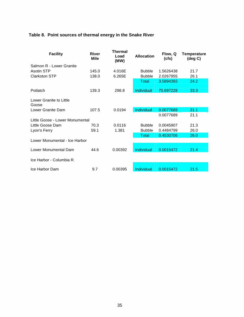
Table 8. Point sources of thermal energy in the Snake River

Facility

River Mile

Thermal Load (MW)

Allocation Flow, Q

(cfs) Temperature

(deg C)

Salmon R - Lower Granite

Asotin STP 145.0 4.016E Bubble 1.5626438 21.7

Clarkston STP 138.0 6.265E Bubble 2.0267955 26.1

Total 3.5894393 24.2

Potlatch 139.3 298.8 Individual 75.697228 33.3

Lower Granite to Little Goose

Lower Granite Dam 107.5 0.0194 Individual 0.0077689 21.1

0.0077689 21.1

Little Goose - Lower Monumental

Little Goose Dam 70.3 0.0116 Bubble 0.0045907 21.3

Lyon's Ferry 59.1 1.381 Bubble 0.4484799 26.0

Total 0.4530706 26.0

Lower Monumental - Ice Harbor

Lower Monumental Dam 44.6 0.00392 Individual 0.0015472 21.4

Ice Harbor - Columbia R.

Ice Harbor Dam 9.7 0.00395 Individual 0.0015472 21.5

(Yearsley, 2003)

Documents

Transcript of (Yearsley, 2003)