Yang-Baxter Solution of Dimers

as a Free-Fermion Six-Vertex Model

MATRIX, 7 July 2017

Paul A. Pearce & Alessandra Vittorini-Orgeas

School of Mathematics and Statistics

University of Melbourne

• PAP, A. Vittorini-Orgeas, arXiv:1612.09477.

0-1

Some History: Dimers & Dense Polymers

1961 Kasteleyn: Pfaffian solution of the dimer problem on the square lattice

1961 Temperley, Fisher: Independent solution on the square lattice

1967 Lieb: A non-Yang-Baxter transfer matrix method

2003 Izmailian, Oganesyan, Hu: Exact finite-size corrections of the free energy

for the square lattice dimer model under different boundary conditions

2005 Izmailian, Priezzhev, Ruelle, Hu: Logarithmic conformal field theory

and boundary effects in the dimer model

2007 Izmailian, Priezzhev, Ruelle: Non-local finite-size effects in the dimer model

2012 Rasmussen, Ruelle: Refined analysis of conformal spectra in the dimer model

2015 Nigro: Finite size corrections for dimers

2015 Morin-Duchesne, Rasmussen, Ruelle: Dimer representations of the

Temperley-Lieb algebra

2016 Morin-Duchesne, Rasmussen, Ruelle: Integrability and conformal data

of the dimer model

2007 Pearce, Rasmussen: Solution of critical dense polymers on the strip

2010 Pearce, Rasmussen, Villani: Solution of critical dense polymers on the cylinder

2013 Morin-Duchesne, Pearce, Rasmussen: Solution of critical dense polymers on the torus

0-2

Controversy/Approach

The Big Question:

• Is the dimer model a c = 1 Gaussian free theory or is it a c = −2 logarithmic CFT?

Strategy:

• Enumerate degrees of freedom (map to λ = π/2 six-vertex model).

• Introduce a spectral parameter (spatial anisotropy).

• Establish Yang-Baxter integrability (rotate faces by 45 degrees).

• Gain control to construct (r, s) type integrable/conformal boundary conditions on the strip.

0-3

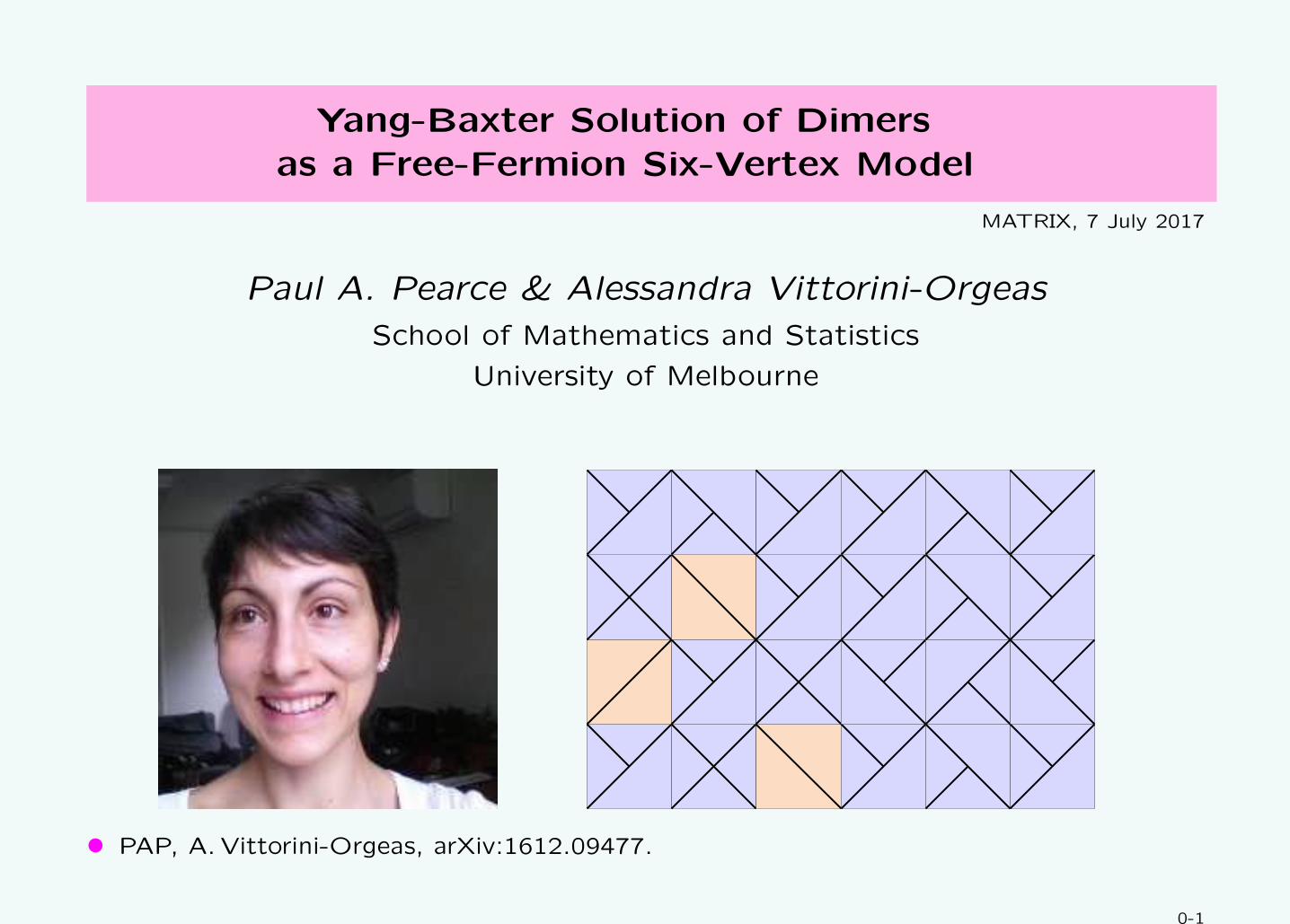
Usual Periodic Tiling of Horizontal and Vertical Dimers

• The known Pfaffian solution (Kasteleyn/Temperley-Fisher 1961) for the number of

periodic dimer configurations is

ZM×N = 12(Z

1/2,1/2M×N + Z

0,1/2M×N + Z

1/2,0M×N)

Zα,βM×N =

N/2−1∏

n=0

M/2−1∏

m=0

4

(

sin22π(n+ α)

N+ sin2

2π(m+ β)

M

)

, M,N = 2,4,6, . . .

• Explicit counting on a M ×N square lattice yields

(ZM×N) =

8 36 200 1156 · · ·36 272 3,108 39,952 · · ·200 3,108 90,176 3,113,860 · · ·1,156 39,952 3,113,860 311,853,312 · · ·

... ... ... ... . . .

N,M = 2,4,6, · · ·

⇓Z8×8 = 311,853,312

8 dimer configurations for a

2×2 lattice

0-4

Six-Vertex, Particle and Dimer Representations

• Equivalent tiles: Vertex, particle and dimer (Korepin&Zinn-Justin 2000) representations:

or

︸ ︷︷ ︸

a(u)︸ ︷︷ ︸

b(u)︸ ︷︷ ︸

c1(u)︸ ︷︷ ︸

c2(u)

At free-fermion point: λ = π2

a(u) = ρsin(λ− u)

sinλ= ρ cosu

b(u) = ρsinu

sinλ= ρ sinu

c1(u) = ρ g, c2(u) =ρ

g, ρ ∈ R

Counting isotropic dimers:

ρ = g =√2, u = λ

2 = π4

c1(u) = 2, a(u) = b(u) = c2(u) = 1

• The free fermion condition is satisfied at the free-fermion point λ = π2

a(u)2 + b(u)2 = c1(u)c2(u)

• Particle lines are drawn if arrows point down or left.

• Tiles corresponding to a source of horizontal arrows (apricot) have a double degeneracy.

Locally, the mapping is one-to-two for these faces. Sources and sinks of horizontal arrows

appear in pairs so g is a gauge which we fix to g = eiu.

0-5

Lattice Configurations

• A typical periodic configuration on a 6× 4 rectangular lattice: vertex, particle and (one of

the 23 = 8) possible dimer configurations:

• The boundary conditions are periodic so the left/right and top/bottom edges are identified.

• The excess of up arrows over down arrows along a row is conserved.

• Particles are conserved and move up and to the right around the torus but do not cross.

• The Z2 up-down arrow symmetry translates into a particle/hole duality.

• The particle trajectories are non-local (logarithmic) degrees of freedom.

• An M ×N rectangular lattice is covered by MN dimers. Each dimer covers two bonds of

the original square lattice.

0-6

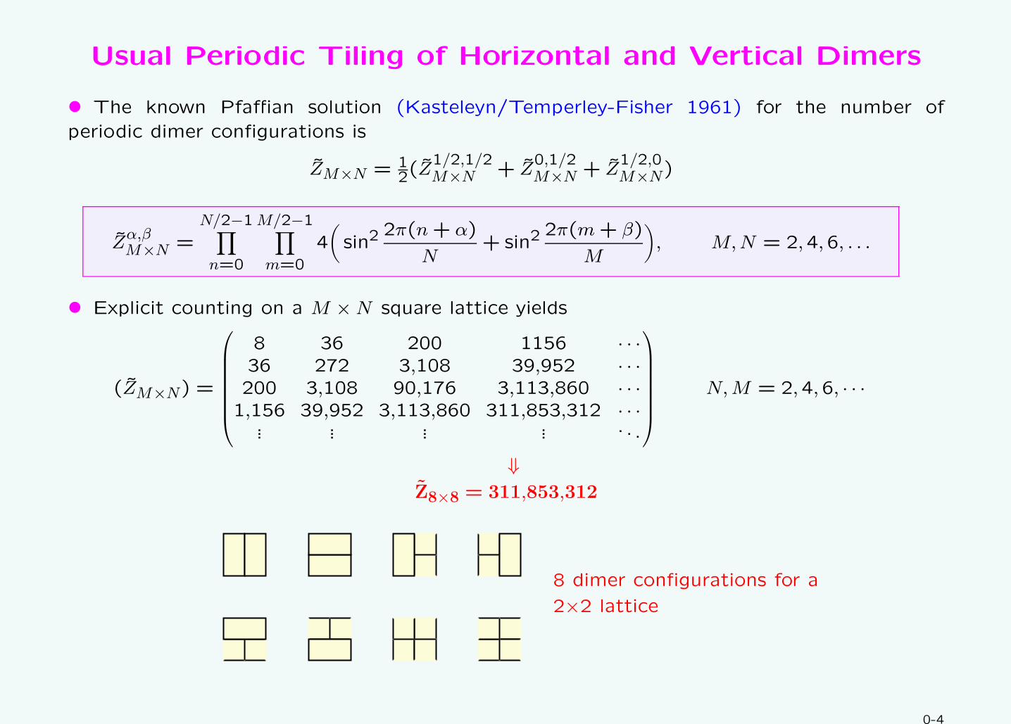
Fermionic Algebra

• In the particle representation, the face operators of the free-fermion six-vertex model

decompose into a sum of contributions from six elementary tiles

Xj(u) = uj j+1

= a(u)

(

+

)

+ b(u)

(

+

)

+ c1(u) + c2(u)

• As operators, the elementary tiles Ej act diagrammatically on an upper row particle

configuration to produce a lower row particle configuration

Ej = n00j , n11

j , f†j fj+1, f

†j+1fj, n10

j , n01j

• The (diagonal) number operators n1j and n0

j are orthogonal projectors that count the single

site occupancy and vacancies respectively at position j

nabj = na

jnbj+1, na

jnbj = δab n

aj , n0

j + n1j = I, n00

j + n11j + n10

j + n01j = I, a, b = 0,1

• In the hopping terms, fj and f†j are (non-diagonal) single-site particle annihilation and

creation operators respectively satisfying the CARs

{fj, fk} = {f†j , f†k} = 0, {fj, f†k} = δjk, n1

j = f†j fj, n0

j = fjf†j = 1− f

†j fj

0-7

More Fermionic Algebra

• The tiles are expressed as combinations of bilinears in fermi operators

= (1− f†j fj)(1− f

†j+1fj+1) = (1− f

†j fj)f

†j+1fj+1 = f

†j fj+1

= f†j fj f

†j+1fj+1 = f

†j fj(1− f

†j+1fj+1) = f

†j+1fj

• Multiplication of tiles in the fermionic algebra is given diagrammatically:

= = = =

= = = =

0-8

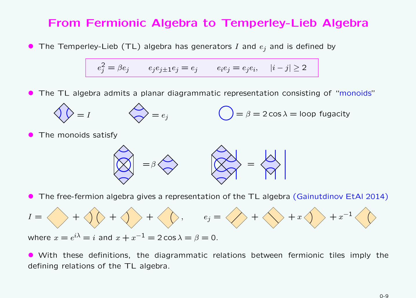
From Fermionic Algebra to Temperley-Lieb Algebra

• The Temperley-Lieb (TL) algebra has generators I and ej and is defined by

e2j = βej ejej±1ej = ej eiej = ejei, |i− j| ≥ 2

• The TL algebra admits a planar diagrammatic representation consisting of “monoids”

= I = ej = β = 2cosλ = loop fugacity

• The monoids satisfy

=β =

• The free-fermion algebra gives a representation of the TL algebra (Gainutdinov EtAl 2014)

I = + + + , ej = + + x + x−1

where x = eiλ = i and x+ x−1 = 2cosλ = β = 0.

• With these definitions, the diagrammatic relations between fermionic tiles imply the

defining relations of the TL algebra.

0-9

YBE and Inversion Relation

• In terms of the generators of the TL algebra, the face transfer operators of the free-fermion

six vertex/dimer model take the form

Xj(u) = u

j j+1

= cosu I + sinu ej

• This form of the face transfer operator is sufficient (Baxter 1982) to guarantee that Xj(u)

satisfies the Yang-Baxter Equation and Inversion Relation

Xj(v − u)Xj+1(v)Xj(u) = Xj+1(u)Xj(v)Xj+1(v − u), Xj(u)Xj(−u) = ρ2 cos2 u I

a b

v−u

ef

u

c

d

v =

de

v−u

b c

ua

f

v

cd

−u

a b

u

= ρ2 cos2 u δ(a, d)δ(b, c)

subject to the initial condition Xj(0) = I.

0-10

Commuting Periodic Row Transfer Matrices

YBE + Inversion ⇒ [T (u),T (v)] = 0 ⇒ Yang-Baxter Integrable

T (u)T (v) =

u u u u u

v v v v v• • • • • v − u• • •u− v

= • •v − uv v v v v

u u u u u• • • • • •• •u− v

=

v v v v v

u u u u u• • • • • •• •• •u− v • •v − u

= T (v)T (u)

• Since T (u)T = T (λ − u), the commuting row transfer matrices are normal and admit a

common set of eigenvectors independent of u. So they are simultaneously diagonalizable by

a similarity transformation.

• The eigenvalue spectra can be found by solving functional equations satisfied by T (u).

0-11

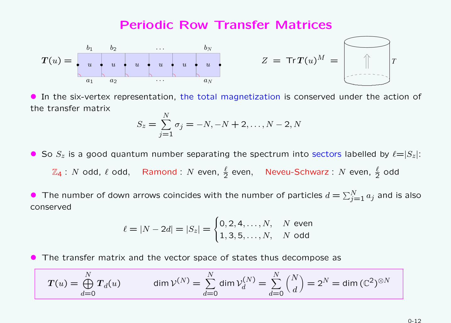
Periodic Row Transfer Matrices

T (u) = u u u u u u

a1 a2 · · · aN

b1 b2 · · · bN

Z = TrT (u)M = T

• In the six-vertex representation, the total magnetization is conserved under the action of

the transfer matrix

Sz =N∑

j=1

σj = −N,−N +2, . . . , N − 2, N

• So Sz is a good quantum number separating the spectrum into sectors labelled by ℓ=|Sz|:

Z4 : N odd, ℓ odd, Ramond : N even, ℓ2 even, Neveu-Schwarz : N even, ℓ

2 odd

• The number of down arrows coincides with the number of particles d =∑N

j=1 aj and is also

conserved

ℓ = |N − 2d| = |Sz| =

0,2,4, . . . , N, N even

1,3,5, . . . , N, N odd

• The transfer matrix and the vector space of states thus decompose as

T (u) =N⊕

d=0

T d(u) dimV(N) =N∑

d=0

dimV(N)d =

N∑

d=0

(N

d

)

= 2N = dim(C2)⊗N

0-12

Free Energy, Residual Entropy and Hamiltonian

• The bulk partition function per site

ρ κ(u) = ρ exp(−fbulk(u))

can be obtained by solving the inversion relation κ(u)κ(−u) = cos2 u (Baxter 1982) or by

using the Euler-Maclaurin formula. This gives the bulk free energy

fbulk(u) = −∫ ∞

−∞sinhut sinh(π2 − u)t

t sinhπt cosh πt2

dt = 12 log 2− 1

π

∫ π/2

0log(cosec t+ sin2u)dt

• Setting ρ =√2 and u = π

4 gives the known (Fisher 1961) molecular freedom W and residual

entropy S of dimers on the square lattice

W = eS =√2exp(−fbulk(

π4)) = exp(2Gπ ) = 1.791622812 . . . , S = 2G

π = .583121808 . . .

where W and Catalan’s constant are

W =√2κ(π4) = lim

M,N→∞(ZM×N)

1MN , G = 1

2

∫ π/2

0log(1 + cosec t)dt = .915965594 . . .

• The quantum Hamiltonian is given by the logarithmic derivative of the transfer matrix

given by the u(1) symmetric XX model

H =d

dulogT (u)

∣∣∣∣u=0

= −N∑

j=1

ej = −N∑

j=1

(f†j fj+1 + f

†j+1fj)

0-13

Inversion Identities

• The free-fermion single row transfer matrix satisfies the inversion identities (Felderhof 73)

T (u)T (u+ λ) =(

cos2N u− sin2N u)

I, N odd

T d(u)T d(u+ λ) = (cosN u+ (−1)d sinN u)2I, N even

• To solve these functional equations we factorize the right side. For example, in the Z4

sector, this factorization yields

cos2N u− sin2N u =e−2Niu

22N−1

N∏

j=1

(

e2iu + iǫj tan(2j − 1π)

4N

)(

e2iu − iǫj tan(2j − 1π)

4N

)

, ǫj = ±1

• Sharing out the zeros between T(u) and T(u+ λ) gives 2N eigenvalues

T(u) = ǫ(−i)N/2e−Niu

2N−1/2

N∏

j=1

(

e2iu + iǫj tan(2j − 1)π

4N

)

, Z4: N, ℓ odd

where ǫ = (−1)(N−ℓ)/4.

• Similarly, the solution of the inversion identity in the N even sectors yields

T(u) =ǫR(−i)

N2 e−Niu

2N−1

N∏

j=1

(

e2iu + iǫj tan(2j−1)π

2N

)

, R: N, ℓ/2 even

T(u) =ǫNS(−i)

N2Ne−Niu

2N−1

N∏

j=1

j 6=N/2

(

e2iu + iǫj tanjπ

N

)

, NS: N even, ℓ/2 odd

0-14

Counting Rotated Periodic Dimer Configurations

• The exact counting of periodic dimer configurations on a finite M × N square lattice, in

the 45 degree rotated orientation, is given by

ZM×N = Tr T (N)(π4

)M

where we set ρ =√2 and u = λ

2 = π4.

• The explicit formulas are

ZM×N=

2MN+1N∑

s=−N+2;4

∑

∑Nj=1 ǫj=s

(−1)M(N−s)

4

N∏

j=1

cosM(

ǫjtj − π4

)

, N odd

2MNN∑

s=−Ns = 0 mod 4

∑

∑Nj=1 ǫj=−|s|

(−1)M(2N+s)

4

N∏

j=1

cosM(

ǫjtRj − π

4

)

+ 2MNN∑

s=−Ns = 2 mod 4

∑

∑Nj=1 ǫj=−|s|

(−1)M(2N+|s|+2)

4

N∏

j=1

cosM(

ǫjtNSj − π

4

)

, N even

where s = Sz, tj =(2j − 1)π

4N, tRj =

(2j − 1)π

2N, tNS

j =

jπN , j 6= N

2

0, j = N2

0-15

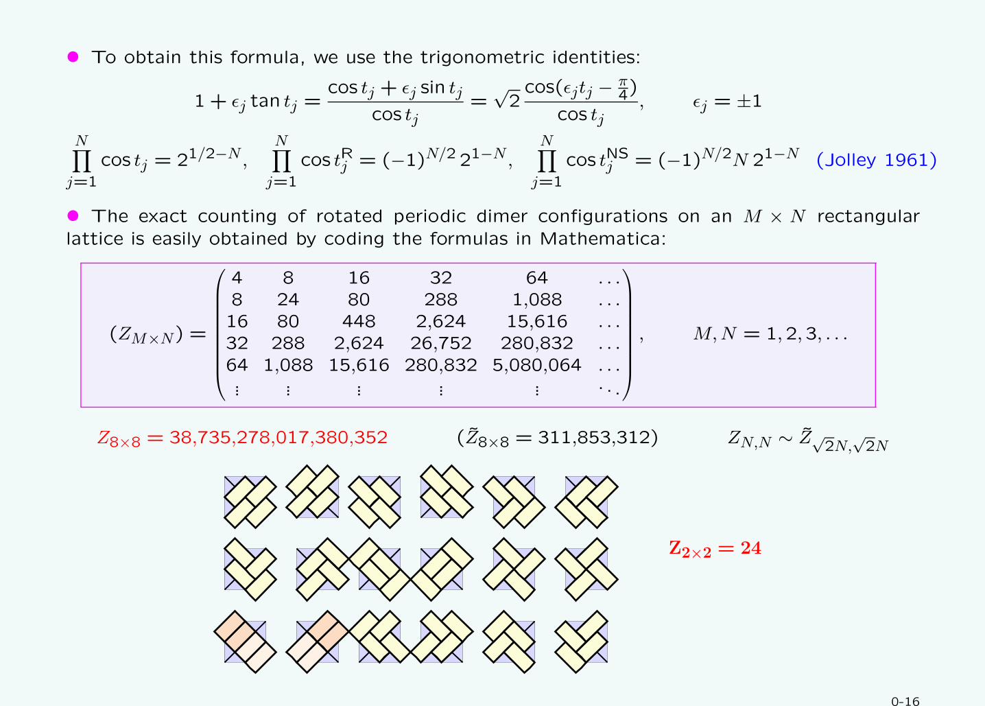
• To obtain this formula, we use the trigonometric identities:

1 + ǫj tan tj =cos tj + ǫj sin tj

cos tj=

√2cos(ǫjtj − π

4)

cos tj, ǫj = ±1

N∏

j=1

cos tj = 21/2−N ,N∏

j=1

cos tRj = (−1)N/2 21−N ,N∏

j=1

cos tNSj = (−1)N/2N 21−N (Jolley 1961)

• The exact counting of rotated periodic dimer configurations on an M × N rectangular

lattice is easily obtained by coding the formulas in Mathematica:

(ZM×N) =

4 8 16 32 64 . . .8 24 80 288 1,088 . . .16 80 448 2,624 15,616 . . .32 288 2,624 26,752 280,832 . . .64 1,088 15,616 280,832 5,080,064 . . .... ... ... ... ... . . .

, M,N = 1,2,3, . . .

Z8×8 = 38,735,278,017,380,352 (Z8×8 = 311,853,312) ZN,N ∼ Z√2N,

√2N

Z2×2 = 24

0-16

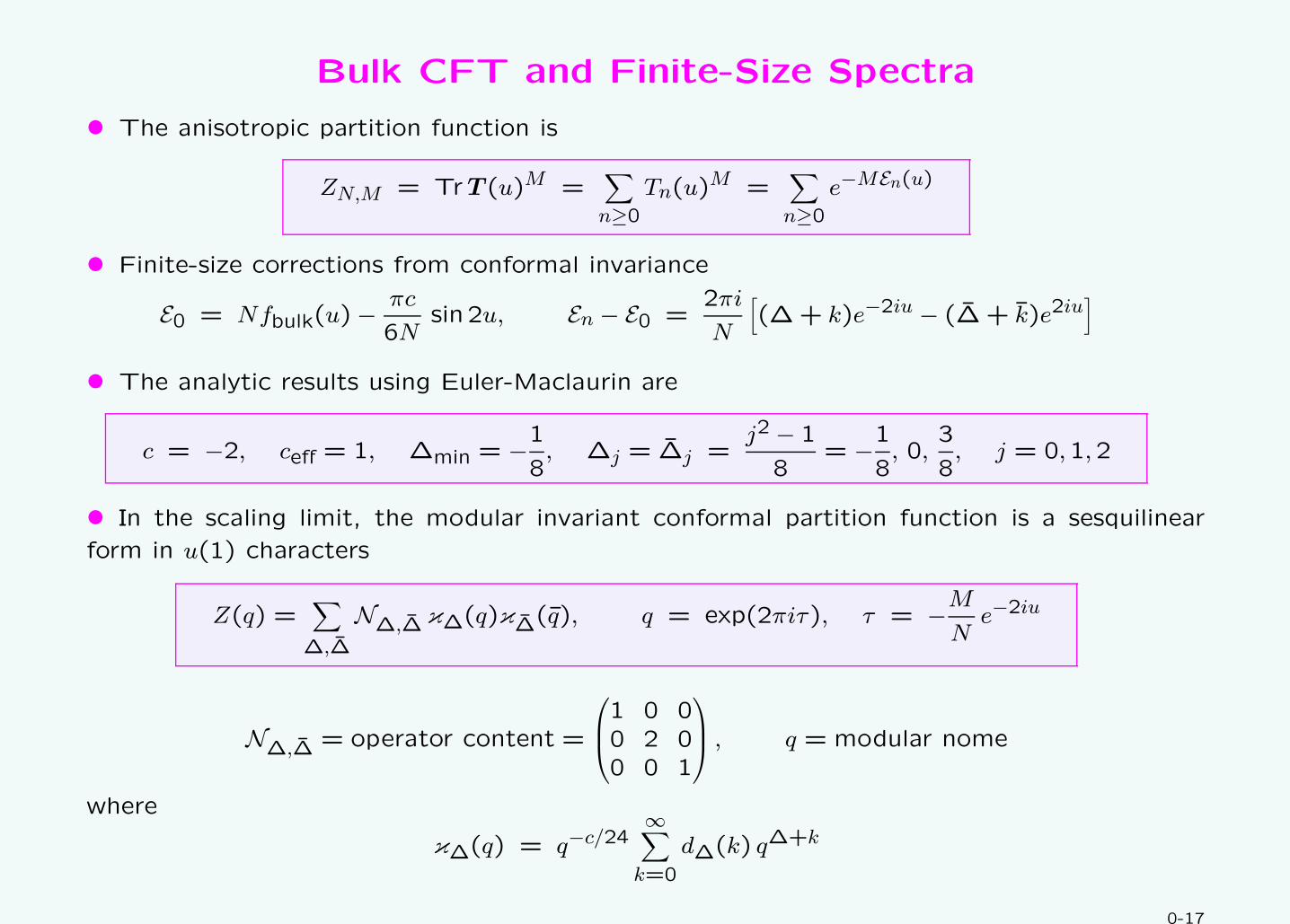
Bulk CFT and Finite-Size Spectra

• The anisotropic partition function is

ZN,M = TrT (u)M =∑

n≥0

Tn(u)M =

∑

n≥0

e−MEn(u)

• Finite-size corrections from conformal invariance

E0 = Nfbulk(u)−πc

6Nsin 2u, En − E0 =

2πi

N

[

(∆+ k)e−2iu − (∆ + k)e2iu]

• The analytic results using Euler-Maclaurin are

c = −2, ceff = 1, ∆min = −1

8, ∆j = ∆j =

j2 − 1

8= −1

8, 0,

3

8, j = 0,1,2

• In the scaling limit, the modular invariant conformal partition function is a sesquilinear

form in u(1) characters

Z(q) =∑

∆,∆

N∆,∆ κ∆(q)κ∆(q), q = exp(2πiτ), τ = −M

Ne−2iu

N∆,∆ = operator content =

1 0 00 2 00 0 1

, q = modular nome

where

κ∆(q) = q−c/24∞∑

k=0

d∆(k) q∆+k

0-17

Spectra: Sector-by-Sector

• Sector-by-sector Inversion Identity and patterns of zeros in complex u-plane: (ℓ = |Sz|)

T(u)T(u+ π2) =

cos2Nu− sin2Nu, N, ℓ odd,{

Z4 Sectors

(

cosNu+ (−1)(N−ℓ)/2 sinNu)2

, N, ℓ even,

Ramond (ℓ/2 even)

Neveu-Schwarz (ℓ/2 odd)

−π4

π4

π2

3π4

y5y4

y3

y2

y1

−y5−y4−y3

−y2

−y1

N, ℓ odd

−π4

π4

π2

3π4

y5y4

y3

y2

y1

−y5−y4−y3

−y2

−y1

N, ℓ even

• The y-ordinates of 1-strings uj and 1-string energies Ej are

yj = −12 log tan

Ejπ

N, Ej =

12(j −

12), j = 1,2, . . . , N ; Z4

j − 12, j = 1,2, . . . , N/2; Ramond

j, j = 1,2, . . . , N/2− 1; Neveu-Schwarz

0-18

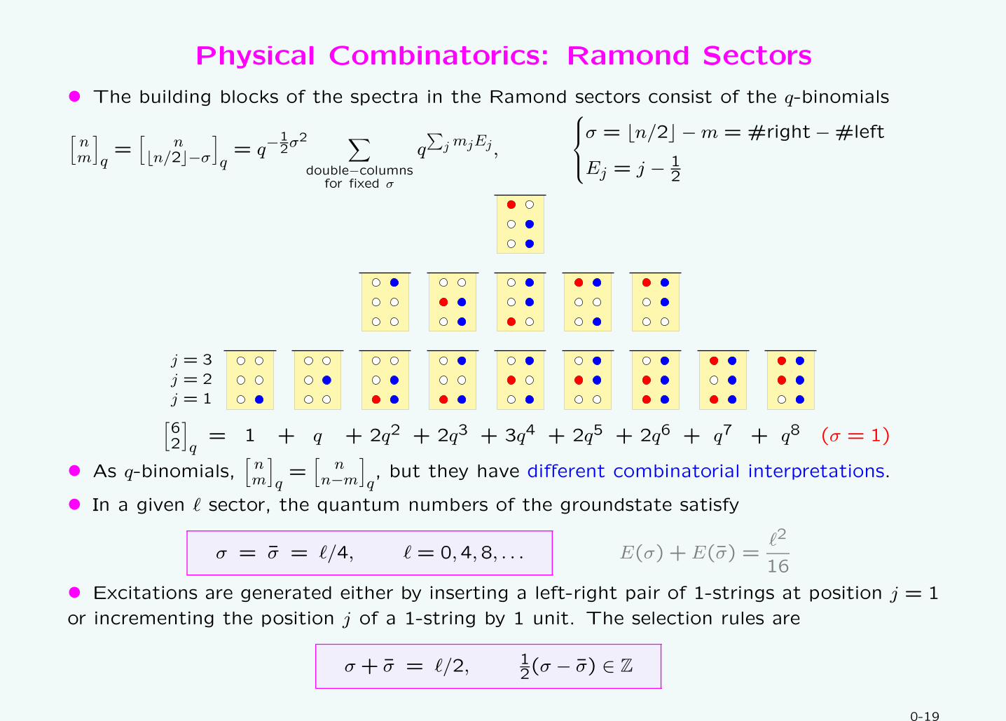
Physical Combinatorics: Ramond Sectors

• The building blocks of the spectra in the Ramond sectors consist of the q-binomials

[nm

]

q=

[n

⌊n/2⌋−σ

]

q= q−

12σ

2 ∑

double−columnsfor fixed σ

q∑

j mjEj ,

σ = ⌊n/2⌋ −m = #right−#left

Ej = j − 12

[62

]

q= + + + + + + + +1 q 2q2 2q3 3q4 2q5 2q6 q7 q8 (σ = 1)

j = 1

j = 2

j = 3

• As q-binomials,[nm

]

q=

[n

n−m

]

q, but they have different combinatorial interpretations.

• In a given ℓ sector, the quantum numbers of the groundstate satisfy

σ = σ = ℓ/4, ℓ = 0,4,8, . . . E(σ) + E(σ) =ℓ2

16

• Excitations are generated either by inserting a left-right pair of 1-strings at position j = 1

or incrementing the position j of a 1-string by 1 unit. The selection rules are

σ + σ = ℓ/2, 12(σ − σ) ∈ Z

0-19

Physical Combinatorics: Neveu-Schwarz Sectors

• The building blocks of the spectra in the Neveu-Schwarz sectors consist of the q-binomials

[nm

]

q=

[n

⌊n/2⌋−σ

]

q= q−

12σ(σ+1)

∑

double−columnsfor fixed σ

q∑

j mjEj ,

σ = ⌊n/2⌋ −m, #right−#left = σ, σ +1

Ej = j

[72

]

q= + + + + + + + + + +1 q 2q2 2q3 3q4 3q5 3q6 2q7 2q8 q9 q10 (σ = 1)

j = 1

j = 2

j = 3

• As q-binomials,[nm

]

q=

[n

n−m

]

q, but they have different combinatorial interpretations.

• In a given ℓ sector, the quantum numbers of the groundstate satisfy

σ = σ = (ℓ− 2)/4, ℓ = 2,6,10, . . .

(

E(σ) + E(σ) =ℓ2 − 4

16

)

• Excitations are generated either by inserting a right or left 1-string at position j = 1 or

incrementing the position j of a 1-string by 1 unit. The selection rules are

σ + σ = (ℓ− 2)/2, 12(σ − σ) ∈ Z

0-20

Finitized Modular Invariant Partition Function (N, ℓ Even)

• Ramond sectors (ℓ/2 even)

Z(N)ℓ (q) = (qq)−c/24

∑

k∈Zq∆2k+ℓ/2

[

2⌊N+24 ⌋

⌊N+2−ℓ4 ⌋−k

]

q

q∆2k−ℓ/2

[

2⌊N4 ⌋⌊N−ℓ

4 ⌋+k

]

q

• Neveu-Schwarz sectors (ℓ/2 odd)

Z(N)ℓ (q) = (qq)−c/24

∑

k∈Zq∆2k+ℓ/2

[

2⌊N4 ⌋+1

⌊N+2−ℓ4 ⌋−k

]

q

q∆2k−ℓ/2

[

2⌊N+24 ⌋−1

⌊N−ℓ4 ⌋+k

]

q

• Finitized Modular Invariant Partition Function

ZN(q) = Z(N)0 +2

ℓ≤N∑

ℓ∈4NZ(N)ℓ (q) + 2

ℓ≤N∑

ℓ∈4N−2

Z(N)ℓ (q)

We find that

ZN(q) = 12(qq)

− c24−

18

[ ⌊N+24 ⌋∏

n=1

(1 + qn−12)2

⌊N4 ⌋∏

n=1

(1 + qn−12)2 +

⌊N+24 ⌋∏

n=1

(1− qn−12)2

⌊N4 ⌋∏

n=1

(1− qn−12)2

]

+2(qq)−c24

⌊N4 ⌋∏

n=1

(1 + qn)2⌊N−2

4 ⌋∏

n=1

(1 + qn)2

0-21

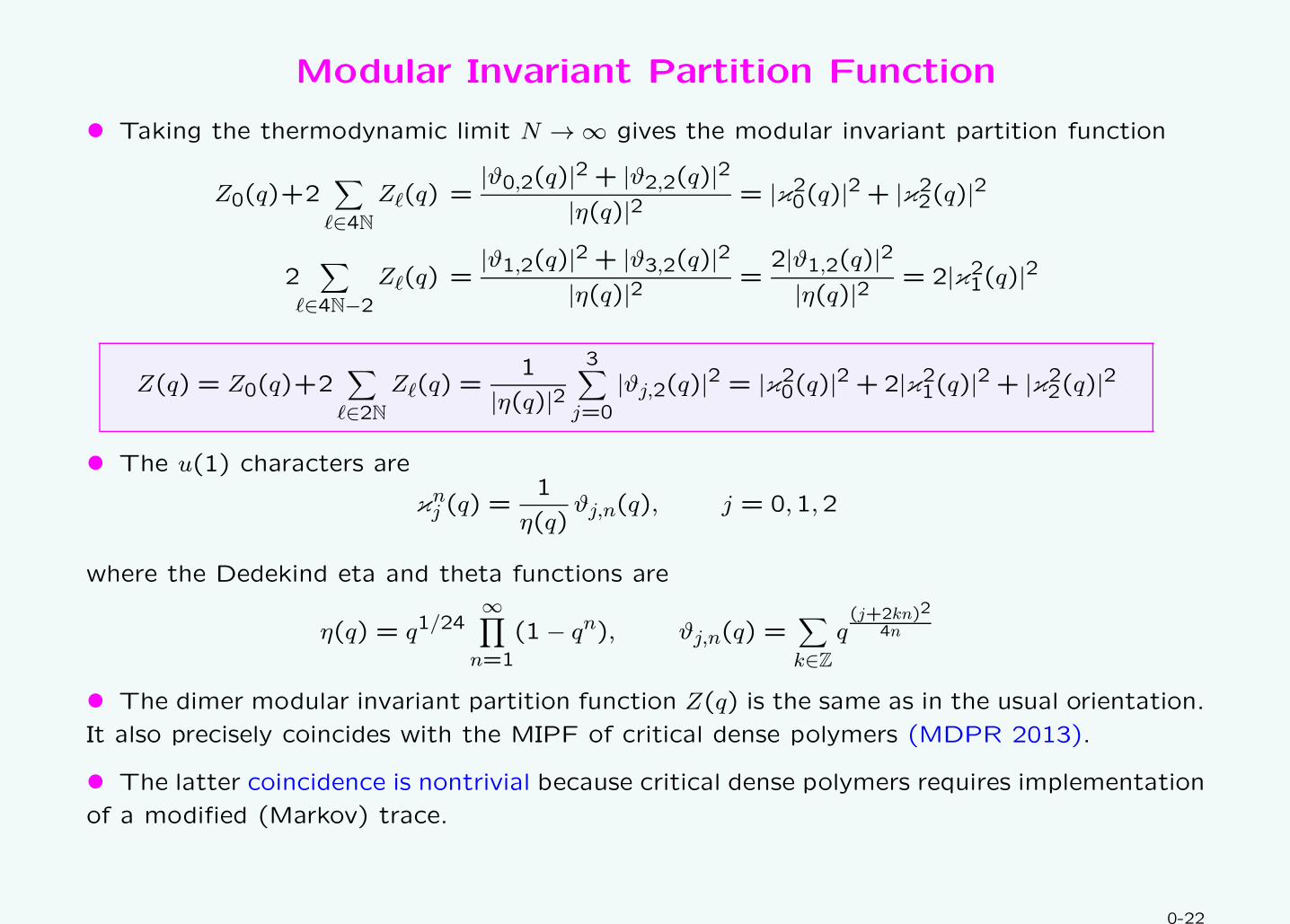
Modular Invariant Partition Function

• Taking the thermodynamic limit N → ∞ gives the modular invariant partition function

Z0(q)+2∑

ℓ∈4NZℓ(q) =

|ϑ0,2(q)|2 + |ϑ2,2(q)|2|η(q)|2 = |κ2

0(q)|2 + |κ22(q)|2

2∑

ℓ∈4N−2

Zℓ(q) =|ϑ1,2(q)|2 + |ϑ3,2(q)|2

|η(q)|2 =2|ϑ1,2(q)|2|η(q)|2 = 2|κ2

1(q)|2

Z(q) = Z0(q)+2∑

ℓ∈2NZℓ(q) =

1

|η(q)|23∑

j=0

|ϑj,2(q)|2 = |κ20(q)|2 +2|κ2

1(q)|2 + |κ22(q)|2

• The u(1) characters are

κnj (q) =

1

η(q)ϑj,n(q), j = 0,1,2

where the Dedekind eta and theta functions are

η(q) = q1/24∞∏

n=1

(1− qn), ϑj,n(q) =∑

k∈Zq(j+2kn)2

4n

• The dimer modular invariant partition function Z(q) is the same as in the usual orientation.

It also precisely coincides with the MIPF of critical dense polymers (MDPR 2013).

• The latter coincidence is nontrivial because critical dense polymers requires implementation

of a modified (Markov) trace.

0-22

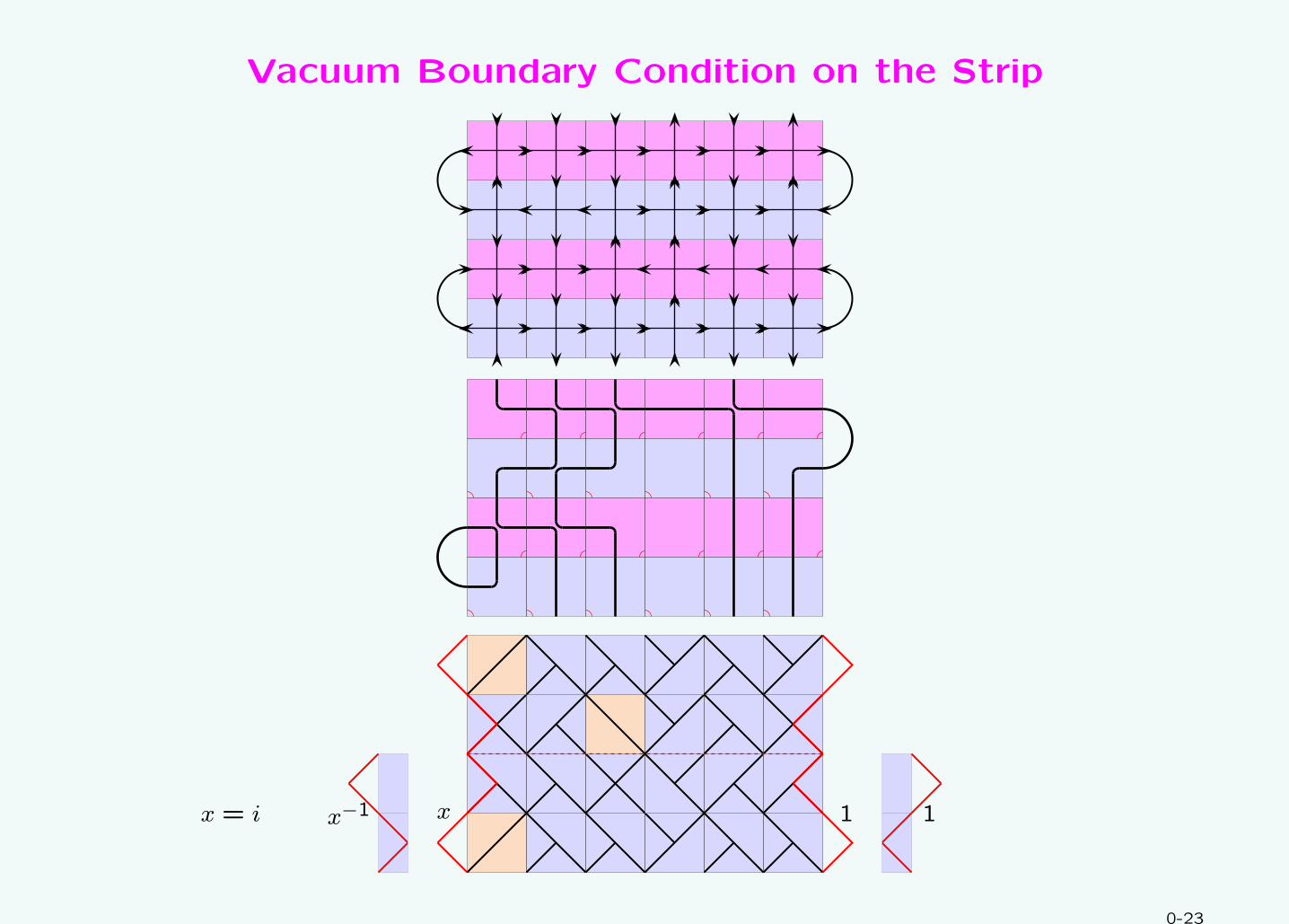
Vacuum Boundary Condition on the Strip

xx−1x = i 1 1

0-23

Jordan Cells

• The Hamiltonian for dimers with the (r, s) = (1,1) vacuum boundary condition (no seam)

on the strip coincides with the Uq(sl(2))-invariant u(1) symmetric XX Hamiltonian

H = −N−1∑

j=1

ej = −12

N−1∑

j=1

(σxj σxj+1 + σ

yjσ

yj+1)−

12i(σ

z1 − σzN)

= −N−1∑

j=1

(f†j fj+1 + f

†j+1fj)− i(f

†1f1 − f

†NfN)

where σx,y,zj are Pauli matrices and fj = σxj −iσ

yj , f

†j = σxj +iσ

yj . This Hamiltonian is manifestly

not Hermitian but the eigenvalues are real (MDRRSA2016).

• The Jordan canonical forms for N = 2 and N = 4 are

0⊕(

0 10 0

)

⊕ 0

0⊕(0 10 0

)

⊕ 0⊕ 0⊕(0 10 0

)

⊕ 0⊕ (−√2)⊕

(−√2 1

0 −√2

)

⊕ (−√2)⊕

√2⊕

(√2 1

0√2

)

⊕√2

• In the continuum scaling limit, the Hamiltonian gives the Virasoro dilatation operator L0.

Assuming that the Jordan cells persist in this scaling limit, the representation is reducible yet

indecomposable and so, as a CFT, dimers is logarithmic!

• For dimers with (1, s) boundary conditions the conformal weights are

∆1,s =(2− s)2 − 1

8= 0,−1

8,0,

3

8,1,

15

8, . . . s = 1,2,3,4,5,6, . . .

0-24

Summary and Outlook

• The anisotropic dimer model on the square lattice, with 45 degree rotated dimers, has

been solved exactly on a torus using Yang-Baxter integrability.

• Explicit formulas are found for the counting of dimer configurations on a periodic M ×N

rectangular lattice.

• The modular invariant partition function precisely coincides with critical dense polymers.

• Since ∆1,2 = −18 and the six-vertex model with λ = π

2 on the strip with vacuum boundary

conditions exhibits Jordan cells (e.g. Gainutdinov, Nepomechie et al 2015), we argue that

dimers is nonunitary and logarithmic with central charge c = −2 and ceff = 1.

• Yang-Baxter methods can now be applied to study dimers on a strip with many different

boundary conditions. General (r, s) boundary conditions are under construction (with

Rasmussen). Some insight may also be gained for Aztec diamonds and the six vertex model

with domain wall boundary conditions.

• The inversion identity is the Y -system for dimers. The analogous Y -system for critical bond

percolation can be solved analytically (Morin-Duchesne, Klumper, Pearce 2017). Remarkably,

the same two-column “symplectic binomial” building blocks reappear in the patterns of zeros.

0-25

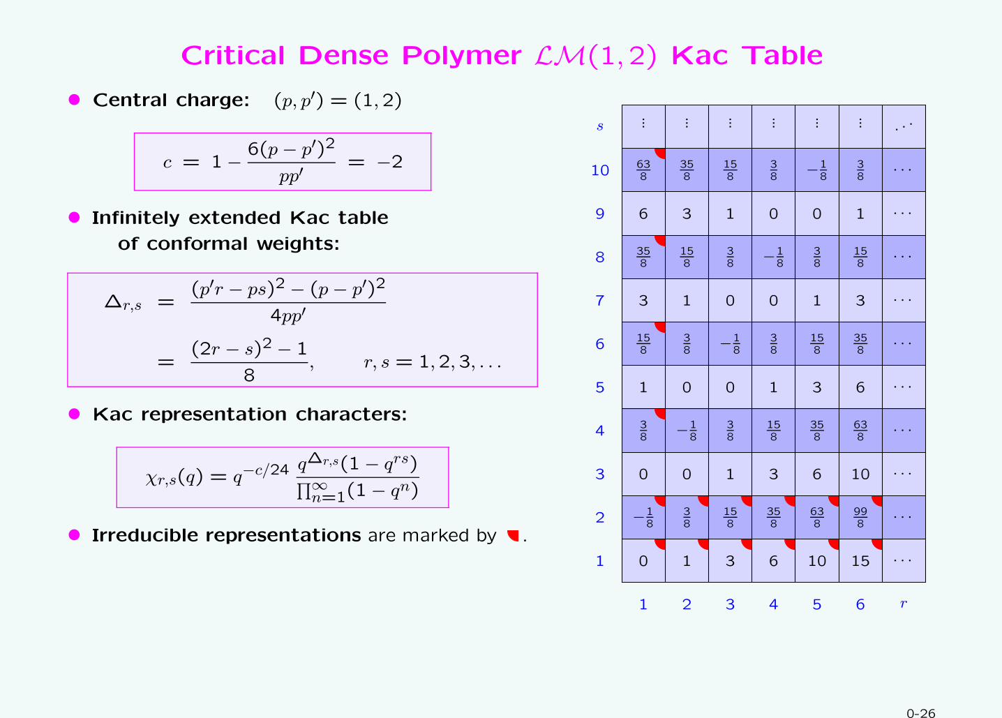
Critical Dense Polymer LM(1,2) Kac Table

• Central charge: (p, p′) = (1,2)

c = 1− 6(p− p′)2

pp′= −2

• Infinitely extended Kac table

of conformal weights:

∆r,s =(p′r − ps)2 − (p− p′)2

4pp′

=(2r − s)2 − 1

8, r, s = 1,2,3, . . .

• Kac representation characters:

χr,s(q) = q−c/24 q∆r,s(1− qrs)∏∞n=1(1− qn)

• Irreducible representations are marked by .

... ... ... ... ... ... . . .

638

358

158

38

−18

38

· · ·

6 3 1 0 0 1 · · ·

358

158

38

−18

38

158

· · ·

3 1 0 0 1 3 · · ·

158

38

−18

38

158

358

· · ·

1 0 0 1 3 6 · · ·

38

−18

38

158

358

638

· · ·

0 0 1 3 6 10 · · ·

−18

38

158

358

638

998

· · ·

0 1 3 6 10 15 · · ·

1 2 3 4 5 6 r

1

2

3

4

5

6

7

8

9

10

s

0-26

Critical Dense Polymers

• Logarithmic Minimal Models: Yang-Baxter integrable loop models on the square

lattice. Face operators defined in diagrammatic planar Temperley-Lieb algebra (Jones1999)

X(u) = u = sin(λ− u) + sinu

1 ≤ p < p′ coprime integers, λ =(p′ − p)π

p′= crossing parameter

u = spectral parameter, β = 2cosλ = nonlocal loop fugacity

• Critical Dense Polymers: (p, p′) = (1,2), λ =π

2

Z =∑

loop configs

cosN1 u sinN2 u,

β = 0 ⇒ no closed loops ⇒ space filling dense polymer ⇒ dSLEpath = 2− 2∆1,1 = 2

• There are no local degrees of freedom only nonlocal degrees of freedom in the form of

extended polymer segments!

0-27