ROEVER COLLEGE OF ENGINEERING & TECHNOLOGY

Elambalur, Perambalur – 621 212.

DEPARTMENT OF METHAMATICS

QUESTION BANK

MA 2264 – NUMERICAL METHODS

UNIT – I

SOLUTION OF EQUATIONS AND EIGEN VALUE PROBLEMS

PART – A 1. What is the iterative formula of Newton – Raphson Method?

2. What is the order of convergence and the convergence condition for Newton’s Raphson method?

3. Derive a formula to find the value of N where N > 0, using Newton – Raphson method.

4. Find an iterative formula to find the reciprocal of a given number N( N ≠ 0).

4. What are the merits of Newton’s method of Iteration?

5. When should we not use Newton Raphson?

6. State the sufficient condition for the existence and uniqueness of fixed point iteration.

7. Write down the order of convergence and the condition for convergence of fixed point iteration method.

9. What do you mean by the order of convergence of an iterative method for finding the root of the equation f(x) = 0.

8. Give two direct methods to solve a system of linear equations.

9. What are the advantages of iterative methods over direct methods for solving a system of linear equations?

10. Give two indirect methods to solve a system of linear equations.

11. State any two difference between direct and iterative methods for solving system of equations.

12. State the principle used in Gauss – Jordan method.

13. Compare Gaussian elimination and Gauss – Jordan Methods in solving the linear system

A X B .

14. Compare Gauss - elimination with Gauss seidal method.

16. Solve the equations x + 2y = 1 and 3x – 2y = 7 by Gauss – Elimination method.

17. using Gauss elimination method solve: 5x + 4y = 15, 3x + 7y = 12.

15. Compare Gauss – Jacobi & Gauss Seidal Methods.

16. Solve by Gauss–Jordan Method the following system of equations 2x1 + x2 = 3, x1 + 2x2 = 3.

17. Find inverse of 1 3

2 7A

by Gauss Jordan Method.

18. Write the sufficient condition for Gauss – seidal Method to converge.

19. Define eigen value and eigen vector.

20. State the basic principle involved for finding A-1 by Gauss – Jordan Method?

21. How will you find the smallest eigenvalue of a square matrix A?

22. If the eigen values of A are 1, 3, 4 then the dominant eigenvalue of A is ------------.

23. The power Method will work satisfactorily only if A has a -------------eigen value.

25. What is the use fo Power method?

PART – B

Method – I– NewtoN’s RaphsoN:

1. Find the root of 4 0xx e that lies between 2 and 3 by Newton’s Method.

2. *Find by Newton’s iterative formula for the reciprocal of a number N and hence find the value of 1/23,

correct to five decimal places.

3. (i)Solve by Newton – Raphson Method the Equation xsinx + cosx = 0, correct to four decimal

places. (ii) *Solve by N – R method 10log 1.2 0x x .

4. Find by Newton’s Method, the real root of the equations (i)* 3x = cosx +1. And (ii) cosxxe x .

5. Establish the formula to find the square root of N, using Newton – Raphson Method. Hence

find the square root of (i)15, (ii)11, (iii) 5 correct to 3 decimal places.

6. Prove the quadratic convergence of Newton Raphson Method. Find a +ve real root of

f(x) = x3 – 5x + 3 = 0, using this method.

7. Find the +ve real root of (i) x3 – 2x + 0.5 = 0 and (ii) x4 – x – 10 = 0using Newton – Raphson Method correct

to 3 decimal places.

8. Obtain the +ve of 2x3 – 3x - 6 = 0 that lies between 1 and 2 by using Newton – Raphson method.

9. Find by Newton’s method, the root of ex = 4x near x = 2, correct to four decimal places.

Method – II – FIXED POINT ITERATION : 1. Find a real root of the equation cosx = 3x – 1 correct to 5 decimal places by fixed point iteration method.

2. *Solve 3 0xe x by the method of fixed point iteration.

3. Find the –ve root of the equation x3 – 2x + 5 = 0.

4. Use the method of fixed point iteration to solve the equation 103 log 6x x .

5. Solve the following by iteration method.

(i) 3x – cosx - 2 = 0.

(ii) 102 log 7x x .

Method – II – GAUSS – JORDAN :

1. Using Gauss – Jordan method, solve the following system of equations

(i) 2x – y + 3z = 8, x + 2y + z = 4 , 3x + y –z = 0 and (ii) 10x + y + z = 12, 2x + 10y + z = 13, x + y + 5z = 7.

2. Solve by Gauss – Jordan Method the following system

(i) 10x + y – z = 11.19 * (ii) 10x + y + z = 12

x + 10y + z = 20.08 x + 10y + z = 12

-x +y + 10z = 35.61. x + y + 10z = 12.

3. Solve the following equations by Gauss Jordan method.

(i) x + y + z = 9, 2x – 3y + 4z = 13, 3x + 4y + 5z = 40.

(ii) 2x + y + 4z = 12, 8x – 3y + 2z = 20, 4x + 11y – z = 33.

(iii)5x – y = 9; - x + 5y – z = 4; - y + 5z = -6.

Method – III – GAUSS - ELIMINATION :

1. Solve the given system of equations by Gaussian elimination method

-x1 +x2 + 10x3 = 35.61

10x1 + x2 – x3 = 11.19

x1 + 10x2 + x3 = 20.08.

2. Solve the system of equations by Gauss elimination method.

(i) 10x – 2y + 3z = 23 (ii) 3.15x -1.96y + 3.85z = 12.95

2x + 10y – 5z = -33 2.13x + 5.12y – 2.89z = -8.61

3x – 4y + 10z = 41. 5.92x + 3.05y +2.15z = 6.88.

Method – IV – Inverse of the matrix:

1. Find the inverse of (i)

4 1 2

2 3 1

1 2 2

A

, (ii) *3 1 1

15 6 5

5 2 2

A

, (iii)

8 1 3

5 1 2

10 1 4

A

using Gauss -

Jordan method.

2. Using Gauss – Jordan Method find the inverse of the following matrices

1 1 3 4 1 2

1 3 3 2 3 1

2 4 4 1 2 2

i A ii A

(iii)3 1 2

2 3 1

1 2 1

A

(iv) *2 2 6

2 6 6

4 8 8

A

1 1 1

( ) 4 3 1

3 5 3

v A

.

1 1 2

( ) 1 2 3

2 3 1

vi A

1 2 1

( ) 4 1 0

2 1 3

vii A

, (viii)

0 1 2

1 2 3

3 1 1

A

(ix)

1 2 6

2 5 15

6 15 46

A

Method – V – Gauss – Jacobi:

1. Solve by Gauss – Jacobi Method, the following equation

(i) 4x1 + x2 + x3 = 6 (ii) **8x -3y +2z = 20

x1 + 4x2 + x3 = 6 4x + 11y – z = 33

x1 + x2 + 4x3 = 6. 6x + 3y + 12z = 35

2. Solve by Gauss – Jacobi method the equations

20x + y – 2z = 17, 3x + 20y – z = -18, 2x – 3y + 20z = 25.

Method – VI – Gauss – seidal:

1. Solve the following system of equations by Gauss – Seidal method

(i) *4x + 2y +z = 14, x + 5y – z = 10, x + y + 8z = 20.

(ii) 2x + 10y + z = 13, 10x + y + z = 12, x + y + 5z = 7.

(iii)* 20x + y – 2z = 17, 3x + 20y – z = -18, 2x – 3y + 20z = 25.

(iv)* x + y + 54z = 110, 27x + 6y – z = 85, 6x + 15y + 2z = 72.

(v) 8x -3y +2z = 20, 4x + 11y – z = 33, 6x + 3y + 12z = 35.

(vi)9x – y + 2z = 9, x + 10y – 2z = 15, 2x – 2y - 13z = -17.

(vii) **10x + 2y + z = 9, x + 10y – z = -22, -2x + 3y + 10z = 22.

2. Solve by Gauss – Seidal method

(i) 6x – 3y + z = 11 (ii) 28x + 4y – z = 32 (iii) 6x -3y + z = 1 (iv) 28x + 4y – z = 32

x + 3y + 10z = 24 2x + y – 8z = -15 2x + y -8z = -15 x + 3y + 10z = 24

2x + 17y + 4z = 35 x – 7y + z = 10. x – 7y + z = 10. 2x + 17y + 4z = 35

3. Using Gauss Seidal Method, solve the following system start with x = 1, y = -2, z = 3

x + 3y + 52z = 173.61

x – 27y + 2z = 71.81

41x – 2y + 3z = 65.46

4. Solve by Gauss – Seidal iteration the given system of equations starting with (0, 0, 0) as solution. Do 5

iteration only 4x – x2 –x3 = 2, - x1 + 4x2 – x4 = 2, -x1 + 4x3 – x4 = 1, - x2 –x3 + 4x4 = 1.

Method – VII – EIGEN VALUE OF A MATRIX BY Power method

1. **Find the Largest eigenvalues of 5 0 1

0 2 0

1 0 5

A

by power method.

2. Determine the Largest eigen value and the corresponding eigenvector of the matrix using the power

method 2 1 0

1 2 1

0 1 2

A

.

3. Find the dominant Eigen value and the corresponding Eigen vector of

1 6 1

1 2 0

0 0 3

A

Using power method with the initial Eigen vector 0

1

1

1

X

.

4. Solve by power method to find the dominant Eigen value for the matrix

1 1 3

1 5 1

3 1 1

.

5. Find the numerically largest eigenvalues and the corresponding Eigen vector using power method, given

(i)5 4 3

10 8 6

20 4 22

A

, (ii) *1 3 1

3 2 4

1 4 10

A

. Starting vector is ( 1, 1, 1)T.

6. Obtain by the power method, the dominant eigen value and the corresponding eigen vector Correct to two

decimal places for the matrix 2 2 2 1

2 / 3 5 / 3 5 / 3 0

1 5 / 2 11/ 2 0

taking

as the initial approximation to the eigen vector.

7. *Find the numerically largest eigenvalues and the corresponding Eigen vector using power method, given

25 1 2

1 3 0

2 0 4

A

. Starting vector is ( 1, 0, 0)T.

8. Find the numerically largest eigenvalues and the corresponding Eigen vector using power method, given

(i) 1 2 3

0 4 2

0 0 7

A

, (ii) 15 4 3

10 12 6

20 4 2

A

Method – VIII – EIGEN VALUE OF A MATRIX BY JACOBI method 1. Find all the Eigen values and Eigen vectors of the following matrix by using Jacobi method.

(i) 1 2 2

2 3 2

2 2 1

A

, (ii)

2 0 1

0 2 0

1 0 2

A

(iii) 5 0 1

0 2 0

1 0 5

A

(iv)

4 1 1

1 1 2

1 2 1

A

(v)

6 2 2

2 3 1

2 1 3

A

(vi)

3 1 1

1 5 1

1 1 3

A

(vii)

1 0 0

0 3 1

0 1 3

A

UNIT – II

INTERPOLATION AND APPROXIMATIONS

PART – A 1. State Lagrange’s interpolation formula.

2. What is the assumption we make when Lagrange’s formuls is used?

3. Use Lagrange’s formula, to find the quadratic polynomial that takes these values.

X: 0 1 3

Y: 0 1 0 Then find y(2).

4. Explain briefly interpolation.

5. State the order of convergence of cubic spline.

6. State the properties of cubic spline.

7.* Derive Newton’s forward and backward difference formula. (OR) State Gregory – Newton forward

difference interpolation formula.

8. State Newton’s forward difference formula for equal intervals.

8. Obtain the divided difference table for the following data

x -1 0 2 3

f(x) -8 3 1 12

9. Fit a polynomial which takes the following values:

10. Using Lagrange’s formula, find the polynomial to the given data.

10. What do you understand by inverse interpolation?

11. What is the nature of nth divided differences of a polynomial of nth degree?

12. Find the second divided difference with arguments a, b, c if f(x) = 1/x.

13. Form the divided difference table for the data (0, 1), (1, 4), (3, 40) and (4, 85).

14. **Define a cubic spline S(x) which is commonly used for interpolation.

15. If y(x) = y, I = 0, 1, …, n write down the formula for the cubic spline polynomial y(x), valid in xi-1< x < xi.

16. What is meant by Natural cubic spline?

17. What in the error in Newton’s forward interpolation formula?

18. When to use Newton’s forward interpolation and when to use Newton’s backward interpolation?

19. Find the divided difference of f(x) = x2 + x + 2 for the arguments 1, 3, 6, 11.

20. Find the divided difference of f(x) = x3 – x2 + 3x + 8 for the arguments 0, 1, 4, 5.

21. Find the second divided difference with arguments a, b, c if f(x) = 1/x.

20. Show that 3 1 1

bcd a abcd

.

21. What is inverse interpolation?

PART – B

Method – I – LagRaNge’s iNteRpoLatioN foRmuLa:

1. Using Lagrange’s interpolation formula, find x corresponding to

y = 85 given

2. Given the values

x 0 1 2

Y 1 2 1 x 0 1 3

Y 5 6 50

x 2 5 8 14

y 94.8 87.9 81.3 68.7

x 5 7 11 13 17

f(x) 150 392 1452 2366 5202

Evaluate f(9), using (i) Lagrange’s formula (ii) Newton’s divided difference formula.

3. Find f(x) as a polynomial in x from the given data and find f(8) and f(6).

4. **Find y(40) from the following data using Lagrange’s interpolation formula y(30) = 148, y(35) = 96,

y(45) = 68 and y(55) = 34.

5. Fit a Lagrange’s interpolating polynomial y = f(x) and find f(5).

6. Find the polynomial f(x) by using Lagrange’s formula and hence find f(3).

7. ***Given the values Find f(27) by using Lagrange’s interpolation formula.

8. Using Lagrange’s interpolation formula fit a polynomial to the following data: And hence find y at

x = 1.5

9. The following table gives certain corresponding values of x and log10x. Compute the value of

log10323.5, by using Lagrange’s interpolation formula.

10. Use Lagrange’s interpolating formula to fit a polynomial to the given data f(-1) = -8, f(0) = 3,

f(2) = 1 and f(3) = 12. Hence find the value of f(1).

11. Use Lagrange’s method to find log10656, given that log10654 = 2.8156, log10658 = 2.8182, log10659 = 2.8189

and log10661 = 2.8202.

Method – II - NewtoN’s divided diffeReNce method:

1. **Using Newton’s divided difference formula, find f(8) for the given

data:

2. Determine f(x) as a polynomial in x for the following data, using Newton’s

divided difference formula. Also find f(2).

3. Using Newton’s divided difference formula find the equation y = f(x) of

least degree and passing through the points (-1, -21), (1, 15), (2, 12), (3, 3). Find also y at x = 0.

4. From the following table find f(x), by Newton’s divided difference

interpolation formula.

5. Use Newton’s divided difference formula, find u(3) given u(1) = -26, u(2) = 12, u(4) = 256,

u(6) = 844.

6. Given the values

Evaluate f(9) using Newton’s divided difference formula

7. If f(0) = f(1) = f(2) = -12, f(4) = 0, f(5) = 600 and f(7) = 7308, find a polynomial that satisfies this

data using Newton’s divided difference interpolation formula. Hence, find f(6).

x 3 7 9 10

f(x) 168 120 72 63

x 1 3 4 6

y=f(x) -3 0 30 132

x 0 1 2 3

f(x) 2 3 12 147

x 14 17 31 35

f(x) 68.5 64 44 39.5

x -1 0 2 3

y -8 3 1 12

x 321.0 322.8 324.2 325.0

Log10x 2.50651 2.50893 2.51081 2.51188

x 4 5 7 10 11 13

y 48 100 294 900 1210 2028

x -4 -1 0 2 5

f(x) 1245 33 5 9 1335

x 0 2 3 4 6 7

y 0 8 0 -72 0 1008

x 5 7 11 13 17

y 150 392 1452 2366 5202

x 3 7 9 10

8. Using divided difference, find f(x) as a polynomial in x from the given data:

9. Use Newton’s divided difference formula to find f(5) from the following data:

10. *Use Newton’s divided difference formula to find f(x) from the following data and hence find f(4).

11. Use Newton’s divided difference formula to find f(x) from the following data

Method – III – Cubic spline approximation:

1. ****Find the cubic spline approximation for the function y = f(x) from the data,

given that '' ''

0 3 0y y .

2. Fit the 4 points by the cubic splines, using the conditions '' ''

0 3 0y y .

3. Find the natureal cubic spline to fit the data.

Hence find f(0.5) and f(1.5).

4. Fit a natural cubic spline for the following data

5. Fit a cubic spline curve for the points (2, 11), (3, 49) and (4, 123). Hence find y(2.5) and '(3.5)y , assume that

''(2) 0y and

''(4) 0y .

6. Fit the cubic spline for the data: Hence evaluate y(1.5)

7. The following values of x and y are given: Find the cubic splines and evaluate

y(1.5) .

8. Fit the straight line for the data.

9. Using cubic spline, compute y(1.5) from the given data.

Method – IV – Newton Forward and backward difference:

1. Find y at x = 84 using backward difference for the given data.

2. The following are data from the steam table. Find the pressure at temperature t = 1750C and t = 1420C.

Using Newton’s Backward and Forward difference Formula.

f(x) 168 120 72 63

x 0 2 3 4 7

f(x) 4 26 58 112 466

x 0 1 2 5

f(x) 2 3 12 147

x 1 2 7 8

y 1 5 5 4

x -1 0 1 2

y -1 1 3 35

i 0 1 2 3

x 1 2 3 4

y 1 5 11 8

x 0 1 2

f(x) -1 3 29

x 0 1 2 3

y 1 4 0 -2

x 1 2 3

y -6 -1 16

x 1 2 3 4

y 1 2 5 11

x 0 1 2 3

y 1 2 9 28

x 1 2 3

y -8 -1 18

x 40 50 60 70 80 90

y 184 204 226 250 276 304

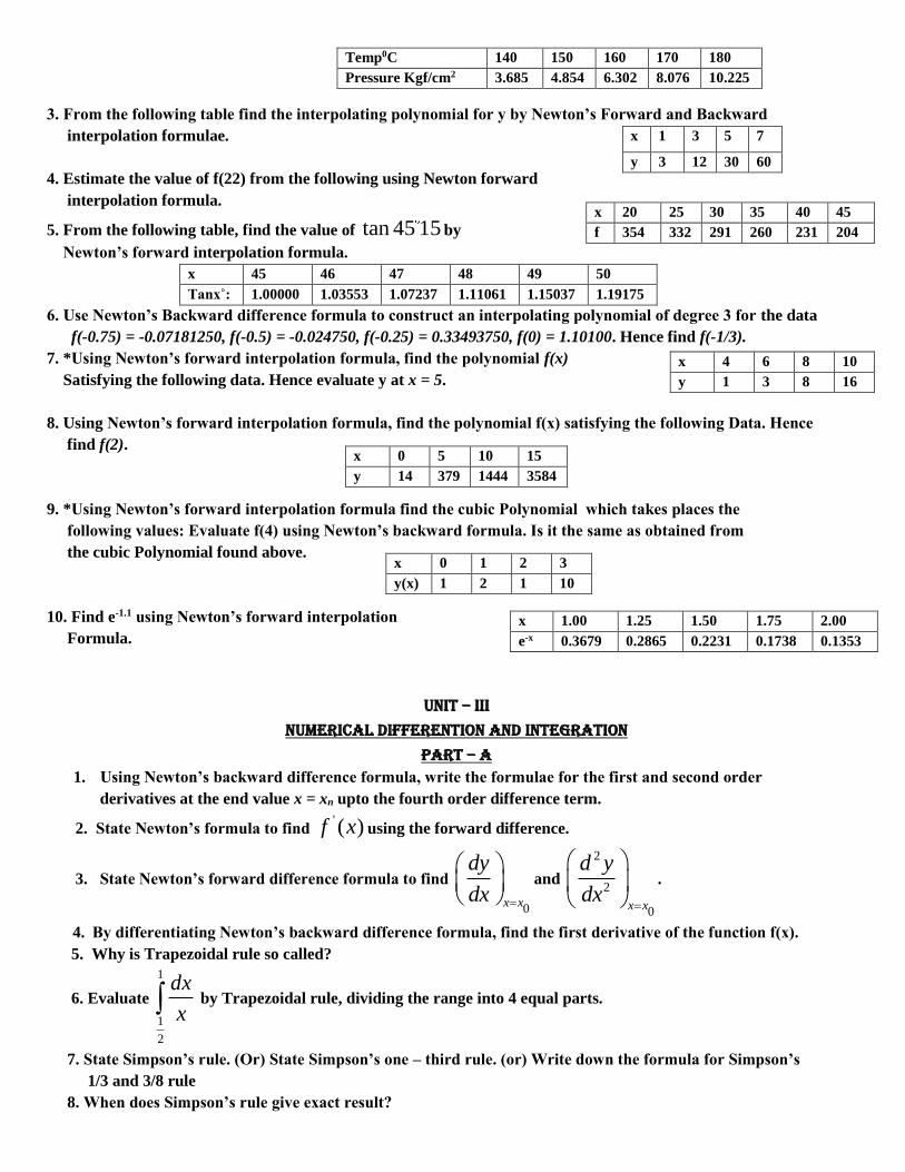
3. From the following table find the interpolating polynomial for y by Newton’s Forward and Backward

interpolation formulae.

4. Estimate the value of f(22) from the following using Newton forward

interpolation formula.

5. From the following table, find the value of tan 45 15 by

Newton’s forward interpolation formula.

x 45 46 47 48 49 50

Tanx˚: 1.00000 1.03553 1.07237 1.11061 1.15037 1.19175

6. Use Newton’s Backward difference formula to construct an interpolating polynomial of degree 3 for the data

f(-0.75) = -0.07181250, f(-0.5) = -0.024750, f(-0.25) = 0.33493750, f(0) = 1.10100. Hence find f(-1/3).

7. *Using Newton’s forward interpolation formula, find the polynomial f(x)

Satisfying the following data. Hence evaluate y at x = 5.

8. Using Newton’s forward interpolation formula, find the polynomial f(x) satisfying the following Data. Hence

find f(2).

9. *Using Newton’s forward interpolation formula find the cubic Polynomial which takes places the

following values: Evaluate f(4) using Newton’s backward formula. Is it the same as obtained from

the cubic Polynomial found above.

10. Find e-1.1 using Newton’s forward interpolation

Formula.

UNIT – III

NUMERICAL DIFFERENTION AND INTEGRATION

PART – A 1. Using Newton’s backward difference formula, write the formulae for the first and second order

derivatives at the end value x = xn upto the fourth order difference term.

2. State Newton’s formula to find ' ( )f x using the forward difference.

3. State Newton’s forward difference formula to find

0x x

dy

dx

and

2

2

0x x

d y

dx

.

4. By differentiating Newton’s backward difference formula, find the first derivative of the function f(x).

5. Why is Trapezoidal rule so called?

6. Evaluate

1

1

2

dx

x by Trapezoidal rule, dividing the range into 4 equal parts.

7. State Simpson’s rule. (Or) State Simpson’s one – third rule. (or) Write down the formula for Simpson’s

1/3 and 3/8 rule

8. When does Simpson’s rule give exact result?

Temp0C 140 150 160 170 180

Pressure Kgf/cm2 3.685 4.854 6.302 8.076 10.225

x 1 3 5 7

y 3 12 30 60

x 20 25 30 35 40 45

f 354 332 291 260 231 204

x 4 6 8 10

y 1 3 8 16

x 0 5 10 15

y 14 379 1444 3584

x 0 1 2 3

y(x) 1 2 1 10

x 1.00 1.25 1.50 1.75 2.00

e-x 0.3679 0.2865 0.2231 0.1738 0.1353

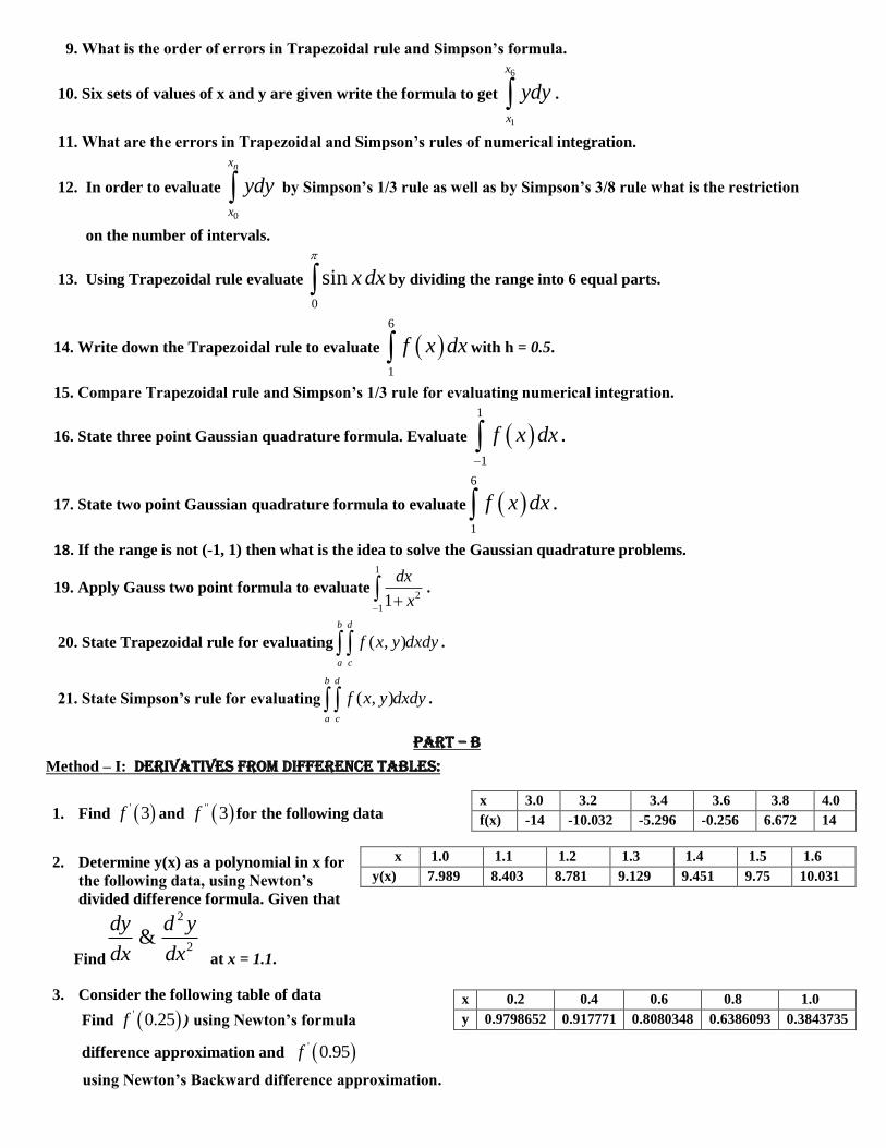
9. What is the order of errors in Trapezoidal rule and Simpson’s formula.

10. Six sets of values of x and y are given write the formula to get

6

1

x

x

ydy .

11. What are the errors in Trapezoidal and Simpson’s rules of numerical integration.

12. In order to evaluate

0

nx

x

ydy by Simpson’s 1/3 rule as well as by Simpson’s 3/8 rule what is the restriction

on the number of intervals.

13. Using Trapezoidal rule evaluate

0

sin x dx

by dividing the range into 6 equal parts.

14. Write down the Trapezoidal rule to evaluate 6

1

f x dx with h = 0.5.

15. Compare Trapezoidal rule and Simpson’s 1/3 rule for evaluating numerical integration.

16. State three point Gaussian quadrature formula. Evaluate 1

1

f x dx

.

17. State two point Gaussian quadrature formula to evaluate 6

1

f x dx .

18. If the range is not (-1, 1) then what is the idea to solve the Gaussian quadrature problems.

19. Apply Gauss two point formula to evaluate

1

2

11

dx

x

.

20. State Trapezoidal rule for evaluating ( , )

b d

a c

f x y dxdy .

21. State Simpson’s rule for evaluating ( , )

b d

a c

f x y dxdy .

PART – B

Method – I: DERIVATIVES FROM DIFFERENCE TABLES:

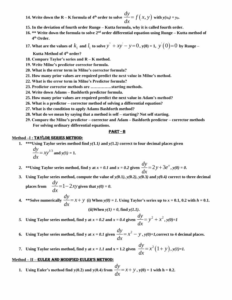
1. Find ' 3f and '' 3f for the following data

2. Determine y(x) as a polynomial in x for

the following data, using Newton’s

divided difference formula. Given that

Find

2

2&

dy d y

dx dx at x = 1.1.

3. Consider the following table of data

Find ' 0.25f ) using Newton’s formula

difference approximation and ' 0.95f

using Newton’s Backward difference approximation.

x 3.0 3.2 3.4 3.6 3.8 4.0

f(x) -14 -10.032 -5.296 -0.256 6.672 14

x 1.0 1.1 1.2 1.3 1.4 1.5 1.6

y(x) 7.989 8.403 8.781 9.129 9.451 9.75 10.031

x 0.2 0.4 0.6 0.8 1.0

y 0.9798652 0.917771 0.8080348 0.6386093 0.3843735

4. The following data gives the velocity of a particle for 20 seconds at an interval of 5 seconds. Find

the initial acceleration using the entire data

5. Find the maximum and minimum value of y tabulated below

6. Give the following data, find ' 6y , ' 5y and the maximum value

7. Find the first two derivatives

of 1

3x at x = 50 and x = 56,

for the given table:

8. Find 'y and

''y at x = 1.25 for the data given

x 1.00 1.05 1.10 1.15 1.20 1.25 1.30

y 1.00000 1.02470 1.04881 1.07238 1.09544 1.11803 1.14017

9. Compute ' 0f and '' 4f from the data

10. Find at x = 1.5 and x = 4.0 from the following data using Newton’s formulae for differentiation.

Method – II : tRapezoidaL aNd simpsoN’s 1/3 aNd 3/8 RuLes:

1. Using Trapezoidal rule, evaluate

1

2

11

dx

x

taking 8 intervals.

2. Evaluate

5

04 5

dx

x by Simpson’s one – third rule and hence find the value of log 5e (n = 10).

3. By dividing the range into ten equal parts, evaluate

0

sin x dx

by Trapezoidal and Simpson’s rule.

Verify your answer with integration

4. Using Simpson’s 1/3 rule evaluate

1

0

xxe dx taking 4 intervals. Compare your result with actual value.

5.

6

2

01

dx

x by (i) Trapezoidal rule (ii) Simpson’s rule. Also check up the results by actual integration.

6. Compute the value of

1.4

0.2

(sin log )x

ex x e dx taking h = 0.2 and using Trapezoidal rule,

Simpson’s 1/3rd rule. Also compare with exact result.

Time(sec) 0 5 10 15 20

Velocity(m/sec) 0 8 14 69 228

x -2 -1 0 1 2 3 4

y 2 -0.25 0 -0.25 2 15.75 56 x 0 52 3 4 7 9

y 4 26 58 112 466 922

x 50 51 52 53 54 55 56

y = 1

3x 3.6840 3.7084 3.7325 3.7563 3.7798 3.8030 3.8259

x 0 1 2 3 4

y 1 2.718 7.381 20.086 54.598

x 1.5 2.0 2.5 3.0 3.5 4.0

y 3.375 7.0 13.625 24.0 38.875 59.0

7. By dividing the range into six equal parts, evaluate

5.2

4

loge xdx using Simpson’s rule.

8. Evaluate

1

2

01

dx

x using Trapezoidal rule with 10 subintervals. Hence approximate the value of π.

9. The velocity of a particle at a distance S from a point on

its path is given by the table below. Estimate the time

taken to travel 60 meters by using Simpson’s one – third

rule. Compare your answer with Simpson’s 3/8 rule and also

using Trapezoidal rule.

10. Dividing the range into 10 equal parts, find the value of

/2

0

sin x dx

by (i) Trapezoidal rule

(ii) Simpson’s 1/3rd rule and (iii)* Simpson’s 3/8 rule(equal part is not mention).

Method – III : RombeRg’s method:

1. Evaluate

2

2

04

dx

x using Romberg’s method. Hence obtain an approximate value for π.

2. Evaluate

1

01

dx

x correct to 3 – decimal places using Romberg’s method. Hence find the value of log 2.e

3. Compute

1

2

01

dx

x by using Trapezoidal rule, taking h = 0.5 and h = 0.25. hence find one value of the above

integration by Romberg’s method.

Method – IV: Gaussian quadrature formulas:

1. Using three – point Gaussian quadrature formulas, evaluate (i)

1

2

11

dx

x

(ii) 1

2

01

dx

t .

2. Evaluate

2 2

4

0

2 1

1 ( 1)

x xdx

x

by Gaussian three point formula.

3. Evaluate

1 2

4

11

x dx

x

by using three points Gauss quadratic.

4. Using three point Gaussian quadrature, evaluate

1

40 1

dx

x .

5. Evaluate

2

2

1

1

1dx

xusing Gauss three point formula.

6. Using Gaussian Two and Three formula, evaluate

3

2

1

1dx

x.

Method – V : doubLe iNtegRaLs usiNg tRapezoidaL aNd simpsoN’s RuLe:

1. Evaluate

2 2

0 0

( , )f x y dxdy by Trapezoidal rule for the following data:

S in meter 0 10 20 30 40 50 60

V m/sec 47 58 64 65 61 52 38

Y x 0 0.5 1 1.5 2

0 2 3 4 5 5

1 3 4 6 9 11

2 4 6 8 11 14

2. Using Simpson’s 1/3 rule evaluate

1 1

0 01

dxdy

x y taking h = k = 0.5.

3. Evaluate

1 2

2 2

0 1

2

(1 )(1 )

xydxdy

x y by Trapezoidal rule with h = k =0.25.

4. Using Trapezoidal rule evaluate

2.0 1.5

1.4 1.0

( 2 )nI x y dxdy . Choosing Δx = 0.15 and Δy = 0.25.

5. Evaluate

1 1

0 0

x ye dxdy

using Simpson’s and Trapezoidal rule.

6. Evaluate

1.4 2.4

1 2

1dxdy

xy by Simpson’s rule taking h = 0.1 and k = 0.1. verify your result by actual integration.

7. Evaluate

5 4

1 1

1dxdy

x y by Trapezoidal rule in x – direction with h = 1 and Simpson’s 1/3 rule in y – direction

with k = 1.

8. Evaluate

2.4 4.4

2 4

xydxdy using Simpson’s rule (h = k = 0.1).

9. *Evaluate

2 1

0 0

4xydxdy by using Simpson’s rule taking h = ¼ and k = ½.

UNIT – IV

INITIAL VALUE PROBLEMS FOR ORDINARY DIFFERENTIAL EQUATIONS

PART – A 1. Write the Taylor’s series formula at y(x0) = y0.

2. Write the merits and demerits of the Taylor method of solution.

3. Which is better Taylor’s method or R-K method?

4. Solve the differential equation , 0 1dy

x y xy ydx

by Taylor series method to get the value

of y at x = h.

5. What is meant by initial value problem and give an example for it.

6. Find y(0.1) by Taylor’s series given 1 , (0) 1dy

y ydx

.

7. Write down the fourth order Taylor Algorithm.

8. State Modified Euler algorithm to solve ' ,y f x y , y(x0) = y0, at x = x0 + h.

9. Write down Euler algorithm to the differential equation ,dy

f x ydx

.

10. Find y(0.2) when ' 22y xy , y(0) = 1 and h = 0.2 by Euler’s method.

11. Solve 1dy

ydx

, y(0) = 0, for x = 0.1 by Euler’s method.

12. Solve , 0 1dy

y ydx

to find y(0.01) using Euler method.

13. Write the Runge – Kutta algorithm of second order for solving ' ,y f x y , y(x0) = y0.

14. Write down the R – K formula of 4th order to solve ,dy

f x ydx

with y(x0) = y0.

15. In the deviation of fourth order Runge – Kutta formula, why it is called fourth order.

16. ** Write down the formula to solve 2nd order differential equation using Runge – Kutta method of

4th Order.

17. What are the values of 1k and

1l to solve" ' 0y xy y , y(0) = 1, ' 0 0y by Runge –

Kutta Method of 4th order?

18. Compare Taylor’s series and R – K method.

19. Write Milne’s predictor corrector formula.

20. What is the error term in Milne’s corrector formula?

21. How many prior values are required predict the next value in Milne’s method.

22. What is the error term in Milne’s Predictor formula?

23. Predictor corrector methods are ……………starting methods.

24. Write down Adams – Bashforth predictor formula.

25. How many prior values are required predict the next value in Adam’s method?

26. What is a predictor – corrector method of solving a differential equation?

27. What is the condition to apply Adams Bashforth method?

28. What do we mean by saying that a method is self – starting? Not self starting.

29. Compare the Milne’s predictor – corrector and Adam – Bashforth predictor – corrector methods

For solving ordinary differential equations.

PART - B

Method –I : Taylor series method: 1. ***Using Taylor series method find y(1.1) and y(1.2) correct to four decimal places given

1/3dy

xydx

and y(1) = 1.

2. **Using Taylor series method, find y at x = 0.1 and x = 0.2 given 2 3 xdyy e

dx , y(0) = 0.

3. Using Taylor series method, compute the value of y(0.1), y(0.2), y(0.3) and y(0.4) correct to three decimal

places from 1 2dy

xydx

given that y(0) = 0.

4. **Solve numerically dy

x ydx

(i) When y(0) = 1. Using Taylor’s series up to x = 0.1, 0.2 with h = 0.1.

(ii)When y(1) = 0, find y(1.1).

5. Using Taylor series method, find y at x = 0.2 and x = 0.4 given 2 2dy

y xdx

, y(0)=1

6. Using Taylor series method, find y at x = 0.1 given 2dy

x ydx

, y(0)=1,correct to 4 decimal places.

7. Using Taylor series method, find y at x = 1.1 and x = 1.2 given 2 1dy

x ydx

, y(1)=1.

Method – II – euLeR aNd modified euLeR’s method:

1. Using Euler’s method find y(0.2) and y(0.4) from dy

x ydx

, y(0) = 1 with h = 0.2.

2. Using modified Euler’s method, solve 1dy

ydx

, y(0) = 0, for x = 0.1, 0.2, and 0.3. compare your results with

exact solutions.

3. Using modified Euler’s method find y at x = 0.1 and x = 0.2 given 2

, (0) 1dy x

y ydx y

.

4. Solve 10log , (0) 2dy

x y ydx

by Euler’s Modified method and find the values of y(0.2), y(0.4),and

y(0.6) take h = 0.2.

5. Using Modified Euler method find

a. y(0.1) and y(0.2) given ' 2 2y x y , y(0) = 1 with h = 0.1

b. y(0.2) and y(0.4) given ' 2 2y x y , y(0) = 1 with h = 0.2.

6. Find y(0.25) and y(0.5), using Modified Euler’s Method with h = 0.25 given that' 23y x y ,

y(0) = 4. Compare the values with the exact solutions.

7. **consider the initial value problem 2 1, 0 0.5dy

y x ydx

using the modified Euler method,

find y(0.2)

8. *Using modified Euler’s method, find y(4.1) and y(4.2) if 25 2 0, 4 1dy

x y ydx

.

Method – III: 4th order R – K method:

1. Find y(0.2) using R – K method of order 4 from 'y x y , y(0) = 1.

2. Given 2dy

x y xdx

, y(0) = 1, using R – K method of 4th order find y at x = 0.1.

3. Compute y(0.2) given

2 2

2 2

dy y x

dx y x

, y(0) = 1 by R – K method.

4. Find y(0.8) given that ' 2y y x , y(0.6) = 1.7379 by using R – K method of order 4 with h = 0.1

5. Using R.K. method of 4th order find y(0.1) given initial value problem2dy

x ydx

, y(0) = 1.

6. Find y(0.2) and y(0.4) using R – K method of order 4 from ' 3y x y , y(0) = 2.

7. Find y(0.1) using R – K method of order 4 from 1dy

dx x y

, y(0) = 1.

8. Find y(0.2), given logdy

x ydx

, y(0) = 1 using R – K method of 4th order, taking h = 0.1.

Method – IV : 2ND ORDER DIFFERENTIAL EQUATION USING R – K METHOD OF 4TH ORDER:

1. **Using R – K method of order 4, solve " 22 ' 2 sinxy y y e x with y(0) = -0.4 ' 0 0.6y .

2. Use R – K 4th order method to find y(0.2) for the equation" ' 0y xy y given that y(0) = 1,

' 0 0, 0.2y takeh

3. **Given " ' 0y xy y , y(0) = 1, ' 0 0y . Find the value of y(0.1) by R – K method of 4th order.

Method – V : miLNe’s pRedictoR aNd coRRectoR method:

1. * Using Milne’s method find y(2) if y(x) is the solution of 2

dy x y

dx

given y(0) = 2, y(0.5) = 2.636,

y(1) = 3.8595 and y(1.5) = 4.968.

2. Using Milne’s method , find y (4.4) given ' 22 2 0xy y , y(4) = 1, y(4.1) = 1.0049,

y(4.2) = 1.0097 and y(4.3) = 1.0143.

3. ***Solve 2 , (0) 1

dyxy y y

dx , using Milne’s predictor – corrector formula and find y(0.4).

Using Taylor series method to find y(0,.1), y(0.2) and y(0.3).

4. Solve

2 , (0) 1dy

y x ydx

(i) Find y(0.1) and y(0.2) by R – K method of order 4.

(ii) Find y(0.3) by Euler’s method

(iii) Find y(0.4) by Milne’s predictor – corrector method.

5. Solve 2 2 2

dyx y

dx , using Milne’s predictor – corrector method for x = 0.3,y(0) = 1. Evaluate

the values of y for x = - 0.1, 0.1 and 0.2 using Taylor’s series.

6. **Using Milne’s method find y(4.4) given' 25 2 0xy y given y(4) = 1, y(4.1)= 1.0049,

y(4.2) = 1.0097 and y(4.3) = 1.0143.

7. Given 2 21

2

y xdy

dx

and y(0) = 1, y(0.1) = 1.06, y(0.2) = 1.12, y(0.3) = 1.21, evaluate y(0.4) by

Milne’s predictor – corrector method.

8. *Given that 21

dyy

dx

; y(0.6)= 0.6841, y(0.4) = 0.4228, y(0.2) = 0.2027, y(0) = 0, find y(-0.2) using Milne’s

method.

Method – VI – adam’s pRedictoR aNd coRRectoR methods:

1. Given 2 1dy

x ydx

, y(1) = 1, y(1.1) = 1.233, y(1.2) = 1.548, y(1.3) = 1.979, evaluate y(1.4) by Adams –

Bashforth method.

2. Solve 1dy

ydx

with the initial condition x = 0, y = 0, using Euler’s algorithm and tabulate the solutions at x

= 0.1, 0.2, 0.3, 0.4. using these remits find y(0.5) using Adams – Bashforth predictor – corrector method.

3. Using Adams – Bashforth predictor – corrector formulae, evaluate y(1.4). if y satisfies2

1dy y

dx x x and y(1)

= 1, y(1.1) = 0.996, y(1.2) = 0.986, y(1.3) = 0.972.

4. Find y(0.1), y(0.2,), y(0.3), from' 2y x y ,y(0) = 1 using Taylor’s series method and hence obtain y(0.4)

using Adams – Bashforth method.

5. By using Adam’s pc method find y when x = 0.4, given 2

dy xy

dx , y(0) = 1, y(0.1) = 1.01, y(0.2) = 1.022, y(0.3)

= 1.023.

Method – VII - Simultaneous differential equations:

1. Solve for y(0.1) from the simultaneous differential equations 2dy

y zdx

; 3dz

y zdx

; y(0) = 0, z(0) =

0.5 using Runge kutta method of the fourth order.

UNIT – V

BOUNDARY VALUE PROBLEMS IN ORDINARY

AND PARTIAL DIFFERENTIAL EQUATIONS

PART – A 1. Write an explicit formula to solve numerically the heat equation(parabolic equation) uxx – aut = 0.

2. Write down the Crank – Nicolson formula to solve ut = uxx.

3. Write down the implicit formula to solve one dimensional heat flow equation

4. What is the central difference approximation for "y

5. Write the difference scheme for solving the Poisson equation 2 ( , )u f x y .

6. Write down the finite difference formula for 'y and "y .state the finite difference scheme to solve the

equation 2

tt xxy a y .

7. Classify the PDE 0xx yyy xu .

8. Write down Bender – Schmidt’s difference scheme in general form and using suitable value of , write the

scheme in simplified form.

9. State Standard Five Point Formula with relevant diagram.

10. Define a difference quotient.

11. State the SFPF in solving Laplace equation.

12. State the implicit scheme to solve the dimensional heat equation numerically.

13. Write the difference scheme quotients of uxx and uyy.

14. Write the finite difference scheme for the second order differential equation "y f ,1

hn

.

15. State the explicit finite difference scheme for one dimensional wave equation

2 22

2 2

u u

t x

.

16. Define SFPF and DFPF.

17. Define elliptic, parabolic and hyperbolic type of partial differential equations.

PART – B

METHOD – I – BENDER SCHMIDT METHOD:

1. Solve

2

2

u u

x t

, subject to u(0, t) = u(1, t) = 0 and u(x, 0) = sinπx, 0 < x < 1 using Bender – Schmidt method.

2. Solve with the conditions u(0, t) = 0 = u(4, t), u(x, 0) = x(4 - x)

(1) Taking h = 1 employing Bender- Schmidt recurrence equation. Continue the solution through 10 time

steps

(2) Assume h = 1. Find the values of up to t = 5, using explicit method.

3. Solve with boundary conditions u(0, t) = 0, u(8, t) = 0, u(x, 0) = x(8 - x)/2up to t = ½ , taking h = 1, k = 1/8.

4. Given

2

20

f f

x t

, f(0, t) = f(5, t) = 0, f(x, 0) = x2(25 – x2), find f in the range taking h = 1 and upto 5

seconds.

Method – II:

1. Find the pivotal values of the equation

2 2

2 24

u u

t x

with given conditions u(0, t) = 0, u(4, t) = 0,

u(x, 0) = x(4 - x) and ( ,0)

0u x

t

by taking h = 1, for 4 time steps.

2. Evaluate the Pivotal values of the equation taking h = 1 and up to on half of the period of the oscillation 16uxx

– utt = 0 given u(0, t) = u(5, t) = ut(x, 0) = 0and u(x, 0) = x2(5 - x).

3. Solve 25uxx – utt = 0 for u at the Pivotal points given u(0, t) = u(5, t) = ut(x, 0) = 0 and u(x, 0) = 2x for 0

< x < 2.5 and = 10 – 2x for 2.5 < x <5 for one half period of vibrations.

4. Solve the equation

2 2

2 2

u u

x t

, 0 < x < 1, t > 0 satisfying the conditions u(x, 0) = 0, u(0, t) = 0 and u(1, t) =

½sinπt. Compute u(x, t) for 4 time – steps by taking h = ¼.

Method – III:

1. Solve the equation "y x y with the boundary conditions y(0) = y(1) = 0.

2. Solve the finite difference method, the boundary value problem "( ) ( ) 0y x y x , where y(0) = 0 and y(1)

= 1, taking h = 0.25.

3. Using the finite difference method, compute y(0.5), given " 64 10 0y y , x ∈ (0, 1), y(0) = y(1) = 0, sub

dividing the interval into (1) 4 equal parts (2) 2 equal parts.

4. Solve " 0y y with the boundary conditions y(0) = 0 and y(1) = 1.

Method – IV: 1. Solve the elliptic equation for the following square mesh with boundary values as shown

0 500 1000 500 0

1000 1000

2000 2000

1000 1000

0 500 1000 500 0

2. Solve 2 2 28u x y for square mesh given u = 0 on the boundaries dividing the square in to 16 sub squares

of length 1 unit.

3. *Solve uxx +uyy = -10(x2 +y2 + 10) over the square mesh with sides x = 0, y = 0, x = 3, y = 3 with u = 0, on the

boundary and mesh length 1 unit.

4. Solve 2 0u over the square mesh of side 4 units, satisfying the boundary conditions.

(a) u(0, y) = 0 for 0 < y < 4

(b) u(4, y) = 12 +y for 0 < y < 4

(c) u(x, 0) = 3x for 0 < x < 4

(d) u(x, 4) = x2 for 0 < x < 4.

5. Solve uxx +uyy = 0 in 0 ≤ x ≤ 4, 0 ≤ y ≤ 4. Given that u(0, y) = 0, u(4, y) = 8 + 2y; u(x, 0) = x2/2 and u(x, 4) = 2

taking h = k = 1. Obtain the result correct to one decimal.

6. Solve2 0u in the square region bounded by x = 0, x= 4, y = 0, y = 4 and with boundary conditions u(0, y)

= y2/2, u(4, y) = y2, u(x, 0) = 0and u(x, 4) = 8 +2x taking h = k = 1. (Perform 4 iterations)