XIX Ciclo - Semantic Scholar · Galli, Felipe Navarro, Victor Vera Valdes and Andrea Tramontani....
140
UNIVERSIT ` A DEGLI STUDI DI BOLOGNA Dottorato di Ricerca in Automatica e Ricerca Operativa MAT/09 XIX Ciclo The Vertex Coloring Problem and its Generalizations Enrico Malaguti Il Coordinatore Il Tutor Prof. Claudio Melchiorri Prof. Paolo Toth A.A. 2003–2006
-
Upload
nguyentuyen -
Category
Documents
-
view
213 -
download
0
Transcript of XIX Ciclo - Semantic Scholar · Galli, Felipe Navarro, Victor Vera Valdes and Andrea Tramontani....

UNIVERSITA DEGLI STUDI DI BOLOGNA
Dottorato di Ricerca inAutomatica e Ricerca Operativa
MAT/09
XIX Ciclo
The Vertex Coloring Problem
and its Generalizations
Enrico Malaguti
Il Coordinatore Il TutorProf. Claudio Melchiorri Prof. Paolo Toth
A.A. 2003–2006

Contents
Acknowledgments v
Keywords vii
List of figures ix
List of tables xi
1 Introduction 11.1 The Vertex Coloring Problem and its Generalizations . . . . . . . . . . . . . . 11.2 Fair Routing . . . . . . . . . . . . . . . . . . . . . . . . . . . . . . . . . . . . 6
I Vertex Coloring Problems 9
2 A Metaheuristic Approach for the Vertex Coloring Problem 112.1 Introduction . . . . . . . . . . . . . . . . . . . . . . . . . . . . . . . . . . . . . 11
2.1.1 The Heuristic Algorithm MMT . . . . . . . . . . . . . . . . . . . . . . 122.1.2 Initialization Step . . . . . . . . . . . . . . . . . . . . . . . . . . . . . 13
2.2 PHASE 1: Evolutionary Algorithm . . . . . . . . . . . . . . . . . . . . . . . . 152.2.1 Tabu Search Algorithm . . . . . . . . . . . . . . . . . . . . . . . . . . 152.2.2 Evolutionary Diversification . . . . . . . . . . . . . . . . . . . . . . . . 182.2.3 Evolutionary Algorithm as part of the Overall Algorithm . . . . . . . 21
2.3 PHASE 2: Set Covering Formulation . . . . . . . . . . . . . . . . . . . . . . . 222.3.1 The General Structure of the Algorithm . . . . . . . . . . . . . . . . . 24
2.4 Computational Analysis . . . . . . . . . . . . . . . . . . . . . . . . . . . . . . 252.4.1 Performance of the Tabu Search Algorithm . . . . . . . . . . . . . . . 252.4.2 Performance of the Evolutionary Algorithm . . . . . . . . . . . . . . . 262.4.3 Performance of the Overall Algorithm . . . . . . . . . . . . . . . . . . 262.4.4 Comparison with the most effective heuristic algorithms . . . . . . . . 30
2.5 Conclusions . . . . . . . . . . . . . . . . . . . . . . . . . . . . . . . . . . . . . 33
3 An Evolutionary Approach for Bandwidth Multicoloring Problems 373.1 Introduction . . . . . . . . . . . . . . . . . . . . . . . . . . . . . . . . . . . . . 373.2 An ILP Model for the Bandwidth Coloring Problem . . . . . . . . . . . . . . 393.3 Constructive Heuristics . . . . . . . . . . . . . . . . . . . . . . . . . . . . . . 403.4 Tabu Search Algorithm . . . . . . . . . . . . . . . . . . . . . . . . . . . . . . 40
i

ii CONTENTS
3.5 The Evolutionary Algorithm . . . . . . . . . . . . . . . . . . . . . . . . . . . . 433.5.1 Pool Management . . . . . . . . . . . . . . . . . . . . . . . . . . . . . 44
3.6 Computational Analysis . . . . . . . . . . . . . . . . . . . . . . . . . . . . . . 473.6.1 Performance of the Tabu Search Algorithm . . . . . . . . . . . . . . . 473.6.2 Performance of the Evolutionary Algorithm . . . . . . . . . . . . . . . 51
3.7 Conclusions . . . . . . . . . . . . . . . . . . . . . . . . . . . . . . . . . . . . . 53
4 Models and Algorithms for a Weighted Vertex Coloring Problem 574.1 Introduction . . . . . . . . . . . . . . . . . . . . . . . . . . . . . . . . . . . . . 574.2 ILP models . . . . . . . . . . . . . . . . . . . . . . . . . . . . . . . . . . . . . 59
4.2.1 Model M1 . . . . . . . . . . . . . . . . . . . . . . . . . . . . . . . . . . 594.2.2 Model M2 . . . . . . . . . . . . . . . . . . . . . . . . . . . . . . . . . . 594.2.3 Comparing Models M1 and M2 . . . . . . . . . . . . . . . . . . . . . . 604.2.4 Model M3 . . . . . . . . . . . . . . . . . . . . . . . . . . . . . . . . . . 62
4.3 The 2-phase Heuristic Algorithm . . . . . . . . . . . . . . . . . . . . . . . . . 634.3.1 Constructive heuristics . . . . . . . . . . . . . . . . . . . . . . . . . . . 654.3.2 Column Optimization . . . . . . . . . . . . . . . . . . . . . . . . . . . 66
4.4 Post-optimization procedures . . . . . . . . . . . . . . . . . . . . . . . . . . . 664.4.1 An ILP model for matrix post-optimization . . . . . . . . . . . . . . . 674.4.2 An Assignment based procedure for matrix post-optimization . . . . . 69
4.5 Computational Analysis . . . . . . . . . . . . . . . . . . . . . . . . . . . . . . 704.5.1 Weighted Vertex Coloring Instances . . . . . . . . . . . . . . . . . . . 704.5.2 Traffic Decomposition Matrix Instances . . . . . . . . . . . . . . . . . 74
4.6 Conclusions . . . . . . . . . . . . . . . . . . . . . . . . . . . . . . . . . . . . . 76
5 Lower and Upper Bounds for the Bounded Vertex Coloring Problem 775.1 Introduction . . . . . . . . . . . . . . . . . . . . . . . . . . . . . . . . . . . . . 775.2 ILP model . . . . . . . . . . . . . . . . . . . . . . . . . . . . . . . . . . . . . . 785.3 Lower Bounds . . . . . . . . . . . . . . . . . . . . . . . . . . . . . . . . . . . . 79
5.3.1 A surrogate relaxation . . . . . . . . . . . . . . . . . . . . . . . . . . . 805.3.2 A Lower Bound based on Matching . . . . . . . . . . . . . . . . . . . . 81
5.4 Upper Bounds . . . . . . . . . . . . . . . . . . . . . . . . . . . . . . . . . . . 825.4.1 Evolutionary Algorithm . . . . . . . . . . . . . . . . . . . . . . . . . . 83
5.5 Computational Experiments . . . . . . . . . . . . . . . . . . . . . . . . . . . . 865.6 Conclusions . . . . . . . . . . . . . . . . . . . . . . . . . . . . . . . . . . . . . 86
II Fair Routing 93
6 On the Fairness of ad-hoc Telecommunication Networks 956.1 Introduction . . . . . . . . . . . . . . . . . . . . . . . . . . . . . . . . . . . . . 956.2 A Model for Fair Routing . . . . . . . . . . . . . . . . . . . . . . . . . . . . . 97
6.2.1 Preliminaries . . . . . . . . . . . . . . . . . . . . . . . . . . . . . . . . 976.2.2 A Proposed Model . . . . . . . . . . . . . . . . . . . . . . . . . . . . . 986.2.3 Formulation . . . . . . . . . . . . . . . . . . . . . . . . . . . . . . . . . 101
6.3 Computational Experiments . . . . . . . . . . . . . . . . . . . . . . . . . . . . 1026.3.1 Computational Experiments with the First Fairness Measure . . . . . 103

CONTENTS iii
6.3.2 Computational Experiments with the Second Fairness Measure . . . . 1046.3.3 Access Point Configuration . . . . . . . . . . . . . . . . . . . . . . . . 106
6.4 A Distributed Routing Algorithm . . . . . . . . . . . . . . . . . . . . . . . . . 1096.4.1 Experimental Results . . . . . . . . . . . . . . . . . . . . . . . . . . . 112
6.5 Conclusions . . . . . . . . . . . . . . . . . . . . . . . . . . . . . . . . . . . . . 114
Bibliography 115

iv CONTENTS

Acknowledgments
Many thanks go to the advisor of this thesis, Paolo Toth, and to all the friends that co-authored the work presented in this pages: Paolo Toth and Michele Monaci, Andrea Lodi,Nicolas Stier-Moses, Alessandra Giovanardi, Albert Einstein Fernandez Muritiba, ManuelIori.
Thanks are also due to other components of the Operations Research group in Bologna,for their help and friendly support: Silvano Martello, Daniele Vigo, Alberto Caprara, toValentina Cacchiani and Matteo Fortini, and to Ph.D. students Claudia D’Ambrosio, LauraGalli, Felipe Navarro, Victor Vera Valdes and Andrea Tramontani.
I want to thank my family too, for supporting me in all my decisions, and all my friends,some of those have been tolerating me for almost 30 years.
Finally, a thank goes to Francesca, who is a very special person.
Bologna, March 12, 2004
Enrico Malaguti
v

vi ACKNOWLEDGMENTS

Keywords
Vertex Coloring, Graph, Mathematical Models, Heuristic Algorithms,Evolutionary Algorithms, Ad Hoc Networks, Fairness.
vii

viii Keyworks

List of Figures
4.1 Simple graph for which the LP relaxations of M1 and M2 have different values. 62
6.1 An example with fairness 1/2. . . . . . . . . . . . . . . . . . . . . . . . . . . . 1006.2 Total energy consumption (log) and fairness. First definition of fairness. . . . 1036.3 Flow distribution for minimal fairness of 0, 0.025, 0.5, 0.1, 0.3, 0.5, 0.8, 0.9,
1.0. First definition of fairness. . . . . . . . . . . . . . . . . . . . . . . . . . . 1056.4 Total energy consumption and fairness. Comparison between first and second
definition of fairness. . . . . . . . . . . . . . . . . . . . . . . . . . . . . . . . . 1066.5 Flow distribution for minimal fairness of 0.1, 0.3, 0.5, 0.8 and 1.0. Second
definition of fairness. . . . . . . . . . . . . . . . . . . . . . . . . . . . . . . . . 1076.6 Energy consumption of the single nodes and fairness, power control. Second
definition of fairness. . . . . . . . . . . . . . . . . . . . . . . . . . . . . . . . . 1086.7 Energy consumption of the single nodes and fairness, no power control. Second
definition of fairness. . . . . . . . . . . . . . . . . . . . . . . . . . . . . . . . . 1096.8 Total energy consumption (log) and fairness. Access point configuration, first
definition of fairness. . . . . . . . . . . . . . . . . . . . . . . . . . . . . . . . . 1106.9 Flow distribution for minimal fairness of 0.0, 0.1, 0.3, 0.5, 0.8 and 1.0. Access
point configuration. . . . . . . . . . . . . . . . . . . . . . . . . . . . . . . . . . 1116.10 Total energy consumption and fairness, power control. Decentralized Algo-
rithm and Benchmark. . . . . . . . . . . . . . . . . . . . . . . . . . . . . . . . 1146.11 Energy consumption of the single nodes and fairness, power control. Decen-
tralized Algorithm. . . . . . . . . . . . . . . . . . . . . . . . . . . . . . . . . . 1156.12 Total energy consumption and fairness, no power control. Decentralized Algo-
rithm and Benchmark. . . . . . . . . . . . . . . . . . . . . . . . . . . . . . . . 1166.13 Energy consumption of the single nodes and fairness, no power control. De-
centralized Algorithm. . . . . . . . . . . . . . . . . . . . . . . . . . . . . . . . 117
ix

x LIST OF FIGURES

List of Tables
2.1 Performance of the Tabu Search Algorithm. . . . . . . . . . . . . . . . . . . . 272.2 Performance of the Evolutionary Algorithm. . . . . . . . . . . . . . . . . . . . 292.3 Parameters of Algorithm MMT. . . . . . . . . . . . . . . . . . . . . . . . . . 302.4 Performance of the Algorithm MMT. . . . . . . . . . . . . . . . . . . . . . . . 312.5 Performance of the most effective heuristics in decision version. . . . . . . . . 342.6 Performance of the most effective heuristics in optimization version. . . . . . 352.7 Average gap on the common subset of instances. . . . . . . . . . . . . . . . . 36
3.1 Tabu Search Algorithm: Bandwidth Coloring Instances. . . . . . . . . . . . . 493.2 Tabu Search Algorithm: Bandwidth Multicoloring Instances. . . . . . . . . . 503.3 Performance of the Evolutionary Algorithm and comparison with the most
effective heuristic algorithms for the Bandwidth Coloring Problem. . . . . . . 543.4 Performance of the Evolutionary Algorithm and comparison with the most
effective heuristic algorithms for the Bandwidth Multicoloring Problem. . . . 55
4.1 Results on instances derived from DIMACS instances. . . . . . . . . . . . . . 734.2 Results on Traffic Decomposition Matrix Instances. . . . . . . . . . . . . . . . 75
5.1 Upper bounds results for classes 1–4. . . . . . . . . . . . . . . . . . . . . . . . 875.2 Upper bounds results for classes 5–8. . . . . . . . . . . . . . . . . . . . . . . . 885.3 Lower bounds results for classes 1–4. . . . . . . . . . . . . . . . . . . . . . . . 895.4 Lower bounds results for classes 5–8. . . . . . . . . . . . . . . . . . . . . . . . 905.5 Comparison between lower and upper bounds. . . . . . . . . . . . . . . . . . . 91
xi

xii LIST OF TABLES

Chapter 1
Introduction
The main topic of this thesis is the Vertex Coloring Problem and its generalizations, for whichmodels, algorithms and bounds are proposed in the First Part.
The Second Part is dedicated to a different problem on graphs, namely a Routing Problemin telecommunication networks where not only the efficiency, but also the fairness of thesolution are considered.
1.1 The Vertex Coloring Problem and its Generalizations
Consider the following problems:
1. Color the map of England, in such a way that no two counties touching with a commonstretch of boundary are given the same color, by using the smallest number of colors 1.
2. Organize the timetable of examinations of a university. Each examination needs a timeslot, and the university wants to organize as many examinations in parallel as possible,without exceeding the availability of classrooms, in order to reduce the number of timeslots. Since students can take more than one course, and they must be able to take partin the exams of all the courses they have followed, two examinations cannot be scheduledat the same time, if there is at least one student taking both the corresponding courses.
3. Radio spectrum has to be assigned to broadcast emitting stations, in such a way thatadjacent stations, which could interfere, use different frequencies (each station may needone or more frequencies). In general it is required that two interfering stations use fre-quencies that are far each other, with a distance depending on propagation phenomena.Since radio spectrum is a very scarce and expensive resource, the allocation of frequencymust be the most efficient, i.e. the total number of frequencies has to be minimized.
4. In the metal industry, metal coils are heated in furnaces. Each coil has to be heated forat least a given amount of time (different for each coil), and coils heated together must
1Four are enough for any map, see Appel, Haken and Koch [10], the Four Color Conjecture was proposedby Francis Guthrie in 1852
1

2 Introduction
be compatible, i.e. they must have similar heights. The problem is to decide which coilswill be heated together, in order to minimize the total heating time.
5. An nXn traffic matrix has to be transmitted through an analogical satellite. Each entryof the matrix represents the amount of traffic (i.e. the connection duration) to be sentfrom a transmitting antenna to a receiving antenna. In order to be transmitted, thematrix must be decomposed into mode matrices, i.e. matrices with at most one nonzero element (corresponding to the traffic sent for each pair of transmitting-receivingantennas) per row and per column, in such a way that the sum of the mode matricescorresponds to the original traffic matrix. The transmitting time of each mode matrixcorresponds to its largest element, and the problem is to minimize the total transmittingtime.
6. Some vehicles are used to deliver items. Some items cannot travel on the same vehicle,because they are dangerous or require special equipment. The problem is to minimizethe number of vehicles, by considering that each item has a weight and the capacity ofvehicles is bounded.
7. Aircrafts are approaching an airport. The traffic control system assigns them an alti-tude, where they wait their landing time. If the arrival intervals of two planes overlap,they cannot use the same altitude. The available altitudes are limited, and they haveto be assigned efficiently.
At first sight, the problems listed above have nothing in common. They consider coloring amap, telecommunications, heating in a furnace, timetabling, delivery, assignment of altitudesto aircrafts, etc. However, they all are optimization problems with a common structure.
A resource is shared among users. Some users can access the resource simultaneously,while others are pairwise incompatible, and the resource must be duplicated. The problemasks how to group the users that will access the resource simultaneously, in such a way thatthe number of copies of the resource is minimized.
Problems with this structure have been represented as Vertex Coloring Problems. For-mally, consider an undirected graph G = (V,E), where V is the set of vertices and E the set ofedges, having cardinality n and m, respectively. The Vertex Coloring Problem (VCP) requiresto assign a color to each vertex in such a way that colors on adjacent vertices are different andthe number of colors used is minimized. Vertex Coloring is a well known NP-hard problem(see Garey and Johnson [53]), and has received a large attention in the literature, not only forits real world applications in many engineering fields, a subset of those is reported above asan example, but also for its theoretical aspects and for its difficulty from the computationalpoint of view. Actually, exact algorithms proposed for VCP are able to solve consistently onlysmall instances, with up to 100 vertices for random graphs. On the other hand, real worldapplications commonly deal with graphs of hundreds or thousands of vertices, for which theuse of heuristic and metaheuristic techniques is necessary.
Since n colors will always suffice for coloring any graph, a straightforward Integer LinearProgramming (ILP) model for VCP can be obtained by defining the following two sets ofbinary variables: variables xih (i ∈ V, h = 1, . . . , n), with xih = 1 iff vertex i is assigned tocolor h, and variables yh (h = 1, . . . , n) denoting if color h is used in the solution. A possiblemodel for VCP reads:

The Vertex Coloring Problem and its Generalizations 3
minn∑
h=1
yh(1.1)
n∑
h=1
xih = 1 ∀i ∈ V(1.2)
xih + xjh ≤ yh ∀(i, j) ∈ E, h = 1, . . . , n(1.3)xih ∈ {0, 1} ∀i ∈ V, h = 1, . . . , n(1.4)yh ∈ {0, 1} h = 1, . . . , n(1.5)
Objective function (1.1) minimizes the number of colors used. Constraints (1.2) requirethat each vertex is colored, while (1.3) impose that at most one of a pair of adjacent verticesreceive a color, when the color is used. Finally, (1.5) and (1.4) impose the integrality of thevariables. Albeit more sophisticated models can lead to better computational results whensolved by means of exact or heuristic techniques, and are discussed in the following of thisthesis, the model using binary variables xih and yh has the advantage of the clarity, and canbe easily extended to VCP generalizations, as discussed in the following.
From the list of proposed problems, Problem 1 is a classical VCP, by defining a vertex foreach county of England, and an edge connecting two vertices if the corresponding countiesare touching with a common stretch of boundary. Problem 7 is a VCP too, if we associatea vertex to each aircraft and an edge connecting two vertices if the arrival intervals of thecorresponding aircrafts overlap.
In many practical situation, the number of users that can access to a resource is bounded,or it may happen that each user consumes a (possibly different) fraction of the resource, andthe total capacity of the resource is limited. We can model this situation by assigning apositive weight wi to each vertex, and imposing a capacity constraint on the total weight ofthe vertices that receive the same color. The corresponding problem is known as BoundedVertex Coloring Problem (BVCP) or Bin Packing Problem with Conflicts (where the BinPacking Problem requires to assign a set of items, each one with a positive weight, to thesmallest number of bins, each bin with the same capacity C, see Martello and Toth [88]). IfC is the capacity of each color, we can impose a capacity constraint as follows:
n∑
i=1
wixih ≤ C ∀h = 1, . . . , n(1.6)
Model (1.1)–(1.4), with constraint (1.6) is a BVCP. When all the weights of the verticesare equal to 1, constraint (1.6) determines the maximum number of vertices which can receivethe same color. This models for example Problem 2, if a vertex i of weight 1 is associatedto each examination, and a color h corresponds to a time slot: vertex i is assigned color hiff examination i is scheduled in time slot h; two vertices are adjacent if the correspondingexaminations cannot be scheduled in the same time slot, because there is at least one studentwho may want to take part in both the examinations. Each time slot has a maximum capacityC, corresponding to the number of classrooms available for the examinations. Problem 6 canbe modelled as a BVCP as well, if a vertex is associated to each item, a color to each vehicle,and C represents the capacity of a vehicle with respect to a given dimension.

4 Introduction
In the Bandwidth Coloring Problem (BCP) distance constraints are imposed betweenadjacent vertices, replacing the difference constraints (1.3) of model (1.1)–(1.4), and thelargest color used is minimized. A distance d(i, j) is defined for each edge (i, j) ∈ E, and theabsolute value of the difference between the colors assigned to i and j must be at least equalto this distance: |c(i)− c(j)| ≥ d(i, j) (in this problem more than n colors may be necessary,so let H be the set of available colors).
A possible model for BCP, using binary variables xih and yh defined above, and a contin-uous variable k, reads:
min k(1.7)k ≥ yhh h ∈ H(1.8) ∑
h∈H
xih = 1 i ∈ V(1.9)
xih + xjl ≤ 1 (i, j) ∈ E, h ∈ H, l ∈ {h− d(i, j) + 1, ..., h + d(i, j)− 1}(1.10)xih ≤ yh i ∈ V, h ∈ H(1.11)
xi,h ∈ {0, 1} i ∈ V, h ∈ H(1.12)yh ∈ {0, 1} h ∈ H(1.13)
The objective function (1.7) (in conjunction with constraints (1.8)) asks for minimizingthe maximum color used. Note that in BCP the number of colors assigned to the verticescan be smaller than maximum color used. Constraints (1.10) state that the absolute value ofthe difference between the colors assigned to vertices i and j must be at least equal to d(i, j).Constraints (1.11) ensure that if a vertex i uses a color h, then color h results as used.
In the Multicoloring Problem (MCP) a positive request ri is defined for each vertex i ∈ V ,representing the number of colors that must be assigned to vertex i, so that for each (i, j) ∈ Ethe intersection of the color sets assigned to vertices i and j is empty. The BandwidthMulticoloring Problem (BMCP) is the combination of the two problems above. Each vertex imust be assigned ri colors, and each of these colors must respect the distance d(i, j) with allthe colors assigned to any adjacent vertex j. In this case, loop d(i, i) represents the minimumdistance between different colors assigned to the same vertex i. The three problems definedabove, and in particular the BMCP (which generalizes the BCP and MCP) received a wideinterest in telecommunications [4], where they model frequency assignment problems, like theone proposed in Problem 3
In all the problems and corresponding models considered up to now, the cost of each colorhas been set equal to one. In this thesis we consider also a Weighted version of the VertexColoring Problem (WVCP) in which each vertex i of a graph G has associated a positiveweight wi, and the objective is to minimize the sum of the costs of the colors used, where thecost of each color is given by the maximum weight of the vertices assigned to that color. Themost natural model for this problem requires, in addition to the binary xih variables, sayingif vertex i receives color h, continuous variables zh (h = 1, . . . , n), denoting the cost of colorh in the solution. The corresponding model for WVCP is:
minn∑
h=1
zh(1.14)

The Vertex Coloring Problem and its Generalizations 5
zh ≥ wi xih i ∈ V, h = 1, . . . , n(1.15)n∑
h=1
xih = 1 i ∈ V(1.16)
xih + xjh ≤ 1 (i, j) ∈ E, h = 1, . . . , n(1.17)xih ∈ {0, 1} i ∈ V, h = 1, . . . , n(1.18)
where objective function (1.14) minimizes the sum of the costs of the colors, which aredefined by constraints (1.15). This model can be used to represent Problem 4, where eachmetal coil is associated to a vertex, its heating time to the vertex weight, and the coils whichare heated together receive the same color, while coils which cannot enter the furnace togetherare connected by an arc. The heating time of a subset of the coils which enter the furnacetogether corresponds to the largest heating time, and to the cost of the color as well. Thesame model represents also Problem 5, when a vertex is associated to each non zero elementof the traffic matrix, and an edge connects each vertex to all vertices appearing on the samerow and on the same column. In this case a color corresponds to a so called mode matrix.
The first part of this thesis is devoted to the Vertex Coloring Problem and its gener-alizations, namely those introduced in this Chapter. The interest is mainly on models andefficient heuristic and metaheuristic algorithms for the approximate solution of large instances,which could not be tackled by means of exact techniques. All proposed algorithms have beenimplemented, and extensive computational experiments have been performed on benchmarkinstances from the literature, in order to evaluate the performance of the proposed approaches.
In detail, in Chapter 2 we consider the classical VCP, for which a two-phases metaheuristicapproach is proposed: the first phase is based on an Evolutionary Algorithm, while the secondone is a post-optimization phase based on the Set Covering formulation of the problem.Computational results on a set of benchmark instances conclude that the approach representsthe state of the art heuristic algorithm for the problem.
Chapter 3 considers the BMCP, for which a metaheuristic algorithm, inspired to the oneproposed in Chapter 2, is presented. The algorithm outperforms, on a set of benchmarkinstances, other metaheuristic approaches from the literature.
Chapter 4 is devoted to the WVCP. We propose a straightforward formulation for WVCP,and two alternative ILP models: the first one is used to derive, dropping integrality require-ment for the variables, a tight lower bound on the solution value, while the second one is usedto derive a 2-phase heuristic algorithm, also embedding fast refinement procedures aimed atimproving the quality of the solutions found. Computational results on a large set of instancesfrom the literature are reported.
Finally, Chapter 5 considers the BVCP, for which we present new lower and upper bounds,and investigate their behavior by means of computational experiments on benchmark in-stances.

6 Introduction
1.2 Fair Routing
The term routing, in its broadest meaning, refers to selecting paths in a network along whichto send data, vehicles, flow, etc., depending on the specific problem. In the second part of thisthesis we consider the routing of packets in a telecommunication network, i.e. the selectionof paths to send packets from their source in the network, toward their ultimate destinationthrough intermediary nodes.
In particular we will consider a wireless ad hoc network, i.e. a network formed by aset of nodes which communicate through wireless connections, and do not make use of anypreexisting infrastructure. Wireless ad hoc networks are characterized by two main aspects:
• the lack of preexisting infrastructure, and the possibility that the network topologychanges over time, preventing the use of centralized solutions for the control of thesenetworks. Decisions are usually taken at node level, where only local information, aboutthe node condition and its close neighbors, is normally available;
• the use of wireless connections, which, in all situations where the network nodes are feedby an internally owned limited energy supply (e.g. a battery), raises problems aboutthe energetic efficiency of the network.
Examples of ad hoc networks are sensor networks, used for geographical surveys, or temporarynetworks present during meetings or happenings. Wireless ad hoc networks will be highlypervasive in the next future, and it is not unlikely that the Internet network will be oftenextended through wireless ad hoc networks, instead of using wired connections.
A wide literature is available on ad-hoc networks (see Tonguz and Ferrari [105] for anintroduction to ad-hoc networks), mainly devoted to the study of the efficiency of networks,and to the design of mechanisms to obtain a desired behavior from the network nodes. Theefficiency of an ad hoc network is highly related to the routing protocols that the networkuses. Since transmitting packets through the network has an energetic cost for the nodes,the routing of packets should be the most efficient one, in order to minimize the energycost of the network, and to ensure its survival. Concerning the behavior of nodes, it must beconsidered that a node participates to the network by sending its own traffic, and, in addition,by forwarding the traffic of other nodes, thus ensuring the connectivity and improving theefficiency of the network. Forwarding traffic has no tangible benefit for the node; of course,the node has a benefit if other nodes forward too. The absence of immediate benefit for nodescontributing to the network raises the problem of nodes that, acting selfishly, do not forwardnetwork traffic. This led to the design of mechanisms to obtain a desired behavior from nodes.
The study of network efficiency and the design of forcing mechanisms do not consider thatrouting decisions in the network may be very unfair. The definition of the fairness of ad hocnetworks is far from trivial and is part of this work, however, intuitively, the fairness of anetwork should measure the contribution that each node gives to the network with respect tothe benefit it obtains from being in the network. It may happen that a very efficient routing,for the network as a whole, leads a node to spend all its energy to forward packets from othernodes, thus draining its energy source without benefit, and this is unfair.
The second part of this thesis is devoted to the study of possible measures for the fairnessof ad hoc networks, to the relation existing between an efficient routing algorithm and a fairone, and to the design of fair and efficient routing algorithms.

Fair Routing 7
To this aim, we first propose a model for the routing of packets in ad hoc networks. Thenetwork is represented as a weighted digraph G = (V, A), where each node corresponds to avertex i ∈ V , and the network links correspond to arcs a ∈ A. The weight of each arc a rep-resents the energy needed to send a unit of information through the arc, and depends on theadopted propagation model. Each node has a capacity, depending on its remaining energy,which limits the amount of traffic it can send and forward. We want the analysis to be inde-pendent of the specific transmitting protocol, and then we use a fluid model representation,i.e. we describe the traffic in the network as a flow (of bits). Bits will be grouped into pack-ets, but how the bits are grouped depends on the chosen protocol. Thus, from the feasibilityviewpoint, the routing problem is tackled as a Splittable MultiCommodity Flow with nodeCapacity, i.e., given the quantity of information to be routed for a set of origin-destinationpairs, the information can be split into multiple paths, and the routing is constrained by thecapacities given by the residual battery life associated with the nodes.
If fairness is disregarder, the problem asks for finding the routing of minimum cost ongraph G, i.e. the most energetically efficient, such that all the demand is transmitted. In thisthesis we give two alternative measures for the fairness of a routing in such networks, anddiscuss how an efficient routing can be computed by satisfying a minimum fairness constraint,through the solution of a Linear Programming Model. The computation of this routing,however, requires a set of information which is normally not available at single node level,where the routing decisions are taken. Thus, the routing obtained through the solution of theproposed model can be considered as a benchmark on the best possible routing, and could beimplemented only by a centralized control of the system, which is impossible for the intrinsicdecentralized nature of ad hoc network.
So, we propose also a distributed routing algorithm, which uses only local information,available at node level. The algorithm is aimed at computing an efficient routing, while takinginto consideration the fairness experienced by the nodes in the network.
The cost of fairness and the efficiency of the proposed distributed routing algorithm areevaluated through extensive computational experiments on randomly generated networks,which represent various network and traffic configurations.

8 Introduction

Part I
Vertex Coloring Problems
9


Chapter 2
A Metaheuristic Approach for theVertex Coloring Problem
1
Given an undirected graph G = (V,E), the Vertex Coloring Problem (VCP) requires toassign a color to each vertex in such a way that colors on adjacent vertices are different andthe number of colors used is minimized. In this paper we propose a metaheuristic approachfor VCP which performs two phases: the first phase is based on an Evolutionary Algorithm,while the second one is a post-optimization phase based on the Set Covering formulation ofthe problem. Computational results on the DIMACS set of instances show that the overallalgorithm is able to produce high quality solutions in a reasonable amount of time. For 4instances, the proposed algorithm is able to improve the best known solution, while for almostall the remaining instances it finds the best known solution in the literature.
2.1 Introduction
Given an undirected graph G = (V,E), the Vertex Coloring Problem (VCP) requires to assigna color to each vertex in such a way that colors on adjacent vertices are different and thenumber of colors used is minimized.
Vertex Coloring is a well known NP-hard problem (see Garey and Johnson [53]) withreal world applications in many engineering fields, including scheduling [80], timetabling [39],register allocation [30], frequency assignment [52] and communication networks [112]. Thissuggests that effective algorithms would be of great importance. Despite its relevance, fewexact algorithms for VCP have been proposed, and are able to solve consistently only smallinstances, with up to 100 vertices for random graphs [72, 101, 103, 41]. On the other hand,several heuristic and metaheuristic algorithms have been proposed which are able to deal withgraphs of hundreds or thousands of vertices. We review below, after some useful definitions,the most important classes of known heuristics and metaheuristics proposed for VCP.
Let n and m be the cardinalities of vertex set V and edge set E, respectively; let δ(v) bethe degree of a given vertex v. A subset of V is called an independent set if no two adjacentvertices belong to it. A clique of a graph G is a complete subgraph of G. A k coloring of Gis a partition of V into k independent sets. An optimal coloring of G is a k coloring with the
1The results of this chapter appear in [84].
11

12 A Metaheuristic Approach for the Vertex Coloring Problem
smallest possible value of k (the chromatic number χ(G) of G). The chromatic degree of avertex is the number of different colors of its adjacent vertices.
The first approaches to VCP were based on greedy constructive algorithms. These algo-rithms sequentially color the vertices of the graph following some rule for choosing the nextvertex to color and the color to use. They are generally very fast but produce poor results,which can be very sensitive to some input parameter, like the ordering of the vertices. Beyondthe simple greedy sequential algorithm SEQ, the best known techniques are the maximumsaturation degree DSATUR and the Recursive Largest First RLF procedures proposed byBrelaz [20] and by Leighton [80], respectively (see Section 2.1.2 for a short description ofthese algorithms). Culberson and Luo [37] proposed the iterated greedy algorithm IG whichcan be combined with various techniques. In [18] Bollobas and Thomason proposed algo-rithm MAXIS that recursively selects the maximun independent set from the set of uncoloredvertices.
Many effective metaheuristic algorithms have been proposed for VCP. They are mainlybased on simulated annealing (Johnson, Aragon, McGeoch and Schevon [72] compared dif-ferent neighborhoods and presented extensive computational results on random graphs; Mor-genstern [92] proposed a very effective neighborhood search) or Tabu Search (Hertz and DeWerra [62]; Dorne and Hao [43]; Caramia and Dell’Olmo [25] proposed a local search withpriorities rules, inspired from Tabu Search techniques). Funabiki and Higashino [50] proposedone of the most effective algorithms for the problem, which combines a Tabu Search techniquewith different heuristic procedures, color fixing and solution recombination in the attempt toexpand a feasible partial coloring to a complete coloring. Hybrid algorithms integrating localsearch and diversification via crossover operators were proposed (Fleurent and Ferland [49];Galinier and Hao [51] proposed to combine an effective crossover operator with Tabu Search),showing that diversification is able to improve the performance of local search.
As a general observation, two main strategies can be identified in the literature, whichcorrespond to different formulations of the problem. The first strategy tackles the problemin the most natural way, trying to assign a color to each vertex. This leads to fast greedyalgorithms but seems to produce poor results. The second strategy tackles the problem offeasibly coloring the graph by partitioning the vertex set into independent sets. Algorithmsbased on this strategy build different color classes by identifying different independent setsin the graph, and try to cover all the vertices by using the minimum number of independentsets. All the algorithms able to find good solutions on large graphs are based on the latterstrategy.
The paper is organized as follows: in the remaining part of this section a new two-phaseheuristic approach for VCP is presented. Sections 2.2 and 2.3 describe the first phase, basedon an Evolutionary algorithm, and the second phase, which is a post optimization procedurebased on the Set Covering formulation of the problem, respectively. Extensive computationalexperiments on literature instances are presented in Section 2.4. Concluding remarks arediscussed in Section 2.5.
2.1.1 The Heuristic Algorithm MMT
The approach we propose is based on the second strategy and performs, in sequence, aninitialization step and two optimization phases. In the initialization step, some fast lowerbounding procedures and greedy heuristics from the literature are executed to derive a lowerand an upper bound (LB and UB, respectively) on the optimal solution value. In the first

Introduction 13
optimization phase (Evolutionary Generation), an effective Evolutionary Algorithm, based onthe concept of partitioning the vertex set into independent sets, is executed. This algorithmworks in decision version (i.e., given as input the number k of colors to use, it looks fora k coloring in the graph G), trying to improve on the best valued solution found by thegreedy procedures executed in the initialization step. Sometimes the Evolutionary Algorithmis able to find a provably optimal solution; in any case, this algorithm generally improves thebest incumbent solution, and during the search generates a very large number of independentsets (columns). When optimality of the incumbent solution is not proved, such columns arestored in a family S ′. The second optimization phase (Column Optimization) considers theSet Covering Problem (SCP) associated with the columns in S ′ and heuristically solves itthrough the Lagrangian heuristic algorithm CFT proposed by Caprara, Fischetti and Toth[23], improving many times the best incumbent solution.
Both optimization phases can be stopped as soon as a solution which is proven to beoptimal is found, i.e., if the value of the best solution found so far is equal to a lower boundfor the original problem.
The overall algorithm MMT is structured as follows:
beginInitialization Step1. compute lower bound LB;2. compute upper bound UB;3. S ′ := ∅;Phase 1: Evolutionary Algorithm (Evolutionary Generation)4. while (not time limit)
apply the Evolutionary Algorithm;update UB and S ′;if LB = UB stop
5. endwhile;Phase 2: Column Optimization6. apply heuristic algorithm CFT to the Set Covering instance corresponding to
subfamily S ′ with a given time limit (possibly updating UB)end.
2.1.2 Initialization Step
Lower Bounding
As lower bound LB we use the cardinality of a maximal clique K of G. Although this is thesimplest lower bound for the problem, better lower bounds would require a big computationaleffort (see for instance Caramia and Dell’Olmo [26], [27]). We compute LB as the maximumcardinality of the maximal cliques of G obtained by executing several times (say 10), withdifferent random orderings of the vertices, the following greedy algorithm, which defines amaximal clique K. Let vi be the i-th vertex of the considered ordering, LB the incumbentvalue of the lower bound and η(vi) the K-degree of vi, i.e. the number of vertices in K thatare adjacent to vi. While the incumbent clique K can be expanded, we insert in K the firstvertex of the considered ordering having maximum K-degree, if this insertion can improve onthe best incumbent LB:

14 A Metaheuristic Approach for the Vertex Coloring Problem
begin1. K := ∅;2. while (|K| = maxi:vi∈V \K η(vi))3. j := min(arg maxi:vi∈V \K and δ(vi)>LB η(vi));6. if no such j exists then break;4. K := K ∪ {vj}7. end whileend.
Upper Bounding
To derive an initial upper bound UB for the problem we perform one iteration of the greedyprocedures SEQ, DSATUR, RLF [72].
SEQ is the simplest greedy algorithm for VCP. Assume that the vertices are labelledv1, ..., vn. Vertex v1 is assigned to the first color class, and thereafter, vertex vi (i = 2, ..., n)is assigned to the lowest indexed color class that contains no vertices adjacent to vi.
DSATUR [20, 72] is similar to SEQ, but dynamically chooses the vertex to color next,picking the first vertex that is adjacent to the largest number of distinctly colored vertices(i.e. the vertex with maximum chromatic degree).
The Recursive Largest First (RLF) algorithm [80, 72] colors the vertices, one class at atime, in the following greedy way. Let C be the next color class to be constructed, V ′ theset of uncolored vertices that can legally be placed in C, and U the set (initially empty) ofuncolored vertices that cannot legally be placed in C.
• Choose the first vertex v0 ∈ V ′ that has the maximum number of adjacent vertices inV ′. Place v0 in C and move all the vertices u ∈ V ′ that are adjacent to v0 from V ′ toU .
• While V ′ remains nonempty, do the following: choose the first vertex v ∈ V ′ that hasthe maximum number of adjacent vertices in U ; add v to C and move all the verticesu ∈ V ′ that are adjacent to v from V ′ to U .
We use these algorithms also during the initialization of the Evolutionary Algorithm (seeSection 2.2.2).
Complexity
The time complexity of the initialization procedure is analyzed in the following.
• The maximal clique algorithm of Section 2.1.2 asks for choosing at most n times thevertex vj with maximum value of η(vj), with a total complexity of O(n2). Every timea new vertex is inserted into the clique K the value of η of its adjacent vertices mustbe updated. The total time of this update is O(m). The overall time complexity of thealgorithm is O(n2).
• In the implementation of the SEQ algorithm a data structure of size O(n2) is used tostore, for every vertex vi and for every color h, if at least one vertex adjacent to vi hascolor h. When trying to assign vertex vi to a color class, the algorithm checks in thisdata structure if the color is available for vi. So, the algorithm has to check O(n) colors

PHASE 1: Evolutionary Algorithm 15
for n vertices, with a total time complexity of O(n2). Every time a new vertex is coloredthe information stored in the data structure is updated for all its adjacent vertices, witha total complexity of O(m). The overall time complexity of the SEQ algorithm is O(n2).
• The DSATUR algorithm uses the same data structure, the only difference being that, forn times, the vertex with the maximum chromatic degree is picked (with total complexityof O(n2)). The update of the chromatic degree for every vertex is performed togetherwith the update of the data structure, and the corresponding total complexity is O(m).The overall time complexity of the DSATUR algorithm is O(n2).
• The RLF algorithm chooses every time the next vertex to be colored as the vertex vi
with the maximum number of adjacent vertices (in V ′ or in U), the total complexityof this search is O(n2). For every chosen vertex vi, all its adjacent vertices wj aremoved in U with a total complexity of O(m). Every time one adjacent vertex wj ismoved, its adjacent vertices zl are adjacent to one more vertex in U . The update ofthis information has a total complexity of O(m2/n), since for every chosen vertex thealgorithm has to retrieve all its adjacent vertices and all the vertices adjacent to them.The overall complexity of the RLF algorithm is O(m2/n).
2.2 PHASE 1: Evolutionary Algorithm
To find high quality solutions our first idea was to use a Tabu Search procedure, a meta-heuristic technique that showed a very good experimental behavior on hard combinatorialoptimization problems. The first results were quite encouraging but showed some drawbacksof our approach. In particular, for several instances, the Tabu Search procedure was unable toexplore different regions of the whole solution space. So we decided to use it as a componentof a more complex Evolutionary Algorithm.
2.2.1 Tabu Search Algorithm
A local search procedure can be seen as the result of three main components:
• the definition of a solution S;
• the solution evaluating function f(S);
• the solution neighborhood N(S).
In the simple local search procedures, given a solution S the algorithm explores its neigh-borhood N(S) and moves to the best (according to the evaluating function f(S)) improvingsolution S′ ∈ N(S). If a solution S is the best of its neighborhood, i.e. it is a local op-timum, the local search algorithm is not able to move and the search is stopped. In TabuSearch procedures, to avoid local optimum traps, the algorithm moves to the best solutionS′ in the neighborhood, even if it is not improving the current solution. To avoid cycling,some attributes of solution S′ are stored in a Tabu List ; for a specified number of iterations(the so called Tabu Tenure) a solution which presents tabu attributes is declared tabu andis not considered, except in the case it would improve the best incumbent solution (aspira-tion criterion). Most of the Tabu Search algorithms proposed so far for VCP move between

16 A Metaheuristic Approach for the Vertex Coloring Problem
infeasible solutions, i.e. they partition the set V in subsets which are not necessary inde-pendent sets, trying to reduce the number of infeasibilities in every subset. Following anidea by Morgenstern [92], we propose a Tabu Search procedure which moves between partialfeasible colorings, i.e. solutions in which each vertex subset is an independent set but not allvertices are assigned to subsets. In [92] Morgenstern defines the Impasse Class Neighborhood,a structure used to improve a partial k coloring to a complete coloring of the same value.The Impasse Class requires a target value k for the number of colors to be used. A solutionS is a partition of V in k + 1 color classes {V1, ..., Vk, Vk+1} in which all classes, but possiblythe last one, are independent sets. This means that the first k classes constitute a partialfeasible k coloring, while all vertices that do not fit in the first k classes are in the last one.Making this last class empty gives a complete feasible k coloring. To move from a solutionS to a new solution S′ ∈ N(S) one can randomly choose an uncolored vertex v ∈ Vk+1,assign v to a different color class, say h, and move to class k + 1 all vertices v′ in class hthat are adjacent to v. This assures that color class h remains feasible. Class h is chosenby comparing different target classes by mean of the evaluating function f(S). Rather thansimply minimizing | Vk+1 | it seems a better idea to minimize the value:
f(S) =∑
w∈Vk+1
δ(w)(2.1)
This forces vertices having small degree, which are easier to color, to enter class k + 1.Morgenstern uses this idea, together with a procedure for the recombination of the solutions,to build a simulated annealing algorithm. We use the same idea within a Tabu Searchapproach. At every iteration we move from a solution S to the best solution S′ ∈ N(S) (evenif f(S) < f(S′)). To avoid cycling, we use the following tabu rule: a vertex v cannot take thesame color h it took at least one of the last T iterations; for this purpose we store in a tabulist the pair (v, h). While pair (v, h) remains in the tabu list, vertex v cannot be assignedto color class h. We also use an Aspiration Criterion: a tabu move can be performed if itimproves on the best solution encountered so far. A Tabu Search algorithm based on thesame neighborhood structure was experimented by Blochliger and Zufferey [15]: in this workthe next vertex to color is not chosen randomly, but selected so that it, entering the best colorclass, produces the best solution in the neighborhood. This approach increases the size of theneighborhood reducing at the same time the randomness introduced in the search. Thus, toavoid premature convergence, the authors use an evaluating function that simply minimizes| Vk+1 |.
Our Tabu Search algorithm takes in input:
• graph G(V, E);
• the target value k for the coloring;
• a feasible partial k coloring;
• the maximum number L of iterations to be performed ;
• the tabu tenure T .
If the algorithm solves the problem within L iterations it gives on output a feasible coloringof value k, otherwise it gives on output the best scored partial coloring found during the search.
Let S be the current solution and S∗ the best incumbent solution. The Tabu Searchalgorithm works as follows:

PHASE 1: Evolutionary Algorithm 17
begin1. initialize a solution S := {V1, ..., Vk, Vk+1};2. S∗ := S;3. tabulist := ∅;4. for ( iterations = 1 to L )5. randomly select an uncolored vertex v ∈ Vk+1;6. for each j ∈ {1, ..., k} (explore the neighborhood of S)7. V
′j := Vj \ {w ∈ Vj : (v, w) ∈ E} ∪ {v};
8. V′k+1 := Vk+1 \ {v} ∪ {w ∈ Vj : (v, w) ∈ E};
9. Sj := S \ {Vj , Vk+1} ∪ {V ′j , V
′k+1}
10. end for;11. h := arg minj∈{1,...,k}:(v,j)/∈tabulist or f(Sj)<f(S∗) f(Sj);12. if no such h exists then h := arg minj∈{1,...,k} f(Sj);13. S := Sh;14. insert (v, h) in tabulist, (v, h) is tabu for T iterations;15. if f(S) < f(S∗) then S∗ := S;16. if Vk+1 = ∅ then return S∗
17. end for;18. return S∗
end.
At line 10 we try to select the best color class which improves on the best solution so faror does not represent a tabu move. If all moves are tabu, at line 11 we simply select the bestcolor class.
Our Tabu Search algorithm is very simple and requires as parameter to be experimentallytuned only the tabu tenure T . At the same time it has a good experimental behavior, sinceit is often able to find good solutions in very short computing times (see Section 2.4.1).Computational experiments showed that the algorithm generally needs a small number ofiterations to solve the problem, and when this does not occur, seldom the algorithm is ableto solve the problem even if a bigger number of iterations is allowed. This behavior canbe explained by the aggressive strategy adopted: we start with a partial feasible coloringand iteratively try to insert uncolored vertices in color classes. If a colored vertex is notconflicting (adjacent) with an uncolored one, its color is not changed, and possibly it willnever be changed during the execution of the algorithm. The main drawback of this strategyis that in some cases it is not able to explore different regions of the whole solution space.This can be explained with an example: suppose that a pair of vertices belonging to differentcolor classes are not conflicting with any of the uncolored vertices nor conflicting each other:their assignment to a color class will never be changed, and the algorithm will not explore thefeasible solutions where the two vertices are in the same class. This consideration suggeststhat this Tabu Search scheme could be much more effective if combined with a suitablediversification strategy.
Complexity
The Tabu Search procedure represents the most time consuming part of the proposed ap-proach, actually millions of Tabu Search iterations are performed to solve hard instances. Aniteration is composed by four main operations: the random choice of the vertex v to color,

18 A Metaheuristic Approach for the Vertex Coloring Problem
performed in constant time; the computation of how much would cost (according to the eval-uating function (2.1)) to insert v in each color class, requiring the retrieve of all the verticesadjacent to v, with an average complexity of O(m/n) (O(n) if the graph is complete); thechoice of the best color class Vh which is not tabu, with a complexity of O(k); the update ofthe current coloring (i.e. the movement of the vertices adjacent to v which are in color classVh to color class Vk+1), requiring the retrieve of all the vertices adjacent to v, is performedon average in O(m/n) (in O(n) if the graph is complete). Thus the total time complexity ofone Tabu Search iteration is O(n) in the worst case.
2.2.2 Evolutionary Diversification
Our Tabu Search procedure is simple, very quick in exploring a portion of the search spaceand often able to find good solutions in short times. To improve its performance we use ittogether with a diversification operator, trying to extend the search to the whole solutionspace. Diversification is usually used in genetic algorithms, in which a pool of solutions (pop-ulation) is stored during the computation. Solutions in the pool evolve through interactionswith other solutions during the diversification phase, when they mix together (parent solu-tions) to generate new solutions (offspring). In addition they evolve by themselves duringthe mutation phase, when, to avoid premature convergence and to preserve diversity, theyare randomly perturbed. In general, solutions in the pool are improved by using some localsearch technique. Every solution is evaluated according to a fitness function so that, whennew good solutions are generated, the worst solutions can be removed from the population.As shown by Davis [38], the classical genetic algorithms give poor results for VCP.
A recent development of these algorithms is represented by Evolutionary Algorithms. Inthis case the evolution of the population is obtained by means of two elements: an efficientlocal search procedure and a specialized crossover operator. The crossover operator should beable to create new and potentially good solutions to be improved through the local search pro-cedure. For this a reason it cannot be a general operator but it must be designed specificallyfor the considered problem. In addition it must be able to transmit interesting propertiesfrom parents to new offspring. The main idea behind the use of a specialized crossover oper-ator is that good solutions share part of their structure with optimal ones, and a specializedcrossover should be able to identify properties that are meaningful for the problem.
In our algorithm we start with an initial pool of partial feasible solutions of value k (inthe following simply solutions) obtained by using different methods (greedy and Tabu Searchprocedures initialized with different parameters). Then we apply the Tabu Search algorithmto improve these solutions during the local search phase. We implemented a variation ofthe specialized crossover operator Greedy Partition Crossover proposed by Galinier and Hao[51] to generate new solutions and diversify the search. Our purpose is to extend a feasiblepartial k coloring to a complete coloring. The general procedure is summarized as follows:given a pool of solutions, we randomly choose two parents from the pool and generate anoffspring, which is improved by means of the Tabu Search algorithm and finally inserted inthe pool, deleting the worst parent. After the initialization, the generation-improvement-insertion procedure is iterated until the problem is solved (i.e. a partial feasible solution isextended to a complete solution) or the number of iterations equals a given threshold.

PHASE 1: Evolutionary Algorithm 19
Initialization
We initialize the pool by generating poolsize initial solutions (partial feasible k colorings).In this phase it is crucial to start with solutions which are far each other, thus exploring thewhole search space and avoiding premature convergence of the search. For this purpose wegenerate the initial pool by using three different algorithms:
• The sequential algorithm SEQ applied with different random orderings of the verticesto generate the first third of the solutions in the pool. Each application of the algorithmis stopped as soon as k color classes are built (uncolored vertices being in class k + 1).
• The maximum saturation degree algorithm DSATUR applied with different randomorderings of the vertices to generate the second third of the solutions in the pool. Eachapplication of the algorithm is stopped as soon as k color classes are built (uncoloredvertices being in class k + 1).
• The Tabu Search algorithm applied starting from a dummy solution (all vertices inclass k + 1) to generate the last third of the solutions in the pool (the random choiceof the next vertex to color in the Tabu Search procedure leads the algorithm to obtaindifferent initial partial colorings).
Every initial solution is improved with Tabu Search before being inserted in the pool. Theuse of an off-line procedure to compute diversity in the pool confirms that this choice is ableto generate a well diversified pool.
Crossover Operator
Given two parent solutions randomly chosen from the pool, the crossover operator outputsan offspring sharing “interesting properties” with the parents. A solution is a partitionof the vertices in k + 1 sets where the first k are independent sets. It seems reasonablethat interesting structures of the parents could be identified in these independent sets (inthe following we will refer to independent sets or color classes). In [51] Galinier and Haoproposed a crossover operator which, given two parents (partition of the vertices in k sets, notnecessarily independent), alternatively considers each parent to generate the next color classof the offspring in this way: the color class of maximum cardinality of the considered parentbecomes the next color class of the offspring; all the vertices in this color class are deletedfrom the parents. When k steps are performed, some vertices may remain unassigned. Thesevertices are then assigned to a class randomly chosen. We modified this operator accordingto our purpose. Indeed in our case the offspring must be a (possibly partial) k coloring .Given two parents S1 = {V 1
1 , ..., V 1k , V 1
k+1} and S2 = {V 21 , ..., V 2
k , V 2k+1} the crossover operator
outputs the offspring S3 = {V 31 , ..., V 3
k , V 3k+1} as follows:
begin1. CurrentColor := 1;2. while (CurrentColor ≤ k and V 1
1 ∪ ... ∪ V 1k ∪ V 2
1 ∪ ... ∪ V 2k 6= ∅
3. A := SelectParent();6. h := arg maxi=1,...,k |V A
i |;7. V 3
CurrentColor := V Ah ;
8. remove the vertices of V Ah from S1 and S2;

20 A Metaheuristic Approach for the Vertex Coloring Problem
9. CurrentColor := Currentcolor + 19. end while;10. for each vertex v ∈ V \ (V 3
1 ∪ ... ∪ V 3k ) try to color v in a greedy way
(i.e. try to insert v in one of the k color classes V 31 , ..., V 3
k );11. V 3
k+1 := V \ (V 31 ∪ ... ∪ V 3
k )end.
Function SelectParent(), which returns the parent chosen to generate the next color class,works as follows:
begin1. if ((V 1
1 , ..., V 1k ) 6= ∅ and (V 2
1 , ..., V 2k ) 6= ∅) then
2. if CurrentColor is odd then A := 1 else A := 23. else if (V 1
1 , ..., V 1k ) 6= ∅ then A := 1 else A := 2
end.
This function takes into account that one parent can terminate the available coloredvertices, in this case it considers only color classes from the parent who still has coloredvertices. When both parents terminate the available colored vertices or the offspring has usedk colors, we try to insert each uncolored vertex v in one of the offspring color classes in thefollowing sequential greedy way:
begin1. for each color class h = 1, ..., k2. if 6 ∃w ∈ V 3
h : (v, w) ∈ E then V 3h := V 3
h ∪ {v} and exit3. end forend.
Solution evaluation
The quality (score) of every solution S in the pool is evaluated through the function f(S)defined by (2.1) and used during the Tabu Search algorithm. This allows us to compare thesolutions and to tune the quality of the pool during the computation.
Pool Update
Every offspring is first of all improved by means of the Tabu Search algorithm and theninserted in the pool, substituting the worst parent. It can occur that the offspring is similarto one of the parents or to a solution yet present in the pool (i.e. it has the same score and thesame number of uncolored vertices). In this case, with a probability pgreedy proportional to thepercentage number of colored vertices in the population (see Table 2.3), we do not insert theoffspring in the population but we insert a completely new greedy solution, avoiding prematureconvergence. This new solution is built by using a sequential greedy algorithm which givespriority to the vertices that, during the computation, were more often left uncolored (i.e.inserted in class k + 1). We call this algorithm Priority Greedy. More in detail we order thevertices according to decreasing values of the number of times they were left uncolored in thepool. We locally perturb this ordering: with a probability p = 0.5 we swap every vertex withthe next one in the ordering and then apply the SEQ algorithm. This perturbation prevents

PHASE 1: Evolutionary Algorithm 21
the generation of the same coloring at different calls of the SEQ algorithm. In this way webuild different solutions where vertices that were more often left uncolored are in color classesof low order, while in class k + 1 we have vertices more often colored during the computation(see how SEQ works).
To summarize, the Evolutionary Algorithm takes in input:
• graph G(V, E);
• the target value k for the coloring;
• the maximum number L of Tabu Search iterations between the application of two con-secutive crossover operators;
• the cardinality of the pool poolsize;
• the tabu tenure T ;
• the timelimit.
and it works as follows:
begin1. generate the initial pool of solutions;2. if ∃Sh ∈ pool : V h
k+1 = ∅ then stop;3. while (not timelimit)4. randomly select 2 solutions S1 and S2 from the pool;5. generate S3 := Crossover(S1, S2);6. if V 3
k+1 = ∅ then stop;7. [Improve the offspring] S3 := TabuSearch(S3);8. if V 3
k+1 = ∅ then stop;9. [Update the pool:] if S3 is similar to a solution Sj in the pool then
with probability pgreedy S3 := PriorityGreedy();10 if V 3
k+1 = ∅ then stop;11. insert S3 in the pool, delete the worst parent12. end whileend.
2.2.3 Evolutionary Algorithm as part of the Overall Algorithm
As anticipated in the previous section we apply the Evolutionary Algorithm in the first phaseof the overall algorithm MMT. It must be noted that the Evolutionary Algorithm works indecision version, while we are approaching the problem from the optimization point of view.In other words the Evolutionary Algorithm requires as input the value k (the number ofcolors to be used) while we are trying to minimize this value. To solve this problem we usethe information obtained from the initial greedy heuristics: if the current upper bound UB forthe problem is k + 1, we apply the Evolutionary Algorithm with k as input parameter. If theEvolutionary Algorithm solves the problem for the target value k within the given timelimit,we apply it again with k − 1 as input parameter, and we iterate until the EvolutionaryAlgorithm is unable to solve the problem.

22 A Metaheuristic Approach for the Vertex Coloring Problem
The Evolutionary Algorithm is very effective but largely dependent on the input param-eters, i.e. L (number of tabu search iterations between two crossover steps) and poolsize.Computational esperiments show that difficult instances require a longer Tabu Search phaseand the use of a wider population. In general, high density graphs with many vertices tendto be difficult to solve, but it seems to exist no explicit correlation between effective inputparameters and some intrinsic property of the graph.
Thus, we implemented a procedure that dynamically modifies these input parameters forevery execution of the Evolutionary Algorithm, based on the results obtained in the previousexecution. Suppose we are solving an instance using k colors: if the algorithm finds a solutionwithin UpdateLimit applications of the crossover operator, we consider the instance to be easyand we do not update the input parameters when trying to solve the same instance usingk − 1 colors; otherwise we increase the values of L and poolsize of DeltaTabuIterations andDeltaPoolSize, respectively. UpdateLimit is a parameter dependent on the graph properties(see computational analysis in Section 2.4).
2.3 PHASE 2: Set Covering Formulation
If the incumbent solution found in Phase 1 (i.e. during the execution of the EvolutionaryAlgorithm) is not proved to be optimal, a further optimization phase is executed in order toimprove the value of the solution. This phase is based on an Integer Linear Programming(ILP) formulation of VCP and uses a subset of the independent sets found by the EvolutionaryAlgorithm during Phase 1.
A natural ILP model for VCP is the one having a binary variable for each independent setand a constraint for each vertex. This model is often referred to as the Set Covering (or SetPartitioning) formulation. The relevance of this model lays in the fact that it can describe allthose problems in which one is required to partition a given set of items into subsets havingspecial features and minimizing the sum of the costs associated with the subsets. This canbe done not only for VCP (see Merhotra and Trick [90]) but, for instance, for Bin PackingProblems [91], Vehicle Routing Problems [75], Crew Scheduling Problems [87, 16, 111, 23] aswell.
We present a post-optimization phase based on the Set Covering formulation for VCP.Let S be the family of all the Independent Sets of G. Each independent set (column)
s ∈ S has associated a binary variable xs having value 1 iff all the vertices of s receive thesame color. VCP can be formulated as follows:
min∑
s∈S
xs(2.2)
∑
s:i∈s
xs ≥ 1 i ∈ V(2.3)
xs ∈ {0, 1} s ∈ S(2.4)
The objective function (2.2) asks to minimize the total number of independent sets (andhence of colors) used. Constraints (2.3) state that every vertex i in the graph must belongto at least one independent set (i.e., must receive at least one color). Indeed, if a vertex iis assigned to more than one independent set in a feasible solution, it can be removed fromall the independent sets but one (in other words if a vertex is assigned more than one color,

PHASE 2: Set Covering Formulation 23
a feasible solution of the same value can be obtained using any one of these colors for thevertex). Finally, constraint (2.4) impose variables xs to be binary.
The advantage of the Set Covering formulation, w.r.t. alternative descriptive formulations,is that it avoids symmetries in the solution and its continuous relaxation leads to tighter lowerbounds. The main drawbacks are that the number of variables can grow exponentially withthe cardinality of vertex set V (even if one is allowed to consider only the maximal independentsets in the definition of S) and that SCP is an NP-hard problem, whose exact solution couldrequire very large computing times. Our approach to the problem is heuristic in the sensethat during Phase 1 we store only a subfamily S ′ ⊆ S of all the independent sets of graphG, and that in Phase 2 we solve model (2.2)–(2.4) corresponding to subfamily S ′ through aheuristic algorithm from the literature.
In particular, subfamily S ′ is defined during the execution of the Evolutionary Algorithmof Section 2.2.2 in the following way. For each (partial or complete) feasible k coloring foundin Phase 1, we can generate k independent sets (columns) for Phase 2. Every independentset (not necessary maximal) is first of all completed to a maximal independent set by usinga greedy procedure that simply tries to insert in the set vertices that are currently not init, following the input order of the vertices. This ordering is perturbed at every call of theprocedure, thus if the procedure is called on the same set different times, it is generally ableto complete the set by introducing different vertices and hence obtaining different columns.
Generally the global number of independent sets (columns) generated in Phase 1 is verylarge and could ask for excessive memory requirements. Hence we decided to insert in S ′ onlythe independent sets generated by the initial greedy algorithms and those corresponding tothe feasible solutions found by the Evolutionary Algorithm, and to the solutions contained inthe pool at the beginning and at the end of each Evolutionary Algorithm iteration. We alsoinsert all the independent sets corresponding to solutions built to preserve diversity duringthe computation. An hashing technique is used to remove identical columns (see [91] forfurther details).
Computational experiments showed that this choice, that privileges independent sets cor-responding to solutions which tend to have high diversity each other, did not affect the effec-tiveness of Phase 2 while reducing considerably the computation time and avoiding memoryproblems.
As to the solution of the corresponding Set Covering instance, we use the Lagrangianheuristic algorithm CFT proposed by Caprara, Fischetti and Toth [23]. This iterative al-gorithm can handle very large Set Covering instances, producing good (possibly optimal)solutions within a reasonable amount of computing time. Moreover, algorithm CFT com-putes an “internal” lower bound (not valid for VCP) on the value of the optimal solutionof the corresponding Set Covering instance and its execution can be stopped as soon as thislower bound equals the value of the best incumbent solution for VCP. Of course, optimalityfor SCP does not imply optimality for the original problem, because we do not enumerate allthe independent sets of G.
A similar approach has been used to derive effective heuristic algorithms for bin packingproblems in [91], the main difference with respect to that approach being the aim of Phase1. While in [91] the first phase (Column Generation Phase) was mainly aimed at generating“good” columns for the second phase and the effectiveness of the approach was essentially dueto the second phase (Column Optimization Phase), in the current algorithm the first phase iscrucial for its effectiveness. This aspect is stressed by the computational results (see Section2.4), showing that the Evolutionary Algorithm of Phase 1 is very effective on the instances

24 A Metaheuristic Approach for the Vertex Coloring Problem
of our test bed and that Phase 2 can be considered as a post-optimization tool which turnedout to improve the upper bound on a subset of instances for which Phase 1 fails in provingoptimality of the solution.
2.3.1 The General Structure of the Algorithm
beginInitialization1. compute lower bound LB ;2. compute upper bound UB by means of greedy heuristics;3. if UB = LB stop;4. insert the columns corresponding to the greedy solutions in S ′;Phase 1: Evolutionary Algorithm5. k := UB − 1:6. while k ≥ LB7. call EvolutionaryAlgorithm(k, poolsize, L, T imeLimit):8. generate the initial pool of solutions;9. insert the columns corresponding to the pool in S ′;10. if ∃ Sh ∈ pool : V h
k+1 = ∅ then k := k − 1 goto 24;11. while (not timelimit)12. randomly select 2 parent solutions S1 and S2 from the pool;13. generate S3 := Crossover(S1, S2);14. improve S3 := TabuSearch(S3);15. if V 3
k+1 = ∅ then goto 22;16. [update the pool:] if S3 is similar to a solution Sj in the pool then17. with probability pgreedy S3 := PriorityGreedy();18. insert columns corresponding to S3 in S ′;19. if V 3
k+1 = ∅ then goto 2220. insert S3 in the pool, delete the worst parent solution21. end while;22. insert the columns corresponding to the final pool in S ′;23. if no feasible solution of value k has been found then break;24. update UB;25. if LB = UB stop;26. insert the columns corresponding to the feasible solution in S ′;27. dynamically modify L, poolsize;28. k := k − 129. endwhile;Phase 2: Column Optimization30. apply heuristic algorithm CFT (with a given time limit) to the Set Covering
instance corresponding to subfamily S ′;31. update UBend.

Computational Analysis 25
2.4 Computational Analysis
The Evolutionary Algorithm described in Section 2.2.2 was coded in ANSI C and compiledwith full optimization option; all other procedures, including algorithm CFT [23], were codedin ANSI FORTRAN77 and compiled with full optimization option. The programs were run ona PIV 2.4MHz with 512MB RAM under Windows XP and tested on the DIMACS benchmarkgraph instances [1],[73]. These instances correspond to different graph types used for evaluat-ing the performance of VCP algorithms. In particular this set of instances contains randomgraphs (DSJCn.x), geometric random graphs (DSJRn.x and Rn.x[c]), “quasi-random” graphs(flatn x 0), artificial graphs (len x and latin square 10), graphs from real life applications(school1 and school1 nsh). All the computing times reported in this section are expressedin seconds of a PIV 2.4GHz. To allow a meaningful - although approximate - comparisonon results obtained with different machines a benchmark program (dfmax), together with abenchmark instance (r500.5), are available. Computing times obtained on different machinescan be scaled w.r.t. the performance obtained on this program (our machine spent 7 secondsuser time). To perform our computational experiments we selected the subset of DIMACSinstances considered by the papers describing the most effective heuristic algorithms for VCP.
2.4.1 Performance of the Tabu Search Algorithm
In this section we report the experimental results obtained with the Tabu Search algorithmdescribed in Section 2.2.1. Since our algorithm uses random numbers, for each instance weperformed 4 runs with 4 different seeds for the random number generator. We try to solveevery instance starting from a value of k equal to the chromatic number χ or trying to improveon the best known solution value in the literature when χ is unknown. We report experimentalresults starting from the value of k for which we have at least one successful run and endingwith the value of k for which we have 4 successful runs. The Tabu Search algorithm alwaysuses a fixed tabu tenure of 45 and is initialized with a partial feasible solution built by theSEQ algorithm (the ordering of the vertices given in input to SEQ , and hence the initialsolution, depends on the seed). In Table 2.1 we report, for every considered instance, thebest known solution value ever found in the literature (in bold when in is the proven optimalvalue), the number of successful runs within a limit of 100 millions iterations (no informationis given if all the 4 runs were successful), the target value k, the average computing time(we report 0 when the time is lower than 1 second) and the average number of iterationsfor the successful runs. The main aspect turning out from these experiments is that theTabu Search algorithm is quite fast in finding good solutions but, when this does not happenwithin a short number of iterations, rarely the algorithm is able to solve the problem evenif a bigger number of iterations is allowed. This behavior is particulary true for geometricrandom instances (DSJRx.y and Rx.y[c]); in some cases the same instance is solved in fewiterations with one seed and not solved within the iteration limit with a different seed. Asdiscussed in Section 2.2.1, this is mainly due to the aggressive strategy adopted, which makesthe final solution much dependent on the starting one.
We compare our algorithm with the Local Search algorithm HCD, inspired by Tabu Searchtechniques, proposed by Caramia and Dell’Olmo [25]. Both algorithms are fast and simple,thus they can be used as subroutines in real-time systems or as part of more complex pro-cedures. HCD works in optimization version and stops when a given number of iterations isreached. Since we have access to the C source code of HCD we performed the computational

26 A Metaheuristic Approach for the Vertex Coloring Problem
experiments on our machine. There are 5 slightly different versions of the code, in the last twocolumns of Table 2.1 we report the best value of k obtained performing one run with everyone of these versions, with an iteration limit of 10 millions. We also report the computingtime of the last improvement corresponding to the best solution found. Although HCD hasa good performance w.r.t. other Tabu Search approaches proposed for the problem [25], ourTabu Search algorithm is able to find better solutions for all the instances but DSJR500.5,confirming the effectiveness of our approach.
2.4.2 Performance of the Evolutionary Algorithm
In this section we report the experimental results obtained with the Evolutionary Algorithmdescribed in Section 2.2.2. We fix a common set of parameters working for most of theinstances, but we have to adjust parameters poolsize and L (number of Tabu Search iterationsbetween two crossover steps) to obtain good results on hard instances, while we use a fixedtabu tenure T of 45 for all instances. Since our algorithm uses random numbers, for eachinstance we performed 4 runs with 4 different seeds for the random number generator. TheEvolutionary Algorithm works in decision version, and it requires as input the target value kof the coloring. We try to solve every instance starting from a value of k equal to the chromaticnumber χ or trying to improve on the best known solution value in the literature when χ isunknown. We report experimental results starting from the value of k for which we have atleast one successful run and ending with the value of k for which we have 4 successful runs. InTable 2.2 we report, for every considered instance, the best known solution value ever foundin the literature (in bold when it is the proven optimal value), the input parameters (poolsizeand L), the number of successful runs with a time limit of 6000 seconds (with the exceptionof instance DSJC1000.5, where we tried a big population with a time limit of 40000 seconds,and instance flat1000 76 0, for which we experimented a long computation with a time limitof 40000 seconds), the target value k and the average computing time for the successful runs.
It is clear from the experimentation that the evolutionary diversification is effective, andable to bring the Tabu Search algorithm to the exploration of regions of the solution spacecontaining high quality solutions. More in detail, we solved for the first time, to provenoptimality, instances le450 25c and le450 25d and improved the best solution known in theliterature for instance flat1000 76 0. In synthesis the Evolutionary Algorithm, on the completeset of the 42 considered instances, 3 times improves on the best known solution, 36 times findsthe best known solution and for only 3 instances finds a worse solution.
2.4.3 Performance of the Overall Algorithm
As was observed by Morgenstern [92], reporting timings for algorithms that require the valueof k and other parameters as input does not reflect the real effort required to find the corre-sponding values, and this hidden cost can increase substantially the actual computing time.When we built the overall algorithm MMT (Evolutionary Algorithm and Column Optimiza-tion) our objective was actually to solve the problem in optimization version with a uniquesetting of the parameters (with the exception of the time limits of the Evolutionary Algorithmand of CFT), able to solve any instance. The idea is that a robust algorithm should have agood performance not only on well studied instances from the literature (for which the bestbounds, the structure, etc. are known) but also on “unknown” ones.
As described in Section (2.2.3) we implemented a procedure that, starting from a common

Computational Analysis 27
Table 2.1: Performance of the Tabu Search Algorithm.Instance name n m best (χ) succ./runs k avg time avg iter HCD time
DSJC125.1 125 736 5 5 0 21055 6 0DSJC125.5 125 3891 17 17 1 1433498 19 0DSJC125.9 125 6961 44 44 0 5270 44 0DSJC250.1 250 3218 8 8 0 157652 9 2DSJC250.5 250 15668 28 29 1 343024 31 1DSJC250.9 250 27897 72 72 100 31826164 75 3DSJC500.1 500 12458 12 1/4 12 22 21218513 14 3
13 0 42751DSJC500.5 500 62624 48 51 14 4157673 53 141DSJC500.9 500 112437 127 130 88 14672257 132 73DSJC1000.1 1000 49629 20 21 4 2588732 22 140DSJC1000.5 1000 249826 83 2/4 91 252 37474963 95 531
92 165 24775243DSJC1000.9 1000 449449 224 2/4 235 404 33939239 241 857
3/4 236 294 24738984237 350 29558204
DSJR500.1 500 3555 12 12 0 208 12 2DSJR500.1C 500 121275 85 85 196 30826284 85 7DSJR500.5 500 58862 122 3/4 130 21 6798990 129 269
2/4 131 0 852/4 132 0 1983/4 133 0 383
134 0 60le450 15a 450 8168 15 15 0 46035 16 42le450 15b 450 8169 15 15 0 34561 16 19le450 15c 450 16680 15 15 0 86865 17 213le450 15d 450 16750 15 15 0 259805 18 68le450 25c 450 17343 26 26 0 65662 27 59le450 25d 450 17425 26 26 0 35547 27 74le450 5a 450 5714 5 5 0 20597 8 6le450 5b 450 5734 5 5 0 55677 8 0le450 5d 450 9757 5 5 0 3196 7 0r125.1 125 209 5 5 0 2 5 0r125.1c 125 7501 46 3/4 46 0 908 46 0
3/4 47 0 6448 0 39
r125.5 125 3838 36 2/4 36 0 649 36 173/4 37 0 1623/4 38 0 70
39 0 18r250.1 250 867 8 8 0 2 8 0r250.1c 250 30227 64 3/4 64 0 15321 64 0
3/4 65 0 66713/4 66 0 78723/4 67 0 18383/4 68 0 9753/4 69 0 246
70 0 464

28 A Metaheuristic Approach for the Vertex Coloring Problem
Instance name n m best (χ) succ./runs k avg time avg iter HCD time
r250.5 250 14849 65 2/4 68 0 19888 68 52/4 69 0 639
70 0 6424r1000.1 1000 14378 20 20 0 13297 20 13r1000.1c 1000 485090 98 98 96 8005753 99 173r1000.5 1000 238267 237 1/4 250 0 268 256 727
1/4 251 0 1078252 0 438
school1 385 19095 14 14 0 75247 14 0school1 nsh 352 14612 14 14 0 1601 14 1
latin square 10 900 307350 99 1/4 107 136 15763447 107 6872/4 108 310 35541496
109 108 12320495flat300 20 0 300 21375 20 20 0 6655.25 20 2flat300 26 0 300 21633 26 26 1 364307 35 1flat300 28 0 300 21695 28 31 6 2552809 33 38flat1000 50 0 1000 245000 50 50 7 709627 92flat1000 60 0 1000 245830 60 60 26 2775283 93flat1000 76 0 1000 246708 83 1/4 90 198 59319600 94 293
91 50 7429507
set of parameters, dynamically modifies the parameters poolsize and L for every call of theEvolutionary Algorithm, based on the results obtained in the previous calls. In Table 2.3,where dens denotes the density of graph G, we report the values found during the experimentalset-up of this procedure.
For each considered instance, 4 runs, with different seeds for the random number generator,were performed. The corresponding computational results are reported in Table 2.4. Sincethe overall algorithm MMT works in optimization version, it always gives on output a feasiblesolution and it does not require a target value k as input. For every considered instance, wereport the best known solution value ever found in the literature (in bold when it correspondsto the optimal value), the lower bound LB computed during the initialization step, the averagesolution value after phase 1, the average solution value after phase 2 (this value is reportedonly if it is better than the corresponding value obtained at the end of phase 1), the bestsolution value found during the overall computation, the average total computing time, thetime limit of the Evolutionary Algorithm.
Comparing these results with those of the previous section the reader should rememberthat in this case the only input parameters are the time limits and that the problem isapproached from the optimization point of view, so, in some way, the problem is much more“difficult”, because the algorithm does not take advantage of all the information available forthe well known instances from the literature. When optimality is not proven in phase 1 (i.e.when the solution value after phase 1 is greater than LB) and phase 2 does not improve theincumbent solution, the Evolutionary Algorithm has performed one useless iteration up tothe time limit, spending an important amount of computing time, after the last successfuliteration; e.g. for instance DSJC125.1 the final solution is found on average after 1 second,but optimality is not proven and 20 seconds are spent trying to improve on this solution. Onthe contrary, when phase 2 improves the solution or optimality is proven in phase 1 (whichhappens for all the le450 x instances and for school1), the time of the last improvement

Computational Analysis 29
Table 2.2: Performance of the Evolutionary Algorithm.Instance name n m best (χ) poolsize L succ./runs k avg time
DSJC125.1 125 736 5 10 10000 5 0DSJC125.5 125 3891 17 10 10000 17 1DSJC125.9 125 6961 44 10 10000 44 0DSJC250.1 250 3218 8 10 10000 8 1DSJC250.5 250 15668 28 10 10000 28 28DSJC250.9 250 27897 72 10 10000 72 193DSJC500.1 500 12458 12 10 20000 12 78DSJC500.5 500 62624 48 10 20000 3/4 48 84
10 20000 49 27DSJC500.9 500 112437 127 30 40000 127 967DSJC1000.1 1000 49629 20 10 20000 20 303DSJC1000.5 1000 249826 83 100 300000 2/4 83 22573
40 50000 3/4 84 163240 50000 85 845
DSJC1000.9 1000 449449 224 50 50000 2/4 226 334050 50000 1/4 227 173450 50000 228 3235
DSJR500.1 500 3555 12 10 10000 12 0DSJR500.1C 500 121275 85 20 20000 85 142DSJR500.5 500 58862 122 20 10000 122 30le450 15a 450 8168 15 10 10000 15 0le450 15b 450 8169 15 10 10000 15 0le450 15c 450 16680 15 10 10000 15 0le450 15d 450 16750 15 10 10000 15 1le450 25c 450 17343 26 10 10000 25 1321le450 25d 450 17425 26 10 10000 25 424le450 5a 450 5714 5 10 10000 5 0le450 5b 450 5734 5 10 10000 5 0le450 5d 450 9757 5 10 10000 5 0r125.1 125 209 5 10 10000 5 0r125.1c 125 7501 46 10 10000 46 0r125.5 125 3838 36 10 10000 36 0r250.1 250 867 8 10 10000 8 0r250.1c 250 30227 64 10 10000 64 0r250.5 250 14849 65 10 10000 65 8r1000.1 1000 14378 20 10 10000 20 0r1000.1c 1000 485090 98 20 20000 98 101r1000.5 1000 238267 237 30 10000 3/4 237 168
30 10000 238 4school1 385 19095 14 10 10000 14 0
school1 nsh 352 14612 14 10 10000 14 0latin square 10 900 307350 99 50 50000 3/4 103 3263
50 50000 104 1820flat300 20 0 300 21375 20 10 10000 20 0flat300 26 0 300 21633 26 10 10000 26 4flat300 28 0 300 21695 28 10 10000 31 54flat1000 50 0 1000 245000 50 10 100000 50 33flat1000 60 0 1000 245830 60 10 200000 60 73flat1000 76 0 1000 246708 83 10 250000 1/4 82 34056
10 200000 3/4 83 222610 200000 84 1387

30 A Metaheuristic Approach for the Vertex Coloring Problem
Table 2.3: Parameters of Algorithm MMT.tabu tenure T (fixed) 45initial poolsize 10initial L 10000UpdateLimit 40000/nDeltaTabuIterations initial L x dens x 0.55DeltaPoolSize initial poolsize x denstime limit of CFT (s) 150pgreedy poolsize/n. of uncolored vertices in the pool
corresponds to the total computing time.Table 2.4 shows that, for large size instances like DSJC1000.9, latin square 10 and flat1000 76 0,
giving a larger time limit to phase 1 leads to slightly better solutions. Of course, workingin the optimization version of the problem leads to longer computing times, although thesolution quality is slightly better than that obtained by the Evolutionary Algorithm. Morein detail, the dynamic set up of the parameters is not always able to bring the EvolutionaryAlgorithm, executed during phase 1, to high quality solutions as done by the ad hoc tuningreported in Table 2.2. This is true in particular for instances flat1000 50 0 and flat1000 60 0where the performance is quite poor. But for these instances phase 2 is able to improveon the incumbent solution up to the solution reported in Table 2.2, and in three instances,namely DSJC1000.9, r1000.5 and latin square 10, the solution is better than that found bythe Evolutionary Algorithm stand alone. In particular, the complete MMT algorithm solvedfor the first time, to proven optimality, instance r1000.5. In synthesis, algorithm MMT, on thecomplete set of the 42 considered instances, 3 times improves on the best known solution inthe literature, 35 times finds the best known solution in the literature and for only 4 instances(DSJC1000.5, DSJC1000.9, latin square 10, flat300 28 0) finds a worse solution.
2.4.4 Comparison with the most effective heuristic algorithms
In Tables 2.5 and 2.6 we compare the approaches described in Sections 2.2.2 and 2.3, respec-tively, with the heuristic algorithms that, to the best of our knowledge, represent the state ofthe art for VCP. For every considered instance we report the value of the best known solutionfound in the literature (in bold when it is the proven optimal value). All these solutions werefound by the algorithms considered in our comparison. For the VCP in decision version, wereport in Table 2.5 the computational results of:
• The Impasse algorithm by Morgenstern [92], which is actually composed by three differ-ent algorithms based on the idea of Impasse Class Neighborhood. These algorithms workin decision version and require as input the target value k for the coloring and a coupleof other parameters that are tuned for every instance. For each instance considered in[92] we report the smallest value of k for which no failure occurred over 5 runs and theaverage running time to solve the instance, scaled w.r.t the benchmark problem.
• The HCA (Hybrid Coloring Algorithm) by Galinier and Hao [51]. HCA requires as inputthe target value k for the coloring and a couple of others parameters that are tunedfor every instance. For each instance considered in [51] we report the smallest value ofk for which there was at least one successful run over 10 (or 5) runs (succ.), and an

Computational Analysis 31
Table 2.4: Performance of the Algorithm MMT.Instance name n m best (χ) LB avg value of k avg value of k best k avg total time limit
phase 1 phase 2 time Evol. Alg.
DSJC125.1 125 736 5 3 5.00 5 21 20DSJC125.5 125 3891 17 8 17.00 17 122 20DSJC125.9 125 6961 44 28 44.00 44 121 20DSJC250.1 250 3218 8 3 8.00 8 21 20DSJC250.5 250 15668 28 9 28.00 28 117 80DSJC250.9 250 27897 72 34 72.50 72.00 72 89 80DSJC500.1 500 12458 12 4 12.25 12 210 200DSJC500.5 500 62624 48 9 48.25 48 388 200DSJC500.9 500 112437 127 42 128.75 127.75 127 433 200DSJC1000.1 1000 49629 20 4 20.25 20 260 200DSJC1000.5 1000 249826 83 11 84.25 84 8407 3000DSJC1000.9 1000 449449 224 47 233.75 226.00 225 3234 800
229.75 225.50 225 9476 3000DSJR500.1 500 3555 12 11 12.00 12 25 20
DSJR500.1C 500 121275 85 67 86.00 85.00 85 88 60DSJR500.5 500 58862 122 111 122.00 122 163 100le450 15a 450 8168 15 15 15.00 15 0 20le450 15b 450 8169 15 15 15.00 15 0 20le450 15c 450 16680 15 15 15.00 15 3 20le450 15d 450 16750 15 15 15.00 15 4 20le450 25c 450 17343 26 25 25.00 25 1321 4000le450 25d 450 17425 26 25 25.00 25 436 4000le450 5a 450 5714 5 5 5.00 5 0 20le450 5b 450 5734 5 5 5.00 5 0 20le450 5d 450 9757 5 5 5.00 5 0 20r125.1 125 209 5 5 5.00 5 0 20r125.1c 125 7501 46 44 46.00 46 21 20r125.5 125 3838 36 33 36.00 36 21 20r250.1 250 867 8 8 8.00 8 26 20r250.1c 250 30227 64 55 64.00 64 21 20r250.5 250 14849 65 61 65.00 65 64 50r1000.1 1000 14378 20 17 20.00 20 37 20r1000.1c 1000 485090 98 68 98.25 98.00 98 518 200r1000.5 1000 238267 237 225 238.75 234.00 234 753 400school1 385 19095 14 14 14.00 14 0 20
school1 nsh 352 14612 14 13 14.00 14 21 20latin square 10 900 307350 99 90 103.50 102.00 101 5156 2000
103.50 101.75 101 6346 3000flat300 20 0 300 21375 20 9 20.00 20 21 20flat300 26 0 300 21633 26 9 26.00 26 36 20flat300 28 0 300 21695 28 9 31.00 31 212 150flat1000 50 0 1000 245000 50 11 78.50 50.00 50 1417 150flat1000 60 0 1000 245830 60 11 74.50 60.00 60 3645 300flat1000 76 0 1000 246708 83 10 84.50 84 3709 1000
83.50 83 7325 3000

32 A Metaheuristic Approach for the Vertex Coloring Problem
approximate average running time for the successful runs (we divided the reported time,obtained on an UltraSPARC-IIi 333MHz with 128MB RAM, for which the authors donot report the performance on the benchmark problem, by 6, following the performanceratio reported by Dongarra [42] for machines similar to those used in [51] and in ourexperiments). We report also the best solution values found during the complete set ofcomputational experiments performed on the algorithm (for which the computing timesand the number of successful runs are not given).
• The PC (Partialcol) and RPC (React-Partialcol) algorithms by Blochliger and Zufferey[15] are Tabu search algorithms, based on the idea of Impasse Class Neighborhood [92],which implement a dynamic and reactive tabu tenure, respectively, and require as inputparameter only the target value k for the coloring. For each instance considered in [15]we report the smallest value of k for which there was at least one successful run over 10runs (succ.) of each of the two algorithms, and an approximate average running timefor the successful runs of the best algoritmh (considering as best the algorithm whichfinds the best solution value, breaking ties by considering first the number of successfulruns and then the computing time). The computational experiments were carried outon different Linux systems mostly running on a PIV 2GHz with 512MB RAM, whoseperformance is similar (and directly comparable) to that of the machine used in ourexperiments.
• The Evolutionary Algorithm, whose performance is summarized reporting the smallestvalue of k for which there was at least one successful run over 4, the correspondingnumber of successful runs (succ.), and the average running time for the successful runs.
The Evolutionary Algorithm clearly outperforms Impasse, this should not surprise since ituses the same neighborhood structure in a more complex procedure. The comparison withHCA is harder due to the scarcity of instances reported in [51]; the Evolutionary algorithmfinds 2 better solutions (le450 25c and flat1000 76 0) vs 1 better solution found by HCA(DSJC1000.9 for which the computing time is not reported) and shows a more robust be-havior. The computing times, when reported, are comparable for equivalent values of thecoloring; in particular the Evolutionary Algorithm spends less than 1 second to color instancele450 25c with 26 colors and, as reported in Table 2.2, it spends 2226 seconds to color instanceflat1000 76 0 with 83 colors. The Evolutionary algorithm spends on average 22573 secondsto color instance DSJC1000.5 with 2 successful runs over 4. This time is 10 times longer thanthe one spent by HCA, but for this instance the number of attempts and successful runs arenot reported in [51]. The Evolutionary Algorithm almost always finds solution values thatare better or equal to those found by PC and RPC, in the latter case with computing timesthat are generally shorter. The only exception is instance flat300 28 0 which is solved tooptimality (k = 28) for the first time by [15], improving the previous best known solution ofvalue 31.
For the problem in optimization version we report in Table 2.6 the computational resultsof:
• The MIPS-CLR (MInimal-state Processing Search algorithm for the graph CoLoRingproblem) by Funabiki and Higashino [50]. This algorithm works in optimization versionbut requires as input the target value kinit for the coloring, together with some otherparameters whose values are tuned for hard instances. If the algorithm is not able to
Conclusions 33
solve the problem with kinit colors, it dynamically modifies this target value. In thefirst 4 columns we report the results obtained giving the target value kinit as externalinput, the best value (bestk) found over the 5 runs, the average solution value (avgk)and the average running time approximately scaled w.r.t the benchmark problem (werun the benchmark problem on a machine similar to the one used in [50], which spent17 seconds user time to solve the benchmark problem). In the following 4 columns wereport the results obtained by setting the target value kinit equal to the cardinalityof a maximal clique in the graph, computed during the initialization of the algorithm:the best value (bestk) found over the 5 runs, the average value of k (avgk) and theaverage running time approximately scaled w.r.t the benchmark problem. The solutionquality is slightly worse than that of the previous initialization of the target value (kinit),whereas the computing time is larger when kinit is far from the final solution value.
• The MMT algorithm, whose performance is summarized reporting the best value (bestk)over 4 runs, the average value of k (avgk) and the average computing time up to the timelimit or to proven optimality, to allow a comparison with the timings of MIPS-CLR.Since when we use the MMT algorithm we do not take advantage of any informationfrom the literature (such as the expected value of the coloring), we think that a fairtiming comparison with MIPS-CLR should be done with the values obtained by settingthe target value kinit equal to the cardinality of a maximal clique, i.e. with the valuesreported in the last 4 columns of MIPS-CLR.
Algorithm MMT always finds solutions that are better or equal to those found by MIPS-CLR, considering both the best value (bestk) or the average solution value (avgk), with theexception of instance latin square 10 where MIPS-CLR finds the best known solution. In thelast line of Table 2.6 we report the sum of the times on the common subset of instances; itcan be concluded that these times are practically the same, by considering the approximationintroduced by scaling the time w.r.t the performance obtained on the benchmark problem.
To compare with a single index the performance of the different algorithms consideredin this paper, we compute the average ratio between the solution value and the best knownsolution value from the literature k/best. This ratio always refers to the best results reported,for the corresponding instance, in the associated paper (i.e. k for Impasse [92], HCA [51] andPC-RPC [15], bestk for MIPS-CLR [50]) and the best solution value found by the Tabu Searchalgorithm, the Evolutionary algorithm and algorithm MMT. Since Morgenstern [92], Galinierand Hao [51] and Blochliger and Zufferey [15] did not consider the entire set of instances, inTable 2.7 we compare our results with those of the other algorithms on the common subsetof instances.
Table 2.7 shows the improvements obtained on the simple Tabu Search algorithm bythe evolutionary diversification and the post optimization procedures, and confirms that theproposed approaches outperform the others algorithms w.r.t. the solution quality, with com-parable computing times.
2.5 Conclusions
In this paper we presented the two phase metaheuristic algorithm MMT for the Vertex Color-ing Problem. The first phase of MMT is based on an Evolutionary Algorithm which combinesan effective Tabu Search with a diversification procedure based on a specialized crossover op-

34 A Metaheuristic Approach for the Vertex Coloring Problem
Table 2.5: Performance of the most effective heuristics in decision version.
Impasse [92] HCA [51] PC-RPC [15] Evolutionary Alg.Instance name best k time succ. k time succ k time succ k time
DSJC125.1 5 5 0DSJC125.5 17 17 1 17 1DSJC125.9 44 44 0DSJC250.1 8 8 1DSJC250.5 28 28 22 9/10 28 13 28 28DSJC250.9 72 72 193DSJC500.1 12 10/10 12 120 12 78DSJC500.5 48 49 660 5/10 48 268 1/10 49 720 3/4 48 84DSJC500.9 127 2/10 127 1560 127 967DSJC1000.1 20 ?/? 20 ? 1/10 20 2640 20 303DSJC1000.5 83 89 1148 ?/? 83 2258 2/10 88 14400 2/4 83 22573DSJC1000.9 224 ?/? 224 ? 4/10 226 18000 2/4 226 3340DSJR500.1 12 12 0 12 0
DSJR500.1C 85 85 5 85 142DSJR500.5 122 123 14 122 30le450 15a 15 15 0 15 0le450 15b 15 15 0 15 0le450 15c 15 15 5 6/10 15 8 10/10 15 2 15 0le450 15d 15 15 3 10/10 15 8 15 1le450 25c 26 10/10 26 55 10/10 27 1 25 1321le450 25d 26 10/10 27 1 25 424le450 5a 5 5 0le450 5b 5 5 0le450 5d 5 5 0r125.1 5 5 0 5 0r125.1c 46 46 0 46 0r125.5 36 36 0 36 0r250.1 8 8 0 8 0r250.1c 64 64 0 64 0r250.5 65 65 7 65 8r1000.1 20 20 1 20 0r1000.1c 98 98 46 98 101r1000.5 237 241 77 3/4 237 168school1 14 14 0
school1 nsh 14 14 0latin square 10 99 3/4 103 3263
flat300 20 0 20 20 0 10/10 20 0 20 0flat300 26 0 26 26 1 10/10 26 0 26 4flat300 28 0 28 31 156 6/10 31 20 3/10 28 420 31 54flat1000 50 0 50 50 0 10/10 50 18 50 33flat1000 60 0 60 60 0 10/10 60 90 60 73flat1000 76 0 83 89 897 4/5 83 1471 5/10 87 18000 1/4 82 34056
erator; the second phase is a post optimization phase based on the Set Covering formulationof the problem.
Extensive computational experiments performed on 42 hard instances from the well knownDIMACS benchmark graph instances show that the Evolutionary Algorithm is very effectiveand has a robust behavior on all the considered instances, still requiring the experimental set-up of a couple of input parameters. This Evolutionary Algorithm is subsequently combined,in the overall MMT Algorithm, with a procedure which performs the dynamic set-up of the

Conclusions 35
Table 2.6: Performance of the most effective heuristics in optimization version.MIPS CLR [50] MMT
Instance name best kinit bestk avgk time kinit bestk avgk time bestk avgk time
DSJC125.1 5 5 5 5.0 0 4.0 5 5.0 1 5 5.00 21DSJC125.5 17 17 17 17.0 1 9.6 17 17.2 15 17 17.00 122DSJC125.9 44 44 44 44.0 0 32.8 44 44.0 22 44 44.00 121DSJC250.1 8 7 8 8.0 5 4.0 8 8.0 30 8 8.00 21DSJC250.5 28 28 28 28.4 14 11.0 28 28.6 80 28 28.00 117DSJC250.9 72 72 72 72.4 31 41.6 72 72.4 148 72 72.00 89DSJC500.1 12 10 12 12.4 84 5.0 12 12.8 137 12 12.25 210DSJC500.5 48 47 49 49.4 349 12.2 49 50.0 454 48 48.25 388DSJC500.9 127 125 127 127.8 480 53.2 128 128.8 999 127 127.75 433DSJC1000.1 20 20 21 21.0 90 5.2 21 21.0 776 20 20.25 260DSJC1000.5 83 82 88 89.0 4658 14.2 89 89.6 2634 84 84.25 8407DSJC1000.9 224 228 228 229.6 1565 62.0 228 229.8 7087 225 226.00 3234DSJR500.1 12 12 12 12.0 0 12.0 12 12.0 0 12 12.00 25
DSJR500.1C 85 85 85 85.0 6 85 85.00 88DSJR500.5 122 122 122 123.4 276 122.0 122 123.4 276 122 122.00 163le450 15a 15 15 15 15.0 1 15.0 15 15.0 1 15 15.00 0le450 15b 15 15 15 15.0 1 15.0 15 15.0 1 15 15.00 0le450 15c 15 15 15 15.2 11 15.0 15 15.2 11 15 15.00 3le450 15d 15 15 15 15.0 5 15.0 15 15.0 5 15 15.00 4le450 25c 26 26 26 26.0 7 25 25.00 1321le450 25d 26 26 26 26.4 1 25 25.00 436le450 5a 5 5 5 5.0 1 5.0 5 5.0 1 5 5.00 0le450 5b 5 5 5 5.0 2 5.0 5 5.0 2 5 5.00 0le450 5d 5 5 5 5.0 3 5.0 5 5.0 3 5 5.00 0r125.1 5 5 5 5.0 0 5.0 5 5.0 0 5 5.00 0r125.1c 46 46 46 46.0 0 46.0 46 46.0 0 46 46.00 20r125.5 36 36 36 36.0 0 36.0 36 36.0 0 36 36.00 21r250.1 8 8 8 8.0 0 8.0 8 8.0 0 8 8.00 26r250.1c 64 64 64 64.0 2 64 64.00 21r250.5 65 65 65 65.8 16 65.0 65 65.8 16 65 65.00 64r1000.1 20 20 20 20.0 0 20.0 20 20.0 0 20 20.00 37r1000.1c 98 98 98 98.8 557 98 98.00 518r1000.5 237 234 237 238.6 1345 234 234.00 753school1 14 14 14 14.0 0 14.0 14 14.0 0 14 14.00 0
school1 nsh 14 14 14 14.0 1 14.0 14 14.0 1 14 14.00 21latin square 10 99 90 99 100.2 938 90.0 99 100.2 938 101 102.00 5156
flat300 20 0 20 20 20 20.0 2 10.2 20 20.0 114 20 20.00 21flat300 26 0 26 26 26 26.0 1 11.0 26 26.0 104 26 26.00 36flat300 28 0 28 30 31 31.0 133 11.4 31 31.2 1355 31 31.00 212flat1000 50 0 50 50 50 50.0 14 13.0 50 50.0 2351 50 50.00 1417flat1000 60 0 60 60 60 60.0 59 13.6 60 60.0 2436 60 60.00 3645flat1000 76 0 83 84 87 87.8 2499 13.6 87 88.2 7087 83 83.50 7325
Σ =27085 Σ =31619
parameters during the computation. A post optimization phase is finally performed. Theoverall MMT Algorithm approaches the problem in optimization version, requiring no inputparameter, with the exception of the time limits of the 2 phases. Computational experimentsshow that the quality of the solutions found by Algorithm MMT (with the dynamic set-up of the parameters and the post optimization phase), is slightly better than that of theEvolutionary Algorithm (with the ad hoc set-up of the parameters), leading the proposed

36 A Metaheuristic Approach for the Vertex Coloring Problem
Table 2.7: Average gap on the common subset of instances.
Instance set from [92] Instance set from [51] Instance set from [15] Full instance set [50]
Impasse 1.0114
HCA 1.0163
PC-RPC 1.0086
MIPS CLR 1.0072
Tabu Search Algorithm 1.0226 1.0579 1.0296 1.0189
Evolutionary Algorithm 1.0041 1.0086 1.0017 1.0018
MMT Algorithm 1.0046 1.0095 1.0029 1.0013
approach to be the state of the art heuristic algorithm for the problem. More in detail, 3instances from the literature (namely le450 25c, le450 25d and r1000.5.) were solved, forthe first time, to proven optimality, the best known solution for instance flat1000 76 0 wasimproved, and the best known solution values are still found on 35 of the remaining 38instances.
The main deficiency of our approach is that, when optimality is not proven, the compu-tation continues up to the time limit, even if the problem is yet solved or the diversity ofthe population of the Evolutionary Algorithm is low and unlikely it will find new improvedsolutions . Thus, future work should deal with the development of a procedure to stop thecomputation when the probability of improving the best incumbent solution becomes too low,and with the search for improved lower bounds for the problem.

Chapter 3
An Evolutionary Approach forBandwidth Multicoloring Problems
1
In this paper we consider some generalizations of the Vertex Coloring Problem, wheredistance constraints are imposed between adjacent vertices (Bandwidth Coloring Problem)and each vertex has to be colored with more than one color (Bandwidth Multicoloring Prob-lem). We propose an Evolutionary metaheuristic approach for the first problem, combiningan effective Tabu Search Algorithm with Population Management procedures. The approachcan be applied to the second problem as well, after a simple transformation. Computationalresults on instances from the literature show that the overall algorithm is able to produce highquality solutions in a reasonable amount of time, outperforming the most effective algorithmsproposed for the Bandwidth Coloring Problem, and improving the best known solution ofmany instances of the Bandwidth Multicoloring Problem.
Keywords: Combinatorial Optimization, Bandwidth Coloring Problem, Bandwidth Multicol-oring Problem, Evolutionary Algorithm, Tabu Search.
3.1 Introduction
Given an undirected graph G = (V, E), where V is the vertex set and E is the edge set, theclassical Vertex Coloring Problem (VCP) requires to assign a color to each vertex (i.e. tolabel each vertex i ∈ V with an integer c(i) corresponding to a color) in such a way thatcolors on adjacent vertices are different and the maximum color used is minimized.
In the Bandwidth Coloring Problem (BCP) distance constraints are imposed betweenadjacent vertices, replacing the difference constraints. A distance d(i, j) is defined for eachedge (i, j) ∈ E, and the absolute value of the difference between the colors assigned to i andj must be at least equal to this distance: |c(i)− c(j)| ≥ d(i, j).
In the Multicoloring Problem (MCP) a positive weight w(i) is defined for each vertexi ∈ V , representing the number of colors that must be assigned to vertex i, so that for each(i, j) ∈ E the intersection of the color sets assigned to vertices i and j is empty.
The Bandwidth Multicoloring Problem (BMCP) is the combination of the two problems
1The results of this chapter appear in [86].
37

38 An Evolutionary Approach for Bandwidth Multicoloring Problems
above. Each vertex i must be assigned w(i) colors, and each of these colors must respect thedistance d(i, j) with all the colors assigned to any adjacent vertex j. In this case, loop d(i, i)represents the minimum distance between different colors assigned to the same vertex i.
Some definitions will be useful in the following: let n and m be the cardinalities of vertexset V and edge set E, respectively; let δ(i) be the degree of a given vertex i. A subset ofV is called an independent set if no two adjacent vertices belong to it. A clique of a graphG is a complete subgraph of G. A k coloring of G is a coloring in which all the constraintsconcerning colored vertices are satisfied and the maximum color used is k. A k coloring ofa graph G can be represented as a vector c of n components where, for each colored vertexi ∈ V , the corresponding color c(i) ∈ {1, . . . , k} is indicated, and where c(i) = 0 denotes thatvertex i is uncolored. A feasible k coloring is a k coloring with all the vertices colored, whilein a partial k coloring some vertices can be uncolored. An optimal coloring of G is a feasiblek coloring with the smallest possible value of k (the chromatic number χ(G) of G). A colorclass is a set of vertices of the same color. The chromatic degree of a vertex is the numberof different colors of its adjacent vertices.
BCP, MCP and BMCP are NP-hard because they generalize VCP, that is known to beNP-hard (see Garey and Johnson [53]). Clearly, a VCP instance is a BMCP instance whereall the distances are equal to 1 and each vertex must receive only one color. The BCP wherethe distances between adjacent vertices are the same (i.e. d(i, j) = T for any edge (i, j) ∈ E)is also known as T −Coloring, see e.g. Roberts [100]. BCP, MCP and BMCP allow complexsituations to be modelled, like for example the assignment of frequencies to different cells ina mobile network.
More in detail, the Frequency Assignment Problems (FAP) concern the allocation of fre-quencies to transmitters, with the aim of avoiding or minimizing interference (see the surveyby Aardal et al. [4] for an overview of the models and exact or heuristic methods proposed inthe literature; see the web page [2] for an updated bibliography and a collection of FAP testinstances). In FAP, either the radio spectrum used should be minimized with an interferencenot larger than a given threshold, or the interference should be minimized for a fixed alloca-tion of frequency channels. The BMCP models the first situation, where vertices correspondto transmitters which have to receive a given number of frequencies, and distances correspondto the minimum distance between frequencies that can be re-used by adjacent (i.e. possiblyinterfering) transmitters. Different objective functions can be considered in FAP, the BMCPcorresponding to the Minimum Span Frequency Assignment Problem (MS-FAP), the prob-lem where the span, i.e. the range of frequencies, has to be minimized. Different heuristicapproaches were proposed for MS-FAP, like greedy algorithms (see Zoellner and Beall [114],describing and comparing various greedy algorithms), Local Search (Wang and Rushforth[110], Tsang and Voudouris [107]), Tabu Search (Costa [36], Hao et al. [61]), SimulatedAnnealing [36], Genetic Algorithm (Velanzuela et al. [108]) and Constraint Programming ap-proaches (Walser [109]). Most of these papers describe algorithms designed to solve instanceswith a special structure, representing real MS-FAP cases arising in telecommunications, likee.g. the well studied Philadelphia instances, firstly proposed by Anderson [9] in 1973. In allthese instances n is equal to 21 and each transmitter (i.e. vertex) must receive a large numberof frequencies (i.e. colors), so they correspond to the Multicoloring version of the problem weconsider.
In 2002 a Computational Symposium on Graph Coloring and its Generalizations wasorganized in order to promote computational research on these problems [106]. Differentcomputational approaches for VCP and its generalizations were presented during the sympo-

An ILP Model for the Bandwidth Coloring Problem 39
sium, and a set of instances of VCP, BCP, MCP and BMCP was proposed. The publishedresults on this set of instances allow a direct comparison with the state of the art algorithmsproposed for the problems. At the computational symposium, Phan and Skiena [93] proposedto solve VCP and BCP by means of a general heuristic, called Discropt (designed for ”blackbox optimization”), adapted to the specific coloring problems. During the same symposium,Prestwich [95] proposed a combination of local search and constraint propagation in a methodcalled FCNS to solve generalized graph coloring problems. In a successive work, the sameauthor proposed a hybrid local search for VCP and BMCP [96]. In [82], Lim et al. pro-posed a method for solving VCP, BCP, MCP and BMCP combining hill-climbing techniquesand Squeaky Wheel Optimization, a general heuristic approach for optimization, originallyproposed by Joslin and Clements [74]. In a recent work Lim et al. [81] studied the perfor-mance of different heuristic methods, including Squeaky Wheel and Tabu Search and theirhybridization, for the solution of BCP, MCP and BMCP.
Although the approaches we propose are explicitly designed for BCP, they can be appliedto BMCP instances as well. Indeed, in BMCP each vertex i ∈ V must be assigned a numberof colors corresponding to its weight w(i). To deal with these constraints, we transform eachinstance of BMCP to the corresponding instance of BCP, as suggested for example in [81].In particular, we split each vertex i into a clique of cardinality w(i), with each edge of theclique having distance d(i, i), corresponding to the distance of the loop edge of vertex i in theoriginal graph. The new graph will then have
∑i=1,...,n w(i) vertices. This transformation
introduces extra symmetry, and hence our approaches are effective only when the number ofcolors to be assigned to any vertex is ”small” (which is the case for the instances proposed in[106], but not for the MS-FAP instances).
The paper is organized as follows: Section 3.2 describes a possible Integer Linear ProgramBCP, Section 3.3 describes fast constructive heuristics for BCP and Section 3.4 proposes aTabu Search approach for BCP. Section 3.5 describes how this approach can be integratedin a more complex Evolutionary algorithm, where a pool of solutions is managed. Extensivecomputational experiments on BCP and BMCP instances from the literature are presentedin Section 3.6. Concluding remarks are discussed in Section 3.7.
3.2 An ILP Model for the Bandwidth Coloring Problem
A possible ILP for BCP is the following. Let H = {1, 2, ..., t} be the set of available colors(where t represents an upper bound on the value of the maximum color used). Consider thebinary variables xi,h having value 1 iff vertex i is colored with color h ∈ H, and the binaryvariables yh having value 1 iff color h is used. Then the model reads:
min k(3.1)k ≥ yhh h ∈ H(3.2) ∑
h∈H
xih = 1 i ∈ V(3.3)
xih + xjl ≤ 1 (i, j) ∈ E, h ∈ H, l ∈ {h− d(i, j) + 1, ..., h + d(i, j)− 1}(3.4)xih ≤ yh i ∈ V, h ∈ H(3.5)
xi,h ∈ {0, 1} i ∈ V, h ∈ H(3.6)yh ∈ {0, 1} h ∈ H(3.7)
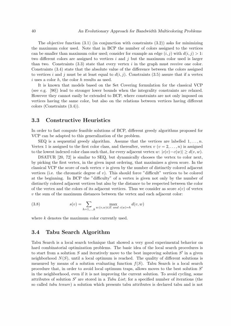
40 An Evolutionary Approach for Bandwidth Multicoloring Problems
The objective function (3.1) (in conjunction with constraints (3.2)) asks for minimizingthe maximum color used. Note that in BCP the number of colors assigned to the verticescan be smaller than maximum color used; consider for example an edge (i, j) with d(i, j) > 1:two different colors are assigned to vertices i and j but the maximum color used is largerthan two. Constraints (3.3) state that every vertex i in the graph must receive one color.Constraints (3.4) state that the absolute value of the difference between the colors assignedto vertices i and j must be at least equal to d(i, j). Constraints (3.5) assure that if a vertexi uses a color h, the color h results as used.
It is known that models based on the Set Covering formulation for the classical VCP(see e.g. [90]) lead to stronger lower bounds when the integrality constraints are relaxed.However they cannot easily be extended to BCP, where constraints are not only imposed onvertices having the same color, but also on the relations between vertices having differentcolors (Constraints (3.4)).
3.3 Constructive Heuristics
In order to fast compute feasible solutions of BCP, different greedy algorithms proposed forVCP can be adapted to this generalization of the problem.
SEQ is a sequential greedy algorithm. Assume that the vertices are labelled 1, . . . , n.Vertex 1 is assigned to the first color class, and thereafter, vertex v (v = 2, . . . , n) is assignedto the lowest indexed color class such that, for every adjacent vertex w: |c(v)−c(w)| ≥ d(v, w).
DSATUR [20, 72] is similar to SEQ, but dynamically chooses the vertex to color next,by picking the first vertex, in the given input ordering, that maximizes a given score. In theclassical VCP the score of each vertex v is given by the number of distinctly colored adjacentvertices (i.e. the chromatic degree of v). This should force ”difficult” vertices to be coloredat the beginning. In BCP the ”difficulty” of a vertex is given not only by the number ofdistinctly colored adjacent vertices but also by the distance to be respected between the colorof the vertex and the colors of its adjacent vertices. Thus we consider as score s(v) of vertexv the sum of the maximum distances between the vertex and each adjacent color:
s(v) =∑
h=1,...,k
maxw:(v,w)∈E and c(w)=h
d(v, w)(3.8)
where k denotes the maximum color currently used.
3.4 Tabu Search Algorithm
Tabu Search is a local search technique that showed a very good experimental behavior onhard combinatorial optimization problems. The basic idea of the local search procedures isto start from a solution S and iteratively move to the best improving solution S′ in a givenneighborhood N(S), until a local optimum is reached. The quality of different solutions ismeasured by means of a solution evaluating function f(S). Tabu Search is a local searchprocedure that, in order to avoid local optimum traps, allows moves to the best solution S′
in the neighborhood, even if it is not improving the current solution. To avoid cycling, someattributes of solution S′ are stored in a Tabu List ; for a specified number of iterations (theso called tabu tenure) a solution which presents tabu attributes is declared tabu and is not

Tabu Search Algorithm 41
considered, except in the case it would improve on the best incumbent solution (aspirationcriterion).
The Tabu Search Algorithm proposed for BCP applies iteratively a Tabu Search Procedure(TS-P) for BCP working in decision version, i.e. requiring as input parameter the maximumcolor k available to color graph G, and returning, if successful, a feasible k coloring. TheTabu Search Algorithm computes an upper bound UB by means of a fast greedy procedure(described in the previous Section), and then calls the Tabu Search Procedure setting themaximum available color k equal to UB − 1, and starting the search from an initial solution.If the problem is solved within a given time limit, k is decreased to k− 1, the time counter isset to zero, and the process is iterated, starting from a new initial solution, until a value ofk is reached for which the procedure is not able to solve the problem within the given timelimit. If one prefers to perform multiple restarts of the Tabu Search Procedure, instead ofusing all the computing time in a single long run, an iteration limit can be used to controlthe execution of the procedure. When the iteration limit is reached and the problem is notyet solved for the given value of k, the Tabu Search Procedure is restarted from scratch, forthe same value of k, starting from a different initial solution. The new initial solution isobtained by means of the constructive heuristics described in the previous Section, which canbe executed with perturbed orderings of the vertices, so as to obtain different solutions.
The Tabu Search Procedure we propose moves between partial k colorings, i.e. solutionsin which the maximum color used is k, all the distance constraints are satisfied, but not all thevertices are colored. For each value of k, the starting partial k coloring is obtained from theinitial solution by ”uncoloring” all the vertices having a color exceeding k. Note that also adummy solution (i.e. a solution in which all the vertices are uncolored) is a partial k coloringwhich can be used as starting k coloring. When all the vertices of G are colored with theavailable k colors (i.e. a feasible k coloring is found), the problem is solved for the given valueof k. The first idea of partial coloring neighborhood was proposed by Morgenstern [92] andwas implemented in Tabu Search procedures for the classical VCP by Blochliger and Zufferey[15] and by Malaguti et al. [84]. In particular, the Tabu Search procedure we propose in thispaper is a generalization of the Tabu Search procedure proposed in [84] for the VCP.
To move from a solution S to a new solution S′ ∈ N(S) one can randomly choose anuncolored vertex v (c(v) = 0), assign v to a color class, say h, and uncolor (i.e. assign to class0) all the vertices w that are adjacent to v and such that |c(w)− h| < d(v, w). This ensuresthat the new solution S′ is still a partial k coloring. Class h is chosen by comparing differenttarget classes, and choosing the class leading to a solution S that minimizes the correspondingvalue of the evaluating function f(S). We do not simply minimize | {v : c(v) = 0} |, becausethis does not consider that some vertices, having an higher degree and larger distances to bemaintained with the adjacent vertices, are more difficult to color. To take into considerationboth aspects we propose the following evaluating function for solution S:
f(S) =∑
v:c(v)=0
∑
w:(v,w)∈E
d(v, w)(3.9)
To avoid cycling, we use the same tabu rule used in [84]: a vertex v cannot take the samecolor h it took in at least one of the last T iterations (where T represents the tabu tenure); forthis purpose we store in a tabu list the pair (v, h) for T iterations. While the move remainstabu, vertex v cannot be assigned to color class h. We also use an Aspiration Criterion: atabu move can be performed if it improves on the best solution encountered so far.
Tabu Search Procedure TS-P takes in input:

42 An Evolutionary Approach for Bandwidth Multicoloring Problems
• a graph G(V, E) with distances on edges;
• the target value k for the maximum color used;
• an initial partial k coloring S := {c(v1), . . . , c(vn)} (obtained by applying a greedyprocedure, see Section 3.3);
• the maximum number L of iterations to be performed;
• the tabu tenure T .
If the procedure solves the problem within L iterations then it gives on output a feasiblek coloring.
Let S be the current solution and S∗ the best incumbent solution. The Tabu SearchProcedure TS-P works as follows:
begin1. S∗ := S;2. tabulist := ∅;3. for ( iterations = 1 to L )4. randomly select an uncolored vertex v (c(v) = 0);5. for each j ∈ {1, . . . , k} (explore the neighborhood of S)6. Sj = (cj(v1), . . . , cj(vn)) := S;7. cj(v) := j;8. for each w : (v, w) ∈ E and |cj(v)− cj(w)| < d(v, w)9. cj(w) := 010. end for11. end for;12. h := arg minj∈{1,...,k}:(v,j)/∈tabulist or f(Sj)<f(S∗) f(Sj);13. if no such h exists then h := arg minj∈{1,...,k} f(Sj);14. S := (c(v1), . . . , c(vn)) := Sh;15. insert (v, h) in tabulist ((v, h) is tabu for T iterations);16. if f(S) < f(S∗) then S∗ := S;17. if {v : c(v) = 0} = ∅ then return S∗
18. end for19. return S∗
end.
At line 12 we try to select the best color class which improves on the best solution so faror does not represent a tabu move. If all moves are tabu, at line 13 we simply select the bestcolor class. In both cases (line 12 and 13), ties are broken by selecting the first best colorclass.
The computational experiments presented in Section 3.6 show that the proposed TabuSearch Algorithm is able to find high quality solutions. However we observed that when, fora given value of k, the Tabu Search Procedure TS-P is not able to solve the problem withinthe given number of iterations L, rarely it is able to find a feasible k coloring, even if moreiterations are allowed. In this case a restart from a different initial solution is usually moreeffective than continuing the search from the current solution. This behavior shows that thesearch strategy is quite aggressive, and able to obtain fast descent of the objective function

The Evolutionary Algorithm 43
in short computing time, but, when the starting solution is in a poor region of the searchspace, the Tabu Search Procedure is not able to escape from this region. More in detail, itcan happen that a vertex v is assigned to a color at the very beginning of the computation,and this choice is never changed during the Tabu Search iterations. These considerationssuggest that a procedure able to extend the search to the whole solution space would be ofgreat efficacy. This procedure is described in the next Section.
3.5 The Evolutionary Algorithm
The Tabu Search Procedure TS-P described in the previous Section can be combined with apopulation management procedure, obtaining a more complex population based EvolutionaryProcedure E-P for BCP. This procedure still works in decision version, and handles a poolof solutions composed by partial k colorings. Like the Tabu Search Procedure TS-P, theEvolutionary Procedure E-P as well can be called iteratively starting from an upper bound, inorder to solve the optimization version of the problem, thus leading to an overall EvolutionaryAlgorithm.
The Evolutionary Procedure E-P works as follows: first an initial pool is defined, i.e. apopulation of solutions (partial k colorings) is initialized by means of fast greedy heuristicalgorithms (see Section 3.3). Then two solutions (parents) are randomly selected from thepopulation and combined through a crossover operator in order to obtain a new solution(offspring). Every offspring solution is improved by means of the Tabu Search Procedure TS-Pbefore to be introduced into the population, replacing the worst parent, i.e. the parent havingthe worst fitness (the fitness of each solution being computed by means of the evaluatingfunction (3.9)). This algorithm can solve both BCP and BMCP, after the transformationof the instances of the latter problem to BCP instances. The algorithm can of course solvealso classical VCP instances, that are a special case of BMCP, arising when all the distancesand weights are equal to 1. However, specialized metaheuristic algorithms designed for theclassical VCP (see e.g. Galinier and Hao [51], Funabiki and Higashino [50], Malaguti et al.[84] for classical metaheuristic approaches; see Barbosa et al. [12] for two novel evolutionaryformulations of the problem and for effective heuristics based on these formulations) have abetter performance, since the crossover operator we propose is based on the tight satisfactionof the distance constraints, and hence it would perform poorly on VCP.
The Evolutionary Procedure E-P takes in input:
• a graph G(V, E) with distances on edges;
• the target value k for the maximum color used;
• the number L of iterations to be performed by procedure TS-P between two calls of thecrossover operator;
• the dimension poolsize of the pool;
• the tabu tenure T ;
• the maximum computing time (timelimit) allowed for the execution of the procedure.
The Evolutionary Procedure E-P is structured as follows:

44 An Evolutionary Approach for Bandwidth Multicoloring Problems
begin1. generate the initial pool containing poolsize solutions (partial k colorings);2. if the problem is solved (i.e. a feasible k coloring is found) during the initialization
then stop;3. while (not timelimit)4. randomly select 2 solutions S1 and S2 from the pool;5. generate S3 := Crossover(S1, S2);6. if the problem is solved then stop;7. [Improve the offspring] S3 := TabuSearch(S3);8. if the problem is solved then stop;9. insert S3 in the pool and delete its worst parent10. end whileend.
3.5.1 Pool Management
We use the Tabu Search Procedure described in Section 3.4 as a component of the morecomplex Evolutionary Procedure, where a pool of different solutions is managed, and solutionsare combined, by means of a crossover operator, in order to generate new solutions. Thesenew solutions can be used as starting points to extend the Tabu Search to different regions ofthe whole solution space. In this framework, the Tabu Search Procedure is used to improveon the quality of the different solutions of the pool.
The use of Pool Management procedures is justified by the experimental observation that,given a fixed number of Tabu Search iterations to be executed, it is better to perform multiplerestarts from different initial solutions than to spend all the available iterations in a singlerun. Indeed, the Tabu Search Procedure seems unable to move away from a limited regionof the solution space, and the final solution is usually close to the initial one. At the sametime, a naive multiple restart strategy does not intensify the search in more promising regionsof the solution space. Thus we use a specialized crossover operator to generate new startingsolutions, sharing interesting properties with their parents, and we improve these solutions bymeans of the Tabu Search Procedure. It is known that generic crossover operators performpoorly on VCP (see, e.g., Davis [38]), while it was experimentally shown that specializedcrossover operators can be effective in the case of the classical VCP (see [51, 84]), and thecomputational experiments presented in Section 3.6 show that this is true in the case of VCPgeneralizations as well. The main idea behind the use of a specialized crossover operator is that”good” solutions share part of their structure with the optimal ones, and that a specializedcrossover is generally able to identify properties that are meaningful for the problem.
Initialization
During the initialization phase of the Evolutionary Procedure E-P, we generate poolsize initialsolutions (partial k colorings) that will be handled by the Pool Management procedures andimproved by means of the Tabu Search Procedure. For the success of the overall search it iscrucial to start with solutions having different structures, thus allowing the Pool Managementprocedures to access the whole solution space, by recombining solutions through the crossoveroperator.
To diversify as much as possible the solutions contained in the initial pool, during the

The Evolutionary Algorithm 45
initialization phase we use three different algorithms: two thirds of the solutions are generatedby applying the two greedy algorithms SEQ and DSATUR described in Section 3.3; the lastthird is generated by the Tabu Search Procedure TS-P applied starting from a dummy solution(all vertices uncolored) and maximum number k of colors. The three algorithms are appliedwith different random orderings of the vertices, so as to generate different solutions. To obtainpartial k colorings, all the vertices colored by the greedy algorithms with colors greater thank are uncolored before to insert the corresponding solution in the pool.
Every initial solution generated by SEQ or DSATUR is improved by means of the TabuSearch Procedure before to be inserted in the pool.
Solutions Selection
Once the pool of solutions is initialized, two solutions must be selected and combined toextend the search. The solutions to be combined through the crossover operator are randomlychosen among the solutions of the pool. The new offspring solution, improved by means of theTabu Search Procedure, is then introduced into the population, replacing the parent whichresults to have the worst fitness with respect to the solution evaluating function (3.9) used inthe Tabu Search Procedure.
Crossover Operators
An effective crossover operator must take in input two parent solutions S1 and S2 andtransmit to the offspring solution S3 the parents’s properties that are meaningful for theproblem. In the case of the classical VCP, the structure of a solution is given by the partitionof the vertices into independent sets (each corresponding to a different color). The color thatis given to a set is completely arbitrary. This leads to very effective crossover operators wherenew solutions are built by combining the independent sets of the corresponding parents (see[51, 84]).
In the case of BCP, the color that is assigned to each set of vertices, with respect to theother sets, becomes important for the feasibility of the solution, as imposed by the distanceconstraints. Thus the structure of a solution is given not only by the partition of the verticesinto independent sets, but by the mutual distances between colored vertices as well.
We computationally experimented different crossover operators that, given two parentsolutions S1 and S2 represented by partial k colorings, output as offspring a partial k coloringS3. The characteristics of these crossovers are summarized in the following:
• Crossover #1: Given two parents S1 and S2, the color classes of the offspring S3 are builtby iteratively picking the color class of maximum cardinality from one parent (in turnS1 or S2) and assigning the corresponding vertices to the offspring. These vertices areinserted in the first free color class of S3, starting from color 1, if they do not violate thedistance constraints. Every vertex violating the distance constraints, as well as verticesuncolored in both parents, are left uncolored. The inserted vertices are then deletedfrom the other parent. The process is iterated from the other parent while there areavailable colors in the offspring. This crossover was designed for VCP (see [51, 84] formore details) and gives poor performance in the case of BCP, due to the fact that manyvertices cannot be colored in the offspring without violating the distance constraints.

46 An Evolutionary Approach for Bandwidth Multicoloring Problems
• Crossover #2: This crossover is similar to crossover #1, but, in this case, the colorclasses of the offspring are filled in the following order: 1, k, 2, k − 1, etc. This way offilling the color classes generally reduces the number of vertices that cannot be coloredin the offspring because of the distance constraints.
• Crossover #3: This crossover as well is similar to crossover #1, but, in this case, themaximum cardinality color class picked from the parent is forced to keep the sameposition (color) when copied to S3. This choice generally avoids the infeasibilities be-tween color classes picked from the same parent, thus reducing the number of uncoloredvertices in the offspring.
• Crossover #4: Fixed a value p, a given percentage p of the vertices of the offspringS3, randomly selected, are colored with the same color they have in S1, the remainingpercentage 1 − p is colored with the color they have in S2, if this does not violate thedistance constraints.
• Crossover #5: Fixed a value h, the first h color classes of parent S1 are copied to theoffspring S3, the last k − h color classes of S2 (with the exception of already coloredvertices) are copied to S3, leaving uncolored the vertices that would violate the distanceconstraints.
By considering the test instances described in Section 3.6, we observed that the last twocrossovers perform better than the previous ones, but their performance is not comparablewith that of the crossover we finally included in our algorithm and that was extensively testedas reported in Section 3.6.2. We call it distance crossover because it is based on the ideathat the important structure to be transferred from the parents to the offspring is the relativecolor distance between the vertices, in particular when the distance constraints are satisfiedtightly. The distance crossover works as follows (let c1(v), c2(v) and c3(v) denote the colorassigned to vertex v ∈ V in solution S1, S2 and S3, respectively; initially all the vertices inS3 are uncolored):
begin1. E1 := {(v, w) ∈ E : v < w, |c1(v)− c1(w)| = d(v, w)};2. for each (v, w) ∈ E1 : c3(v) := c1(v), c3(w) := c1(w);3. E2 := {(v, w) ∈ E : v < w, |c2(v)− c2(w)| = d(v, w)};4. for each (v, w) ∈ E2:5. if both v and w are currently uncolored in S3:6. if feasible, set c3(v) = c2(v); c3(w) = c2(w) ;7. else try to color v and w with any color, starting from 1,
still maintaining |c3(v)− c3(w)| = d(v, w)8. else if one vertex of the pair (v,w)(say v) is already colored:9. if feasible, set c3(w) := c3(v) + d(v, w)10. else if feasible, set c3(w) := c3(v)− d(v, w)11. end forend.
We copy all the ”tight distance” pairs from S1 to the offspring, keeping the same colorassignment. Then we try to do the same with ”tight distance” pairs from S2, keeping the

Computational Analysis 47
same color assignment, when this does not violate the distance constraints with respect tothe already colored vertices of the offspring. As in the other crossovers that we experimented,when a vertex cannot feasibly be colored, or it was uncolored in both parents, we leave ituncolored.
After the crossover, that is mainly aimed at generating new solutions, sharing importantstructures with their parents (and not simply at generating an offspring with many coloredvertices), we could use a greedy algorithm in order to color uncolored vertices. We prefer toleave these vertices uncolored and directly apply the Tabu Search Procedure to the offspringS3, which will insert the uncolored vertices in the first color class where they can be insertedwithout moving other vertices (if any).
3.6 Computational Analysis
The Tabu Search Algorithm and the Evolutionary Algorithm described, respectively, in Sec-tions 3.4 and 3.5 were coded in ANSI C and compiled with full optimization option. Theprograms were run on a PIV 2.4MHz computer, with 512MB RAM, under Windows XP,and tested on the instances proposed during the Computational Symposium on Graph Col-oring and its Generalizations, held in 2002. These instances (which can be found at [106])correspond to different graph types used for evaluating the performance of VCP algorithms.To perform our computational experiments, we considered the instance sets GEOMn, GE-OMna and GEOMnb (where n represents the number of vertices of the graph), proposed forBCP and BMCP. In these geometric graphs, the vertices are uniformly randomly generatedin a 10,000 by 10,000 grid, and are connected by an edge if they are close enough. Edgedistances are inversely proportional to the Euclidean distance between the corresponding ver-tices. Vertex weights are uniformly randomly generated, between 1 and 10 for sets GEOMnand GEOMna, and between 1 and 3 for set GEOMnb. GEOMn instances correspond to sparsegraphs; GEOMna and GEOMnb instances correspond to denser graphs. We also consideredthe Philadelphia instances [9], that were extensively studied in the MS-FAP literature (see,e.g., [4]). In these BMCP instances, each of the 21 vertices of the graph must receive a largenumber of colors (32.2 on average).
All the computing times reported in this section are expressed in seconds of our machine.To allow a meaningful - although approximate - comparison on results obtained with differentmachines, a benchmark program (dfmax), together with a benchmark instance (r500.5), areavailable. Computing times obtained on different machines can be scaled with respect to theperformance obtained on this program (our machine spent 7 seconds ”user time”).
3.6.1 Performance of the Tabu Search Algorithm
In this section we report the experimental results obtained by the Tabu Search Algorithm(described in Section 3.4) on the BCP and BMCP instances presented in [106]. In order tofast compute an initial upper bound UB, we perform 20 runs of the greedy algorithm SEQ(described in Section 3.3), with perturbed input orderings of the vertices, and set UB equalto the best solution value found. As explained in Section 3.4, we run the Algorithm withmultiple restarts of the Tabu Search Procedure TS-P. The maximum number of iterations Lof the Tabu Search Procedure TS-P is set to 100,000 in the case of BCP, and to 400,000 inthe case of BMCP. After L iterations, if the problem is not solved for the current value of k,we restart procedure TS-P from a new solution (partial k coloring). Every partial k coloring

48 An Evolutionary Approach for Bandwidth Multicoloring Problems
is obtained in turn by applying the SEQ or DSATUR algorithms, where we uncolor all thevertices whose current color exceeds the given k value, or starting from a dummy solution (allvertices uncolored). If we are able to solve the problem, for the current value of k, within thetime limit (which is set to 500 seconds in the case of BCP and to 3000 seconds in the caseof BMCP), we decrease the value of k and set to zero the time counter. We iterate until, forthe current value of k, the problem cannot be solved within the time limit.
In Table 3.1 we report, for every considered BCP instance from [106], the name of theinstance, the number of vertices (n) and edges (m) of the considered graph, the best knownsolution value ever published in the literature [93, 95, 82, 96, 81] (”best”), the initial upperbound found by the SEQ algorithm (”UB”), the solution value (”k”), the number of iter-ations needed to find the last improving solution starting from the initial UB (”iter”), thetotal computing time (including the initial UB computation) corresponding to the last im-provement (”time”, we report 0 when the time is lower than 1 second). The tabu tenure T isfixed to a value of 50 for the BCP instances, while better results can be obtained in the caseof the BMCP instances with a tabu tenure T equal to the number of vertices of the graph,after the transformation described in Section 3.1. In Table 3.2 we report the results obtainedon the BMCP instances. The last two rows of Tables 3.1 and 3.2 report the average ratiobetween the solution value and the best known solution value from the literature (k/best)and the average computing time.
For the set-up of the parameters T and L, we selected the values that, on different com-putational tests performed, lead on average to the best results in terms of solution value andtime. Of course, better results can be obtained by using an ad hoc set up tuned on eachinstance, but our opinion is that the robustness of the algorithm, i.e. the capacity of solvingdifferent instances without requiring a special set-up on each instance, has to be preferred.
The Tabu Search Algorithm we propose has a very good experimental behavior in thecase of BCP (Table 3.1). The quality of the solutions found is comparable with that of thesolutions found by the state of the art algorithms. Over 33 considered instances, the TabuSearch Algorithm is able to improve on the best published solution in the literature 4 times,in 21 cases it finds a solution whose value equals the best published one and in the remaining8 cases it is worse, but always using only one more color. Also in the case of BMCP (Table3.2) the quality of the solutions found is comparable with that of the solutions found by thestate of the art algorithms. Over 33 considered instances, the Tabu Search Algorithm is ableto improve on the best published solution in the literature 8 times, in 11 cases it finds asolution whose value equals the best published one, and in the remaining 14 cases it is worse.
We tested the Tabu Search Algorithm also on the 9 Philadelphia instances [9], representingBMCP instances corresponding to the Minimum Span Frequency Assignment Problem (MS-FAP), where 21 vertices must receive a large number of colors (32.2 on average). As it couldbe expected, our algorithm performs very poorly on these instances, obtaining solutions valuesthat are on average 6.5% larger than the optimal ones (which are known, and can be found byspecialized metaheuristics approaches, see [4]). This is due to the extra symmetry introducedin the problem by transforming BCMP instances to BCP ones, i.e. by transforming eachvertex i which must receive w(i) colors to a clique of cardinality w(i). This transformationleads to BCP instances where our approach is completely ineffective, because large cliquesare built, and our Tabu Search approach risks to spend all the iterations by moving verticesof the same clique (representing originally a single vertex) to different color classes, withoutreally changing the solution.

Computational Analysis 49
Table 3.1: Tabu Search Algorithm: Bandwidth Coloring Instances.Instance name n m best UB k iter time
GEOM20 20 40 20 21 21 0 0GEOM20a 20 57 20 22 20 1613 0GEOM20b 20 52 13 15 13 10 0GEOM30 30 80 27 28 28 0 0GEOM30a 30 111 27 31 27 13051 0GEOM30b 30 111 26 26 26 0 0GEOM40 40 118 27 29 28 15 0GEOM40a 40 186 37 41 37 24753 0GEOM40b 40 197 33 40 33 3745 0GEOM50 50 177 28 29 28 697 0GEOM50a 50 288 50 55 50 32125 0GEOM50b 50 299 35 44 35 500360 0GEOM60 60 245 33 35 33 3038 0GEOM60a 60 339 50 57 50 24038 0GEOM60b 60 426 43 54 41 96611523 147GEOM70 70 337 38 42 38 2021 0GEOM70a 70 529 62 70 61 15810658 29GEOM70b 70 558 48 62 48 44923788 76GEOM80 80 429 41 46 41 76460 0GEOM80a 80 692 63 77 63 4474619 9GEOM80b 80 743 61 78 61 14347412 30GEOM90 90 531 46 50 46 10594 0GEOM90a 90 879 64 77 63 32340177 73GEOM90b 90 950 72 89 72 17708445 47GEOM100 100 647 50 58 50 1184211 2GEOM100a 100 1092 68 89 69 33992244 73GEOM100b 100 1150 73 96 74 45945300 114GEOM110 110 748 50 60 50 371993 1GEOM110a 110 1317 73 94 74 570556 1GEOM110b 110 1366 79 105 79 129462538 338GEOM120 120 893 60 70 59 1975913 3GEOM120a 120 1554 84 103 85 202323831 470GEOM120b 120 1611 86 116 87 18180399 50
avg. gap (k/best) 1.0029avg. time 44

50 An Evolutionary Approach for Bandwidth Multicoloring Problems
Table 3.2: Tabu Search Algorithm: Bandwidth Multicoloring Instances.Instance name n m best UB k iter time
GEOM20 20 40 149 155 149 939426 3GEOM20a 20 57 169 176 169 123721114 405GEOM20b 20 52 44 46 44 10552157 13GEOM30 30 80 160 172 160 195505 1GEOM30a 30 111 209 242 211 767838021 3684GEOM30b 30 111 77 79 77 121319 0GEOM40 40 118 167 180 167 4416693 18GEOM40a 40 186 213 230 215 302864957 1639GEOM40b 40 197 74 87 74 160164 1GEOM50 50 177 224 235 225 24019956 130GEOM50a 50 288 318 359 320 102725774 792GEOM50b 50 299 86 103 83 118972111 304GEOM60 60 245 258 266 258 40375817 202GEOM60a 60 339 358 404 363 764735785 5632GEOM60b 60 426 116 139 114 878357241 2969GEOM70 70 337 273 312 270 251841925 1487GEOM70a 70 529 469 509 473 106820588 1084GEOM70b 70 558 119 142 119 62714747 208GEOM80 80 429 383 422 388 269267418 2088GEOM80a 80 692 379 406 370 154315259 1530GEOM80b 80 743 141 164 141 95766220 330GEOM90 90 531 332 354 334 197265420 1460GEOM90a 90 879 377 416 384 352269766 3024GEOM90b 90 950 147 178 146 36450728 153GEOM100 100 647 404 424 412 439473614 3425GEOM100a 100 1092 453 507 452 437615679 4471GEOM100b 100 1150 159 201 160 163576744 804GEOM110 110 748 383 421 382 748917011 7325GEOM110a 110 1317 494 535 492 40969388 455GEOM110b 110 1366 206 240 207 108643060 645GEOM120 120 893 402 430 405 333840804 2718GEOM120a 120 1554 556 611 559 257342109 3149GEOM120b 120 1611 195 224 195 176508745 951
avg. gap (k/best) 1.0009avg. time 1548

Computational Analysis 51
3.6.2 Performance of the Evolutionary Algorithm
In this section we describe the experiments performed with the Evolutionary Algorithm (de-scribed in Section 3.5) and compare it with the most effective algorithms proposed in theliterature on the BCP and BMCP instances presented in [106]. The corresponding computa-tional results are reported, respectively, in Tables 3.3 and 3.4. The first two columns of thetables report the instance name and the corresponding best published solution value (”best”).
The solution values (”k”) and the corresponding computing times obtained by Lim et al.[82], with an algorithm combining hill-climbing techniques and Squeaky Wheel Optimization,are reported in the third and forth columns of Tables 3.3 and 3.4. The algorithm works inoptimization version (i.e. it does not require as input the maximum color k to be used). Wereport the best solution value found over a single run and the computing time needed to getthis result, scaled with respect to the time obtained on the benchmark problem (25.32 seconds”user time”), and thus directly comparable with the other reported times.
The fifth column of Table 3.3 reports the solution values (”k”) obtained by Phan andSkiena by means of the Discropt general heuristic [93] in the case of BCP (they reportno results for BMCP). The algorithm works in optimization version. The reported resultsrepresent the best value obtained over 3 runs, using 3 different versions of the algorithm.The total computing time was 300 seconds (100 seconds for each run), on a Athlon K7 AMDprocessor with 768 MB of RAM under RedHat 7.2.
The solution values (”k”) and the corresponding computing times obtained by Lim etal. [81], with an algorithm combining Squeaky Wheel Optimization with Tabu Search, arereported in the fifth and sixth columns of Table 3.4 in the case of BMCP (results for BCP arenot competitive and were not reported in detail in [81]). The algorithm works in optimizationversion. We report, for each instance, the best solution value found over a run with 10 restartsand the computing time needed to get this result, scaled with respect to the time obtainedon the benchmark problem (74.12 seconds ”user time”).
The solution values (”k”) and the corresponding computing times obtained by Prestwichwith an algorithm which hybridizes Local Search and Constraint Programming [96] are re-ported in the sixth and seventh columns of Table 3.3 in the case of BCP, and in the seventhand eighth columns of Table 3.4 in the case of BMCP. The times are scaled with respect tothe time obtained on the benchmark problem (27.43 seconds ”user time”). The algorithm,working in optimization version, requires some input parameters, whose values are tuned,among a limited set of possibilities, for each instance.
Finally we report the results obtained by means of the Evolutionary Algorithm, used tosolve the optimization version of the problem. Like we did with the Tabu Search Algorithm,we compute an initial upper bound UB by performing 20 runs of the greedy algorithm SEQ(described in Section 3.3), with perturbed input orderings of the vertices, and set UB equalto the best solution value found.
Then, like in the case of the Tabu Search Algorithm, we run the Evolutionary Algorithm,trying to improve on this UB. We use a time limit, for every value of k, of 500 seconds inthe case of BCP and of 3000 seconds in the case of BMCP. If the problem is solved, for thecurrent value of k, we decrease it to k − 1 and set to zero the time counter. We iterate until,for the current value of k, the problem cannot be solved within the time limit.
The last columns of Table 3.3 and Table 3.4 report the results obtained by the EvolutionaryAlgorithm in the case of BCP and BMCP, respectively. We report the solution value (”k”),the number of iterations needed to find the last improving solution starting from the initial

52 An Evolutionary Approach for Bandwidth Multicoloring Problems
UB (”iter”), the total computing time (including the initial UB computation) correspondingto the last improvement, and the difference between the solution value (”k”) and the bestsolution value (”best”) published in the literature on instances from [106]. The value of theinitial upper bound UB and the setting of the tabu tenure T are equal to those used forthe Tabu Search Algorithm. The poolsize was fixed to a value of 40 for both BCP andBMCP. Instead of performing multiple restarts, the Evolutionary Algorithm calls the crossover operator. The number of iterations (L) of the Tabu Search Procedure, between twoconsecutive calls of the cross over operator, is equal to that used when testing multiple restartsfor the Tabu Search Algorithm, i.e. 100,000 in the case of BCP and 400,000 in the case ofBMCP. The use of the same set-up of the parameters T and L and of the same time limitshould ensure a fair comparison between the Tabu Search Algorithm and the EvolutionaryAlgorithm.
The last two rows of Tables 3.3 and 3.4 report, for each considered algorithm, the aver-age ratio between the solution value and the best known solution value from the literature(k/best), and the average computing time.
Over the 33 considered instances of BCP, the Evolutionary Algorithm is able to improve onthe best published solution in the literature 9 times, in 21 cases it finds a solution whose valueequals the best published one, and in the remaining 3 cases it is worse. It clearly outperformsthe other proposed algorithms, singularly considered, from the point of view of the solutionquality. The computing times are much longer, but, in our opinion, acceptable, since theyimprove on the best known solutions. The Evolutionary Algorithm improves 8 times on thebest solution found by using the Tabu Search Algorithm, thus showing the efficacy of theoverall diversification approach with respect to a simple multiple restart strategy.
Over the 33 considered instances of BMCP, the Evolutionary Algorithm is able to improveon the best published solution in the literature 13 times, in 13 cases it finds a solution whosevalue equals the best published one, and in the remaining 7 cases it is worse. Its performance,from the solution quality point of view, is better than that of the best considered algorithm,namely the one proposed by Lim et al. [81]. The latter finds 7 times a better solution thanthe one found by the Evolutionary Algorithm, while 13 times the proposed algorithm findsa better solution. Our computing times are in general larger on bigger instances, but stillacceptable. The Evolutionary Algorithm improves 17 times on the best solution found byusing the Tabu Search Algorithm, while the latter finds 3 times a better solution. This showsagain the efficacy of the overall diversification approach with respect to a simple multiplerestart strategy.
In our experiments, we used time limits which lead to long computational times withrespect to other algorithms proposed in the literature: we think that this choice is justified,since we are able to improve some of the best know solution values published in the literature.It must be observed that the hard part of the computation very often corresponds to thoseimprovements. In other words, when we spend a long time to improve the best known solutionvalue of only few colors, a large part of the computation is devoted to solve the problem for thelast values of k. This means that, when shorter computing times are imposed, our algorithmis still able to find feasible solutions of good quality. During our experiments, we observedthat allowing even longer time limits would lead to better solutions on some instances, butwith an average computational cost exceeding the acceptable threshold.
We tested the Evolutionary Algorithm also on the 9 Philadelphia (MS-FAP) instances,obtaining solution values that are on average 6.6% far from the optimal ones. This behavior,due to the transformation of BMCP instances to BCP instances, should not surprise, as

Conclusions 53
discussed in the previous Section.
3.7 Conclusions
In this paper we present an Evolutionary heuristic algorithm for two generalizations of thewell known VCP, namely the Bandwidth Coloring (BCP) and the Bandwidth Multicoloring(BMCP) Problems. The Algorithm was designed for BCP, and applied to BMCP instances aswell (after their transformation to BCP instances by means of a simple procedure). The Evo-lutionary Algorithm proposed to solve the BCP combines an effective Tabu Search approachwith a specialized crossover operator.
Extensive computational experiments on 66 BCP and BMCP instances from literaturebenchmark graphs were performed with the Tabu Search approach and the overall Evolu-tionary Algorithm. The first is able to produce very good solutions in acceptable computingtimes. Improved solutions can be obtained by using the overall Evolutionary Algorithm. Thecomparison of the latter with the most effective algorithms from the literature shows thatthe proposed approach represents, on the considered set of instances, the new state of the artheuristic algorithm for BCP, and equals the most effective algorithm for BMCP.
Instances of BMCP corresponding to Frequency Assignment problems were also consid-ered, where our approach performed very poorly. This behavior can be explained by consid-ering the structure of these instances, where the transformation of BMCP to BCP was veryineffective, because it introduced much extra symmetry into the model.
Thus, in order to overcome this limit of our approach, in future work we intend to tacklethe Multicoloring Problems solving directly a Multicoloring model.

54 An Evolutionary Approach for Bandwidth Multicoloring Problems
Table 3.3: Performance of the Evolutionary Algorithm and comparison with the most effectiveheuristic algorithms for the Bandwidth Coloring Problem.
Lim et al. Phan and Skiena Prestwich Evolutionary2003 [82] 2002 [93] 2005 [96]
Instance name best k time k k time k iter time diff.
GEOM20 20 21 0 20 21 0 21 0 0 1GEOM20a 20 22 0 20 20 0 20 1730 0 0GEOM20b 13 14 0 13 13 0 13 6 0 0GEOM30 27 29 0 27 28 0 28 0 0 1GEOM30a 27 32 0 27 27 0 27 13064 0 0GEOM30b 26 26 0 26 26 0 26 0 0 0GEOM40 27 28 1 27 28 0 28 479 0 1GEOM40a 37 38 1 38 37 0 37 24428 0 0GEOM40b 33 34 1 36 33 0 33 3750 0 0GEOM50 28 28 1 29 28 0 28 214 0 0GEOM50a 50 52 1 54 50 2 50 36707 0 0GEOM50b 35 38 2 40 35 0 35 326548 0 0GEOM60 33 34 0 34 33 0 33 3364 0 0GEOM60a 50 53 2 54 50 1 50 23812 0 0GEOM60b 43 46 1 47 43 0 41 18739807 29 -2GEOM70 38 38 0 40 38 0 38 2036 0 0GEOM70a 62 63 0 64 62 2 61 6746180 12 -1GEOM70b 48 54 0 54 48 1 48 30608071 52 0GEOM80 41 42 2 44 41 0 41 76891 0 0GEOM80a 63 66 0 69 63 12 63 75341752 150 0GEOM80b 61 65 8 70 61 0 60 69418472 145 -1GEOM90 46 46 0 48 46 3 46 10755 0 0GEOM90a 64 69 2 74 64 2 63 66256099 150 -1GEOM90b 72 77 6 83 72 2 70 376194388 1031 -2GEOM100 50 51 9 55 50 0 50 1296142 2 0GEOM100a 68 76 6 84 68 9 68 125814038 273 0GEOM100b 73 83 2 87 73 15 73 235521605 597 0GEOM110 50 53 1 59 50 4 50 1824578 3 0GEOM110a 73 82 11 88 73 7 72 72749430 171 -1GEOM110b 79 88 5 87 79 2 78 246378762 676 -1GEOM120 60 62 0 67 60 4 59 293669 0 -1GEOM120a 84 92 1 101 84 4 84 263039830 614 0GEOM120b 86 98 1 103 86 9 84 304671189 857 -2
avg. ratio (k/best) 1.0646 1.0906 1.0054 0.9980avg. time 2 2.5 144

Conclusions 55
Table 3.4: Performance of the Evolutionary Algorithm and comparison with the most effectiveheuristic algorithms for the Bandwidth Multicoloring Problem.
Lim et al. Lim et al. Prestwich Evolutionary2003[82] 2005[81] 2005[96]
Instance name best k time k time k time k iter time diff.
GEOM20 149 149 0 149 17 149 4 149 5293853 18 0GEOM20a 169 169 4 169 16 170 2 169 2400000 9 0GEOM20b 44 44 0 44 2 44 0 44 3203748 5 0GEOM30 160 160 0 160 23 160 0 160 195203 1 0GEOM30a 209 211 3 209 40 214 11 210 166234965 954 1GEOM30b 77 77 0 77 7 77 0 77 112224 0 0GEOM40 167 167 1 167 47 167 1 167 4969719 20 0GEOM40a 213 214 99 213 54 217 299 214 75188430 393 1GEOM40b 74 76 2 74 10 74 4 74 160125 1 0GEOM50 224 224 11 224 77 224 1 224 247423944 1197 0GEOM50a 318 326 27 318 12 323 51 316 600574823 4675 -2GEOM50b 86 87 15 87 15 86 1 83 72424865 197 -3GEOM60 258 258 13 258 96 258 77 258 27935150 139 0GEOM60a 358 368 1037 358 162 373 10 357 1161910138 8706 -1GEOM60b 116 119 83 116 23 116 12 115 134011555 460 -1GEOM70 273 279 7 273 138 277 641 272 220981847 1413 -1GEOM70a 469 478 115 469 188 482 315 473 97340773 988 4GEOM70b 119 124 38 121 30 119 55 117 222025798 897 -2GEOM80 383 394 1118 383 204 398 361 388 16559905 132 5GEOM80a 379 379 187 379 190 380 109 363 1042840998 8583 -16GEOM80b 141 145 894 141 39 141 37 141 443911693 1856 0GEOM90 332 335 1133 332 248 339 44 332 579637236 4160 0GEOM90a 377 382 2879 377 245 382 13 382 631825295 5334 5GEOM90b 147 157 179 157 46 147 303 144 417466073 1750 -3GEOM100 404 413 175 404 311 424 7 410 422527570 3283 6GEOM100a 453 462 48 459 334 461 26 444 1259264110 12526 -9GEOM100b 159 172 1354 170 55 159 367 156 755603823 3699 -3GEOM110 383 389 160 383 368 392 43 383 240024033 2344 0GEOM110a 494 501 1292 494 441 500 29 490 186931545 2318 -4GEOM110b 206 210 3 206 68 208 5 206 82617492 480 0GEOM120 402 409 505 402 408 417 9 396 349961343 2867 -6GEOM120a 556 564 1476 556 633 565 41 559 327849778 3873 3GEOM120b 195 201 240 199 97 196 3 191 613183196 3292 -4
avg. ratio (k/best) 1.0181 1.0060 1.0120 0.9954avg. time 397 141 87 2320

56 An Evolutionary Approach for Bandwidth Multicoloring Problems

Chapter 4
Models and Algorithms for aWeighted Vertex Coloring Problem
1
We consider a weighted version of the well-known Vertex Coloring Problem (VCP) inwhich each vertex i of a graph G has associated a positive weight wi. Like in VCP, oneis required to assign a color to each vertex in such a way that colors on adjacent verticesare different, and the objective is to minimize the sum of the costs of the colors used. Thedifference with respect to VCP is that the cost of each color is given by the maximum weightof the vertices assigned to that color. The corresponding problem is known to be NP-hard andarises in practical scheduling applications, where it is also known as Scheduling on a BatchMachine with Job Compatibilities. We propose a straightforward formulation for WVCP, andtwo alternative Integer Linear Programming (ILP) models: the first one is used to derive,dropping integrality requirement for the variables, a tight lower bound on the solution value,while the second one is used to derive a 2-phase heuristic algorithm, also embedding fastrefinement procedures aimed at improving the quality of the solutions found. Computationalresults on a large set of instances from the literature are reported.
4.1 Introduction
We approach a weighted version of the well known Vertex Coloring Problem (VCP), wherean undirected graph G = (V,E) is given (with V denoting the vertex set, and E the edgeset) and each vertex i ∈ V has associated a positive weight wi. Like in the classical VCP,one has to assign a color to each vertex i in such a way that colors on adjacent vertices aredifferent. The objective of this Weighted Vertex Coloring Problem (WVCP) is to minimizethe sum of the costs of the colors used, where the cost of each color is the maximum weightof the vertices assigned to the color (while in the classical VCP the cost of each color is equalto one, thus the total number of colors has to be minimized).
WVCP is known to be strongly NP-hard since it generalizes VCP (see Garey and Johnson[53] for complexity results on VCP). De Werra, Demange, Monnot and Paschos [40] ana-lyzed some properties of the optimal solutions and discussed complexity and approximabilityresults for this problem, Escoffier, Monnot and Paschos [45] continued the investigation of
1Preliminary results of this chapter appear in [85].
57

58 Models and Algorithms for a Weighted Vertex Coloring Problem
the complexity and the approximability of WVCP, while Boudhar and Finke [19] studied itscomplexity for several classes of graphs. These results were extended to different classes ofgraphs by Finke, Jost, Queyranne and Sebo [48].
WVCP has many real world applications in different industrial fields. In the schedulingliterature it is also known as Scheduling on a Batch Machine with Job Compatibilities, andit generalizes some applications where a compatibility graph limits the simultaneous accessto a resource by the users. A typical case, concerning thermic treatment or mechanicalprocessing, arises when some jobs cannot be processed within the same time slot because ofgeometric constraints (see Gavranovich and Finke [54]), and the duration of each time slotcorresponds to the maximum processing time of the associated jobs. This kind of temporalconstraint was studied by Hochbaum and Landy [63], who considered an application dealingwith semiconductor burn-in operations in which the capacity of the oven limits the numberof jobs that can be processed within the same time slot.
WVCP is also a generalization of the Matrix Decomposition Problem in Time DivisionMultiple Access Traffic Assignment (see Ribeiro, Minoux and Penna [99] and Prais and Ribeiro[94]), where a traffic matrix has to be decomposed into mode matrices (i.e., matrices such thatno more than a non zero element is present in each row and column), and the transmissiontime of each mode matrix equals the maximum of its non zero elements. An exact approachto the Matrix Decomposition Problem, based on column generation, was proposed in [99],while in [94] a heuristic approach based on a Greedy Randomized Adaptive Search Procedure(GRASP) is presented.
Some definitions will be used in the following: let n and m be the cardinalities of vertexset V and edge set E, respectively.A clique of a graph G is a complete subgraph of G. Asubset of V is called an independent set if no two adjacent vertices belong to it. The stabilitynumber α is the cardinality of the largest independent set of the graph. Note that eachcoloring of a graph is a partition of the vertex set into independent sets; we will call thesesets color classes. An independent set (resp. clique) is maximal if no vertex can be addedstill having an independent set (resp. clique). Given an independent set s ⊆ V of weightedvertices, we define its cost cs as the maximum weight of its vertices. We say that independentset s dominates independent set t if t ⊂ s and cs = ct. An independent set t is said to be nondominated if no independent set s exists that dominates t. Given a (possible partial) coloringof G, the chromatic degree δχ(i) of a vertex i ∈ V is the number of different colors assignedto its adjacent vertices.
In the following we will assume, without loss of generality, that all weights wi are positiveintegers, and that vertices are numbered in such a way that
w1 ≥ w2 ≥ . . . ≥ wn.(4.1)
The paper is organized as follows: in the next Section we propose different Integer LinearProgramming (ILP) models for the problem: Section 4.2.1 presents a straightforward ILPmodel, while Section 4.2.2 introduces a new ILP formulation, whose LP relaxation dominatesthe LP relaxation of the first model (see Section 4.2.3). Finally, Section 4.2.4 presents a thirdILP model, involving an exponential number of variables, which is used to derive a 2-phaseheuristic approach, outlined in Section 4.3: constructive heuristics used in the first phaseare described in Section 4.3.1, Section 4.3.2 describes the second phase of the algorithm,and Section 4.4 presents post-optimization procedures aimed at improving the quality of thesolutions found. Computational experiments on a wide set of instances from the literatureare reported in Section 4.5. Concluding remarks are discussed in Section 4.6.

ILP models 59
4.2 ILP models
We first describe two alternative ILP formulations for WVCP, involving a polynomial numberof variables and constraints, and analyze the relation between the optimal solution values ofthe LP relaxations of the models, since such values are valid lower bounds for WVCP. Further,we present another ILP formulation that involves an exponential number of variables, andthat is used for designing a heuristic algorithm.
4.2.1 Model M1
Noting that the number of colors in any feasible solution cannot be larger than n, we canrestrict our attention to solutions involving up to n colors. Hence, a straightforward ILPmodel for WVCP can be obtained by defining the following two sets of variables: binaryvariables xih (i ∈ V, h = 1, . . . , n), with xih = 1 iff vertex i is assigned to color h, and(continuous) variables zh (h = 1, . . . , n) denoting the cost of color h in the solution.
The corresponding model for WVCP is:
(M1) minn∑
h=1
zh(4.2)
zh ≥ wi xih, i ∈ V, h = 1, . . . , n,(4.3)n∑
h=1
xih = 1, i ∈ V,(4.4)
xih + xjh ≤ 1, (i, j) ∈ E, h = 1, . . . , n,(4.5)xih ∈ {0, 1}, i ∈ V, h = 1, . . . , n.(4.6)
Objective function (4.2) minimizes the sum of the costs of the colors, which are definedby constraints (4.3). Constraints (4.4) require that every vertex is given a color, while (4.5)impose that adjacent vertices cannot receive the same color. Finally, constraints (4.6) requirex variables to be binary.
This formulation is the most natural way to model problems in which one is required topartition a given set of items into subsets, the feasibility and cost of each subset dependingonly on the items assigned to the subset itself. However, this formulation tends to performpoorly in practice, mainly for two reasons. The first drawback of this model arises whenone wants to solve the ILP above, since the solution space contains many optimal solutionsdue to symmetries. Indeed, given a feasible solution to (4.2)–(4.6), another feasible solutionhaving the same cost is obtained by permuting the selected color classes. This drawbackcan be eliminated by imposing additional constraints and by adopting appropriate branchingrules in the branch-and-bound exploration. The second drawback is that the LP relaxationof the model usually produces weak lower bounds, and this is true even if constraints (4.5)are strengthened by writing the corresponding clique constraints (see below).
In the next section we present a more sophisticated ILP model, which overcomes both thedrawbacks above, and turns out to be effective in practice.
4.2.2 Model M2
Model M2 is based on the simple observation that, for any solution to WVCP, an equivalentsolution exists in which each independent set s = {vi1 , vi2 , . . . , vip} having p vertices is associ-ated to color i1, i.e., the color corresponding to the first (lowest index) vertex belonging to s.

60 Models and Algorithms for a Weighted Vertex Coloring Problem
Hence, we consider only feasible solutions in which each color h, if used, is initialized by vertexh, has cost equal to wh and can be assigned to vertices i ≥ h. A similar idea was proposedby Lodi, Martello and Vigo [83] to model a class of two dimensional packing problems.
Moving from the observation above, we can introduce binary variables yih taking value 1iff vertex i is assigned to color h (i ∈ V, h ≤ i). Hence, model M2 is as follows:
(M2) minn∑
h=1
wh yhh(4.7)
i∑
h=1
yih = 1, i = 1, . . . , n,(4.8)
yih + yjh ≤ yhh, (i, j) ∈ E, h = 1, . . . , min{i, j},(4.9)yih ≤ yhh, h = 1, . . . , n, i > h,(4.10)
yih ∈ {0, 1}, h = 1, . . . , n, i ≥ h.(4.11)
Objective function (4.7) minimizes the sum of the costs of the colors used. Constraints (4.8)and (4.9) are the counterpart of (4.4) and (4.5), respectively. Constraints (4.10) impose thata vertex i can receive a color h 6= i, among those available for the vertex, only if color h isused. Finally, constraints (4.11) require y to be binary.
A first observation is that, given a color h and a vertex i > h, the corresponding constraint(4.10) is not imposed if at least one vertex j > h such that (i, j) ∈ E exists (since (4.10) wouldbe dominated by the corresponding constraint (4.9)).
A second observation is that the model above can be strengthened as follows. For eachh = 1, . . . , n, let K(h) be the family of the (exponentially many) maximal cliques of verticeshaving index larger or equal to h. Then, we can replace constraints (4.9) and (4.10) by:
∑
i∈K
yih ≤ yhh, h = 1, . . . , n, K ∈ K(h),(4.12)
imposing that, for each maximal clique K ∈ K(h), at most one vertex i ∈ K can receive colorh, if such color is used.
4.2.3 Comparing Models M1 and M2
First note that model M2, defined by (4.7)-(4.11), involves a smaller number of variables thanthat required by model M1, defined by (4.2)-(4.6). Moreover, since each color is associatedwith a vertex, M2 implicitly distinguishes between different colors, breaking most of thesymmetries which deteriorate M1. Hence, we may expect an enumerative algorithm based onmodel M2 to perform better than an enumerative algorithm based on model M1.
The main result of this section is given by the following theorem, motivating the fact that,when facing with WVCP, it is better to use model M2 than model M1, even if only a lowerbound has to be computed.
Theorem 4.1. Let z1 be the value of optimal solution of the continuous relaxation C(M1)of model M1 and z2 the value of the optimal solution of the continuous relaxation C(M2) ofmodel M2. Then, z2 ≥ z1.
Proof. The proof will be given in two steps:

ILP models 61
(a) given any optimal solution y to C(M2) we derive a feasible solution (x, z) to C(M1)having the same cost;
(b) given the solution (x, z) found in step (a) we show that in certain situations such asolution is not optimal for C(M1).
Step (a)Let y be an optimal solution to C(M2), and define a feasible solution (x, z) for C(M1) asfollows:
for i ∈ Vfor h := 1 to i
xih := yih
endforfor h := i + 1 to n
xih := 0endfor
endforfor h := 1 to n
zh := max{wi xih, i ∈ V }endfor
Such a solution (x, z) satisfies constraints (4.3) by construction, and constraints (4.4) and(4.5) because the corresponding constraints (4.8) and (4.9) were satisfied by y as well. As tothe solution value, note that, for a given color h, constraints (4.10) imply that wh yhh ≥ wh yih
for each i ≥ h. Moreover, since vertices are sorted by non increasing weights, we have thatwh yih ≥ wi yih for each i ≥ h, thus wh yhh = max{wi yih, i ≥ h}. Finally, noting thatxih = yih if i ≥ h and xih = 0 otherwise, we have that
wh yhh = max{wi xih, i ∈ V } = zh(4.13)
i.e., the contribution of color h to the objective function in C(M1) and C(M2) is the same,i.e., the cost z2 of solution y for C(M2) is equal to the cost of solution (x, z) for C(M1).
Note that (4.13) implies that, in any feasible solution to C(M1) derived from an optimalsolution to C(M2) using the procedure above, the cost of color h is due only to vertex h and,vice-versa, vertex h gives a contribution to the objective function which is equal to wh yhh.Step (b)Given a solution (x, z) to C(M1) derived from an optimal solution to C(M2), let j and k betwo distinct colors used in this solution, i.e., such that xjj > 0 and xkk > 0. According to(4.13), the contributions of the two vertices to the objective function are equal to zj = wj xjj
and to zk = wk xkk, respectively.Suppose that zj > wk xkj i.e., constraint (4.3) associated with vertex k and color j is not
tight, and that all constraints (4.5) involving variable xkj are not tight as well. In this casethere exists ε > 0 such that the new solution
xih =
xkj + ε for i = k and h = jxkk − ε for i = h = kxih otherwise
(i ∈ V ; h = 1, . . . , n)

62 Models and Algorithms for a Weighted Vertex Coloring Problem
andzh = max{wi xih, i ∈ V } (h = 1, . . . , n)
is feasible for C(M1). Noting that zj = zj and that xkk < xkk we have that the cost ofsolution (x, z) is smaller than the cost of solution (x, z), when zk > wixik ∀i 6= k. 2
The following example shows an instance for which z2 > z1.
Example 1.We are given the simple graph of Figure 4.1 in which the weight of each vertex is indicatedin the circle after the vertex index.
1, 4
3, 2
4, 2
2, 3
Figure 4.1: Simple graph for which the LP relaxations of M1 and M2 have different values.
The optimal solution to C(M2) is given by y11 = 1, y21 = y22 = y32 = y33 = y42 = y43 =1/2 (the remaining variables being equal to 0), and this solution has cost equal to 13/2.
However, the optimal solution for C(M1) is x11 = 1/2, x12 = x31 = x32 = x41 = x42 =1/2, x21 = 1/3, x22 = 2/3, z1 = z2 = 2, and has value 4.
Note that model M1 can be strengthened by additional constraints imposing that eachcolor h, if used, can be assigned only to vertices i ≥ h. Even adding such constraints, theLP relaxation of M1 produces a lower bound that cannot be better than the one obtainedsolving the LP relaxation of M2. Indeed, for the graph of Figure 4.1 the optimal solution tothe strengthened LP relaxation of M1 is x11 = x21 = 1, x32 = x33 = x42 = x43 = 1/2, z1 =4, z2 = 1, z3 = 1, and has value 6, which is better than 4 but still lower than 13/2. 2
In our algorithm (see Section 4.3) we use the value of the LP relaxation of model M2, asa lower bound on the optimal solution value for a WVCP instance. The computation of thislower bound can usually be carried out in short computing time and, in many instances, allowsus to prove optimality of the best solution found (see Section 4.5), stopping the execution ofthe heuristic.
In the next section we present another ILP model for WVCP. Since this formulation hasan exponential number of variables, even the computation of its LP relaxation can requirelarge computing times. Hence, we use such model only as a basis to derive our heuristicalgorithm.
4.2.4 Model M3
Effective models for partitioning-like problems are inspired to the famous ILP formulationproposed by Gilmore and Gomory [56, 57] for the cutting stock problem, extended to theclassical VCP by Mehrotra and Trick [90].

The 2-phase Heuristic Algorithm 63
Let S denote the family of all the independent sets of G and introduce, for each indepen-dent set s ∈ S, a binary variable σs taking value 1 iff all the vertices of s receive the samecolor. Moreover, for each s ∈ S, let cs = max{wi : i ∈ s} be the maximum weight of thevertices belonging to s, i.e., the cost to be paid if independent set s is assigned a color. Weobtain the following ILP model for WVCP
min∑
s∈S
csσs(4.14)
∑
s:i∈s
σs ≥ 1, i ∈ V,(4.15)
σs ∈ {0, 1}, s ∈ S.(4.16)
Objective function (4.14) minimizes the sum of the costs of the selected independent sets,while constraints (4.15) impose that each vertex is assigned to (at least) one independent set(i.e., at least to one color). Note that WVCP requires that each vertex is assigned exactlyto one color; however, given an independent set s and a vertex i ∈ s, also t := s \ {i} is anindependent set (if t 6= ∅) and ct ≤ cs. Thus, given a feasible solution to (4.14)–(4.16) whichselects two or more independent sets containing a given vertex i ∈ V , a feasible solutionto WVCP can be obtained by removing vertex i from all the selected independent sets butone; the cost of such new solution is not bigger than the cost of the original solution. Thisproperty allows us to consider in S all the non dominated independent sets of G (instead ofall independent sets of G), thus reducing the number of variables.
Model (4.14)–(4.16) is a Set Covering Problem (SCP) having a constraint for each vertexi ∈ V ; hence it is often referred to in the literature as a Set Covering Formulation. Thisformulation requires to define a set of binary variables whose number is exponential in n,hence both defining all the variables (i.e., generating all the independent sets of G) andsolving the associated SCP can be very large time consuming, even when column generationtechniques are used. In order to produce high quality solutions to WVCP in a reasonableamount of time, we prefer not to solve exactly the model, but we use it to derive an effectiveheuristic algorithm. Our approach is heuristic in nature since: (i) we do not consider all theindependent sets of family S but only those belonging to a subfamily S ′ ⊂ S, and (ii) we donot solve the associated SCP formulation exactly but through a Lagrangian-based heuristicalgorithm from the literature. In the next section we present the general structure of thealgorithm and provide some details of its implementation.
4.3 The 2-phase Heuristic Algorithm
We propose a 2-phase algorithm for WVCP, where a general framework of column generation(Phase 1) and column optimization (Phase 2), designed for problems with a Set Coveringformulation, is integrated with fast post-optimization procedures applicable to any solutiongenerated during the computation.
As initialization, we compute a valid lower bound for the WVCP by solving the continuousrelaxation of model M2. In the first phase of the algorithm, a very large number of independentsets (columns) is produced. We do not use an explicit algorithm to generate the columns,but we apply in sequence some fast greedy heuristics designed for the problem, possiblyconsidering different parameter sets. Indeed, each independent set in any heuristic solutionof the original problem corresponds to a column of S. When optimality of the incumbent

64 Models and Algorithms for a Weighted Vertex Coloring Problem
solution is not proved, such columns are stored in the family S ′, which represents a subfamilyof the family S of all the independent sets of the graph. The second phase considers the SCPinstance associated with the columns in S ′ and heuristically solves it through the Lagrangianheuristic algorithm CFT proposed by Caprara, Fischetti and Toth [23], improving many timesthe best incumbent solution.
This approach was successfully used by Monaci and Toth [91] to solve Bin Packing Prob-lems, while the second phase was used as a post-optimization procedure by Malaguti, Monaciand Toth [84] in a metaheuristic approach for the classical VCP, where columns from solutionsexplored during the search were stored in S ′.
Clearly, the solution using the minimum number of colors (i.e., the optimal solution ofVCP) is not necessarily optimal for WVCP. This suggests that, when generating columnsfor WVCP, we do not have to take care only of the number of vertices belonging to theassociated independent sets. Indeed, we would like to generate “balanced” independent sets,i.e., we would like that vertices having high weights belong to the same independent set,provided this is feasible. Since the solution found by a greedy algorithm for WVCP dependson the order in which the vertices are given in input, to obtain a balanced structure inthe columns we generate, the vertices are initially sorted according to decreasing values ofthe corresponding weight, thus helping the greedy heuristics to build balanced columns. Inaddition, the column generation phase is aimed at generating a large family of differentcolumns. So, in our approach, the greedy procedures are applied several times, in an iterativeway, locally perturbing the initial order of the vertices, so that different columns are generated.Every time a new greedy solution is generated, it can be improved by means of two fast post-optimization procedures described in Section 4.4.
Two drawbacks are evident in this approach: i) a lot of independent sets which aredominated are generated, and ii) the same independent set can be generated more than once,thus producing redundant columns. The first problem depends on the fact that we extractindependent sets from feasible colorings. This drawback is solved by using a greedy procedurethat, given an independent set, “completes” it so as to obtain a not dominated independentset. As to the second problem, a hashing technique is used in order to avoid to store identicalcolumns (see Monaci and Toth [91] for more details).
Both phases can be stopped as soon as a solution which is proven to be optimal is found,i.e., if the cost of the best solution found so far is equal to a lower bound for the originalproblem.
The overall 2-phase algorithm is structured as follows, where maxiter is a parameterdenoting the maximum number of executions of the greedy algorithms:
beginInitialization Step1. Compute a lower bound LB by solving the continuous relaxation of model M2;2. Set UB = ∞; iter = 0;3. Set S ′ = ∅;Phase 1: Column Generation4. while (iter < maxiter)5. Apply the greedy heuristics, possibly updating UB;6. Apply the post-optimization procedures to each generated solution,
possibly enlarging S ′ and updating UB;7. if LB = UB stop;

The 2-phase Heuristic Algorithm 65
8. Locally perturb the order of the vertices;9. iter = iter + 110. end while;Phase 2: Column Optimization11. apply heuristic algorithm CFT to the Set Covering instance corresponding to
subfamily S ′ with a given time limit (possibly updating UB);12. apply post-optimization procedures (possibly updating UB)end.
Every new solution that is generated (step 5), is used as starting solution for the post-optimization procedures (described in section 4.4). The associated solutions are used toenlarge family S ′ (step 6). The final solution, obtained by Phase 2 in step 11, can be improvedas well through the post-optimization procedures.
4.3.1 Constructive heuristics
This first phase is aimed at generating different (and possibly high quality) solutions for theproblem. We use 7 different algorithms designed for WVCP, inspired from greedy algorithmsproposed for VCP. As mentioned before, in order to reduce the number of high cost indepen-dent sets in the solution, it is useful to assign the vertices with high weight to the same colorclass. Thus, since the greedy algorithms we implemented fill each color class in sequentialorder of the vertices, we sort the vertices according to decreasing values of the correspondingweight. The same ordering is used for one iteration of all the greedy algorithms. Beforeperforming a new iteration, this ordering is locally perturbed (see Section 4.5 for details). Inthis way the greedy algorithms are able to produce different solutions (and hence differentcolumns) still maintaining a global ordering of the vertices.
In the generation we use a sequential coloring algorithm called SEQ and 6 versions of theDSATUR algorithm, originally proposed for the classical VCP.
The simplest greedy algorithm proposed for VCP is the SEQ algorithm [72]. It worksaccording to a first-fit policy: vertex 1 is assigned to the first color class and each remainingvertex is assigned to the first color class where it fits. If the vertices are sorted according todecreasing weights, the color classes are filled by vertices having similar weight.
DSATUR [20, 72] is similar to SEQ, with the difference that each vertex i has associateda score k(i) and, at each iteration, the vertex having the maximum score is selected andassigned to the lowest indexed color class where it fits. Ties are broken according to the orderin which the vertices are considered. In the classical VCP, the score of each vertex i is givenby the number of distinctly colored adjacent vertices (i.e., the chromatic degree δχ(i)), thusat the beginning of the computation, when δχ(i) = 0 for every vertex i (no vertex is colored),the first vertex in the order is considered. This rule should force “difficult” vertices to becolored at the beginning. In the generation phase, we use the original DSATUR algorithmand 4 variants giving an increasing importance to the weight wi of vertex i in the computationof the score k(i):
• k(i) = δχ(i);
• k(i) = δχ(i) ln(1 + wi);
• k(i) = δχ(i)√
wi;

66 Models and Algorithms for a Weighted Vertex Coloring Problem
• k(i) = δχ(i)wi;
• k(i) = δχ(i)w2i .
The last considered variant of the DSATUR algorithm implements the original score, butit is based on the consideration that assigning vertex i to the first indexed color class where ifits is not always the best choice. Therefore, in this variant of DSATUR, vertex i is assignedto the best color class where it fits according to the following greedy rule:
• If no color class is available with a cost greater than wi, the algorithm selects color classh such that wi − ch is minimal;
• If one or more color classes are available with a cost greater than wi, the algorithmselects color class h such that ch − wi is minimal.
Every solution generated is this phase can be improved by means of the post optimizationprocedures described in Section 4.4.
Columns (independent sets) can then be extracted from each greedy solution. From eachcolumn, the algorithm generates two not dominated (possibly) different columns to be insertedin S ′:
• the first one with no cost increase;
• the second one with a maximum cost increase proportional to the original cost of thecolumn.
In both cases, fixed the cost threshold, the completion to a not dominated column is performedgreedily, picking vertices according to the input ordering and trying to insert them into thecolumn, if this is feasible and if their weight does not exceed the cost threshold on the column.
As anticipated, in order to avoid the insertion in S ′ of identical columns, all the columnsare checked by means of a hashing technique.
4.3.2 Column Optimization
The second phase of the algorithm is executed when the best solution found in Phase 1 is notproved to be optimal. This phase consists of the heuristic solution of the Set Covering instancecorresponding to the columns stored in S ′ through the heuristic algorithm CFT [23]. ThisLagrangian algorithm can handle very large Set Covering instances, producing good (possiblyoptimal) solutions within short computing time. In addition, algorithm CFT computes an“internal” lower bound (not valid for WVCP) on the value of the optimal solution of thecorresponding Set Covering instance and its execution can be stopped as soon as this lowerbound equals the value of the best incumbent solution for WVCP. It must be noted that inour approach, even when we are able to solve the Set Covering instance to optimality, thisdoes not imply optimality for the original problem, since we do not consider the completefamily S of all the not dominated independent sets of G, but only a subfamily S′.
4.4 Post-optimization procedures
We propose two different post-optimization procedures, which can be applied to any binarymatrix corresponding to the columns of a feasible solution of the Set Covering Model (4.14)–(4.16). In these matrices row i corresponds to vertex i of weight wi, and column j corresponds

Post-optimization procedures 67
to the j− th color class, whose cost cj equals the maximum weight of the vertices assigned tothat color class, i.e., to the maximum weight of the rows “covered” by column j (i.e., of therows having an entry of value 1 in column j).
4.4.1 An ILP model for matrix post-optimization
Since the (possibly optimal) solution found by solving the Set Covering instance associatedwith family S ′ can cover some row more than once (i.e., can associate more than one color tosome vertex i ∈ V ), while WVCP requires to assign one color to each vertex, the first post-optimization procedure is aimed at determining the best way to remove the “overcovered”vertices (i.e., the vertices covered more than once) from some color classes, if this reduces thecorresponding cost.
More formally, given a binary matrix where some rows are covered more than once, eachrow i has associated a weight wi and the cost of column j equals the maximum weight of therows covered by column j, the problem is to delete a set of 1-entries from the overcoveredrows in such a way that the cost reduction is maximized and each row is still covered. Thisproblem is NP-complete, as discussed in the next Section.
We propose an ILP model for the solution of the problem above. The cost of a column jcan be reduced only by iteratively deleting the “heaviest” 1-entry from j. Let M = {1, . . . , m}be the set of the overcovered rows and N = {1, . . . , n} be the set of the columns covering atleast one overcovered row, and such that the first row covered by the column is overcovered inthe original matrix (these are the only columns whose cost can be reduced). In the followingwe will use indices i ∈ M, j ∈ N and k = 1, . . . , qj , where qj denotes the number of 1-entriesof column j (i.e., the number of rows covered by column j). Let Rk
j be the saving that canbe obtained by deleting the first k 1-entries from column j, ηi the number of times row i iscovered, and aj
ik a coefficient equal to 1 if row i is among the first k rows covered by columnj and 0 otherwise. We consider binary variables βj
k having value 1 if the first k 1-entries aredeleted from column j and 0 otherwise, obtaining the following ILP:
max∑
j∈N
qj∑
k=1
Rjkβ
jk(4.17)
∑
j∈N
qj∑
k=1
ajikβ
jk ≤ ηi − 1, i ∈ M,(4.18)
qj∑
k=1
βjk ≤ 1, j ∈ N,(4.19)
βjk ∈ {0, 1}, j ∈ N ; k = 1, . . . , qj .(4.20)
Objective function (4.17) maximizes the reduction of the matrix cost, constraints (4.18)impose that each row remains covered at least once, and constraints (4.19) impose that foreach column j at most one variable βj
k is set to 1, and hence that each 1-entry can be deletedat most once. Constraints (4.20) impose β variables to be integer.
This model can be used to improve the solution obtained by Phase 2, where usually somerows are covered more than once. In the matrices representing solutions obtained by thegreedy algorithms considered in Phase 1, where each vertex receives exactly one color, eachrow is covered exactly once. These matrices can however contain dominated columns, which

68 Models and Algorithms for a Weighted Vertex Coloring Problem
can be “completed” (i.e., additional 1-entries can be inserted in the columns with no costincrease) in order to possibly re-optimize the resulting matrix. We complete columns in thefollowing greedy way: for each row i such that its weight is the heaviest of the correspondingcolumn j (i.e., this 1-entry determines the cost of column j), we try to insert an additional1-entry for row i, on a column h with ch ≥ wi. The post-optimization procedure could thendelete the 1-entry from column j, thus reducing its cost.
Complexity
We prove that the post-optimization problem is NP-complete by polynomial reduction to theVCP. The proof holds on the fact that the VCP of a graph with stability number α < 4remains NP-complete. We prove in Theorem 4.2. that reducing a covering of the vertices ofG to a minimal covering is NP-complete, even if the number of columns is O(|V |P ), withP ≥ 3. In Theorem 4.3. we prove that this is NP-complete even if the the number of columnsis O(|V |), and finally, in Theorem 4.4., we prove that the problem corresponding to the post-optimization procedure we propose is a generalization of the reduction of a cover of cardinalityO(|V |) to a minimal cover.
Theorem 4.2. Let G=(V,E) be a graph and S a collection of independent sets of G, suchthat |S| = O(|V |P ), with P ≥ 3, and
⋃S∈S S = V . The problem of finding S ′ ⊆ S of minimum
cardinality, such that⋃
S∈S′ S = V , is NP-Complete.
Proof. Consider a graph G with α < 4 and S the collection of all the independent sets ofG. Then |S| = O(|V |3), and the problem of finding S ′ is the VCP of G. 2
In the binary matrices we consider, we have at most O(V ) columns, thus we need thefollowing:
Theorem 4.3. Let G=(V,E) be a graph and S a collection of independent sets of G, suchthat |S| = O(|V |) and
⋃S∈S S = V . The problem of finding S ′ ⊆ S of minimum cardinality,
such that⋃
S∈S′ S = V , is NP-Complete.
Proof. Consider the same graph G of the proof of Theorem 4.2., and add |S| isolated verticesto V , thus obtaining a new vertex set V ∗ and a new graph G∗. Add each isolated vertex toeach set in S, thus obtaining S∗, which is a collection of independent sets of G∗ such that|S∗| < |V ∗| and
⋃S∈S∗ S = V ∗. The problem of finding S ′ of G∗ is the VCP of G∗ and of G. 2
Theorem 4.4. Let G=(V,E) be a graph with positive weights ci associated to the vertices andS = {S1, ..., Sk} a collection of independent sets of G, such that
⋃S∈S S = V and, ∀Sj ∈ S,⋃
S∈S\{Sj} S ⊂ V (thus, k ≤ |V |). The problem of finding a collection S ′ = {S1, ..., Sk}, suchthat Sj ⊆ Sj, j = 1, ..., k,
⋃S∈S′ S = V and
∑kj=1 maxi∈Sj
{wi} is minimum, is NP-complete.
Proof. Consider the same graph G∗ of the proof of Theorem 4.3., and set wi = 1 for i ∈ V ∗.Add a clique of |S∗| vertices {v1, . . . , v|S∗|}, not connected to vertices of G∗, and set ci = 0for i ∈ {v1, . . . , v|S∗|}, thus obtaining G∗∗. Starting from S∗ = {S∗1 , . . . , S∗|S∗|}, define thecollection S∗∗ = {S∗1 ∪ {v1}, . . . , S∗|S∗| ∪ {v|S∗|}}. Collection S∗∗, for graph G∗∗, satisfies theconditions of Theorem 4.4. for S. Moreover, finding S ′ is the VCP of G∗ and G. 2
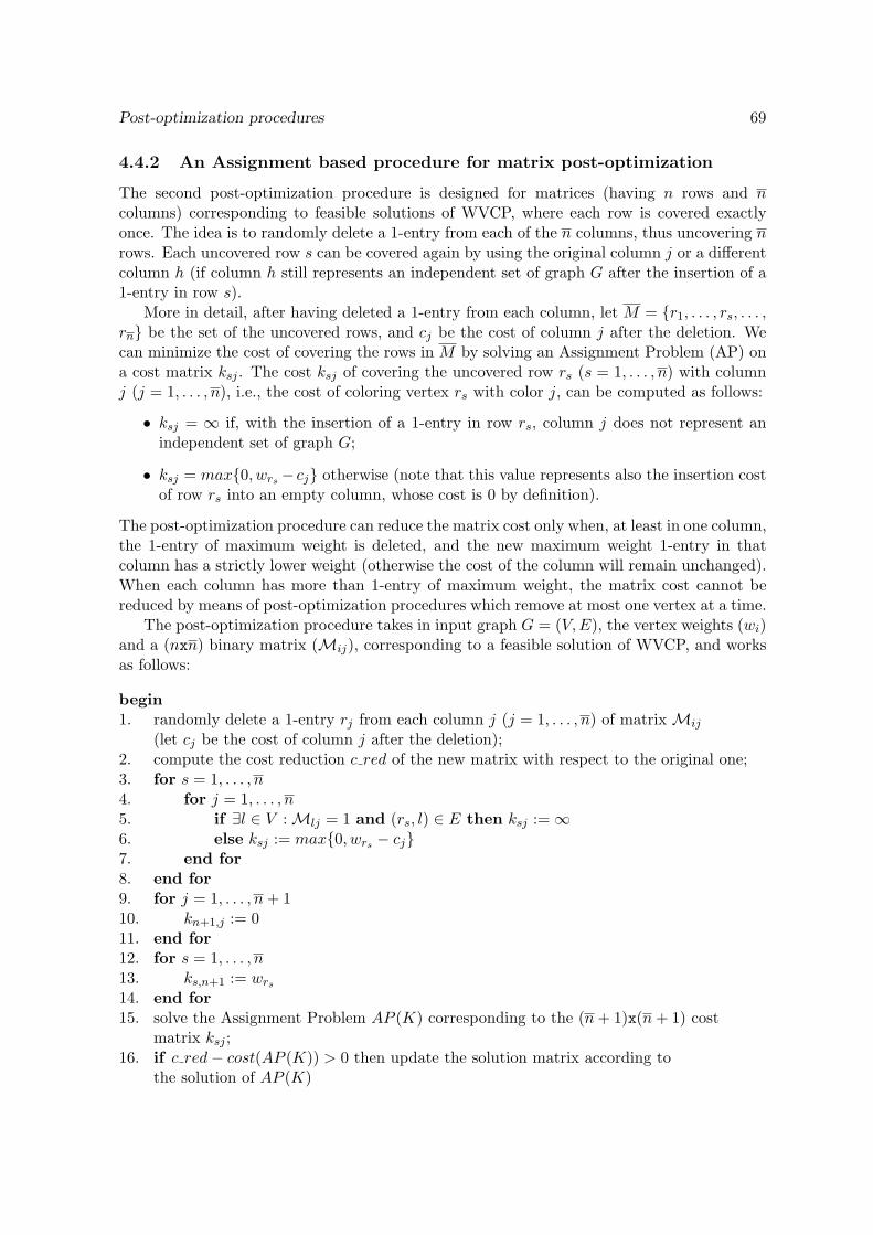
Post-optimization procedures 69
4.4.2 An Assignment based procedure for matrix post-optimization
The second post-optimization procedure is designed for matrices (having n rows and ncolumns) corresponding to feasible solutions of WVCP, where each row is covered exactlyonce. The idea is to randomly delete a 1-entry from each of the n columns, thus uncovering nrows. Each uncovered row s can be covered again by using the original column j or a differentcolumn h (if column h still represents an independent set of graph G after the insertion of a1-entry in row s).
More in detail, after having deleted a 1-entry from each column, let M = {r1, . . . , rs, . . . ,rn} be the set of the uncovered rows, and cj be the cost of column j after the deletion. Wecan minimize the cost of covering the rows in M by solving an Assignment Problem (AP) ona cost matrix ksj . The cost ksj of covering the uncovered row rs (s = 1, . . . , n) with columnj (j = 1, . . . , n), i.e., the cost of coloring vertex rs with color j, can be computed as follows:
• ksj = ∞ if, with the insertion of a 1-entry in row rs, column j does not represent anindependent set of graph G;
• ksj = max{0, wrs − cj} otherwise (note that this value represents also the insertion costof row rs into an empty column, whose cost is 0 by definition).
The post-optimization procedure can reduce the matrix cost only when, at least in one column,the 1-entry of maximum weight is deleted, and the new maximum weight 1-entry in thatcolumn has a strictly lower weight (otherwise the cost of the column will remain unchanged).When each column has more than 1-entry of maximum weight, the matrix cost cannot bereduced by means of post-optimization procedures which remove at most one vertex at a time.
The post-optimization procedure takes in input graph G = (V, E), the vertex weights (wi)and a (nxn) binary matrix (Mij), corresponding to a feasible solution of WVCP, and worksas follows:
begin1. randomly delete a 1-entry rj from each column j (j = 1, . . . , n) of matrix Mij
(let cj be the cost of column j after the deletion);2. compute the cost reduction c red of the new matrix with respect to the original one;3. for s = 1, . . . , n4. for j = 1, . . . , n5. if ∃l ∈ V : Mlj = 1 and (rs, l) ∈ E then ksj := ∞6. else ksj := max{0, wrs − cj}7. end for8. end for9. for j = 1, . . . , n + 110. kn+1,j := 011. end for12. for s = 1, . . . , n13. ks,n+1 := wrs
14. end for15. solve the Assignment Problem AP (K) corresponding to the (n + 1)x(n + 1) cost
matrix ksj ;16. if c red− cost(AP (K)) > 0 then update the solution matrix according to
the solution of AP (K)

70 Models and Algorithms for a Weighted Vertex Coloring Problem
end
On line 5 we set the cost ksj to ∞ when the assignment of row rs to column j cannot beperformed without violating any adjacency constraint on G (i.e., a constraint imposing thatthe columns must represent independent sets of G), otherwise we compute the correct coston line 6. We wish to allow a 1-entry to move to a new empty column having current cost 0,when this can reduce the global cost of the solution matrix, so we consider an AP associatedwith an (n + 1)x(n + 1) cost matrix where the last column of the cost matrix equals the rowweights (cost to be paid for the use of a new empty column) and the last row contains valuesequal to 0 (cost corresponding to the assignment of no 1-entry to a column, line 10). TheAP has always a trivial solution of value c red, consisting of the reassignment of the deleted1-entries to their original columns, but it can have better optimal solutions.
This post-optimization procedure can be used to improve all the greedy solutions generatedin Phase 1, where each row is covered exactly once. It can also be applied to the solutionmatrix found by Phase 2, after the application of the post-optimization procedure describedin Section 4.4.1.
4.5 Computational Analysis
The post-optimization procedures were coded in ANSI C and compiled with full optimizationoption; all the other procedures, including algorithm CFT [23], were coded in ANSI FOR-TRAN77 and compiled with full optimization option. The LP relaxation of the ILP modelM2 proposed in Section 4.2.2 was solved with CPLEX 9.0. The programs were run on a PIV2.4MHz with 512MB RAM under Windows XP.
We tested our codes on two different sets of instances: the first set was proposed during acomputational symposium on VCP and its generalizations [106], held in 2002, when weightswere added to vertices of the original DIMACS benchmark graph instances [73]. These in-stances correspond to different graph types and have been used for evaluating the performanceof VCP algorithms. In our experiments we considered all the random graphs (DSJCn.x), asubset of geometric random graphs (Geomn) (the smallest ones were disregarded) and all the“quasi-random” graphs (Rn x), where n denotes the number of vertices and x/10 is the den-sity of the graph. Our second set of instances is composed by problems from Traffic Matricesassociated to TDMA Traffic Assignment, proposed by Ribeiro, Minoux and Penna [99] andby Prais and Ribeiro [94], and available for download at [3].
All the computing times of the experiments reported in this Section are expressed inseconds of a PIV 2.4GHz. To allow a meaningful - although approximate - comparison ofthe computing times obtained on coloring problems with different machines, a benchmarkprogram (dfmax), together with a benchmark instance (r500.5), are available. Computingtimes obtained on different machines can be scaled w.r.t. the performance obtained on thisprogram (our machine spent 7 seconds “user time”).
4.5.1 Weighted Vertex Coloring Instances
In this Section we report the results obtained on 46 instances from [106]. No computationalexperience on these instances is reported in the literature.

Computational Analysis 71
In order to derive a lower bound on the optimal value of each instance, we solve theLP relaxation of ILP model M2 proposed in Section 4.2.2. We strengthen the model byreplacing the incompatibility constraints (4.9) between adjacent vertices with a set of cliqueconstraints (4.12), detecting cliques K ∈ K(h) in the following heuristic way: for each colorh and for each edge (i, j) such that i, j ≥ h, we compute a maximal clique K containingi, j and vertices having index larger or equal to h. This clique is initialized with vertices iand j, and then enlarged by iteratively adding new vertices, at each iteration considering theremaining vertices according to a non increasing degree ordering, and adding to the cliquethe first vertex which can fit (this simple greedy algorithm for the computation of a maximalclique is derived from the algorithm proposed by Johnson in [71]). The LP relaxation of theresulting model, involving O(n.m) clique constraints, was solved with CPLEX 9.0 by usingthe barrier algorithm with a time limit of 30 seconds. The choice of the barrier algorithm isdue to its performance on the set of instances considered, outperforming the primal and dualsimplex algorithms. For 44 instances over 46 (see above) the LP relaxation could be solvedwithin the time limit, providing a valid lower bound for the problem; for the remaining twoinstances, the LP relaxation was not solved to optimality within the time limit, hence nolower bound is available for these instances.
This lower bound LB, when successfully computed, is passed to the subsequent 2-phaseheuristic algorithm of Section 4.3, whose execution is stopped as soon as an incumbent solutionof value LB (i.e., an optimal solution) is found. All the results concerning the heuristicalgorithm are obtained by applying in sequence the ILP based post-optimization and theAssignment based post-optimization procedures to all the greedy solutions generated duringPhase 1, and to the final solution obtained by Phase 2. Due to the small size of the associatedproblems, the ILPs (4.17)-(4.20) can be solved to optimality within short computing timesby CPLEX 9.0. Since the solutions found by the Assignment based procedure depend on thevertices (rows) randomly deleted from the columns corresponding to the current solution, weapply, for 10 times, the procedure to all the solutions generated during the computation, afterthe ILP-based procedure, by increasing at every iteration the probability that the first vertexof each column is deleted. At the first iteration the Assignment based procedure takes ininput the output of the ILP-based procedure. The solution produced is then used as input forits next iteration, according to a local search paradigm. Considering the nj vertices coveredby a given column j according to non increasing weights, the probability pi of the i−th vertexto be deleted from column j is given by:
p1 = (iter + 1)/(iter + nj)(4.21)pi = 1/(iter + nj) for i = 2, . . . , nj(4.22)
where iter = 1, . . . , 10 represents the current iteration of the procedure. The AssignmentProblem is solved at every iteration by means of the Hungarian Algorithm, with the imple-mentation described by Carpaneto, Martello and Toth [28].
During Phase 1, several executions of each greedy algorithm are performed: at eachexecution, a small perturbation of the input ordering of the vertices is performed. Thealgorithm is able to generate different columns, and it is stopped as soon as 50 iterations areperformed without generating new columns. Our experiments showed that using a strongerperturbation of the input order would allow the algorithm to generate many more differentcolumns, but the quality of the final solution (i.e., the solution after phases 1 and 2) would beworse. The reason is that too many “bad” (i.e., not balanced) columns would be generated,

72 Models and Algorithms for a Weighted Vertex Coloring Problem
thus leading to large Set Covering instances, where it would be difficult, during Phase 2, tofind a good solution. This suggests that it is better to generate few good columns than a largenumber of columns of low quality. The perturbation is obtained by swapping two vertices inthe current ordering with a probability p = 40%. As for the completion of the columns to notdominated columns, the algorithm generates, from each column, two not dominated (possibly)different columns: the first one with no cost increase, the second one with a maximum costincrease ∆c, with ∆c = 1.5σ, where σ represents the standard deviation of the weights of thevertices of graph G.
Table 4.1 reports the computational results obtained by stopping Phase 1 after 500 iter-ations and Phase 2 after 75 seconds. For each instance, the following information are given:
• the instance name, number of vertices (n) and of edges (m);
• the lower bound (LB), corresponding to the rounded up solution value of the LP re-laxation described above, and the total time (TLB) required for the computation of thislower bound, including the heuristic generation of the maximal cliques for constraints(4.12) - for this reason the time limit of 30 seconds can be exceeded;
• the number of different columns (#col) generated during Phase 1;
• the best solution value found during Phase 1 (z1) and after Phase 2 (z2), respectively(the latter is reported only when improved with respect to the former);
• the computing time of Phase 1 (T1), corresponding to the column generation and thepost-optimization of every generated solution, and the computing time of Phase 2 (T2),including the post-optimization of the final solution;
• the improvements on the best solution values, obtained by applying the post-optimizationprocedures, with respect to the best solution values which can be obtained without thepost-optimization procedures, after Phase 1 (∆1), and at the end of the computation(∆2).
Finally, the last row of the table (∑
) reports the sum of the corresponding computingtimes.
The table shows that, over the 46 instances of our test bed, 12 can be solved to provenoptimality during Phase 1, confirming the effectiveness of the constructive heuristics proposedin Section 4.3.1 (optimal solutions are reported in bold). On the remaining 34 instances, thesecond phase of the algorithm was able to improve the incumbent solution 17 times, findinga proven optimal solution for 10 additional instances. In addition, we ran the ILP modelM2 with a very long time limit on the 24 instances for which optimality was not proven,finding that 6 additional solutions (marked with a ∗ in Table 4.1) are actually optimal, evenif the algorithm is not able to prove it. The post optimization procedures are quite effective,improving 8 times the incumbent solution after Phase 1 and 7 times the final solution afterthe two phases. E.g., for instance R50 9gb, ∆1 = 7 and ∆2 = 1 means that without the postoptimization procedures, the output of Phase 1 would have been 269 (instead of 262), andthat the output after Phase 2 would have been 263 (instead of 262). In other words, Phase2 would have improved the solution from 269 to 263, while the use of the post optimizationsleads to a solution of 262 after Phase 1, without further improvement on Phase 2. The onlyinstance for which the post-optimization procedures worsen the solution is DSJC125 5gb,

Computational Analysis 73
Table 4.1: Results on instances derived from DIMACS instances.Instance n m LB TLB #col z1 z2 T1 T2 ∆1 ∆2
DSJC125 1g 125 736 19 27 27471 24 82 70DSJC125 1gb 125 736 74 26 15381 95 100 70DSJC125 5g 125 3891 34 19540 76 110 70DSJC125 5gb 125 3891 35 14540 260 251 112 70 -1DSJC125 9g 125 6961 152 55 665 173 *169 157 5 1DSJC125 9gb 125 6961 568 42 744 628 605 167 70 5GEOM30b 30 111 12 6 12 12 0 0GEOM40b 40 197 16 0 166 16 1 0GEOM50b 50 299 18 0 26 18 0 0GEOM60b 60 426 23 0 52 23 0 0GEOM70 70 337 47 1 11502 48 47 96 0GEOM70a 70 529 73 0 1325 73 3 0GEOM70b 70 558 24 1 2459 24 6 0GEOM80 80 429 66 2 75 66 0 0GEOM80a 80 692 76 3 16232 78 76 100 2GEOM80b 80 743 27 3 24005 28 27 88 2GEOM90 90 531 61 3 18009 62 61 97 69GEOM90a 90 879 73 4 17094 75 73 101 56 1GEOM90b 90 950 30 5 5424 30 11 0GEOM100 100 647 65 4 20907 66 65 100 31GEOM100a 100 1092 89 7 23982 91 89 104 8GEOM100b 100 1150 32 7 7767 32 15 0GEOM110 110 748 66 7 23641 69 102 70GEOM110a 110 1317 97 12 25172 102 97 106 5 2GEOM110b 110 1366 37 19 3024 37 5 0GEOM120 120 893 72 8 32198 73 72 104 53 1GEOM120a 120 1554 105 10 34597 107 105 108 28GEOM120b 120 1611 35 28 9615 35 14 0 1
R50 1g 50 108 14 0 49 14 0 0R50 1gb 50 108 52 0 759 54 *53 94 1R50 5g 50 612 35 1 984 *37 97 70R50 5gb 50 612 126 1 922 137 75 70 1R50 9g 50 1092 73 1 134 *74 36 0 1R50 9gb 50 1092 257 1 148 *262 33 0 7 1R75 1g 70 251 17 4 10800 19 84 70R75 1gb 75 251 63 4 6509 72 96 70 1 1R75 5g 75 1407 43 6 4024 53 102 70R75 5gb 75 1407 160 6 3653 199 190 103 70 6R75 9g 75 2513 108 3 249 *110 79 0R75 9gb 75 2513 393 3 295 399 50 0 12 1R100 1g 100 509 18 13 19957 22 85 70R100 1gb 100 509 70 16 9135 84 101 70R100 5g 100 2456 48 28 11270 62 109 70R100 5gb 100 2456 182 32 9332 234 109 70R100 9g 100 4438 138 11 408 143 142 53 70R100 9gb 100 4438 499 11 501 529 520 120 7∑
490 3322 1458

74 Models and Algorithms for a Weighted Vertex Coloring Problem
where the final solution after Phase 2 is 251, while it could be 250 without the use of theprocedures. This can be explained by the different columns that are considered for the SetCovering instance, leading the heuristic search of algorithm CFT to a slightly worse solution.
4.5.2 Traffic Decomposition Matrix Instances
In this Section we report the results obtained on instances of the Matrix DecompositionProblem in TDMA Traffic Assignment.
These traffic matrices have to be decomposed into mode matrices (i.e., matrices whereno more than one non zero element is present in each row and column), in such a way thatthe sum of the costs of all the mode matrices is minimized, where the cost of each modematrix equals the maximum of its non zero elements. We can transform each instance of theproblem into a WVCP instance, by constructing the corresponding graph G, where every nonzero element corresponds to a vertex of the same weight and vertices in each row and columnare grouped into cliques of G. We take no advantage from the knowledge of the particularstructure of the corresponding graph, and apply the general 2-phase algorithm to these specialstructured graphs, with a proper tuning of the parameters.
Two subsets of instances were proposed in the literature: the p.n instances (having up to138 vertices and 1186 edges) that were solved to optimality by Ribeiro, Minoux and Penna[99], and heuristically by means of a GRASP algorithm by Prais and Ribeiro [94], and theR.n instances (having up to 301 vertices and 4122 edges) that were heuristically solved bymeans of the GRASP algorithm [94].
For each of the 35 p.n instances, Table 4.2 reports information similar to those givenin Table 4.1; in addition, the last two columns of the table give the solution value (zPR)found by Prais and Ribeiro [94] and the corresponding computing time (TPR) on a IBM9672 model R34 mainframe computer (note that instances p37 and p39 are missing from theinstance set). The results of Table 4.2 have been obtained without imposing a time limit inthe computation of the LP relaxation of model M2 (the corresponding computing time wasalways negligible), using no post optimization procedures, performing at most 50 iterationsof each greedy algorithm and stopping Phase 2 after a time limit of 1 second.
Further, we applied the Assignment based post optimization procedure, as explained inthe previous Section, to the two instances not solved to optimality, namely instances p13 andp42. The last two rows of Table 4.2 report the corresponding results. The optimal solutionof instance p13 was obtained by using the standard set up of the parameters for this setof instances, while the optimal solution of instance p42 was obtained by performing, duringPhase 1, 500 iterations of the greedy algorithms with a different perturbation of the vertices,and a longer time limit (6 sec.) in Phase 2, thus it is marked with a star ?.
The 2-phase Algorithm without the post-optimization procedures is able to find the op-timal solution on 33 over 35 instances, outperforming on this set of instances the approachproposed in [94], that finds the optimal solution on 31 instances over 35. The computingtimes are roughly comparable if we consider that our machine is from 40 to 60 times faster[42]. In addition, our approach is more general since it was not designed by considering thespecial structure of the p.n instances. When we add the Assignment based post-optimizationprocedure, the 2-phase Algorithm is able to find the optimal solution on 34 instances over 35,and on all the 35 with an ad hoc setting of the parameters for instance p42.
We also considered the 30 R.n instances, proposed in [94]. These instances have the samestructure as the p.n instances, but are larger. On these instances our approach does not

Computational Analysis 75
Table 4.2: Results on Traffic Decomposition Matrix Instances.Instance n m LB TLB #col z1 z2 T zPR TPR
p06 16 38 565 0.0 61 565 0.4 565 1.1p07 24 92 3771 0.0 79 3771 0.1 3771 4.0p08 24 92 4049 0.0 179 4074 4049 1.3 4049 1.3p09 25 100 3388 0.0 36 3388 0.1 3388 3.0p10 16 32 3983 0.0 0 3983 0.1 3983 4.5p11 18 48 3380 0.0 0 3380 0.1 3380 4.7p12 26 90 657 0.0 0 657 0.1 657 3.8p13 34 160 3220 0.1 673 3255 3225 2.3 3230 7.8p14 31 110 3157 0.0 85 3157 0.1 3157 10.1p15 34 136 341 0.1 101 341 0.1 341 4.7p16 34 134 2343 0.1 414 2343 0.5 2343 14.5p17 37 161 3281 0.1 876 3334 3281 1.4 3281 5.5p18 35 143 3228 0.1 160 3228 0.2 3228 10.4p19 36 156 3710 0.1 0 3710 0.1 3710 14.6p20 37 142 1830 0.1 914 1860 1830 1.3 1860 20.0p21 38 155 3660 0.1 164 3660 0.2 3660 18.4p22 38 154 1912 0.1 232 1912 0.2 1912 20.0p23 44 204 3770 0.1 1357 3790 3770 1.4 3810 21.4p24 34 104 661 0.1 0 661 0.1 661 27.9p25 36 120 504 0.1 0 504 0.1 504 23.9p26 37 131 520 0.1 0 520 0.1 520 28.3p27 44 174 216 0.1 259 216 0.2 216 7.8p28 44 164 1729 0.1 0 1729 0.1 1729 44.5p29 53 254 3470 0.1 0 3470 0.1 3470 65.7p30 60 317 4891 0.2 2594 4902 4891 2.1 4891 56.6p31 47 179 620 0.1 0 620 0.1 620 70.9p32 51 211 2480 0.1 0 2480 0.0 2480 70.9p33 56 258 3018 0.2 0 3018 0.1 3018 62.3p34 74 421 1980 0.3 171 1980 0.1 1980 131.9p35 86 566 2140 0.5 183 2140 0.1 2140 135.0p36 101 798 7210 0.9 48 7210 0.1 7210 163.1p38 94 537 2130 0.6 972 2130 0.4 2130 70.5p40 86 497 4879 0.5 439 4984 0.2 4984 224.2p41 116 900 2688 1.3 351 2688 0.1 2688 313.7p42 138 1186 2466 2.1 5314 2509 2.8 2480 405.8
p13.col 34 160 3220 0.1 664 3255 3220 8.7 3230 7.8?p42.col 138 1186 2466 2.1 20191 2503 2466 99.8 2480 405.8

76 Models and Algorithms for a Weighted Vertex Coloring Problem
work well, because too many columns must be generated during Phase 1 in order to set upa “good” subfamily S ′. In addition, Phase 2 is able to improve on the best greedy solutionsonly in 3 cases over 30 (the Assignment based post-optimization procedure being used). Sowe were able to find (in comparable computing times) only 3 times a solution better thanthe one reported in [94] (and two of these improvements correspond to the instances wherePhase 2 is effective), 9 times a solution of the same value and in the remaining 18 cases aworse solution.
4.6 Conclusions
This paper presents 3 ILP models and a 2-phase heuristic algorithm for a Weighted VertexColoring Problem, for which there is theoretical interest but lack of computational work. Inparticular, the second model is aimed at breaking symmetries appearing into classical VCPmodels, and its continuous relaxation yields a good lower bound on the optimal solution of theproblem. The heuristic algorithm is based on the Set Covering formulation of the problem, inwhich variables correspond to independent sets. In the first phase a large number of feasiblesolutions is generated by means of fast greedy heuristics designed for the problem; everygenerated solution can be improved by using two post optimization procedures, the first basedon the optimal solution of an ILP model, the second on the solution of an Assignment Problem.In the second phase an associated set-covering instance is solved by using a Lagrangian-basedheuristic algorithm from the literature.
Extensive computational results on two sets of instances from the literature are reported,the first set being composed of general graphs and the second set of graphs obtained fromTraffic Matrices from TDMA Traffic Assignment. The reported computational experimentsshow the effectiveness of the approach, where each component of the Algorithm is able toimprove the best incumbent solution, and the lower bound is able to prove the optimality ofmany solutions. On a class of the second set of instances, the 2-phase algorithm outperformsa specialized algorithm, that was specifically designed by considering the particular structureof the instances.
The two main contributions of this paper are represented by the definition of model M2and by the two post optimization procedures. In particular, these procedures, as well as theoverall 2-phase approach, can be applied to combinatorial optimization problems that can beformulated as a Set Covering Problem, and where the costs have the special structure of theconsidered problem, see e.g. the Level Strip Packing Problem with Shelves (Lodi, Martelloand Vigo [83]).
In future work, we plan to better explore the properties of model M2, and to implementthe LP relaxation of the Set Covering model M3 in a column generation framework, in order todesign effective exact algorithms. In addition, we would like to apply the 2-phase algorithmto different problems with a Set Covering formulation and the same cost structure of thecolumns. It would be also interesting to solve the second phase (column optimization) byusing a different approach to the Set Covering Problem, in order to improve the results onsome instances where the Lagrangian heuristic algorithm we have used has a not satisfactoryperformance.

Chapter 5
Lower and Upper Bounds for theBounded Vertex Coloring Problem
1
We address a particular Vertex Coloring Problem, where each vertex i has associated apositive weight wi, and the sum of the weights of the vertices assigned to the same color cannotexceed a given capacity C. The problem, known as the Bounded Vertex Coloring Problemor Bin Packing Problem with Conflicts, is of practical and theoretical interest, because of itsmany real-world applications and because it generalizes both the Bin Packing Problem andthe Vertex Coloring Problem. We present new lower and upper bounds and investigate theirbehavior by means of computational results on benchmark instances.
5.1 Introduction
This paper considers a Bounded Vertex Coloring Problem, where, given a graph G = (V, E),each vertex i has associated a positive weight wi. As in VCP, one is required to assign acolor to each vertex in such a way that adjacent vertices have different colors, and the totalnumber of colors is minimized. The problem asks to satisfy an additional constraint: thetotal capacity of colors is bounded, i.e. the sum of the weights of the vertices assigned to thesame color cannot exceed a given capacity C, which is the same for all colors.
The same problem can be interpreted as a Bin Packing Problem with Conflicts (BPPC),in which we are given n items i with weight wi and an infinite number of identical bins ofcapacity c. Two items i and j are said to be conflicting if and only if they cannot be assignedto the same bin. The aim of the problem is to assign all items in the minimum number of bins,while ensuring that the total weight of all items assigned to a bin does not exceed the weightcapacity and that no bin contains conflicting items. Since in the following we will use andextend some results from the Bin Packing literature, we will use the Bin Packing terminology,thus considering ”items and bins”, and V will be the set of items. However, this terms areperfectly interchangeable with ”vertices and colors”, if the reader is more comfortable in aVCP setting.
Thus, the problem we tackle is a BPP with incompatibilities described by a conflictinggraph G = (V,E), where each item corresponds to a vertex, and two vertices are connected
1Preliminary results of this chapter appear in [47].
77

78 Lower and Upper Bounds for the Bounded Vertex Coloring Problem
by an edge when the corresponding items are pairwise incompatible. Note that this graphdoes describe the incompatibilities due to the capacity constraints. In other words, if twoitems, when considered together, exceed the bin capacity, there is not necessarily an edgeconnecting them in G. In addition to graph G, we consider graph G′ = (V, E′), with E′ =E ∪ {(i, j) ∈ E : wi + wj > C}. Incompatibility graph G′ describes all the incompatibilitiesof the problem.
This problem generalizes both the classical VCP, which is a special case of BPPC wherewj = 0 for j = 1, . . . , n; as well as the Bin Packing Problem (BPP, see Martello and Toth[88]), which is a special case of the BPPC where no item is in conflict with another item, i.e.,E = ∅;
Some well-known applications of the problem concern examination scheduling (see, La-porte and Desroches [78]), the assignment of processes to processors and the load balancingof tasks in parallel computing (see Jansen [66]), and particular delivery problems where somesubstances cannot be placed in the same vehicle (see Christofides, Mingozzi and Toth [31]).A similar problem, where a number of conflicting examinations have to be scheduled in thesmallest number of periods, under capacity restrictions, was considered by Carter, Laporteand Lee in [29], where greedy heuristics are reported.
The Bounded Vertex Coloring Problem with all weights equal to 1 was considered byHansen, Hertz and Kuplinsky in [60], where upper and lower bounds, as well as complexityresults are given. Jansen and Oehring [67] and Jansen [66] have shown that, for general graph,no polynomial time approximation schemes can be derived, while they derive polynomial timeapproximation schemes for special classes of graphs. Baker and Coffman [11] derived similarresults for the problem where vertices weights can be larger that one, while Bodlaender andJansen [17] considered the complexity of the problem for different conflict graph classes.
The most relevant computational work on BPPC was provided by Gendreau, Laporte andSemet [55]. In [55] the authors survey the previous results in the literature of the BPPC,present new lower and upper bounds and introduce benchmark instances used to test thebehavior of the algorithms.
This paper is aimed at providing new lower and upper bounds for the BPPC and to providetheir efficacy be extensive computational results. In Section 5.3 we survey lower bounds fromthe literature and introduce new ones. In Section 5.4 we present several upper bounds, bothnew and from the literature, and adapt to the BPPC the metaheuristic developed for theVCP by Malaguti, Monaci and Toth [84]. In Section 5.5 we give the computational resultsobtained.
5.2 ILP model
The BPPC can be modelled (see Gendreau, Laporte and Semet [55]) by introducing thefollowing variables:
yh =
{1 if bin h is used0 otherwise
(5.1)
for h = 1, . . . , n, and
xih =
{1 if item i is assigned to bin h0 otherwise
(5.2)

Lower Bounds 79
for i = 1, . . . , n, h = 1, . . . , n. We obtain the following model:
minn∑
h=1
yh(5.3)
n∑
h=1
xih = 1 i = 1, . . . , n(5.4)
n∑
i=1
wixih ≤ Cyh h = 1, . . . , n(5.5)
xih + xjh ≤ 1 ∀(i, j) ∈ E, h = 1, . . . , n(5.6)yh ∈ {0, 1} h = 1, . . . , n(5.7)
xih ∈ {0, 1} i = 1, . . . , n, h = 1, . . . , n(5.8)
Objective function (5.3) minimized the number of bins (resp. colors) used. Constraints(5.4) require that each item is assigned to a bin (resp., each vertex is colored). Constraint(5.5) are the classical capacity constraints of Bin Packing, while (5.6) are the classical in-compatibility constraints of VCP, which are here reported as edge constraints, but can bestrengthened to clique constraints, like discussed, e.g., in [85]. Finally, (5.7) and (5.8) imposethe integrality of used variables.
5.3 Lower Bounds
We first note that any lower bound for the BPP is a valid lower bound also for BPPC.Analogously, any lower bound for the VCP is also a lower bound for the BPPC. We thusimplemented the following procedures derived from the BPP literature:
• L0BPP : continuous lower bound for the BPP, computed as the rounding up of the sum
of the weights divided by the bin capacity:
L0BPP = d
n∑
i=1
wi/Ce(5.9)
• L1BPP : improved bound on the BPP, denoted as L2 in Martello and Toth [88], based on
the partitioning of items into sets according to weight thresholds: given 0 < α < C/2and I1 = {i : wi > C − α}, I2 = {i : C/2 < wi ≤ C − α}, I3 = {i : α < wi ≤ C/2},
L1BPP = |I1|+ |I2|+ max(0, d
∑i∈I3 wi − (C|I2| −
∑i∈I2 wi)
Ce)(5.10)
In addition, since the problem is a generalization of the VCP, we implemented the followinglower bound based on the computation of a maximal clique:

80 Lower and Upper Bounds for the Bounded Vertex Coloring Problem
• LMC : compute a maximal clique on the incompatibility graph G = (V, E) through thegreedy heuristic of Johnson [71]. Initialize the clique with the vertex i of maximumcardinality. Then enlarge it by iteratively adding new vertices, at each iteration consid-ering remaining vertices according to a non increasing degree ordering, and adding tothe clique the first which can fit. In [55] Gendreau et al. propose to compute the cliqueon graph G′ instead of graph G. Even if any maximum clique of G is by constructionincluded in a maximum clique of G′, computing a maximal clique of G′ by means ofthe Johnson’s algorithm can result in disappointing results. Actually, the drawback ofthis strategy is that vertices of high weight result systematically in high degree vertices,even when they are not included in large cliques of G′.
We propose the following improvement to the computation of LMC , and call it L′MC :compute a maximal clique K on G by means of Johnson’s algorithm, and then add toE all edges (i, j) such that wi + wj > C, thus obtaining graph G′. Then, expand Kto K ′, which is a maximal clique of G′. By construction, cardinality of K ′ is larger orequal than cardinality of K, and, on average, (see Section 5.5), this strategy leads tolarger cliques than the use of Johnson’s algorithm directly on graph G′.
Now let us consider a lower bound explicitly developed for the BPPC.
• The constrained packing lower bound (LCP ) was introduced by Gendreau, Laporte andSemet in [55]. A maximal clique of graph G′ is computed by means of Johnson’salgorithm. A bin is used for each of the clique vertices, and then items that can fitin these bins are inserted, possibly in a fractional way, but by satisfying compatibilityconstraints (this requires the solution of a transportation problem, see [55] for furtherdetails). All items (integer or fractional) than can not fit in the clique bins are storedin a different set N2, on which a continuous relaxation based bound L0
BPP is computed.A valid lower bound for the problem is then LBCP = |K|+ L0
BPP (N2).
We improved this bound in the maximal clique computation, computing L′MC insteadof LMC , and obtaining bound L′CP .
In the next Sections we present new lower bounds for the BPPC.
5.3.1 A surrogate relaxation
Let us consider model (5.3)–(5.8). We first note that constraints (5.6) can be lifted in thefollowing way:
xih + xjh ≤ yh ∀(i, j) ∈ E, h = 1, . . . , n(5.11)
since if bin h is not used, then both variables take value 0. We now study a possiblesurrogate relaxation of constraints (5.11). We sum the original n|E| constraints over theedges, with all multipliers equal to 1, and we obtain the following n constraints, where δi
denotes the degree of vertex i:

Lower Bounds 81
n∑
i=1
δixih ≤ |E|yh ∀h = 1, . . . , n(5.12)
Now note that model (5.3), (5.4), (5.5), (5.12), (5.7) and (5.8) represents what is knownin the literature as Two-Vector Packing Problem (TVPP), which is a generalization of theBPP in which two dimensions and two capacity constraints are present. The TVPP is NP-complete, and was solved to optimality, with Branch and Bound techniques by Spieksma[104]. However, it is not our objective to solve it to optimality, but refer to lower boundsfrom the literature. We thus obtain the following procedure:
• LTV PP : relax in a surrogate way the constraints of the BPPC so as to obtain a TVPP.Apply procedure Lc defined in Caprara and Toth [24] to the TVPP instance obtainedso as to get to a valid BPPC lower bound.
5.3.2 A Lower Bound based on Matching
Consider an instance of BPPC with 5 items, having the following weights: {1, 1, 5, 5, 5}, andbins of capacity 10. The only edge of the incompatibility graph G′ connects the two items ofweight 1. For this instance, L0
BPP = L1BPP = LBCP = LB′
CP = LTV PP = 2, when clearly3 bins are needed. Actually this is a set of items that are pairwise compatible (with theexception of the two items of weight 1), but no subset of cardinality tree of the items can fitin one bin. We say that these items are incompatible 3 by 3. In general, given a set S ofitems with the property that at most two of them can fit in one bin, the best way to solvethe corresponding BPPC is actually to match as many items as possible, by satisfying theincompatibilities of graph G′, and use 1 bin for all matched pairs, and 1 bin for items thatcould not be matched. In other words, we can compute a valid lower bound as the cardinalityof a maximum cardinality matching M on the complement graph G′ of G′, plus the numberof unmatched items, as follows:
Lmatch = |M |+ (|S| − 2|M |) = |S| − |M |(5.13)
The computation of the set S, which is in general a subset of the n items, having theproperty that its elements are incompatible 3 by 3, is far from trivial. We want the set Sto be inclusion maximal, i.e. such that, ∀ item j /∈ S, the property does not hold for j ∪ S.In addition, we may want S to be the maximum cardinality set of items incompatible 3 by3. The computation of the maximum cardinality set with the desired property, on a generalgraph, is NP-hard, and however there is not guarantee that the maximum cardinality set Swould lead to the largest value of the bound Lmatch, which depends on the cardinality of thematching.
Thus, we compute set S by combining items of large weight and items which are includedin a maximal clique K in a greedy way. We define a parameter β such that 0 ≤ β ≤ 1/2C andit exists at least one item having weight β, and for each value of β we compute a correspondingset Sβ. Then, we compute the lower bound Lmatch for each Sβ and we keep the largest:
1. Lmatch = 0;

82 Lower and Upper Bounds for the Bounded Vertex Coloring Problem
2. order items i according to not increasing weight;3. for each β such that: ∃i : wi = β, 0 ≤ β ≤ 1/24. Sβ := {i ∈ K, wi ≥ β};5. for i = 1, . . . , n, i /∈ Sβ
6. if Sβ is a set of items incompatible 3 by 3 after the insertion of i7. Sβ := Sβ ∪ {i}.8. end for9. if Lmatch < |Sβ| − |Mβ|10. Lmatch := |Sβ| − |Mβ|;11. end for
5.4 Upper Bounds
We first adapt to the BPPC heuristic algorithms originally proposed for the BPP. Let usorder the items according to non-increasing weight. We obtain:
• First-Fit Decreasing with Conflicts (FFC), adaptation of the FFD algorithm for BinPacking: consider each item in turn and assign it to the first bin in which there issufficient residual capacity and for which there is no conflict with the already assigneditems;
• Best-Fit Decreasing with Conflicts (BFC): as in FFDC, but the items is assigned to thebin for which there is enough residual capacity, no conflicts, and for which the resultingtotal sum of the weight is maximum;
• Worst-Fit Decreasing with Conflicts (WFC): as in BFDC, but resulting total sum ofthe weight must be minimum.
Obviously the previous algorithms are direct adaptation to the BPPC of the well-knownheuristics by Johnson [70] (see also Coffman, Garey and Johnson [33] for heuristic algorithmsfor the BPP). Let us define FD as the best solution value found by the previous three algo-rithms.
An improved class of heuristics can be obtained by considering the following surrogateweight:
wsi = α
wi
C+ (1− α)
δi
|E|(5.14)
for i = 1, . . . , n, with 0 ≤ α ≤ 1 and δi is equal to the number of incident edges in G′ (i.e., thenumber of incompatibilities of i). Now we can order the items according to non-increasingws
i and execute the three previous heuristics. According to computational evidence we setα = 0, 0.1, . . . , 1, running 11 times each heuristic. Let us define FFC-α, BFC-α, WFC-α thesolutions obtained by running respectively FFC, BFC and WFC. Let us also define FD-α asthe best solution among these three.
So far we implemented six different heuristics. We finally include in the list the heuristicH6, which is the best among the upper bounds proposed by Gendreau, Laporte and Semet[55].

Upper Bounds 83
We refer to Section 5.5 for the computational results obtained by these heuristics. If thesolution found is not equal to the lower bound of the previous section, then it is possiblyimproved by means of the following metaheuristic procedure.
5.4.1 Evolutionary Algorithm
To find high quality solutions on difficult instances, we use a variation of the metaheuristicEvolutionary Algorithm described in [84], which combines an effective tabu search with aspecialized diversification strategy.
Tabu Search Algorithm
In [84] a Tabu Search procedure is proposed which moves between partial feasible solutions,i.e., in a VCP framework, colorings where all incompatibility and capacity constraints aresatisfied, but not all vertices are colored, or, with regards to a BPPC framework, solutionsin which each bin satisfies capacity and incompatibility constraints, but not all items areassigned to a bin. We modify this procedure in order to solve the BPPC. In [92] Morgensterndefines the Impasse Class Neighborhood, a structure used to improve a partial solution of costk to a complete solution of the same value. The Impasse Class requires a target value k forthe number of bins (resp. colors in the VCP) to be used. A solution S is a partition of Vin k + 1 bins {V1, ..., Vk, Vk+1} in which all bins, but possibly the last one, are feasible bins.This means that the first k bins constitute what we define as a partial feasible k partitioning,while all items that do not fit in the first k bins are in the last one. Making this last binempty gives a complete feasible k partitioning. To move from a solution S to a new solutionS′ ∈ N(S) one can randomly choose an unassigned item i ∈ Vk+1, assign i to a different bin,say h, and move to bin k +1 all items j in bin h that are incompatible to i. This assures thatbin h remains feasible with respect to incompatibility constraints. If the capacity constraintis not satisfied, extra items have to be moved from bin h to k + 1, till the capacity of bin his exceeded. We considered four possibilities:
• move items according to decreasing weight ordering;
• move items according to increasing weight ordering;
• move items according to a random ordering;
• move items by minimizing the score (defined below) of moved items. If B is the actualbin weight and C the capacity, we want to select a subset of the items in bin h, tobe moved to bin k + 1, such that the sum of the corresponding scores is minimizedand the total weight is larger than B − C. This is equivalent to maximize the sum ofthe scores of items that are kept in h, without exceeding the bin capacity, i.e. it is aKnapsack Problem or a Subset Sum Problem if the score of each item equals its weight(see Martello and Toth [88]).
The Class h is chosen by comparing different target classes by means of a function f(S)for evaluating the corresponding solutions S. Rather than simply minimizing | Vk+1 | it seemsa better idea to minimize the value:
f(S) =∑
j∈Vk+1
δj(5.15)

84 Lower and Upper Bounds for the Bounded Vertex Coloring Problem
if we want to give more importance to the compatibility constraints, and
f(S) =∑
j∈Vk+1
wj(5.16)
if we want to give more importance to the capacity constraints. Moreover, we can use thesurrogate weight ws
j to combine weight and degree of the vertices:
f(S) =∑
j∈Vk+1
wsj(5.17)
At every iteration we move from a solution S to the best solution S′ ∈ N(S) (even iff(S) < f(S′)). To avoid cycling, we use the following tabu rule: an item i cannot enter thesame bin h it entered during one of the last T iterations; for this purpose we store in a tabulist the pair (i, h). While pair (i, h) remains in the tabu list, item i cannot be assigned to binh. We also use an Aspiration Criterion: a tabu move can be performed if it improves on thebest solution encountered so far. To summarize, the Tabu Search algorithm takes in input:
• graph G(V, E);
• the weights of the items and the bin capacity C;
• the target value k for the number of bins;
• a feasible partial k partitioning;
• the maximum number L of iterations to be performed ;
• the tabu tenure T .
If the algorithm solves the problem within L iterations it gives on output a feasible solutionof value k, otherwise it gives on output the best scored infeasible solution found during thesearch.
The Tabu Search algorithm is very simple and requires as parameter to be experimentallytuned only the tabu tenure T . At the same time it has a good experimental behavior, sinceit is often able to find good solutions in very short computing times. The main drawbackof this approach is that it seems unable to efficiently explore the whole solution space, thussuggesting the integrations of the Tabu Search with a suitable diversification strategy.
Evolutionary Diversification
To improve its performance, the Tabu Search can be used together with a diversificationoperator, as in the Evolutionary algorithm proposed in [84].
In our algorithm we start with an initial pool of partial feasible solutions of value k (inthe following simply solutions) obtained by using the Tabu Search procedure initialized withdifferent random seeds. Then we apply the Tabu Search algorithm to improve these solutionsduring the local search phase. We use a crossover operator similar to the one used in [84],which is a variation of the specialized crossover operator Greedy Partition Crossover proposedby Galinier and Hao [51] for Vertex Coloring Problems. Our purpose is to extend a feasiblepartial k partitioning to a complete partitioning. The general procedure is summarized asfollows: given a pool of solutions, we randomly choose two parents from the pool and generate

Upper Bounds 85
an offspring, which is improved by means of the Tabu Search algorithm and finally insertedin the pool, deleting the worst parent. After the initialization, the generation-improvement-insertion procedure is iterated until the problem is solved (i.e. a partial feasible solution isextended to a complete solution) or a time limit is reached.
The crossover operator has the same structure as the one described in [84] for the classicalVCP: given two parents S1 = {V 1
1 , ..., V 1k , V 1
k+1} and S2 = {V 21 , ..., V 2
k , V 2k+1} the crossover
operator outputs the offspring S3 = {V 31 , ..., V 3
k , V 3k+1} by considering iteratively parent S1
and S2, picking up the bin maximizing a given score in the actual parent, copying it tothe offspring, and deleting items contained in the chosen bin from both parents. The onlydifference concerning the operator is that we consider different possible scores, when pickingup the next bin to be copied to the offspring:
• the cardinality of the bin;
• the total weight of the bin;
• the sum of the degrees of the items in the bin;
• the total surrogate weight of the bin.
Solution evaluation
The quality (fitness) of every solution S in the pool is evaluated through the function f(S)defined by (5.15) or (5.16) or (5.17) and used during the Tabu Search algorithm. This allowsus to compare the solutions and to tune the quality of the pool during the computation. Theoffspring is then inserted in the pool, substituting the worst parent.
Parameter Setting
The Evolutionary Algorithm uses different parameters, whose set-up is important in orderto obtain good quality solutions. Moreover, the strategy adopted when emptying bins, in orderto satisfy the capacity constraints, the solutions evaluating function and the score functionused by the crossover operator must be specified. Our experiments on the set of instancesproposed by Gendreau et al. [55] suggested to consider two different kind of instances: lowdensity instances (with graph density up to 0.3) and hight density instances (with graphdensity larger than 0.3). For low density instances, we set L = 5000, poolsize = 10, T = 90and we use the solution evaluating function (5.16). For high density instances, we set L =5000, poolsize = 10, T = 60 and we use the solution evaluating function (5.15). In bothcases, when emptying a bin, we consider items in a random ordering and we remove them tillthe bin exceeds the capacity. This introduces more randomness in the algorithm than otherstrategies, and leads to better results on the considered instances. We initialize the algorithmwith a dummy solution (all bins are empty) and a very large number of bins available. Wecompute then the actual number of used bins, say k, and we iterate reducing k to k − 1until the algorithm in able to solve the problem within a given time limit, which is set to 50seconds. In the crossover operator, we use as score for the bin to be copied from the parentto the offspring, the cardinality of the bin.

86 Lower and Upper Bounds for the Bounded Vertex Coloring Problem
5.5 Computational Experiments
The algorithms were coded in C and run on a Pentium IV 3 GHz. Their behavior was testedon the instances proposed by Gendreau, Laporte and Semet [55]. They considered 8 classesof instances from Falkenauer [46], each class containing 10 bin packing instances. By adding,for the instances of each class, random incompatibility graphs G, with densities varying from0 to 0.9, they obtained 800 instances (100 for each class). We refer the reader to the originalpublication for more details.
The results of the upper bounds are summarized in Tables 5.1 and 5.2, where Ev. standsfor the metaheuristic of Subsection 5.4.1. In each column we report the average value foundby each algorithm on the ten instances of each class, for different values of the density dens.of the associated graph G. It can be seen as Ev., whose computing times are comparable withthose of GLS6, clearly outperforms previous techniques.
The results of the lower bounds are summarized in Tables 5.3 and 5.4. We report resultson the bounding procedures presented on this paper, with the exception of LTV PP and Lmatch,for which the interest is only theoretical since they have a non satisfactory performance fromthe computational viewpoint. L1
BPP , by definition, cannot perform worse than L0BPP , hence
the results of the latter are not reported. Also in this case we can see that there is a lowerbound that clearly outperforms the others, namely L1
BPPC .Finally in Table 5.5 we compare upper and lower bounds. In the table, #opt stands for
the number of proven optimal solutions, and %gap to the percentage gap between lower andupper bound. 487 instances over 800 were solved to optimality, with a very small percentagegap between lower and upper bound, being 0.5% on average.
5.6 Conclusions
We considered a bounded version of the Vertex Coloring Problem (BVCP), combining bothVCP and the Bin Packing Problem. We report lower bounds from the VCP and BPP lit-erature, which are valid for the considered problem as well, we improve a lower bound fromthe literature and present new lower bounds, exploiting the double nature of the problem.Similarly, we report from the literature upper bounds for the BVCP problem, we proposenew heuristic upper bounds adapted from the BPP literature, and we adapt an effectivemetaheuristic approach, proposed for VCP, to the problem.
We implemented and compared original and literature algorithm on a set of 800 instancesfrom a benchmark set. By using a combination of heuristic and metaheuristic approaches,we are able to solve to proven optimality 383 out of 800 instances, while previous approachescould solve to optimality only 179 out of 800, with comparable computational effort.

Conclusions 87
Table 5.1: Upper bounds results for classes 1–4.Class dens. FFC BFC WFC FFCα BFCα WFCα H6 Ev. min
1 0 49.1 49.1 49.5 49.1 49.1 49.5 49.4 48.3 48.31 49.3 49.3 49.6 49.1 49.1 49.3 49.7 48.3 48.32 51.1 51.1 51.0 49.1 49.1 49.7 50.4 48.3 48.33 55.4 55.7 54.6 49.3 49.3 50.3 50.6 48.5 48.54 63.2 63.4 59.4 53.5 53.6 54.1 54.9 53.0 53.05 72.8 72.8 69.5 64.6 65.1 64.6 65.3 64.3 64.36 83.0 83.1 79.8 76.0 76.5 76.3 76.9 75.8 75.87 93.2 93.5 91.1 87.8 88.1 88.0 87.9 87.5 87.58 102.2 102.3 100.4 98.5 98.6 98.5 99.0 98.3 98.39 110.9 110.9 110.6 109.8 109.8 109.8 110.0 109.8 109.8
2 0 102.9 102.9 103.2 102.9 102.9 103.2 103.8 101.7 101.71 103.6 103.6 103.4 103.0 102.9 103.1 104.0 101.7 101.72 105.6 105.6 105.0 103.0 103.0 103.8 105.1 101.7 101.73 114.3 114.5 110.4 103.4 103.2 104.7 106.1 101.7 101.74 129.6 130.2 119.7 106.4 106.2 108.3 109.4 105.3 105.35 148.1 148.3 138.0 126.7 127.5 127.5 129.2 126.0 126.06 168.2 168.6 162.1 153.0 153.4 153.6 154.3 152.3 152.37 188.1 188.5 184.5 177.4 178.3 178.1 179.2 177.1 177.18 209.2 209.4 207.4 202.8 203.2 203.1 203.9 202.7 202.79 230.3 230.3 229.2 226.8 227.0 227.2 227.9 226.8 226.8
3 0 205.3 205.3 205.7 205.3 205.3 205.7 206.5 204.0 204.01 205.9 206.0 205.9 205.4 205.4 205.6 207.8 204.0 204.02 211.2 211.4 210.0 205.7 205.4 206.9 209.4 203.9 203.93 225.6 226.7 222.8 206.1 205.7 210.1 211.4 203.8 203.84 256.3 256.8 241.5 211.7 212.3 216.1 216.4 212.1 210.85 294.2 295.0 275.4 254.1 255.0 255.5 257.6 252.5 252.56 335.6 336.3 320.4 305.2 306.0 305.2 307.1 304.1 304.17 374.6 374.9 363.8 351.8 352.5 352.9 354.2 350.4 350.48 416.7 416.9 409.9 399.9 400.4 400.6 402.2 399.1 399.19 460.8 460.9 458.4 452.8 453.0 453.5 454.0 452.4 452.4
4 0 406.7 406.7 407.1 406.7 406.7 407.1 408.4 406.5 406.21 407.4 407.5 407.6 406.5 406.5 407.1 411.1 406.3 406.12 418.2 418.7 414.3 407.1 407.0 409.6 413.6 405.7 405.73 444.6 446.4 441.0 407.7 407.6 416.8 416.0 405.5 405.54 498.9 501.0 475.1 415.6 416.8 424.3 424.4 423.8 414.95 579.8 580.8 543.3 509.3 511.0 510.8 513.3 505.3 505.36 665.9 666.9 637.5 610.0 611.8 610.8 613.2 607.5 607.57 752.5 753.0 731.3 710.2 710.9 710.9 712.9 707.6 707.68 837.8 838.5 825.1 808.5 809.6 809.7 810.3 807.3 807.39 922.3 922.4 916.2 906.4 906.8 907.2 908.1 905.7 905.7
Average 278.8 279.1 272.3 262.0 262.3 263.2 264.4 261.2 260.9
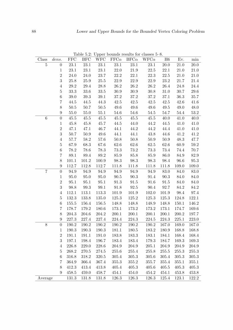
88 Lower and Upper Bounds for the Bounded Vertex Coloring Problem
Table 5.2: Upper bounds results for classes 5–8.Class dens. FFC BFC WFC FFCα BFCα WFCα H6 Ev. min
5 0 23.1 23.1 23.1 23.1 23.1 23.1 20.0 21.0 20.01 23.1 23.1 23.1 22.0 21.9 22.5 22.1 21.0 21.02 24.0 24.0 23.7 22.2 22.1 22.3 22.5 21.0 21.03 25.8 25.9 25.5 22.9 22.9 22.9 23.2 21.7 21.44 29.2 29.4 28.8 26.2 26.2 26.2 26.4 24.8 24.45 33.3 33.6 33.5 30.9 30.9 30.8 31.0 30.7 29.66 39.0 39.3 39.1 37.2 37.2 37.2 37.1 36.3 35.77 44.5 44.5 44.3 42.5 42.5 42.5 42.5 42.6 41.68 50.5 50.7 50.5 49.6 49.6 49.6 49.5 49.0 48.09 55.0 55.0 55.1 54.6 54.6 54.5 54.7 54.4 53.2
6 0 45.5 45.5 45.5 45.5 45.5 45.5 40.0 41.0 40.01 45.8 45.8 45.7 44.5 44.0 44.2 44.5 41.0 41.02 47.1 47.1 46.7 44.1 44.2 44.2 44.4 41.0 41.03 50.7 50.9 49.6 44.1 44.1 43.8 44.6 41.2 41.24 57.7 58.2 57.6 50.8 50.8 50.9 50.9 48.3 47.75 67.9 68.3 67.6 62.6 62.6 62.5 62.6 60.9 59.26 78.2 78.6 78.3 73.3 73.2 73.3 73.4 74.4 70.77 89.1 89.4 89.2 85.9 85.8 85.9 86.0 84.9 82.98 101.1 101.2 100.9 98.3 98.3 98.3 98.4 96.6 95.39 112.7 112.8 112.7 111.8 111.8 111.8 111.8 109.0 109.0
7 0 94.9 94.9 94.9 94.9 94.9 94.9 83.0 84.0 83.01 95.0 95.0 95.0 90.5 90.3 91.4 90.3 84.0 84.02 95.1 95.1 95.1 91.3 91.5 91.6 91.5 84.0 84.03 98.8 99.3 99.1 91.8 92.5 90.4 92.7 84.2 84.24 112.1 113.1 113.3 101.9 101.9 102.0 101.9 98.4 97.45 132.3 133.8 135.0 125.3 125.2 125.3 125.3 124.8 122.16 155.5 156.4 156.5 148.8 148.8 148.9 148.8 150.1 146.27 178.7 179.2 180.6 173.1 173.2 173.2 173.1 174.7 169.68 204.3 204.6 204.2 200.1 200.1 200.1 200.1 200.2 197.79 227.3 227.4 227.4 224.4 224.3 224.5 224.3 225.1 223.0
8 0 190.2 190.2 190.2 190.2 190.2 190.2 167.0 169.0 167.01 190.3 190.3 190.3 181.1 180.5 183.2 180.9 168.8 168.82 191.1 191.1 191.0 183.8 183.3 183.1 184.1 168.4 168.43 197.1 198.4 196.7 183.4 183.4 179.3 184.7 169.3 169.34 226.8 229.0 228.6 204.9 204.9 205.1 204.9 204.9 204.95 268.2 270.5 274.5 255.6 255.4 255.8 255.5 255.3 255.36 316.8 318.2 320.5 305.4 305.3 305.6 305.4 305.3 305.37 364.9 366.4 367.4 355.3 355.2 355.7 355.4 355.1 355.18 412.3 413.4 413.8 405.4 405.3 405.6 405.5 405.3 405.39 458.5 459.0 458.7 454.1 454.0 454.2 454.1 453.8 453.8
Average 131.3 131.8 131.8 126.3 126.3 126.3 125.4 123.1 122.2

Conclusions 89
Table 5.3: Lower bounds results for classes 1–4.Class dens. L1
BPP L′MC L′CP max1 0 48.3 36.7 48.3 48.3
1 48.3 12.7 48.3 48.32 48.3 25.1 48.3 48.33 48.3 37.8 48.3 48.34 48.3 51.5 52.8 52.85 48.3 63.3 64.3 64.36 48.3 74.0 75.6 75.67 48.3 87.0 87.4 87.48 48.3 97.3 98.0 98.09 48.3 109.0 109.5 109.5
2 0 101.4 79.6 101.4 101.41 101.4 26.6 101.4 101.42 101.4 50.6 101.4 101.43 101.4 75.9 101.4 101.44 101.4 99.3 104.5 104.55 101.4 124.9 125.8 125.86 101.4 150.8 151.8 151.87 101.4 174.5 176.1 176.18 101.4 201.4 202.2 202.29 101.4 225.5 226.6 226.6
3 0 202.6 158.2 202.6 202.61 202.6 50.4 202.6 202.62 202.6 101.5 202.6 202.63 202.6 155.0 202.6 202.64 202.6 204.3 208.5 208.55 202.6 250.8 251.9 251.96 202.6 302.7 303.8 303.87 202.6 347.9 349.6 349.68 202.6 397.0 398.7 398.79 202.6 451.9 452.2 452.2
4 0 401.8 311.0 401.8 401.81 401.8 102.5 401.8 401.82 401.8 204.9 401.8 401.83 401.8 307.1 401.8 401.84 401.8 403.0 409.2 409.25 401.8 503.4 504.5 504.56 401.8 606.3 606.9 606.97 401.8 705.6 706.8 706.88 401.8 805.6 806.7 806.79 401.8 904.7 905.2 905.2
Average 188.5 226.9 259.9 259.9

90 Lower and Upper Bounds for the Bounded Vertex Coloring Problem
Table 5.4: Lower bounds results for classes 5–8.Class dens. L1
BPP L′MC L′CP max5 0 20.0 1.0 20.0 20.0
1 20.0 6.8 20.0 20.02 20.0 13.3 20.0 20.03 20.0 19.9 21.8 21.84 20.0 25.4 26.0 26.05 20.0 30.3 30.7 30.76 20.0 36.8 36.9 36.97 20.0 41.9 42.4 42.48 20.0 49.0 49.4 49.49 20.0 54.2 54.5 54.5
6 0 40.0 1.0 40.0 40.01 40.0 13.3 40.0 40.02 40.0 25.9 40.0 40.03 40.0 37.7 40.9 40.94 40.0 50.2 50.7 50.75 40.0 61.6 62.4 62.46 40.0 72.4 72.9 72.97 40.0 85.2 85.6 85.68 40.0 97.4 98.1 98.19 40.0 111.5 111.5 111.5
7 0 83.0 1.0 83.0 83.01 83.0 25.8 83.0 83.02 83.0 51.5 83.0 83.03 83.0 75.8 83.5 83.54 83.0 100.2 100.7 100.75 83.0 124.3 125.0 125.06 83.0 148.2 148.5 148.57 83.0 172.9 173.0 173.08 83.0 199.9 200.0 200.09 83.0 223.9 224.2 224.2
8 0 167.0 1.0 167.0 167.01 167.0 51.1 167.0 167.02 167.0 100.4 167.0 167.03 167.0 152.2 169.9 169.94 167.0 204.1 205.6 205.65 167.0 254.7 255.1 255.16 167.0 304.8 305.1 305.17 167.0 354.5 355.0 355.08 167.0 404.8 405.2 405.29 167.0 453.5 453.8 453.8
Average 77.5 106.0 123.0 123.0

Conclusions 91
Table 5.5: Comparison between lower and upper bounds.Class max LB min UB #opt %gap
1 68.1 68.2 87 0.22 139.3 139.7 61 0.33 255.0 255.9 36 0.44 554.7 557.2 30 0.65 32.2 32.6 74 1.26 64.2 64.1 66 0.87 130.4 131.1 64 0.58 265.1 265.3 69 0.2
Average 188.6 189.4 487 0.5

92 Lower and Upper Bounds for the Bounded Vertex Coloring Problem

Part II
Fair Routing
93


Chapter 6
On the Fairness of ad-hocTelecommunication Networks
We consider a network of nodes communicating through wireless connections, which are feedby a node owned energy source. The problem of routing packets through the network shouldconsider both the efficiency of the routing and its fairness, i.e. the contribution that each nodegives to the network with respect to the benefit it obtains from being in the network. Thisrequires the definition of the fairness of a routing, and leads us to the design of centralizedand decentralized fair routing protocols.
6.1 Introduction
We consider the problems of nodes communicating through a wireless ad hoc network, i.e. anetwork formed by a set of (possibly mobile) nodes not making use of any preexisting infras-tructure (see Tonguz and Ferrari [105] for an introduction to ad-hoc networks). Examplesare temporary networks present during meeting or happenings, or installed for disaster re-covery or created for geographic surveys. In such kind of networks, nodes communicate byusing wireless radio connections, which are feed by a node owned energy source, normally abattery. Nodes can communicate and perform their internal operations (measure, computing,etc.) since they have enough energy in their batteries. Each node can participate to the net-work by sending or receiving information it is interested in, and, in addition, it can forwardpackets for other nodes, in order to ensure the connectivity and improve the efficiency of thenetwork. This is without a tangible benefit for the node; of course, the node has a benefit ifother nodes forward too. Since sending and receiving packets has a cost in terms of energyconsumption, a trade-off can exist between a routing of the packets which is efficient for thesystem as a whole, and a routing which is fair for the single node.
The absence of immediate benefit for nodes contributing to the network, raises the problemof nodes that take advantage from the network but, acting selfishly, do not forward othernode’s packets. The problem has encountered a large interest in the literature, and has beenconsidered mainly from the game theoretical point of view.
A topic widely considered in the literature is the study of the efficiency of equilibria foundby ad-hoc networks, where nodes act selfishly, when there is no centralized control. Kesselman,Kowalski and Segal [76] study the efficiency of equilibria found by nodes with respect to theefficiency of a centralized solution, in a network where the transmitting cost is shared among
95

96 On the Fairness of ad-hoc Telecommunication Networks
sender and receiver nodes. Ji and Huang [68] consider the problem of many nodes who wantto communicate with a single destination node, and can adjust their transmitting power ina non cooperative way. A similar problem, but with different utility functions for the nodes,is considered by Lee, Mazumdar and Shroff [79]. Another problem of ransmitting powerselection, where nodes want to ensure a desired connectivity to the network, is consideredby Eidenbenz, Kumar and Zust in [44]. Chun, Fonseca, Stoica, Kubiatowicz [32] study thestructure of routing networks generated by selfishly nodes. In the different domain of routingin a capacitated network, Correa, Schulz and Stier Moses considered the efficiency of equilibriawhere users choose their own routing by acting selfishly [35].
When the equilibria found by nodes acting selfishly are close to the system optimum,i.e. the equilibrium which could be imposed by a central control, there is no need to act onthe system. However, the nodes’ equilibria can be very inefficient, in this case the design ofmechanisms to increase cooperation and to impose desired behaviors are needed. Andereggand Eidenbenz [8] consider routing in ad-hoc networks, and design a mechanism where thebest strategy for each node leads to the system optimum. Marti, Giuli, Lai and Baker [89]design a protocol to improve the routing of an ad-hoc network where some nodes misbehave,because they are broken, overloaded or selfish. Alvin [7] considers a punishment mechanismin order to impose a desired behavior to nodes. Buchegger and Le Boudec [22, 21] proposeprotocols aimed at detecting and isolating misbehaving nodes, thus making unattractive todeny cooperation. A similar ides is studied by Mahajan, Rodrig, Wetherall and Zahorjan in[97]. Differently, Zhong,Yang and Chen [113] propose a credit base system for stimulatingcooperation.
Even if a wide literature is available on ad-hoc networks, all previous works are devotedto the study of the efficiency of networks, and to the study of mechanism to obtain a desiredbehavior. The study of the fairness of ad hoc networks, and the study of fair routing protocolsin such networks, have been rarely considered in the literature, and, to the best of ourknowledge, never in a deep way. Conversely, the fairness of routing problems have beenstudied by Kleinberg, Rabani and Tardos in [77] and by Goel, Meyerson and Plotkin in [58];Afek, Mansour and Ostfeld considered fair bandwidth allocation in [6, 5]; Goel, Meyerson andPlotkin in [59] consider the problem of fair balancing.
This work is intended as a first step in the study of fairness in ad-hoc networks. More indetail, we aim at studying the relation existing between an efficient packet routing protocoland a fair one, in term of battery consumption and contribution given to the network by eachnode. This requires, first of all, the definition of a measure of fairness and a study of how thisaffects the desired behavior of the system. We suppose that nodes participate to the networkbecause the network is fair, i.e. the routing protocol will charge nodes proportionally to theiractivity in the network. It is not in the scope of this paper to discuss in detail why fairnessis desirable.
In order to keep the analysis general enough to be application or protocol independent,the problem is considered from a network flow/optimization perspective, by avoiding strongapplication related assumptions.
This paper is structured as follows: the next Section introduces some preliminary assump-tions, and proposes a fair routing model and two alternative measure of fairness for wirelessad hoc networks. Computational experiments on randomly generated networks are reportedin Section 6.3. A distributed fair routing algorithm, and related computational experimentsare reported in Section 6.4.

A Model for Fair Routing 97
6.2 A Model for Fair Routing
6.2.1 Preliminaries
We assume that all nodes know, in every time slot, the position of the other nodes in thenetwork (for example, because they are equipped with GPS, or because the routing protocolreturns this information), or at least the set of nodes in visibility for each terminal in thenetwork.
The energy available for each node (battery), that is used for routing the traffic originatingor going to the node, is a scarce resource. This energy is also used for retransmitting othersnodes’ traffic, and thus a local cost increase can result in a benefit (connectivity or efficiency)at system level. The energy consumed by a node in communication activities is given bythe sum of three main contributes: energy used during transmission (TX), during reception(RX) and during IDLE. Furthermore, some protocols put the terminals in a sleep state whenpossible to save energy: in this state the energy consumed is not involving antenna activitiesbut only processing ones. In our approach we simplify the behavior by considering only theenergy consumed during transmission and reception: if nodes with high traffic generation andforwarding are considered, we can assume it as a major contribute. Regarding the transmitpower, it can be fixed or can be tunable by following a power control technique.
• There are OD pairs that want to communicate by exchanging information (multi-commodity flow), and an origin/destination (OD) matrix represents, at each entry,the quantity of information to be transmitted between pairs of nodes. The OD matrixis referred to a single period, and the routing of the information through the networkis computed period by period.
The first assumptions for the demand matrix is that all nodes have a non zero amountof traffic to send or receive (which is a realistic assumption if a sensor network, e.g. forgeographical survey, is considered; but can be acceptably realistic even for individualsusing laptops during a meeting, that are likely to switch on their wireless connectionsonly if they have something to transmit or receive).
However, it could be the case that some nodes participate to the network only byforwarding other node’s traffic, and thus being, by definition (regardless how fairness isdefined), in a unfair condition.
• for any OD pair, the information to be routed can be split into multiple paths (split-table),
• the routing is constrained by the capacities given by the residual battery life associatedwith the nodes (constrained).
In other words, possible routings are given by the feasible solution to a capacity-constrainedsplittable multi-commodity flow problem.
A routing protocol should consider two conflicting objectives: fairness and efficiency.Fairness: We assume that nodes have a utility from participating in the network, because
they can reach other nodes, which can be too far or to expensive to be reached directly, throughthe network. They contribute their power to forward packets, because without contributingnodes the ad-hoc network doesn’t exist. There must be a balance between the utility nodes getby participating in the network, and the cost they incur when they contribute their power to

98 On the Fairness of ad-hoc Telecommunication Networks
the network itself, otherwise nodes could decide to leave the network. This means, generallyspeaking, that the network should not route all the flow through the same nodes and draintheir batteries, while other nodes do not contribute their energy.
Efficiency: The routing protocol must be efficient, which means that a global cost func-tion should be minimized. Different efficiency measures can be considered in wireless net-works; in this paper we consider a routing to be efficient if the total energy consumption isminimized. We approximate the energy consumption by considering the energies spent whenreceiving packets (independent from the origin of the packets) and the energies spent whensending packets, which depend on the distance of the receiver and on the length of the packet.
The system can optimize one and use the other as a constraint, or the problem can beformulated as multicriteria and all the Pareto optimal solutions can be computed.
From a feasibility viewpoint, the capacity-constrained splittable multi-commodity flowproblem, whose solutions represent possible routings, is an LP. But it becomes strongly NP-hard if the simultaneous maximization of both efficiency and fairness is considered. If insteadone of the objective functions is used as a constraint, the two problems remain tractable (canbe LPs depending on how the fairness is defined). In this paper the problem is approachedin the latter way, i.e. we study how the cost of the best routing, in terms of efficiency, varieswhen different levels of fairness are imposed. This leads us compute how fairness affectsefficiency in different network configurations.
The relation between efficiency and fairness in routing problems have been studied, ina multi-commodity flow framework, by Jahn, Mohring, Schulz and Stier Moses in [65], bySchulz and Stier Moses [102] and by Correa, Schulz, and Stier Moses in [34].
6.2.2 A Proposed Model
We would like our analysis to be independent from the specific adopted transmitting protocol,and then we use a fluid model representation, i.e. we describe the traffic in the network as aflow (of bits). Bits will be grouped into packets, but how will depend on the chosen protocol.The problem can be formulated as a routing problem in which the graph is fixed (determinedby the maximum transmitting power) and the transmitting power can be either independenton the two nodes that are communicating, or the minimum needed to reach the receivingnode (power control). In the following we will call bit the elementary ”piece” of information.If the transmission time is assumed to be the same for every bit, the energy spent can belinked directly to the transmit power.
Given two nodes i and j at distance p(i, j), it is a common assumption in telecommuni-cations [98] that the power they need to communicate directly is p(i, j)α, where α ∈ [2, 8] isa constant depending on the channel. Thus, if pMax is the maximum transmitting power,they can communicate directly if p(i, j)α ≤ pMax. In this case (i, j) is an arc in the graphunderlying the network. The network is then fixed and given by a weighted graph G = (V, A),where the weight δij of arc ij ∈ A represents the energy needed to send a bit on ij, i.e. thepower p(i, j)α needed to connect i and j multiplied by the transmission time for a bit (letset this time equal to 1). When power control is not performed δij = const.(= 1 w.l.o.g.)∀ij ∈ A.
The demand between every pair of nodes s and t, corresponding to a commodity st, isgiven by dst. The set of all commodities is K. The paths between those nodes are denotedby Pst and the set of all simple paths is P. The decision variables are represented by the flowvariables xst
ij , i.e. the flow on arc ij ∈ A due to commodity st, and xP , i.e. the flow along

A Model for Fair Routing 99
path P . A node i ∈ V has a battery life pi which bounds the maximum energy it can use totransmit to (and receive from) other nodes. If ρ is defined as the relative power needed toreceive, the set of feasible flows is given by
∑
P :ij∈P ;P∈Pst
xP = xstij ∀st ∈ K, ∀ij ∈ A(6.1)
∑
st∈K
xstij = xij ∀ij ∈ A(6.2)
∑
P∈Pst
xP = dst ∀st ∈ K(6.3)
ρ∑
j∈V : ij∈A
xji +∑
j∈V : ij∈A
δijxij ≤ pi ∀i ∈ V(6.4)
xP ≥ 0 ∀P ∈ P(6.5)
To measure efficiency, the total energy cost of the system is considered, which is given by
ρ∑
ij∈A
xij +∑
ij∈A
δijxij(6.6)
and reduces to the total number of hops performed by bits when power control is notused.
To measure fairness, two alternative definitions are proposed and discussed in the nextSections.
I Measure of Fairness
A first possibility to measure the fairness of a node is to distinguish between the energy anode is spending to send (and receive) traffic that is “useful” for itself (the traffic that it isoriginating or is addressed to it) and the energy it is spending for forwarding others nodes’traffic. Let 0 ≤ ri ≤ 1 be the proportion of energy that is useful. This can be computed asthe following ratio:
ri :=ρ
∑st:t=i
∑j∈V :ji∈A xst
ji +∑
st:s=i
∑j∈V :ij∈A δijx
stij
ρ∑
j∈V : ij∈A xji +∑
j∈V : ij∈A δijxij(6.7)
which reduces, when power control is not performed, to
ri :=∑
j∈V (ρdji + dij)ρ
∑j∈V : ij∈A xji +
∑j∈V : ij∈A xij
(6.8)
A node with a high value of ri is using its power for its benefit while a node with a lowvalue is contributing its energy to the system benefit.
E.g., consider a node i spending a quantity 0.9 of its energy to send or receive its owntraffic, i.e. traffic corresponding to a commodity st such that i is origin (i = s) or destination(i = t) of the commodity, and suppose the total energy spent by i to be equal to 1. In thiscase, ri = 0.9, and i is spending only 0.1 of its energy to the ”common good”.
Consider a second example: 5 equidistant nodes are on a segment, namely nodes 1, 2, 3, 4, 5,and the following OD traffic matrix has to be transmitted: d3,1 = 1, d3,5 = 1, d2,4 = 1, d4,2 =

100 On the Fairness of ad-hoc Telecommunication Networks
Figure 6.1: An example with fairness 1/2.
1 43 52
1. Let us simplify the example by considering that only transmitting has a cost (φ = 0), andα > 1.
The optimal solution (w.r.t. the energy cost), as represented in the picture above, isx3,1
3,2 = 1, x3,12,1 = 1, x3,5
3,4 = 1, x3,54,5 = 1, x4,2
4,3 = 1, x4,23,2 = 1, x2,4
2,3 = 1, x2,43,4 = 1 (xs,t
i,j is the flowon arc i, j due to the commodity originated in s and with destination t). In this solution,the lowest fairness experienced by a node, when computed with definition (6.7), is 1/2, sinceonly half of energy spent by nodes 2,3 and 4 is used to send their how traffic.
II Measure of Fairness
But is this solution really unfair? The amount of energy that nodes 2,3 and 4 are using forforwarding other node’s traffic equals the amount of energy that other nodes are using toforward 2,3 and 4’s traffic. Formally, if we define ei,j as the energy that node i is spending toforward j’s traffic, in this solution ei,j = ej,i ∀i, j ∈ V . In addition, this is not only the lessexpensive solution for the system, but it is also the solution minimizing the maximum energyspent by a node (and thus it not clear why a more expensive solution should be more fair, orat least more desirable). This example suggests that an alternative measure of fairness canbe considered, assessing the unbalance of the energy that each node i is spending to forwardother nodes’ traffic, and the energy that other nodes are spending to forward i’s traffic.
Consider a commodity k originating at node s and having as destination node t. Letl, m ∈ A be an arc of the network. When a flow xs,t
l,m > 0 is routed on arc (l,m), node l isspending δl,mxs,t
l,m of its energy to send the flow and node m is spending ρxs,tl,m of its energy
to receive the flow. They are working for the origin node s and the destination node t, whoare the ones having an interest in the flow. Thus, if we define as Sq ∈ [0, 1] the quota of theenergy cost that is imputed to the origin s and Rc = 1 − Sq the quota of the energy costthat is imputed to the destination t, and we define the unbalance of a node i, unb(i), as thedifference between the energy it is spending for other nodes and the energy other nodes arespending for i, a flow xl,m > 0 has the following effect on the unbalance of nodes s, t, l, m:
• unb(s) = −Sq(δl,m + ρ)xs,tl,m,
• unb(t) = −Rq(δl,m + ρ)xs,tl,m,
• unb(l) = +δl,mxs,tl,m,
• unb(m) = +ρxs,tl,m,

A Model for Fair Routing 101
The higher the unbalance of a node, the less fair its condition is, because it is spending itsenergy for other nodes without advantage. Thus a possible way to measure the normalizedunfairness of node i is to compute the ratio between unb(i) and the total energy en(i) that nodei is spending for other nodes, including the receiver quota Rq when i is sender, and viceversa(which is better then simply normalizing over the total energy i is spending, otherwise i couldreduce its unfairness - i.e. the ratio - by routing its packets through a more expensive arc).Briefly, given:
en(i) =∑
st:i6=s,t
∑
j∈V :ij∈A
δijxstij+
∑
st:i 6=s,t
∑
j∈V :ji∈A
ρxstji+
∑
st:i=s
∑
j∈V :ij∈A
Rqδijxstij+
∑
st:i=t
∑
j∈V :ji∈A
Sqρxstji
(6.9)
we can measure the fairness (i.e. 1 - unfairness) experienced by node i as:
ri := 1− unb(i)en(i)
(6.10)
Note that this definition normalizes to 0 the lowest fairness experienced by a node in thenetwork, and that the fairness of a node can have any value in the interval [0,∞[ (actuallythis is not a problem if we care of nodes that are in an unfair condition).
An alternative normalization (still in the interval [0,∞[) could compute the ratio betweenunb(i) and the maximum energy spent for other nodes by a node in the network 1.
6.2.3 Formulation
The network’s efficiency and fairness are studied as follows: the energy cost of the system(6.11) is minimized, and a minimum fairness φ is imposed as a constraint (6.12) (φ is aconstant). The idea of considering the minimum fairness as a measure of the fairness ofthe system was proposed by Jaffe [64] and is present Bertsekas and Gallager [13] and in thework of Afek, et al. [6, 5]. Alternative measures and a unifying framework are discussedby Bhargava, Goel and Meyerson in [14]. By proceeding with a constraint on the minimalfairness of a node, we can compute the routing maximizing system efficiency (by imposingφ = 0), and we can evaluate how the routing cost increases when fairness is imposed, i.e. wecan asses the cost of a fair solution in terms of efficiency.
With respect to the notation defined in 6.2.2, this requires the solution of the followingLP:
min ρ∑
ij∈A
xij +∑
ij∈A
δijxij(6.11)
ri > φ ∀i ∈ V(6.12) ∑
P :ij∈P ;P∈Pst
xP = xstij ∀st ∈ K, ∀ij ∈ A(6.13)
∑
k∈K
xstij = xij ∀ij ∈ A(6.14)
∑
P∈Pst
xP = dst ∀st ∈ K(6.15)
1This requires, in the next Section, the solution of an ILP, but the problem seems to be easy for generalpurpose ILP solvers

102 On the Fairness of ad-hoc Telecommunication Networks
ρ∑
j∈V : ij∈A
xji +∑
j∈V : ij∈A
δijxij ≤ pi ∀i ∈ V(6.16)
xstij ≥ 0 ∀st ∈ K, ∀ij ∈ A(6.17)
the fairness ri in constraint (6.12) can be measured by means of the first definition:
ri :=ρ
∑st:t=i
∑j∈V :ji∈A xst
ji +∑
st:s=i
∑j∈V :ij∈A δijx
kij
ρ∑
j∈V : ij∈A xji +∑
j∈V : ij∈A δijxij(6.18)
or by means of the second definition:
ri := 1− unb(i)en(i)
(6.19)
In this formulation, the decision variables are represented by the flow variables xstij , i.e. the
flow on arc ij ∈ A due to commodity st. We do not consider explicitly variables correspondingto paths xP , which can be exponentially many w.r.t. the number of arcs in the graph.
By varying the value of φ (i.e., by solving the LP with different values of φ), the curverepresenting the energy cost of the system, as function of the minimum fairness, can becomputed.
Cyclic Solutions
When the second definition of fairness (6.10) is used, the solution of model (6.11)–(6.17) canhave cycles. Actually, suppose node i has a low fairness, i.e., ri < φ, or, in other words, unb(i)is too large. The unbalance of i can be reduced (its fairness increased) if nodes forwarding acommodity it originated in i (or si with destination i) spend more energy with this commodity.This happens, for example, if i’s flow is routed through a cycle in the path from i to t.
To avoid this situation it can be imposed that, for every commodity st, only arcs havinga positive component is the direction defined by st can be used, thus making the ”feasible”graph different for each commodity and acyclic. This has a cost in terms of efficiency, becauseless arcs are available for each commodity (discussed in 6.3).
6.3 Computational Experiments
This Section reports computational experiments on randomly generated networks. Nodesare randomly generated with a given probability distribution on a surface. With a givenprobability pt, a node i is a transmitter. For every node j 6= i, there is a probability pr thati is transmitting to j. The quantity of bits transmitted has uniform distribution between 0and a maximum value (actually it is normalized to 1). When power control is used, the powerneeded to transmit from i to j is d(i, j)α, where d(i, j) is the Euclidean distance between thenodes and α ∈ [2, 8] is a constant depending on the channel. The maximum transmittingpower and the Euclidean distances between nodes define the graph underlying the network,in terms of connectivity and cost of the arcs. When power control is not used, the cost fortransmitting on any (existing) arc is set to 1.
For each considered instance, we solve problem (6.11)- (6.17); i.e., we solve the LP modelminimizing the energy cost of the system, with the constraint that a minimum level of fairnessφ is assured to all nodes in the network (i.e. mini∈V r(i) ≥ φ). By solving the model for

Computational Experiments 103
Figure 6.2: Total energy consumption (log) and fairness. First definition of fairness.
1000
10000
100000
0 0.1 0.2 0.3 0.4 0.5 0.6 0.7 0.8 0.9 1
Fairness
En
erg
y
alpha=2
alpha=3
alpha=4
different values of parameter φ, the behavior of the system for different values of imposedminimum fairness can be analyzed.
In particular, the feasibility and energy cost of the solution as function of the minimumfairness φ, and the corresponding routing configuration will be object of the analysis.
6.3.1 Computational Experiments with the First Fairness Measure
In this Section the first measure of fairness (6.7) is used. The first example considers a networkof 20 nodes, generated with uniform probability on a 10X10 square, each one participatingto the network (i.e. transmitting or receiving some traffic). The probabilities pt and pr areset to 0.6 and 0.7, respectively. The battery of nodes is not a constraint (i.e. every node hasenough capacity), and the maximum transmitting power pMax is large enough to let everynode reach all other nodes in the network (i.e. the graph underlying the network is complete).
The graph of Figure 6.2 represents the total energy cost of the network (y axis, in log-arithmic scale) as function of the imposed minimum value of fairness (x axis), when powercontrol is used. Each curve corresponds to a different value of the constant α.
In order to have a correct comparison with the second definition of fairness, for everycommodity k we allow only to use arcs having no negative component with respect to thedirection defined by the commodity (i.e. we do not allow back arcs, see Section 6.2.3). Thiscan be inefficient, in particular when α is large. However, experimentally the inefficiency

104 On the Fairness of ad-hoc Telecommunication Networks
results quite small. In this example, any level of fairness can be obtained, however, thecorresponding energy cost is very large, especially when high fairness is required.
The same network can be considered without the use of power control. In this case wehave to reduce the maximum transmitting power (otherwise each node could talk directly toits destination, at minimum cost for the system and maximum fairness). In this case, levelsof fairness up to 0.35 can be obtained, with very small energy cost increase. This means that,among the many equivalent solution of low energetic cost, there are some that are more fair.When a larger fairness is imposed, the problem (6.11)- (6.17) becomes infeasible.
It is interesting to analyze how, when increasing fairness is imposed, the flow over arcschanges. We consider the case of power control, (with α = 4 in this example). In every oneof the pictures in Figure 6.3, colored lines represent the flow between nodes due to a givencommodity (i.e. OD pair in the traffic matrix). The width of each line is proportional to theamount of flow. Given two nodes i, j, a line over the segment connecting i, j is a flow from ito j, and viceversa.
Every picture corresponds to an increased minimum fairness, starting from 0 at the topleft up to 1 at the bottom right. By imposing the minimum fairness to be equal to 1.0 (pictureon the bottom right), every transmitter is forced to talk directly to its destination, thus thispicture also gives a graphic representation of the OD matrix. If a lower levels of fairness isaccepted, the flow can be routed through intermediate nodes, thus saving energy. The totalcost for the system is lower and nodes have to forward other’s flow. When no fairness at allis imposed (picture on the top left), the configuration of flow minimizing the energy cost ofthe system is obtained.
6.3.2 Computational Experiments with the Second Fairness Measure
We consider the same network discussed above (α = 4, 20 nodes, pt = 0.6 and pr = 0.7), butnow the minimum fairness φ is imposed by using the second definition (6.10).
The graph of Figure 6.4 considers the case with power control, and compares, for differentlevels of imposed minimum fairness, and for the two alternative measures of fairness proposed,the energetic cost of the corresponding solutions. If no fairness is imposed the solutionobtained has φ = 0.11 and corresponds to the one obtained by imposing φ ≥ 0.1. The graphshows that, when measuring the fairness experienced by each node by means of the seconddefinition, it is possible to obtain fair solutions with acceptable energy cost increase.
Figure 6.5 represents the flow over the network, when an increasing minimum fairness isimposed, starting from 0.1 at the top left up to 1 at the bottom right. Even when a minimalfairness equal to 1.0 is imposed, part of the flow can be routed through intermediate nodesof the network, obtaining a globally less expensive solution.
It is important to point out that, when imposing fairness, we should not only considerthe total energy spent by the system, but also the energies locally spent by single nodes.Actually, a fair routing has always a cost (total energy of the system) larger or equal thana less fair one. However, it is meaningful if there is at least a node which is spending lessenergy than in the less fair routing. The two graphs reported in Figures 6.6 and 6.7 showthat this is the case in the examples previously discussed in this Section (second definition offairness, traffic between all nodes). The graph of Figure 6.6 considers the case when powercontrol is used (α = 4 in this example), and reports the energies spent by the 20 nodes of thenetwork as function of a minimum level of imposed fairness. The dashed red line describesthe average energy. It can be noticed than, even if the average energy cost is increasing when
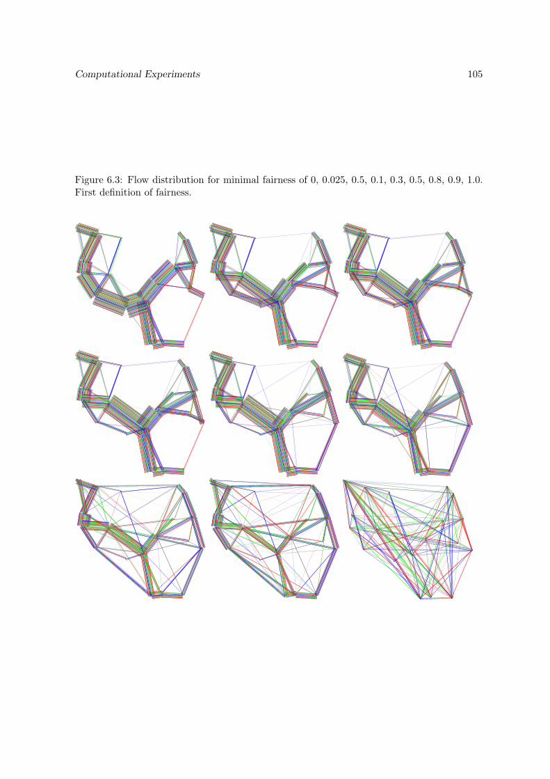
Computational Experiments 105
Figure 6.3: Flow distribution for minimal fairness of 0, 0.025, 0.5, 0.1, 0.3, 0.5, 0.8, 0.9, 1.0.First definition of fairness.

106 On the Fairness of ad-hoc Telecommunication Networks
Figure 6.4: Total energy consumption and fairness. Comparison between first and seconddefinition of fairness.
0
5000
10000
15000
20000
25000
0 0.1 0.2 0.3 0.4 0.5 0.6 0.7 0.8 0.9 1
Fairness
En
erg
y
II def., alpha=2
I def., alpha=2
II def.,_alpha=3
I def., alpha=3
II def., alpha=4
I def., alpha=4
larger fairness is imposed, there are always nodes whose energy cost is decreasing, i.e. thathave a real benefit when larger fairness is imposed.
The graph of Figure 6.7 considers the same network, but now the transmitting distanceequals 4/10 of the 10X10 square, and power control is not used. Thus, all existing linkshave the same cost (= 1 in our experiment). It is very interesting to node that a fairness ofapproximately 0.4 can be obtained ”for free” (i.e., without energy cost increase for the systemas a whole, but simply distributing the flow in a different way). This means that, among themany feasible routing of minimum cost, there is one that is quite fair.
6.3.3 Access Point Configuration
In this Section a different traffic configuration is considered, representing a network wherethe nodes talk only to a server, i.e. all commodities are originated from or directed to aserver. This configuration can describe laptops accessing the Internet via a wireless connectionthrough an Access Point (server). Since α ∈ [2, 8], even if a node can communicate directlyto the server, it can be less expensive to forward the flow through an intermediate node. Weconsider a centralized control approach of this network.
Nodes are generated with a specified distribution on a surface; with a given probability pt,node i transmits to the server, with a probability pr, node i receives from the server (a nodecan both transmit and receive). The quantity of bits transmitted or received has uniform

Computational Experiments 107
Figure 6.5: Flow distribution for minimal fairness of 0.1, 0.3, 0.5, 0.8 and 1.0. Seconddefinition of fairness.
distribution between 0 and a maximum value (actually it is normalized to 1). We considerthe case when power control is used.
We can assume that the server is connected to a power supply system, and than the energyit spends does not represent a cost for the system. For the same reason (and because theserver is always transmitting its own traffic), fairness of the server is disregarded (which isalways equal to 1 when measured according to the first definition (6.7)).
In this kind of network, the second measure of fairness (6.10) is useless, actually, in noefficient solution nodes close to the server can be in a fair condition, unless they simply do notforward other node’s traffic. Imposing such kind of fairness would produce useless solution,where flows having as destination nodes close to the server (which could be directly sent withno cost) would take long routes only to reduce the unbalance of such nodes.
The first definition seems more meaningful, since this configuration is unbalanced bydefinition (unlucky nodes is the middle have to forward). Imposing a minimum fairness wouldaffect the quantity of flow that is routed through long arcs instead of using short connectionwith overloaded neighbors, and would balance the flow among forwarding nodes.
The numerical example considered has 30 nodes: 1 server in the center and 29 users withuniform distribution on a 10X10 square. The server transmits to all nodes (pr = 1), while 60%of the nodes transmit to the server (pt = 0.6). No constraint is imposed on the battery of the

108 On the Fairness of ad-hoc Telecommunication Networks
Figure 6.6: Energy consumption of the single nodes and fairness, power control. Seconddefinition of fairness.
0
100
200
300
400
500
600
700
0 0.1 0.2 0.3 0.4 0.5 0.6 0.7 0.8 0.9 1
Fairness
En
erg
y
nodes, and power control is used. In the graph of Figure 6.8 we consider 3 different values of α,namely α = 2, 3, 4. The maximum transmitting power is set in such a way that the maximumtransmitting distance equals 3/10, 4/10 and 10/10 of the 10X10 square. The total energy costof the solution (log) is reported for different values of fairness. In this configuration, imposingfairness has a large cost in terms of energy spent by the system, however, moderate levels offairness can be obtained with acceptable energy cost. Not surprisingly, for a given value of αand φ, reducing the maximum transmitting power increases the energy cost, because less arcsare available on the network. When a high level of fairness is required, the problem becomesinfeasible (and the corresponding curve is interrupted in the graph of Figure 6.8).
The pictures of Figure 6.9 represent the flow on the network, in the case of α = 4 andmaximum transmitting distance equal to 4/10 of the 10X10 square, when increasing values offairness are imposed. The last picture (α = 1.0), which does not represent a feasible solutionbecause arcs that are not available in the network are used, is reported to visualize the ODpairs. It can be noticed that the flows tend to be routed on few efficient paths when fairnessis disregarded, while it is split on many path when a more fair solution is imposed.

A Distributed Routing Algorithm 109
Figure 6.7: Energy consumption of the single nodes and fairness, no power control. Seconddefinition of fairness.
0
5
10
15
20
25
0 0.1 0.2 0.3 0.4 0.5 0.6 0.7 0.8 0.9 1
Fairness
En
erg
y
6.4 A Distributed Routing Algorithm
The model described in the previous Sections can be used to compute the most efficientsolution for the system, under fairness constraint. It considers a static system, and requiressome kind of centralized control. Moreover, it requires that all the traffic to be transmittedduring a given time interval is known in advance. Conversely, ad hoc network are decentralizednetworks where:
• there is no centralized system control;
• only local information is available at node level;
• decisions are taken ”on line”, without knowledge of the future traffic.
This means that decentralized algorithms, using only local information, must be consideredwhen routing packets through these networks. These algorithms, using only local informationand decentralize control, won’t possibly reach the maximal theoretical efficiency, which shouldbe considered as a benchmark on the system performance.
In absence of node capacity (battery) and fairness constraints, the best routing for eachcommodity is the one using the shortest path. Our proposal is to continue using shortest path

110 On the Fairness of ad-hoc Telecommunication Networks
Figure 6.8: Total energy consumption (log) and fairness. Access point configuration, firstdefinition of fairness.
100
1000
10000
0 0.1 0.2 0.3 0.4 0.5 0.6 0.7 0.8 0.9 1
Fairness
En
erg
y
alpha=2, 3/10
alpha=2, 4/10
alpha=2, 10/10
alpha=3, 3/10
alpha=3, 4/10
alpha=3, 10/10
alpha=4, 3/10
alpha=4, 4/10
alpha=4, 10/10
connections between origins and destinations, by changing the cost of each arc according tothe unbalance and remaining batteries of its endpoints. Shortest path routing protocols arequite common in telecommunications (see, e.g., the routing protocol for ad hoc networksdefined by Johnson, Maltz and Broch [69]), and we can use any of them in a transparent way,the only difference being the cost for the use of each arc.
In a dynamic setting, the flow changes over time and thus the routing should be updated atperiodic intervals. When a node receives a packet to be routed to a destination, it will decide”on line”, according to the actual costs of the arcs, which path to use. At the update, eachnode computes its current unbalance and remaining battery, and the costs of its connectionsare updated accordingly. Let i, j be an edge of the network, and define the original cost of thisedge as the unitary energy cost: cij = ρ + δij , or cij = ρ + 1 when power control is not used.If remaining batteries and fairness are disregarded, these are the costs to be used to computethe shortest path routing. If we want to take into consideration also remaining capacitiesand fairness, the cost of each arc can be defined as: cij = cij/f(ri, rj , p(i), p0(i), p(j), p0(j)),where ri is the fairness of node i, and p(i) and p0(i) represent the remaining and starting (ormaximum) batteries of node i, respectively.
The function f(ri, rj , p(i), p0(i), p(j), p0(j)) should have the following properties:
• f() ≥ 0, in order to avoid the use of long inefficient paths, only to reduce the solution’scost;

A Distributed Routing Algorithm 111
Figure 6.9: Flow distribution for minimal fairness of 0.0, 0.1, 0.3, 0.5, 0.8 and 1.0. Accesspoint configuration.
• f(ri, rj , p0(i), p0(i), p0(j), p0(j)) = 1, because we imagine the fairness to be an issue onlyfor nodes with scarce battery;
• increasing w.r.t. ri (a large value of ri means that i is not contributing to the network);
• increasing w.r.t. p();
Using this kind of routing protocol requires each node to be able to know its unbalance,in order to compute its fairness and the transmitting cost of its connections. While each nodeknows its remaining battery and how much energy it is spending to forward other node’spackets (the negative components of its unbalance), a mechanism has to be designed in orderto let the node know how much energy other nodes are spending for it. Consider a commodityst: in Section 6.2.2 we defined Sq and Rq as the quota of the energy cost which are imputedto the origin s and the destination t, respectively. When all the energy cost is imputed tothe receiver, forwarding nodes can simply add a ”receipt” to forwarded packets (or update astring storing the total transmission cost of the packet, up to the actual node), in order tolet the receiver know how much they worked for it (the receiver must know only the totalamount of energy spent). When the sender too has to pay for the transmission (i.e. Sq > 0),the receipt can be sent back from the receiver to the sender.

112 On the Fairness of ad-hoc Telecommunication Networks
6.4.1 Experimental Results
The static setting considered in this paper, where all the demand matrix is optimized at onceand the traffic is sent on the less expensive paths, satisfying a required fairness level andoptimizing the global cost, is the best solution for the system. It needs a central control,and in addition it requires that all the traffic to be transmitted is known in advance, whichis possibly a stronger assumption. Conversely, the distributed routing algorithm that wesketched in the previous Section requires only local information, and the routing decisioncan be taken ”on line”, by considering the actual cost of the arcs (depending on the historyof the system). A way to compare the performance of the decentralized algorithm with thebenchmark, is to consider an OD matrix and transmit it by using the decentralized routingalgorithm. However, the question is how one can imagine the transmission to be scheduled: inthe static centralized setting, everything is optimized simultaneously, while the decentralizedrouting algorithm works ”on line”, the actual routing depending on the actual arcs costs, i.e.on the previous history.
Concerning the scheduling of the transmission, we can imagine to route a given fractionof all the OD matrix (the same fraction for all commodities), then update the arcs’ costs,and route the next fraction, until the whole OD matrix has been routed. The advantageof this procedure is that the final routing does not depend on the order the commoditiesare considered, but only depends on the fraction that is routed between two consecutiveupdates (or, in other words, depends on the frequency of update). This procedure gives theperformance of the decentralized algorithm when the traffic between each OD pair does notchange over time, which is the static situation solved by the centralized approach, thus beinga fair comparison. We can imagine that the OD matrix represents the traffic of a long timeinterval, and many updates of the arcs’ cost are be performed during the transmission of thematrix.
Some numerical examples are discussed in the following. To keep the analysis simple,we do not consider the remaining batteries of the nodes. The OD matrix has to be sent inone time period, and let freq be the frequency we update the arcs’ costs in the time period;update = 1/freq is the number of updates performed in the period. The decentralizedalgorithm is applied in the following way:
begin1. iter=1;2. while (iter ≤ update)3. for all commodities st ∈ K4. p := shortest path(s, t);4. send dst/update on p;5. endfor;6. update arcs’ costs;7. endwhile;
In order to compute the arcs’ costs cij = cij/f(ri, rj , p(i), p0(i), p(j), p0(j)), we definef(ri, rj , ., ., ., .) = (δij ri + ρ rj)β (δij = 1 when power control is not used), where β isa parameter to be experimentally tuned, which represents the importance that is given tofairness in the solution.

A Distributed Routing Algorithm 113
In the following examples, we consider the same network of Section 6.3.2 and we run thedecentralized algorithms with increasing values of β. We report curves describing the costof the solutions as function of the corresponding fairness. It’s worth noting that, while inmodel (6.11)- (6.17) the fairness is imposed as a constraint, and thus it is know a priori, whenusing the decentralized algorithm we can set only the value of β, obtaining the cost and thefairness of the corresponding solution as an output. In other words, there is no guarantee onthe minimum fairness of the network, but only a parameter to increase the importance givento fairness in the routing. In our experiments, we start by setting β = 0 (i.e. we route everycommodity on the shortest path) and we iteratively increase it by 0.1 steps until β ∈ [0, 1] ,and of 1.0 steps when β > 1.
In the first example, we consider the usual network of 20 nodes, generated with uniformprobability on a 10X10 square, each one participating in the network (i.e. transmitting orreceiving some traffic). The probabilities pt and pr are set to 0.6 and 0.7, respectively. Thequantity of bits transmitted between each OD pair has uniform distribution between 0 and amaximum value (actually it is normalized to 1). The battery of nodes is not a constraint (i.e.every node has enough capacity), power control is used. We perform 50 updates of the arcs’cost during the transmission.
The graph of Figure 6.10 reports in purple the curve representing the total energy costof solutions found by the decentralized algorithm, with respect to the minimal fairness ex-perienced by a node of the network (the second definition of fairness 6.10 being used), forincreasing values of the parameter β. The curve can be compared with the benchmark curve(blue), representing the solutions of model (6.11)- (6.17) when different levels of fairness areimposed (note that in this case back arcs are allowed, because they can be used by the de-centralized algorithm). Even if the decentralized algorithm curve is in general monotone (byincreasing β the corresponding fairness and cost are increased), this is not always true, espe-cially for large values of β. The performance of the decentralized algorithm is close, at leastfor values of fairness up to 0.7, to the benchmark, showing the effectiveness of the proposedrouting algorithm.
The graph of Figure 6.11 reports the distribution of energy costs among the 20 nodesof the network, with respect to the minimal fairness experienced by a node of the network.The red dashed curve reports the average cost. For quite high levels of fairness, there arestill nodes whose energy is decreasing. This means that the solution is really useful, i.e. thefairness is not only obtained by making some nodes perform useless extra work, but it is reallyobtained by reducing the cost for nodes working too much. When β is very large, we can getsolutions close to 0.9% fair. However, in this case all nodes are spending more energy thatthey would in less fair solutions, which are actually more desirable.
We then consider the same network, without using power control, i.e. all existing arcshave cost 1. The maximum transmitting power pMax is set large enough to let every nodereach all nodes within a distance equal to 4/10 of the diagonal of the square.
In the graph of Figure 6.12 the performance of the decentralized algorithm (purple curve)is compared with the benchmark. It is very interesting to node that a fairness of approximately40% can be obtained ”for free” in this example. This means that, among the many feasiblerouting of minimum cost, there is one that is quite fair, and the decentralized algorithm isable to find it. When we search for larger fairness, this has a cost, but the performance ofthe algorithm is still comparable with the benchmark.
The graph of figure 6.13 reports the distribution of energy costs among the 20 nodes ofthe network. The red dashed curve reports the average cost. The first ”gap” in the graph,

114 On the Fairness of ad-hoc Telecommunication Networks
Figure 6.10: Total energy consumption and fairness, power control. Decentralized Algorithmand Benchmark.
60
80
100
120
140
160
180
0.08 0.18 0.28 0.38 0.48 0.58 0.68 0.78 0.88 0.98
Fairness
En
erg
y
benchmark
decentralized alg.
corresponding to an increase of the value β from 0 to 0.1, shows that this is enough to leadthe algorithm to a fair solution, among the many equivalent solution of minimum cost.
6.5 Conclusions
Wireless ad hoc networks, where nodes communicate without making use of any preexistinginfrastructure and centralized control, will be highly pervasive in the next future. A wideliterature is available on ad-hoc networks, mainly devoted to the study of the efficiency ofnetworks, and to the design of mechanisms to obtain a desired behavior from the networknodes. The efficiency of ad hoc network is highly related to the routing protocols that thenetwork uses. However, the study of the fairness of routing protocols in ad hoc network havebeen rarely considered in the literature, and, to the best of our knowledge, never in a deepway.
In this paper we propose a possible model for the routing of information packets in wirelessad hoc networks, where the objective is the design of the most efficient routing, i.e. the one

Conclusions 115
Figure 6.11: Energy consumption of the single nodes and fairness, power control. Decentral-ized Algorithm.
0
50
100
150
200
250
300
0.1 0.2 0.3 0.4 0.5 0.6 0.7 0.8 0.9
Fairness
En
erg
y
of minimum energy cost. We define two alternative measures for the fairness of a routing insuch networks, and discuss how an efficient routing can be computed by satisfying a minimumfairness constraint, basically through the solution of a Linear Programming Model. Thecomputation of this routing, however, requires a set of information which is normally notavailable at single node level, where the routing decisions are taken. Thus, it can be consideredas a benchmark on the best possible routing, and could be implemented only by a centralizedcontrol of the system, which is impossible for the intrinsic decentralized nature of ad hocnetwork.
So, we propose also a distributed routing algorithm, which uses only local information,available at node level. The algorithm is aimed at computing an efficient routing, while takinginto consideration the fairness experienced by the nodes in the network.
Extensive computational experiments on randomly generated networks show that themeasure of fairness we propose are meaningful, leading a true reduction on the energy con-sumption of some nodes of the network, with an acceptable loss in the network efficiency. Inaddition, the distributed fair routing algorithm that we propose is able to find fair routings,by using only locally available information, with a performance which is comparable to thebenchmark, i.e. to the routing which could be computed by a centralized control algorithm,by solving a Linear Program.

116 On the Fairness of ad-hoc Telecommunication Networks
Figure 6.12: Total energy consumption and fairness, no power control. Decentralized Algo-rithm and Benchmark.
8
9
10
11
12
13
14
15
16
0.15 0.25 0.35 0.45 0.55 0.65 0.75 0.85 0.95
Fairness
En
erg
y
benchmark
decentralized alg.

Conclusions 117
Figure 6.13: Energy consumption of the single nodes and fairness, no power control. Decen-tralized Algorithm.
0
5
10
15
20
25
0.16 0.26 0.36 0.46 0.56 0.66 0.76
Fairness
En
erg
y

118 On the Fairness of ad-hoc Telecommunication Networks

Bibliography
[1] ftp://dimacs.rutgers.edu/pub/challenge/graph/.
[2] http://fap.zib.de/index.php.
[3] http://www-di.inf.puc-rio.br/ celso/grupo de pesquisa.htm.
[4] K.I. Aardal, C.P.M. van Hoesel, A.M.C.A. Koster, C. Mannino, and A. Sassano. Modelsand solution techniques for the frequency assignment problem. ZIB-report 01–40, Berlin,Germany, 2001.
[5] Y. Afek, Y. Mansour, and Z. Ostfeld. Convergence complexity of optimistic rate basedflow control algorithms (extended abstract). In STOC ’96: Proceedings of the twenty-eighth annual ACM symposium on Theory of computing, pages 89–98, New York, NY,USA, 1996. ACM Press.
[6] Y. Afek, Y. Mansour, and Z. Ostfeld. Phantom: a simple and effective flow controlscheme. In SIGCOMM ’96: Conference proceedings on Applications, technologies, ar-chitectures, and protocols for computer communications, pages 169–182, New York, NY,USA, 1996. ACM Press.
[7] D. Alvin. Punishment in selfish wireless networks: a game theoretic analysis. In Pro-ceedings of the Workshop on the Economics of Networked Systems (NetEcon 2006),2006.
[8] L. Anderegg and S. Eidenbenz. Ad hoc-vcg: a truthful and cost-efficient routing protocolfor mobile ad hoc networks with selfish agents. In MobiCom ’03: Proceedings of the 9thAnnual International Conference on Mobile Computing and Networking, pages 245–259,New York, NY, USA, 2003. ACM Press.
[9] L.G. Anderson. A simulation study of some dynamic channel assignment algorithms ina high capacity mobile telecommunications system. IEEE Transactions on Communi-cations, 21:1294–1301, 1973.
[10] K. Appel, W. Haken, and J. Koch. Every planar map is four colorable. Illinois Journalof Mathematics, 21:439–567, 1977.
[11] B.S. Baker and E.G. Coffman. Mutual exclusion scheduling. Theoretical ComputerScience, 162:225–243, 1996.
[12] V.C. Barbosa, C.A.G. Assis, and J.O. Do Nascimento. A range-compaction heuristicfor graph coloring. Journal of Combinatorial Optimization, 8:41–63, 2004.
119

120 BIBLIOGRAPHY
[13] D. Bertsekas and R. Gallager. Data Networks. Prentice Hall, 1992.
[14] R. Bhargava, A. Goel, and A. Meyerson. Using approximate majorization to characterizeprotocol fairness. In SIGMETRICS/Performance, pages 330–331, 2001.
[15] I. Blochliger and N. Zufferey. A reactive tabu search using partial solutions for the graphcoloring problem. Technical Report 04/03, Ecole Polytechnique Federale de Lausanne(EPFL), Recherche Operationnelle Sud-Est (ROSE), CH-1015 Lausanne, Switzerland,2004.
[16] L. Bodin, B. Golden, A. Assad, and M. Ball. Routing and scheduling of vehicles andcrews: the state of the art. Computers & Operations Research, 10:63–211, 1983.
[17] H.L. Bodlaender and K. Jansen. On the complexity of scheduling incompatible jobswith unit-times. In MFCS ’93: Proceedings of the 18th International Symposium onMathematical Foundations of Computer Science, pages 291–300, London, UK, 1993.Springer-Verlag.
[18] B. Bollobas and A. Thomason. Random graphs of small order. Annals of DiscreteMathematics, 28:47–97, 1985.
[19] M. Boudhar and G. Finke. Scheduling on a batch machine with job compatibilities.Belgian Journal of Operations Research, Statistics and Computer Science, 40(1-2):874–885, 2000.
[20] D. Brelaz. New methods to color the vertices of a graph. Communications of the ACM,22(4):251–256, 1979.
[21] S. Buchegger and J. Le Boudec. Nodes bearing grudges: Towards routing security,fairness, and robustness in mobile ad hoc networks. In Proceedings of the 10th EuromicroWorkshop on Parallel, Distributed and Network-based Processing (PDP2002).
[22] S. Buchegger and J. Le Boudec. Performance analysis of the confidant protocol. InMobiHoc ’02: Proceedings of the 3rd ACM international symposium on Mobile ad hocnetworking & computing, pages 226–236, New York, NY, USA, 2002. ACM Press.
[23] A. Caprara, M. Fischetti, and P. Toth. A heuristic method for the set covering problem.Operations Research, 47:730–743, 1999.
[24] A. Caprara and P. Toth. Lower bounds and algorithms for the 2-dimensional vectorpacking problem. Discrete Applied Mathematics, 11:231–262.
[25] M. Caramia and P. Dell’Olmo. A fast and simple local search for graph coloring. Proc.of the 3d Workshop on Algorithm Engineering WAE’99, Lecture Notes in ComputerScience, 1668:319–313, 1999.
[26] M. Caramia and P. Dell’Olmo. Constraint propagation in graph coloring. Journal ofHeuristics, 8:83–107, 2002.
[27] M. Caramia and P. Dell’Olmo. Bounding vertex coloring by truncated multistage branchand bound. Networks, 44(4):231–242, 2004.

BIBLIOGRAPHY 121
[28] G. Carpaneto, S. Martello, and P. Toth. Algorithms and codes for the assignmentproblem. Annals of Operations Research, 13:193–223, 1988.
[29] M.W. Carter, G. Laporte, and S.Y. Lee. Examination timetabling: Algorithmic strate-gies and applications. Journal of the Operational Research Society, 47:373–383, 1996.
[30] F.C. Chow and J.L. Hennessy. The priority-based coloring approach to register allo-cation. ACM Transactions on Programming Languages and Systems, 12(4):501–536,1990.
[31] N. Christofides, A. Mingozzi, and P. Toth. The vehicle routing problem. InN. Christofides, A. Mingozzi, P. Toth, and C. Sandi, editors, Combinatorial Optimiza-tion, pages 315–338. Wiley, Chichester, 1979.
[32] B.G. Chun, R. Fonseca, I. Stoica, and J. Kubiatowicz. Characterizing selfishly con-structed overlay routing networks. In Proceedings of 23rd IEEE International Confer-ence on Computer Communications (INFOCOM 2004), volume 2, pages 1329–1339,2004.
[33] E.G. Coffman, M.R. Garey, and D.S. Johnson. Approximation algorithms for bin-packing - an updated survey. In G. Ausiello, M. Lucentini, and P. Serafini, editors,Algorithm Design for Computer System Design, pages 49–106. Springer, Vienna, 1984.
[34] J.R Correa, A.S. Schulz, and N. Stier Moses. Selfish routing in capacitated networks.Mathematics of Operations Research, 29(4):961–976, 2004.
[35] J.R Correa, A.S. Schulz, and N. Stier Moses. Fast, fair and efficient flows in networks.Operations Research (to appear), 2007.
[36] D. Costa. On the use of some known methods for T-colourings of graphs. Annals ofOperations Research, 41:343–358, 1993.
[37] J.C. Culberson and F. Luo. Exploring the k-colorable landscape with iterated greedy.In D.S. Johnson and M.A. Trick, editors, Cliques, Coloring, and Satisfiability: 2ndDIMACS Implementation Challange, 1993, DIMACS Series in Discrete Mathematicsand Theoretical Computer Science. American Mathematical Society, 1996.
[38] L. Davis. Handbook of Genetic Algorithms. Van Nostrand Reinhold, New York, 1998.
[39] D. de Werra. An introduction to timetabling. European Journal of Operational Research,19:151–162, 1985.
[40] D. De Werra, M. Demange, J. Monnot, and V.T. Paschos. Time slot scheduling ofcompatible jobs. Journal of Scheduling, 2006. (to appear).
[41] I.M. Diaz and P. Zabala. A branch and cut algorithm for graph coloring. In Computa-tional Symposium on Graph Coloring and its Generalization, pages 55–62, Ithaca, NewYork, 2002.
[42] J.J. Dongarra. Performance of various computers using standard linear equations soft-ware, (linpack benchmark report). Technical Report CS-89-85, University of Tennessee,Computer Science Department, 2005.

122 BIBLIOGRAPHY
[43] R. Dorne and J.K. Hao. Tabu search for graph coloring, t-coloring and set t-colorings. InS. Voss, S. Martello, I.H. Osman, and C. Roucairol, editors, Meta-Heuristics: Advancesand Trends in Local Search Paradigms for Optimization. Kluwer Academic Publishers,Boston, 1998.
[44] S. Eidenbenz, V.S.A. Kumar, and S. Zust. Equilibria in topology control games for adhoc networks. Mobile Networks Applications, 11(2):143–159, 2006.
[45] B. Escoffier, J. Monnot, and V.T. Paschos. Weighted coloring: further complexity andapproximability results. Information Processing Letters, 94(3):98–103, 2006.
[46] E. Falkenauer. A hybrid grouping genetic algorithm. Journal of Heuristics, 2:5–30,1996.
[47] A.E. Fernandez Muritiba, M. Iori, E. Malaguti, and P. Toth. Lower and upper boundsfor the bin packing problem with conflicts. Technical Report OR/06/7, DEIS Universityof Bologna, 2005.
[48] G. Finke, V. Jost, M. Queyranne, and A. Sebo. Batch processing with interval graphcompatibilities between tasks. Cahiers du laboratoire Leibniz, 108, 2004.
[49] C. Fleurent and J.A. Ferland. Object-oriented implementation of heuristic search meth-ods for graph coloring. In D.S. Johnson and M.A. Trick, editors, Cliques, Coloring, andSatisfiability: 2nd DIMACS Implementation Challange, 1993, DIMACS Series in Dis-crete Mathematics and Theoretical Computer Science. American Mathematical Society,1996.
[50] N. Funabiki and T. Higashino. A minimal-state processing search algorithm for graphcoloring problems. IEICE Trans. Fundamentals, E83-A(7):1420–1430, 1990.
[51] P. Galinier and J.K. Hao. Hybrid evolutionary algorithms for graph coloring. Journalof Combinatorial Optimization, 3(4):379–397, 1999.
[52] A. Gamst. Some lower bounds for a class of frequency assignment problems. IEEETransactions on Vehicular Technology, 35(1):8–14, 1986.
[53] M.R. Garey and D.S. Johnson. Computers and Intractability: A Guide to the Theory ofNP-Completeness. DIMACS Series in Discrete Mathematics and Theoretical ComputerScience. Freedman, New York, 1979.
[54] H. Gavranovich and G. Finke. Graph partitioning and set covering for the optimaldesign of a production system in the metal industry. In Proceedings of the SecondConference on Management and Control of Production and Logistics (MCPL’2000),volume 2, pages 603–608, Grenoble, France, 2000.
[55] M. Gendreau, G. Laporte, and F. Semet. Heuristics and lower bounds for the binpacking problem with conflicts. Computers & Operations Research, 31:347–358, 2004.
[56] P.C. Gilmore and R.E. Gomory. A linear programming approach to the cutting stockproblem. Operations Research, 9:849–859, 1961.
BIBLIOGRAPHY 123
[57] P.C. Gilmore and R.E. Gomory. A linear programming approach to the cutting stockproblem – Part II. Operations Research, 11:863–888, 1963.
[58] A. Goel, A. Meyerson, and S. Plotkin. Combining fairness with throughput: onlinerouting with multiple objectives. In STOC ’00: Proceedings of the thirty-second annualACM symposium on Theory of computing, pages 670–679, New York, NY, USA, 2000.ACM Press.
[59] A. Goel, A. Meyerson, and S. Plotkin. Approximate majorization and fair online loadbalancing. ACM Transactions on Algorithms, 1(2):338–349, 2005.
[60] P. Hansen, A. Hertz, and J. Kuplinsky. A range-compaction heuristic for graph coloring.Journal of Combinatorial Optimization, 8:41–63, 2004.
[61] J.K. Hao, R. Dorne, and P. Galinier. Tabu search for frequency assignment in mobileradio networks. Journal of Heuristics, 4:47–62, 1998.
[62] A. Hertz and D. de Werra. Using tabu search techniques for graph coloring. Computing,39:345–351, 1987.
[63] D.S. Hochbaum and D. Landy. Scheduling semiconductor burn-in operations to mini-mize total flowtime. Operations Research, 45(6):874–885, 1997.
[64] J. Jaffe. Bottleneck flow control. IEEE Transactions on Communications, 29(7):954–962, 1981.
[65] O. Jahn, R.H. Mohring, Schulz A.S., and N. Stier Moses. System-optimal routing oftraffic flow with user constraints in networks with congestion. Operations Research,53(4):600–616, 2005.
[66] K. Jansen. An approximation scheme for bin packing with conflicts. Journal of Com-binatorial Optimization, 3:363–377, 1999.
[67] K. Jansen and S. Oehring. Approximation algorithms for time constrained scheduling.Information and Computation, 132:85–108, 1997.
[68] H. Ji and C.Y. Huang. Non-cooperative uplink power control in cellular radio systems.Wireless Networks, 4(3):233–240, 1998.
[69] D.B. Johnson, D.A. Maltz, and J. Broch. DSR: The dynamic source routing protocolfor multi-hop wireless ad hoc networks. In C. E. Perkins, editor, Ad Hoc Networking.Addison-Wesley, 2001.
[70] D.S. Johnson. Near-optimal bin packing algorithms. PhD thesis, MIT, Cambridge, MA,1973.
[71] D.S. Johnson. Approximation algorithms for combinatorial problems. Journal of Com-puters and System Science, 9:256–278, 1974.
[72] D.S. Johnson, C.R. Aragon, L.A. McGeoch, and C. Schevon. Optimization by simulatedannealing: an experimental evaluation; Part II, graph coloring and number partitioning.Operations Research, 39(3):378–406, 1991.

124 BIBLIOGRAPHY
[73] D.S. Johnson and M.A. Trick (eds.). Cliques, Coloring, and Satisfiability: 2nd DI-MACS Implementation Challange, 1993. DIMACS Series in Discrete Mathematics andTheoretical Computer Science. American Mathematical Society, 1996.
[74] D.E. Joslin and D.P. Clements. Squeaky wheel optimization. Journal of ArtificialIntelligence Research, 10:353–373, 1999.
[75] J.P. Kelly and J. Xu. A set-partitioning-based heuristic for the vehicle routing problem.INFORMS Journal on Computing, 11(2):161–172, 1999.
[76] A. Kesselman, D. Kowalski, and M. Segal. Energy efficient communication in ad hocnetworks from user’s and designer’s perspective. SIGMOBILE Mob. Comput. Commun.Rev., 9(1):15–26, 2005.
[77] J.M. Kleinberg, E. Tardos, and Y. Rabani. Fairness in routing and load balancing. InFOCS ’99: Proceedings of the 40th Annual Symposium on Foundations of ComputerScience, pages 568–578, Washington, DC, USA, 1999. IEEE Computer Society.
[78] G. Laporte and S. Desroches. Examination timetabling by computer. Computers &Operations Research, 11:351–360, 1984.
[79] J.W. Lee, R.R. Mazumdar, and N.B. Shroff. Downlink power allocation for multi-classwireless system. IEEE/ACM Transactions on Networking, 13(4):854–867, 2005.
[80] F.T. Leighton. A graph coloring algorithm for large sceduling problems. Journal ofResearch of the National Bureau of Standards, 84(6):489–503, 1979.
[81] A. Lim, Q. Lou, B. Rodrigues, and Y. Zhu. Heuristic methods for graph coloringproblems. In Proceedings of the 2005 ACM Symposium on Applied Computing, pages933–939, Santa Fe, Nex Mexico, 2005.
[82] A. Lim, X. Zhang, and Y. Zhu. A hybrid methods for the graph coloring and itsrelated problems. In Proceedings of MIC2003: The Fifth Metaheuristic InternationalConference, Kyoto, Japan, 2003.
[83] A. Lodi, S. Martello, and D. Vigo. Models and bounds for two-dimensional level packingproblems. Journal of Combinatorial Optimization, 8:363–379, 2004.
[84] E. Malaguti, M. Monaci, and P. Toth. A metaheuristic approach for the vertex coloringproblem. Technical Report OR/05/3, DEIS University of Bologna, 2005.
[85] E. Malaguti, M. Monaci, and P. Toth. A set-covering based approach for a weightedvertex coloring problem. Technical Report OR/06/04, DEIS University of Bologna,2005.
[86] E. Malaguti and P. Toth. An evolutionary approach for bandwidth multicoloring prob-lems. European Journal of Operational Research (to appear), 2007.
[87] R. Marsten and F. Shepardson. Exact solution of crew scheduling problems using theset partitioning model: recent successful applications. Networks, 112:167–177, 1981.
[88] S. Martello and P. Toth. Knapsack Problems: Algorithms and Computer Implementa-tions. John Wiley & Sons, Chichester, 1990.

BIBLIOGRAPHY 125
[89] S. Marti, T.J. Giuli, K. Lai, and M. Baker. Mitigating routing misbehavior in mobile adhoc networks. In Proceedings of the Sixth annual ACM/IEEE International Conferenceon Mobile Computing and Networking, pages 255–265, 2000.
[90] A. Mehrotra and M.A. Trick. A column generation approach for graph coloring. IN-FORMS Journal on Computing, 8:344–354, 1996.
[91] M. Monaci and P. Toth. A set-covering based heuristic approach for bin-packing prob-lems. INFORMS Journal on Computing, 18:71–85, 2006.
[92] C.A. Morgenstern. Distibuted coloration neighborhood search. In D.S. Johnson andM.A. Trick, editors, Cliques, Coloring, and Satisfiability: 2nd DIMACS ImplementationChallange, 1993, DIMACS Series in Discrete Mathematics and Theoretical ComputerScience. American Mathematical Society, 1996.
[93] V. Phan and S. Skiena. Coloring graphs with a general heuristic search engine. In Com-putational Symposium on Graph Coloring and its Generalization, pages 92–99, Ithaca,New York, 2002.
[94] M. Prais and C.C. Ribeiro. Reactive GRASP: An application to a matrix decompositionproblem in TDMA traffic assignment. INFORMS Journal on Computing, 12(3):164–176, 2000.
[95] S. Prestwich. Constrained bandwidth multicoloration neighborhoods. In ComputationalSymposium on Graph Coloring and its Generalization, pages 126–133, Ithaca, New York,2002.
[96] S. Prestwich. Generalized graph colouring by a hybrid of local search and constraintprogramming. Technical report, Cork Constraint Computation Center, Ireland, 2005.
[97] D. Wetherall R. Mahajan, M. Rodrig and J. Zahorjan. Sustaining cooperation in multi-hop wireless networks. In Proocedings of the Second USENIX Symposium on NetworkedSystem Design and Implementation (NSDI 05), 2005.
[98] T.S. Rappaport. Wireless Communications: Principles and Practices. Prentice Hall,1996.
[99] C.C. Ribeiro, M. Minoux, and M.C. Penna. An optimal column-generation-with-rankingalgorithm for very large scale set partitioning problems in traffic assignment. EuropeanJournal of Operational Research, 41:232–239, 1989.
[100] F.S. Roberts. T -colorings of graphs: Recent results and open problems. Discrete Math-ematics, 93:229–245, 1991.
[101] T.J. Sager and S. Lin. A pruning procedure for exact graph coloring. ORSA Journalon Computing, 3(3):226–230, 1991.
[102] A.S. Schulz and N. Stier Moses. Efficiency and fairness of system-optimal routing withuser constraints. Networks, 48(4):223–234, 2006.

126 BIBLIOGRAPHY
[103] E.C. Sewell. An improved algorithm for exact graph coloring. In D.S. Johnson andM.A. Trick, editors, Cliques, Coloring, and Satisfiability: 2nd DIMACS ImplementationChallange, 1993, DIMACS Series in Discrete Mathematics and Theoretical ComputerScience. American Mathematical Society, 1996.
[104] F.C.R. Spieksma. A branch-and-bound algorithm for the two-dimensional vector pack-ing problem. Computers & Operations Research, 21(1):19–25, 1994.
[105] O.K. Tonguz and G. Ferrari. Ad Hoc Wireless Networks: A Communication-TheoreticPerspective. John Wiley & Sons, Chichester, 2006.
[106] M.A. Trick. Computational symposium: Graph coloring and its generalizations, 2002.http://mat.gsia.cmu.edu/COLOR02/.
[107] E. Tsang and C. Voudouris. Solving the radio link frequency assignment problem usingguided local search. In NATO Symposium on Radio Length Frequency Assignment,Aalborg, Denmark, 1998. http://cswww.essex.ac.uk/CSP/papers.html.
[108] C. Velanzuela, S. Hurley, and D. Smith. A permutation based genetic algorithm for theminimum span frequency assignment. Lecture Notes in Computer Science, 1498:907–916, 1999.
[109] J.P. Walser. Feasible cellular frequency assignment using constraint programming ab-stractions. In Proceedings of the Workshop on Constraint Programming Applications(CP96), Cambridge, Massachusetts, USA, 1996.
[110] W. Wang and C.K. Rushforth. An adaptive local-search algorithm for the channel-assignment problem (CAP). IEEE Transactions on Vehicular Technology, 45:459–466,1996.
[111] D. Wedelin. An algorithm for large scale 0-1 integer programming with application toairline crew scheduling. Annals of Operations Research, 57:283–301, 1995.
[112] T.K. Woo, S.Y.W. Su, and R. Newman Wolfe. Resource allocation in a dynamicallypartitionable bus network using a graph coloring algorithm. IEEE Trans. Commun.,39(12):1794–1801, 2002.
[113] S. Zhong, Y. Yang, and J. Chen. Sprite: A simple, cheat-proof, credit-based system formobile ad hoc networks. Technical Report Yale/DCS/TR1235, Department of Com-puter Science, Yale University, 2002.
[114] J.A. Zoellner and C.L. Beall. A breakthrough in spectrum conserving frequency as-signment technology. IEEE Transactions on Electromagnetic Compatiblity, 19:313–319,1977.


![Galli [método completo]](https://static.fdocuments.in/doc/165x107/554e9fe5b4c9055f7b8b4662/galli-metodo-completo.jpg)