XFLR5 Handout
6
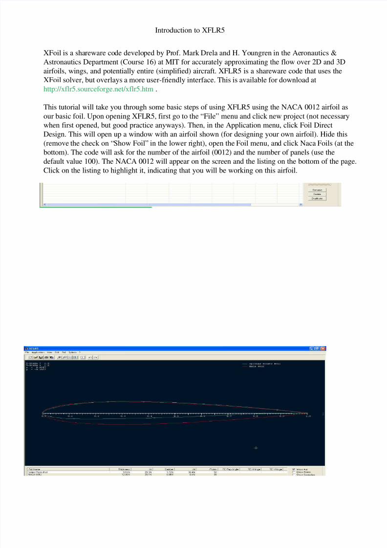
XFoil is a sha reware co de develo ped by Pr of. Mark Drela and H. Yo ungren in the Ae ronautics & Astronautics Department (Course 16) at MIT for accurately approximating the flow over 2D and 3D airfoils, wings, and potentially entire (simplified) aircraft. XFLR5 is a shareware code that uses the XFoil solver, but overlays a more user-fr iendly interface. This is available for download at http://xflr5.sourceforge.net/xflr5.htm . This tutorial will take you through some basic steps of using XFLR5 using the NACA 0012 airfoil as our basic foil. Upon opening XFL R5, first go to the “File” menu and click new project (not necessa ry when first opened, but good practice anyways). Then, in the Application menu, click Foil Direct Design. This will open up a window with an airfoil shown (for designing your own airfoil). Hide this (remove the check on “ Show Foil” in the lower right), open the Foil menu, an d click Naca Foils (at the bottom). The code will ask for the number of the airfoil (0012) and the number of panels (use the default value 100). The NACA 0012 will appear on the screen and the listing on the bottom of the page. Click on the listing to highlight it, indicating that you will be working on this airfoil. Introduction to XFLR5
-
Upload
amirkarimi -
Category
Documents
-
view
247 -
download
0
Transcript of XFLR5 Handout
8/6/2019 XFLR5 Handout
http://slidepdf.com/reader/full/xflr5-handout 1/6
XFoil is a shareware code developed by Prof. Mark Drela and H. Youngren in the Aeronautics &
Astronautics Department (Course 16) at MIT for accurately approximating the flow over 2D and 3D
airfoils, wings, and potentially entire (simplified) aircraft. XFLR5 is a shareware code that uses the
XFoil solver, but overlays a more user-friendly interface. This is available for download at
http://xflr5.sourceforge.net/xflr5.htm .
This tutorial will take you through some basic steps of using XFLR5 using the NACA 0012 airfoil as
our basic foil. Upon opening XFLR5, first go to the “File” menu and click new project (not necessary
when first opened, but good practice anyways). Then, in the Application menu, click Foil Direct
Design. This will open up a window with an airfoil shown (for designing your own airfoil). Hide this
(remove the check on “Show Foil” in the lower right), open the Foil menu, and click Naca Foils (at the
bottom). The code will ask for the number of the airfoil (0012) and the number of panels (use the
default value 100). The NACA 0012 will appear on the screen and the listing on the bottom of the page.
Click on the listing to highlight it, indicating that you will be working on this airfoil.
Introduction to XFLR5

8/6/2019 XFLR5 Handout
http://slidepdf.com/reader/full/xflr5-handout 2/6
Next, on the Application menu, click Xfoil Direct Analysis. This will open a window which shows
the pressure profile (c p
v. x / c) plot (but no data yet) and the airfoil shape (if not, click the button
with the plot and airfoil on it next the print button below the menu. To get some data, click on the
Polars menu and then Define Batch Polar. This window allows us to enter key data depending on
the “Type” of the analysis. We will use Type 1, which means providing a Reynolds and Mach
number. Use Re = 1,000,000 and M = 0.00 (which essentially means low Mach number). You can
give this analysis a user-defined name or just use the somewhat cryptic default. Don’t worry aboutthe transition model stuff, just leave as default values. The name of this polar will now appear in
the box next to the NACA 0012 box. Having supplied these values, we can now analyze the flow,
either by using the batch analysis under the Polars menu or the side menu on the right under
Analysis. I will do the later, by specifying α (angle of attack) = 0 (no sequence), and hitting
analyze. The result is now a pressure profile as shown for this case. Now, redo this analysis, but set
the angle of attack (in “start”) to 4.00 (4 degrees). You will now see a second pressure profile
which has two lines, one for the top surface and the other for the bottom. The c p
axis is inverted,
with negative numbers at the top, because in this way the top line will typically correspond to the
upper (suction) surface of the airfoil (where we want lower pressure). Actually, there is an upper
and lower surface line for the zero degree case as well, but since the airfoil is symmetric there is no
difference between the top and bottom profiles, so they overlap. Note also that the airfoil sketch is
now tilted to show the angle of attack.

8/6/2019 XFLR5 Handout
http://slidepdf.com/reader/full/xflr5-handout 3/6
To see other plots, go to Polars, then View, then choose. However, we need more points to make
this interesting, so first go back to the right-hand Analysis section and do a sequence starting at α =
-4 and continuing to α = 20 with a step (∆) of 1 degree. This will yield many more pressure
profiles (the screen is now getting quite crowded; note also that 19 and 20 degrees will not
converge and therefore will not show up), but we will now have well-defined lift and drag curves.
To see them, go to Polars, View, and then choose Cl vs. alpha. This will show the change in lift
with angle of attack. Next, choose Cl v. Cd – this is the lift-drag polar. Finally, click on “user
graph” – this will yield Cl/Cd v. alpha, with a peak at 8 degrees. If you right click on a plot, you
get another menu which allows you to control the plot display. Here, go to Graph and in the
submenu go to Variables. This presents a list of variables with all the plot choices available. There
are also ways to use these menu to zoom, change the axes, and numerous other options. You can
also export data to a text file by using Polar > Current Polar > Export. Note that you can toggle
from the plot screen to the Cp/airfoil screen by using the two buttons next to the “NACA 0012”. I
can also refine the data in critical areas – so I will do another analyze angle sequence from 7 to 16
degrees with a 0.25 step. This rounds off some ot the corners in the previous plots. To further
define the stall angle, I will do a sequence from 13 to 15 degrees, step 0.1. I will also do the same
from 6 to 10 degrees to refine the L/D peak. Using Polars > Current Polar > Export, I get the data
saved to a file, which I can use to get more precise values, such as a stall angle of 13.9 degrees.
8/6/2019 XFLR5 Handout
http://slidepdf.com/reader/full/xflr5-handout 4/6
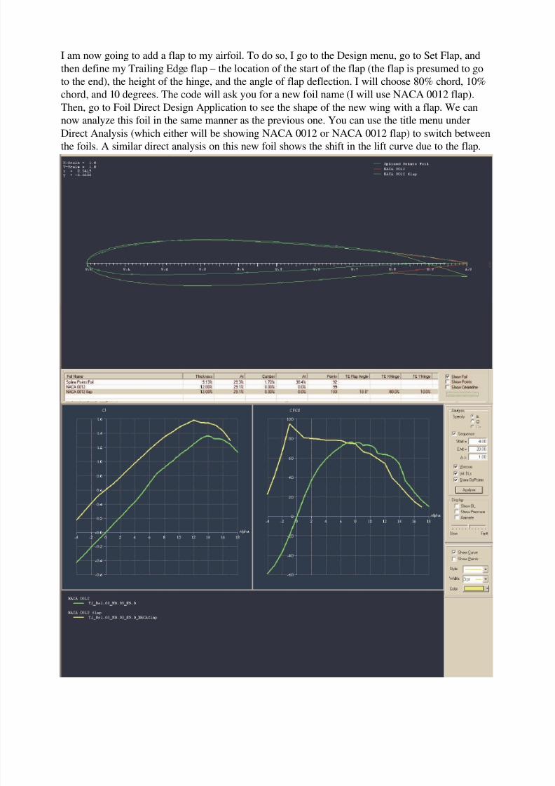
I am now going to add a flap to my airfoil. To do so, I go to the Design menu, go to Set Flap, and
then define my Trailing Edge flap – the location of the start of the flap (the flap is presumed to go
to the end), the height of the hinge, and the angle of flap deflection. I will choose 80% chord, 10%
chord, and 10 degrees. The code will ask you for a new foil name (I will use NACA 0012 flap).
Then, go to Foil Direct Design Application to see the shape of the new wing with a flap. We can
now analyze this foil in the same manner as the previous one. You can use the title menu under
Direct Analysis (which either will be showing NACA 0012 or NACA 0012 flap) to switch betweenthe foils. A similar direct analysis on this new foil shows the shift in the lift curve due to the flap.

8/6/2019 XFLR5 Handout
http://slidepdf.com/reader/full/xflr5-handout 5/6
For the final exercise, I am going to create a wing. For this, I first need to collect enough 2D data
to allow the 3D analysis to work. The best way to do this is to use Polars > Batch Analysis. I will
define a range about my desired freestream Re and a range of angles – this is because in a 3D wing
the Re and angle can change due to sweep, taper, twist, dihedral, and other wing variations. I will
do an analysis on the NACA 0012 (no flap) from Re = 800,000 to 1,200,000, increment 20,000,
and angles -4 to 20 degrees, with an increment of 1 degree. This will take a little while, but not too
long (around 4 minutes on my computer). Occasionally, the results will not converge, but most of
them will. If you keep the Cl plots up, you will quickly see new lines being added for each Re –
these will mostly overlap in the linear region, but will have difference characteristics near stall.
The L/D peak will also shift with Re, due primarily to changes in drag. With this data, the wing
can be analyzed. Go to Application > Wing Design. Under Wing/Plane, go to Define Wing. The
wing is defined by sections starting at the root. The simplest wing has only two Positions, the root
and wingtip. The chord length at each position defines the taper in the wing, the offset defines the
sweep. The airfoil column must be filled with the desired airfoil section at each station. I will use a
uniform chord of 0.25 m (AR = 8) and a mild offset of 0.05 m from root to tip (sweep angle of 2.86
degrees). You can right click on the wing diagram to get rescale and adjust the picture. Give the
wing a name in the upper left window, and hit OK. Then, go to Polars > Define Polar Analysis, and
define what you wish to run. After running it, use the View Menu to see plots or a 3D image of thewing.
This should be enough to get started. When in doubt, experiment – it is relatively easy to start over
as needed.

8/6/2019 XFLR5 Handout
http://slidepdf.com/reader/full/xflr5-handout 6/6
Below is an analysis for my wing at 4 degree AoA. I have also included expanded views of the
data on the bottom, including the Oswald efficiency factor (e in our lift equations). Almost all the
bells and whistles are turned on here. This view is the button closest to the wing name.