§4 FLOWS WITH A FREE SURFACE

Such flows are conspicuous all around us; they include water waves, river flow including flow over a weir,and ocean tides, storm surges and tsunamis. For instance we shall see how the height of a weir preciselycontrols the flow rate over it — a matter of some importance in hydraulic engineering. Again, if anearthquake generates a tsunami or ‘tidal wave’ near Japan, at one side of the Pacific, it is fairly simple toestimate how long the wave takes to reach California, or southern Chile.

(We shall find that the answer is roughly half a day to California and a day to southern Chile. Such wavestravel at speeds just over 200 metres per second or 400 knots, not far short of the airspeeds of subsonicpassenger jet aircraft.)

In all these flows, the shape of the free surface, more precisely the water–air interface, is a crucial part ofthe flow dynamics. Because the water has inertia about 3 powers of 10 greater than air, such flows canoften be well modelled by taking the pressure at the free surface to be constant,

p(free surface) = patm = constant ,

as we did in the problem of manometer oscillations. The surface is ‘free’ in the sense of being free to move,albeit only in ways permitted by the dynamics.

*It is obvious to any observant person when you can’t take p(free surface) = patm = constant, namely when there is enough windto generate waves on the water surface. Exactly how turbulent airflow interacts with a wavy water surface is a complicatedand — this might surprise you — largely unsolved research problem.*

§4.1 Governing equations and boundary conditions

Assume that the gravity acceleration is uniform, so that the gravitational potential Φ = gz, where g =constant. Restrict attention to flows that were, or could have been, started from rest, hence irrotational,hence representable through a velocity potential, u = ∇φ with

∇2φ = 0 .

This is the only ‘governing equation’; everything else is a matter of boundary conditions. At the freesurface there are two boundary conditions: the pressure condition, and the kinematic boundary conditionderived in §1.7.

As in §1.7, denote the elevation of the free surface by z = ζ(x, y, t). The kinematic boundary conditionderived there is

∂ζ

∂t+ u

∂ζ

∂x+ v

∂ζ

∂y− w = 0 on z = ζ(x, y, t) , (∗)

signifying that fluid on the free surface stays on the free surface.

1

The condition on the pressure field is, as usual, most conveniently expressed via the time-dependent,irrotational form of Bernoulli’s theorem (§3.3), with Φ = gz and 1

2|u|2 = 1

2|∇φ|2:

∂φ

∂t+ 1

2|∇φ|2 +

p

ρ+ gz = H̃(t) ,

a function of time t alone. Apply this at the free surface z = ζ, ignoring surface tension so that pressurep in the water, i.e., the p appearing in Bernoulli’s equation above, is equal to patm at z = ζ:

∂φ

∂t+ 1

2|∇φ|2 + gζ = f(t) on z = ζ(x, y, t) , (∗∗)

where f(t) = H̃(t) − ρ−1patm , a function of t alone.

§4.2 Small-amplitude water waves

Consider a layer of water, of depth h when undisturbed, assumed inviscid:

Full problem: ∇2φ = 0 in − h ≤ z ≤ ζ(x, t)

∂φ

∂z= 0 on z = −h

∂ζ

∂t+

∂φ

∂x

∂ζ

∂x−

∂φ

∂z= 0 on z = ζ , from (∗) with u = ∂φ/∂x

∂φ

∂t+1

2|∇φ|2 + gζ = f(t) on z = ζ , from (∗∗)

2

Linearize:

Linearize: 1) neglect quadratic terms such as∂φ

∂x

∂ζ

∂xand 1

2|∇φ|2;

2) use Taylor series to express the boundary condition at z + ζ in terms ofquantities at z = 0,

e.g.∂φ

∂z

∣

∣

∣

∣

z=ζ

=∂φ

∂z

∣

∣

∣

∣

z=0

+ ζ∂2φ

∂z2

∣

∣

∣

∣

z=0

+ ... ,

in which the last term can be neglected because it is again quadratic (i.e., of the second order in smalldisturbance quantities). Hence the linearized equations and boundary conditions are:

∇2φ = 0 in − h ≤ z ≤ 0∂φ

∂z= 0 on z = h

∂ζ

∂t−

∂φ

∂z= 0 on z = 0

∂φ

∂t+gζ = f(t) on z = 0

Now seek solutions of the form φ = Re(

φ̂(z)eikx−iσt)

and ζ = Re(

ζ̂eikx−iσt)

where k and σ are

constants, and ζ̂ also. We shall always take k to be real and nonzero, so that the solution describes awavy free surface extending from x = −∞ to x = ∞. Notice that, with such a solution, f(t) = 0 in thelast-displayed boundary condition; for otherwise f(t) would have to depend on x, which is a contradiction.

Notice furthermore that, with the form of solution just assumed, we can now replace ∂/∂x by ik , ∂2/∂x2

by −k2, and ∇2 by −k2 + ∂2/∂z2.

*Alternatively, if you prefer: Fourier-transform the linearized problem with respect to x to get ordinary differential equations(ODEs) in t with constant coefficients, implying a time dependence of the form e−iσt. (Note, σ could be a negative or positiveconstant — or even complex in a case to be noted later: gravity g can be negative!)*

The problem now becomes

d2φ̂

dz2− k2φ̂ = 0 in − h ≤ z ≤ 0

withdφ̂

dz= 0 on z = −h ,

3

iσζ̂ +dφ̂

dz= 0 on z = 0 ,

−iσφ̂ + gζ̂ = 0 on z = 0 .

The first of the above is an ordinary differential equation with constant coefficients 1 and −k2. Itsgeneral solution can be written as a linear combination of real exponential functions, or equivalently asA cosh{k(z− z0)}, where A and z0 are arbitrary constants. We can satisfy the bottom boundary conditiondφ̂/dz = 0 at z = −h if we choose z0 = −h, i.e.,

φ̂ = A cosh k(z + h) .

Then from the first (the kinematic) boundary condition on z = 0 we see that

iσζ̂ + kA sinh kh = 0

and from the second (pressure) (∗)

gζ̂ − iσA cosh kh = 0 .

Regarding these as a system of two linear algebraic equations for the two unknown constants ζ̂ and A, wesee that this system has nontrivial solutions if and only if its determinant vanishes, i.e. if and only if

∣

∣

∣

∣

∣

∣

iσ k sinh kh

g −iσ cosh kh

∣

∣

∣

∣

∣

∣

= 0 ,

i.e. if and only ifσ2 = gk tanh kh .

This transcendental equation, relating the two constants σ and k, is usually called the dispersion relation.

Because the shape of the free surface is described by Re(

ζ̂eikx−iσt)

, successive wavecrests are spaced apart

at a distance 2π/k: this distance 2π/k is called the wavelength. The dispersion relation says that the crestsall travel with speed c = σ/k; and we have

c2 = gk−1 tanh kh .

This last is also, sometimes, called ‘the dispersion relation’. Notice that both σ and c vary as k varies —unlike sound waves, whose phase speed is independent of wavelength.

*Waves for which c varies as k varies are called ‘dispersive’. The idea is that different Fourier components, i.e. of solutionswith different values of k, will travel with different speeds and therefore disperse to different regions in space if we waitlong enough. You can see this happen with the waves generated by dropping a stone into a pond. Of course this idea

4

does not really make sense without further explanation, because a Fourier component — a single solution of the kind weare considering — already occupies the whole of an infinite space. To analyse such ‘dispersion’, we would need to considerFourier superpositions, i.e. sums or integrals over k; this leads to the idea of ‘group velocity’, the speed cg at which a finitegroup of wavecrests will travel. The value of cg, which can be shown to be equal to ∂σ/∂k, is usually unequal to c. Todistinguish it from cg, we usually call c the ‘phase velocity’.*

Special cases

1) ‘Deep water’ case: |kh| À 1 (i.e., wavelength/2π ¿ h) implies, with exponentially small error, that| tanh kh| = 1 hence σ2 = g|k|.

Note for instance that tanh π = 0.9963; so, even if h is only half a wavelength, i.e. h = π/|k|, this ‘deep-water approximation’ σ2 = g|k| is correct to better than half a percent. The formulae σ = ±(g|k|)1/2 andc = σ/k = ±(g/|k|)1/2 are therefore correct to better than a quarter percent.

The following graphs show |σ| and |c| and the deep-water approximations to them (dashed):

Numerical magnitudes: an interesting example is ocean swell (small-amplitude, low-frequency waves gen-erated by distant storms, the waves responsible causing big ‘breakers’ on surf beaches like Malibu). Thedeep-water and small-amplitude approximations are excellent approximations throughout most of thewaves’ journey across the open ocean, though not near the beach. The ocean is about 5 km deep away fromcontinental margins; and typical periods ∼ 15 s, ⇒ |σ| ∼ 2π/15 s ' 0.4 s−1, ⇒ |k|−1 = g/σ2 ' 63 m,¿ 5 km. The wavelength 2π/|k| is nearly 400 m, and |c| ' 25 m s−1.

5

(g = 10 m s−2 to 2%.)

*In a famous paper,1Snodgrass, F. E., Groves, G. W., Hasselmann, K. F., Miller, G. R., Munk, W. H., Powers, W. H.,1966: Propagation of ocean swell across the Pacific. Phil. Trans. Roy. Soc. Lond., A 259, 431–497. one of the classicsof geophysics, Professor Walter Munk and co-workers showed that ocean swell generated by storms in the ‘roaring fifties’of the Southern Ocean, between Tasmania and Antarctica, can propagate all the way across the Pacific to Alaska in closeaccordance with the above theory. This was done by setting up measuring stations in New Zealand, in Alaska, and on someintervening Pacific islands. It is far from obvious that the modelling assumptions of the theory — especially irrotationalityand linearization — should not give significant cumulative errors when waves propagate over such large distances.*

2) ‘Shallow water’ or ‘long wave’ case: |kh| ¿ 1 (i.e., wavelength/2π À h) ⇒ tanh kh ' kh⇒ σ2 = gk2h and c2 = gh; so c = ±(gh)1/2.

Notice also that, as shown by the graphs above, |c | increases monotonically as kh → 0. So its asymptoticvalue |c | = (gh)1/2 is maximal: the longest waves are fastest.

E.g. flood waves in river: say h = 2 m ⇒ |c| = (gh)1/2 ' 4.5 m s−1 or 16 km per hour.

*The magnitude |∂σ/∂k| of the group velocity also tends to the same (maximal) value (gh)1/2; long waves are nondispersive,like sound waves. So if an earthquake generates waves on one side of the Pacific, then it is the longest waves that are thefirst to arrive on the other side. These are the much-feared tsunamis or ‘tidal waves’.*

Tides, tsunamis and storm surges in shallow seas: say h = 50 m ⇒ |c| = (gh)1/2 ' 22 m s−1 or 80 km perhour; e.g. for propagation of storm surges around North Sea coast, as in the 1953 event, the correspondingtime delay is 12 hours from Aberdeen to the Dutch coast. *The waves have a tendency to be guided along coasts

with the coast on their right; this guiding effect is not described by our simple theory, but depends on the Earth’s rotation,

as was shown by Lord Kelvin.*

Trans-Pacific propagation of tsunamis: The longest wavelengths travel the fastest; and the longest wave-lengths, for this purpose, are certainly far greater than 2π times the typical ocean depth, 5 km. So this(maximal) wave speed is |c| = (gh)1/2 ∼ (10 m s−2×5000 m)1/2 = 224 m s−1. I.e., as stated earlier, thesewaves travel almost as fast as a subsonic passenger jet aircraft.

Velocity field

¿From the first of (∗) on p. 57, we have A = −iσζ̂/(

k sinh kh)

, hence

φ(x, z, t) = Re

{

−iσζ̂

k sinh khei(kx−σt) cosh k(z + h)

}

1†

6

for the velocity potential, hence

u = ∇φ = Re

{

σζ̂

sinh khei(kx−σt)

(

cosh k(z + h), − i sinh k(z + h)

)}

for the velocity field. The following plots show ζ and φ in arbitrary units for the two cases |k|h = 5 and|k|h = 0.5; φ is contoured at equal contour intervals. They are snapshots at those instants t for whichσt = 0, 2π, 4π, ... . The number ζ̂ (generally a complex number) is taken to be real and positive here, givinga cosine function for the surface undulation ζ(x, t) at σt = 0, 2π, 4π, ... . If the wave is propagating fromleft to right (c > 0, sgn σ = sgn k) then φ has positive values on the left and negative on the right, givingupward velocities ∂φ/∂z on the left and downward on the right. Such velocities, a quarter wavelength outof phase with the surface displacement, are exactly those required to make the surface undulation ζ(x, t)propagate toward the right:

The second case |k|h = 0.5 has a velocity field u = ∇φ whose directions are close to the horizontal(contours of φ nearly vertical) in a substantial part of the domain. In this respect the second case is

7

beginning to resemble the shallow-water limit, |k|h ¿ 1, in which u is close to the horizontal almosteverywhere, because cosh k(z + h) À | sinh k(z + h)|.

Particle paths

We solve for the paths of particles in the fluid below the free surface, using the above expression for u(x, t),which is

u = ∇φ = Re

{

σζ̂

sinh khei(kx−σt)

(

cosh k(z + h), − i sinh k(z + h)

)}

.

Let the position of the particle whose undisturbed position is X0 be X(t), say, with dX/dt = u(

X(t), t)

;the components of X0 are (X0, Z0), those of X(t) are

(

X(t), Z(t))

, and those of u are (u, w). Continueto assume small-amplitude, time-harmonic motion. Assume that the displacement X − X0 is small,such that the position at which the velocity is evaluated may be linearized about the fixed point X0.More precisely, we assume that products of small quantities can be neglected in the Taylor expansionu(

X(t), t)

= u(

X0, t)

+ (X − X0).∇u∣

∣

x=X0

+ O(

|X − X0|2)

' u(

X0, t)

. Thus we need only solve

dX

dt= u(X0, Z0, t) ,

dZ

dt= w(X0, Z0, t) .

The right-hand sides ∝ exp(−iσt) , so solutions = right-hand sides divided by −iσ, plus constantsof integration. We can take the constants to be zero w.l.o.g.; this amounts to defining the undisturbedposition X0 as the time-averaged position.

*The undisturbed position can also be defined by considering the wave motion to have been generated from rest, for instance

by applying a fluctuating pressure disturbance at the free surface. The undisturbed position can then be defined as the

starting position according to linearized theory. Such problems can be solved e.g. using Laplace transforms, and the results

show that (according to linearized theory) the starting position is the same as the time-averaged position.*

Using the above expression for u = (u,w), dividing the quantity in braces by −iσ, we now have

(X,Z) = (X0, Z0) + Re

{

iζ̂

sinh khei(kX0−σt)

(

cosh k(Z0 + h), −i sinh k(Z0 + h)

)

}

.

This says that the particle paths are ellipses with their major axes horizontal, their minor axes vertical,and their aspect ratios | tanh k(Z0 + h)|.

The vertical displacements are in phase with wave crests; and, putting Z0 = 0 in the second or verticalcomponent of the above expression, we have simply Z−Z0 = Z = Re

{

ζ̂ ei(kX0−σt)}

. This nicely checks theself-consistency of the whole theory, from §1.7 onward (derivation of the kinematic boundary condition foran impermeable moving boundary).

Particles move clockwise around the ellipses if c > 0 (rightward propagating waves), and anticlockwise ifc < 0 (leftward propagating waves).

8

Here is a picture from Lighthill’s book ‘Waves in Fluids’, showing instantaneous particle positions andparticle paths in a rightward-propagating wave in deep water; the ellipses become circles:

Here is a laboratory time-exposure photograph, from Van Dyke’s book, showing the particle paths in realwaves in a case where the wavelength is about 4.7 times the depth h. So tanh |k|h = tanh(2π/4.7) ' 0.87,and the aspect ratios | tanh k(Z0 + h)| of the ellipses vary from 0 at the bottom, Z0 = −h, to about 0.87at the top, Z0 = 0:

*If you iteratively correct the whole solution to the next order in small quantities, i.e. to the order of squares and quadratic

products, then you find that (according to potential-flow theory, for motion generated from rest) the ellipses don’t quite close

up. This can be seen in the laboratory photograph if you look carefully. The time exposure is for slightly more than one

wave period 2π/σ. Particles have a small but systematic drift in the direction of propagation. It is called the ‘Stokes drift’,

having been pointed out in a paper published in 1847 by Sir George Gabriel Stokes, two years before becoming Lucasian

Professor at Cambridge.*

Free-surface modes in a container

We now solve the surface wave problem in a different geometry, relevant to understanding the behaviourof harbours and lakes and to industrial problems involving fluid containment and associated hazards. Itmay be important to know the frequencies of oscillation of the modes of free surface oscillation withinsuch a container. The problem is even more closely analogous to the manometer-oscillation problem, andcan be viewed as another illustration of the general theory of small oscillations, in which the motion canbe represented as a sum of normal modes, in any one of which all the particles of the system oscillatesynchronously, with e.g. all particles coming to rest at the same instant in each half cycle.

9

Take the case of a rectangular container partly filled with fluid to depth h:

0 < x < a, 0 < y < b, − h < z < ζ(x, y, t) (height of free surface)

The undisturbed configuration is ζ(x, y, t) = 0 with the fluid at rest everywhere. The linearized equationsand boundary conditions will be valid if ζ is sufficiently small; they are

∇2φ = 0 ( 0 < x < a, 0 < y < b, − h < z < 0 );

∂φ

∂z= 0 on z = −h ;

∂φ

∂x= 0 on x = 0, a ;

∂φ

∂y= 0 on y = 0, b ;

∂ζ

∂t−

∂φ

∂z= 0 on z = 0 ;

∂φ

∂t+ gζ = f(t) on z = 0 .

We seek solutions of normal-mode form

φ = Re(

φ̂(x, y, z)e−iσt)

, ζ = Re(

ζ̂(x, y)e−iσt)

.

These will be normal modes in the classical sense if φ̂ ∝ a real-valued function, which we shall find to bethe case. For a nontrivial solution we must once again have f(t) = 0 in the last boundary condition; andthe boundary conditions at z = 0 become simply

iσζ̂ +∂φ̂

∂z

∣

∣

∣

∣

z=0

= 0 and − iσφ̂

∣

∣

∣

∣

z=0

+ g ζ̂ = 0 .

Eliminating ζ̂ gives∂φ̂

∂z

∣

∣

∣

∣

z=0

=σ2

gφ̂

∣

∣

∣

∣

z=0

.(∗)

We solve the problem by separation of variables. To satisfy the boundary conditions in x and y, try

φ̂ = φ̂mn(z) cosmπx

acos

nπy

bwhere m,n are integers.

This solves ∇2φ̂ = 0 provided that φ̂mn(z) satisfies

d2φ̂mn

dz2− k2

mn φ̂mn = 0 where kmn =

(

m2π2

a2+

n2π2

b2

)1/2

> 0 .

The boundary conditions in z will be satisfied if

dφ̂mn

dz

∣

∣

∣

∣

z=−h

= 0 ,

dφ̂mn

dz

∣

∣

∣

∣

z=0

=σ2

gφ̂mn(0) ,

10

implying in turn thatφ̂mn(z) ∝ cosh{kmn(z + h)}

a nontrivial solution provided that one or both of the integers m and n are nonzero so that kmn 6= 0, andprovided also that (∗) is satisfied. This requires σ = σmn where

σ2mn = g kmn tanh(kmnh) .

This mode of oscillation is a normal mode in the classical sense because cosh{kmn(z + h)} is a real-valuedfunction: all the particles oscillate synchronously, in the strict sense already mentioned.

It is a straightforward exercise to rewrite the normal-mode solution as a superposition of progressive waves of the kindwe first analyzed, by replacing each cosine function by its complex exponential counterpart, cos(µ) = 1

2 (eiµ + e−iµ). Form, n both nonzero, these progressive propagate travel obliquely in pairs of opposite directions and have the structureexp(±ikxx± ikyy − iσt), where the horizontal wavenumber vectors k = (±kx, ±ky) all have the same magnitude |k| = kmn .That is why the dispersion relation has the same form as before, σ2 = g kmn tanh(kmnh) . Thus one can picture the normalmode in terms of progressive waves reflecting off the walls of the container — a bit like billiard balls bouncing around a billiardtable in closed paths. Each pair of counterpropagating progressive waves adds up to a two-dimensional ‘standing wave’.

For a simple illustration, take the case h = ∞, m = 2, n = 0, ⇒ kmn = 2π/a = k, say, a purelytwo-dimensional standing wave in which the value of b is irrelevant. Then φ̂ = φ̂(x, z) ∝ exp(kz) cos(kx),equivalent to a single pair of progressive deep-water waves travelling in the ±x directions. The first contourplot on p. 60 gives, to excellent approximation, a side view of the stream function, ∝ exp(kz) sin(kx),of this two-dimensional standing wave. In that plot we had kh = 5, hardly distinguishable from kh = ∞for this purpose because exp(−5) < 10−2, making a barely visible difference. (More generally, though, thestream function ∝ sinh k(z+h) rather than cosh k(z+h) , the difference being noticeable when exp(−kh) isnot negligible.) The particle paths in such a standing wave lie along the streamlines, whose pattern is fixedin space. So the particles oscillate back and forth, synchronously, along small segments of the streamlines.Here is another time-exposure photograph from Van Dyke’s book illustrating this, i.e., visualizing theparticle paths and hence the streamlines, for a similar but ‘shallower’ case:

As in the previous photograph, wavelength ' 4.7h, ⇒ tanh kh ' 0.87.

Which mode is the gravest, i.e. has the lowest frequency, in this system? If a > b, it is the mode for which

(m, n) = (1, 0); if b > a it is (m, n) = (0, 1). So the lowest frequency is

{

gπ

max(a, b)

}1/2

.

11

The general solution, e.g. to a general initial value problem, can be written as a superposition of normalmodes, with an infinite sequence of arbitrary constants cmn and dmn each of which can be any complexnumber:

φ(x, y, z, t) = Re

{

∑

m,n

(

cmneiσmnt + dmne−iσmnt

)

cosmπx

acos

nπy

bcosh kmnz

}

.

Rayleigh–Taylor instability: (a simple extension of the above)

Suppose that the fluid is above the free surface rather than below. The above analysis still applies if wetake g to be negative! Then

σ2mn = − g kmn tanh(kmnh) ,

and σmn is a pure imaginary number. Hence e−iσmnt = e±|σmn|t, corresponding to growing and decayingsolutions rather than to oscillations.

Implication: the steady solution with water above air and the free surface horizontal is — not surprisingly— unstable, with small displacements growing exponentially. Growth rate increases as m and n increase,implying that smaller-scale structures grow faster.

*If you take a tank of water at rest in a terrestrial laboratory then accelerate it downward with acceleration a , held constantfor some finite time — and if ambient air pressures are enough to prevent cavitation in the water — then the same analysisapplies with −g in the above relation replaced by −|a| + g. If |a| > g, the free surface is Rayleigh–Taylor unstable. Thisis the earliest stage of a sequence of events that, if the acceleration goes on for long enough, ends with most of the waterleaving the tank!

In the model just analyzed, arbitrarily small-scale structures (kmn arbitrarily large) grow arbitrarily fast. (This makes theproblem for the shape of the free surface ill posed, somewhat like the problem for time-reversed heat diffusion: infinite serieslike that shown above are catastrophically divergent when σ is imaginary.) But if we refine the model to include eithersurface tension or viscosity or both, then this pathology is removed. There is then a maximum growth rate |σ|, occurring atthe finite spatial scale k−1

mn.

Rayleigh–Taylor instability is lucky for humanity. It makes plutonium fission bombs hard to build, even though plutoniumis much easier to obtain than fissile uranium. Plutonium fission is so fast that spherically symmetric implosion of a hollowsphere is used to reach criticality on a short enough timescale. The plutonium becomes a fluid, and its outer surface, drivenradially inward by gas at extreme pressure from the surrounding chemical explosives, behaves like the free surface in a tankaccelerated downward with |a| À g. So the design has to maintain spherical symmetry to very high precision.*

§4.3 River flows and weirs

In the final two sections, we look at a class of free-surface potentia flows dominated by horizontal acceler-ations. These are the simplest models of natural and artificial river flow.

Throughout, we assume that the flow is two-dimensional, irrotational, steady, and approximately horizon-tal, u ' (U, 0, 0) say. Throughout §4.3 we also assume that conditions are slowly-varying in the directionof flow, x say. Slowly-varying means that horizontal lengthscales À fluid depth h + ζ (same coordinatesand notation as before, p. 56). The free surface can slope gently, producing a slowly-varying horizontal

12

pressure gradient and a corresponding acceleration Du/Dt that is directed nearly horizontally. The lowerboundary z = −h(x) can also slope gently. We no longer make the small-disturbance approximation; thusnonlinear effects may arise.

To a first approximation, any such flow must be independent of depth: U = U(x), a function of x alone. Forif the flow depended strongly on depth, then there would be strong y-vorticity ∂u/∂z−∂w/∂x ' ∂u/∂z 6= 0,contradicting the assumption of irrotational flow.

Real river flows are not 2-D and do of course depend on depth, though in many cases less strongly thanyou might think. But more to the point, our simple models share important features with more realisticmodels, and are a first step, and an important step, toward a more detailed understanding of real rivers.

One such feature is the constraint imposed by Bernoulli’s streamline theorem. Both in our simple modelsand in more realistic models, we can assume that pressure p on the free surface is constant, p = patm . ThenBernoulli’s streamline theorem, applied along the free-surface streamline, says that 1

2U2 + gζ = constant.

So there are just two ‘Bernoulli possibilities’, wherever, for one reason or other, the flow properties arechanging with x:

Possibility (1): ζ ↓ and U ↑; Possibility (2): ζ ↑ and U ↓.

That’s all! Either the flow speeds up and the free surface dips, or the flow slows down and the free surfacerises.

We are usually interested in cases where the flow is uniform upstream, with ζ = 0, U = U∞, and h = h∞ ,say. Then Bernoulli gives

12U2 + gζ = 1

2U∞

2 ,

i.e.,

ζ =U∞

2 − U2

2g

The other major constraint is mass conservation: for our simple models this implies that (h + ζ)U isconstant. For uniform upstream conditions,

(h + ζ)U = h∞U∞ .

We can think of our 2-D flow as being contained in a channel with vertical sides and constant width.

Three examples are investigated, of which the first is one we already know, a recent acquaintance indisguise:

§4.3.1 First example: Long waves brought to rest

Take a water wave in the shallow-water limit |k|h ¿ 1, and bring it to rest by adopting the frame ofreference travelling with the wave. The flow, thus viewed, has all the above properties, apart from being

13

disturbed far upstream. We can equally well describe it as a small-amplitude shallow-water wave broughtto rest by a uniform opposing stream with velocity U∞ = |c| = (gh)1/2. (Remember what the shallow-waterlimit is like: it does mean horizontal lengthscale |k|−1 À h and disturbance velocities nearly horizontal.)In this case there is no bottom slope: h = h∞ = constant.

This example illustrates both ‘Bernoulli possibilities’. Toward a wave crest, the surface rises and the flowslows down. Toward a wave trough, the surface dips and the flow speeds up. Indeed this, plus massconservation, is what determines the wave speed.

We can verify the last statement (i.e. rederive the dispersion relation) by linearizing the Bernoulli andmass-conservation relations. Writing U = U∞ + u , we have

12(U∞ + u)2 + g ζ = 1

2U∞

2 and (h∞ + ζ)(U∞ + u) = h∞U∞ .

Linearizing (neglecting squares of u and its products with ζ), we have

U∞u + g ζ = 0 ,

h∞u + U∞ζ = 0 ,

which has nontrivial solutions(

u(x), ζ(x))

if and only if the determinant vanishes:

∣

∣

∣

∣

∣

∣

U∞ g

h∞ U∞

∣

∣

∣

∣

∣

∣

= 0 , ⇒ U∞ = (gh∞)1/2 .

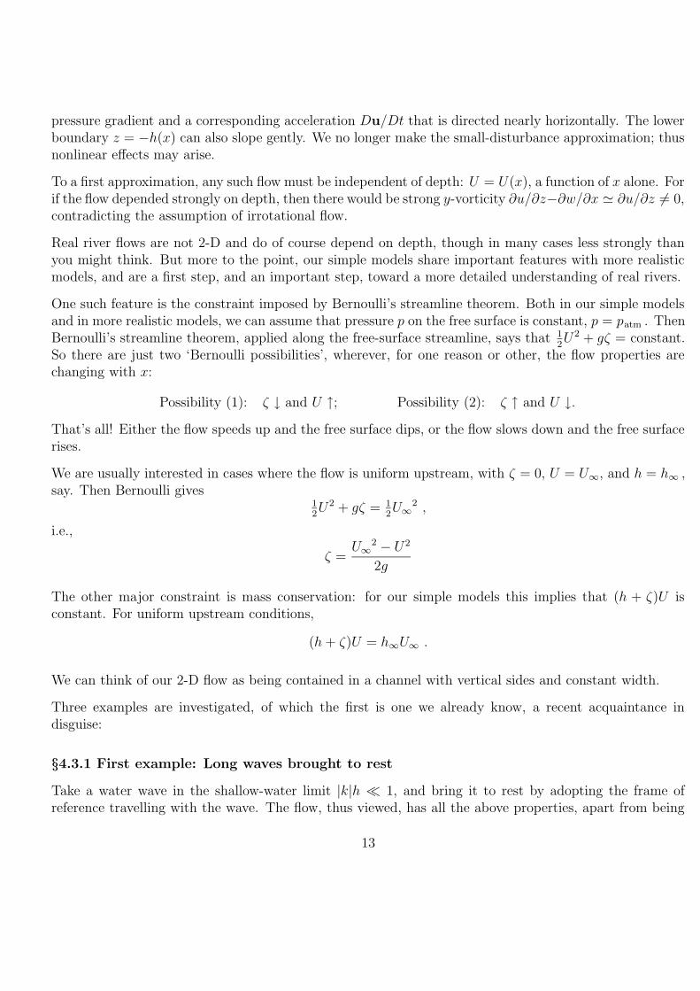
Note that this is valid for arbitrary x-dependence, not necessarily sinusoidal! It is enough for the xdependence to be ‘slow’ in the above sense. *This is related to the nondispersive property of waves in the shallow-

water limit: all Fourier components with |k|h ¿ 1 propagate with the same speed relative to the undisturbed fluid.* Inparticular, we can include the case of no disturbance upstream:

§4.3.2 Second example: Free-surface flow over a gentle bump

14

Does the free surface go up or down? You might think that it would always go down, because the flowmust speed up over the bump. This does occur, but only if U∞ is small enough.

We shall see that the free surface goes down, as it encounters the bump, if U∞ < (gh∞)1/2. It goes up ifU∞ > (gh∞)1/2.

As before,

12U2 + gζ = 1

2U∞

2 (Bernoulli on free-surface streamline) ,

(h + ζ)U = h∞U∞ (mass conservation) ,

two equations for two unknowns U and ζ. [We don’t use the momentum integral here, because we are notgiven, nor are we presently interested in, the horizontal force on the bump —*though the force is actually zero

in this case: d’Alembert’s paradox applies.*]

Eliminate ζ:

12U2 +

gh∞U∞

U= 1

2U∞

2 + gh

Use a graphical approach to see what this means in various cases. Denote by F (U) the function of Uappearing on left-hand side. Its graph is the curve sketched below. If we fix the value of gh∞U∞ (gravitytimes volume flux) then we have just one such curve. Solutions to the above equation, for given valuesof U∞ , gh∞ and gh , are given by intersections of the graph of F (U) with the horizontal straight line12U∞

2 + gh :

15

There is also a negative root (U times the above equation being a cubic): we ignore this as unphysical,representing negative U and negative thickness of the fluid layer.

Minimum of curve F (U) occurs at U = (gh∞U∞)1/3; U∞ falls to the right or left of this according asU∞

>< (gh∞)1/2.

These cases are called ‘supercritical’ and ‘subcritical’ respectively. The case U∞ = (gh∞)1/2 will be called‘critical’. In a subcritical flow, long waves can penetrate arbitrarily far upstream. In a supercriticalflow, no waves can penetrate upstream: all waves, even the longest, fastest-propagating waves, are sweptdownstream.

There are two real positive roots if and only if h > hmin ∀x , where

ghmin = 32(gh∞U∞)2/3 − 1

2U∞

2 .

If h < hmin (bump too tall), a flow of the kind we have assumed is not possible!

(What happens in reality, when h < hmin, is that the oncoming fluid will pile up on the upstream side of the bump, until h

does exceed hmin and locally steady flow does become possible. In the critical case, we have hmin = h∞, and the fluid will

begin to pile up even for an arbitrarily thin bump! This can be viewed as a case of resonant forcing of long waves.)

When h > hmin > 0, then, there are two positive roots:

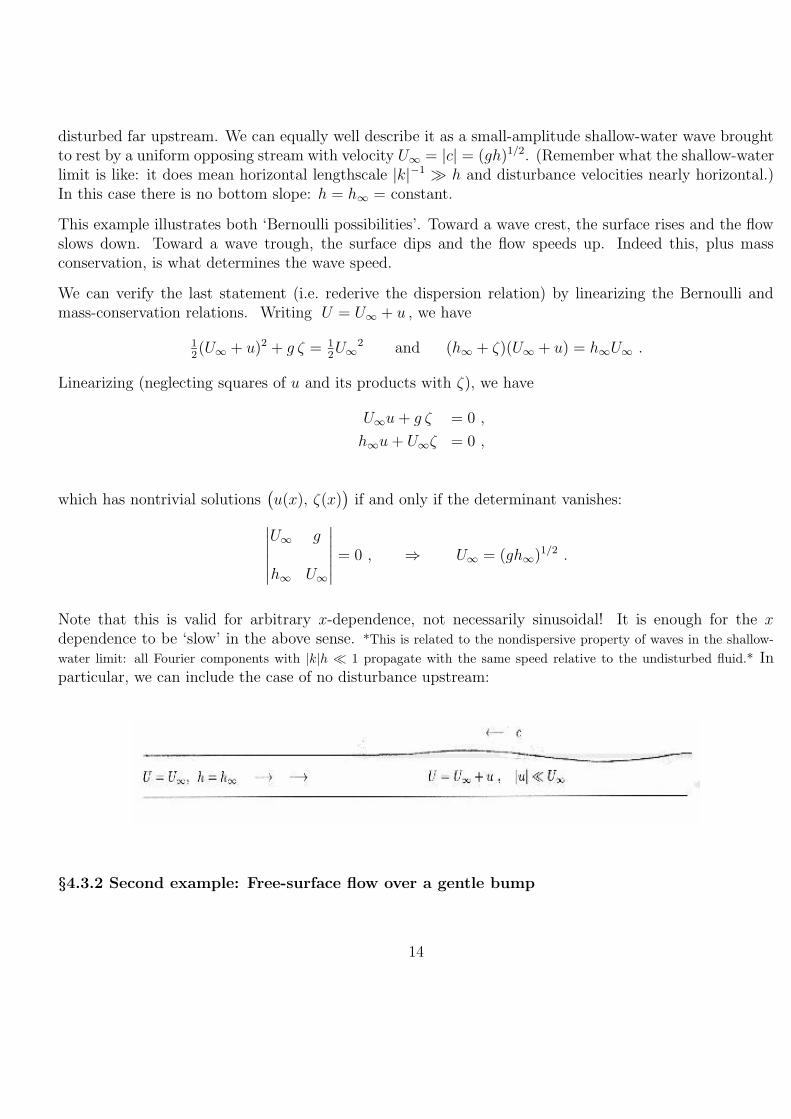
Smallest root: The oncoming flow is subcritical, and U is a

16

decreasing and ζ an increasing function of h. As the flowrides up the left-hand slope of the bump, h↓ , U ↑ and ζ ↓(free surface lowered); see arrow in sketch below (top):

Largest root: The oncoming flow is supercritical, and U isan increasing and ζ a decreasing function of h. As the flowrides up the left-hand slope of the bump, h↓ , U ↓ and ζ ↑(free surface raised); see arrow in sketch below (bottom):

§4.3.3 Third example: Flow out of a reservoir over a broad weir

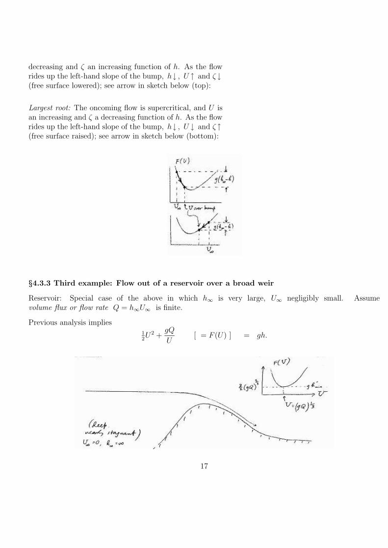
Reservoir: Special case of the above in which h∞ is very large, U∞ negligibly small. Assumevolume flux or flow rate Q = h∞U∞ is finite.

Previous analysis implies12U2 +

gQ

U[ = F (U) ] = gh.

17

In the reservoir we evidently start with the ‘smallest-root’ situation, the left-hand branch in the graphicalsolution above. (Infinitely slow flow is subcritical flow.) If we were to stay on this same branch, as wecross the weir, then surface would dip as the weir is crossed and then rise again. This is not what we seehappening at real weirs on real rivers; and it won’t happen unless someone were to force the downstreamwater level to rise by building a dam somewhere downstream.

So flow over a real weir — when it is acting as a weir, i.e. when downstream levels are low — must involvechanging the branch. The flow conditions must cross over from the left-hand (subcritical) to the right-hand(supercritical) branch as x varies across the weir.

We can change branch smoothly only if minimum h (at the crest of the weir), h′

min say, corresponds tominimum F (U) = 1

2U2 + gQU−1 (Q = h∞U∞). Hence

h′

min =3

2

(

Q2

g

)1/3

;

h′

min is a limiting case of the earlier hmin:

h′

min = g−1 limU∞→0

Q fixed

(

32(gh∞U∞)2/3 − 1

2U∞

2)

.

We know h′

min (the difference in elevation between the top of the weir and the level of the free surface inthe reservoir), and can therefore deduce Q, as

Q =

(

8

27g h

′

min3)1/2

.

In other words Q can be controlled by choice of h′

min, i.e. by choosing the height of the weir. Q is thereforecalled the ‘hydraulically controlled’ flow rate.

At the crest of the weir:

flow speed U = (23g h

′

min)1/2 ,

depth h + ζ = Q/U = 23h

′

min ,

free surface height ζ = − 13h

′

min .

Speed of long waves at crest of weir = U =(

g (23h

′

min))1/2

, so flow speed = wave speed. I.e., the flow atthe crest is critical.

The flow downstream is supercritical: no waves generated at positions downstream can penetrate upstream.Weirs and waterfalls send no disturbances back into the reservoir: unwary canoe enthusiasts watch out!

§4.4 Bores and hydraulic jumps

18

[‘bore’ as in ‘drill’, or ‘penetrate’. E.g. the famous ‘Severn bore’.]

Bores and hydraulic jumps are essentially the same thing viewed in different frames of reference: an abruptchange in velocity U and surface elevation ζ, propagating at constant speed, V say, relative to the fluidahead. Significant turbulent energy loss is involved in the transition region, as one might guess even fromcasual observation of these phenomena:

Turbulent energy loss in the transition region can be so strong, in fact, that Bernoulli cannot be used,even as a rough approximation.

Take the simplest case of a flat bottom (i.e. depth variations on lengthscale much larger than width of boreitself). There are no longer any horizontal forces, so we can now use the momentum integral to supplementmass conservation.

Apply mass conservation to fixed box containing the bore:

mass flux out = −d

dt( mass in box) ;

19

mass in (fixed) box is increasing. Therefore

−ρh2U2 = − V ρ(h2 − h1) ,

i.e.h2U2 = V (h2 − h1) .(1)

(Note that a segment of the box of length V δt changes from being ‘ahead’ of the bore to being ‘behind’the bore in time δt.)

Similarly apply momentum conservation to the box:

(force exerted by fluid in box on fluid outside)

+ (advective momentum flux out) = −d

dt(momentum in box):

∫ h1

0

p1(z)dz +

∫ h2

h1

patm dz −

∫ h2

0

p2(z)dz − ρh2U22 = − ρV h2U2 .

The pressure distributions p1(z) and p2(z) are hydrostatic and given by

p1(z) = patm + ρg(h1 − z) (0 < z < h1)

p2(z) = patm + ρg(h2 − z) (0 < z < h2)

Hence the momentum balance equation simplifies to

12gh2

1 −12gh2

2 − h2U22 = −V h2U2 .(2)

We now have two equations, with unknowns V and U2 (if regard h2 as given).

20

Eliminate U2:

12g(h2

1 − h22) = − h2

V (h2 − h1)

h2

V h1

h2

.

Hence

speed of bore V =

(

g(h1 + h2)h2

2h1

)1/2

,

flow speed behind bore U2 =h2 − h1

h2

V .

Note that V →(

gh1

)1/2if h2 → h1 , again checking consistency with small-amplitude wave theory,

whereas, at finite amplitude, h2 > h1 , we have

V >(

gh1

)1/2.

So the bore travels faster than, and will catch up with, any gravity waves ahead of it. But V − U2 =(

h1/h2

)

V <(

gh2

)1/2; i.e.

V < U2 +(

gh2

)1/2,

which says that waves upstream can catch up with the bore.

Exercise (last question on Ex. Sheet 3): Show that the rate of energy dissipation in the bore is positive ifh2 > h1; this must be so if the model is to be physically reasonable.

∼∼∼∼∼∼∼∼∼∼∼∼∼∼∼∼∼∼∼∼∼∼∼ End of notes ∼∼∼∼∼∼∼∼∼∼∼∼∼∼∼∼∼∼∼∼∼∼

21