COMPUTER VISION AND IMAGE UNDERSTANDING

Vol. 69, No. 1, January, pp. 23–37, 1998ARTICLE NO. IV960586

X Vision: A Portable Substrate for Real-Time Vision Applications

Gregory D. Hager and Kentaro Toyama

Department of Computer Science, Yale University, P.O. Box 208285, New Haven, Connecticut 06520E-mail: hager@cs.yale.edu, toyama@cs.yale.edu

Received January 15, 1996; accepted December 3, 1996

In the past several years, the speed of standard processors hasreached the point where interesting problems requiring visual track-ing can be carried out on standard workstations. However, relativelylittle attention has been devoted to developing visual tracking tech-nology in its own right. In this article, we describe X Vision, a mod-ular, portable framework for visual tracking. X Vision is designedto be a programming environment for real-time vision which pro-vides high performance on standard workstations outfitted witha simple digitizer. X Vision consists of a small set of image-leveltracking primitives, and a framework for combining tracking prim-itives to form complex tracking systems. Efficiency and robustnessare achieved by propagating geometric and temporal constraintsto the feature detection level, where image warping and special-ized image processing are combined to perform feature detectionquickly and robustly. Over the past several years, we have used XVision to construct several vision-based systems. We present someof these applications as an illustration of how useful, robust trackingsystems can be constructed by simple combinations of a few basicprimitives combined with the appropriate task-specific constraints.c© 1998 Academic Press

Key Words: real-time vision; feature-based visual tracking; vision-guided robotics.

1. INTRODUCTION

Real-time vision is an ideal source of feedback for systemsthat must interact dynamically with the world. Cameras are pas-sive and unobtrusive, they have a wide field of view, and theyprovide a means for accurately measuring the geometric prop-erties of physical objects. Potential applications for visual feed-back range from traditional problems such as robotic hand–eyecoordination and mobile robot navigation to more recent ar-eas of interest such as user interfaces, gesture recognition, andsurveillance.

One of the key problems in real-time vision is to track objectsof interest through a series of images. There are two generalclasses of image processing algorithms used for this task: full-field image processing followed by segmentation and match-ing and localized feature detection. Many tracking problemscan be solved using either approach, but it is clear that the

data-processing requirements for the solutions vary consider-ably. Full-frame algorithms such as optical flow calculation orregion segmentation tend to lead to data intensive processingwhich is performed off-line or which is accelerated using spe-cialized hardware (for a notable exception, see [36]). On theother hand, feature-based algorithms usually concentrate on spa-tially localized areas of the image. Since image processing islocal, high data bandwidth between the host and the digitizeris not needed. The amount of data that must be processed isalso relatively low and can be handled by sequential algorithmsoperating on standard computing hardware. Such systems arecost-effective and, since the tracking algorithms reside in soft-ware, extremely flexible and portable. Furthermore, as the speedof processors continues to increase, so does the complexityof the real-time vision applications that can be run on them.These advances anticipate the day when even full-frame appli-cations requiring moderate processing can be run on standardhardware.

Local feature tracking has already found wide applicability inthe vision and robotics literature. One of the most common ap-plications is determining structure from motion. Most often, thisresearch involves observation of line segments [12, 30, 43, 45,57], point features [41, 44], or both [14, 42], as they move in theimage. As with stereo vision research, a basic necessity for re-covering structure accurately is a solution to the correspondenceproblem: three-dimensional structure cannot be accurately de-termined without knowing which image features correspond tothe same physical point in successive image frames. In this sense,precise local feature tracking is essential for the accurate recov-ery of three-dimensional structure.

Robotic hand–eye applications also make heavy use of visualtracking. Robots often operate in environments rich with edges,corners, and textures, making feature-based tracking a naturalchoice for providing visual input. Specific applications includecalibration of cameras and robots [9, 28], visual-servoing andhand–eye coordination [10, 18, 25, 27, 56], mobile robot navi-gation and map-making [45, 55], pursuit of moving objects [10,26], grasping [1], and telerobotics [23]. Robotic applicationsmost often require the tracking of objects more complex thanline segments or point features, and they frequently require theability to track multiple objects. Thus, a tracking system for

231077-3142/98 $25.00

Copyright c© 1998 by Academic PressAll rights of reproduction in any form reserved.

24 HAGER AND TOYAMA

robotic applications must include a framework for composingsimple features to track objects such as rectangles, wheels, andgrippers in a variety of environments. At the same time, the factthat vision is in a servo loop implies that tracking must be fast,accurate, and highly reliable.

A third category of tracking applications are those which trackmodeled objects. Models may be anything from weak assump-tions about the form of the object as it projects to the cameraimage (e.g., contour trackers which assume simple, closed con-tours [8]) to full-fledged three-dimensional models with variableparameters (such as a model for an automobile which allows forturning wheels, opening doors). Automatic road-following hasbeen accomplished by tracking the edges of the road [34]. Var-ious snake-like trackers are used to track objects in 2D as theymove across the camera image [2, 8, 11, 29, 46, 49, 54]. Three-dimensional models, while more complex, allow for precise poseestimation [17, 31]. The key problem in model-based trackingis to integrate simple features into a consistent whole, both topredict the configuration of features in the future and to evaluatethe accuracy of any single feature.

While the list of tracking applications is long, the featuresused in these applications are variations on a very small set ofprimitives: “edgels” or line segments [12, 17, 30, 31, 43, 45, 49,57], corners based on line segments [23, 41], small patches oftexture [13], and easily detectable highlights [4, 39]. Althoughthe basic tracking principles for such simple features have beenknown for some time, experience has shown that tracking themis most effective when strong geometric, physical, and temporalconstraints from the surrounding task can be brought to bearon the tracking problem. In many cases, the natural abstractionis a multilevel framework where geometric constraints are im-posed “top-down” while geometric information about the worldis computed “bottom-up.”

Although tracking is a necessary function for most of the re-search listed above, it is generally not a focus of the work andis often solved in anad hocfashion for the purposes of a sin-gle demonstration. This has led to a proliferation of trackingtechniques which, although effective for particular experiments,are not practical solutions in general. Many tracking systems,for example, are only applied to prestored video sequences anddo not operate in real time [40]. The implicit assumption isthat speed will come, in time, with better technology (perhapsa reasonable assumption, but one which does not help thoseseeking real-time applications today). Other tracking systems re-quire specialized hardware [1], making it difficult for researcherswithout such resources to replicate results. Finally, most, ifnot all, existing tracking methodologies lack modularity andportability, forcing tracking modules to be reinvented for everyapplication.

Based on these observations, we believe that the availabilityof fast, portable, reconfigurable tracking system would greatlyaccelerate research requiring real-time vision tools. Just as theX Window system made graphical user interfaces a common fea-ture of desktop workstations, an analogous “X Vision” system

could make desktop visual tracking a standard tool in next gen-eration computing. We have constructed such a system, calledX Vision, both to study the science and art of visual tracking aswell as to conduct experiments utilizing visual feedback. Expe-rience from several teaching and research applications suggeststhat this system reduces the startup time for new vision appli-cations, makes real-time vision accessible to “nonexperts,” anddemonstrates that interesting research utilizing real-time visioncan be performed with minimal hardware.

This article describes the philosophy and design of X Vi-sion, focusing particularly on how geometric warping and geo-metric constraints are used to achieve high performance. Wealso present timing data for various tracking primitives and sev-eral demonstrations of X Vision-based systems. The remainderof the article is organized into four parts. Section 2 describesX Vision in some detail and Section 3 shows several exam-ples of its use. The final section suggests some of the futuredirections for this paradigm, and we include an appendix whichdiscusses some details of the software implementation.

2. TRACKING SYSTEM DESIGN ANDIMPLEMENTATION

It has often been said that “vision is inverse graphics.”X Vision embodies this analogy and carries it one step furtherby viewingvisual tracking as inverse animation. In particular,most graphics or animation systems implement a few simpleprimitives, e.g. lines and arcs, and define more complex ob-jects in terms of these primitives. So, for example, a polygonmay be decomposed into its polyhedral faces which are furtherdecomposed into constituent lines. Given an object–viewer re-lationship, these lines are projected into the screen coordinatesystem and displayed. A good graphics system makes definingthese types of geometric relationships simple and intuitive [15].

X Vision provides this functionalityand its converse. In ad-dition to stating how a complex object in a particular pose orconfiguration is decomposed into a list of primitive features,X Vision describes how the pose or attitude is computed fromthe locations of those primitives. More specifically, the system isorganized around a small set of image-level primitives referredto asbasic features. Each of these features is described in termsof a small set of parameters, referred to as astate vector, whichcompletely specify the feature’s position and appearance. Com-plex features or objects carry their own state vectors which arecomputed by defining functions or constraints on a collection ofsimpler state vectors. These complex features may themselvesparticipate in the construction of yet more complex features.Conversely, given the state vector of a complex feature, con-straints are imposed on the state of its constituent features andthe process recurses until image-level primitives are reached.The image-level primitives search for features in the neighbor-hood of their expected locations which produces a new statevector, and the cycle repeats.

X VISION: SUBSTRATE FOR REAL-TIME VISION 25

In addition to being efficient and modular, X Vision providesfacilities to simplify the embedding of vision into applications.In particular, X Vision incorporates data abstraction that disso-ciates information carried in the feature state from the trackingmechanism used to acquire it.

2.1. Image-Level Feature Tracking

The primitive feature tracking algorithms of X Vision areoptimized to be both accurate and efficient on scalar processors.These goals are met largely through two important attributes ofX Vision. First, any tracking primitive operates on a relativelysmall “region of interest” within the image. Tracking a featuremeans that the region of interest maintains a fixed, predefinedrelationship to the feature. In X Vision, a region of interest isreferred to as awindow. Fundamentally, the goal of low-levelprocessing is to process the pixels within a window using aminimal number of addressing operations, bus transfer cycles,and arithmetic operations.

The second key idea is to employimage warpingto geomet-rically transform windows so that image features appear in acanonical configuration. Subsequent processing of the warpedwindow can then be simplified by assuming the feature is inor near this canonical configuration. As a result, the imageprocessing algorithms used in feature-tracking can focus onthe problem of accurateconfiguration adjustmentrather thangeneral-purpose feature detection. For example, consider lo-cating a straight edge segment with approximately known ori-entation within an image region. Traditional feature detectionmethods utilize one or more convolutions, thresholding, andfeature aggregation algorithms to detect edge segments. Thisis followed by a matching phase which utilizes orientation, seg-ment length, and other cues to choose the segment which cor-responds to the target [5]. Because the orientation and linearityconstraints appear late in the detection process, such methodsspend a large amount of time performing general purpose edgedetection which in turn generates large amounts of data thatmust then be analyzed in the subsequent match phase. A moreeffective approach, as described in Section 2.1.2, is to exploitthese constraints at the outset by utilizing a detector tuned forstraight edges.

An additional advantage to warping-based algorithms is thatthey separate the “change of coordinates” needed to rectify afeature from the image processing used to detect it. On onehand, the same type of coordinate transforms, e.g., rigid trans-formations, occur repeatedly, so the same warping primitivescan be reused. On the other hand, various types of warping canbe used to normalize features so that the same accelerated im-age processing can be applied over and over again. For example,quadratic warping could be used to locally “straighten” a curvededge so that an optimized straight edge detection strategy canbe applied.

The low-level features currently available in X Vision in-clude solid or broken contrast edges detected using several vari-ations on standard edge-detection, general grey-scale patterns

tracked using SSD (sum-of-squared differences) methods [3,47], and a variety of color and motion-based primitives usedfor initial detection of objects and subsequent match disam-biguation [51]. The remainder of this section describes howedge tracking and correlation-based tracking have been incor-porated into X Vision. In the sequel, all reported timing fig-ures were taken on an SGI Indy workstation equipped with a175 MHz R4400 SC processor and an SGI VINO digitizingsystem. Nearly equivalent results have been obtained for a SunSparc 20 equipped with a 70 MHz supersparc processor and for a120 MHz Pentium microprocessor, both with standard digitizersand cameras.

2.1.1. Warping In the remainder of this article, we defineacquiringa window to be the transferandwarping of the win-dow’s pixels. The algorithms described in this article use rigidand affine warping of rectangular image regions. The warpingalgorithms are based on the observation that a positive-definitelinear transformationA can be written as a product of an upper-triangular matrixU and a rotation matrixR(θ ) as

A = UR(θ ) =[

sx γ

0 sy

] [cos(θ ) −sin(θ )sin(θ ) cos(θ )

]. (1)

The implementation of image warping mirrors this factor-ization. First, a rotated rectangular area is acquired using analgorithm closely related to Bresenham algorithms for fast linerendering [15]. The resulting buffer can be subsequently scaledand sheared using an optimized bilinear interpolation algorithm.The former is relatively inexpensive, requiring about two ad-ditions per pixel to implement. The latter is more expensive,requiring three multiplies and six additions per pixel in our im-plementation. The initial acquisition is also parameterized by asampling factor, making it possible to acquire decimated imagesat no additional cost. The warping algorithm supports reductionof resolution by averaging neighborhoods of pixels at a costof one addition and 1/r multiplies per pixel for reduction bya factor ofr . Figure 1 shows the time consumed by the threestages of warping (rotation, scale, and resolution reduction) onvarious size regions and shows the effective time consumed foraffine warping followed by resolution reduction to three differ-ent scales.

For the purposes of later discussion, we denote an image re-gion acquired at timet asR(t). The region containing the en-tire camera image at timet is writtenI(t). Warping operatorsoperate on image regions to produce new regions. We writeR(t) = warp rot (I(t); d, θ ) to denote the acquisition of an im-age region centered atd = (x, y)t and rotated byθ . Likewise,using the definition ofU above,R′(t) = warp ss (R(t); U) de-notes scaling the image regionR(t) by sx andsy and shearingby γ . Affine warping is defined as

warp aff (I(t); A, d) = warp ss (warp rot (I(t); d, θ ); U),(2)

whereA is as in (1).

26 HAGER AND TOYAMA

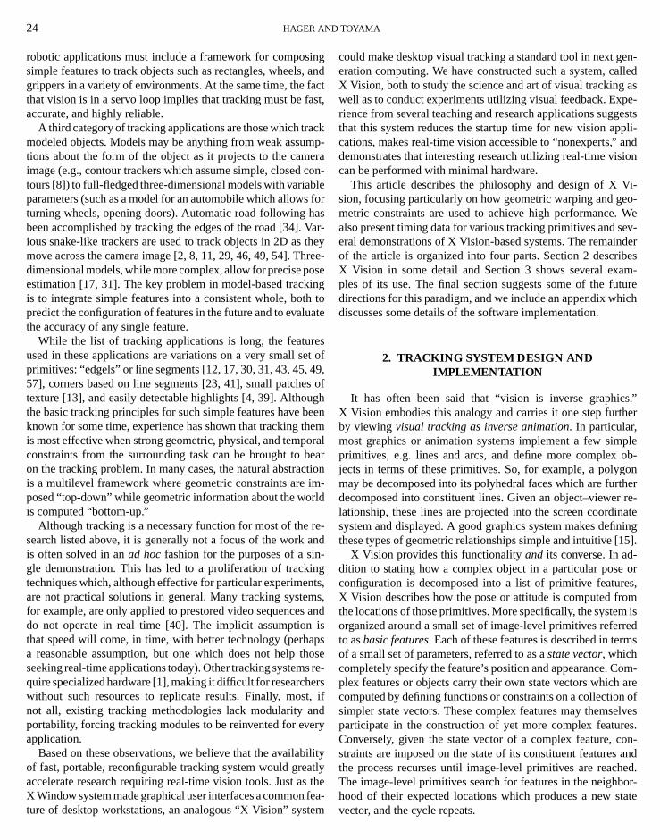
FIG. 1. The time in milliseconds consumed by image warping for varioussize regions. The first two lines show the time for each of the warping stages.The time taken for scale and shear varies with the amount of scaling done; thetimings in the second row are for scaling the input image by a factor of 1/1.1.The third and fourth lines show the time taken for reducing image resolution byfactors of 2 and 4. The final lines show the time needed for affine warping atvarious scales, based on the component times.

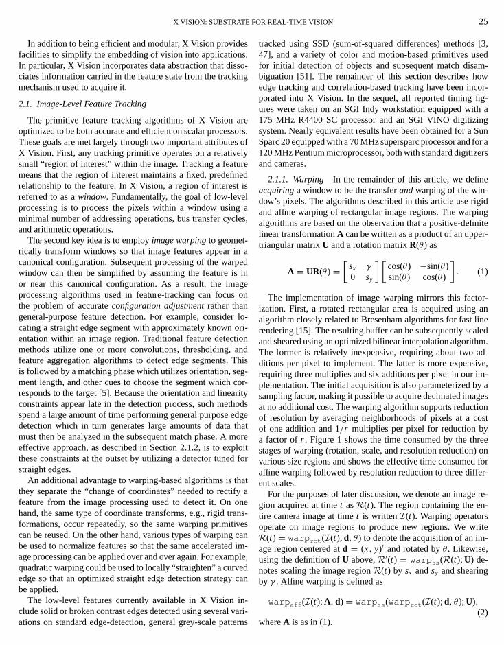
2.1.2. Edges X Vision provides a tracking mechanism forlinear edge segments of arbitrary length (Fig. 2). The state of anedge segment consists of its position,d = (x, y)t , and orienta-tion,θ , in framebuffer coordinates as well as its filter responser .Given prior state informationL t = (xt , yt , θt , rt )t , we can writethe feature tracking cycle for the edge state computation at timet + τ schematically as

L t+τ = L t + Edge(warp rot (I(t + τ ); xt , yt , θt ); L t ). (3)

The edge tracking procedure can be divided into two stages:feature detection and state updating. In the detection stage, rota-tional image warping is used to acquire a window which, if theprior estimate is correct, leads to an edge which is vertical withinthe warped window. Detecting a straight, vertical contrast stepedge can be implemented by convolving each row of the win-dow with a derivative-based kernel and averaging the resultingresponse curves by summing down the columns of the window.Finding the maximum value of this response function localizesthe edge. Performance can be improved by noting that the order

FIG. 2. Close-up of tracking windows at two time points. Left, timeti , where the edge tracking algorithm has computed the correct warp parameters to make anedge appear vertical (the “setpoint”). Right, the edge acquired at timeti+1. The warp parameters computed forti were used to acquire the image, but the underlyingedge has changed orientation. Figure 3 shows how the new orientation is computed.

of the convolution and summation steps can be commuted. Thus,in ann×m window, edge localization with a convolution maskof width k can be performed with justm× (n+k) additions andmkmultiplications. We, in fact, often use an IR filter composedof a series of−1s, one or more 0s, and a series of+1s which canbe implemented using onlym× (n+ 4) additions. We note thatthis is significantly cheaper than using, for example, steerablefilters for this purpose [16].

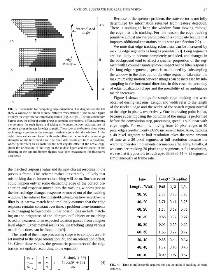
The detection scheme described above requires orientationinformation to function correctly. If this information cannot besupplied from “higher-level” geometric constraints, it is esti-mated as follows (refer to Fig. 3). As the orientation of theacquisition window rotates relative to the edge, the responseof the filter drops sharply. Thus, edge orientation can be com-puted by sampling at several orientations and interpolating theresponses to locate the direction of maximum response. How-ever, implementing this scheme directly would be wasteful be-cause the acquisition windows would overlap, causing manypixels to be transferred and warped three times. To avoid thisoverhead, an expanded window at the predicted orientation isacquired, and the summation step is repeated three times: oncealong the columns, and once along two diagonal paths at a smallangular offset from vertical. This effectively approximates rota-tion by image shear, a well-known technique in graphics [15].Quadratic interpolation of the maximum of the three curves isused to estimate the orientation of the underlying edge. In theideal case, if the convolution template is symmetric and the re-sponse function after superposition is unimodal, the horizontaldisplacement of the edge should agree between all three filters.In practice, the estimate of edge location will be biased. For thisreason, edge location is computed as the weighted average ofthe edge location of all three peaks.

Even though the edge detector described above is quite selec-tive, as the edge segment moves through clutter, we can expectmultiple local maxima to appear in the convolution output. Thisis a well-known and unavoidable problem for which many so-lutions have been proposed [38]. By default, X Vision declaresa match if and only if a unique local maximum exists withinan interval about the response value stored in the state. Thematch interval is chosen as a fraction of the difference between

X VISION: SUBSTRATE FOR REAL-TIME VISION 27

FIG. 3. Schematic for computing edge orientation. The diagrams on the leftshow a window of pixels at three different “orientations.” The middle figuredisplays the edge after a warped acquisition (Fig. 2, right). The top and bottomfigures show the effect of shifting rows to simulate orientational offset. Summingthe columns for each figure and taking differences between adjacent sets ofcolumns gives estimates for edge strength. The arrows at the bottom show whereeach image experiences the strongest vertical edge within the window. At theright, these values are plotted with angle offset on the vertical axis and edgestrengths on the horizontal axis. The three data points are fit to a quadratic,whose peak offers an estimate for the best angular offset of the actual edge.(Both the orientation of the edge in the middle figure and the extent of theshearing in the top and bottom figures have been exaggerated for illustrativepurposes.)

the matched response value and its next closest response in theprevious frame. This scheme makes it extremely unlikely thatmistracking due to incorrect matching will occur. Such an eventcould happen only if some distracting edge of the correct ori-entation and response moved into the tracking window just asthe desired edge changed response or moved out of the trackingwindow. The value of the threshold determines how selective thefilter is. A narrow match band implicitly assumes that the edgeresponse remains constant over time, a problem in environmentswith changing backgrounds. Other possibilities include match-ing on the brightness of the “foreground” object or matchingbased on nearness to an expected location passed from a higherlevel object. Experimental results on line tracking using variousmatch functions can be found in [49].

The result of the image processing stage is to compute an off-set normal to the edge orientation,δt , and an orientation offset,δθ . Given these values, the geometric parameters of the edgetracker are updated according to the equation xt+τ

yt+τθt+τ

= xt

yt

θt

+−δt sin(θt + δθ )δt cos(θt + δθ )

δθ

(4)

Because of the aperture problem, the state vector is not fullydetermined by information returned from feature detection.There is nothing to keep the window from moving “along”the edge that it is tracking. For this reason, the edge trackingprimitive almost always participates in a composite feature thatimposes additional constraints on its state (see Section 2.2).

We note that edge tracking robustness can be increased bymaking edge segments as long as possible [50]. Long segmentsare less likely to become completely occluded, and changes inthe background tend to affect a smaller proportion of the seg-ment with a commensurately lower impact on the filter response.On long edge segments, speed is maintained by subsamplingthe window in the direction of the edge segment. Likewise, themaximum edge motion between images can be increased by sub-sampling in the horizontal direction. In this case, the accuracyof edge localization drops and the possibility of an ambiguousmatch increases.

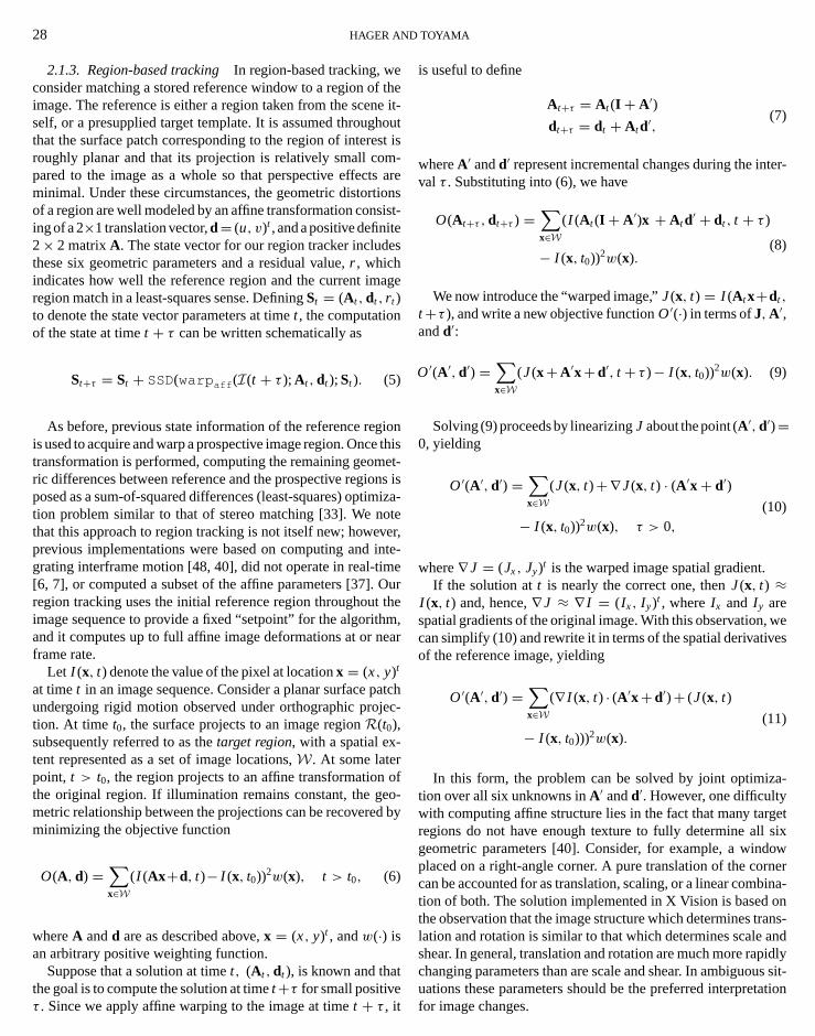
Figure 4 shows timings for simple edge tracking that wereobtained during test runs. Length and width refer to the lengthof the tracked edge and the width of the search region normalto the edge in pixels, respectively. One interesting point is that,because superimposing the columns of the image is performedbefore the convolution step, processing speed is sublinear withedge length. For example, moving from 20 pixel edges to 40pixel edges results in only a 65% increase in time. Also, trackinga 40 pixel segment at half resolution takes the same amountof time as a 20 pixel segment at full resolution because thewarping operator implements decimation efficiently. Finally, ifwe consider tracking 20 pixel edge segments at full resolution,we see that it is possible to track up to 33.33/0.44≈ 85 segmentssimultaneously at frame rate.

FIG. 4. Time in milliseconds required for one iteration of tracking an edgesegment.

28 HAGER AND TOYAMA

2.1.3. Region-based trackingIn region-based tracking, weconsider matching a stored reference window to a region of theimage. The reference is either a region taken from the scene it-self, or a presupplied target template. It is assumed throughoutthat the surface patch corresponding to the region of interest isroughly planar and that its projection is relatively small com-pared to the image as a whole so that perspective effects areminimal. Under these circumstances, the geometric distortionsof a region are well modeled by an affine transformation consist-ing of a 2×1 translation vector,d= (u, v)t , and a positive definite2× 2 matrixA. The state vector for our region tracker includesthese six geometric parameters and a residual value,r , whichindicates how well the reference region and the current imageregion match in a least-squares sense. DefiningSt = (At , dt , rt )to denote the state vector parameters at timet , the computationof the state at timet + τ can be written schematically as

St+τ = St + SSD(warp aff (I(t + τ ); At , dt ); St ). (5)

As before, previous state information of the reference regionis used to acquire and warp a prospective image region. Once thistransformation is performed, computing the remaining geomet-ric differences between reference and the prospective regions isposed as a sum-of-squared differences (least-squares) optimiza-tion problem similar to that of stereo matching [33]. We notethat this approach to region tracking is not itself new; however,previous implementations were based on computing and inte-grating interframe motion [48, 40], did not operate in real-time[6, 7], or computed a subset of the affine parameters [37]. Ourregion tracking uses the initial reference region throughout theimage sequence to provide a fixed “setpoint” for the algorithm,and it computes up to full affine image deformations at or nearframe rate.

Let I (x, t) denote the value of the pixel at locationx = (x, y)t

at timet in an image sequence. Consider a planar surface patchundergoing rigid motion observed under orthographic projec-tion. At time t0, the surface projects to an image regionR(t0),subsequently referred to as thetarget region, with a spatial ex-tent represented as a set of image locations,W. At some laterpoint, t > t0, the region projects to an affine transformation ofthe original region. If illumination remains constant, the geo-metric relationship between the projections can be recovered byminimizing the objective function

O(A, d) =∑x∈W

(I (Ax+d, t)− I (x, t0))2w(x), t > t0, (6)

whereA andd are as described above,x = (x, y)t , andw(·) isan arbitrary positive weighting function.

Suppose that a solution at timet, (At , dt ), is known and thatthe goal is to compute the solution at timet+τ for small positiveτ . Since we apply affine warping to the image at timet + τ , it

is useful to define

At+τ = At (I + A′)dt+τ = dt + Atd′,

(7)

whereA′ andd′ represent incremental changes during the inter-val τ . Substituting into (6), we have

O(At+τ , dt+τ ) =∑x∈W

(I (At (I + A′)x + Atd′ + dt , t + τ )

(8)− I (x, t0))2w(x).

We now introduce the “warped image,”J(x, t) = I (Atx+dt ,

t+τ ), and write a new objective functionO′(·) in terms ofJ,A′,andd′:

O′(A′, d′) =∑x∈W

(J(x+A′x+ d′, t + τ )− I (x, t0))2w(x). (9)

Solving (9) proceeds by linearizingJ about the point (A′, d′)=0, yielding

O′(A′, d′) =∑x∈W

(J(x, t)+∇ J(x, t) · (A′x+ d′)

− I (x, t0))2w(x), τ > 0,(10)

where∇ J = (Jx, Jy)t is the warped image spatial gradient.If the solution att is nearly the correct one, thenJ(x, t) ≈

I (x, t) and, hence,∇ J ≈ ∇ I = (Ix, I y)t , whereIx and I y arespatial gradients of the original image. With this observation, wecan simplify (10) and rewrite it in terms of the spatial derivativesof the reference image, yielding

O′(A′, d′) =∑x∈W

(∇ I (x, t) · (A′x+ d′)+ (J(x, t)

− I (x, t0)))2w(x).(11)

In this form, the problem can be solved by joint optimiza-tion over all six unknowns inA′ andd′. However, one difficultywith computing affine structure lies in the fact that many targetregions do not have enough texture to fully determine all sixgeometric parameters [40]. Consider, for example, a windowplaced on a right-angle corner. A pure translation of the cornercan be accounted for as translation, scaling, or a linear combina-tion of both. The solution implemented in X Vision is based onthe observation that the image structure which determines trans-lation and rotation is similar to that which determines scale andshear. In general, translation and rotation are much more rapidlychanging parameters than are scale and shear. In ambiguous sit-uations these parameters should be the preferred interpretationfor image changes.

X VISION: SUBSTRATE FOR REAL-TIME VISION 29

To implement this solution, we decomposeA′ into a differen-tial rotation and an upper triangular matrix:

A′ =[

0 α

−α 0

]+[

sx γ

0 sy

](12)

and solve for two parameter groups, (d, α) and (sx, sy, γ ), se-quentially. This establishes preferences for interpreting imagechanges (the result being that some image perturbations resultin short detours in the state space before arriving at a final stateestimate). Although less accurate than a simultaneous solution,the small amount of distortion between temporally adjacent im-ages makes this solution method sufficiently precise for mostapplications.

We first solve for translation and rotation. For an image loca-tion x = (x, y)t we define

gx(x) = Ix(x, t0)√w(x)

gy(x) = I y(x, t0)√w(x)

gr (x) = (y Ix(x, t0)− x Iy(x, t0))√w(x)

h0(x) = (J(x, t)− I (x, t0))√w(x),

(13)

and the linear system for computing translation and rotation is

∑x∈W

gxgx gxgy gxgr

gygx gygy gygr

gr gx gr gy gr gr

[ dα

]=∑x∈W

h0gx

h0gy

h0gr

. (14)

Since the spatial derivatives are only computed using the orig-inal reference image,gx, gy, andgr are constant over time, sothose values and the inverse of the matrix on the left-hand sideof (14) can be computed off-line.

Onced andα are known, the least squares residual value iscomputed as

h1(x) = h0(x)− gx(x)u− gy(x)v − gr (x)α. (15)

If the image distortion arises from pure translation and nonoise is present, then we expect thath1(x) = 0 after this step.Any remaining residual can be attributed to geometric distortionsin the second group of parameters, linearization error, or noise.To recover scale changes and shear, we define for an imagelocationx = (x, y)t

gsx(x) = xgx(x),

gsy(x) = ygy(x),

gγ (x) = ygx(x),

(16)

and the linear system for computing scaling and shear parameters

is

∑x∈W

gsxgsx gsxgsy gsxgγgsygsx gsygsy gsygγgγ gsx gγ gsy gγ gγ

sx

sy

γ

=∑x∈W

h1gsx

h1gsy

h1gγ

.(17)

As before,gsx, gsy and gγ can be precomputed as can theinverse of the matrix on the left hand side. The residual is

h2(x) = h1(x)− gsx(x)sx − gsy(x)sy − gr (x)γ. (18)

After all relevant stages of processing have been completed,

r =√∑

x∈W h2(x)2

|W| (19)

is stored as the match value of the state vector.One potential problem with this approach is that the bright-

ness and contrast of the target are unlikely to remain constantwhich may bias the results of the optimization. The solution is tonormalize images to have zero first moment and unit second mo-ment. We note that with these modifications, solving (6) for rigidmotions (translation and rotation) is equivalent to maximizingnormalized correlation [24]. Extensions to the SSD-based re-gion tracking paradigm for more complex lighting models canbe found in [21].

Another problem is that the image gradients are only locallyvalid. In order to guarantee tracking of motions larger than a frac-tion of a pixel, these calculations must be carried out at varyinglevels of resolution. For this reason, a software reduction of reso-lution is carried out at the time of window acquisition. All of theabove calculations except for image scaling are computed at thereduced resolution, and the estimated motion values are appro-priately rescaled. The tracking algorithm changes the resolutionadaptively based on image motion. If the computed motion valuefor either component ofd′ exceeds 0.25, the resolution for thesubsequent step is halved. If the interframe motion is less than0.1, the resolution is doubled. This leads to a fast algorithm fortracking fast motions and a slower but more accurate algorithmfor tracking slower motions.

If we consider the complexity of tracking in terms of arith-metic operations on pixels (asymptotically, these calculationsdominate the other operations needed to solve the linear sys-tem), we see that there is a fixed overhead of one differenceand multiply to computeh0. Each parameter computed requiresan additional multiply and addition per pixel. Computing theresidual values consumes a multiply and addition per pixel perparameter value. In addition to parameter estimation, the initialbrightness and contrast compensation consume three additionsand two multiplies per pixel. Thus, to compute the algorithm ata resolutiond requires 15/d2 multiplies and 1+16/d2 additionsper pixel (neglecting warping costs). It is interesting to note thatat a reduction factor ofd = 4, the algorithm compares favorablywith edge detection on comparably-sized regions.

30 HAGER AND TOYAMA

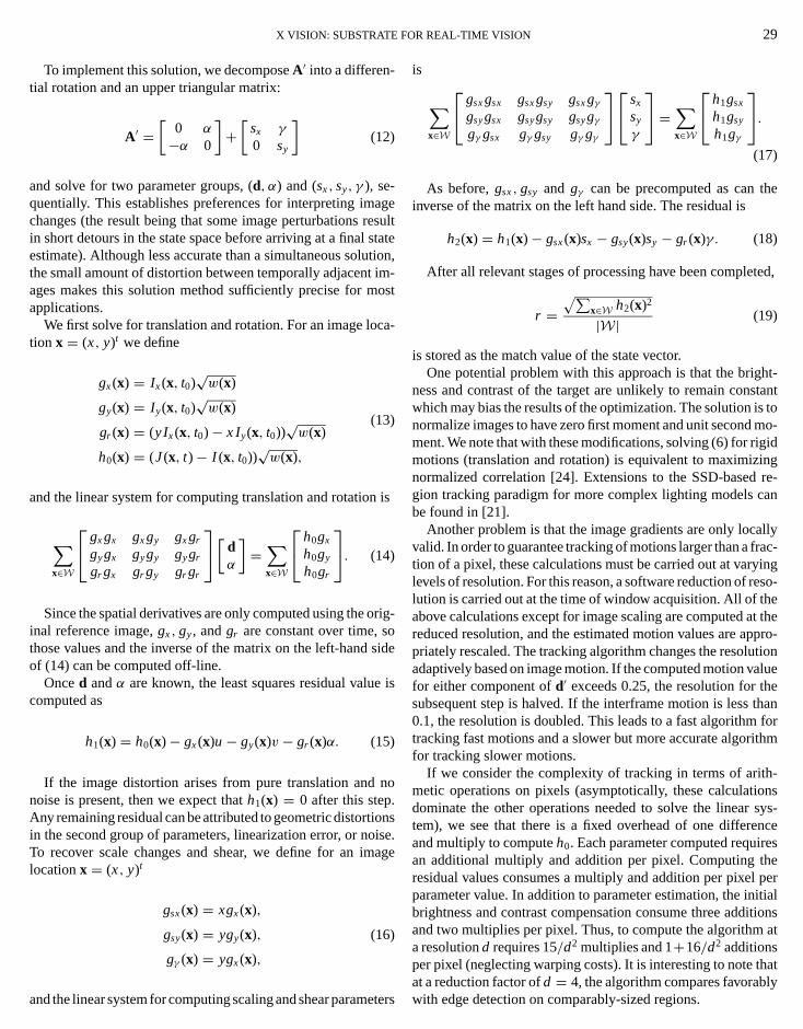
FIG. 5. The time in milliseconds consumed by one cycle of tracking for variousinstantiations of the SSD tracker. The first row shows the timings for rigid motion(translation and rotation), and the second row shows the time for full affinedeformations.

To get a sense of the time consumed by these operations,several test cases are shown in Fig. 5. The first row shows thetime needed to track rigid motions (translation and rotation) andthe second shows the time taken for tracking with full affinedeformations. The times include both warping and parameterestimation; the times given in Fig. 1 can be subtracted to deter-mine the time needed to estimate parameter values. In particular,it is important to note that, because the time consumed by affinewarping is nearly constant with respect to resolution, parameterestimation tends to dominate the computation for half and fullresolution tracking, while image warping tends to dominate thecomputation for lower resolution tracking. With the exceptionof 100× 100 images at half resolution, all updates require lessthan one frame time (33.33 ms) to compute. Comparing withFig. 4, we observe that the time needed to track a 40×40 regionat one-fourth resolution is nearly equivalent to that needed totrack a comparably-sized edge segment as expected from thecomplexity analysis given above.

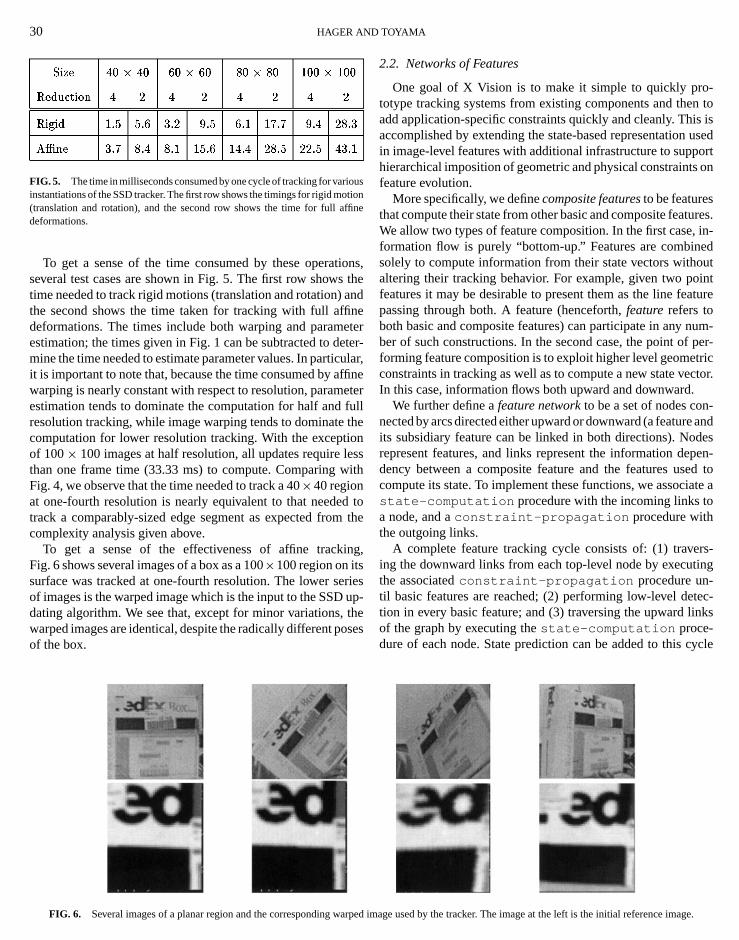
To get a sense of the effectiveness of affine tracking,Fig. 6 shows several images of a box as a 100×100 region on itssurface was tracked at one-fourth resolution. The lower seriesof images is the warped image which is the input to the SSD up-dating algorithm. We see that, except for minor variations, thewarped images are identical, despite the radically different posesof the box.

FIG. 6. Several images of a planar region and the corresponding warped image used by the tracker. The image at the left is the initial reference image.

2.2. Networks of Features

One goal of X Vision is to make it simple to quickly pro-totype tracking systems from existing components and then toadd application-specific constraints quickly and cleanly. This isaccomplished by extending the state-based representation usedin image-level features with additional infrastructure to supporthierarchical imposition of geometric and physical constraints onfeature evolution.

More specifically, we definecomposite featuresto be featuresthat compute their state from other basic and composite features.We allow two types of feature composition. In the first case, in-formation flow is purely “bottom-up.” Features are combinedsolely to compute information from their state vectors withoutaltering their tracking behavior. For example, given two pointfeatures it may be desirable to present them as the line featurepassing through both. A feature (henceforth,featurerefers toboth basic and composite features) can participate in any num-ber of such constructions. In the second case, the point of per-forming feature composition is to exploit higher level geometricconstraints in tracking as well as to compute a new state vector.In this case, information flows both upward and downward.

We further define afeature networkto be a set of nodes con-nected by arcs directed either upward or downward (a feature andits subsidiary feature can be linked in both directions). Nodesrepresent features, and links represent the information depen-dency between a composite feature and the features used tocompute its state. To implement these functions, we associate astate-computation procedure with the incoming links toa node, and aconstraint-propagation procedure withthe outgoing links.

A complete feature tracking cycle consists of: (1) travers-ing the downward links from each top-level node by executingthe associatedconstraint-propagation procedure un-til basic features are reached; (2) performing low-level detec-tion in every basic feature; and (3) traversing the upward linksof the graph by executing thestate-computation proce-dure of each node. State prediction can be added to this cycle

X VISION: SUBSTRATE FOR REAL-TIME VISION 31

by including it in the downward constraint propagation phase.Thus, a feature tracking system is completely characterized bythe topology of the network, the identity of the basic features,and the state computation and constraint propagation functionsfor each nonbasic feature node.

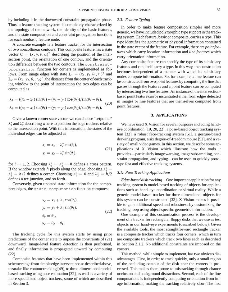
A concrete example is a feature tracker for the intersectionof two noncollinear contours. This composite feature has a statevectorC = (x, y, θ, α)T describing the position of the inter-section point, the orientation of one contour, and the orienta-tion difference between the two contours. Theconstraint-propagation function for corners is implemented as fol-lows. From image edges with stateL1 = (x1, y1, θ1, r1)T andL2 = (x2, y2, θ2, r2)T , the distance from the center of each track-ing window to the point of intersection the two edges can becomputed as

λ1 = ((x2− x1) sin(θ2)− (y2− y1) cos(θ2))/sin(θ2− θ1),(20)

λ2 = ((x2− x1) sin(θ1)− (y2− y1) cos(θ1))/sin(θ2− θ1).

Given a known corner state vector, we can choose “setpoints”λ∗1 andλ∗2 describing where to position the edge trackers relativeto the intersection point. With this information, the states of theindividual edges can be adjusted as

xi = xc − λ∗i cos(θi ),(21)

yi = yc − λ∗i sin(θi ),

for i = 1, 2. Choosingλ∗1 = λ∗2 = 0 defines a cross pattern.If the window extendsh pixels along the edge, choosingλ∗1 =λ∗2 = h/2 defines a corner. Choosingλ∗1 = 0 andλ∗2 = h/2defines a tee junction, and so forth.

Conversely, given updated state information for the compo-nent edges, thestate-computation function computes:

xc = x1+ λ1 cos(θ1),

yc = y1+ λ1 sin(θ1),(22)

θc = θ1,

αc = θ2− θ1.

The tracking cycle for this system starts by using priorpredictions of the corner state to impose the constraints of (21)downward. Image-level feature detection is then performed,and finally information is propagated upward by computing(22).

Composite features that have been implemented within thisscheme range from simple edge intersections as described above,to snake-like contour tracking [49], to three-dimensional model-based tracking using pose estimation [32], as well as a variety ofmore specialized object trackers, some of which are describedin Section 3.

2.3. Feature Typing

In order to make feature composition simpler and moregeneric, we have included polymorphic type support in the track-ing system. Each feature, basic or composite, carries a type. Thistype identifies the geometric or physical information containedin the state vector of the feature. For example, there arepoint fea-tureswhich carry location information andline featureswhichcarry orientation information.

Any composite feature can specify the type of its subsidiaryfeatures and can itself carry a type. In this way, the constructionbecomes independent of a manner with which its subsidiarynodes compute information. So, for example, a line feature canbe constructed from two point features by computing the line thatpasses through the features and a point feature can be computedby intersecting two line features. An instance of the intersection-based point feature can be instantiated either from edges detectedin images or line features that are themselves computed frompoint features.

3. APPLICATIONS

We have used X Vision for several purposes including hand–eye coordination [19, 20, 22], a pose-based object tracking sys-tem [32], a robust face-tracking system [51], a gesture-baseddrawing program, a six degree-of-freedom mouse [52], and a va-riety of small video games. In this section, we describe some ap-plications of X Vision which illustrate how the tools itprovides—particularly image warping, image subsampling, con-straint propagation, and typing—can be used to quickly proto-type fast and effective tracking systems.

3.1. Pure Tracking Applications

Edge-based disk trackingOne important application for anytracking system is model-based tracking of objects for applica-tions such as hand–eye coordination or virtual reality. While ageneric model-based tracker for three-dimensional objects forthis system can be constructed [32], X Vision makes it possi-ble to gain additional speed and robustness by customizing thetracking loop using object-specific geometric information.

One example of this customization process is the develop-ment of a tracker for rectangular floppy disks that we use as testobjects in our hand–eye experiments (described below). Giventhe available tools, the most straightforward rectangle trackeris a composite tracker which tracks four corners, which in turnare composite trackers which track two lines each as describedin Section 2.1.2. No additional constraints are imposed on thecorners.

This method, while simple to implement, has two obvious dis-advantages. First, in order to track quickly, only a small regionof the occluding contour of the disk near the corners is pro-cessed. This makes them prone to mistracking through chanceocclusion and background distractions. Second, each of the linecomputations is independently computing orientation from im-age information, making the tracking relatively slow. The first

32 HAGER AND TOYAMA

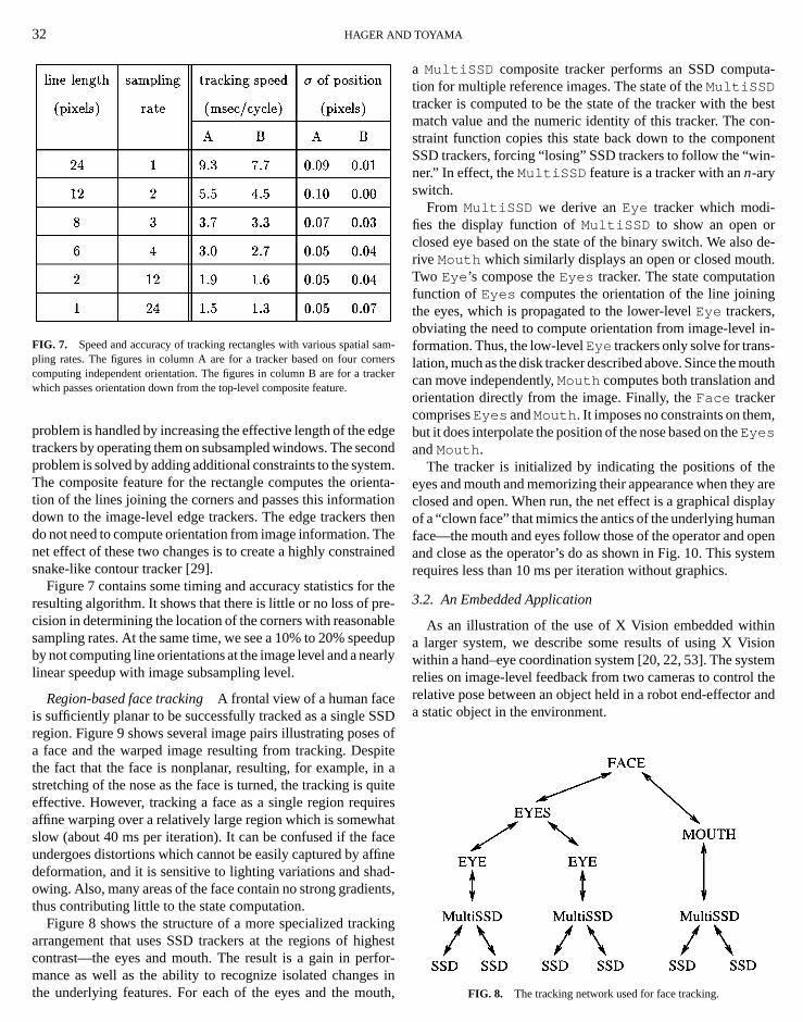
FIG. 7. Speed and accuracy of tracking rectangles with various spatial sam-pling rates. The figures in column A are for a tracker based on four cornerscomputing independent orientation. The figures in column B are for a trackerwhich passes orientation down from the top-level composite feature.

problem is handled by increasing the effective length of the edgetrackers by operating them on subsampled windows. The secondproblem is solved by adding additional constraints to the system.The composite feature for the rectangle computes the orienta-tion of the lines joining the corners and passes this informationdown to the image-level edge trackers. The edge trackers thendo not need to compute orientation from image information. Thenet effect of these two changes is to create a highly constrainedsnake-like contour tracker [29].

Figure 7 contains some timing and accuracy statistics for theresulting algorithm. It shows that there is little or no loss of pre-cision in determining the location of the corners with reasonablesampling rates. At the same time, we see a 10% to 20% speedupby not computing line orientations at the image level and a nearlylinear speedup with image subsampling level.

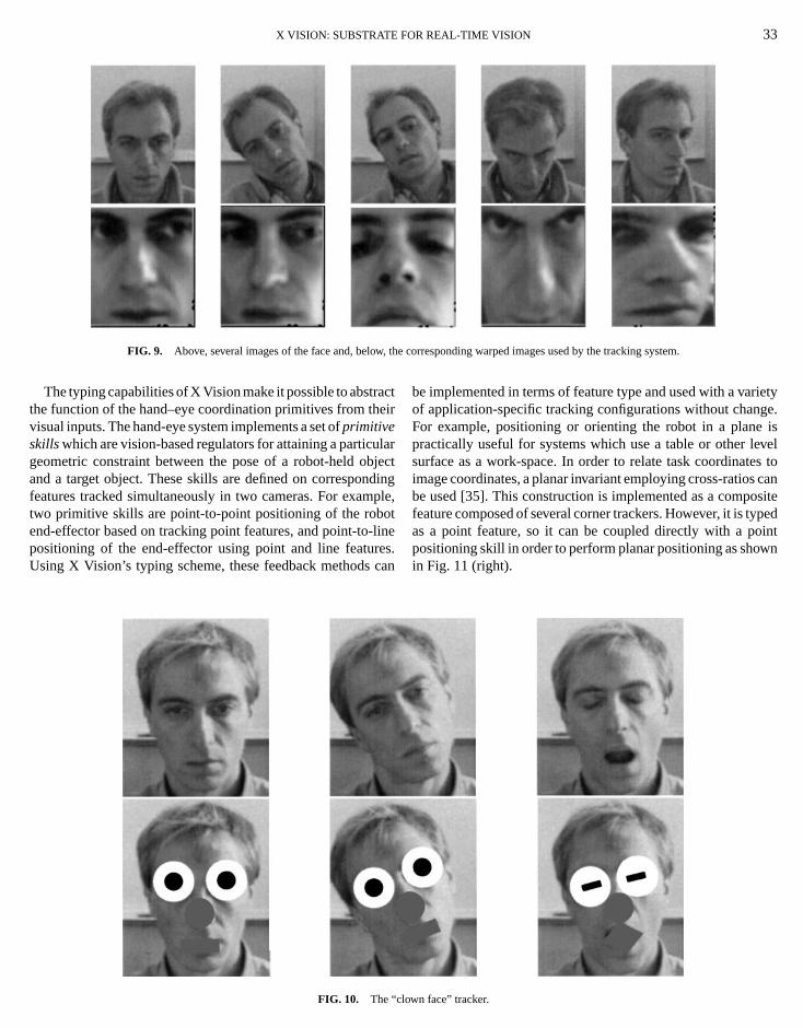
Region-based face trackingA frontal view of a human faceis sufficiently planar to be successfully tracked as a single SSDregion. Figure 9 shows several image pairs illustrating poses ofa face and the warped image resulting from tracking. Despitethe fact that the face is nonplanar, resulting, for example, in astretching of the nose as the face is turned, the tracking is quiteeffective. However, tracking a face as a single region requiresaffine warping over a relatively large region which is somewhatslow (about 40 ms per iteration). It can be confused if the faceundergoes distortions which cannot be easily captured by affinedeformation, and it is sensitive to lighting variations and shad-owing. Also, many areas of the face contain no strong gradients,thus contributing little to the state computation.

Figure 8 shows the structure of a more specialized trackingarrangement that uses SSD trackers at the regions of highestcontrast—the eyes and mouth. The result is a gain in perfor-mance as well as the ability to recognize isolated changes inthe underlying features. For each of the eyes and the mouth,

a MultiSSD composite tracker performs an SSD computa-tion for multiple reference images. The state of theMultiSSDtracker is computed to be the state of the tracker with the bestmatch value and the numeric identity of this tracker. The con-straint function copies this state back down to the componentSSD trackers, forcing “losing” SSD trackers to follow the “win-ner.” In effect, theMultiSSD feature is a tracker with ann-aryswitch.

From MultiSSD we derive anEye tracker which modi-fies the display function ofMultiSSD to show an open orclosed eye based on the state of the binary switch. We also de-rive Mouth which similarly displays an open or closed mouth.Two Eye ’s compose theEyes tracker. The state computationfunction of Eyes computes the orientation of the line joiningthe eyes, which is propagated to the lower-levelEye trackers,obviating the need to compute orientation from image-level in-formation. Thus, the low-levelEye trackers only solve for trans-lation, much as the disk tracker described above. Since the mouthcan move independently,Mouth computes both translation andorientation directly from the image. Finally, theFace trackercomprisesEyes andMouth . It imposes no constraints on them,but it does interpolate the position of the nose based on theEyesandMouth .

The tracker is initialized by indicating the positions of theeyes and mouth and memorizing their appearance when they areclosed and open. When run, the net effect is a graphical displayof a “clown face” that mimics the antics of the underlying humanface—the mouth and eyes follow those of the operator and openand close as the operator’s do as shown in Fig. 10. This systemrequires less than 10 ms per iteration without graphics.

3.2. An Embedded Application

As an illustration of the use of X Vision embedded withina larger system, we describe some results of using X Visionwithin a hand–eye coordination system [20, 22, 53]. The systemrelies on image-level feedback from two cameras to control therelative pose between an object held in a robot end-effector anda static object in the environment.

FIG. 8. The tracking network used for face tracking.

X VISION: SUBSTRATE FOR REAL-TIME VISION 33

FIG. 9. Above, several images of the face and, below, the corresponding warped images used by the tracking system.

The typing capabilities of X Vision make it possible to abstractthe function of the hand–eye coordination primitives from theirvisual inputs. The hand-eye system implements a set ofprimitiveskillswhich are vision-based regulators for attaining a particulargeometric constraint between the pose of a robot-held objectand a target object. These skills are defined on correspondingfeatures tracked simultaneously in two cameras. For example,two primitive skills are point-to-point positioning of the robotend-effector based on tracking point features, and point-to-linepositioning of the end-effector using point and line features.Using X Vision’s typing scheme, these feedback methods can

FIG. 10. The “clown face” tracker.

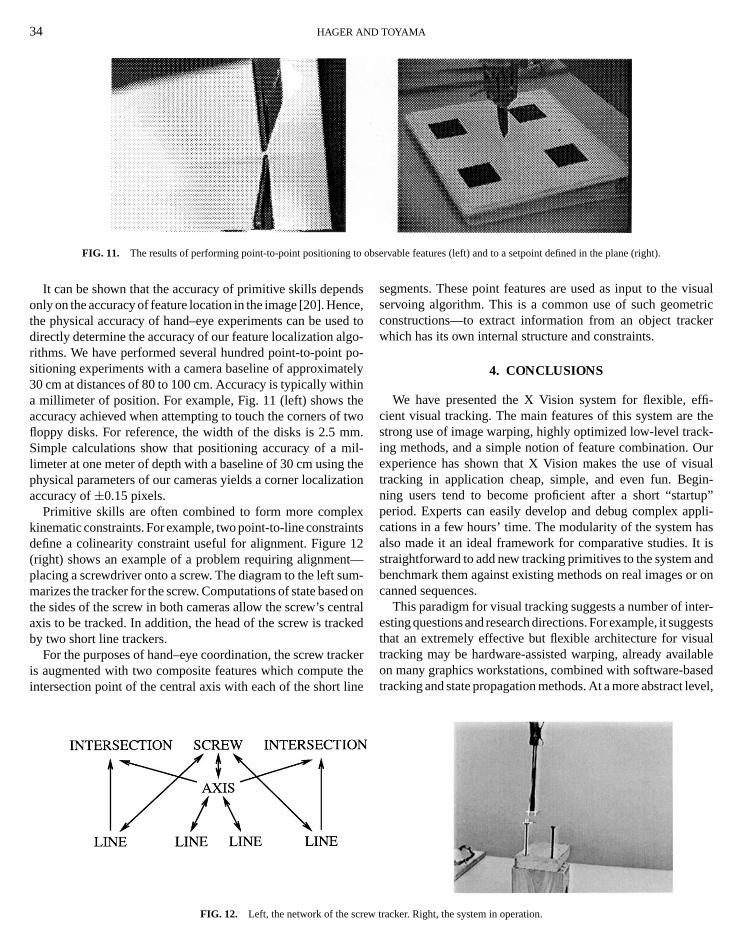
be implemented in terms of feature type and used with a varietyof application-specific tracking configurations without change.For example, positioning or orienting the robot in a plane ispractically useful for systems which use a table or other levelsurface as a work-space. In order to relate task coordinates toimage coordinates, a planar invariant employing cross-ratios canbe used [35]. This construction is implemented as a compositefeature composed of several corner trackers. However, it is typedas a point feature, so it can be coupled directly with a pointpositioning skill in order to perform planar positioning as shownin Fig. 11 (right).

34 HAGER AND TOYAMA

FIG. 11. The results of performing point-to-point positioning to observable features (left) and to a setpoint defined in the plane (right).

It can be shown that the accuracy of primitive skills dependsonly on the accuracy of feature location in the image [20]. Hence,the physical accuracy of hand–eye experiments can be used todirectly determine the accuracy of our feature localization algo-rithms. We have performed several hundred point-to-point po-sitioning experiments with a camera baseline of approximately30 cm at distances of 80 to 100 cm. Accuracy is typically withina millimeter of position. For example, Fig. 11 (left) shows theaccuracy achieved when attempting to touch the corners of twofloppy disks. For reference, the width of the disks is 2.5 mm.Simple calculations show that positioning accuracy of a mil-limeter at one meter of depth with a baseline of 30 cm using thephysical parameters of our cameras yields a corner localizationaccuracy of±0.15 pixels.

Primitive skills are often combined to form more complexkinematic constraints. For example, two point-to-line constraintsdefine a colinearity constraint useful for alignment. Figure 12(right) shows an example of a problem requiring alignment—placing a screwdriver onto a screw. The diagram to the left sum-marizes the tracker for the screw. Computations of state based onthe sides of the screw in both cameras allow the screw’s centralaxis to be tracked. In addition, the head of the screw is trackedby two short line trackers.

For the purposes of hand–eye coordination, the screw trackeris augmented with two composite features which compute theintersection point of the central axis with each of the short line

FIG. 12. Left, the network of the screw tracker. Right, the system in operation.

segments. These point features are used as input to the visualservoing algorithm. This is a common use of such geometricconstructions—to extract information from an object trackerwhich has its own internal structure and constraints.

4. CONCLUSIONS

We have presented the X Vision system for flexible, effi-cient visual tracking. The main features of this system are thestrong use of image warping, highly optimized low-level track-ing methods, and a simple notion of feature combination. Ourexperience has shown that X Vision makes the use of visualtracking in application cheap, simple, and even fun. Begin-ning users tend to become proficient after a short “startup”period. Experts can easily develop and debug complex appli-cations in a few hours’ time. The modularity of the system hasalso made it an ideal framework for comparative studies. It isstraightforward to add new tracking primitives to the system andbenchmark them against existing methods on real images or oncanned sequences.

This paradigm for visual tracking suggests a number of inter-esting questions and research directions. For example, it suggeststhat an extremely effective but flexible architecture for visualtracking may be hardware-assisted warping, already availableon many graphics workstations, combined with software-basedtracking and state propagation methods. At a more abstract level,

X VISION: SUBSTRATE FOR REAL-TIME VISION 35

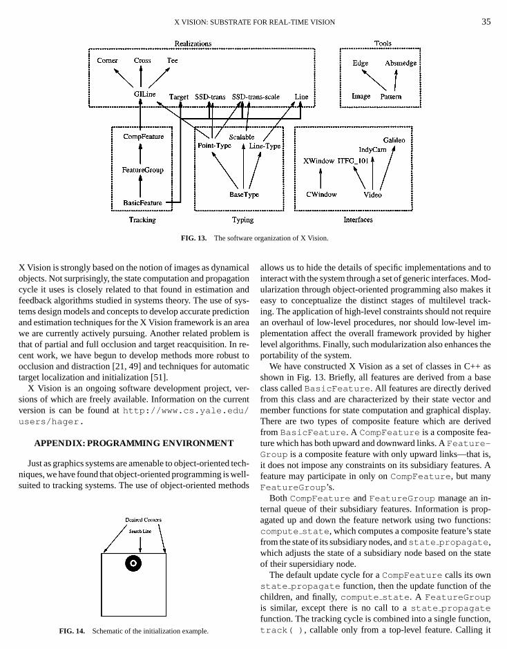
FIG. 13. The software organization of X Vision.

X Vision is strongly based on the notion of images as dynamicalobjects. Not surprisingly, the state computation and propagationcycle it uses is closely related to that found in estimation andfeedback algorithms studied in systems theory. The use of sys-tems design models and concepts to develop accurate predictionand estimation techniques for the X Vision framework is an areawe are currently actively pursuing. Another related problem isthat of partial and full occlusion and target reacquisition. In re-cent work, we have begun to develop methods more robust toocclusion and distraction [21, 49] and techniques for automatictarget localization and initialization [51].

X Vision is an ongoing software development project, ver-sions of which are freely available. Information on the currentversion is can be found athttp://www.cs.yale.edu/users/hager.

APPENDIX: PROGRAMMING ENVIRONMENT

Just as graphics systems are amenable to object-oriented tech-niques, we have found that object-oriented programming is well-suited to tracking systems. The use of object-oriented methods

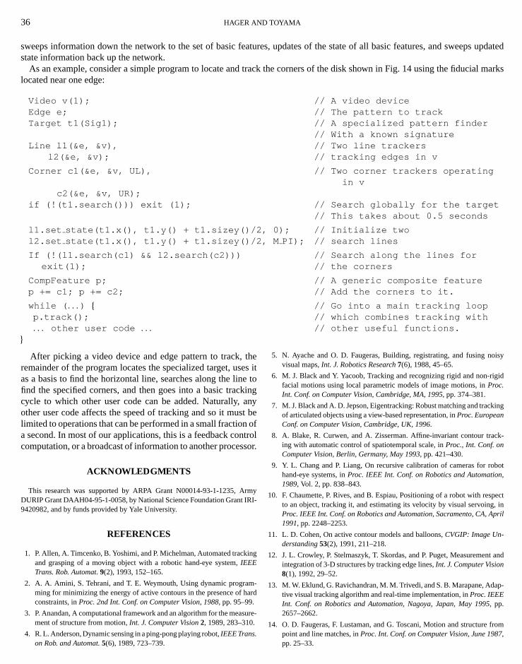
FIG. 14. Schematic of the initialization example.

allows us to hide the details of specific implementations and tointeract with the system through a set of generic interfaces. Mod-ularization through object-oriented programming also makes iteasy to conceptualize the distinct stages of multilevel track-ing. The application of high-level constraints should not requirean overhaul of low-level procedures, nor should low-level im-plementation affect the overall framework provided by higherlevel algorithms. Finally, such modularization also enhances theportability of the system.

We have constructed X Vision as a set of classes in C++ asshown in Fig. 13. Briefly, all features are derived from a baseclass calledBasicFeature . All features are directly derivedfrom this class and are characterized by their state vector andmember functions for state computation and graphical display.There are two types of composite feature which are derivedfrom BasicFeature . A CompFeature is a composite fea-ture which has both upward and downward links. AFeature-Group is a composite feature with only upward links—that is,it does not impose any constraints on its subsidiary features. Afeature may participate in only onCompFeature , but manyFeatureGroup ’s.

Both CompFeature andFeatureGroup manage an in-ternal queue of their subsidiary features. Information is prop-agated up and down the feature network using two functions:compute state , which computes a composite feature’s statefrom the state of its subsidiary nodes, andstate propagate ,which adjusts the state of a subsidiary node based on the stateof their supersidiary node.

The default update cycle for aCompFeature calls its ownstate propagate function, then the update function of thechildren, and finally,compute state . A FeatureGroupis similar, except there is no call to astate propagatefunction. The tracking cycle is combined into a single function,track( ) , callable only from a top-level feature. Calling it

36 HAGER AND TOYAMA

sweeps information down the network to the set of basic features, updates of the state of all basic features, and sweeps updatedstate information back up the network.

As an example, consider a simple program to locate and track the corners of the disk shown in Fig. 14 using the fiducial markslocated near one edge:

Video v(1); // A video deviceEdge e; // The pattern to trackTarget t1(Sig1); // A specialized pattern finder

// With a known signatureLine l1(&e, &v), // Two line trackers

l2(&e, &v); // tracking edges in v

Corner c1(&e, &v, UL), // Two corner trackers operatingin v

c2(&e, &v, UR);if (!(t1.search())) exit (1); // Search globally for the target

// This takes about 0.5 seconds

l1.set state(t1.x(), t1.y() + t1.sizey()/2, 0); // Initialize twol2.set state(t1.x(), t1.y() + t1.sizey()/2, M PI); // search lines

If (!(l1.search(c1) && l2.search(c2))) // Search along the lines forexit(1); // the corners

CompFeature p; // A generic composite featurep += c1; p += c2; // Add the corners to it.

while ( . . . ) { // Go into a main tracking loopp.track(); // which combines tracking with. . . other user code . . . // other useful functions.

}After picking a video device and edge pattern to track, the

remainder of the program locates the specialized target, uses itas a basis to find the horizontal line, searches along the line tofind the specified corners, and then goes into a basic trackingcycle to which other user code can be added. Naturally, anyother user code affects the speed of tracking and so it must belimited to operations that can be performed in a small fraction ofa second. In most of our applications, this is a feedback controlcomputation, or a broadcast of information to another processor.

ACKNOWLEDGMENTS

This research was supported by ARPA Grant N00014-93-1-1235, ArmyDURIP Grant DAAH04-95-1-0058, by National Science Foundation Grant IRI-9420982, and by funds provided by Yale University.

REFERENCES

1. P. Allen, A. Timcenko, B. Yoshimi, and P. Michelman, Automated trackingand grasping of a moving object with a robotic hand-eye system,IEEETrans. Rob. Automat.9(2), 1993, 152–165.

2. A. A. Amini, S. Tehrani, and T. E. Weymouth, Using dynamic program-ming for minimizing the energy of active contours in the presence of hardconstraints, inProc. 2nd Int. Conf. on Computer Vision, 1988,pp. 95–99.

3. P. Anandan, A computational framework and an algorithm for the measure-ment of structure from motion,Int. J. Computer Vision2, 1989, 283–310.

4. R. L. Anderson, Dynamic sensing in a ping-pong playing robot,IEEE Trans.on Rob. and Automat.5(6), 1989, 723–739.

5. N. Ayache and O. D. Faugeras, Building, registrating, and fusing noisyvisual maps,Int. J. Robotics Research7(6), 1988, 45–65.

6. M. J. Black and Y. Yacoob, Tracking and recognizing rigid and non-rigidfacial motions using local parametric models of image motions, inProc.Int. Conf. on Computer Vision, Cambridge, MA, 1995, pp. 374–381.

7. M. J. Black and A. D. Jepson, Eigentracking: Robust matching and trackingof articulated objects using a view-based representation, inProc. EuropeanConf. on Computer Vision, Cambridge, UK, 1996.

8. A. Blake, R. Curwen, and A. Zisserman. Affine-invariant contour track-ing with automatic control of spatiotemporal scale, inProc., Int. Conf. onComputer Vision, Berlin, Germany, May 1993, pp. 421–430.

9. Y. L. Chang and P. Liang, On recursive calibration of cameras for robothand-eye systems, inProc. IEEE Int. Conf. on Robotics and Automation,1989, Vol. 2, pp. 838–843.

10. F. Chaumette, P. Rives, and B. Espiau, Positioning of a robot with respectto an object, tracking it, and estimating its velocity by visual servoing, inProc. IEEE Int. Conf. on Robotics and Automation, Sacramento, CA, April1991, pp. 2248–2253.

11. L. D. Cohen, On active contour models and balloons,CVGIP: Image Un-derstanding53(2), 1991, 211–218.

12. J. L. Crowley, P. Stelmaszyk, T. Skordas, and P. Puget, Measurement andintegration of 3-D structures by tracking edge lines,Int. J. Computer Vision8(1), 1992, 29–52.

13. M. W. Eklund, G. Ravichandran, M. M. Trivedi, and S. B. Marapane, Adap-tive visual tracking algorithm and real-time implementation, inProc. IEEEInt. Conf. on Robotics and Automation, Nagoya, Japan, May 1995, pp.2657–2662.

14. O. D. Faugeras, F. Lustaman, and G. Toscani, Motion and structure frompoint and line matches, inProc. Int. Conf. on Computer Vision, June 1987,pp. 25–33.

X VISION: SUBSTRATE FOR REAL-TIME VISION 37

15. J. D. Foley, A. van Dam, S. K. Feiner, and J. F. Hughes,Computer Graphics,Addison-Wesley, Reading, MA, 1993.

16. W. T. Freeman and E. H. Adelson, Steerable filters for early vision, im-age analysis, and wavelet decomposition, inProc., Int. Conf. on ComputerVision, Osaka, Japan, 1990.

17. D. B. Gennery, Visual tracking of known three-dimensional objects,Int. J.Computer Vision, 7(3), 1992, 243–270.

18. G. D. Hager, Calibration-free visual control using projective invariance, inInt. Conf. on Computer Vision, Cambridge, MA, 1995, pp. 1009–1015.

19. G. D. Hager, Real-time feature tracking and projective invariance as a basisfor hand–eye coordination, inComputer Vision and Pattern Recognition,pp. 533–539, IEEE Computer Soc., Los Alamitos, CA, 1994.

20. G. D. Hager, A modular system for robust hand–eye coordination usingfeedback from stereo vision,IEEE Trans. Robotics Automation13(4), 1997,582–595.

21. G. D. Hager and P. N. Belhumeur, Real-time tracking of image regionswith changes in geometry and illumination, inComputer Vision and PatternRecognition, pp. 403–410, IEEE Computer Soc., Los Alamitos, CA, 1996.

22. G. D. Hager, W.-C. Chang, and A. S. Morse, Robot hand–eye coordinationbased on stereo vision,IEEE Control Systems Mag. 15(1), 1995, 30–39.

23. G. D. Hager, G. Grunwald, and K. Toyama, Feature-based visual servo-ing and its application to telerobotics, inIntelligent Robots and Systems(V. Graefe, Ed.), Elsevier, Amsterdam, 1995.

24. R. M. Haralick and L. G. Shapiro,Computer and Robot Vision: Vol. II,Addison-Wesley, Reading, MA, 1993.

25. T. Heikkila, Matsushita, and Sato, Planning of visual feedback with robot-sensor co-operation, inProc. IEEE Int. Workshop on Intelligent Robots andSystems, Tokyo, 1988.

26. E. Huber and D. Kortenkamp, Using stereo vision to pursue moving agentswith a mobile robot, inProc. IEEE Int. Conf. on Robotics and Automation,Nagoya, Japan, May 1995, pp. 2340–2346.

27. I. Inoue, Hand eye coordination in rope handling, in1st Int. Symp. OnRobotics Research, Bretten Woods, 1983.

28. A. Izaguirre, P. Pu, and J. Summers, A new development in camera calibra-tion: Calibrating a pair of mobile cameras,Int. J. Robot. Res.6(3), 1987,104–116.

29. H. Kass, A. Witkin, and D. Terzopoulos, Snakes: Active contour models,Int. J. Computer Vision1, 1987, 321–331.

30. Y. Liu and T. S. Huang, A linear algorithm for motion estimation usingstraight line correspondences, inInt. Conf. on Pattern Recognition, 1988,pp. 213–219.

31. D. G. Lowe, Robust model-based motion tracking through the integrationof search and estimation,Int. J. Computer Vision8(2), 1992, 113–122.

32. C.-P. Lu,Online Pose Estimation and Model Matching, Ph.D. thesis, YaleUniversity, 1995.

33. B. D. Lucas and T. Kanade, An iterative image registration technique withan application to stereo vision, 1981, pp. 674–679.

34. A. D. Morgan, E. L. Dagless, D. J. Milford, and B. T. Thomas, Road edgetracking for robot road following: A real-time implementation,Image VisionComput. 8(3), 1990, 233–240.

35. J. Mundy and A. Zisserman,Geometric Invariance in Computer Vision,MIT Press, Cambridge, MA, 1992.

36. H. K. Nishihara, Teleos AVP, inCVPR Demo Program, San Francisco,1996.

37. N. Papanikolopoulos, P. Khosla, and T. Kanade, Visual tracking of a movingtarget by a camera mounted on a robot: A combination of control and vision,in Proc. IEEE Int. Conf. on Robot. Automat.9(1), 1993.

38. D. Reynard, A. Wildenberg, A. Blake, and J. Marchant, Learning dynamicsof complex motions from image sequences,I , 1996, 357–368.

39. A. A. Rizzi and D. E. Koditschek, An active visual estimator for dexterousmanipulation at theWorkshop on Visual Servoing, 1994.

40. J. Shi and C. Tomasi, Good features to track, inComputer Vision and PatternRecognition, pp. 593–600, IEEE Computer Soc. 1994.

41. D. Sinclair, A. Blake, S. Smith, and C. Rothwell, Planar region detectionand motion recovery,Image and Vision Computing11(4), 1993, 229–234.

42. M. E. Spetsakis, A linear algorithm for point and line-based structure frommotion.CVGIP: Image Understanding56(2), 1992, 230–241.

43. M. E. Spetsakis and J. Aloimonos, Structure from motion using line corre-spondences,Int. J. Computer Vision4, 1990, 171–183.

44. T. N. Tan, K. D. Baker, and G. D. Sullivan, 3D structure and motion estima-tion from 2D image sequences,Image and Vision Computing11(4), 1993,203–210.

45. Camillo J. Taylor and D. J. Kriegman, Structure and motion from linesegments in multiple images, inProc. IEEE Int. Conf. on Robotics andAutomation, 1992,pp. 1615–1620.

46. D. Terzopoulos and R. Szeliski, Tracking with Kalman snakes, inActiveVision(A. Blake and A. Yuille, Eds.), MIT Press, Cambridge, MA, 1992.

47. C. Tomasi and T. Kanade, Shape and motion from image streams: A fac-torization method, full report on the orthographic case, CMU-CS 92-104,CMU, 1992.

48. C. Tomasi and T. Kanade, Shape and motion without depth, inProc. ImageUnderstanding Workshop, September 1990, pp. 258–271.

49. K. Toyama and G. D. Hager, Keeping your eye on the ball: Tracking occlud-ing contours of unfamiliar objects without distraction, inProc. Int. Conf.on Intel. Robotics and Sys., Pittsburgh, PA, August 1995, pp. 354–359.

50. K. Toyama and G. D. Hager, Tracker fusion for robustness in visual featuretracking, inSPIE Int. Sym. Intel. Sys. and Adv. Manufacturing, Philadelphia,PA, October 1995, Vol. 2589.

51. K. Toyama and G. D. Hager, Incremental focus of attention for robust visualtracking, inComputer Vision and Pattern Recognition,pp. 189–195, IEEEComput. Soc., Los Alamitos, CA, 1996.

52. K. Toyama and G. D. Hager, Vision-based 3D “Surfball” input device, 1996,provisional patent application field through Yale Office of Cooperative Re-search, OCR 770.

53. K. Toyama, J. Wang, and G. D. Hager, SERVOMATIC: A modular sys-tem for robust positioning using stereo visual servoing, inProc. Int. Conf.Robotics and Automation, 1996, pp. 2636–2643.

54. D. J. Williams and M. Shah, A fast algorithm for active contours and cur-vature estimation.CVGIP: Image Understanding55(1), 1992, 14–26.

55. Y. Yagi, K. Sato, and M. Yachida, Evaluating effectivity of map generationby tracking vertical edges in omnidirectional image sequence, inProc.IEEE Int. Conf. on Robotics and Automation, Nagoya, Japan, May 1995,pp. 2334–2339.

56. B. H. Yoshimi and P. K. Allen, Active, uncalibrated visual servoing, inProc.IEEE Int. Conf. on Robotics and Automation, San Diego, CA, May 1994,Vol. 4, pp. 156–161.

57. Z. Zhang and O. Faugeras, Determining motion from 3D line segmentmatches: A comparative study,Image Vision Comput. 9(1), 1991, 10–19.