X uniformly probability distribution probability density … · 2013-10-06 · CH 5 Normal...
43
CH 5 Normal Probability Distributions Properties of the Normal Distribution Example A friend that is always late. Let X represent the amount of minutes that pass from the moment you are suppose to meet your friend until the moment your friend showed up. Suppose your friend is just as likely to arrive at any time between x = 0 and x = 30 minutes late. That is, the random variable X can take any value in the interval [0, 30] . In this case we will say that the random variable X follows a uniformly probability distribution. What is the probability that your friend will arrive exactly 5 minutes late? What is the probability that your friend will arrive between 5 and 10 minutes late? This is what we call probability density functions
Transcript of X uniformly probability distribution probability density … · 2013-10-06 · CH 5 Normal...
CH 5 Normal Probability Distributions
Properties of the Normal Distribution
Example
A friend that is always late. Let X represent the amount of minutes thatpass from the moment you are suppose to meet your friend until themoment your friend showed up.
Suppose your friend is just as likely to arrive at any time between x = 0and x = 30 minutes late.
That is, the random variable X can take any value in the interval [0, 30] .
In this case we will say that the random variable X follows a uniformlyprobability distribution.
What is the probability that your friend will arrive exactly 5 minutes late?
What is the probability that your friend will arrive between 5 and 10minutes late?
This is what we call probability density functions
CH 5 Normal Probability Distributions
Properties of the Normal Distribution
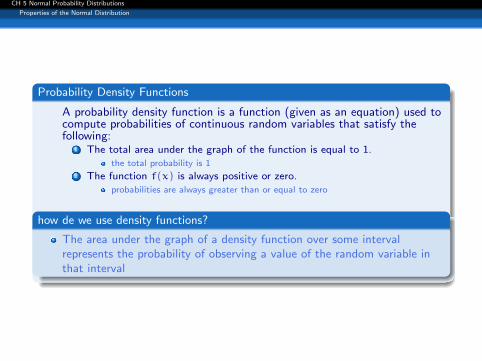
Probability Density Functions
A probability density function is a function (given as an equation) used tocompute probabilities of continuous random variables that satisfy thefollowing:
1 The total area under the graph of the function is equal to 1.the total probability is 1
2 The function f(x) is always positive or zero.probabilities are always greater than or equal to zero
how de we use density functions?
The area under the graph of a density function over some intervalrepresents the probability of observing a value of the random variable inthat interval
CH 5 Normal Probability Distributions
Properties of the Normal Distribution
mode, median and mode in a density function
For any distributionthe mode represents the high pointThe median is the point where 50% of the area of the distribution is on theleft.
CH 5 Normal Probability Distributions
Properties of the Normal Distribution
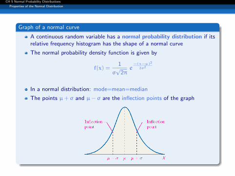
Graph of a normal curve
A continuous random variable has a normal probability distribution if itsrelative frequency histogram has the shape of a normal curve
The normal probability density function is given by
f(x) =1
σ√
2πe
−(x−µ)2
2σ2
In a normal distribution: mode=mean=median
The points µ+ σ and µ− σ are the inflection points of the graph
CH 5 Normal Probability Distributions
Properties of the Normal Distribution
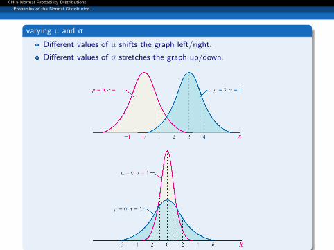
varying µ and σ
Different values of µ shifts the graph left/right.
Different values of σ stretches the graph up/down.
CH 5 Normal Probability Distributions
Properties of the Normal Distribution
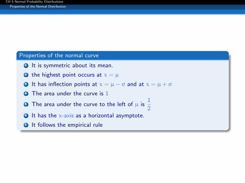
Properties of the normal curve
1 It is symmetric about its mean.
2 the highest point occurs at x = µ
3 It has inflection points at x = µ− σ and at x = µ+ σ
4 The area under the curve is 1
5 The area under the curve to the left of µ is1
26 It has the x-axis as a horizontal asymptote.
7 It follows the empirical rule
CH 5 Normal Probability Distributions
Properties of the Normal Distribution
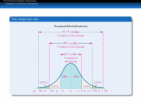
The empirical rule
CH 5 Normal Probability Distributions
Properties of the Normal Distribution
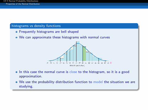
histograms vs density functions
Frequently histograms are bell shaped
We can approximate these histograms with normal curves
In this case the normal curve is close to the histogram, so it is a goodapproximation.
We use the probability distribution function to model the situation we arestudying.
CH 5 Normal Probability Distributions
Properties of the Normal Distribution
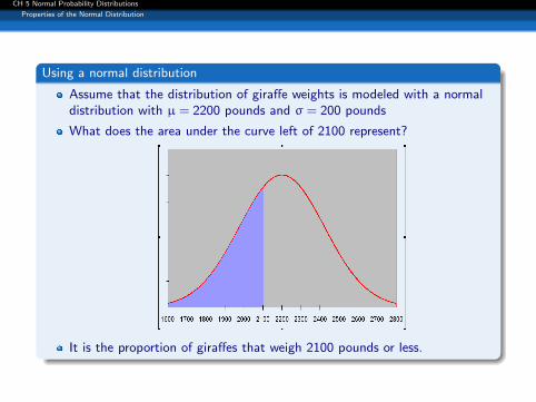
Using a normal distribution
Assume that the distribution of giraffe weights is modeled with a normaldistribution with µ = 2200 pounds and σ = 200 pounds
What does the area under the curve left of 2100 represent?
It is the proportion of giraffes that weigh 2100 pounds or less.
CH 5 Normal Probability Distributions
Properties of the Normal Distribution
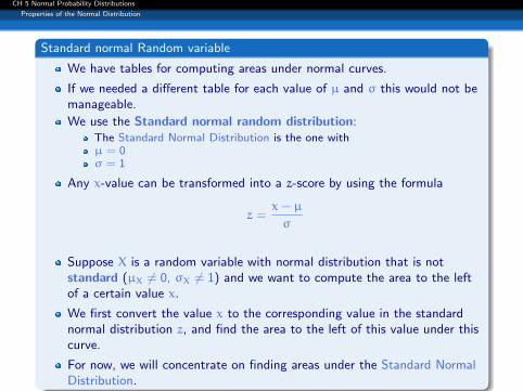
Standard normal Random variable
We have tables for computing areas under normal curves.
If we needed a different table for each value of µ and σ this would not bemanageable.
We use the Standard normal random distribution:The Standard Normal Distribution is the one withµ = 0σ = 1
Any x-value can be transformed into a z-score by using the formula
z =x− µ
σ
Suppose X is a random variable with normal distribution that is notstandard (µX 6= 0, σX 6= 1) and we want to compute the area to the leftof a certain value x.
We first convert the value x to the corresponding value in the standardnormal distribution z, and find the area to the left of this value under thiscurve.
For now, we will concentrate on finding areas under the Standard NormalDistribution.
CH 5 Normal Probability Distributions
Properties of the Normal Distribution
Calculating the area to the left of z0
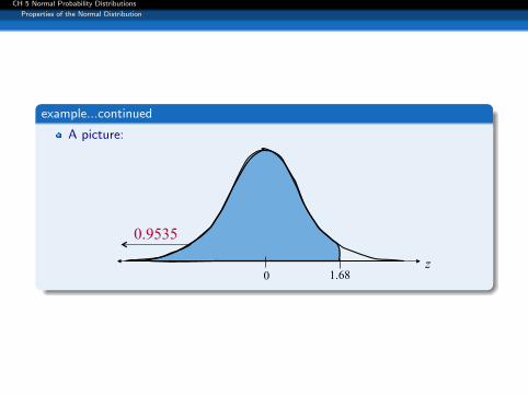
Find the area under the standard normal curve that lies to the left ofz = 1.68
CH 5 Normal Probability Distributions
Properties of the Normal Distribution
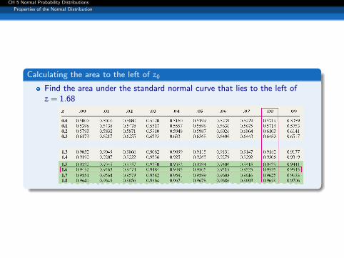
Calculating the area to the left of z0
Find the area under the standard normal curve that lies to the left ofz = 1.68
CH 5 Normal Probability Distributions
Properties of the Normal Distribution
example...continued
A picture:
0.9535
1.68 0 z
CH 5 Normal Probability Distributions
Properties of the Normal Distribution
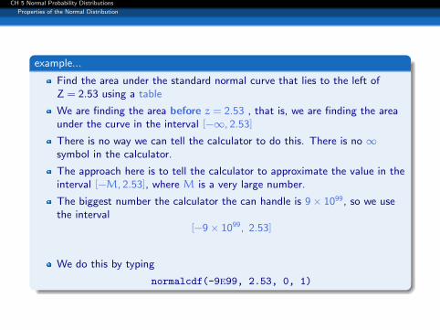
example...
Find the area under the standard normal curve that lies to the left ofZ = 2.53 using a table
We are finding the area before z = 2.53 , that is, we are finding the areaunder the curve in the interval [−∞, 2.53]
There is no way we can tell the calculator to do this. There is no ∞symbol in the calculator.
The approach here is to tell the calculator to approximate the value in theinterval [−M, 2.53], where M is a very large number.
The biggest number the calculator the can handle is 9× 1099, so we usethe interval
[−9× 1099, 2.53]
We do this by typing
normalcdf(-9e99, 2.53, 0, 1)
CH 5 Normal Probability Distributions
Properties of the Normal Distribution
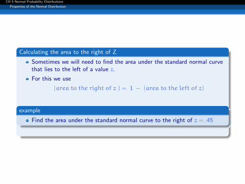
Calculating the area to the right of Z
Sometimes we will need to find the area under the standard normal curvethat lies to the left of a value z.
For this we use
(area to the right of z ) = 1 − (area to the left of z)
example
Find the area under the standard normal curve to the right of z = .45
CH 5 Normal Probability Distributions
Properties of the Normal Distribution
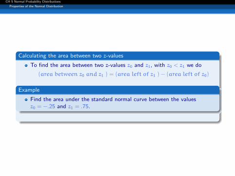
Calculating the area between two z-values
To find the area between two z-values z0 and z1, with z0 < z1 we do
(area between z0 and z1 ) = (area left of z1 ) − (area left of z0)
Example
Find the area under the standard normal curve between the valuesz0 = −.25 and z1 = .75.
CH 5 Normal Probability Distributions
Properties of the Normal Distribution
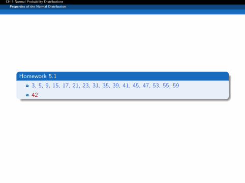
Homework 5.1
3, 5, 9, 15, 17, 21, 23, 31, 35, 39, 41, 45, 47, 53, 55, 59
42

CH 5 Normal Probability Distributions
5.2 Normal Distributions: Finding Probabilities
If a random variable x is normally distributed, you can find the probabilitythat x will fall in a given interval by calculating the area under the normalcurve for the given interval
To find the area under any normal curve we can first convert the upperand lower bound of the interval into z-scores , then use the standardnormal distribution to find the area.
Normal Distribution
600 µ =500
P(x < 600)
µ = 500 σ = 100
x
Standard Normal Distribution
1 µ = 0
µ = 0 σ = 1
z
P(z < 1)
P(x < 500) = P(z < 1) Same Area
CH 5 Normal Probability Distributions
5.2 Normal Distributions: Finding Probabilities
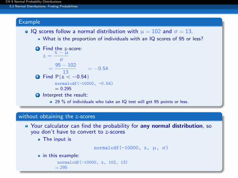
Example
IQ scores follow a normal distribution with µ = 102 and σ = 13.What is the proportion of individuals with an IQ scores of 95 or less?
1 Find the z-score:
z =x−µ
σ
=95 − 102
13= −0.54
2 Find P(z < −0.54)normalcdf(-10000, -0.54)= 0.295
3 Interpret the result:29 % of individuals who take an IQ test will get 95 points or less.
without obtaining the z-scores
Your calculator can find the probability for any normal distribution, soyou don’t have to convert to z-scores
The input is
normalcdf(-10000, x, µ, σ)
in this example:normalcdf(-10000, x, 102, 13)
=.295
CH 5 Normal Probability Distributions
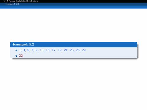
Homework 5.2
Homework 5.2
1, 3, 5, 7, 9, 13, 15, 17, 19, 21, 23, 25, 29
22
CH 5 Normal Probability Distributions
5.3 Finding values
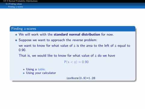
Finding z-scores
Finding z-scores
We will work with the standard normal distribution for now.
Suppose we want to approach the reverse problem:
we want to know for what value of z is the area to the left of z equal to0.90.
That is, we would like to know for what value of z do we have
P(x < z) = 0.90
Using a table.Using your calculator
invNorm(0.9)=1.28
CH 5 Normal Probability Distributions
5.3 Finding values
Finding z-scores
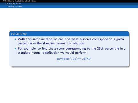
percentiles
With this same method we can find what z-scores correspond to a givenpercentile in the standard normal distribution.
For example, to find the z-score corresponding to the 25th percentile in astandard normal distribution we would perform:
invNorm(.25)=-.6749
CH 5 Normal Probability Distributions
5.3 Finding values
Finding z-scores
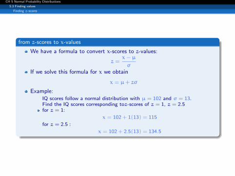
from z-scores to x-values
We have a formula to convert x-scores to z-values:
z =x− µ
σIf we solve this formula for x we obtain
x = µ+ zσ
Example:IQ scores follow a normal distribution with µ = 102 and σ = 13.Find the IQ scores corresponding toz-scores of z = 1, z = 2.5for z = 1:
x = 102 + 1(13) = 115
for z = 2.5 :
x = 102 + 2.5(13) = 134.5
CH 5 Normal Probability Distributions
5.3 Finding values
Finding z-scores
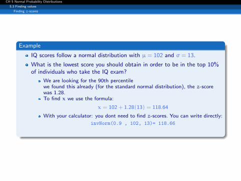
Example
IQ scores follow a normal distribution with µ = 102 and σ = 13.
What is the lowest score you should obtain in order to be in the top 10%of individuals who take the IQ exam?
We are looking for the 90th percentilewe found this already (for the standard normal distribution), the z-scorewas 1.28.To find x we use the formula:
x = 102 + 1.28(13) = 118.64
With your calculator: you dont need to find z-scores. You can write directly:
invNorm(0.9 , 102, 13)= 118.66
CH 5 Normal Probability Distributions
5.3 Finding values
Finding z-scores
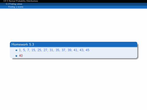
Homework 5.3
1, 5, 7, 15, 25, 27, 31, 35, 37, 39, 41, 43, 45
40
CH 5 Normal Probability Distributions
5.4 Distribution of the Sample mean
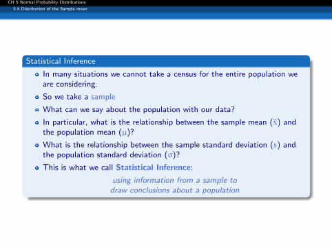
Statistical Inference
In many situations we cannot take a census for the entire population weare considering.
So we take a sample
What can we say about the population with our data?
In particular, what is the relationship between the sample mean (x̄) andthe population mean (µ)?
What is the relationship between the sample standard deviation (s) andthe population standard deviation (σ)?
This is what we call Statistical Inference:
using information from a sample todraw conclusions about a population
CH 5 Normal Probability Distributions
5.4 Distribution of the Sample mean
Estimate the Population Mean
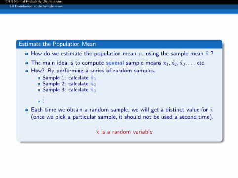
How do we estimate the population mean µ, using the sample mean x̄ ?
The main idea is to compute several sample means x̄1, x̄2, x̄3, . . . etc.
How? By performing a series of random samples.Sample 1: calculate x̄1
Sample 2: calculate x̄2
Sample 3: calculate x̄3
...
Each time we obtain a random sample, we will get a distinct value for x̄(once we pick a particular sample, it should not be used a second time).
x̄ is a random variable
CH 5 Normal Probability Distributions
5.4 Distribution of the Sample mean
x̄ as a random variable
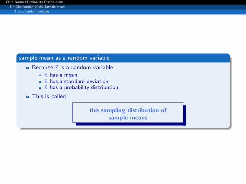
sample mean as a random variable
Because x̄ is a random variable:x̄ has a meanx̄ has a standard deviationx̄ has a probability distribution
This is called
the sampling distribution ofsample means
CH 5 Normal Probability Distributions
5.4 Distribution of the Sample mean
x̄ as a random variable
in-class example
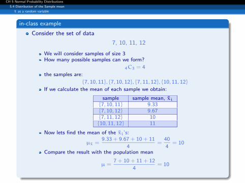
Consider the set of data
7, 10, 11, 12
We will consider samples of size 3How many possible samples can we form?
4C3 = 4
the samples are:
{7, 10, 11}, {7, 10, 12}, {7, 11, 12}, {10, 11, 12}
If we calculate the mean of each sample we obtain:
sample sample mean, x̄i{7, 10, 11} 9.33{7, 10, 12} 9.67{7, 11, 12} 10{10, 11, 12} 11
Now lets find the mean of the x̄i’s:
µx̄ =9.33 + 9.67 + 10 + 11
4=
40
4= 10
Compare the result with the population mean
µ =7 + 10 + 11 + 12
4= 10
CH 5 Normal Probability Distributions
5.4 Distribution of the Sample mean
x̄ as a random variable
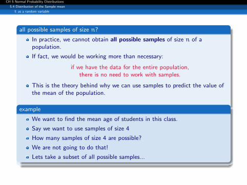
all possible samples of size n?
In practice, we cannot obtain all possible samples of size n of apopulation.
If fact, we would be working more than necessary:
if we have the data for the entire population,there is no need to work with samples.
This is the theory behind why we can use samples to predict the value ofthe mean of the population.
example
We want to find the mean age of students in this class.
Say we want to use samples of size 4
How many samples of size 4 are possible?
We are not going to do that!
Lets take a subset of all possible samples...
CH 5 Normal Probability Distributions
5.4 Distribution of the Sample mean
x̄ as a random variable
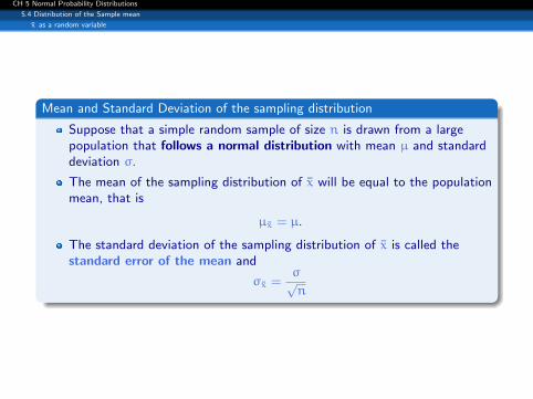
Mean and Standard Deviation of the sampling distribution
Suppose that a simple random sample of size n is drawn from a largepopulation that follows a normal distribution with mean µ and standarddeviation σ.
The mean of the sampling distribution of x̄ will be equal to the populationmean, that is
µx̄ = µ.
The standard deviation of the sampling distribution of x̄ is called thestandard error of the mean and
σx̄ =σ√n
CH 5 Normal Probability Distributions
5.4 Distribution of the Sample mean
x̄ as a random variable
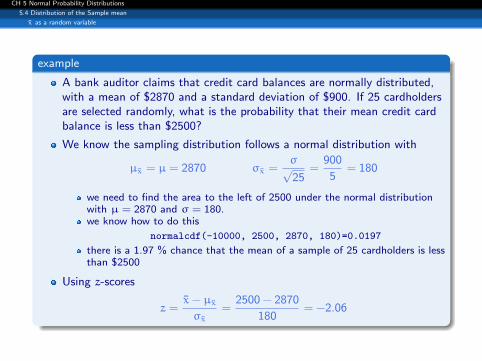
example
A bank auditor claims that credit card balances are normally distributed,with a mean of $2870 and a standard deviation of $900. If 25 cardholdersare selected randomly, what is the probability that their mean credit cardbalance is less than $2500?
We know the sampling distribution follows a normal distribution with
µx̄ = µ = 2870 σx̄ =σ√25
=900
5= 180
we need to find the area to the left of 2500 under the normal distributionwith µ = 2870 and σ = 180.we know how to do this
normalcdf(-10000, 2500, 2870, 180)=0.0197
there is a 1.97 % chance that the mean of a sample of 25 cardholders is lessthan $2500
Using z-scores
z =x̄− µx̄σx̄
=2500 − 2870
180= −2.06
CH 5 Normal Probability Distributions
5.4 Distribution of the Sample mean
The Central Limit Theorem
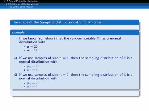
The shape of the Sampling distribution of x̄ for X normal
example
If we know (somehow) that the random variable X has a normaldistribution with
µ = 20σ = 12
1 If we use samples of size n = 4, then the sampling distribution of x̄ is anormal distribution with
µx̄ = 20σx̄ = 6
2 If we use samples of size n = 9, then the sampling distribution of x̄ is anormal distribution with
µx̄ = 20σx̄ = 4
CH 5 Normal Probability Distributions
5.4 Distribution of the Sample mean
The Central Limit Theorem
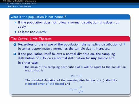
what if the population is not normal?
If the population does not follow a normal distribution this does notapply...
at least not exactly
The Central Limit Theorem
1 Regardless of the shape of the population, the sampling distribution of x̄becomes approximately normal as the sample size n increases.
2 If the population itself follows a normal distribution, the samplingdistribution of x̄ follows a normal distribution for any sample size.
In either case,the mean of the sampling distribution of x̄ will be equal to the populationmean, that is
µx̄ = µ.
The standard deviation of the sampling distribution of x̄ (called thestandard error of the mean) and
σx̄ =σ√n
CH 5 Normal Probability Distributions
5.4 Distribution of the Sample mean
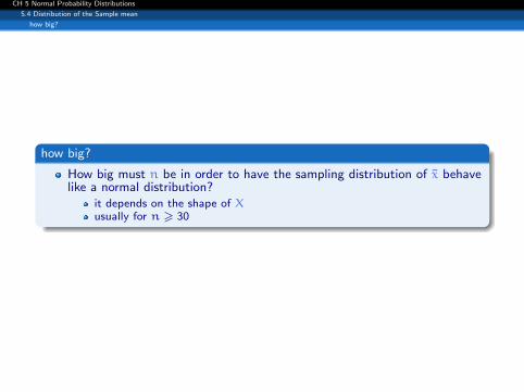
how big?
how big?
How big must n be in order to have the sampling distribution of x̄ behavelike a normal distribution?
it depends on the shape of Xusually for n > 30
CH 5 Normal Probability Distributions
5.4 Distribution of the Sample mean
how big?
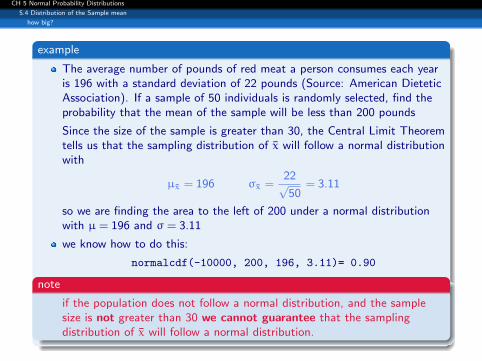
example
The average number of pounds of red meat a person consumes each yearis 196 with a standard deviation of 22 pounds (Source: American DieteticAssociation). If a sample of 50 individuals is randomly selected, find theprobability that the mean of the sample will be less than 200 pounds
Since the size of the sample is greater than 30, the Central Limit Theoremtells us that the sampling distribution of x̄ will follow a normal distributionwith
µx̄ = 196 σx̄ =22√50
= 3.11
so we are finding the area to the left of 200 under a normal distributionwith µ = 196 and σ = 3.11
we know how to do this:
normalcdf(-10000, 200, 196, 3.11)= 0.90
note
if the population does not follow a normal distribution, and the samplesize is not greater than 30 we cannot guarantee that the samplingdistribution of x̄ will follow a normal distribution.
CH 5 Normal Probability Distributions
5.4 Distribution of the Sample mean
how big?
Homework
9, 11, 13, 15, 19, 25, 27, 29, 31, 33
28
CH 5 Normal Probability Distributions
5.5 Normal Approximations to Binomial Distributions
Approximating a Binomial Distribution
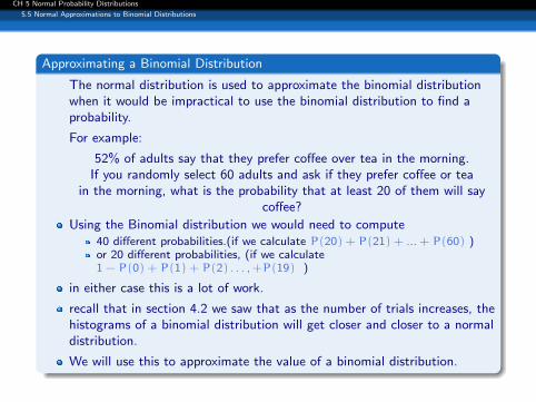
The normal distribution is used to approximate the binomial distributionwhen it would be impractical to use the binomial distribution to find aprobability.
For example:
52% of adults say that they prefer coffee over tea in the morning.If you randomly select 60 adults and ask if they prefer coffee or tea
in the morning, what is the probability that at least 20 of them will saycoffee?
Using the Binomial distribution we would need to compute40 different probabilities.(if we calculate P(20) + P(21) + ... + P(60) )or 20 different probabilities, (if we calculate1 − P(0) + P(1) + P(2) . . . ,+P(19) )
in either case this is a lot of work.
recall that in section 4.2 we saw that as the number of trials increases, thehistograms of a binomial distribution will get closer and closer to a normaldistribution.
We will use this to approximate the value of a binomial distribution.
CH 5 Normal Probability Distributions
5.5 Normal Approximations to Binomial Distributions
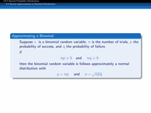
Approximating a Binomial
Suppose x is a binomial random variable, n is the number of trials, p theprobability of success, and q the probability of failure.
if
np > 5 and nq > 5
then the binomial random variable is follows approximately a normaldistribution with
µ = np and σ =√npq
CH 5 Normal Probability Distributions
5.5 Normal Approximations to Binomial Distributions
example
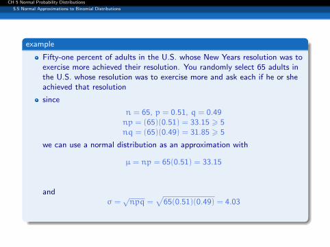
Fifty-one percent of adults in the U.S. whose New Years resolution was toexercise more achieved their resolution. You randomly select 65 adults inthe U.S. whose resolution was to exercise more and ask each if he or sheachieved that resolution
since
n = 65, p = 0.51, q = 0.49np = (65)(0.51) = 33.15 > 5nq = (65)(0.49) = 31.85 > 5
we can use a normal distribution as an approximation with
µ = np = 65(0.51) = 33.15
andσ =√npq =
√65(0.51)(0.49) = 4.03
CH 5 Normal Probability Distributions
5.5 Normal Approximations to Binomial Distributions
correction for continuity
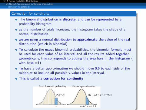
Correction for continuity
The binomial distribution is discrete, and can be represented by aprobability histogram
as the number of trials increases, the histogram takes the shape of anormal distribution.
we are using a normal distribution to approximate the value of the realdistribution (which is binomial)
To calculate the exact binomial probabilities, the binomial formula mustbe used for each value of an interval and all the results added together.geometrically, this corresponds to adding the area bars in the histogram (with base =1)
To have a better approximation we should move 0.5 to each side of themidpoint to include all possible x-values in the interval.
This is called a correction for continuity
Exact binomial probability
P(x = c)
c
Normal approximation
P(c – 0.5 < x < c + 0.5)
c c+ 0.5 c– 0.5
CH 5 Normal Probability Distributions
5.5 Normal Approximations to Binomial Distributions
correction for continuity
example... continued
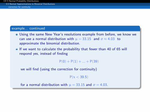
Using the same New Year’s resolutions example from before, we know wecan use a normal distribution with µ = 33.15 and σ ≈ 4.03 toapproximate the binomial distribution.
If we want to calculate the probability that fewer than 40 of 65 willrespond yes, instead of finding
P(0) + P(1) + ... + P(39)
we will find (using the correction for continuity)
P(x < 39.5)
for a normal distribution with µ = 33.15 and σ = 4.03.
CH 5 Normal Probability Distributions
5.5 Normal Approximations to Binomial Distributions
Homework
Homework 5.5
1, 3, 5, 7, 9, 17, 21, 23, 25,
20