Water and Environmental EngineeringDepartment of Chemical EngineeringMaster Thesis 2013

Daniel Kibirige & Xing Tan

Evaluation of Open Stormwater Solutions

in Augustenborg, Sweden

Postal address Visiting address Telephone P.O. Box 124 Getingevägen 60 +46 46-222 82 85

SE-221 00 Lund, Sweden +46 46-222 00 00

Web address Telefax

www.vateknik.lth.se +46 46-222 45 26

Evaluation of Open Stormwater Solutions

in Augustenborg, Sweden

By

Daniel Kibirige & Xing Tan

Water and Environmental Engineering

Department of Chemical Engineering

Lund University

August 2013-05

Supervisor: Professor Jes la Cour Jansen

Co-supervisor: Erik Mårtensson

Examiner: Associate Professor Karin Jönsson

Picture on front page: Snaps of Open stormwater solutions in Augustenborg.

Photo by Xing Tan

i

Acknowledgements

We would like to thank all people involved in the completion of this master thesis degree

project. Firstly, we are grateful to God for good health and wisdom during our studies.

Secondly of particular mention we would like to recognise our supervisors Prof. Jes la Cour

Jansen (VA-teknik) and Erik Mårtensson (DHI) for their patience and guidance throughout

the compilation of this thesis. We would also like to acknowledge Peter Ahlström (Malmö

municipality) and Tomas Wolf (VA SYD) for the elevation and temperature data that they

provided us with. Daniel would like to express gratitude the Erasmus Mundus for financial

support during the entire study in Sweden. Last but not least we both would like to be grateful

to our friends and family in Sweden for the care and support we received during these past

two years. Finally we would like to dedicate this thesis to our parents who guided us through

childhood until now and who have patiently awaited our return after the completion of our

studies.

i

ii

ii

iii

Summary

The stormwater system has gone through major changes in past decades. The study area

chosen was Augustenborg Eco-city located in the Southern County of Sweden, Skåne.

Currently, its area covers approximately 32 hectares and has a total population of about 3000

people. Within this area other than a residential area, there are a number of features to the

eco-city. These features include: a school, music theme playground, green roofs & areas, and

open stormwater systems.

Augustenborg eco-city is one of Sweden´s largest urban sustainability projects and is

renowned for its effective open stormwater systems. In this study, a hydrological model was

built to evaluate the hydraulic performance of these systems. The aim was to investigate the

efficiency of the current open stormwater system on the rate of flow during extreme climatic

events. The objectives of the study were: firstly, to evaluate the efficiency of the open

stormwater system in Augustenborg eco-city for improvement, and secondly, to analyse

predictability of potential flood under extremely high precipitation conditions and suggest

measures to deal with this risk.

The methodology used, involved; the design of a hydrological model by MIKE SHE, as well

as a number of visits to Augustenborg eco-city to check the precise location the open

stormwater systems. Different types of data (from different sources; DHI, Geological Survey

of Sweden) were collected namely: meteorological data, elevation data, and geological data.

The hydrological model consisted of a seven different components in the model. These

components include: model domain and grid, topography, climate, land use, overland flow,

unsaturated flow and saturated zone. Of the seven much emphasis will be placed on

components that relate to water movement that are specified in the model which include;

overland flow (OL), evapotranspiration (ET). In this study there was no observed data which

meant that there it was no calibration and validation to compare the results of the model.

The results for the simulation consisted of three different scenarios; 1 year prediction of

hydrological balance, 10 year extreme rainfall event and 100 year extreme rainfall event. The

main focus of the results in all three scenarios is based on water balances (evapotranspiration)

and overland flow (runoff).

In scenario 1, the mean daily rainfall was chosen for the period 2006-2008. Initially a 10 year

period was chosen however after analysis of rainfall events, the period 2006-2008 had large

amounts of high rainfall events which would gave more credit to our study as we were

looking into the efficiency of the system under high rainfall events. In this scenario the water

balance was reasonable with a ratio of precipitation to evapotranspiration of 75% and depth of

overland flow of 0.65 m.

In scenario 2, a total of two weeks were simulated; one week before and after the 31st of July

in order to see how the flooding propagates during the event. The extreme rainfall event was

calculated by taking the averages between two time periods at which rainfall was recorded

e.g. 12h00-14h00, 14h00-14h15 etc. A figure of 62 mm/day (showing a total accumulation of

rainfall) was calculated and inserted into the last day of July. Generally over the entire area

the depth of overland flow was in the range of 0.15 m with only swales above 0.60 m

indicating that rather small amounts of water were flowing on the surface but most of the

water was able to be infiltrated into the system.

iii

iv

Finally in scenario 3, similarly a two week simulation (one week before and after the

abovementioned date) was made. The same procedure was used as in scenario 2 to calculate

the precipitation value that was inserted on the last day of July. An estimated amount of 128

mm/day precipitation rate was obtained according to accumulation like in the example of the

10 year extreme rainfall event. In this scenario, not only are the swales at risk of not being

able to hold the water which in turn will cause flooding with a maximum water depth of

above 1 m in some places. In addition, some residential areas are also under the risk flooding,

which puts the system under stress in handling the 100 years extreme rainfall because most of

soil is saturated under such conditions.

All the simulation results showed that most of the open stormwater solutions performed their

specific function effectively, especially swales, therefore it can be concluded that the open

stormwater system in Augustenborg is well suited to handle current climatic conditions and a

10 year extreme event. The 100 year extreme event posed the most risk to the area and

flooding was event. In summary if the current open stormwater solutions are well maintained,

Augustenborg will continue to be an example to other eco-cities around the world.

iv

Table of Contents

1 Introduction 1

1.1 Background 1

1.2 Objectives 1

1.3 Aim 1

1.4 Limitations 2

2 Presentation of fundamental components in the study 3

2.1 Drainage systems 3

2.2 MIKE SHE 5

2.3 Open stormwater solutions 6

2.3.1 Open channel (ditches) 7

2.3.2 Green Roofs 8

2.3.3 Swales 9

2.3.4 Storage ponds 9

3 Description Augustenborg Eco-city 11

3.1 Description of study area 11

3.2 Description of open stormwater systems in Augustenborg 14

3.2.1 Overview of the open storm water system in Augustenborg 14

3.2.2 Open channel 16

3.2.3 Green roof 16

3.2.4 Swales 17

3.2.5 Storage ponds 17

4 Materials and Methods 19

4.1 Data collection of study area 19

4.2 Field investigations 19

4.3 Detailed description of MIKE SHE Model 19

4.3.1 Introduction 19

4.3.2 Model domain and Grid 20

4.3.3 Topography 20

4.3.4 Climate 21

4.3.5 Land Use 23

4.3.6 Vegetation 23

4.3.7 Overland flow 25

4.3.8 Unsaturated Flow 26

4.3.9 Soil profile definition 27

4.3.10 Saturated Zone 28

4.3.11 Calibration data 29

4.4 Description of open stormwater solutions in MIKE SHE model 29

5 Results 31

5.1 Scenario 1 31

5.2 Scenario 2 32

5.3 Scenario 3 35

6 Discussion 39

6.1 Scenario 1 39

6.2 Scenario 2 40

6.3 Scenario 3 40

7 Conclusion 41

8 Suggestion and recommendations 43

References 45

Appendix

List of Figures

Figure 2.1 Processes in MIKE SHE model Source: DHI ........................................................... 6 Figure 2.2 Green roof Structural Model (Peck, et al., 2009) ...................................................... 8 Figure 3.1 Aerial Orthophoto showing Augustenborg location in Sweden. Source: Google

Earth.......................................................................................................................................... 11 Figure 3.2 Aerial Orthophoto of Augustenborg. Source: Google Earth ................................... 11 Figure 3.3 Playground area. Source: Daniel Kibirige .............................................................. 12 Figure 3.4 Open grass banks. Source: Xing Tan ...................................................................... 13 Figure 3.5 Storage ponds. Source: Daniel Kibirige .................................................................. 13 Figure 3.6 Drainage channel. Source: Daniel Kibirige ............................................................ 14 Figure 3.7 Overview of the stormwater system in Augustenborg (VA SYD, n.d) .................. 15 Figure 3.8 Shallow channel. Source: Daniel Kibirige .............................................................. 16 Figure 3.9 Green roof installation at Augustenborg eco-city. Source: Daniel Kibirige ........... 16

Figure 3.10 Storage ponds in Augustenborg. Source: Xing Tan .............................................. 17 Figure 4.1 Schematic layout of MIKE SHE model .................................................................. 19 Figure 4.2 Design of boundary in Augustenborg, in MIKE SHE Model ................................. 20 Figure 4.3 Model area of Augustenborg ................................................................................... 21 Figure 4.4 Daily mean air temperature (2007) ......................................................................... 22 Figure 4.5 Monthly potential evapotranspiration ..................................................................... 22 Figure 4.6 The key vegetation properties are Leaf Area Index (LAI as shown in blue line) and

Root Depth (RD as shown in red line) ..................................................................................... 24 Figure 4.7 Impervious area shown in blue in Augustenborg .................................................... 26 Figure 4.8 Soil profile definitions ............................................................................................. 27 Figure 4.9 Swales area defined in red ....................................................................................... 30 Figure 4.10 Long open ditch system (blue line) is defined around the buildings .................... 30 Figure 5.1 Mean Precipitation (2000-2011) ............................................................................. 31 Figure 5.2 Water Balance (2007) ............................................................................................. 32

Figure 5.3 Depth of Overland Flow (2007) .............................................................................. 32 Figure 5.4 Water balance of 10 years extreme events for 2 weeks simulation ........................ 34 Figure 5.5 Depth of Overland flow after precipitation for 10 years extreme event (Left to

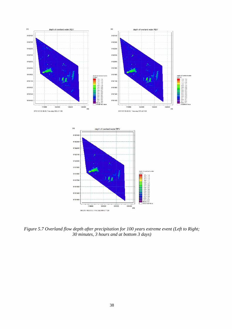
Right; 30 minutes, 3 hours and at bottom 3 days) .................................................................... 35 Figure 5.6 Water balance of 100 years extreme events for 2 weeks simulation ...................... 37 Figure 5.7 Overland flow depth after precipitation for 100 years extreme event (Left to Right;

30 minutes, 3 hours and at bottom 3 days) ............................................................................... 38

List of Tables

Table 2.1 Different Manning values of roughness coefficient (M) according to material type.

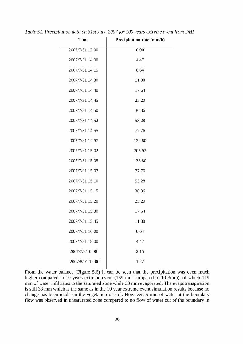
Adapted from French, 2007 ........................................................................................................ 8 Table 3.1 Illustration of different solutions mentioned in Figure 3.7 ....................................... 15 Table 4.1 Soil Profile ................................................................................................................ 27 Table 4.2 Swale definitions ...................................................................................................... 28 Table 4.3 Geological layers ...................................................................................................... 28 Table 4.4 Computational layers ................................................................................................ 29 Table 5.1 Precipitation data on 31st July, 2007 for 10 years extreme event from DHI ........... 33 Table 5.2 Precipitation data on 31st July, 2007 for 100 years extreme event from DHI ......... 36

1

1 Introduction

1.1 Background

The activities of man in many ways affected water cycle processes today. This is mainly

through the abstraction of water supply as well as creating an obstruction in the natural

rainfall cycle through the construction of impervious surfaces (Butler & Davies, 2004). For

example when rain falls, water should either evaporate or infiltrate into the soil however in

urban areas this is not the case. In urban areas there is barely any infiltration due to large

areas of the cities being paved (Villarreal & Bengtsson, 2005). It is this regard that Butler &

Davies (2004) contend that the above mentioned ways have led to the development of

different drainage systems (wastewater and stormwater) in urban areas. Urban drainage

systems, in particular, stormwater systems direct the flow of runoff and are expected to

prevent the flooding.

The stormwater system has gone through major changes in past decades (Malmö Stad, n.d.).

As a result of urbanization, open stormwater systems in urban areas are becoming more and

more popular and have been widely used in many cities all over the world. According to

Kleidorfer, et al. (2009), urbanization has had a huge impact on water resources which has

dramatically increased surface runoff. It was found that as a result of urbanisation there is a 20%

increase in rain intensity (Kleidorfer, et al., 2009). It is in this regard that open stormwater

systems are of paramount importance in this fast developing environment.

Augustenborg eco-city; one of Sweden´s largest urban sustainability projects, is renowned for

its sustainable urban planning, waste management as well as the effective open stormwater

systems (Malmö Stad, n.d.). Generally, the function of an open stormwater system can be

divided into four categories: infiltration, storage, detention and slow transport of runoff. In an

open stormwater system, rainfall runoff is handled by different types of open stormwater

system solutions e.g. green roofs, vegetated swales, open ditches and storage ponds.

Therefore, in order to improve and enhance the entire open stormwater system in

Augustenborg, a hydrological model was designed to evaluate the hydraulic performance of

these solutions.

1.2 Objectives

The objectives of the study are:

to evaluate the efficiency of the open stormwater system in Augustenborg eco-city for

improvement

to analyse predictability of potential flood under extremely high precipitation

conditions and suggest measures to deal with this risk

1.3 Aim

The aim of the study is to investigate the efficiency of the current open stormwater system on

the rate of flow during extreme climatic events.

1

2

1.4 Limitations

1. Uncertainties

Not all the data needed in the MIKE SHE model were able to be collected; therefore, several

assumptions were made e.g. the value of horizontal and vertical conductivity in both

saturated and unsaturated zone.

2

3

2 Presentation of fundamental components in the

study

2.1 Drainage systems

A group of researchers believed that the historical background of drainage systems date back

to many centuries ago (Cone, 2005). In the 18th

century in some urban areas; human waste

was harvested (used for fertiliser) and stormwater was reused for household activities. The

former method was abandoned due to the outbreak of disease whereas the latter was

developed into a more structured system (Chocat, et al., 2001). As time moved forward the

design of the conventional sewer system was designed and resulted in a modified version of

the water transport system we have today. Furthermore, in order to enhance the development

of drainage systems, the use of computer models became more prominent in the last century

(Butts, Payne & Overgaard, 2004).

On the contrary, Chocat et al. (2001) states, “…the latest developments in drainage

calculations are due not to technology but to philosophical realignments based on four

overriding concepts: a) introduction of sustainable development; b) acceptance of the

ecosystem approach to water resource management; c) impacts of drainage on receiving

waters; and d) recognition that complexity of the urban environment requires an integrated

approach.” It is in this regard that this thesis contends that combination of technological

advancements as well philosophical assumptions from the past hold ground for the better

management of drainage systems now as well as in the future.

Drainage systems are categorized into natural and conventional systems. Natural drainage

systems relate to drainage through infiltration and storage properties of semi natural features

(Ahmed, 2010). These features include; swales, ponds, detention basins etc. Conventional

drainage systems are the usual drainage of water through a piped network. There are two

types of conventional systems namely; combined and separate. Combined systems transport

wastewater and stormwater in the same pipe whereas separate systems have two different

pipes transporting the respective flows (wastewater and stormwater). In European countries,

the most prevalent system is the combined system whereas in Sweden only 15% of sewer

systems are combined with the rest separate (Berggren, 2007). In addition, the separate system

can be in a number of forms; piped, open, or a combination of these two. An open system usually

contains a combination of the following: ponds, channels, wetlands, green roofs, green infiltration

surfaces and porous paving (Ahmed, 2010). In a combined system; the pipe transporting water

is normally only 10% full and the rest is only used during the rainy season, meaning that is

almost never used to full capacity; this being its main disadvantage. Then, the advantage of

the separate system is that stormwater and wastewater do not mix, but due to two pipes, the

cost of construction is much higher.

The combination of drainage methods used brings up another interesting topic, in field of

water management, that no one facet can be considered as the best solution to proper drainage

but rather a combination of facets. So in order to achieve better drainage systems, future

research needs to focus also on specialised solutions (open stormwater systems) rather

general solutions (conventional system) or a combination of the two (Cone, 2005). On the

contrary, at times specialised solutions can be expensive and may not be able to be used in all

parts of the world e.g. developing countries. Thus, in developing countries, there is a need for

3

4

link between specialised solutions as well as generalized solutions to find a common ground

that is suitable to ensure sustainability.

Literature of the past few years shows a trend, showing that sustainability is taking priority in

terms of the development of drainage systems (Villarreal, Semadeni-Davies & Bengtsson,

2004). However, in its true sense much is left to be desired when it comes to standard of these

sustainable drainage systems. The major problem of the past of integrating design techniques

with ecological issues still prevails. With urbanization increasing at a very fast rate this

integration becomes paramount for the development of drainage systems. Steiner (2002)

believes that integrating human needs, design parameters as well as ecological factors need to

followed for better sustainability. He further goes on to argue that conventional methods need

to be upgraded to Best Management Practices (BMP’s). BMP’s are structural methods used

in the construction of stormwater systems. The synonym for BMP’s in Europe is Sustainable

Urban Drainage Systems (SUDS). One of the main goals of stormwater management systems

is to reduce the impacts of urban development on the movement of water in urban areas

(Scholes, Ellis & Revitt, 2007). In order to have full efficiency of these systems, stormwater

management systems can be designed in a series. This means that a series will comprise of a

number of components that will have its specific function. Some components will control

flooding, others water quality as wells as storage of runoff. Also, they will have value such

as: aesthetic and recreational benefits (Villarreal, Semadeni-Davies & Bengtsson, 2004).

More recently, stormwater management systems have been used to mimic real life natural

processes. This has been done with aids of sophisticated computer models such as the MIKE

SHE and MIKE URBAN models. These models will be discussed further later in this chapter.

An example of series components in a stormwater management system are described by a

“suburban retrofit” in Sweden; of which the exact location is not mentioned (Villarreal,

Semadeni-Davies & Bengtsson, 2004). Villarreal (2004) further suggests that an unnamed

report says that the system comprised of open channel which received water from

surrounding areas and a detention pond for storage of water. He further iterated that

stormwater management systems should perform at least more than one function to ensure

sustainability in all seasons. For example, aesthetics can be of huge benefit during dry periods

where human uses may conflict with open channel use. Like in the example in Sweden, the

major function of the stormwater system was only conveyance of water, which caused

residents to dislike the system. This resulted in litter collecting in the system; however that

was not the only reason for the litter. The litter was made visible also due to the displacement

of vegetation but overall the attitudes of residents was not good due to the fact the system had

only one purpose. Furthermore, (Mehler & Ostrowski, 1998) agrees with Villarreal,

Semadeni-Davies & Bengtsson (2004), that conventional stormwater systems are not able to

solve many complex issues relating to stormwater and water quality issues, thus better

stormwater systems such as BMP’s should be used.

Other BMP’s that have been deemed to be a solution to stormwater management are also

under the spotlight. Green roofs are a popular stormwater management system that is being

scrutinized carefully to assess their true effect on the retention of stormwater. In the past, roof

runoff was regarded as a source of clean drinking water, irrigation and other household uses.

However, according to past studies in Northern Europe much is left to be desired about the

quality of the runoff water (Good, 1993).There was an increase in the levels of zinc (from

galvanized roofs surfaces) in runoff water. Although the levels of zinc where low to harm

4

5

human health, it was harmful to aquatic life. This leaves room for research and investigations

into the storage possibilities of stormwater in areas where galvanized zinc roofs are still used.

On the other side of the coin, currently, the use of galvanized roofs across the world has been

reduced and concrete roofs are used, which negate the principle of reduction of runoff. The

response to this problem was then solved with the introduction of a green roof or also known

as a vegetated roof. Obviously, vegetated roofs which are slightly more expensive to

construct do perform the desired function of reducing the flow rate of runoff.

As has been discussed in this chapter, in order for better movement of water, the design of

stormwater management facilities need to be revised. Literature shows that stormwater

designs are improving but at a slow rate (Butler & Davies, 2004). Not only does the

advancement of design principles need to change but also the professionals involved in the

construction is vital in the implementation of better stormwater management systems.

Mihelcic, et al. (2003) states, “…together the mature fields of the physical sciences,

engineering, economics, and human behavioural studies to address the critical issues of

sustainability”, can go a long way in achieving sustainable stormwater solutions. It is in the

regard that the use of computer aided modelling software has become vital for future

development.

2.2 MIKE SHE

Hydrological modelling relates back to the late 60’s where proposed a blueprint for

modelling the hydrological cycle began (Freeze & Harlan, 1969). In this blueprint, flow

processes where described using derived partial differential equations. This made the model

very mathematical and complicated. Then in 1977, a consortium was formed between three

European organisations; Système Hydrologique Européen (SHE). These organisations used

Freeze & Harlan’s (1969) equations as a base to improve hydrological modelling. From this

was the emergence of several MIKE software.

MIKE SHE is an advanced integrated hydrological modelling software that is part of the

MIKE group of software owned and designed by the Danish Hydrological Institute (DHI)

(Refsgaard & Storm, 1995). It is based on deterministic and physically based modelling

systems, making its application in research very purposive (Abbott et al., 1986). The models

main function relates to the movement of water in relation to the hydrological cycle. So,

basically the model describes a number of hydrological processes e.g. interception,

evapotranspiration, overland and channel flow, flow in the unsaturated zone and saturated

zone, snow melt as well as the exchange of water between aquifers and rivers (Figure 2.1).

According to Butts, Payne & Overgaard (2004) the abovementioned processes can be

represented with different degree of emphasis depending ones goals of the study, the

availability of field data and the modeller’s choices.

5

6

Figure 2.1 Processes in MIKE SHE model Source: DHI

In order to describe these processes, MIKE SHE uses a number of equations to calculate

flow. For example partial equations are used in a number of processes namely: channel flow

(one dimensional Saint-Venant equation), overland (two-dimensional Saint-Venant equation),

unsaturated (one-dimensional Richard Equation) and saturated subsurface flows (three-

dimensional Boussinesq equation). Analytical methods are used in the model to describe

evaporation; interception and snow melt (DHI, 2004).

In addition, potential evapotranspiration, precipitation, elevation, soil type and cover, are

represented using network grids. Within each of the grids, vertical and horizontal layers are

described at a number of depths. This is seen as lateral flow between the grids which occurs

as overland flow or saturated flow. One assumption that is made when Richard Equation is

used is that horizontal flow is negligible in the unsaturated zone compared to the vertical

flow.

2.3 Open stormwater solutions

Decentralized open stormwater systems are becoming more and more popular in recent years

and are starting to be widely applied in small and rural communities where they can be most

cost-effective (National Small Flow Clearinghouse, 2000)

In Augustenborg, stormwater from roofs and other impervious surfaces is collected in gutters

and channelled on through canals, ditches, ponds before finally draining into a traditional

combined sewer system (VA SYD, n.d.).

6

7

In this section background on four main open stormwater solutions will be introduced and the

function of each will be discussed, focusing on the relevant aspects with regard to the

subsequent modelling steps. The four main open stormwater solutions includes: open channel

(ditches), green roofs, swales and storage ponds.

2.3.1 Open channel (ditches)

Open channels are a very important component in an open stormwater system and can be

categorized into two different types: natural and artificial channels. Artificial channels

include; irrigation canals, navigation canals, spillways, sewers, culverts and drainage ditches.

Open channels are usually constructed in a regular cross-section shape and are used for

diverting the flow stormwater, which in turn results in the decreasing the rainfall runoff peak

flow (Chow, 2009).

In order to know how much flow can be transported through an open channel or ditch, the

manning equation is usually used because it is simple and precise.

The Manning equation in the SI units system is defined as follows:

⁄

⁄ Equation 2.1

Whereby:

Q = flow rate (m3/s)

A = flow area (m2)

R = hydraulic radius (m)

M = Manning roughness coefficient

Sf = Friction Slope

According to equation 2.1, the flow rate is a function of flow area, hydraulic radius and

Manning resistance coefficient, however, Manning roughness, is very difficult to measure

directly in practice. The estimation of the roughness coefficient (Table 2.1) of the channel is

the most challenging task because different materials are used for lining the channel.

Generally, the value of Manning coefficient is estimated as the same value measured in

previous successful designs.

7

8

Table 2.1 Different Manning values of roughness coefficient (M) according to material type.

Adapted from French, 2007

Material Manning coefficient

Concrete (rough) 68

Concrete (smooth) 85

Plastic 80

Grass (lawn) 20

Cement mortar (neat) 90

Masonry 40

Rubble 30

2.3.2 Green Roofs

Different source control techniques have been applied in an open stormwater systems in order

to reduce the risk of flooding (Stahre, 2008). The primary goal is to decrease rainfall runoff

entering the combined sewer system which can be easily overloaded during high precipitation

seasons.

A green roof/vegetated roof (Figure 2.2), is a living surface of plants growing in a soil layer

on top of the roof (Stahre & Geldof, 2003). It is one of the most efficient solutions in open

stormwater systems aiming at reducing peak rainfall runoff flow (Stahre, 2008). Generally

there are 3 different types of green roofs; extensive, semi-intensive and intensive green roofs

depending on the depth of planting medium and the amount of maintenance they need

(Family Business Institute, n.d.). Extensive green roofs traditionally support 5-10 kilograms

of vegetation (drought resistant species) per square metre while intensive roofs support 35-70

kilograms of vegetation (trees and shrubs) per square metre and semi-intensive green roofs

support ranges between 10 to 35 kilograms of vegetation (herbs and meadow vegetation) per

square metre (Family Business Institute, n.d.).

Figure 2.2 Green roof Structural Model (Peck, et al., 2009)

8

9

2.3.3 Swales

A swale is a vegetated open channel, planted with a combination of grasses and other

herbaceous plants (City of Indianapolis, n.d.). A swale can slow down the rapid flow of

stormwater runoff by ponding water between its loping sides. Ponding not only slows the rate

of flow but also separates pollutants from storm water. Once the swale becomes full, the

excess water will overflow over berms and flow into the main long ditches.

Swales have been used for runoff control from rural highways and residential streets for

many years, besides; they also provide infiltration and water quality treatment. As an efficient

open system solution, swales are becoming more and more popular because they can look

more aesthetically than a rock-lined drainage system and are generally simple to construct

and maintain (City of Indianapolis, n.d.).

2.3.4 Storage ponds

Storage ponds are usually used to slow the rainfall runoff by ponding a certain volume of

water performing as a detention container (Akan, 1993). The advantages of storage ponds are

mainly the following aspects:

reduce the peak flow downstream

reduce the erosion led to sewage system through sedimentation process

help to reduce the pollutant through setting particles

The routing equation is generally used for calculating the outflow for a specific reservoir,

especially for a pond (Akan, 1993).

Equation 2.2

Whereby: I is the inflow rate

O is the outflow rate

S is the water volume in storage pond

t is the time

9

10

10

11

3 Description Augustenborg Eco-city

3.1 Description of study area

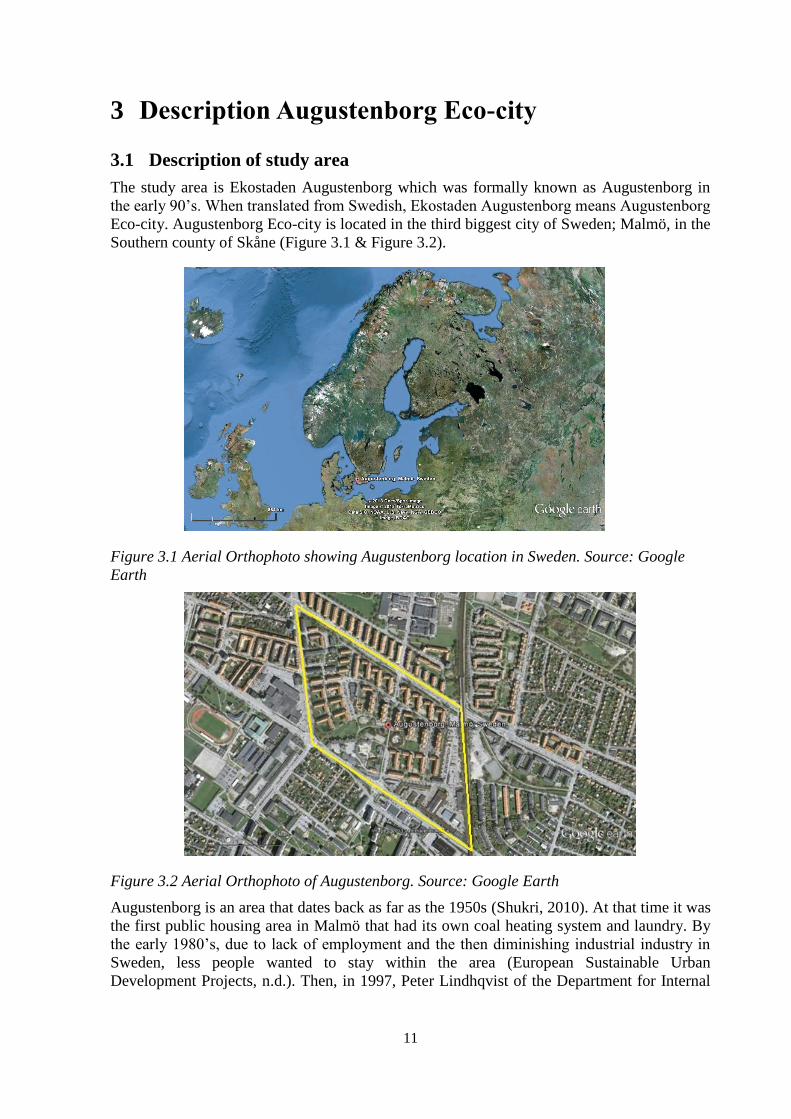
The study area is Ekostaden Augustenborg which was formally known as Augustenborg in

the early 90’s. When translated from Swedish, Ekostaden Augustenborg means Augustenborg

Eco-city. Augustenborg Eco-city is located in the third biggest city of Sweden; Malmö, in the

Southern county of Skåne (Figure 3.1 & Figure 3.2).

Figure 3.1 Aerial Orthophoto showing Augustenborg location in Sweden. Source: Google

Earth

Figure 3.2 Aerial Orthophoto of Augustenborg. Source: Google Earth

Augustenborg is an area that dates back as far as the 1950s (Shukri, 2010). At that time it was

the first public housing area in Malmö that had its own coal heating system and laundry. By

the early 1980’s, due to lack of employment and the then diminishing industrial industry in

Sweden, less people wanted to stay within the area (European Sustainable Urban

Development Projects, n.d.). Then, in 1997, Peter Lindhqvist of the Department for Internal

11

12

Services, Bertil Nilsson; former headmaster at the school in Augustenborg, and Christer

Sandgren of MKB (Malmö´s public housing company), came together and formed a coalition

suggesting the development of an eco-friendly industrial park (Ekostaden Augustenborg,

n.d.). Among many other reasons; deterioration of the buildings as well as basement flooding

was the major factors that led to suggestions of renovation and creation of the eco-friendly

industrial park. It is 1997 that Augustenborg received its current name of Ekostaden

Augustenborg and development of the Eco-city started in 1998 and was completed in 2002.

Currently, its area covers approximately 32 hectares and has a total population of about 3000

people (Shukri, 2010). Within this area other than a residential area, there are a number of

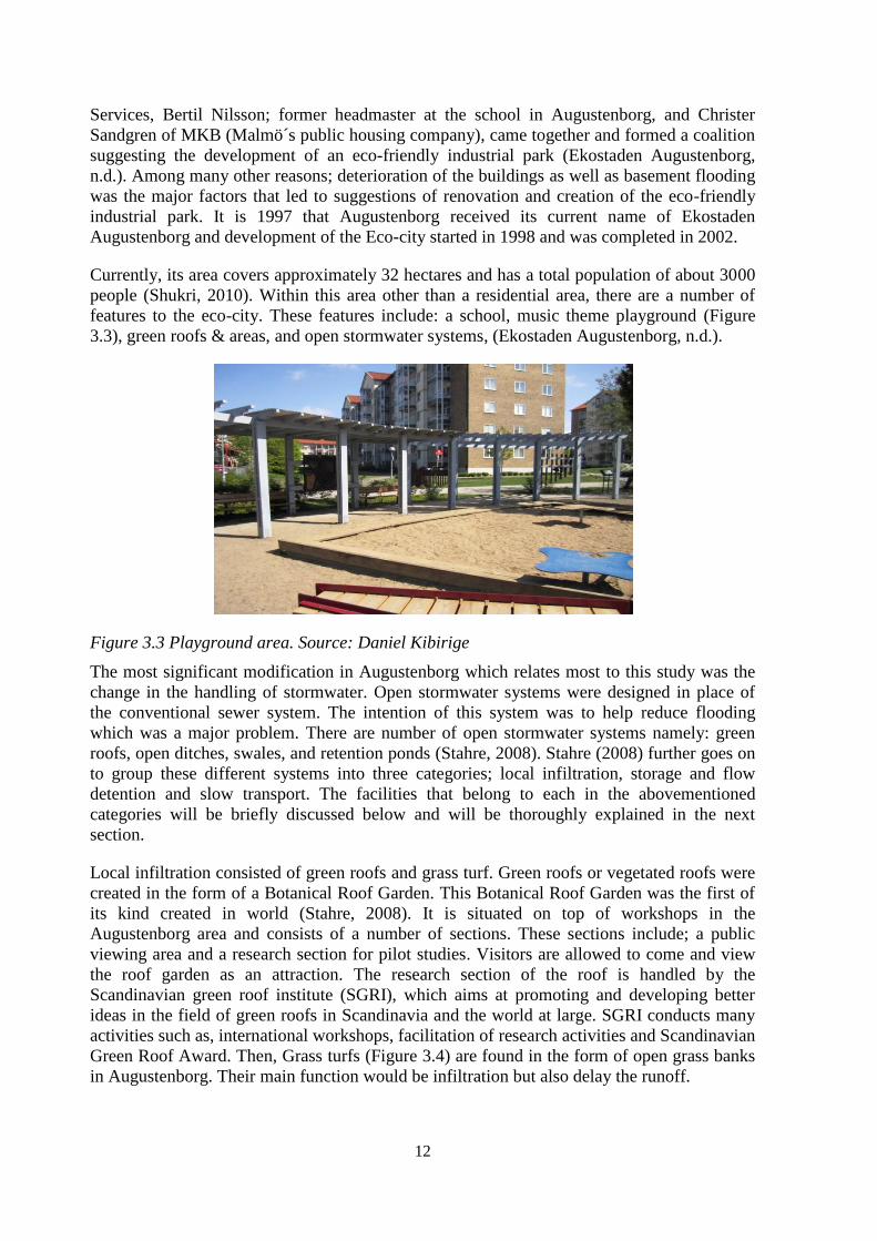
features to the eco-city. These features include: a school, music theme playground (Figure

3.3), green roofs & areas, and open stormwater systems, (Ekostaden Augustenborg, n.d.).

Figure 3.3 Playground area. Source: Daniel Kibirige

The most significant modification in Augustenborg which relates most to this study was the

change in the handling of stormwater. Open stormwater systems were designed in place of

the conventional sewer system. The intention of this system was to help reduce flooding

which was a major problem. There are number of open stormwater systems namely: green

roofs, open ditches, swales, and retention ponds (Stahre, 2008). Stahre (2008) further goes on

to group these different systems into three categories; local infiltration, storage and flow

detention and slow transport. The facilities that belong to each in the abovementioned

categories will be briefly discussed below and will be thoroughly explained in the next

section.

Local infiltration consisted of green roofs and grass turf. Green roofs or vegetated roofs were

created in the form of a Botanical Roof Garden. This Botanical Roof Garden was the first of

its kind created in world (Stahre, 2008). It is situated on top of workshops in the

Augustenborg area and consists of a number of sections. These sections include; a public

viewing area and a research section for pilot studies. Visitors are allowed to come and view

the roof garden as an attraction. The research section of the roof is handled by the

Scandinavian green roof institute (SGRI), which aims at promoting and developing better

ideas in the field of green roofs in Scandinavia and the world at large. SGRI conducts many

activities such as, international workshops, facilitation of research activities and Scandinavian

Green Roof Award. Then, Grass turfs (Figure 3.4) are found in the form of open grass banks

in Augustenborg. Their main function would be infiltration but also delay the runoff.

12

13

Figure 3.4 Open grass banks. Source: Xing Tan

Storage and flow detention in Augustenborg are in the form ponds and temporary storage

facilities. Storage ponds range in size and are located all around the study area (Figure 3.5).

,

Figure 3.5 Storage ponds. Source: Daniel Kibirige

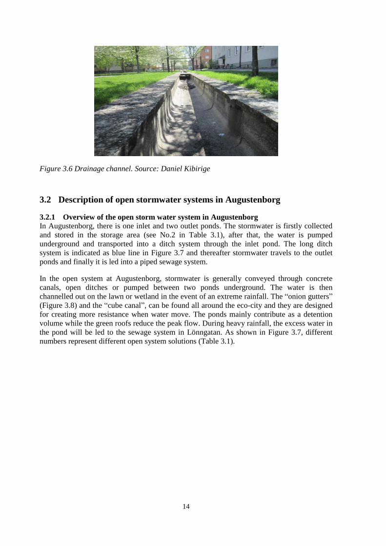
Slow transport facilities are found in different “drainage corridors”. A drainage corridor can

be seen in Figure 3.6 and is from the southeast to the southwest corner of the study area

(Stahre, 2008). They are in the form of concrete drainage canals, concrete cube canals,

vegetated cannels.

13

14

Figure 3.6 Drainage channel. Source: Daniel Kibirige

3.2 Description of open stormwater systems in Augustenborg

3.2.1 Overview of the open storm water system in Augustenborg

In Augustenborg, there is one inlet and two outlet ponds. The stormwater is firstly collected

and stored in the storage area (see No.2 in Table 3.1), after that, the water is pumped

underground and transported into a ditch system through the inlet pond. The long ditch

system is indicated as blue line in Figure 3.7 and thereafter stormwater travels to the outlet

ponds and finally it is led into a piped sewage system.

In the open system at Augustenborg, stormwater is generally conveyed through concrete

canals, open ditches or pumped between two ponds underground. The water is then

channelled out on the lawn or wetland in the event of an extreme rainfall. The “onion gutters”

(Figure 3.8) and the “cube canal”, can be found all around the eco-city and they are designed

for creating more resistance when water move. The ponds mainly contribute as a detention

volume while the green roofs reduce the peak flow. During heavy rainfall, the excess water in

the pond will be led to the sewage system in Lönngatan. As shown in Figure 3.7, different

numbers represent different open system solutions (Table 3.1).

14

15

Figure 3.7 Overview of the stormwater system in Augustenborg (VA SYD, n.d)

Table 3.1 Illustration of different solutions mentioned in Figure 3.7

Number Implication Number Implication

1 The Augustenborg botanical

roof garden area

9 Basketball court, storm water

collected here travel to 10

2 Storm water storage pumped

underground from storage area

10 Ditch through the park

3 Concrete canal 11 Outlet pond Nr 1

4 Wetland 12 Storage pond

5 Onion gutters 13 Macadam-bottomed ditch

6 Storage pond 14 Storage pond

7 Block flat with green roof 15 Constructed tone canal

8 Cube canal 16 Outlet pond Nr 2

15

16

3.2.2 Open channel

According to a report by International Green Roof Institute, an open drainage system, in the

form of a shallow ditch, was constructed across the park area in Augustenborg in order to

reduce the rainfall runoff speed (Figure 3.8), (Stahre & Geldof, 2003).

Figure 3.8 Shallow channel. Source: Daniel Kibirige

The swale is mostly filled up during wet weather conditions and during dry weather

conditions the drainage ditch and banks is dry. It is obvious that an open channel can be

easily integrated in the park environment and the other advantage is that the construction cost

is low (Stahre & Geldof, 2003).

3.2.3 Green roof

In Augustenborg residential area, a vegetation cover of sedum grass on top of 9,500 m2 of the

roofs is applied in order to reduce the stormwater runoff, and in Augustenborg Botanical

Roof Garden, the green roofs reduce about 50% of the annual runoff (Stahre, 2008). A

section of the green roof installation at Augustenborg eco-city is shown in Figure 3.9.

Figure 3.9 Green roof installation at Augustenborg eco-city. Source: Daniel Kibirige

The green roofs can be applied in those housing estates where most of the buildings had a flat

roof, and those applied green roofs managed to reduce the stormwater runoff from the roofs

efficiently (Figure 3.9). They also played a role as an effective insulation for the buildings.

16

17

The green roofs also contribute as saving energy for heating system and protect the roof

construction.

3.2.4 Swales

In Augustenborg, artificial swales can be found all around and are designed to manage

rainfall runoff, filter pollutants and increase rainfall infiltration. The constructed swales are

generally low tract of land connected to an open channel or constructed canal. When it rains,

the rainfall runoff will firstly reach the swale, at the point where stormwater begins to

infiltrate into the ground. If the soil is saturated as a result of heavy rain, the excess runoff

will flow downwards along the slope of the swale and finally into the open channel. As

mentioned in open channel section, the canals are designed to accommodate wet weather

conditions whereas during dry weather conditions they are totally dried out. Conversely, the

swale system plays an important role especially during dry weather conditions, most of

stormwater infiltrates downward from the swale land instead of being transported to the open

channel system.

3.2.5 Storage ponds

In order to be able to handle stormwater from the residential area as well as garden parts of

Augustenborg, large detention volumes are required. The best solution was to build several

storage ponds for the excess stormwater during heavy rainfall season. In Augustenborg, the

main function of storage ponds is to delay the peak flow by storing a certain volume of

stormwater in the ponds, thus reducing the peak flow. They can also help reduce pollutant

from stormwater through sedimentation (Akan, 1993); as a result, the sewer system and

treatment plant will receive less pollutant than usual.

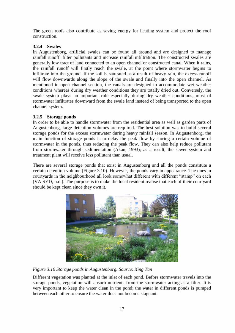
There are several storage ponds that exist in Augustenborg and all the ponds constitute a

certain detention volume (Figure 3.10). However, the ponds vary in appearance. The ones in

courtyards in the neighbourhood all look somewhat different with different “stamp” on each

(VA SYD, n.d.). The purpose is to make the local resident realise that each of their courtyard

should be kept clean since they own it.

Figure 3.10 Storage ponds in Augustenborg. Source: Xing Tan

Different vegetation was planted at the inlet of each pond. Before stormwater travels into the

storage ponds, vegetation will absorb nutrients from the stormwater acting as a filter. It is

very important to keep the water clean in the pond; the water in different ponds is pumped

between each other to ensure the water does not become stagnant.

17

18

18

19

4 Materials and Methods

This study involved the design of a hydrological model. A MIKE SHE model was created to

simulate the flow of water during extreme climatic events.

4.1 Data collection of study area

Data about Augustenborg eco-city was collected from a number of sources namely: Malmö

municipality, VA SYD, Sveriges Geologiska Undersökning (SGU); known as Geological

Survey of Sweden, internet and literature. The data collected included: location data,

topography data, land use map, soil map, meteorological data (rainfall and temperature).

4.2 Field investigations

A number of visits to Augustenborg eco-city were done in person to check the precise

location of open stormwater solutions.

4.3 Detailed description of MIKE SHE Model

4.3.1 Introduction

The principles behind the creation of the MIKE SHE model for Augustenborg used in this

study will be discussed in this chapter. Particular reference will be made to parts relating to

the modelling of the open stormwater solutions. There are seven different components in the

model. These components include: model domain and grid, topography, climate, land use,

overland flow, unsaturated flow and saturated zone (Figure 4.1). Of the seven much emphasis

will be placed on components that relate to water movement that are specified in the model

which include; overland flow (OL), evapotranspiration (ET).

Figure 4.1 Schematic layout of MIKE SHE model

Model Domain & Grid

• GIS to MIKE Grid

Topography • Digital Elevation

Model

Climate

• Temperature

• Precipitation

• Reference Evapotranspiration

Landuse •

Vegetation

Overland Flow

• Manning number

• Detention storage

• Initial water depth

• Subsurface leakage coefficient

Unsaturated Zone

• Soil profile definition

Saturated Zone

• Geological layers

• Computational layers

•Drainage

20

4.3.2 Model domain and Grid

Augustenborg is located in the southeast part of Malmö Municipality with the coordinates of

55° 34′ 47″ N, 13° 1′ 29″ E. The eco-city is surrounded by roads to its north, west and south

and a railway to its east. Therefore, the roads and railway constituted as fixed head

boundaries which prevented inflow from surrounding areas. These boundaries were then used

for both the surface water and groundwater components in the model.

Before setting up a hydrological model for a specific area, it is important to describe the

boundary. Therefore the first step was to define the model area. The boundaries of the model

were roughly chosen due to constraints in data. It was assumed that the boundaries of surface

water were defined not to allow the inflow of water from surrounding areas. As for the

groundwater ideally a larger area would have been used as the surface and groundwater do

not coincide due to lack of data covering a larger area; the same boundary conditions as in

surface water were used.

Initially, in this case, a xyz ASCII file containing local elevation data in Augustenborg was

interpolated to the a “MIKE grid” by using MIKE SHE TOOLBOX and the catchment is

defined by creating a Dfs2 file from a shape file. As shown in Figure 4.2 the blue area shows

the defined geometric area in the model and boundary of the whole Augustenborg eco-city as

well as its absolute location.

Figure 4.2 Design of boundary in Augustenborg, in MIKE SHE model

4.3.3 Topography

In MIKE SHE application, topography was generated by using elevation data (shown as

black dots in Figure 4.3) obtained from Malmö stad and based on the topography data the

upper boundary of the model was defined. Figure 4.3 shows the Digital Elevation Model

(DEM) for the area with the elevation corrected for all buildings. In the model, the elevation

of all buildings was raised to 1 m higher than ground surface to indicate to the model that

water should flow around the building and not infiltrate into them. Elevation is highest in the

Southeast area and lowest in Northwest and in the Eastern area it is over 20.8 m (shown in

red).

20

21

Figure 4.3 Model area of Augustenborg

Topography (Figure 4.3) is usually defined through a DEM either as a point theme shape file,

or an ASCII file (DHI, 2012). In this case, an ASCII file containing the elevation data of

Augustenborg was converted to a dfs2 file by using the MIKE ZERO TOOLBOX.

4.3.4 Climate

The climate in Malmö can be classified as mild and oceanic regardless of its northern

location compared to other coastal cities in Europe. The maximum temperature during

summer ranges from 18 to 21C and minimum temperature varies between 10 and 12C; with

the rare occasion of +25C (Figure 4.4). Winter temperatures vary from season to season but

on average the temperatures are between -3 and -4C with the odd day of winter reaching

temperatures of -10C (Climate Zone, 2004). Also, in the winter season; snow falls during the

months of December to March. Rainfall in this region is moderate throughout the year and an

average of 600 mm of rainfall per year is recorded. The driest months of the year are from

January till June which usually record less than 50 mm per month. The second half of the

year has more rainfall; at times in access of 100 mm per month.

21

22

Figure 4.4 Daily mean air temperature (2007)

In MIKE SHE, climate section is made up of four different parts including: precipitation,

reference evapotranspiration, air temperature and snow melt.

The precipitation rate, reference evapotranspiration and air temperature were all specified by

dfs0 files created for each respective section. Precipitation data from 2000 to 2011 was used

for creating the precipitation rate curve however emphasis was placed on the years 2006-

2008. Average monthly evapotranspiration (Figure 4.5) data from January to December was

used and repeated for the years 2001 to 2011.

Figure 4.5 Monthly potential evapotranspiration

In MIKE SHE model, the evapotranspiration processes were separated and modelled in

different processes (DHI, 2012): Firstly, some of the rainfall runoff is intercepted by the

vegetation canopy, from which part of the storm water evaporates. The remaining water

travels to the soil surface, and contributes as either surface runoff or percolates into the

-10

-5

0

5

10

15

20

25

1/1

/20

07

2/1

/20

07

3/1

/20

07

4/1

/20

07

5/1

/20

07

6/1

/20

07

7/1

/20

07

8/1

/20

07

9/1

/20

07

10

/1/2

00

7

11

/1/2

00

7

12

/1/2

00

7

Tem

pe

ratu

re (

°C)

Month

0

20

40

60

80

100

120

140

1 2 3 4 5 6 7 8 9 10 11 12

Po

ten

tial

Eva

po

tran

spir

atio

n

(mm

/mo

nth

)

Month of the year

22

23

unsaturated zone. Some of the infiltrating water will be evaporated from the higher parts of

the roots zone or will be transpired by the vegetation roots. The remainder of the infiltrating

water will be recharged to the groundwater and stored in the saturated zone.

MIKE SHE uses the Crop Reference Evapotranspiration rate for all calculations of

Evapotranspiration and was calculated as follows:

Equation 4.1

Where

ETref is the Reference Evapotranspiration

Kc is the Crop Coefficient specified in the Vegetation Development Table that adjusts the

Reference ET rate for different vegetation types.

The maximum amount of ET that can be removed within one time step is

Equation 4.2

Recent 15 years temperature data was collected from SMHI and latest 11 years data was

selected for setting up a df0 file in MIKE SHE. The mean temperature value was then used as

the daily temperature values and inserted in MIKE SHE model. Precipitation data was

collected from VA SYD while evapotranspiration data was provided by DHI.

When referring to the snow melt section, the value of degree-day coefficient (amount of

water that melts per day) was set to 2 mm/C/day as a constant distribution while the values

of other parts e.g. melting temperature, min snow storage, max wet snow fraction, initial total

snow storage and initial wet snow fraction are all set to 0.

4.3.5 Land Use

The land use in Augustenborg comprises of residential buildings, a school, musical

playground, trees, open lawn, wetlands and open stormwater solutions (green roofs, open

ditches, swales etc.). The newly built school building with natural materials, ground source

heat pump and solar thermal panels is located in the northern part of the eco-city.

4.3.6 Vegetation

Vegetation affects the hydrological cycle mainly through evapotranspiration, which is the

sum of evaporation and plant transpiration from the Earth's land surface to atmosphere.

Evaporation accounts for the movement of water to the air from soil and Transpiration

accounts for the movement of water within a plant and the subsequent loss of water as vapour

through stomata in its leaves. Evapotranspiration is an important part of the water cycle

therefore the vegetation factor should be defined properly in MIKE SHE.

In the MIKE SHE model, vegetation properties were set same over the whole area.

Vegetation properties were used to calculate the actual evapotranspiration from crop

reference evapotranspiration defined under climate section which was discussed previously

(DHI, 2012).

23

24

The key vegetation properties are Leaf Area Index (LAI) and Root Depth (RD). Generally the

LAI and Root Depth can be specified directly as a time series. Otherwise, they could be

defined as a crop cycle in the vegetation properties editor.

Necessary information on LAI and RD can be found from the agronomy department at local

university or relevant government sector (Yan, et al., 2012). In this case, the data type of

vegetation was selected as vegetation property file from which almost all the vegetation types

could be found. Figure 4.6 shows the vegetation properties of a mix of grass, bushes and trees

in Augustenborg.

Figure 4.6 The key vegetation properties are Leaf Area Index (LAI as shown in blue line) and

Root Depth (RD as shown in red line)

For each crop stage, three vegetation parameters needed to be specified (DHI, 2012):

1. LAI - The Leaf Area Index was defined as the area of leaves per area of ground surface.

This can vary between 0 and 7 depending of the vegetation type and the values of LAI are

widely available in the literature for most main plant types.

2. RD - The Root Depth of the crop was defined as the depth below ground in millimetres to

which roots extend (Allen, 1998). It usually changes from season to season. The soil type was

taken into consideration since some crops might develop different root distribution upon the

characteristics of soil.

3. Crop coefficient (Kc) - The crop coefficient adjusts the Reference ET rate relative to the

actual evapotranspiration for different vegetation types (DHI, 2012). Since most crops may

differ one has to consider two situations namely quoted in DHI (2012):

“In the early crop stages, where LAI of the farm crop is lower than the LAI of the

reference grass crop, the evapotranspiration of the farm crop is less then the calculated

reference evapotranspiration. This is accounted for in the Kristensen & Jensen ET

calculation, since a crop LAI is used as input. Therefore, for most field crops it is

therefore not necessary to specify Kc values below 1 in the early crop stages.”

24

25

“In the crop mid-season the opposite situation may occur where crop potential

evapotranspiration is larger than the calculated reference evapotranspiration of the

reference grass crop. This is not handled in the ET calculations, and Kc values above

1 may therefore be relevant for some crops in the mid-season during the period where

crop leaf area index is at its maximum.”

A value of 1 was chosen in this simulation. This meant that the assumption was made that the

maximum evapotranspiration rate will equal the reference evapotranspiration rate.

4.3.7 Overland flow Overland flow over Augustenborg area varies depending on the season as well as the

occurrence of an extreme climatic event. Generally the movement of water is channel through

different stormwater systems. Infiltrations occurs on permeable areas such as swales, green

roofs and open banks whereas asphalt and concrete surfaces allow the flow of water in a

controlled and safe manner.

The finite difference method was selected to simulate overland flow. It can be seen there are

several items required for calculation processes and these items are included in the main

dialogue of the model for overland flow. There items include:

1. Manning number, is equivalent to the Stickler roughness coefficient,

2. Detention Storage, is used to limit the amount of water that can flow over the ground

surface,

3. Initial Water Depth on the ground surface, is used for the overland flow calculations and

the initial water depth is usually set to 0,

4. Surface-Sub surface leakage coefficient.

Surface-subsurface leakage coefficient reduces the infiltration rate at the ground surface by

reducing both the infiltration rate and the seepage outflow rate across the ground surface

(DHI, 2012). Figure 4.7 show that all the buildings represented an impervious surface (in

blue), which meant the vertical hydraulic conductivity was very limited (close to 0).

25

26

Figure 4.7 Impervious area shown in blue in Augustenborg

The value of the leakage coefficient was set to zero for all buildings as water cannot infiltrate

through the buildings and the rest of the area was set to have full contact to the UZ/SZ zones.

4.3.8 Unsaturated Flow

Unsaturated zone is the area where some of the pores are filled with water. It is directly under

the top surface that accounts for percolation of water that has been infiltrated through the top

layer of soil. The flow of water in this zone is vertical as most of it is flowing downwards into

the saturated zone. The depth of the unsaturated zone is dependent on the level of the water

table. The water table is the border line between the unsaturated zone and the saturated zone.

In MIKE SHE there are three methods that are used to calculate unsaturated flow. These

methods include Richards’s equation, the gravity flow and the two-layer water balance. In

this instance Richards equation was used which was specified in the simulation specification

dialog. Richards equation is quoted by DHI (2012) as the, “driving force for transport of

water in the unsaturated zone is the gradient of the hydraulic head, h, which includes a

gravitational component, z, and a pressure component, . This equation is shown below:

( ) (

) Equation 4.3

Where,

K; is the hydraulic conductivity

is the pressure head

z; is the elevation

26

27

θ is the water content

t; is time

Furthermore, Pachepsky (2003) contends the Richards’ equation is the most often used in

modelling of water transport. Its application has been easy and widely used in the calculation

of unsaturated flow conditions, hence its selection for use in our model.

In this simulation the method of classification that was chosen from the model dialogue was

“Calculated in all Grid points”. This option was chosen as it is recommended for smaller

scale studies, or studies where the classification system becomes intractable, which in our

case, it’s a smaller scale study.

4.3.9 Soil profile definition

In this model the unsaturated flow is represented by the definition of the soil profile. The

dominant soil covering layer in Augustenborg is till (Figure 4.). The till was divided in to

vertical layers, the upper more permeable than the lower. A topsoil (Matjord) layer was added

to the geological description (Table 4.1 and Table 4.2). Table 4.2, displays the geological

description of swales in the model.

Figure 4.8 Soil profile definitions

Table 4.1 Soil Profile

From depth To depth Soil type

1 0 m 0.3 m Matjord 0

2 0.3 m 2 m Coarse Till (0-0.5 m)

3 2 m 5 m Coarse Till (0.5-2 m)

Note: The Matjord, was inserted as a top layer of soil.

1

0

Undefined Value

119664 120340

[meter]

6161400

6161500

6161600

6161700

6161800

6161900

6162000

6162100

6162200

6162300

[meter]

27

28

Table 4.2 Swale definitions

From depth To depth Soil type

1 0 m 0.3 m Matjord 0

2 0.3 m 2 m Gravel

3 2 m 5 m Coarse Till (0,5-2 m)

4.3.10 Saturated Zone

The saturated zone is the area where all the pores are completely filled with water. When

water enters this zone it is classified as groundwater. The top of this zone is called the water

table and is the boundary between it and the unsaturated zone.

The creation of the saturated zone in the MIKE SHE is based on 3D Finite Difference

Method which involves defining the geological model, vertical numerical discretisation,

initial conditions and boundary conditions.

The MIKE SHE Graphical User interface shows that the initial conditions are defined as a

property of numerical layer whereas the geological models as well as the vertical

discretisation are independent. The boundary conditions such as wells, drains and rivers are

also defined independently.

4.3.10.1 Geological layers

Geological layers were created using the layers that were discussed in the unsaturated zone.

In each layer, lower level, horizontal and vertical hydraulic conductivity, specific yield and

storage where chosen. This is shown in Table 4.3:

Table 4.3 Geological layers

The lower level values define the bottom of geological layers relative to the ground hence

their negative values. The hydraulic conductivities are a function of soil texture and are

related to the ease with which water flows through the soil (DHI, 2004). This mean that

compacted soil have a lower conductivity unlike loose, coarse soils (DHI, 2004) and (Fetter,

2000).

Soil Layers

Lower level Kh Kv Specific Yield Storage

Matjord -0.3 1e-006 1e-006 0.2 0.0001

Course Till 0-0.5 -2 2e-005 5e-006 0.2 0.0001

Course Till 0.5-2 -5 1e-006 1e-007 0.2 0.0001

28

29

4.3.10.2 Drainage

Drainage in the MIKE model was set based on permeability. Most areas in the study area are

permeable due to the open stormwater solutions. The areas that are not permeable are

concrete ditches, parking places and buildings. In MIKE SHE, the areas where buildings are

were set to -1.7 m relative to the ground taking into account the geological layering of soil.

Other areas where set to zero indicating that water would be able to infiltrate into those areas.

4.3.10.3 Computational layers

Of the three geological layers, it was decided to make two computational layers. The first two

layers (Matjord and Course Till 0-0.5 m) were combined into one layer and the bottom layer

(Course Till 0.5-2 m) was left as a layer on its own (Table 4.4) in order to represent the

separate soil layers.

Table 4.4 Computational layers

Computational Layers Lower level Initial Potential Head

L1 -2 -1.5

L2 -5 -1.5

4.3.11 Calibration data

In this study there was no observed data which meant that there it was no calibration and

validation to compare the results of the model.

4.4 Description of open stormwater solutions in MIKE SHE model

In MIKE SHE, all the open solutions including storage ponds (Figure 4.3), swales and open

channel are properly defined as shown in, Figure 4.9 and Figure 4.10. Green roofs were not

defined in MIKE SHE because the large amount of rainfall cannot be handled by green roofs

in other words; the capacity of green roofs for handling stormwater is limited thus they were

ignored in MIKE SHE model.

29

30

Figure 4.9 Swales area defined in red

Figure 4.10 Long open ditch system (blue line) is defined around the buildings

30

31

5 Results

This chapter presents efficiency of the open stormwater systems in Augustenborg eco-city

and the predictability flooding under extremely high precipitation conditions. The results are

presented in three simulation scenarios namely: 1year prediction of hydrological balance, 10

year extreme rainfall event and 100 year extreme rainfall event. The main focus of the results

in all three scenarios will be based on water balances i.e. a reasonable amount of

evapotranspiration and overland flow (runoff) since there was no calibration data to compare

the model results.

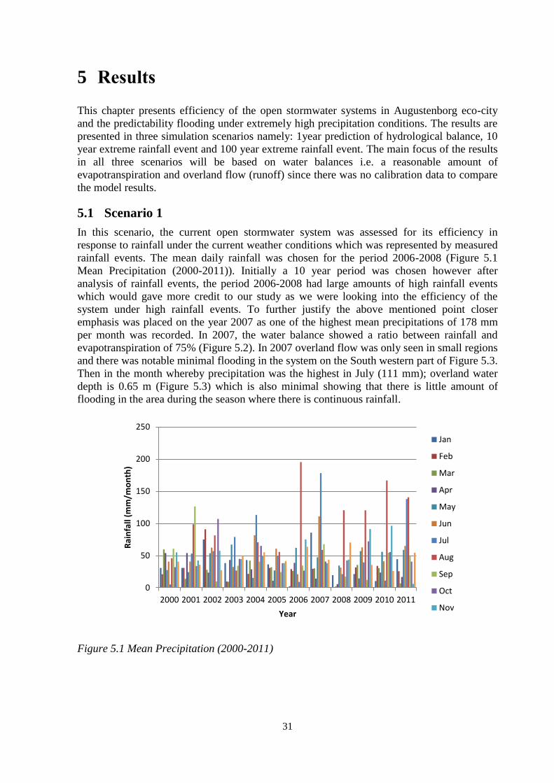
5.1 Scenario 1

In this scenario, the current open stormwater system was assessed for its efficiency in

response to rainfall under the current weather conditions which was represented by measured

rainfall events. The mean daily rainfall was chosen for the period 2006-2008 (Figure 5.1

Mean Precipitation (2000-2011)). Initially a 10 year period was chosen however after

analysis of rainfall events, the period 2006-2008 had large amounts of high rainfall events

which would gave more credit to our study as we were looking into the efficiency of the

system under high rainfall events. To further justify the above mentioned point closer

emphasis was placed on the year 2007 as one of the highest mean precipitations of 178 mm

per month was recorded. In 2007, the water balance showed a ratio between rainfall and

evapotranspiration of 75% (Figure 5.2). In 2007 overland flow was only seen in small regions

and there was notable minimal flooding in the system on the South western part of Figure 5.3.

Then in the month whereby precipitation was the highest in July (111 mm); overland water

depth is 0.65 m (Figure 5.3) which is also minimal showing that there is little amount of

flooding in the area during the season where there is continuous rainfall.

Figure 5.1 Mean Precipitation (2000-2011)

0

50

100

150

200

250

2000 2001 2002 2003 2004 2005 2006 2007 2008 2009 2010 2011

Rai

nfa

ll (m

m/m

on

th)

Year

Jan

Feb

Mar

Apr

May

Jun

Jul

Aug

Sep

Oct

Nov

31

32

Figure 5.2 Water Balance (2007)

Figure 5.3 Depth of Overland Flow (2007)

5.2 Scenario 2

In order to evaluate any water system it is essential to assess the risk of flooding in the area.

In this scenario the system in Augustenborg was put under a 10 year extreme rainfall event

which takes place on the 31st of July, 2007. A total of two weeks were simulated; one week

32

33

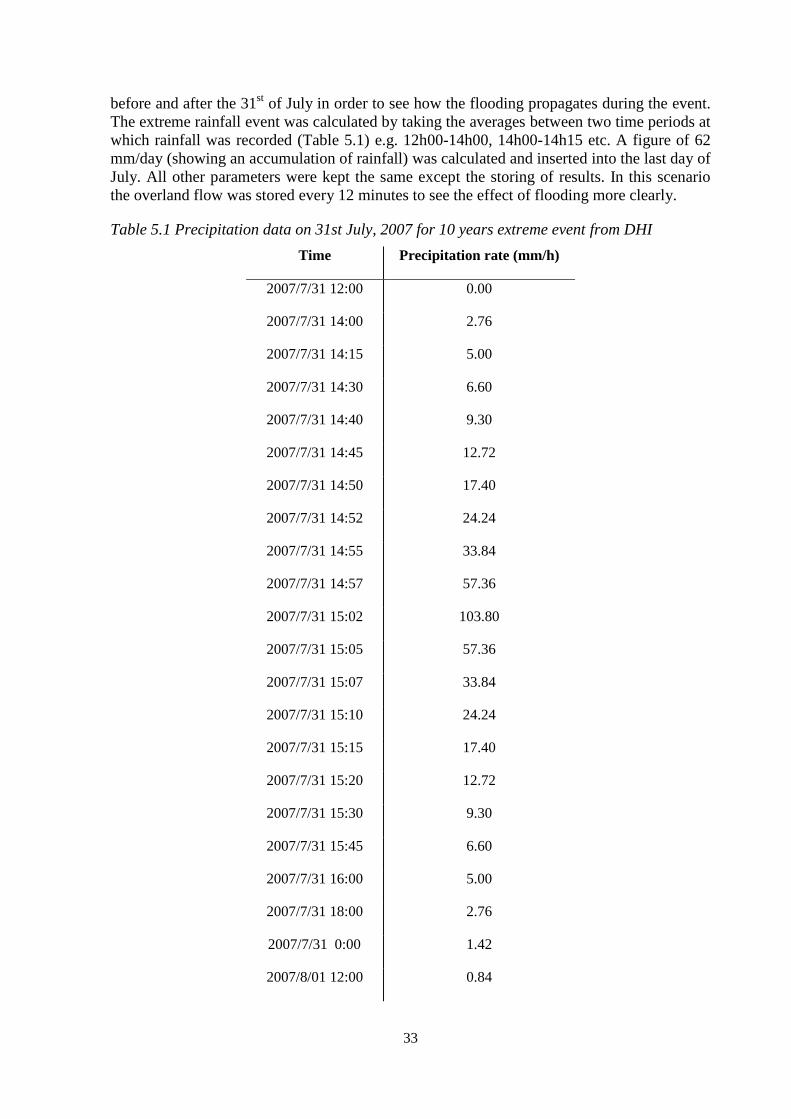
before and after the 31st of July in order to see how the flooding propagates during the event.

The extreme rainfall event was calculated by taking the averages between two time periods at

which rainfall was recorded (Table 5.1) e.g. 12h00-14h00, 14h00-14h15 etc. A figure of 62

mm/day (showing an accumulation of rainfall) was calculated and inserted into the last day of

July. All other parameters were kept the same except the storing of results. In this scenario

the overland flow was stored every 12 minutes to see the effect of flooding more clearly.

Table 5.1 Precipitation data on 31st July, 2007 for 10 years extreme event from DHI

Time Precipitation rate (mm/h)

2007/7/31 12:00 0.00

2007/7/31 14:00 2.76

2007/7/31 14:15 5.00

2007/7/31 14:30 6.60

2007/7/31 14:40 9.30

2007/7/31 14:45 12.72

2007/7/31 14:50 17.40

2007/7/31 14:52 24.24

2007/7/31 14:55 33.84

2007/7/31 14:57 57.36

2007/7/31 15:02 103.80

2007/7/31 15:05 57.36

2007/7/31 15:07 33.84

2007/7/31 15:10 24.24

2007/7/31 15:15 17.40

2007/7/31 15:20 12.72

2007/7/31 15:30 9.30

2007/7/31 15:45 6.60

2007/7/31 16:00 5.00

2007/7/31 18:00 2.76

2007/7/31 0:00 1.42

2007/8/01 12:00 0.84

33

34

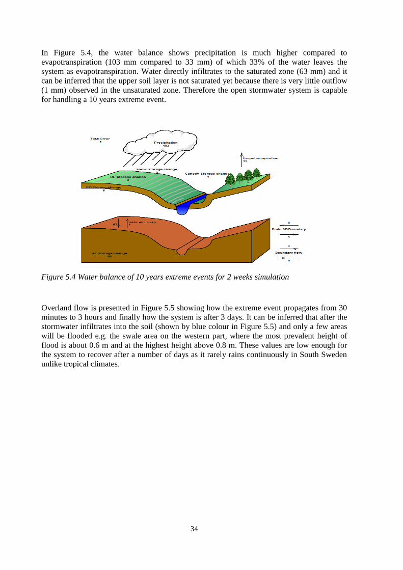
In Figure 5.4, the water balance shows precipitation is much higher compared to

evapotranspiration (103 mm compared to 33 mm) of which 33% of the water leaves the

system as evapotranspiration. Water directly infiltrates to the saturated zone (63 mm) and it

can be inferred that the upper soil layer is not saturated yet because there is very little outflow

(1 mm) observed in the unsaturated zone. Therefore the open stormwater system is capable

for handling a 10 years extreme event.

Figure 5.4 Water balance of 10 years extreme events for 2 weeks simulation

Overland flow is presented in Figure 5.5 showing how the extreme event propagates from 30

minutes to 3 hours and finally how the system is after 3 days. It can be inferred that after the

stormwater infiltrates into the soil (shown by blue colour in Figure 5.5) and only a few areas

will be flooded e.g. the swale area on the western part, where the most prevalent height of

flood is about 0.6 m and at the highest height above 0.8 m. These values are low enough for

the system to recover after a number of days as it rarely rains continuously in South Sweden

unlike tropical climates.

34

35

Figure 5.5 Depth of Overland flow after precipitation for 10 years extreme event (Left to

Right; 30 minutes, 3 hours and at bottom 3 days)

5.3 Scenario 3

In this scenario a 100 year extreme event was simulated. Once again the event took place on

the 31st of July, 2007. Similarly a two week simulation (one week before and after the

abovementioned date) was made. The same procedure was used (with values from Table 5.2)

to calculate the precipitation value that was inserted on the last day of July. An estimated

amount of 128 mm/day precipitation rate was obtained using the same method as in the 10

year extreme rainfall event.

35

36

Table 5.2 Precipitation data on 31st July, 2007 for 100 years extreme event from DHI

Time Precipitation rate (mm/h)

2007/7/31 12:00 0.00

2007/7/31 14:00 4.47

2007/7/31 14:15 8.64

2007/7/31 14:30 11.88

2007/7/31 14:40 17.64

2007/7/31 14:45 25.20

2007/7/31 14:50 36.36

2007/7/31 14:52 53.28

2007/7/31 14:55 77.76

2007/7/31 14:57 136.80

2007/7/31 15:02 205.92

2007/7/31 15:05 136.80

2007/7/31 15:07 77.76

2007/7/31 15:10 53.28

2007/7/31 15:15 36.36

2007/7/31 15:20 25.20

2007/7/31 15:30 17.64

2007/7/31 15:45 11.88

2007/7/31 16:00 8.64

2007/7/31 18:00 4.47

2007/7/31 0:00 2.15

2007/8/01 12:00 1.22

From the water balance (Figure 5.6) it can be seen that the precipitation was even much

higher compared to 10 years extreme event (169 mm compared to 10 3mm), of which 119

mm of water infiltrates to the saturated zone while 33 mm evaporated. The evapotranspiration

is still 33 mm which is the same as in the 10 year extreme event simulation results because no

change has been made on the vegetation or soil. However, 5 mm of water at the boundary

flow was observed in unsaturated zone compared to no flow of water out of the boundary in

36

37

the UZ in the 10 year extreme event simulation. This could mean that in the 100 year event

some areas within the area would be at risk of flooding as there is complete saturation in the

unsaturated and saturated zones causing outflow of water at the boundary.

Overland flow was recorded in this scenario as in scenario 2 (30 minutes, 3 hours & 3 days).

By checking of the overland flow depth (Figure 5.7), most of the swales are flooded with an

average depth of water of about 0.8 m with a few areas above 1.4 m. Some residential areas

are also under risk of flooding, which puts the system under stress in handling the 100 years

extreme rainfall because most of soils are already saturated under such a condition. The top

layer of soil is predicted to be more or less saturated and this could lead to more areas being

flooded.

Figure 5.6 Water balance of 100 years extreme events for 2 weeks simulation

37

38

Figure 5.7 Overland flow depth after precipitation for 100 years extreme event (Left to Right;

30 minutes, 3 hours and at bottom 3 days)

38

39

6 Discussion

In this chapter a detailed explanation into each step of modelling as well as the results of each

scenario will be explained and interpreted in line with our aims and objectives.

Generally the input of data into the model will be briefly explained and justified as to why

certain parameters where chosen. Firstly looking at the quality of input data, it can be said

that the data was of good and acceptable quality as the results of the simulations look

reasonable with a few exceptions here and there. Geographical data of Augustenborg could

have been better to show more elevation points to ensure a better representation of the

topography. This would have helped in the knowing different slopes more precisely. In

addition, more elevation points should be added to have a larger area around the

Augustenborg area to ascertain that there is no flow entering Augustenborg.

With regard to the geological layers, more information regarding the type of soils present

across the entire study area would have made the results even more credible. As only two

types of soil (Matjord and Upper & lower Course Till) were used, this could have been one of

the reasons for the extremely high evapotranspiration in the water balance. Also if vegetation

had been described in the model possibly transpiration could have been better represented

and this could have resulted in a lower evapotranspiration value.

Green roofs are an integral part of Augustenborg however as mentioned in the results section

their function would be limited in this study which looked into major flooding as they do not

have the capacity to hold a lot of water and the little water they do hold would not be

significant in a large rainfall event. However, if green roofs can be described in the model it

could have been some sort of canopy interceptor but due to the design of the model domain it

would have been difficult to describe green roofs clearly as the buildings were set as

impermeable.

Finally with regard to the authenticity of the results it would have been better if we were able

to calibrate and validate the model but due to a lack of observed data this made our results

more of a stepping stone to future studies. However, temperature and rainfall data did add

credibility to the results indicating that during summer months there was a large increase in

precipitation which is common in the South of Sweden during the summer months. Also the

mean temperature range was relatively close to what literature states it should be. In addition

the hydraulic conductivity used in the geological layers was within the standards of the

Geological Survey of Sweden.

MIKE SHE hydrological model was created and three main scenarios investigated. These

scenarios revealed the following:

6.1 Scenario 1

This scenario showed how the current system acts in response to normal amount of rainfall

during a three year period (2006-2008) with particular interest in the year 2007. In this year

(2007), there was a large amount of rainfall recorded which drove the researchers to choose

this year as the major sample in determining whether or not the system is capable of handling

normal rainfall with slight variations.

39

40

From the results the system was able to handle the amount of rainfall over the year 2007 as

all the parameters on the water balance was reasonable. This period did however show the

best representative scenario over a ten year period (2000-2011). From precipitation data it can

be seen that these years (2006-2008) clearly were of best for the analysis to the system in the

event of large daily as well as monthly events of rainfall. In July 2007 the highest amount of

overland flow recorded was above 0.8 m but due to the swales within the area, the water was

able to be infiltrated and stored in the unsaturated and saturated zones.

6.2 Scenario 2

With every system that is designed it has to be tested under the most extreme conditions no

matter how impossible those conditions seem. In this scenario a 10 year rain event was tested

to see how the system would respond in relation a high rain event over a period of time. A 12

hour period was chosen and simulated. The results showed that the system was capable of

handling a 10 year event over a period of 12 hours with specific time interval. Generally over

the entire area the depth of overland flow was in the range of 0.1 5m with only the swale

above 0.6 m indicating that rather small amounts of water were flowing on the surface but

most of the water was able to be infiltrated into the system so that there was no flow of water

through the boundary and no water was flooding the residential area.

6.3 Scenario 3

A similar method was used as in scenario 2 but in this case it was aimed at looking at a longer

period of 100 years. The 100 year period yielded different results and for the first time the

unsaturated zone reached its threshold and there was overland flow on the ground surface.

There were a number of areas of values above 1m which indicated that there is severe a risk

of flooding during this extreme event. Also 5 mm of outflow was recorded from the water

balance as the water flowing out of the system. This is an indication that in the unlikely event

of an extreme rain for more than 24 hours, there will definitely be an accumulation of water

that will cause a high risk of flooding. This range is marginal in a lot of areas around the

system and possibly the system would be under high alert to possible flooding and measures

need to be in place to ensure the probable damage caused by flooding is reduced. However,

with global trends including climate change it can be said that this event puts the system

under a lot of pressure to handle so much water. Thus, it can be concluded that during this

scenario the system is under a dangerous risk of flooding and there needs to some measures

put in place to ensure that if large amount of rainfall falls like in this scenario it will be able

to handle it.

As stated in one of the objectives of this study, certain measures of dealing with risk of

flooding need to be implemented due to flooding e.g. 100 year extreme event. One particular

measure that could be enhanced further is channelling of more water out of the open

stormwater solutions in Augustenborg into the municipal sewer to reduce the amount of

water collecting in the storage ponds that could cause overflow.

40

41

7 Conclusion

The overall efficiency of the system during current conditions (2007) and a 10 year extreme

rainfall event are able to handle large amounts of water over a short period of time. The 100

year extreme event was not able to handle the flow well enough and there was major flooding

in the South Western part of Augustenborg and in the North here and there. This flooding

would be a problem for the residents.

Most of the open stormwater solutions performed their specific function with a few

exceptions. It can be seen the areas where ponds are located, there is no flooding meaning

that they worked as a storage medium even in the model which is its function (storing water).

Open ditches are also performing their function well because the 100 year simulation result

shows very few areas are under serious flooding. Swales are the most efficient and are

considered as the most useful solution in this system, most stormwater is transported and

stored around the swales which are reasonable distance from the residential areas where the

risk of flooding is greatest.

The open stormwater system in Augustenborg is well suited to handle extreme rainfall events

over a 10 year period provided the current conditions are well maintained, whereas it is not

well suited enough to handle a rain event of a 100 years.

41

42

42

43

8 Suggestion and recommendations

The first suggestion is, since, a pipe network of the stormwater system was not taken into

consideration, and possibly it should be considered by the using MIKE URBAN (urban water

modelling software). This could have shown more analysis of how water is transported after

being channelled through the specific open stormwater solutions. The current MIKE SHE

model can be coupled with MIKE URBAN. Coupling of models is becoming a common

trend in the field of hydrology and it is believed that this can improve the results of this study

even more. MIKE SHE will look at the hydrological cycle of the entire system whereas

MIKE URBAN will focus on the actual piping system and description of the open system in

the area.

Secondly as one of objectives was to suggest ways of minimising the risk of flooding the

researchers suggest that describing more open stormwater solutions will improve the model.

Green roofs need to be described in the model to kind of act as an interceptor for falling

rainfall to see what effect this will have on the flow of water in the system.

43

44

44

45

References

Ahmed, N. (2010). Runoff water quality from a green roof and in an open storm water

system. Lund, Sweden: Division of Water Resources Engineering, Lund University.

Akan, A. (1993). Urban stormwater hydrology : a guide to engineering calculations.

Lancaster Pa: Technomic Pub. Co.

Allen, R. G. (1998). Crop evapotranspiration - Guidelines for computing crop water

requirements. FAO.

Berggren, K. (2007). Urban drainage and climate change - impact assessment. Sweden:

Licentiate thesis, Lulea university of technology.

Butler, D. & Davies, J. W. (2004). Urban drainage (2nd ed.). London: Spon Press.

Butts , M. B., Payne, J. T. & Overgaard, J. (2004). Improving streamflow simulations and

flood forecasts with multimodel ensembles. In Liong, Phoon & Babovic (Ed.). (pp.

1189-1196 ). Singapore: World Scientific Publishing Company.

Chocat, B., Krebs, B., Marsalek, J., Rauch, W. & Schilling, W. (2001). Urban drainage

redefined: from stormwater removal to integrated management. Water Science &

Technology, 43(5), 61–68.

Chow, V. T. (2009). Open Channel Hydraulics. Leeds University.

Christensen, F. D. (2004). Coupling between the river basin mangement model (MIKE

BASIN) and the 3D Hydrological model (MIKE SHE) with the use of the OPENMI

system. 6th International Conference on Hydro informatics.

City of Indianapolis. (n.d.). Stormwater Design and Specification Manual. Retrieved May 12,

2013, from http://www.uwrwa.org/bmpTool/factSheets/4_7_Swales.pdf

Climate Zone. (2004). Climate zone. Retrieved May 16, 2013, from http://www.climate-

zone.com/climate/sweden/celsius/malmo.htm

Cone, W. C. (2005). Stormwater Management Trends: A review of tools, techniques and

methods for design and development of the land with implications for sustainable

design. Landscape Architecture & Regional Planning Masters Projects.

Daniel, E. B., Camp, J. V., LeBouf, E. J., Penrod, J. R., Dobbins, J. P. & Abokowitz, M. D.

(2011). Watershed Modeling and its Applications: A State-of-the-Art Review. The

Open Hydrology Journal, 5, 26-50.

DHI. (2004). MIKE SHE User Manual. Horsholm, Denmark.

45

46

DHI. (2011). MIKE 11 - river modelling unlimited. Retrieved May 01, 2013, from

http://www.dhisoftware.com/Products/WaterResources/MIKE11.aspx

DHI. (2011). MIKE URBAN - modelling water in the city. Retrieved May 12, 2013, from

http://www.dhisoftware.com/Products/Cities/MIKEURBAN.aspx

DHI. (2012). Help guide. Denmark.

Ekostaden Augustenborg. (n.d.). Retrieved March 29, 2013, from

http://www.rolfsdotter.se/pdf/Ecocity_Aug.pdf

European Sustainable Urban Development Projects. (n.d.). Retrieved March 29, 2013, from

http://www.secureproject.org/download/18.360a0d56117c51a2d30800078401/121075

0905824/Ekostaden_Malm%C3%B6_Sweden.pdf

Family Business Institute. (n.d.). Green Roofs, Living Architecture. Retrieved March 29,

2013, from http://www.family-business-experts.com/green-roofs.html

Fetter, C. W. (2000). Applied Hydrogeology (4th ed.).

Freeze, R. A. & Harlan, R. L. (1969). Blueprint of a physically-based, digitially simulated

hydrologic response model. Journal of Hydrology, 9, 237-258.

French, R. (2007). Open Channel Hydraulics. Highlands Ranch Colorado: Water Resources

Publications LLC.

Good, J. C. (1993). Roof runoff as a diffuse source of metals and aquatic toxicity in

stormwater. Water Science and Technology, 28, 317-321.

Kleidorfer, M., Moderl, M., Sitzenfrei, R., Urich, C. & Rauch, W. (2009). Water Science

Technology, 60, 1555-1564.

Malmö Stad. (n.d.). Retrieved April 2, 2013, from http://www.malmo.se/English/Sustainable-

City-Development/Augustenborg-Eco-City/The-Green-City.htm

Mehler, R. & Ostrowski, M. (1998). Comparison of the efficiency of best stormwater

management practices in urban drainage systems. London,UK.

Mihelcic, J. R., Crittenden, J. C., Small, M. J., Shonnard , D. R., Hokanson, R. D., Zhang, Q.,

Chen, H., Sorby, S A., James, V. U., Sutherland, J. W., Schnoor, J L. (2003).

Sustainability Science and Engineering:  The Emergence of a New Metadiscipline.

Environmental Science & Technology, 37(23), 5314-5324.

National Small Flow Clearinghouse. (2000). Pipeline,decentralized wastewater treatment

system. Pipeline.

Pachepsky, Y., Timlin, D. & Rawls, W. (2003). Generalized Richards’ equation to simulate

water transport in unsaturated soils. Journal of Hydrology, 272, 3-13.

46

47

Peck, S. W., Cameron, R. D. & Liptan, T. (2009). Green Roofs: Beautiful and Innovative

Solutions to Stormwater Pollution.

Scholes, L., Ellis, B. & Revitt, M. (2007). Drives for future urban storm water management.

University of Birmingham, U.K.: First SWITCH scientific meeting.

Shukri, A. (2010). Hydraulic Modeling of Open Stormwater System in Augustenborg,

Sweden. Lund: Lund University.

Stahre, P. (2008). Blue- Green Fingerprints in the City of Malmö, Sweden. Malmö: Malmö

stad, VA-SYD.

Stahre, P. & Geldof, G. D. (2003). New Approach to Sustainable Stormwater Planning.

Malmö: Augustenborg´s Botanical Roof Garden.

Steiner, F. (2002). Human Ecology: Following Nature's Lead. USA: Island Press.

Thompson, J. R., Sorenson, H. R., Gavin, H. & Refsgaard, A. (2004). Application of the

coupled MIKE SHE/MIKE 11 modelling system to a lowland wet grassland in

southeast England. Journal of Hydrology, 293, 151–179.

USGS. (2010). Unsaturated Flow Basics. Retrieved April 25 , 2013, from

http://wwwrcamnl.wr.usgs.gov/uzf/unsatflow/unsatflow.html

VA SYD. (n.d.). Eco-city Augustenborg. Malmö.

Villarreal, E. L. & Bengtsson, L. (2005). Response of a sedum green-roof to individual rain

events. Ecological Engineering, 25, 1-7.

Villarreal, E. L., Semadeni-Davies, A. & Bengtsson, L. (2004). Inner city stormwater control

using a combination of best management practices. Ecology Engineering, 22(279-

298).

Yan, H., Wang , S. Q., Billesbach , D., Oechel , W., Zhang, J. H., Meyers , T., Martin, T A.,

Matamala, R., Baldocchi , D., Bohrer, G., Dragoni, D. & Scott, R. (2012). Global

estimation of evapotranspiration using a leaf area index-based surface energy. Remote

Sensing of Environment, 124, 581-591.

47

Appendix.

EVALUATION OF OPEN STORMWATER SYSTEMS DURING EXTREME

EVENTS: A CASE STUDY OF AUGUSTENBORG

Daniel Kibirige and Xing Tan

Water and Environmental Engineering, Department of Chemical Engineering, Lund Univer-

sity, Sweden

Abstract

The stormwater system has gone through major changes in past decades. A hydrological

model using DHI’s MIKE SHE was built for the area of Augustenborg Eco-city in Sweden,

in order to evaluate potential flooding under 10 year and 100 year extreme precipitation con-

ditions. The result showed that during the 10 year extreme event, the depth of overland flow

was in the range of 0.15 m with only a few areas above 0.60 m indicating that rather minor

overland flow. In the 100 year event not only the swales are at risk of flooding with a maxi-

mum depth of water of above 1 m in some places but also some residential areas. Most of

the open stormwater solutions performed their specific function effectively, especially

swales, and the open stormwater system in Augustenborg is well suited to handle a 10 year

extreme event but not 100 year extreme event.

Introduction

The activities of man have in many ways

affected water cycle processes today

(Butler & Davies, 2004). For example

when rain falls, water should either evapo-

rate or infiltrate into the soil however in

urban areas this is not the case due to ur-

ban development. There is more paving in

urban areas than green areas causing the

high flow of water. This puts urban drain-

age systems under a lot of pressure in han-

dling the increasing amount of water fol-

lowing through them.

The stormwater system has gone through

major changes in past decades (Malmö

Stad, n.d.). It was found that as a result of

urbanisation there is a 20% increase in rain

intensity (Kleidorfer, et al. 2009). This

article discusses the effect of two extreme

rainfall events on an open stormwater sys-

tem using a MIKE SHE model.

Study area

Augustenborg eco-city located in the

Southern county of Skåne, Sweden, was

the area of study. It covers an approximate

area of 32 hectares and has a total popula-

tion of about 3000 people (Shukri, 2010).

Augustenborg is Sweden´s largest urban

sustainability project and is renowned for

its sustainable urban planning, waste man-

agement as well as the effective open

stormwater system (Malmö Stad, n.d.).

The different solutions found in Augusten-

borg include: green roofs, vegetated swales

open ditches and storage ponds.

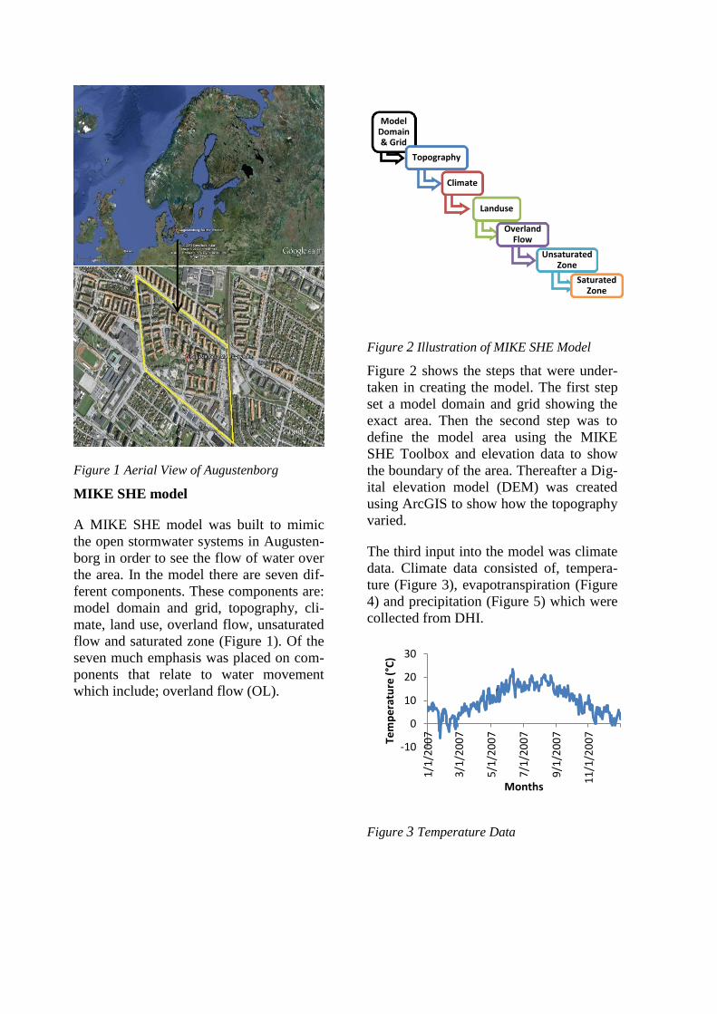
Figure 1 Aerial View of Augustenborg

MIKE SHE model

A MIKE SHE model was built to mimic

the open stormwater systems in Augusten-

borg in order to see the flow of water over

the area. In the model there are seven dif-

ferent components. These components are:

model domain and grid, topography, cli-

mate, land use, overland flow, unsaturated

flow and saturated zone (Figure 1). Of the

seven much emphasis was placed on com-

ponents that relate to water movement

which include; overland flow (OL).

Figure 2 Illustration of MIKE SHE Model

Figure 2 shows the steps that were under-

taken in creating the model. The first step

set a model domain and grid showing the

exact area. Then the second step was to

define the model area using the MIKE

SHE Toolbox and elevation data to show

the boundary of the area. Thereafter a Dig-

ital elevation model (DEM) was created

using ArcGIS to show how the topography

varied.

The third input into the model was climate

data. Climate data consisted of, tempera-

ture (Figure 3), evapotranspiration (Figure

4) and precipitation (Figure 5) which were

collected from DHI.

Figure 3 Temperature Data

Model Domain & Grid

Topography

Climate

Landuse

Overland Flow

Unsaturated Zone

Saturated Zone

-10

0

10

20

30

1/1

/20

07

3/1

/20

07

5/1

/20

07

7/1

/20

07

9/1

/20

07

11

/1/2

00

7

Tem

pe

ratu

re (

°C)

Months

Figure 4 Evapotranspiration data

Figure 5 Rainfall Data

The fourth step is to describe land use by

illustrating the open ditches and swales.

The green roofs were ignored because their

impact during extreme rainfall conditions

would be minimal. In the MIKE SHE

model, vegetation properties were set same

over the whole area. Vegetation properties

were used to calculate the actual evapo-

transpiration from crop reference evapo-

transpiration (DHI, 2012). The key vegeta-

tion properties designed in the model were

are Leaf Area Index (LAI) and Root Depth

(RD), (Yan, o.a., 2012). Generally the LAI

and RD can be specified directly as a time

series. Otherwise, they could be defined as

a crop cycle in the vegetation properties

editor.

The fifth component that was described in

the model was overland flow. The finite

difference method was selected to simulate

overland flow. There were several items

required for calculation processes in the

main dialogue of the model for overland

flow. There items include:

1. Manning number; was equivalent to the

Stickler roughness coefficient

2. Detention Storage; was used to limit the

amount of water that can flow over the

ground surface

3. Initial Water Depth on the ground sur-

face; was used for the overland flow calcu-

lations and the initial water depth is usual-

ly set to 0

4. Surface-Sub surface leakage coefficient;

the value of the leakage coefficient was set

to zero for all buildings as water cannot

infiltrate through the buildings and the rest

of the area was set to have full contact to

the UZ/SZ zones.

The sixth step in the design of the model

was defining the unsaturated zone. In

MIKE SHE there are three methods that

can be used to calculate unsaturated flow.

These methods include Richards’s equa-

tion, the gravity flow and the two-layer

water balance. In this instance Richards

equation was used which was specified in

the simulation specification dialog. Rich-

ards equation is quoted by (DHI, 2012) as

the, “driving force for transport of water in

the unsaturated zone is the gradient of the

hydraulic head, h, which includes a gravi-

tational component, z, and a pressure com-

ponent, ψ.” Its equation is:

( ) (

)

Where,

K; is the hydraulic conductivity

ψ is the pressure head

z; is the elevation

0

20

40

60

80

100

120

140

1 3 5 7 9 11

Po

ten

tial

Eva

po

tran

spir

atio

n

(mm

/mo

nth

)

Months of the year

0

50

100

150

200

250

Rai

nfa

ll (m

m/m

on

th)

Year

Jan

Feb

Mar

Apr

May

Jun

θ; is the water content

t; is timed

Soil profile definitions were defined using

Tables 1-4, listed below:

Soil profile definition

Table 1 Soil Profile

From

depth

To

depth

Soil type

1 0m 0.3m Matjord 0

2 0.3m 2m Coarse Till (0-0.5m)

3 2m 5m Coarse Till (0.5-2m)

Note: The Matjord was inserted as a top

layer of soil.

Table 2 Geological layers

Soil layers

Lower

level

Kh Kv Specific

Yield

Storage

Matjord -0.3 1e-

006

1e-

006

0.2 0.0001

Course

Till 0-0.5

-2 2e-

005

5e-

006

0.2 0.0001

Course

Till 0.5-2

-5 1e-

006

1e-

007

0.2 0.0001

Table 3 Swale definitions

From

depth

To depth Soil type

1 0m 0.3m Matjord 0

2 0.3m 2m Gravel

3 2m 5m Coarse Till (0.5-2m)

The seventh step in design of the model

was the saturated zone. The creation of the

saturated zone in the MIKE SHE is based

on 3D Finite Difference Method which

involves defining the geological model,

vertical numerical discretisation, initial

conditions and boundary conditions.

The MIKE SHE graphical user interface

shows that the initial conditions are de-

fined as a property of numerical layer

whereas the geological models and the

vertical discretisation are independent.

Drainage

Drainage in the MIKE model was set

based on permeability. Most areas in the

study area are permeable due to the open

stormwater solutions. The areas that are

not permeable are concrete ditches, park-

ing places and buildings. In MIKE SHE,

the areas where buildings are located were

set to -1.7 m (an estimated figure indicat-

ing no infiltration in the top soil; matjord

& upper course till layers) relative to the

ground taking into account the geological

layering of soil. Other areas where set to

zero indicating that water would be able to

infiltrate into those areas.

Computational layers

Of the three geological layers two compu-

tational layers were formed. The first two

layers (Matjord and Course Till 0-0.5)

were combined into one layer and the bot-

tom layer (Course Till 0.5-2) was left as a

layer on its own (Table 4).

Table 4Computational layers

Computational

Layers

Lower

level

Initial Potential

Head

L1 -2 -1.5

L2 -5 -1.5

Calibration data

In this study there was no observed data

which meant that there was no calibration

and validation to compare the results of the

model.

Description of open stormwater solu-

tions in MIKE SHE model

In this study some of the open solutions

including storage ponds, swales and open

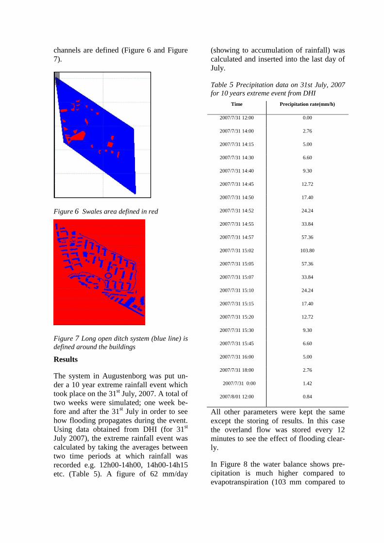
channels are defined (Figure 6 and Figure

7).

Figure 6 Swales area defined in red

Figure 7 Long open ditch system (blue line) is

defined around the buildings

Results

The system in Augustenborg was put un-

der a 10 year extreme rainfall event which

took place on the 31st July, 2007. A total of

two weeks were simulated; one week be-

fore and after the 31st July in order to see

how flooding propagates during the event.

Using data obtained from DHI (for 31st

July 2007), the extreme rainfall event was

calculated by taking the averages between

two time periods at which rainfall was

recorded e.g. 12h00-14h00, 14h00-14h15

etc. (Table 5). A figure of 62 mm/day

(showing to accumulation of rainfall) was

calculated and inserted into the last day of

July.

Table 5 Precipitation data on 31st July, 2007

for 10 years extreme event from DHI

Time Precipitation rate(mm/h)

2007/7/31 12:00 0.00

2007/7/31 14:00 2.76

2007/7/31 14:15 5.00

2007/7/31 14:30 6.60

2007/7/31 14:40 9.30

2007/7/31 14:45 12.72

2007/7/31 14:50 17.40

2007/7/31 14:52 24.24

2007/7/31 14:55 33.84

2007/7/31 14:57 57.36

2007/7/31 15:02 103.80

2007/7/31 15:05 57.36

2007/7/31 15:07 33.84

2007/7/31 15:10 24.24

2007/7/31 15:15 17.40

2007/7/31 15:20 12.72

2007/7/31 15:30 9.30

2007/7/31 15:45 6.60

2007/7/31 16:00 5.00

2007/7/31 18:00 2.76

2007/7/31 0:00 1.42

2007/8/01 12:00 0.84

All other parameters were kept the same

except the storing of results. In this case

the overland flow was stored every 12

minutes to see the effect of flooding clear-

ly.

In Figure 8 the water balance shows pre-

cipitation is much higher compared to

evapotranspiration (103 mm compared to

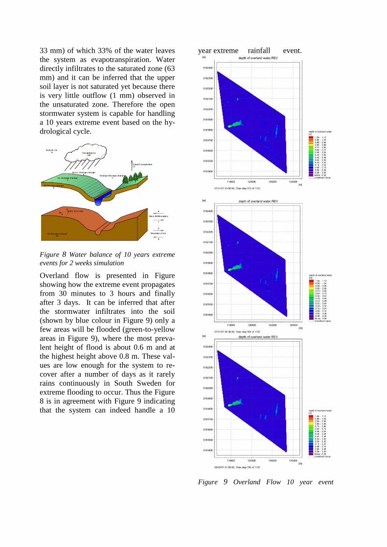
33 mm) of which 33% of the water leaves

the system as evapotranspiration. Water

directly infiltrates to the saturated zone (63

mm) and it can be inferred that the upper

soil layer is not saturated yet because there

is very little outflow (1 mm) observed in

the unsaturated zone. Therefore the open

stormwater system is capable for handling

a 10 years extreme event based on the hy-

drological cycle.

Figure 8 Water balance of 10 years extreme

events for 2 weeks simulation

Overland flow is presented in Figure

showing how the extreme event propagates

from 30 minutes to 3 hours and finally

after 3 days. It can be inferred that after

the stormwater infiltrates into the soil

(shown by blue colour in Figure 9) only a

few areas will be flooded (green-to-yellow

areas in Figure 9), where the most preva-

lent height of flood is about 0.6 m and at

the highest height above 0.8 m. These val-

ues are low enough for the system to re-

cover after a number of days as it rarely

rains continuously in South Sweden for

extreme flooding to occur. Thus the Figure

8 is in agreement with Figure 9 indicating

that the system can indeed handle a 10

year extreme rainfall event.

Figure 9 Overland Flow 10 year event

Similarly in the 100 year extreme event the

process was simulated using the same pro-

cedure as the 10 year event. Also, the same

procedure was used (as in the 10 year

event) to calculate the extreme precipita-

tion value that was inserted on the last day

of July (Table 6). An amount of 128

mm/day was obtained according to accu-

mulation of rainfall for each time period

where it rained.

Table 6 Precipitation data on 31st July, 2007

for 100 years extreme event from DHI

Time Precipitation rate(mm/h)

2007/7/31 12:00 0.00

2007/7/31 14:00 4.47

2007/7/31 14:15 8.64

2007/7/31 14:30 11.88

2007/7/31 14:40 17.64

2007/7/31 14:45 25.20

2007/7/31 14:50 36.36

2007/7/31 14:52 53.28

2007/7/31 14:55 77.76

2007/7/31 14:57 136.80

2007/7/31 15:02 205.92

2007/7/31 15:05 136.80

2007/7/31 15:07 77.76

2007/7/31 15:10 53.28

2007/7/31 15:15 36.36

2007/7/31 15:20 25.20

2007/7/31 15:30 17.64

2007/7/31 15:45 11.88

2007/7/31 16:00 8.64

2007/7/31 18:00 4.47

2007/7/31 0:00 2.15

2007/8/01 12:00 1.22

From the water balance (Figure 10), pre-

cipitation is much higher compared to 10

years extreme event (169 mm compared to

103 mm), of which 119 mm of water infil-

trates to the saturated zone while 33 mm

evaporated. The evapotranspiration is still

33 mm which is the same as in the 10 year

extreme event simulation results because

no change was made to the vegetation or

soil layers. However, 5 mm of water at the

boundary flow was observed in unsaturat-

ed zone compared to no flow of water out

of the boundary in the UZ in the 10 year

extreme event simulation. This could

mean that in the 100 year event some areas

within the area would be at risk of flooding

as there is complete saturation in the un-

saturated and saturated zones causing out-

flow of water at the boundary.

By checking of the overland flow depth in

(Figure 11), most of the area where swales

are located flooded with an average depth

of water of about 0.8 m with a few areas

above 1.4 m. Some residential areas are

also under risking flooding, which puts the

system under stress in handling the 100

years extreme rainfall because most of soil

is saturated.

Figure 10 Water balance of 100 years extreme

events for 2 weeks simulation

Figure 11 Overland Flow 100 year event

Discussion

The results showed that the system was

capable of handling a 10 year event over a

period of 12 hours. Generally over the en-

tire area the depth of overland flow was in

the range of 0.15 m with only the region

were swale are located above 0.6 m indi-

cating that rather small amounts of water

flowing. It can be inferred that most of the

water infiltrated into the system and there

was no flow of water through the boundary

and flooding in the residential area.

The 100 year period yielded different re-

sults and for the first time the unsaturated

zone reached its threshold and there was

overland flow on the ground surface.

There were a number of areas of with val-

ues above 1m which indicated that there is

severe a risk of flooding during this ex-

treme event. Also 5mm of outflow was

recorded on the water balance indicating

water flowing out of the system. This is an

indication that in the unlikely event of an

extreme rain for more than 24 hours, there

will definitely be an accumulation of water

that will cause a high risk of flooding.

In addition, with global trends including

climate change it can be said that this

event puts the system under a lot of pres-

sure to handle so much water. Thus, it can

be concluded that during this scenario the

system is under a dangerous risk of flood-

ing and there needs to some measures put

in place to ensure that if large amount of

rainfall falls like in this scenario it will be

able to handle it. On the contrary, it is also

rare that a 100 year extreme event can oc-

cur in the South of Sweden but we should

not neglect anything hence the investiga-

tion.

Most of the open stormwater solutions

performed their specific function with a

few exceptions. It can be seen the areas

where ponds are located, there is no flood-

ing meaning that they worked as a storage

medium even in the model which is their

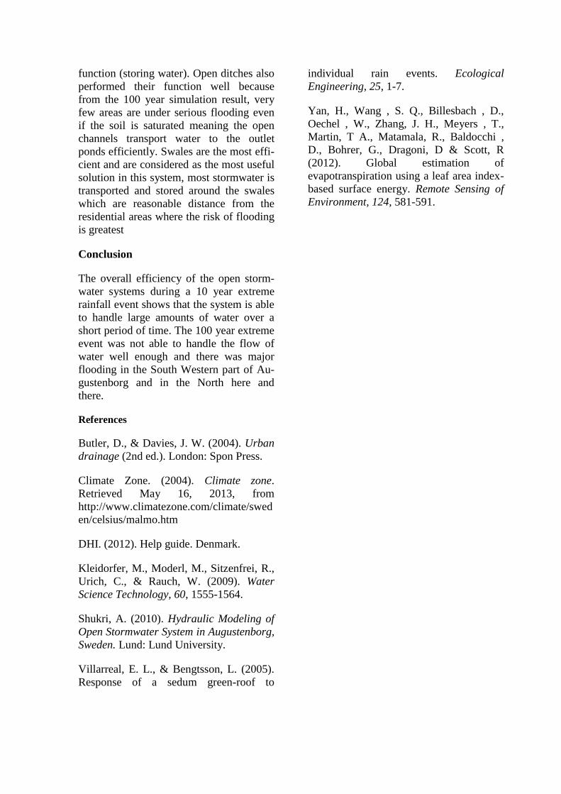
function (storing water). Open ditches also

performed their function well because

from the 100 year simulation result, very

few areas are under serious flooding even

if the soil is saturated meaning the open

channels transport water to the outlet

ponds efficiently. Swales are the most effi-

cient and are considered as the most useful

solution in this system, most stormwater is

transported and stored around the swales

which are reasonable distance from the

residential areas where the risk of flooding

is greatest

Conclusion

The overall efficiency of the open storm-

water systems during a 10 year extreme

rainfall event shows that the system is able

to handle large amounts of water over a

short period of time. The 100 year extreme

event was not able to handle the flow of

water well enough and there was major

flooding in the South Western part of Au-

gustenborg and in the North here and

there.

References

Butler, D., & Davies, J. W. (2004). Urban

drainage (2nd ed.). London: Spon Press.

Climate Zone. (2004). Climate zone.

Retrieved May 16, 2013, from

http://www.climatezone.com/climate/swed

en/celsius/malmo.htm

DHI. (2012). Help guide. Denmark.

Kleidorfer, M., Moderl, M., Sitzenfrei, R.,

Urich, C., & Rauch, W. (2009). Water

Science Technology, 60, 1555-1564.

Shukri, A. (2010). Hydraulic Modeling of

Open Stormwater System in Augustenborg,

Sweden. Lund: Lund University.

Villarreal, E. L., & Bengtsson, L. (2005).

Response of a sedum green-roof to

individual rain events. Ecological

Engineering, 25, 1-7.

Yan, H., Wang , S. Q., Billesbach , D.,

Oechel , W., Zhang, J. H., Meyers , T.,

Martin, T A., Matamala, R., Baldocchi ,

D., Bohrer, G., Dragoni, D & Scott, R

(2012). Global estimation of

evapotranspiration using a leaf area index-

based surface energy. Remote Sensing of

Environment, 124, 581-591.