X-FEM for FSI Interfaces - CIMNEcongress.cimne.com/cfsi/frontal/doc/ppt/14.pdf · 1 / 40 X-FEM for...

1 / 40

X-FEM for FSI Interfaces

Andreas Kolke

Institute for Structural AnalysisTechnische Universitat Braunschweig

03 May 2006

Advanced Computational Methods

for Fluid-Structure Interaction

Aim of the Talk

Aim of the TalkConceptional Use ofX-FEM for FSIProblems

Interaction of Fluidand Structure

CharacteristicSolutions

Approximation ofSpecial Solutions

X-FEM (I):Introduction

X-FEM (II):Evolving Solutions

X-FEM (III):Enriching the Flow

X-FEM (IV):Coupling Conditions

MappingConfigurations

X-FEM for FSI:Applications

2 / 40

Conceptional Use of X-FEM for FSI Problems

Aim of the TalkConceptional Use ofX-FEM for FSIProblems










3 / 40

Physics:

Modeling coupled problems Fluid-structure interaction: special solutions? A priori knowledge of solution characteristics in FSI?

Numerics:

Strategies of discretization X-FEM X-FEM for FSI (space-time finite element method)

Interaction of Fluid and Structure

Aim of the Talk

Interaction of Fluidand StructureOscillators &Mechanisms ofExcitation

Examples

Coupled Problem









4 / 40

Oscillators & Mechanisms of Excitation

Aim of the Talk


Examples

Coupled Problem









5 / 40

Oscillators:

Body oscillatorsstructures of discrete/distributed mass/elasticity

Fluid oscillatorsfluids of discrete/distributed mass/compressibility

Mechanisms of Excitation:

Extraneously induced excitationvariations in the flow field (turbulence, noise)

Instability-induced excitationvariations due to flow-intrinsic instability(vortex shedding, shear layers, sensitive interfaces)

Movement-induced excitationvariations due to changes of geometry(flutter, galloping, slender structures in axial flow, ...)

Examples

Aim of the Talk


Examples

Coupled Problem









6 / 40

Coupled Problem

Aim of the Talk


Examples

Coupled Problem









7 / 40

Multiple bodies in interaction via boundary or domain.

s

nΩ2Ω1

Γ2

Γ1

Σ

Figure 1: boundary-coupled two-field system.

Model equations for fluid & structure,Boundary and initial conditions,Model equations for coupling at common interface.

Characteristic Solutions

Aim of the Talk


CharacteristicSolutionsSpecial SolutionProperties with FSI

General Approach

Thin Structures

Tips and Edges

Wall Effects

Bluff Bodies








8 / 40

Special Solution Properties with FSI

Aim of the Talk



General Approach

Thin Structures

Tips and Edges

Wall Effects

Bluff Bodies








9 / 40

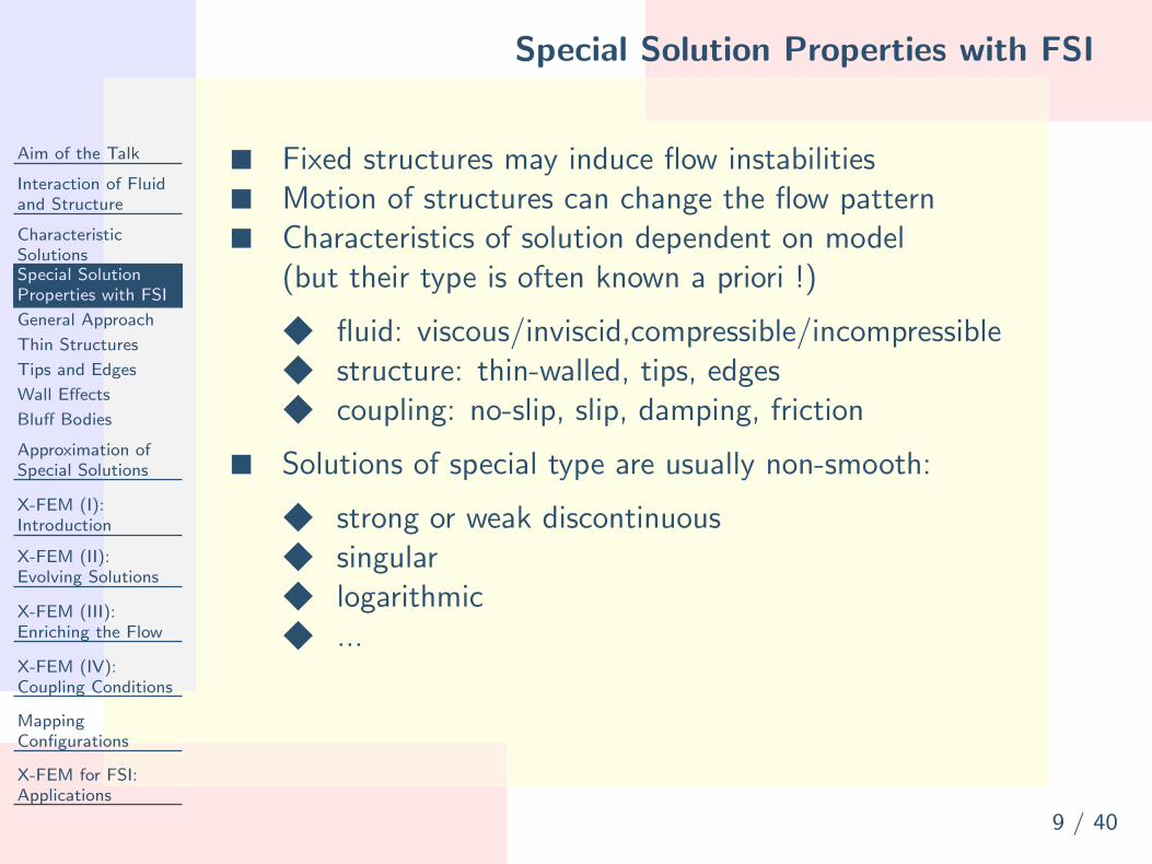
Fixed structures may induce flow instabilities Motion of structures can change the flow pattern Characteristics of solution dependent on model

(but their type is often known a priori !)

fluid: viscous/inviscid,compressible/incompressible structure: thin-walled, tips, edges coupling: no-slip, slip, damping, friction

Solutions of special type are usually non-smooth:

strong or weak discontinuous singular logarithmic ...

General Approach

Aim of the Talk



General Approach

Thin Structures

Tips and Edges

Wall Effects

Bluff Bodies








10 / 40

Demand: develop & apply simple models to use as afirst approximation to a complex FSI process

Action: accept resulting type of expectable solution

Advantage: avoid time-consuming resolution of fullmodel’s length and time scales

Disadvantage: need for sophisticated solutiontechnique to capture solution properties

Thin Structures

Aim of the Talk



General Approach

Thin Structures

Tips and Edges

Wall Effects

Bluff Bodies








11 / 40

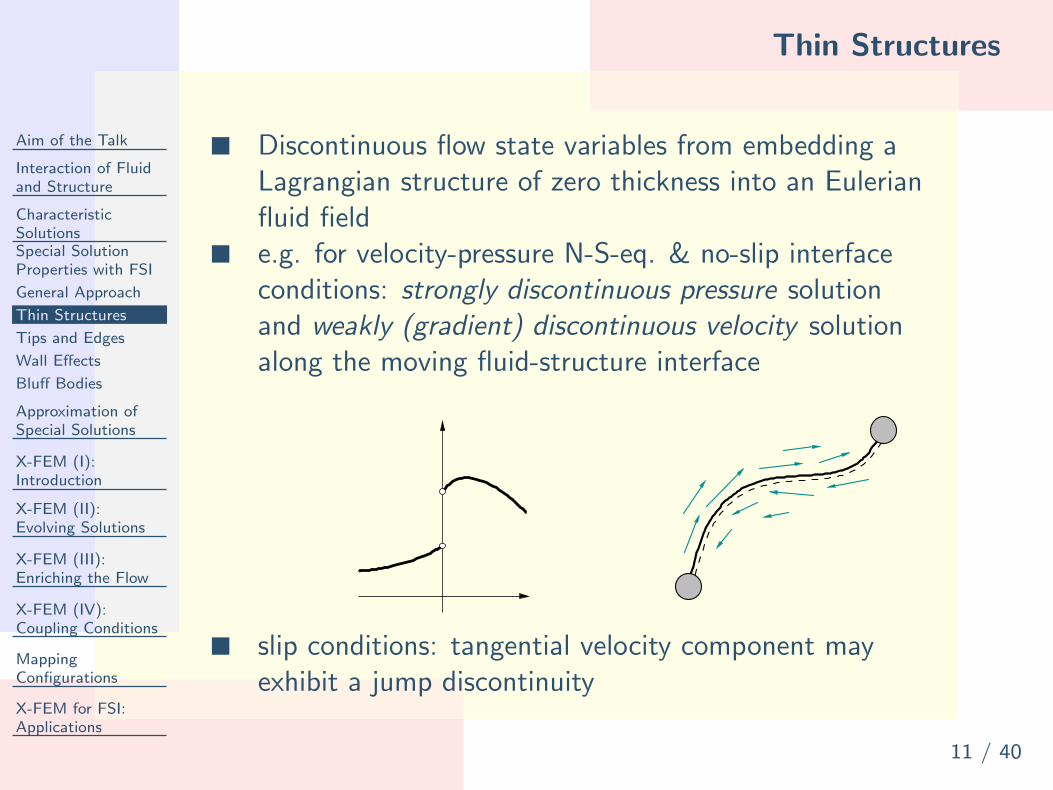
Discontinuous flow state variables from embedding aLagrangian structure of zero thickness into an Eulerianfluid field

e.g. for velocity-pressure N-S-eq. & no-slip interfaceconditions: strongly discontinuous pressure solutionand weakly (gradient) discontinuous velocity solutionalong the moving fluid-structure interface

slip conditions: tangential velocity component mayexhibit a jump discontinuity

Tips and Edges

Aim of the Talk



General Approach

Thin Structures

Tips and Edges

Wall Effects

Bluff Bodies








12 / 40

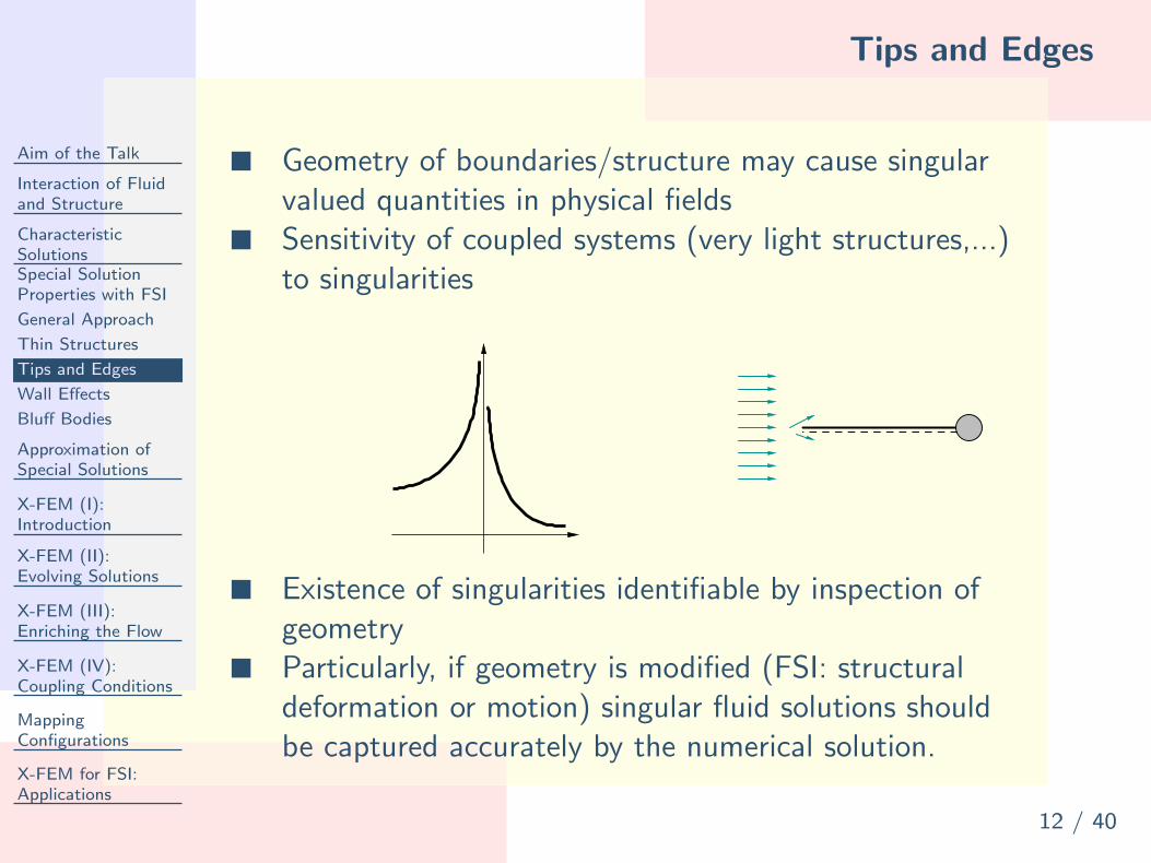
Geometry of boundaries/structure may cause singularvalued quantities in physical fields

Sensitivity of coupled systems (very light structures,...)to singularities

Existence of singularities identifiable by inspection ofgeometry

Particularly, if geometry is modified (FSI: structuraldeformation or motion) singular fluid solutions shouldbe captured accurately by the numerical solution.

Wall Effects

Aim of the Talk



General Approach

Thin Structures

Tips and Edges

Wall Effects

Bluff Bodies








13 / 40

Representation of (turbulent) boundary layer Wall functions

Reduce computational costs by using the a prioriknowledge of logarithmic type of the solution

Location of the boundary layer is defined by theinterface position

Bluff Bodies

Aim of the Talk



General Approach

Thin Structures

Tips and Edges

Wall Effects

Bluff Bodies








14 / 40

Representation of impinging shear layers, sheddingvortices or interface instabilities caused by bluff bodiesor fixed/moving boundaries

location of special solutions in the vicinity of interfacesare easiliy allocable

Approximation of Special Solutions

Aim of the Talk




DomainDiscretization

Adaptivity

Choosing the Basis







15 / 40

Domain Discretization

Aim of the Talk





Adaptivity

Choosing the Basis







16 / 40

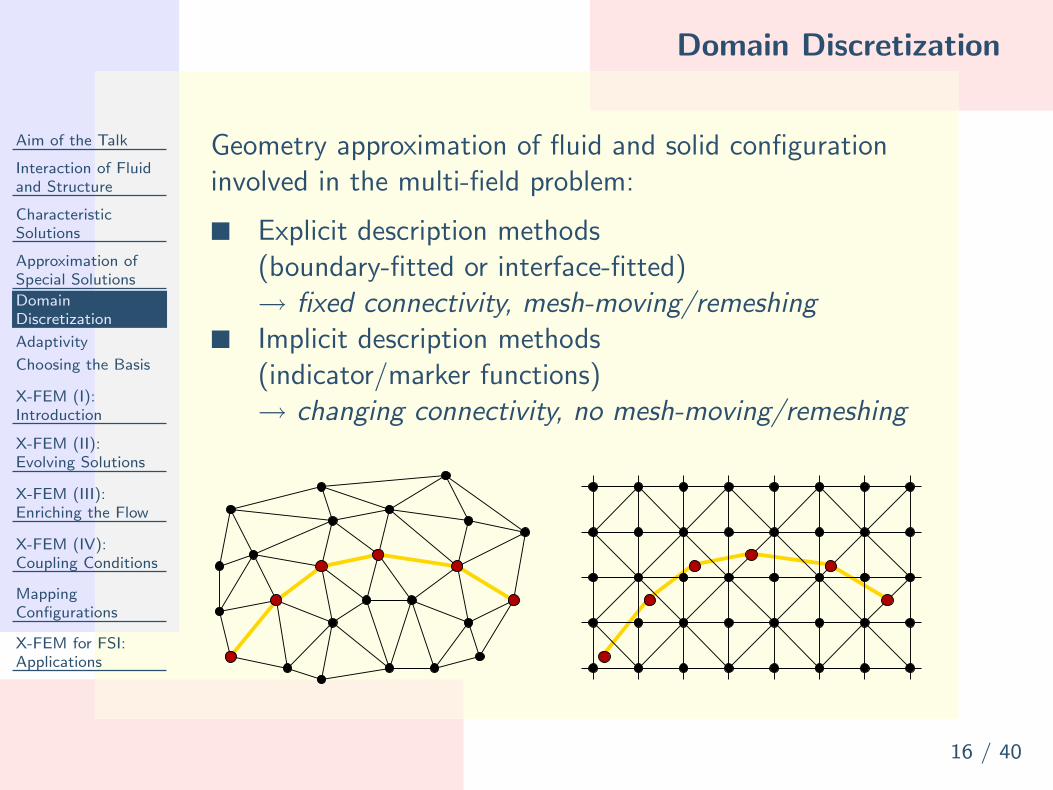
Geometry approximation of fluid and solid configurationinvolved in the multi-field problem:

Explicit description methods(boundary-fitted or interface-fitted)→ fixed connectivity, mesh-moving/remeshing

Implicit description methods(indicator/marker functions)→ changing connectivity, no mesh-moving/remeshing

Adaptivity

Aim of the Talk





Adaptivity

Choosing the Basis







17 / 40

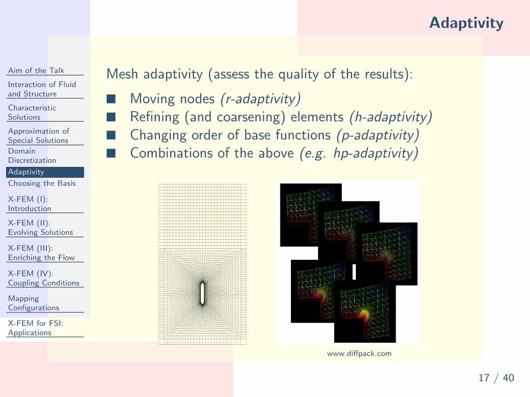
Mesh adaptivity (assess the quality of the results):

Moving nodes (r-adaptivity) Refining (and coarsening) elements (h-adaptivity) Changing order of base functions (p-adaptivity) Combinations of the above (e.g. hp-adaptivity)

www.diffpack.com

Choosing the Basis

Aim of the Talk





Adaptivity

Choosing the Basis







18 / 40

Choosing the basis of approximation:

Higher degree piecewise polynomial basis functions(spectral element methods)

Rational basis functions Extrinsic enriched approximation using the

Partition of Unity Method (PUM) → PU-FEM, X-FEM

Appropriate modification of the ansatz to the approximation so that

the function space of the modified approximation is made able to

reflect the essential properties of the solution to the model equations.

X-FEM (I): Introduction

Aim of the Talk





Partition of Unity I

Partition of Unity II

Extrinsic Enrichmentof FE Approximation






19 / 40


Aim of the Talk













20 / 40

A set of functions Nk is called a partition of unity (PU) if

X

k

Nk(x)p(xk) = p(x) ∀ x ∈ Ω, (1)

where p is a polynomial basis of order n.

Within a weighted residual formulation these functions are able torepresent any analytical solution of polynomial type up to order nexactly.

Partition of unity methods 1 2 enrich the approximation space by anadditional basis g and choose an ansatz of the form

uhPU (x) =

X

k

Nk(x)g · uk (2)

with modified properties of approximation.

1I. Babuska and J. M. Melenk. The Partition of Unity Method. IJNME, 40:727–758, 1997.

2J. M. Melenk and I. Babuska. The Partition of Unity Finite Element Method: Basic Theory and

Applications. CMAME, 39:289–314, 1996.


Aim of the Talk













21 / 40

The basis g may incorporate

Lagrange or Taylor polynomials, Discontinuous functions (Heaviside, Dirac delta, absolute value), Singular functions, Transcendental functions (trigonometric, logarithmic)

or other appropriate expressions.

Any available a priori known information on thecharacteristic properties of the expected solution tothe modeled problem should be taken into accountwhile composing the enriched basis g.

Extrinsic Enrichment of FE Approximation

Aim of the Talk













22 / 40

The partition of unity ansatz can be expressed by an extrinsicenrichment using

g =

»

1ψ

–

and uk =

»

uk

u∗k

–

(3)

to extend the standard approximation (of ansatz functions Nk) by theproducts Nkψ.

The enrichment function ψ modifies the standard approximation andcreates an extended approximation

uhext(x) =

X

k∈N std

Nk(x) uk +X

j∈N ext

Nj(x)ψ(x) u∗j (4)

with additional coefficients u∗j .

X-FEM (II): Evolving Solutions

Aim of the Talk






EvolvingNon-smoothSolutionsSpace-Time FiniteElement MethodExtrinsic Enrichmentof Space-Time FEM





23 / 40

Evolving Non-smooth Solutions

Aim of the Talk











24 / 40

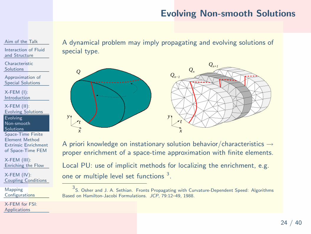
A dynamical problem may imply propagating and evolving solutions ofspecial type.

y

x

t

Q

y

QQ

Qn

n−1

n+1

x

t

A priori knowledge on instationary solution behavior/characteristics →proper enrichment of a space-time approximation with finite elements.

Local PU: use of implicit methods for localizing the enrichment, e.g.

one or multiple level set functions 3.

3S. Osher and J. A. Sethian. Fronts Propagating with Curvature-Dependent Speed: Algorithms

Based on Hamilton-Jacobi Formulations. JCP, 79:12–49, 1988.

Space-Time Finite Element Method

Aim of the Talk











25 / 40

Methodically uniform discretization of space and time applyingthe finite element approach (Oden, Argyris and Fried)

y

x

t

Q

y

QQ

Qn

n−1

n+1

x

t

Straightforward applicability of X-FEM technology to describeevolving non-smooth solutions within the space-time domain

Enriched space-time finite elements enables to capturestrong/gradient discontinuities, singularities, boundary layerspropagating through the domain

Approximation in space-time with the unknown coefficients uk:

uhstd(x, t) =

X

k∈N std

Nk(x, t) uk (5)

Extrinsic Enrichment of Space-Time FEM

Aim of the Talk











26 / 40

Combination of level set method, local partition of unityenrichment & space-time finite element discretization for evolvingsolution features – discontinuities at thin-walled structures 4 5

Extended approximation in space-time with coefficients uk andadditional unknowns u∗

j of the enrichment:

uhext(x, t) =

X

k∈N std

Nk(x, t) uk +X

j∈N ext

Nj(x, t)ψj(x, t) u∗j (6)

The nodally defined enrichment function

ψj(x, t) = ψ(x, t) − ψ(xj , tj) (7)

incorporates placement of local enrichment within the space-time

finite element and ensures Kronecker-δ property of the approximation.

4A. Legay and A. Kolke. A locally enriched space-time finite element method for fluid-structure

interaction – Part I: Prescribed structural motion. in preparation5A. Kolke and A. Legay. A locally enriched space-time finite element method for fluid-structure

interaction – Part II: Thin flexible structures. in preparation

X-FEM (III): Enriching the Flow

Aim of the Talk







Thin Structures:Discontinuities




27 / 40

Thin Structures: Discontinuities

Aim of the Talk







Thin Structures:Discontinuities




28 / 40

Strong and weak discontinuities in a velocity-pressure fluidformulation realized by jump-type enrichment function ψj(x, t)

Locally enriched velocity/pressure approximation:

vhext(x, t) =

X

k∈N std

Nk(x, t) vk +X

j∈N ext

Nj(x, t)ψj(x, t) v∗j

phext(x, t) =

X

k∈N std

Nk(x, t) pk +X

j∈N ext

Nj(x, t)ψj(x, t) p∗j (8)

with additional unknowns v∗j and p∗j .

Continuity of the velocity field (no-slip) at the fluid-structureinterface to be ensured by an appropriate method.

Enrichment function determined by evaluation of the level setfunction φ

ψj(x, t) =1

2(1 − sign φ(x, t) · sign φ(xj , tj)) (9)

at the nodes j and at the point within the domain.

X-FEM (IV): Coupling Conditions

Aim of the Talk








Penalty Methods

Lagrange MultiplierMethodsDistributed LMMethod



29 / 40

Penalty Methods

Aim of the Talk








Penalty Methods




30 / 40

Add a penalty term of constraint to the weak form

α

∫

R

δw(u+− u

−)dR (10)

Factor α >> 1 Constraint accuracy increases with large numbers of α

Advantage: size of system of equations is constant Disadvantage: influences condition number of resulting

system of equations, ill-conditioning

Nitsche’s method(consistent improvement of the penalty method):several problem dependent penalty terms with α-valuesconsiderably smaller

Lagrange Multiplier Methods

Aim of the Talk








Penalty Methods




31 / 40

Add a Lagrange multiplier formulation of constraint tothe weak form∫

R

δλ(u+− u

−)dR −

∫

R

δ(u+− u

−)λdR (11)

Advantage: General and accurate approach Disadvantage: LM need to be solved additionally to

discrete field variables, set of interpolation functionsfor LM required

Discretization of λ for ’evolving’ constraints?(FSI problems on fixed meshes, ...)

Distributed LM Method

Aim of the Talk








Penalty Methods




32 / 40

Since the fluid-structure interface is moving and deforming thediscrete description of interface tractions in an explicit manner isnot easy to realize.

Apply an implicit technique (level set approach) as it is realizedfor interface representation.

u1

u2

φ = 0

tt

LM λ(x, t) represented by zero level set φ(x, t) = 0 ofhigher-dimensional function λ(x, t)

λ(x, t) = λ(x, t) δD(φ(x, t)) , (12)

where δD is the Dirac delta function.

Implicit formulation of the Lagrangian multiplier!

Mapping Configurations

Aim of the Talk









Level SetRepresentation ofThin-walledStructures


33 / 40

Level Set Representation of Thin-walled Structures

Aim of the Talk









Level SetRepresentation ofThin-walledStructures


34 / 40

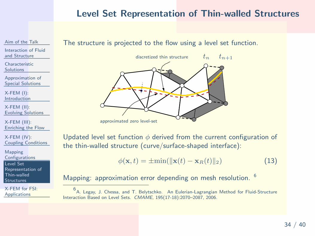
The structure is projected to the flow using a level set function.

approximated zero level-set

discretized thin structure tn tn+1

Updated level set function φ derived from the current configuration ofthe thin-walled structure (curve/surface-shaped interface):

φ(x, t) = ±min(‖x(t) − xR(t)‖2) (13)

Mapping: approximation error depending on mesh resolution. 6

6A. Legay, J. Chessa, and T. Belytschko. An Eulerian-Lagrangian Method for Fluid-Structure

Interaction Based on Level Sets. CMAME, 195(17-18):2070–2087, 2006.

X-FEM for FSI: Applications

Aim of the Talk










Piston I

Piston II

Piston III

Supported Beam

Rotating Beam

35 / 40

Piston I

Aim of the Talk










Piston I

Piston II

Piston III

Supported Beam

Rotating Beam

36 / 40

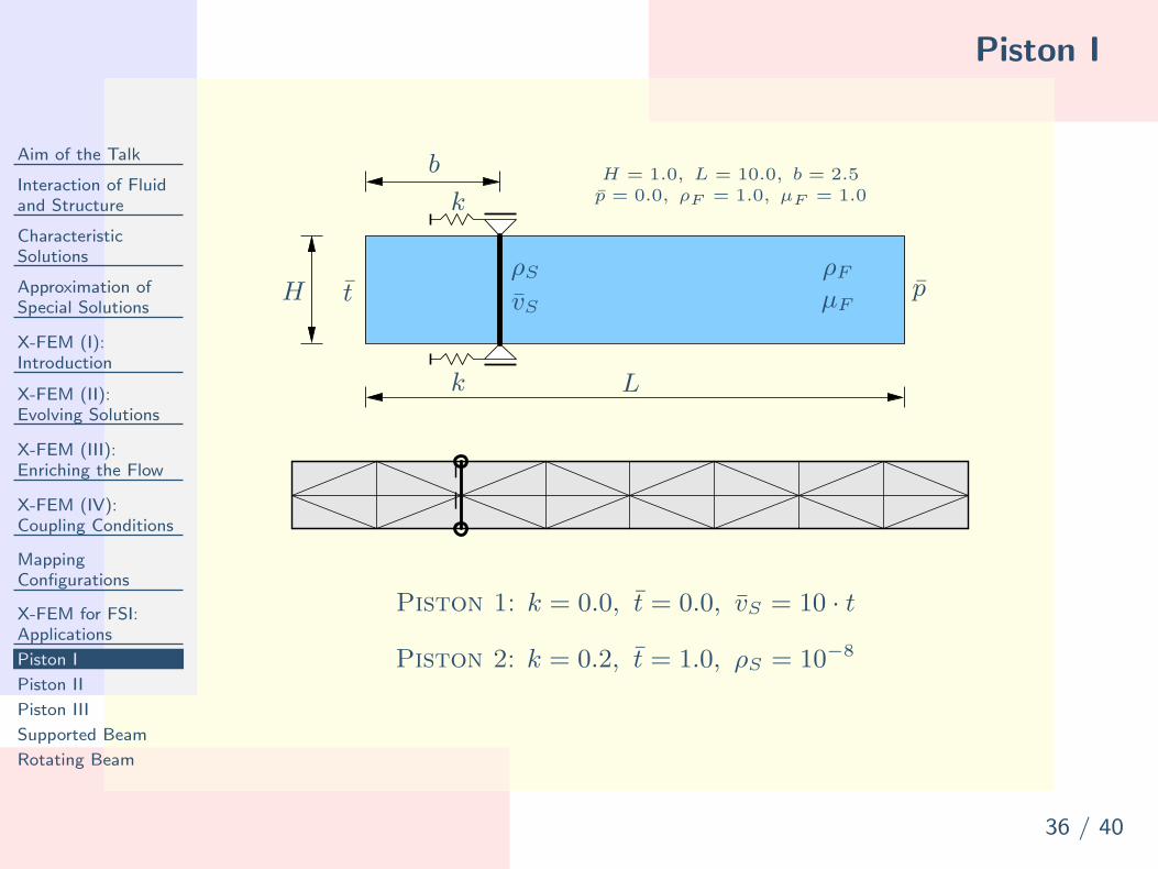
L

H

b

k

k

ρF

µF

ρS

vSt p

H = 1.0, L = 10.0, b = 2.5

p = 0.0, ρF = 1.0, µF = 1.0

Piston 1: k = 0.0, t = 0.0, vS = 10 · t

Piston 2: k = 0.2, t = 1.0, ρS = 10−8

Piston II

Aim of the Talk










Piston I

Piston II

Piston III

Supported Beam

Rotating Beam

37 / 40

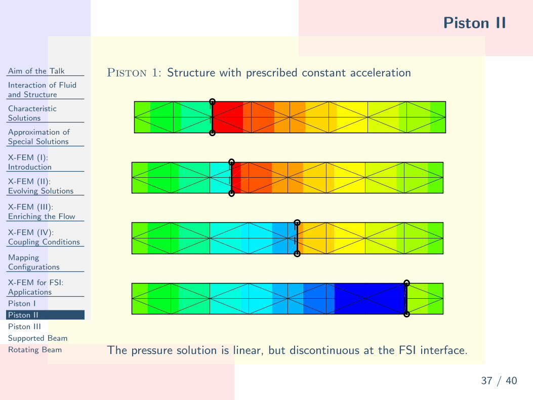
Piston 1: Structure with prescribed constant acceleration

The pressure solution is linear, but discontinuous at the FSI interface.

Piston III

Aim of the Talk










Piston I

Piston II

Piston III

Supported Beam

Rotating Beam

38 / 40

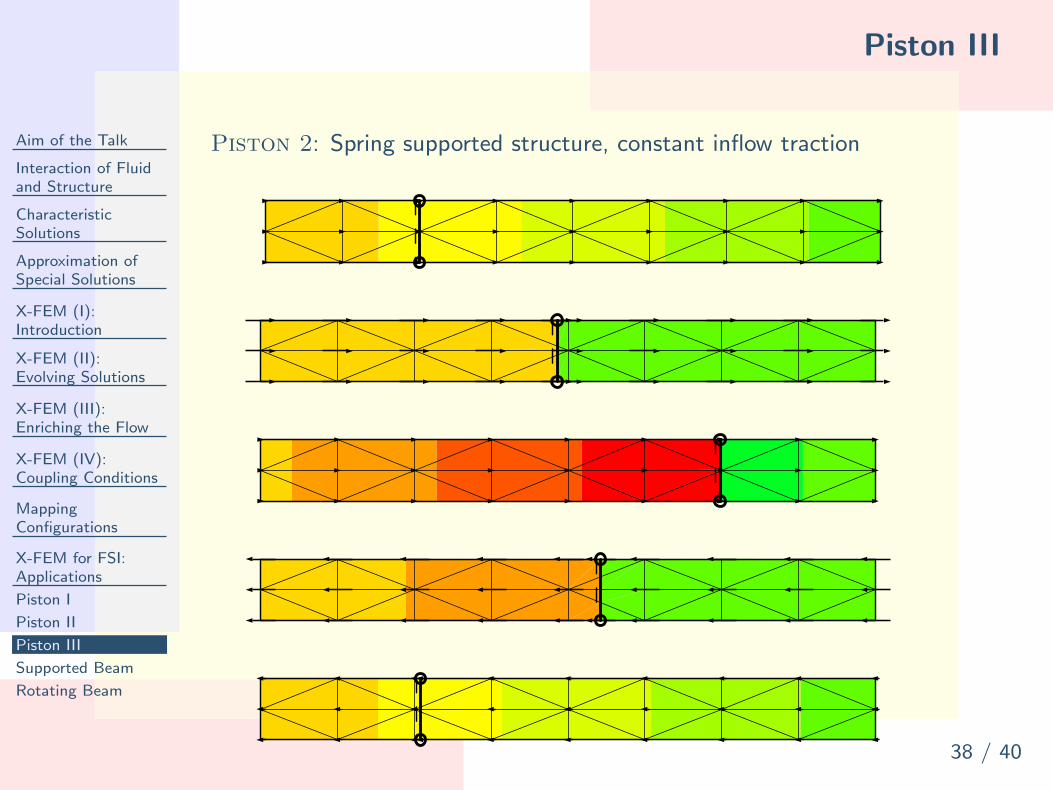
Piston 2: Spring supported structure, constant inflow traction

Supported Beam

Aim of the Talk










Piston I

Piston II

Piston III

Supported Beam

Rotating Beam

39 / 40movie

Rotating Beam

Aim of the Talk










Piston I

Piston II

Piston III

Supported Beam

Rotating Beam

40 / 40

movie: pressure field movie: level set function

X-FEM for FSI Interfaces - CIMNEcongress.cimne.com/cfsi/frontal/doc/ppt/14.pdf · 1 / 40 X-FEM for...

Documents

Transcript of X-FEM for FSI Interfaces - CIMNEcongress.cimne.com/cfsi/frontal/doc/ppt/14.pdf · 1 / 40 X-FEM for...