Wynda Astutik

IPR Modeling for Coning Wells

Thesis for the degree of Master of Science

TrondheimAugust 12, 2012

Norwegian University of Science and TechnologyFaculty of Engineering Science and TechnologyDepartment of Petroleum Engineering and Applied Geophysics

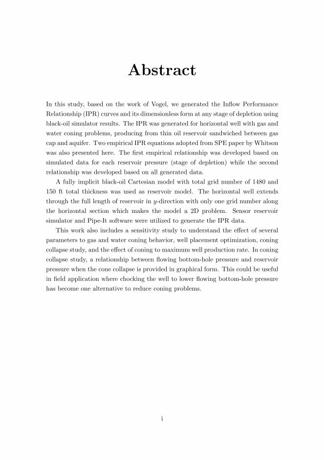
Abstract

In this study, based on the work of Vogel, we generated the Inflow Performance

Relationship (IPR) curves and its dimensionless form at any stage of depletion using

black-oil simulator results. The IPR was generated for horizontal well with gas and

water coning problems, producing from thin oil reservoir sandwiched between gas

cap and aquifer. Two empirical IPR equations adopted from SPE paper by Whitson

was also presented here. The first empirical relationship was developed based on

simulated data for each reservoir pressure (stage of depletion) while the second

relationship was developed based on all generated data.

A fully implicit black-oil Cartesian model with total grid number of 1480 and

150 ft total thickness was used as reservoir model. The horizontal well extends

through the full length of reservoir in y-direction with only one grid number along

the horizontal section which makes the model a 2D problem. Sensor reservoir

simulator and Pipe-It software were utilized to generate the IPR data.

This work also includes a sensitivity study to understand the effect of several

parameters to gas and water coning behavior, well placement optimization, coning

collapse study, and the effect of coning to maximum well production rate. In coning

collapse study, a relationship between flowing bottom-hole pressure and reservoir

pressure when the cone collapse is provided in graphical form. This could be useful

in field application where chocking the well to lower flowing bottom-hole pressure

has become one alternative to reduce coning problems.

i

Acknowledgements

First and foremost I offer my sincerest gratitude to my supervisor Professor Curtis

H. Whitson for his excellent guidance, caring, and support not only thought this

work but also throughout my Master study. His research ideas, time, interesting

discussion, and encouragement, made it possible for me to complete this thesis.

One could not wish for a better or friendlier supervisor.

I acknowledge Petrostreamz a/s for the Pipe-It license and Coats Engineering,

Inc. for the Sensor license.

I would like to thank Faizul Hoda from Petrostreamz a/s for his technical sup-

port in Pipe-It application and VBS scripting. And Snjezana Sunjerga from PERA,

not only for valuable technical discussion, but also for her encouragement, supports,

and care–thank you for being my sister far away from home.

It is a great pleasure to thank everyone who supports me during my master

study: Paula, my best friend at IPT who made this 2 years master degree becomes

memorable; Indonesian communities in Trondheim that make me feel like home

during my stay in Trondheim; and Arif Kuntadi family, who always there to help

with an open arms.

I am truly indebted and thankful to my lovely Mom, Asmanik, for her sup-

port through endless prays and weekly calls. And finally, I owe sincere and earnest

thankfulness to my beloved family. My husband, Agus Ismail Hasan, for his uncon-

ditional love, patience, and support; and my little daughter, Aisyah, who always

cheer me up with her total-cuteness. I dedicate this work for both of you.

Wynda Astutik

ii

Table of Contents

Abstract i

Acknowledgements ii

Table of Contents iv

List of Tables v

List of Figures 1

1 INTRODUCTION 1

1.1 Background . . . . . . . . . . . . . . . . . . . . . . . . . . . . . . . . 1

1.2 Study Objectives . . . . . . . . . . . . . . . . . . . . . . . . . . . . . 2

1.3 Description of Employed Software . . . . . . . . . . . . . . . . . . . 2

1.3.1 Sensor . . . . . . . . . . . . . . . . . . . . . . . . . . . . . . . 2

1.3.2 Pipe-It . . . . . . . . . . . . . . . . . . . . . . . . . . . . . . . 2

2 MODEL INITIALIZATION 3

2.1 Data Acquisition and Preparation . . . . . . . . . . . . . . . . . . . 3

2.2 Conversion from Compositional Model to Black Oil Model . . . . . . 4

2.3 Grid Sensitivity . . . . . . . . . . . . . . . . . . . . . . . . . . . . . . 6

2.3.1 Nx Sensitivity . . . . . . . . . . . . . . . . . . . . . . . . . . 6

2.3.2 NZTOP and NZBOTTOM Sensitivity . . . . . . . . . . . . . 8

2.4 Implicit Solver Testing . . . . . . . . . . . . . . . . . . . . . . . . . . 10

2.5 Base Case Model Description . . . . . . . . . . . . . . . . . . . . . . 12

iii

3 WATER AND GAS CONING IN HORIZONTAL WELL 17

3.1 Introduction . . . . . . . . . . . . . . . . . . . . . . . . . . . . . . . . 17

3.2 Permeability Sensitivity . . . . . . . . . . . . . . . . . . . . . . . . . 18

3.2.1 Horizontal Permeability Sensitivity . . . . . . . . . . . . . . . 18

3.2.2 kv/kh Sensitivity . . . . . . . . . . . . . . . . . . . . . . . . . 20

3.3 Gas Cap and Aquifer Size Sensitivity . . . . . . . . . . . . . . . . . . 23

3.4 Well Placement Optimizations . . . . . . . . . . . . . . . . . . . . . 28

3.5 Coning Collapse Study . . . . . . . . . . . . . . . . . . . . . . . . . . 32

3.6 Coning Effect on Maximum Producing Rate . . . . . . . . . . . . . . 35

4 IPR MODELING FOR HORIZONTAL WELL WITH CONING 39

4.1 Introduction . . . . . . . . . . . . . . . . . . . . . . . . . . . . . . . . 39

4.2 Dimensional IPR Curves . . . . . . . . . . . . . . . . . . . . . . . . . 40

4.3 Dimensionless IPR . . . . . . . . . . . . . . . . . . . . . . . . . . . . 46

4.4 IPR Equation to Best-Fit Gas, Oil, and Water Phases . . . . . . . . 50

4.4.1 Depletion based IPR . . . . . . . . . . . . . . . . . . . . . . . 51

4.4.2 Generalized IPR . . . . . . . . . . . . . . . . . . . . . . . . . 54

5 CONCLUSIONS 57

Nomenclatures 61

Bibliography 63

Appendix 67

iv

List of Tables

2.1 Comparison between Compositional and Black Oil Run. . . . . . . . 4

2.2 Implicit Solver Testing Summary. ILU-011 is the default. . . . . . . 11

2.3 Base Case Model Description. . . . . . . . . . . . . . . . . . . . . . . 13

4.1 Tabulated IPR Data from the Output File (Raw). . . . . . . . . . . 41

4.2 Tabulated Data from the Output File (Sorted). Here PRi = 2291 psia

while Pwf = 0.95 PRi. . . . . . . . . . . . . . . . . . . . . . . . . . . 42

4.3 Tabulated IPR Data after Look-Up and Interpolation. . . . . . . . . 43

4.4 Summary of V and SSQ Values for Generalized IPR. . . . . . . . . . 54

v

vi

List of Figures

2.1 GOR comparison between compositional and black oil run. . . . . . 5

2.2 Water cut comparison between compositional and black oil run. . . . 5

2.3 GOR Comparison for Nx Sensitivity. . . . . . . . . . . . . . . . . . . 7

2.4 Water Cut Comparison for Nx Sensitivity. . . . . . . . . . . . . . . . 7

2.5 GOR Comparison for NZTOP Sensitivity. . . . . . . . . . . . . . . . 8

2.6 Water Cut Comparison for NZTOP Sensitivity. . . . . . . . . . . . . 8

2.7 GOR Comparison for NZBOTTOM Sensitivity. . . . . . . . . . . . . 9

2.8 Water Cut Comparison for NZBOTTOM Sensitivity. . . . . . . . . . 10

2.9 GOR Comparison for Implicit Solver Testing. . . . . . . . . . . . . . 12

2.10 Water Cut Comparison for Implicit Solver Testing. . . . . . . . . . . 12

2.11 Base Case Model: Oil Rate and Oil Recovery Factor versus Time. . 13

2.12 Base Case Model: Bottom-hole Pressure versus Time. . . . . . . . . 14

2.13 Base Case Model: Gas Oil Ratio versus Time. . . . . . . . . . . . . . 15

2.14 Base Case Model: Water Cut versus Time. . . . . . . . . . . . . . . 15

2.15 Saturation Snapshot of Base Case Model (IK-cross section). . . . . . 16

3.1 Horizontal Permeability Effect on Oil Rate. . . . . . . . . . . . . . . 18

3.2 Oil Recovery Factor at 10 years versus Horizontal Permeability. . . . 19

3.3 Horizontal Permeability Effect on Water Cut. . . . . . . . . . . . . . 19

3.4 Horizontal Permeability Effect on GOR. . . . . . . . . . . . . . . . . 20

3.5 kv/kh Effect on GOR for kh = 1000 mD. . . . . . . . . . . . . . . . 21

3.6 kv/kh Effect on Water Cut for kh = 1000 mD. . . . . . . . . . . . . 21

3.7 kv/kh Effect on GOR for kh = 300 mD. . . . . . . . . . . . . . . . . 22

3.8 kv/kh Effect on Water Cut for kh = 300 mD. . . . . . . . . . . . . . 22

3.9 Oil Recovery at 3650 days versus kv/kh for Different kh Values. . . . 23

3.10 Gas Cap Size Effect on Oil Rate. . . . . . . . . . . . . . . . . . . . . 24

vii

3.11 Gas Cap Size Effect on Field Average Pressure. . . . . . . . . . . . . 24

3.12 Gas Cap Size Effect on GOR. . . . . . . . . . . . . . . . . . . . . . . 25

3.13 Gas Cap Size Effect on Water Cut. . . . . . . . . . . . . . . . . . . . 25

3.14 Oil Recovery at 3650 days versus Initial Gas In Place (IGIP). . . . . 26

3.15 Aquifer Size Effect on Oil Rate. . . . . . . . . . . . . . . . . . . . . . 26

3.16 Aquifer Size Effect on GOR. . . . . . . . . . . . . . . . . . . . . . . . 27

3.17 Aquifer Size Effect on Water Cut. . . . . . . . . . . . . . . . . . . . . 27

3.18 Oil Recovery Factor at 3650 days versus Initial Water In Place (IWIP). 28

3.19 Well Placement in Base Case Model. . . . . . . . . . . . . . . . . . . 29

3.20 Oil Recovery versus Well Depth at Different Run Time. . . . . . . . 30

3.21 Oil Rate Profile for Different Well Depth. . . . . . . . . . . . . . . . 31

3.22 GOR Profile for Different Well Depth. . . . . . . . . . . . . . . . . . 31

3.23 Water Cut Profile for Different Well Depth. . . . . . . . . . . . . . . 32

3.24 Saturation Map at Different Run Time for Horizontal Well Com-

pleted Below WOC. . . . . . . . . . . . . . . . . . . . . . . . . . . . 33

3.25 Relationship between Reservoir Pressures and Flowing Bottom-hole

Pressure When the Cone Collapse. . . . . . . . . . . . . . . . . . . . 35

3.26 Coning Effect on Maximum Oil Rate. . . . . . . . . . . . . . . . . . 36

3.27 Coning Effect on Maximum Gas Rate. . . . . . . . . . . . . . . . . . 37

3.28 Coning Effect on Maximum Water Rate. . . . . . . . . . . . . . . . . 37

4.1 Dimensional IPR for Oil Phase. . . . . . . . . . . . . . . . . . . . . . 42

4.2 Dimensional IPR for Gas Phase. . . . . . . . . . . . . . . . . . . . . 44

4.3 Dimensional IPR for Gas Phase (Early stage of depletion). . . . . . . 45

4.4 Dimensional IPR for Water Phase. . . . . . . . . . . . . . . . . . . . 45

4.5 Dimensionless IPR for Oil Phase. . . . . . . . . . . . . . . . . . . . . 46

4.6 Maximum Oil Rate versus Reservoir Pressure. . . . . . . . . . . . . . 47

4.7 Dimensionless IPR for Gas Phase. . . . . . . . . . . . . . . . . . . . 48

4.8 Maximum Gas Rate versus Reservoir Pressure. . . . . . . . . . . . . 48

4.9 Dimensionless IPR for Water Phase. . . . . . . . . . . . . . . . . . . 49

4.10 Maximum Water Rate versus Reservoir Pressure. . . . . . . . . . . . 49

4.11 Vo and SSQo as a Function of Reservoir Pressure. . . . . . . . . . . . 52

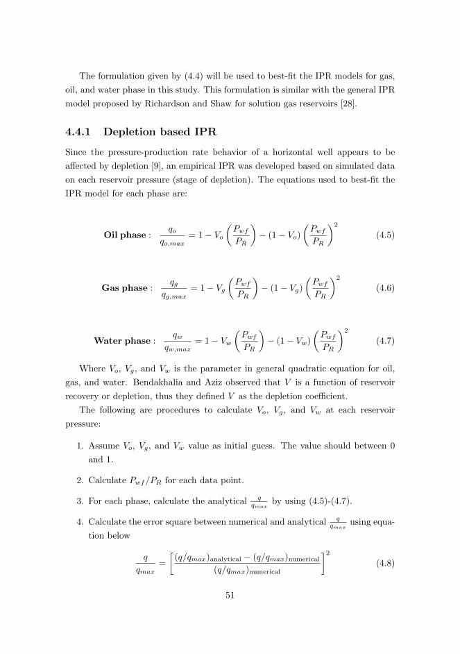
4.12 Vg and SSQg as a Function of Reservoir Pressure. . . . . . . . . . . . 53

4.13 Vw and SSQw as a Function of Reservoir Pressure. . . . . . . . . . . 53

4.14 Comparison of Generalized IPR with Numerical Data for Oil Phase. 55

4.15 Comparison of Generalized IPR with Numerical Data for Gas Phase. 56

4.16 Comparison of Generalized IPR with Numerical Data for Water Phase. 56

viii

Chapter 1

INTRODUCTION

1.1 Background

Horizontal well have become a popular option for oil production in petroleum

industry. This type of well could accelerate oil production, control coning, and

in some cases could turn uneconomical reserves into a commercial one (i.e. in

low permeability reservoir, reservoir with viscous oil, thin reservoir, etc.). Thin

reservoir is a very good candidate for horizontal well since the increases in formation

thickness decrease the productivity ratio of the horizontal well to vertical well [13].

In reservoir with thin oil column, sandwiched between big gas cap and aquifer,

gas and water coning most likely will occurs during oil production. Since the

critical rates usually very low (and un-economic), the well usually produce at rate

higher than the critical rates. This makes coning problems un-avoidable. In this

condition, a three-phase flow (gas-oil-water) exists in production stream.

Inflow performance in a horizontal well could be estimate using an analytical

solution or empirical IPR. The analytical solutions are based on single-phase flow

principles and may not be appropriate for three-phase, gas-oil-water flow. Thus,

an empirical IPR solution might be preferable. As author knowledge, there have

not been any publications presenting IPR model for horizontal well with gas and

water coning problem. The main objective of this study is to address this gap

by developing an IPR model for horizontal well producing from thin oil reservoir

underlying gas cap and overlaying aquifer, with gas and water coning problem.

1

1.2 Study Objectives

The main objective of this study was to develop Inflow Performance Relationship

(IPR) for horizontal well producing from oil reservoir with gas and water coning

problem. Both dimensional and dimensionless IPR with its best-fit equations were

presented in this study.

The other objectives are to conduct a sensitivity study to understand the effect

of several parameters to gas and water coning behavior and to do well placement

optimization and coning collapse study.

1.3 Description of Employed Software

1.3.1 Sensor

Sensor, which is stands for System for Efficient Numerical Simulation of Oil Re-

covery, is the compositional and black oil reservoir simulation software that was

developed by Coats Engineering, Inc. This software is a generalized 3D numerical

model used by engineers to optimize oil and gas recovery processes through simula-

tion of compositional and black oil fluid flow in single porosity, dual porosity, and

dual permeability petroleum reservoir [1].

This numerical simulation was used to run the model and extract all values

needed to generate IPR curves. Sensor was also used to study the gas and water

coning behavior and how it is affect production performance.

1.3.2 Pipe-It

Pipe-It is a unique application generated by Petrostreamz, a software company

developed at PERA AS. This software allows the user to graphically and compu-

tationally integrate models and optimize petroleum assets [2]. Pipe-It can chains

several applications in series and parallel and launch any software on any operating

system.

In this study, Pipe-It is used to simplify the Sensor run. MapLinkz and Linkz

applications inside Pipe-It were also used in extracting data from simulation output,

thus avoiding lots of manual copy and paste work that can be time consuming.

2

Chapter 2

MODEL INITIALIZATION

2.1 Data Acquisition and Preparation

One objective in this study is to observe gas and water coning behavior in a reservoir

with horizontal well producing from thin oil zone sandwiched between big gas cap

and aquifer. A further IPR curves will also be constructed for this certain reservoir.

Thus, a base case model that represents this condition need to be generated.

For reference, we use the three-well Sensor compositional model that was gener-

ated by Dr. Alexander Juell. This reference model contains rock and fluid proper-

ties which are similar to Troll field; a natural gas an oil field in North sea that has

thin oil rims between large gas cap and active aquifer. Several modifications were

made on this reference model to generate the base case, this which the intention

to have reservoir model that suit the objectives of the project.

The reference model is a fully implicit 3D Cartesian model with 3278 ft, 3280 ft,

and 160 ft; total length in x, y, and z-direction respectively. This model use total

number of grid of 1480 (Nx = 40, Ny = 1, Nz = 37). The horizontal well extends

through the full length of reservoir in y-direction with only one grid number along

the horizontal section, this make the model become 2D problems with uniform

pressure (influx) along the well.

3

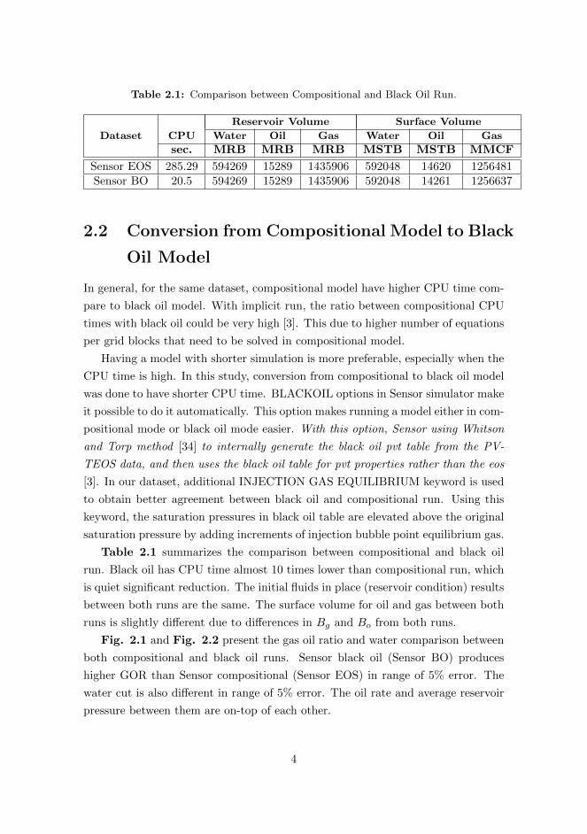
Table 2.1: Comparison between Compositional and Black Oil Run.

Reservoir Volume Surface Volume

Dataset CPU Water Oil Gas Water Oil Gas

sec. MRB MRB MRB MSTB MSTB MMCF

Sensor EOS 285.29 594269 15289 1435906 592048 14620 1256481Sensor BO 20.5 594269 15289 1435906 592048 14261 1256637

2.2 Conversion from Compositional Model to Black

Oil Model

In general, for the same dataset, compositional model have higher CPU time com-

pare to black oil model. With implicit run, the ratio between compositional CPU

times with black oil could be very high [3]. This due to higher number of equations

per grid blocks that need to be solved in compositional model.

Having a model with shorter simulation is more preferable, especially when the

CPU time is high. In this study, conversion from compositional to black oil model

was done to have shorter CPU time. BLACKOIL options in Sensor simulator make

it possible to do it automatically. This option makes running a model either in com-

positional mode or black oil mode easier. With this option, Sensor using Whitson

and Torp method [34] to internally generate the black oil pvt table from the PV-

TEOS data, and then uses the black oil table for pvt properties rather than the eos

[3]. In our dataset, additional INJECTION GAS EQUILIBRIUM keyword is used

to obtain better agreement between black oil and compositional run. Using this

keyword, the saturation pressures in black oil table are elevated above the original

saturation pressure by adding increments of injection bubble point equilibrium gas.

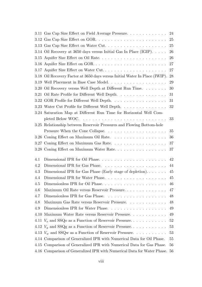
Table 2.1 summarizes the comparison between compositional and black oil

run. Black oil has CPU time almost 10 times lower than compositional run, which

is quiet significant reduction. The initial fluids in place (reservoir condition) results

between both runs are the same. The surface volume for oil and gas between both

runs is slightly different due to differences in Bg and Bo from both runs.

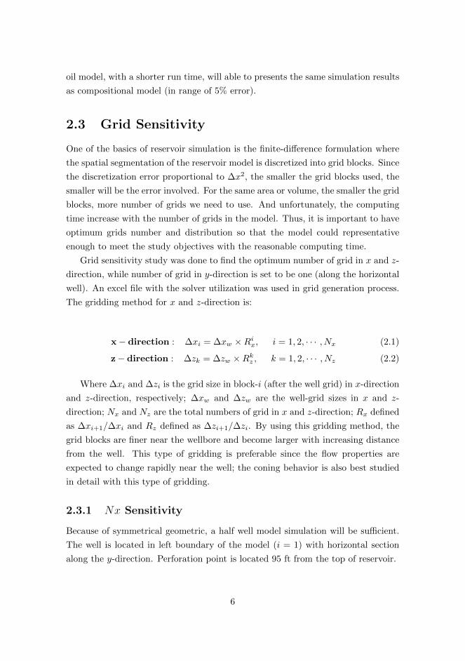
Fig. 2.1 and Fig. 2.2 present the gas oil ratio and water comparison between

both compositional and black oil runs. Sensor black oil (Sensor BO) produces

higher GOR than Sensor compositional (Sensor EOS) in range of 5% error. The

water cut is also different in range of 5% error. The oil rate and average reservoir

pressure between them are on-top of each other.

4

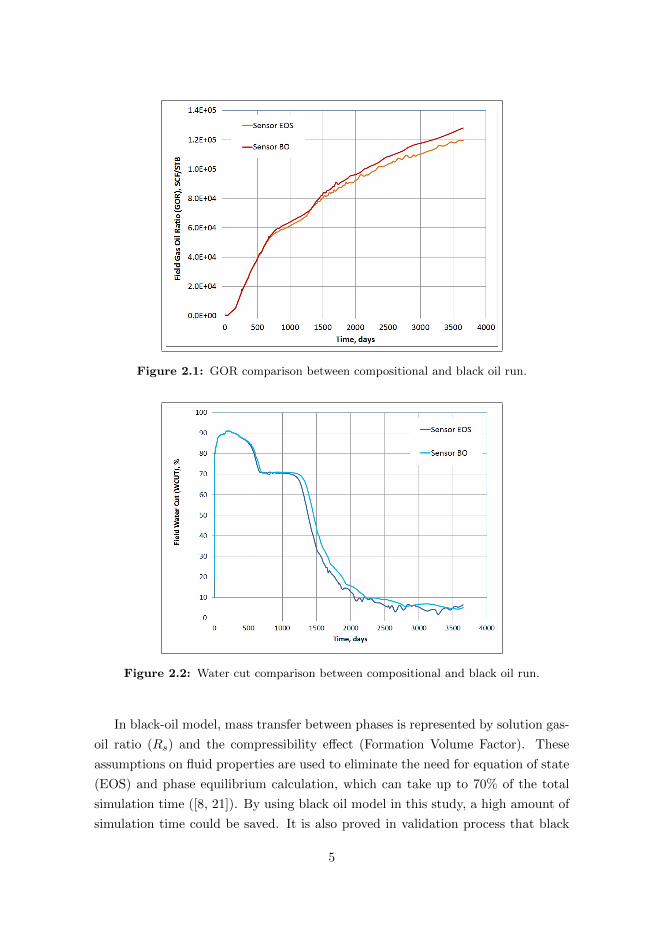
Figure 2.1: GOR comparison between compositional and black oil run.

Figure 2.2: Water cut comparison between compositional and black oil run.

In black-oil model, mass transfer between phases is represented by solution gas-

oil ratio (Rs) and the compressibility effect (Formation Volume Factor). These

assumptions on fluid properties are used to eliminate the need for equation of state

(EOS) and phase equilibrium calculation, which can take up to 70% of the total

simulation time ([8, 21]). By using black oil model in this study, a high amount of

simulation time could be saved. It is also proved in validation process that black

5

oil model, with a shorter run time, will able to presents the same simulation results

as compositional model (in range of 5% error).

2.3 Grid Sensitivity

One of the basics of reservoir simulation is the finite-difference formulation where

the spatial segmentation of the reservoir model is discretized into grid blocks. Since

the discretization error proportional to ∆x2, the smaller the grid blocks used, the

smaller will be the error involved. For the same area or volume, the smaller the grid

blocks, more number of grids we need to use. And unfortunately, the computing

time increase with the number of grids in the model. Thus, it is important to have

optimum grids number and distribution so that the model could representative

enough to meet the study objectives with the reasonable computing time.

Grid sensitivity study was done to find the optimum number of grid in x and z-

direction, while number of grid in y-direction is set to be one (along the horizontal

well). An excel file with the solver utilization was used in grid generation process.

The gridding method for x and z-direction is:

x− direction : ∆xi = ∆xw ×Rix, i = 1, 2, · · · , Nx (2.1)

z− direction : ∆zk = ∆zw ×Rkz , k = 1, 2, · · · , Nz (2.2)

Where ∆xi and ∆zi is the grid size in block-i (after the well grid) in x-direction

and z-direction, respectively; ∆xw and ∆zw are the well-grid sizes in x and z-

direction; Nx and Nz are the total numbers of grid in x and z-direction; Rx defined

as ∆xi+1/∆xi and Rz defined as ∆zi+1/∆zi. By using this gridding method, the

grid blocks are finer near the wellbore and become larger with increasing distance

from the well. This type of gridding is preferable since the flow properties are

expected to change rapidly near the well; the coning behavior is also best studied

in detail with this type of gridding.

2.3.1 Nx Sensitivity

Because of symmetrical geometric, a half well model simulation will be sufficient.

The well is located in left boundary of the model (i = 1) with horizontal section

along the y-direction. Perforation point is located 95 ft from the top of reservoir.

6

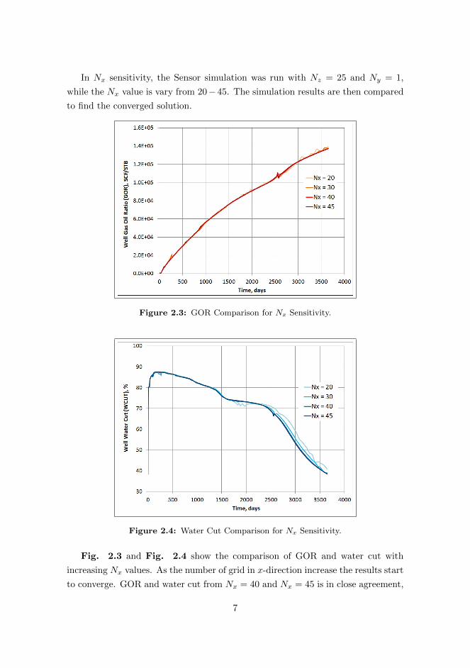
In Nx sensitivity, the Sensor simulation was run with Nz = 25 and Ny = 1,

while the Nx value is vary from 20− 45. The simulation results are then compared

to find the converged solution.

Figure 2.3: GOR Comparison for Nx Sensitivity.

Figure 2.4: Water Cut Comparison for Nx Sensitivity.

Fig. 2.3 and Fig. 2.4 show the comparison of GOR and water cut with

increasing Nx values. As the number of grid in x-direction increase the results start

to converge. GOR and water cut from Nx = 40 and Nx = 45 is in close agreement,

7

thus it could be conclude that with Nx = 40 we already have a converge solution.

For future work in this study, Nx = 40 will be used in the model.

2.3.2 NZTOP and NZBOTTOM Sensitivity

Figure 2.5: GOR Comparison for NZTOP Sensitivity.

Figure 2.6: Water Cut Comparison for NZTOP Sensitivity.

8

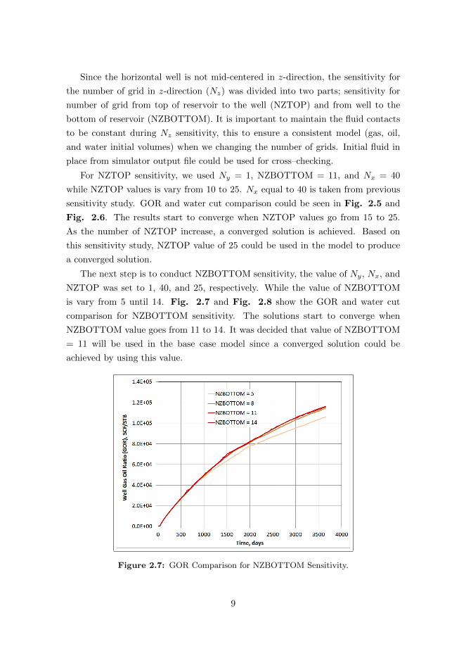
Since the horizontal well is not mid-centered in z-direction, the sensitivity for

the number of grid in z-direction (Nz) was divided into two parts; sensitivity for

number of grid from top of reservoir to the well (NZTOP) and from well to the

bottom of reservoir (NZBOTTOM). It is important to maintain the fluid contacts

to be constant during Nz sensitivity, this to ensure a consistent model (gas, oil,

and water initial volumes) when we changing the number of grids. Initial fluid in

place from simulator output file could be used for cross–checking.

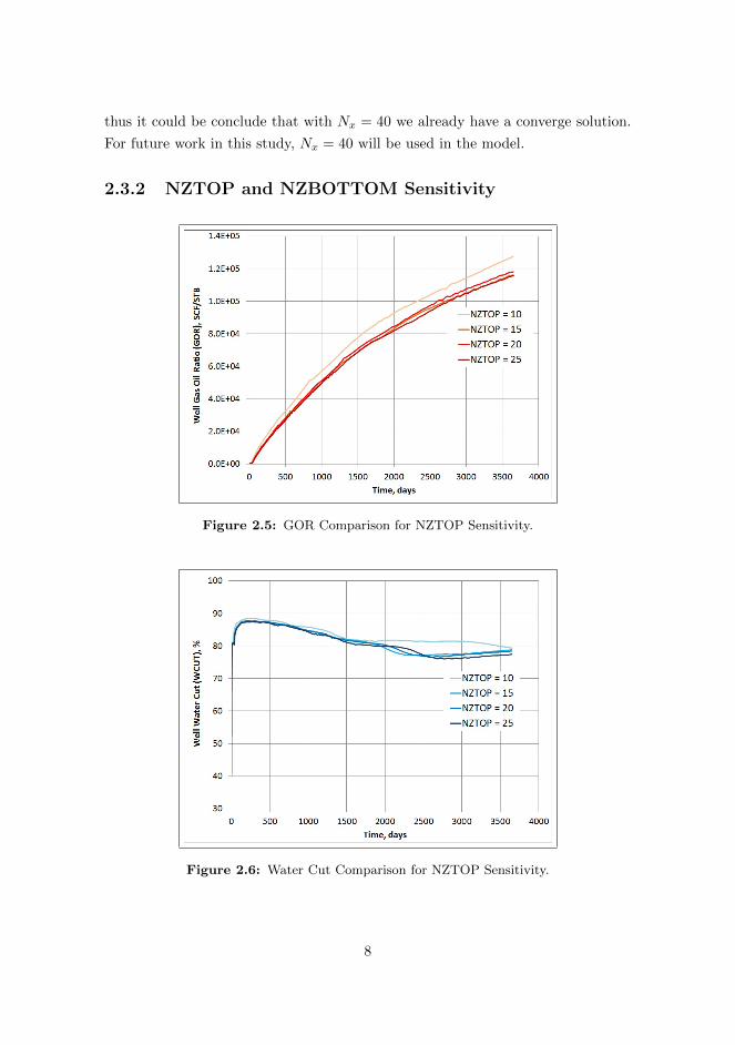
For NZTOP sensitivity, we used Ny = 1, NZBOTTOM = 11, and Nx = 40

while NZTOP values is vary from 10 to 25. Nx equal to 40 is taken from previous

sensitivity study. GOR and water cut comparison could be seen in Fig. 2.5 and

Fig. 2.6. The results start to converge when NZTOP values go from 15 to 25.

As the number of NZTOP increase, a converged solution is achieved. Based on

this sensitivity study, NZTOP value of 25 could be used in the model to produce

a converged solution.

The next step is to conduct NZBOTTOM sensitivity, the value of Ny, Nx, and

NZTOP was set to 1, 40, and 25, respectively. While the value of NZBOTTOM

is vary from 5 until 14. Fig. 2.7 and Fig. 2.8 show the GOR and water cut

comparison for NZBOTTOM sensitivity. The solutions start to converge when

NZBOTTOM value goes from 11 to 14. It was decided that value of NZBOTTOM

= 11 will be used in the base case model since a converged solution could be

achieved by using this value.

Figure 2.7: GOR Comparison for NZBOTTOM Sensitivity.

9

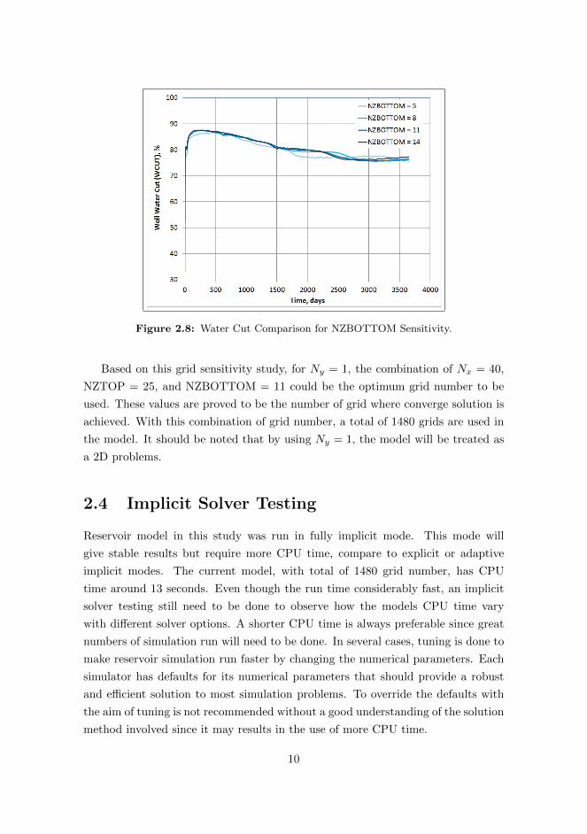
Figure 2.8: Water Cut Comparison for NZBOTTOM Sensitivity.

Based on this grid sensitivity study, for Ny = 1, the combination of Nx = 40,

NZTOP = 25, and NZBOTTOM = 11 could be the optimum grid number to be

used. These values are proved to be the number of grid where converge solution is

achieved. With this combination of grid number, a total of 1480 grids are used in

the model. It should be noted that by using Ny = 1, the model will be treated as

a 2D problems.

2.4 Implicit Solver Testing

Reservoir model in this study was run in fully implicit mode. This mode will

give stable results but require more CPU time, compare to explicit or adaptive

implicit modes. The current model, with total of 1480 grid number, has CPU

time around 13 seconds. Even though the run time considerably fast, an implicit

solver testing still need to be done to observe how the models CPU time vary

with different solver options. A shorter CPU time is always preferable since great

numbers of simulation run will need to be done. In several cases, tuning is done to

make reservoir simulation run faster by changing the numerical parameters. Each

simulator has defaults for its numerical parameters that should provide a robust

and efficient solution to most simulation problems. To override the defaults with

the aim of tuning is not recommended without a good understanding of the solution

method involved since it may results in the use of more CPU time.

10

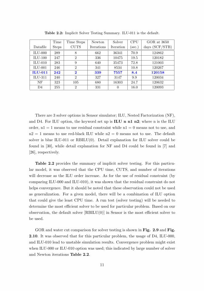
Table 2.2: Implicit Solver Testing Summary. ILU-011 is the default.

Time Time Steps Newton Solver CPU GOR at 3650

Datafile Steps CUTS Iterations Iteration (sec.) days (SCF/STB)

ILU-000 289 8 662 36341 70.9 124862

ILU-100 247 2 336 10475 19.5 120182

ILU-010 283 9 640 35473 72.8 121003

ILU-001 246 2 341 8534 10.8 120267

ILU-011 242 2 339 7557 8.4 120158

ILU-311 240 2 327 3147 9.9 120034

NF 323 105 680 16303 24.7 120632

D4 255 2 331 0 16.0 120093

There are 3 solver options in Sensor simulator; ILU, Nested Factorization (NF),

and D4. For ILU option, the keyword set up is ILU n n1 n2; where n is the ILU

order, n1 = 1 means to use residual constraint while n1 = 0 means not to use, and

n2 = 1 means to use red-black ILU while n2 = 0 means not to use. The default

solver is blue ILU-011 or RBILU(0). Detail explanation for ILU solver could be

found in [30], while detail explanation for NF and D4 could be found in [7] and

[26], respectively.

Table 2.2 provides the summary of implicit solver testing. For this particu-

lar model, it was observed that the CPU time, CUTS, and number of iterations

will decrease as the ILU order increase. As for the use of residual constraint (by

comparing ILU-000 and ILU-010), it was shown that the residual constraint do not

helps convergence. But it should be noted that these observation could not be used

as generalization. For a given model, there will be a combination of ILU option

that could give the least CPU time. A run test (solver testing) will be needed to

determine the most efficient solver to be used for particular problem. Based on our

observation, the default solver [RBILU(0)] in Sensor is the most efficient solver to

be used.

GOR and water cut comparison for solver testing is shown in Fig. 2.9 and Fig.

2.10. It was observed that for this particular problem, the usage of D4, ILU-000,

and ILU-010 lead to unstable simulation results. Convergence problem might exist

when ILU-000 or ILU-010 option was used; this indicated by large number of solver

and Newton iterations Table 2.2.

11

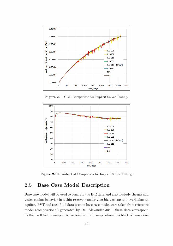
Figure 2.9: GOR Comparison for Implicit Solver Testing.

Figure 2.10: Water Cut Comparison for Implicit Solver Testing.

2.5 Base Case Model Description

Base case model will be used to generate the IPR data and also to study the gas and

water coning behavior in a thin reservoir underlying big gas cap and overlaying an

aquifer. PVT and rock-fluid data used in base case model were taken from reference

model (compositional) generated by Dr. Alexander Juell, these data correspond

to the Troll field example. A conversion from compositional to black oil was done

12

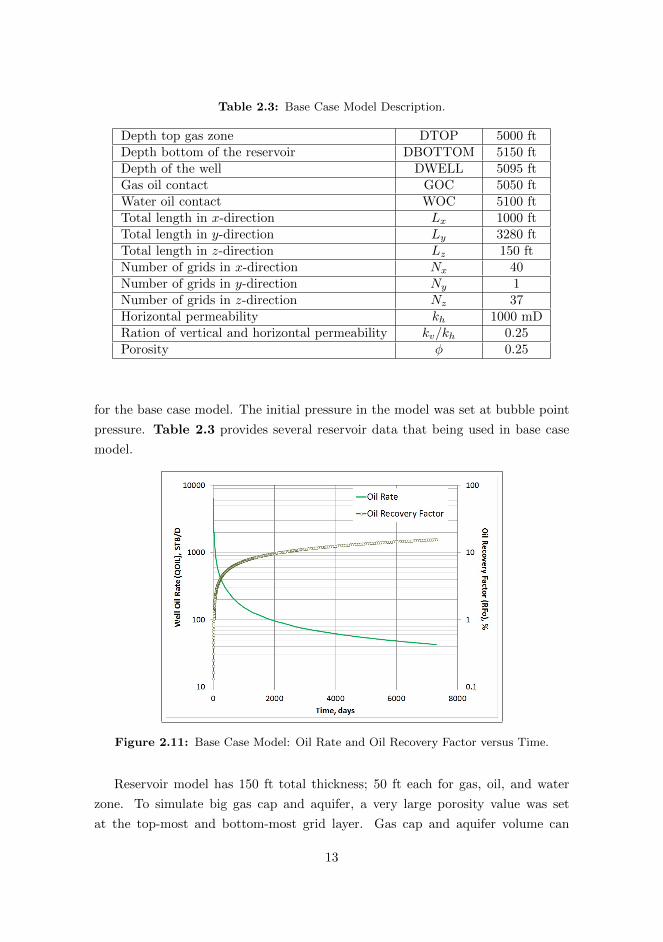
Table 2.3: Base Case Model Description.

Depth top gas zone DTOP 5000 ftDepth bottom of the reservoir DBOTTOM 5150 ftDepth of the well DWELL 5095 ftGas oil contact GOC 5050 ftWater oil contact WOC 5100 ftTotal length in x-direction Lx 1000 ftTotal length in y-direction Ly 3280 ftTotal length in z-direction Lz 150 ftNumber of grids in x-direction Nx 40Number of grids in y-direction Ny 1Number of grids in z-direction Nz 37Horizontal permeability kh 1000 mDRation of vertical and horizontal permeability kv/kh 0.25Porosity φ 0.25

for the base case model. The initial pressure in the model was set at bubble point

pressure. Table 2.3 provides several reservoir data that being used in base case

model.

Figure 2.11: Base Case Model: Oil Rate and Oil Recovery Factor versus Time.

Reservoir model has 150 ft total thickness; 50 ft each for gas, oil, and water

zone. To simulate big gas cap and aquifer, a very large porosity value was set

at the top-most and bottom-most grid layer. Gas cap and aquifer volume can

13

Figure 2.12: Base Case Model: Bottom-hole Pressure versus Time.

be adjusted by changing the thickness of these layers. One horizontal producer

well were completed along y-direction, located at grid (i = 1, j = 1, k = 26), and

perforated 5 ft above WOC. This well produces at minimum BHP of 1500 psia and

maximum oil rate of 10000 STB/D.

Fig. 2.11 and Fig. 2.12 present the oil rate, oil recovery factor, and flowing

bottom-hole pressure versus time for base case model. The oil rate decrease rapidly

in the first two years; after 20 years of production the oil rate go down to 43 STB/d.

Major recoveries was achieved at first 10 years, afterward, the oil recovery increase

in a slow rate and achieve 16% after 20 years of production. The reservoir pressure

decreases ±300 psia in 20 years.

Gas and water breakthrough occurs in the early period of production. Severe

gas coning indicated by a rapid increase of GOR in the production well (Fig.

2.13). The water breakthrough indicated by sharp increase of water, after some

times the water cut decrease and become relatively stable at 80% (Fig. 2.14).

When the well starts producing higher than the critical rate; the coning (gas and

water) occurs. High pressure from big gas cap pushes the oil down to water zone.

In consequences; the GOR increases rapidly and the oil rate decreases. While

the water cut, after the breakthrough and sharp increase in water cut occurs, gas

coning start to dominate the flow (due to high pressure from gas cap). This might

be the reason why the water cut decrease after breakthrough happened.

14

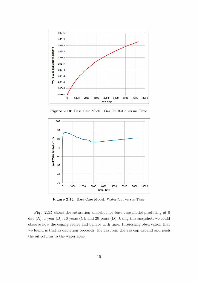
Figure 2.13: Base Case Model: Gas Oil Ratio versus Time.

Figure 2.14: Base Case Model: Water Cut versus Time.

Fig. 2.15 shows the saturation snapshot for base case model producing at 0

day (A), 1 year (B), 10 years (C), and 20 years (D). Using this snapshot, we could

observe how the coning evolve and behave with time. Interesting observation that

we found is that as depletion proceeds, the gas from the gas cap expand and push

the oil column to the water zone.

15

Figure 2.15: Saturation Snapshot of Base Case Model (IK-cross section).

16

Chapter 3

WATER AND GAS

CONING IN HORIZONTAL

WELL

3.1 Introduction

Several analytical studies indicate that horizontal well usually have higher produc-

tivity than vertical well, this mainly due to longer length open to flow [8, 11, 24].

In a thin oil reservoir, horizontal wells were proposed as an alternative to vertical

wells. Coning occurs when a pressure gradient near the perforated interval exceeds

the gravity head from fluid density differences. The long length, increased areal

sweep and increased productivity of the horizontal well could reduce this pressure

gradient; thus reducing the coning problems and improve the oil recovery.

In reservoir with thin oil column, sandwiched between big gas cap and aquifer,

gas and water coning most likely will occurs during oil production. Since the critical

rates usually very low (and un-economic), the well usually produce at rate higher

than the critical rates. This makes coning problems un-avoidable. In this project,

several sensitivity studies were done to better understand the coning behavior for

horizontal well produce from thin oil reservoir underlying big gas cap and overlaying

an aquifer.

17

In general, coning behavior depends on thickness of oil column, density contrast

between oil and coning fluids, oil viscosity, effective permeability, and the size of

gas cap and/or aquifer strength. In this chapter, only last three parameters will

be discussed in detail based on sensitivity results.

3.2 Permeability Sensitivity

Permeability sensitivity divided into 2 sections, horizontal permeability sensitivity

and ratio of vertical to horizontal permeability sensitivity. The base case model

will be used with only one parameter is changed per simulation run. The objective

is to observe the effect of permeability on water and gas coning in thin oil reservoir

sandwiched between gas cap and aquifer.

3.2.1 Horizontal Permeability Sensitivity

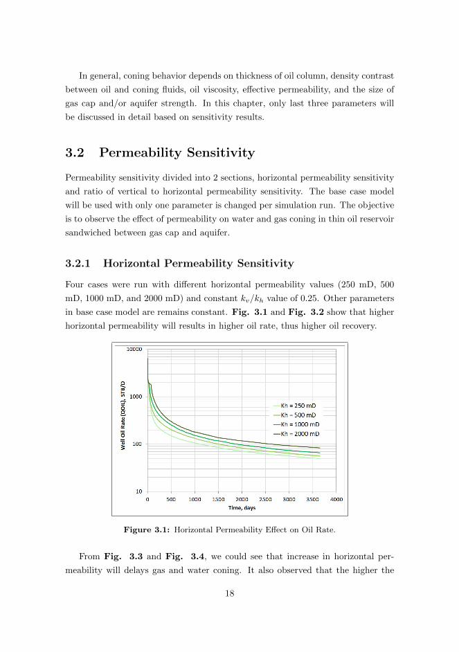
Four cases were run with different horizontal permeability values (250 mD, 500

mD, 1000 mD, and 2000 mD) and constant kv/kh value of 0.25. Other parameters

in base case model are remains constant. Fig. 3.1 and Fig. 3.2 show that higher

horizontal permeability will results in higher oil rate, thus higher oil recovery.

Figure 3.1: Horizontal Permeability Effect on Oil Rate.

From Fig. 3.3 and Fig. 3.4, we could see that increase in horizontal per-

meability will delays gas and water coning. It also observed that the higher the

18

Figure 3.2: Oil Recovery Factor at 10 years versus Horizontal Permeability.

horizontal permeability, the lower the GOR and/or water cut after breakthrough.

In a reservoir with high horizontal permeability, the fluids will tend to flow in hor-

izontal direction than vertical direction. This will reduce the tendency of gas and

water to cone into the well. In consequences, the breakthrough time and critical

rate will be higher and the coning-fluid production after breakthrough will be lower.

Figure 3.3: Horizontal Permeability Effect on Water Cut.

19

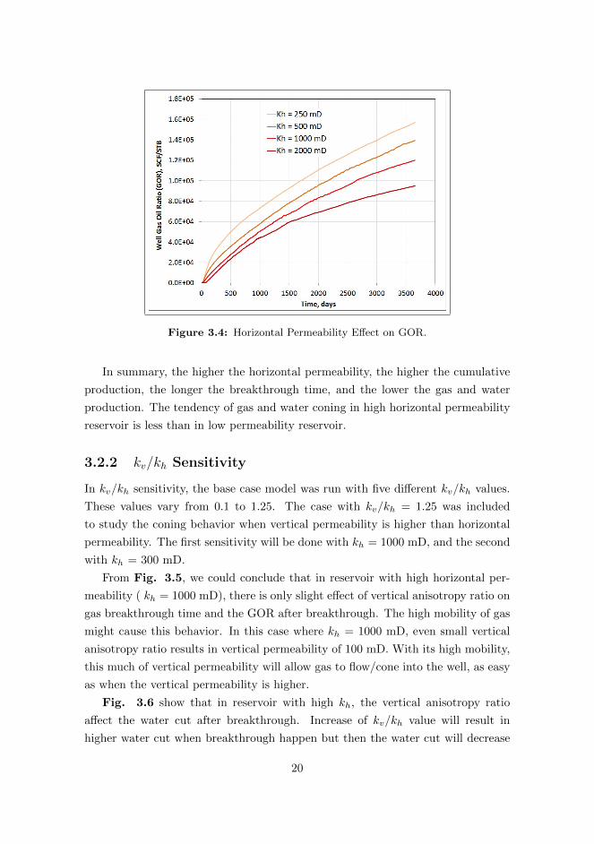
Figure 3.4: Horizontal Permeability Effect on GOR.

In summary, the higher the horizontal permeability, the higher the cumulative

production, the longer the breakthrough time, and the lower the gas and water

production. The tendency of gas and water coning in high horizontal permeability

reservoir is less than in low permeability reservoir.

3.2.2 kv/kh Sensitivity

In kv/kh sensitivity, the base case model was run with five different kv/kh values.

These values vary from 0.1 to 1.25. The case with kv/kh = 1.25 was included

to study the coning behavior when vertical permeability is higher than horizontal

permeability. The first sensitivity will be done with kh = 1000 mD, and the second

with kh = 300 mD.

From Fig. 3.5, we could conclude that in reservoir with high horizontal per-

meability ( kh = 1000 mD), there is only slight effect of vertical anisotropy ratio on

gas breakthrough time and the GOR after breakthrough. The high mobility of gas

might cause this behavior. In this case where kh = 1000 mD, even small vertical

anisotropy ratio results in vertical permeability of 100 mD. With its high mobility,

this much of vertical permeability will allow gas to flow/cone into the well, as easy

as when the vertical permeability is higher.

Fig. 3.6 show that in reservoir with high kh, the vertical anisotropy ratio

affect the water cut after breakthrough. Increase of kv/kh value will result in

higher water cut when breakthrough happen but then the water cut will decrease

20

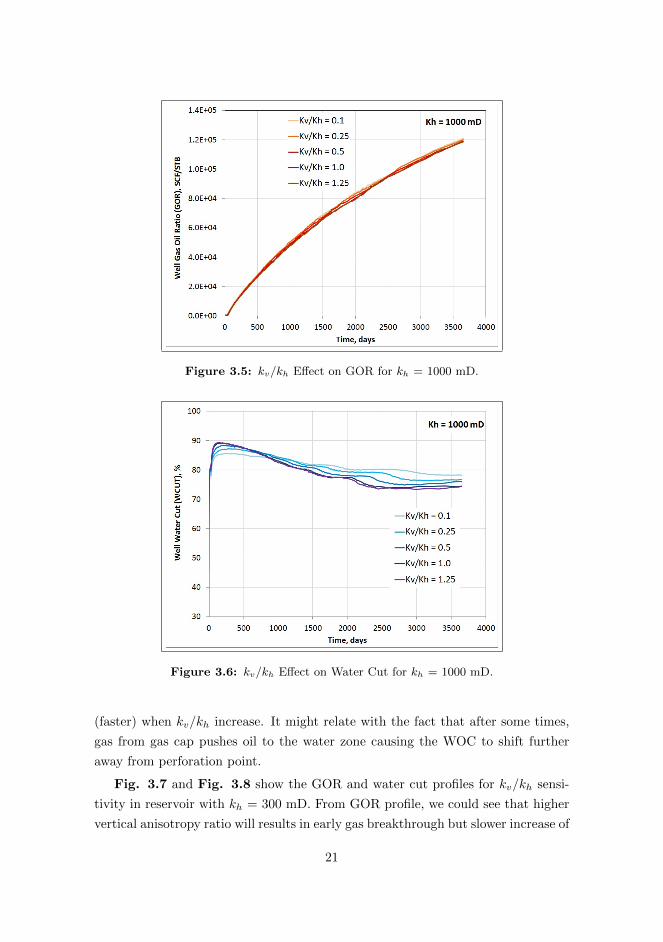
Figure 3.5: kv/kh Effect on GOR for kh = 1000 mD.

Figure 3.6: kv/kh Effect on Water Cut for kh = 1000 mD.

(faster) when kv/kh increase. It might relate with the fact that after some times,

gas from gas cap pushes oil to the water zone causing the WOC to shift further

away from perforation point.

Fig. 3.7 and Fig. 3.8 show the GOR and water cut profiles for kv/kh sensi-

tivity in reservoir with kh = 300 mD. From GOR profile, we could see that higher

vertical anisotropy ratio will results in early gas breakthrough but slower increase of

21

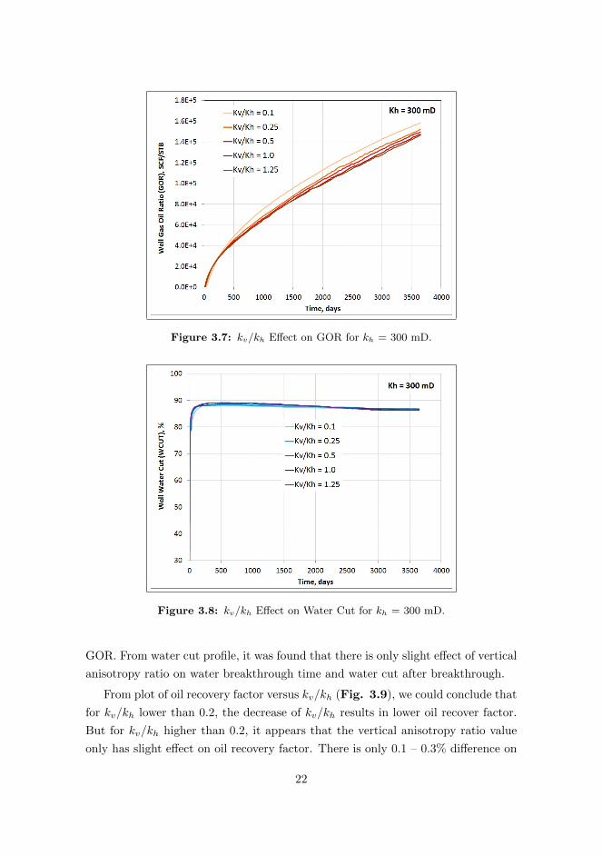
Figure 3.7: kv/kh Effect on GOR for kh = 300 mD.

Figure 3.8: kv/kh Effect on Water Cut for kh = 300 mD.

GOR. From water cut profile, it was found that there is only slight effect of vertical

anisotropy ratio on water breakthrough time and water cut after breakthrough.

From plot of oil recovery factor versus kv/kh (Fig. 3.9), we could conclude that

for kv/kh lower than 0.2, the decrease of kv/kh results in lower oil recover factor.

But for kv/kh higher than 0.2, it appears that the vertical anisotropy ratio value

only has slight effect on oil recovery factor. There is only 0.1 – 0.3% difference on

22

Figure 3.9: Oil Recovery at 3650 days versus kv/kh for Different kh Values.

oil recovery for kv/kh values of 0.1 to 1.25. These conclusion apply for reservoir

with kh = 1000 mD and kh = 300 mD.

3.3 Gas Cap and Aquifer Size Sensitivity

To better understand the coning behavior in thin oil reservoir underlying a gas cap

and overlaying an aquifer, a sensitivity of gas cap and aquifer size was done. The

size of gas cap and aquifer are represented by the initial volume of gas and water.

In Sensor data file, the size of gas cap and aquifer was changed by modifying the

gas cap and aquifer height.

Gas cap size sensitivity will be discussed first in this section. The sensitivity was

done by using the base case model and run it using Sensor with different gas cap

height value per simulation run. Results from this sensitivity study are presented

below.

Fig. 3.10 shows that the size of gas cap only has slight effect the oil rate.

Increase in gas cap size will results in lower oil rate. The existence of gas cap

usually help in reservoir pressure support/pressure maintenance. As we can see

from Fig. 3.11, bigger gas cap size will provide more pressure support in reservoir.

Reservoir pressure decrease faster when the gas cap size is smaller.

Fig. 3.12 and Fig. 3.13 show that the gas cap size does not affect the water

and gas breakthrough time. Different gas cap sizes give approximately the same

23

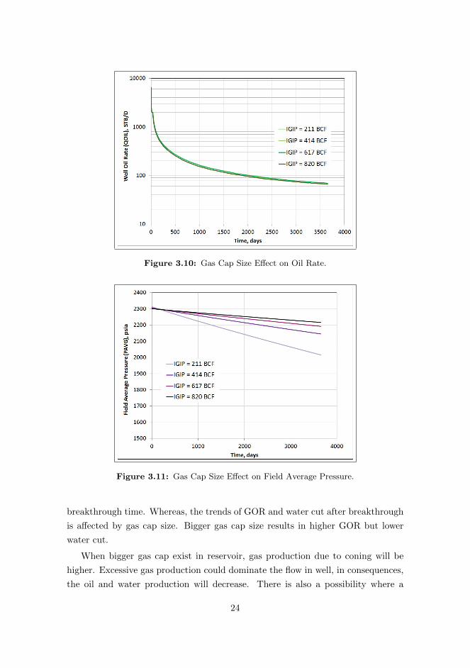
Figure 3.10: Gas Cap Size Effect on Oil Rate.

Figure 3.11: Gas Cap Size Effect on Field Average Pressure.

breakthrough time. Whereas, the trends of GOR and water cut after breakthrough

is affected by gas cap size. Bigger gas cap size results in higher GOR but lower

water cut.

When bigger gas cap exist in reservoir, gas production due to coning will be

higher. Excessive gas production could dominate the flow in well, in consequences,

the oil and water production will decrease. There is also a possibility where a

24

Figure 3.12: Gas Cap Size Effect on GOR.

Figure 3.13: Gas Cap Size Effect on Water Cut.

bigger gas cap could push oil further down into the water zone. When this happen,

the distance between perforation point and WOC will be longer thus resulting in

lower water production or lower water cut.

Increase in gas cap size will results in lower oil recovery factor (Fig. 3.14).

Even though bigger gas cap can give more pressure support in reservoir, it can also

cause more gas production from coning. When the gas dominates flow into the well,

25

the oil production will decrease. In consequences the cumulative oil production (oil

recovery) is lower.

Figure 3.14: Oil Recovery at 3650 days versus Initial Gas In Place (IGIP).

Figure 3.15: Aquifer Size Effect on Oil Rate.

Aquifer size sensitivity will be discussed in this section. The sensitivity was done

by using the base case model and run it using Sensor with different aquifer size per

simulation run. The aquifer size was changed by modifying the bottom-most grid

block height.

26

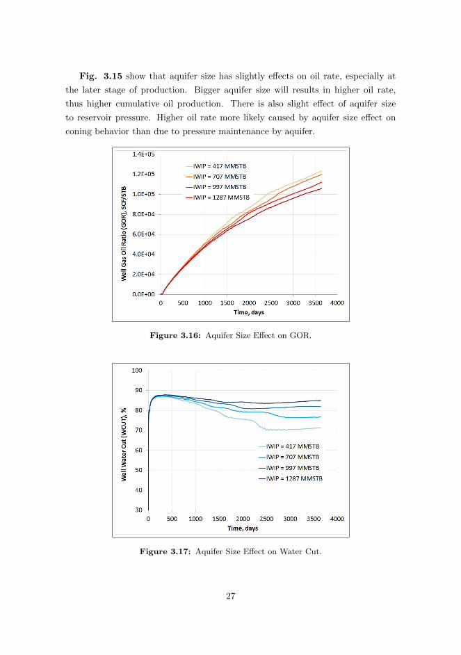
Fig. 3.15 show that aquifer size has slightly effects on oil rate, especially at

the later stage of production. Bigger aquifer size will results in higher oil rate,

thus higher cumulative oil production. There is also slight effect of aquifer size

to reservoir pressure. Higher oil rate more likely caused by aquifer size effect on

coning behavior than due to pressure maintenance by aquifer.

Figure 3.16: Aquifer Size Effect on GOR.

Figure 3.17: Aquifer Size Effect on Water Cut.

27

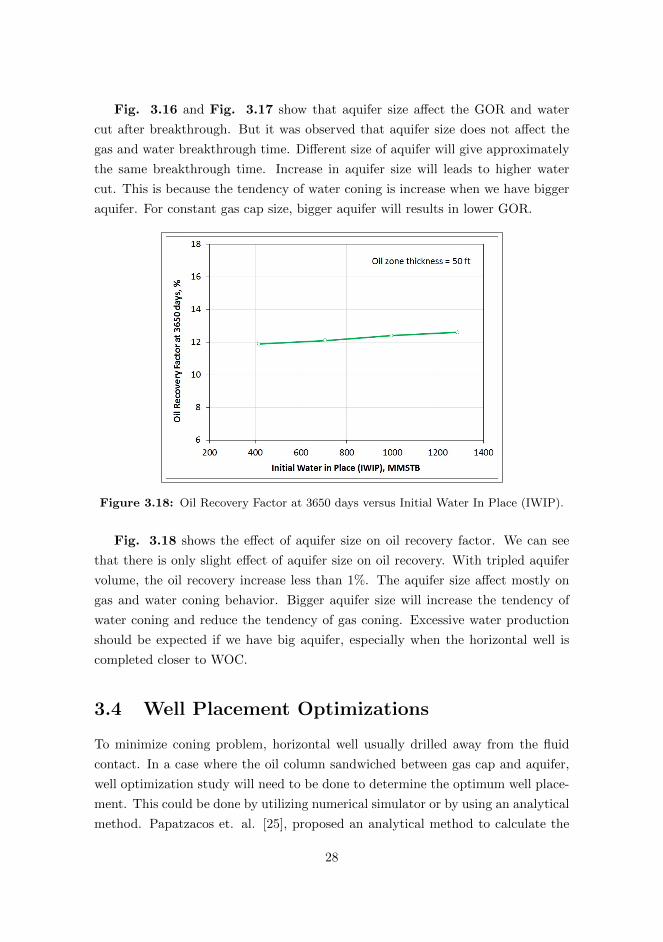
Fig. 3.16 and Fig. 3.17 show that aquifer size affect the GOR and water

cut after breakthrough. But it was observed that aquifer size does not affect the

gas and water breakthrough time. Different size of aquifer will give approximately

the same breakthrough time. Increase in aquifer size will leads to higher water

cut. This is because the tendency of water coning is increase when we have bigger

aquifer. For constant gas cap size, bigger aquifer will results in lower GOR.

Figure 3.18: Oil Recovery Factor at 3650 days versus Initial Water In Place (IWIP).

Fig. 3.18 shows the effect of aquifer size on oil recovery factor. We can see

that there is only slight effect of aquifer size on oil recovery. With tripled aquifer

volume, the oil recovery increase less than 1%. The aquifer size affect mostly on

gas and water coning behavior. Bigger aquifer size will increase the tendency of

water coning and reduce the tendency of gas coning. Excessive water production

should be expected if we have big aquifer, especially when the horizontal well is

completed closer to WOC.

3.4 Well Placement Optimizations

To minimize coning problem, horizontal well usually drilled away from the fluid

contact. In a case where the oil column sandwiched between gas cap and aquifer,

well optimization study will need to be done to determine the optimum well place-

ment. This could be done by utilizing numerical simulator or by using an analytical

method. Papatzacos et. al. [25], proposed an analytical method to calculate the

28

optimum well placement, where the gas and water coning will breakthrough at

same time. But practically, delaying a gas breakthrough is the main concern. Over

time, gas breakthrough can dominate flow in the well and cause reduction in oil

rate. Excessive gas production from gas cap can also cause rapid pressure decline

in reservoir. Fig. 3.19 shows the horizontal well placement in our base case model.

The well was located 5 ft away from WOC and 45 ft away from GOC.

Figure 3.19: Well Placement in Base Case Model.

Base case model was run with different well depth using Sensor. The oil recovery

factor for each well depth at 1, 5, 10, 20, and 30 years was recorded and plotted on

XY -chart Fig. 3.20. An interesting observation from this figure is that the trends

of oil recovery factor changes with time. If we only consider one year production,

the optimum well placement is in the lower one-third section of the oil leg. In

field application, usually this is where the horizontal well is drilled. But the oil

recovery trends are changes with time; in a long production period, it appears to

be beneficial to place horizontal well in upper section of the oil leg. If we consider

20 years of production, the optimum well placement will be around upper two-fifth

section of the oil leg.

These observations should not be made as generalization since it was generated

only using one set data of reservoir model. There might be different trends of oil

recovery factor for different reservoir and horizontal well configuration. We recom-

mend generating the plot based on your particular reservoir, development plan, and

well configuration data; and use it as a tool to help in deciding the optimum well

29

placement. Several factors that might effect on optimum well placement are oil flow

rate, oil viscosity; oil FVF, density difference between reservoir fluid, perforation

interval lengths, mobility ratio, and the gas cap and aquifer size [32].

Figure 3.20: Oil Recovery versus Well Depth at Different Run Time.

The production profiles of horizontal well (Fig. 3.21 – Fig. 3.23) could help

to explain the trends that we saw on oil recovery plot versus well depth. When

the well is placed closer to WOC, the water production will increase significantly

at early time. The gas coning will be delayed but after the breakthrough happen,

the gas production will increase rapidly with time. These results in decreasing

oil rate. And when the well is placed closer to GOC, the gas breakthrough will

happen at early time and the gas production will increase with time, but less rapid

than the gas production from the well closer to WOC. The water breakthrough

will be delayed, but after the breakthrough happen water production will increase.

Water cut is higher for the well closer to WOC. The oil rate will decrease with

time when the coning occurs. But since there are less gas and water coning, the

oil rate is higher than the well completed closer to WOC. This will result in higher

cumulative oil production and oil recovery.

Another alternative for optimal horizontal well placement in thin oil reservoir

sandwiched between big gas cap and aquifer is to drill the well below WOC. This

method proposed by Haug, B. T. et. al. [16] based on simulation study for Troll

Well Gas Province. Well placement below WOC relies on what they called inverse

coning process, this is when there is a down-coning of oil into the well through the

30

Figure 3.21: Oil Rate Profile for Different Well Depth.

Figure 3.22: GOR Profile for Different Well Depth.

water zone. This method will also expect to delay the gas breakthrough. Unfor-

tunately no saturation maps that showing this inverse coning process presented in

the paper.

The well placement below WOC was also studied using the base case model.

For this exercise, we place the well 10 ft below WOC and let it produce for 20

years. To observe the coning behavior, saturation map in IK-section was generated

31

Figure 3.23: Water Cut Profile for Different Well Depth.

for different run time (Fig. 3.24). From saturation map at 40 days, we could

see that ’inverse coning’ does happen when we place the well below WOC. But

we also observed that the gas from gas cap pushes oil into the water zone. Along

with time, the oil column is shifted to the perforation point (saturation map at 365

days). When this happen, the production actually comes from well that produce

from oil zone with gas and water coning, instead from well produce from water

zone with ’inverse coning’ of oil and gas.

To summarize, when we place the horizontal well below WOC, ’inverse coning’

of oil to the well will happen in early period. But when the gas pushes the oil to

the water zone, the well actually produces from an oil zone with gas and water

coning. So the inverse coning contributes in oil recovery at early period, but the oil

recovery at later stage relies on gas from gas cap that pushes the oil to water zone.

The combination of these mechanisms gives the oil recovery factor around 14%

after 20 years of production. This is lower than the recovery of the well completed

at upper section of the oil leg. And enormous water production should be expected

when the well is completed below WOC.

3.5 Coning Collapse Study

In a thin oil reservoir underlying a gas cap and overlaying an aquifer, gas and

water coning could be un-avoidable problems. Especially in many cases, the well

32

Figure 3.24: Saturation Map at Different Run Time for Horizontal Well CompletedBelow WOC.

is produced above critical rate. It is usually uneconomical to keep well production

rate below the critical rate.

When gas and water production from coning start dominate the production

stream, the oil production will decrease. At some point, high GOR and/or water

cut becomes uneconomical and a well may need to be shut-in to allow the cone

return to a sharp interface. This condition at which the cone return to sharp

33

interface and the fluid interface subsided is called cone subsidence or cone recession.

In this study, we use term coning collapse. The optimum shut-in time depends on

the subsidence time of the water/gas cone.

Lee and Permadi [22] proposed an analytical solution to determine the water

cone subsidence time. They solved the diffusivity equation using the separation

of variables technique to determine the instantaneous cone height after the well is

shut. Other solutions to determine cone receding time was proposed by Ibelegbu

et. al. [18].

Shutting the well will results in revenues losses, especially if the production

stopped for long period. In field application, chocking the well to lower flowing

bottom-hole pressure has become one alternative to reduce coning problems. By

lowering flowing bottom-hole pressure, the wellbore drawdowns will decrease. In

consequence, the dynamic force that causes coning will be reduced.

In this study, we use numerical simulation and the base case model to find the

flowing bottom-hole pressure value for certain reservoir pressure when the cone

collapses (Pwfcc). To find the Pwfcc value, we could increase the bottom hole

pressure (BHP) value at certain time to simulate well chocking, and do trial and

error to find BHP value when the cone collapse (water cut or GOR becomes ∼zero). But this method is not effective since it will need numerous trial and errors.

We decided to use different approach, we set a constant bottom-hole pressure on

well model and let it run until the water cut or GOR becomes zero (or a very small

value). We define the bottom-hole pressure constraint on well model as Pwfcc . The

reservoir pressure when the water cut decrease to zero (when water cone collapse)

was then recorded. This reservoir pressure is defined as PRccfor water coning. The

reservoir pressure when the GOR decrease to zero (when gas cone collapse) was

also recorded. This reservoir pressure is defined as PRccfor gas coning.

The ratio of Pwfcc to PRccwas then calculated and defined as

(Pwf

PR

)cc

, the ratio

of bottom-hole pressure to reservoir pressure at which the cone start to collapse.

For practical purposes, a curve that correlates(

Pwf

PR

)cc

with reservoir pressure was

generated, each for gas coning and water coning (Fig. 3.25).

Fig. 3.25 show that the ratio of bottom-hole pressure to reservoir pressure at

which the cone start to collapse,(

Pwf

PR

)cc

is lower when the reservoir pressure de-

crease. It is also observed that for particular reservoir pressure,(

Pwf

PR

)cc

is higher

for water coning than gas coning. This means, compare to gas cone collapse, higher

bottom-hole pressure will be needed to make the water cone collapse. This obser-

vation is agreed with the coning theory. With constant reservoir pressure, higher

34

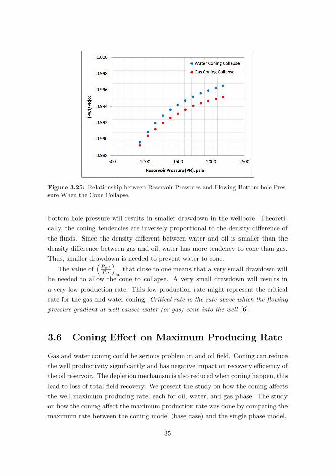
Figure 3.25: Relationship between Reservoir Pressures and Flowing Bottom-hole Pres-sure When the Cone Collapse.

bottom-hole pressure will results in smaller drawdown in the wellbore. Theoreti-

cally, the coning tendencies are inversely proportional to the density difference of

the fluids. Since the density different between water and oil is smaller than the

density difference between gas and oil, water has more tendency to cone than gas.

Thus, smaller drawdown is needed to prevent water to cone.

The value of(

Pwf

PR

)cc

that close to one means that a very small drawdown will

be needed to allow the cone to collapse. A very small drawdown will results in

a very low production rate. This low production rate might represent the critical

rate for the gas and water coning. Critical rate is the rate above which the flowing

pressure gradient at well causes water (or gas) cone into the well [6].

3.6 Coning Effect on Maximum Producing Rate

Gas and water coning could be serious problem in and oil field. Coning can reduce

the well productivity significantly and has negative impact on recovery efficiency of

the oil reservoir. The depletion mechanism is also reduced when coning happen, this

lead to loss of total field recovery. We present the study on how the coning affects

the well maximum producing rate; each for oil, water, and gas phase. The study

on how the coning affect the maximum production rate was done by comparing the

maximum rate between the coning model (base case) and the single phase model.

35

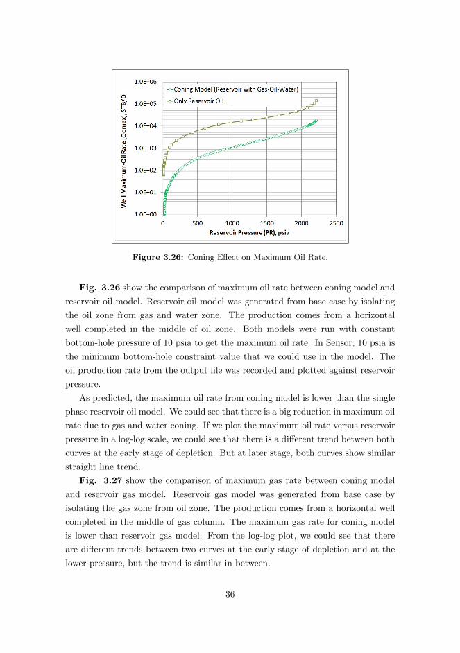
Figure 3.26: Coning Effect on Maximum Oil Rate.

Fig. 3.26 show the comparison of maximum oil rate between coning model and

reservoir oil model. Reservoir oil model was generated from base case by isolating

the oil zone from gas and water zone. The production comes from a horizontal

well completed in the middle of oil zone. Both models were run with constant

bottom-hole pressure of 10 psia to get the maximum oil rate. In Sensor, 10 psia is

the minimum bottom-hole constraint value that we could use in the model. The

oil production rate from the output file was recorded and plotted against reservoir

pressure.

As predicted, the maximum oil rate from coning model is lower than the single

phase reservoir oil model. We could see that there is a big reduction in maximum oil

rate due to gas and water coning. If we plot the maximum oil rate versus reservoir

pressure in a log-log scale, we could see that there is a different trend between both

curves at the early stage of depletion. But at later stage, both curves show similar

straight line trend.

Fig. 3.27 show the comparison of maximum gas rate between coning model

and reservoir gas model. Reservoir gas model was generated from base case by

isolating the gas zone from oil zone. The production comes from a horizontal well

completed in the middle of gas column. The maximum gas rate for coning model

is lower than reservoir gas model. From the log-log plot, we could see that there

are different trends between two curves at the early stage of depletion and at the

lower pressure, but the trend is similar in between.

36

Figure 3.27: Coning Effect on Maximum Gas Rate.

Figure 3.28: Coning Effect on Maximum Water Rate.

Fig. 3.28 show the comparison of maximum water rate between coning model

and reservoir water model. Reservoir water model was generated from base case by

isolating the water zone from oil zone. The production comes from one horizontal

well completed in the middle of water column. The maximum water rate from

reservoir water is higher than the coning model. From the log-log plot, we could

see that there is different trend between two curves at early stage of depletion, but

37

in general, both have similar profile of maximum rate versus reservoir pressure.

Based on this study, we could conclude that the maximum rate at coning condition

is lower than the maximum rate at condition where production comes from single

phase reservoir. The presences of other fluids in production stream that create a

flow resistant is part of the reason. In coning model, where simultaneous gas and

water coning occurs in thin oil reservoir, the maximum rate for each phase most

likely depend on mobility, effective permeability, fluid density, gas cap size, aquifer

size, and oil zone thickness.

38

Chapter 4

IPR MODELING FOR

HORIZONTAL WELL

WITH CONING

4.1 Introduction

Inflow Performance Relationship (IPR) is the relationship of well flowing bottom-

hole pressure (BHP) with well flow rate (q) at stabilized reservoir pressure. In

many applications, IPR is used in production optimization. For examples; to de-

termine tubing and choke size, adequate design of artificial lift, optimum well rate,

production forecast, etc.

In 1935, Rawlins and Schellhardt [27] first present the concept of IPR by plotting

the effect of liquid loading on production performance. Gilbert [15] is the first one

who utilized curved which related flow rate with pressure and introduced them

as IPR curves. In 1968, Vogel generated IPR curves for several hypothetical oil

reservoirs with variety of PVT properties and relative permeability data by using

a computer model. He also generated a dimensionless IPR for these set of IPR

and proposed a relationship between the dimensionless parameters [31]. Since

then, numbers of various correlations for IPR calculation have been proposed in

literature.

Examples of IPR equations for horizontal well could be found in [9, 10, 17, 19,

20, 35]. The productivity equations can also be used to generate IPR. References 8,

39

23, and 27 present the productivity equations for horizontal well. These equations

require several reservoir properties in its calculation (e.g permeability, reservoir

thickness, etc).

In this study, based on the work of Vogel, we generated the IPR curves and

its dimensionless form at any stage of depletion using Sensor black-oil simulator

results. The IPR was generated for horizontal well with gas and water coning prob-

lems, producing from thin oil reservoir sandwiched between gas cap and aquifer.

The IPR equation based on SPE paper by Whitson [33] that best-fit the gas, oil,

water IPR is also presented in this study.

The empirical IPR generated with several major simplifying assumptions as

follow: (1) The porous medium with areal permeability isotropy and vertical

anisotropy; (2) Zero capillary pressure; (3) Skin effect is neglected; (4) Negligi-

ble frictional losses in horizontal wellbore; (5) The well is fully penetrating the

reservoir in horizontal direction; (6) Reservoir model is run with initial pressure

equal to bubble point.

4.2 Dimensional IPR Curves

Dimensional IPR curve was generated from pairs of flowing bottom-hole pressure

and production rate at constant reservoir pressure. To represent the stage of de-

pletion; instead of using recovery factor, we use reservoir pressure as a fraction of

initial reservoir pressure. Since we modeled a three-phase reservoir, there will be

an IPR curve each for gas, oil, and water phase.

The base case model was run with constant flowing bottom-hole pressure using

Sensor simulator. The gas, oil, and water production rate and reservoir pressure

from the output file were tabulated in an excel worksheet for further data process-

ing. Repetition of the same procedure with different flowing bottom-hole pressure

constraint was done to obtain more IPR data. An example of tabulated IPR data

from the output file before sorting is shown in Table 4.1.

Since IPR curve is generated at constant reservoir pressure while the data are

tabulated for each flowing bottom-hole pressure, a look-up and interpolation pro-

cedures in Excel are needed to get flowing bottom-hole and production data tab-

ulated for constant reservoir pressure. The following is the excel function used to

do interpolation and look-up [4]:

=FORECAST(NewX, OFFSET(KnownY, MATCH(NewX, KnownX, 1)

– 1, 0, 2), OFFSET(KnownX, MATCH(NewX, KnownX, 1) – 1, 0, 2)

40

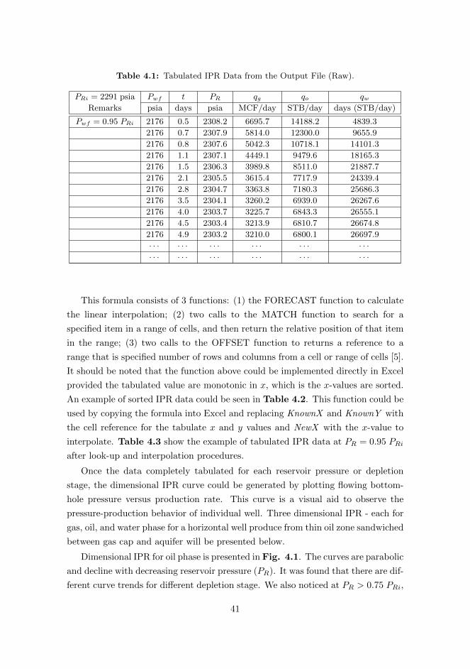
Table 4.1: Tabulated IPR Data from the Output File (Raw).

PRi = 2291 psia Pwf t PR qg qo qwRemarks psia days psia MCF/day STB/day days (STB/day)

Pwf = 0.95 PRi 2176 0.5 2308.2 6695.7 14188.2 4839.3

2176 0.7 2307.9 5814.0 12300.0 9655.9

2176 0.8 2307.6 5042.3 10718.1 14101.3

2176 1.1 2307.1 4449.1 9479.6 18165.3

2176 1.5 2306.3 3989.8 8511.0 21887.7

2176 2.1 2305.5 3615.4 7717.9 24339.4

2176 2.8 2304.7 3363.8 7180.3 25686.3

2176 3.5 2304.1 3260.2 6939.0 26267.6

2176 4.0 2303.7 3225.7 6843.3 26555.1

2176 4.5 2303.4 3213.9 6810.7 26674.8

2176 4.9 2303.2 3210.0 6800.1 26697.9

· · · · · · · · · · · · · · · · · ·· · · · · · · · · · · · · · · · · ·

This formula consists of 3 functions: (1) the FORECAST function to calculate

the linear interpolation; (2) two calls to the MATCH function to search for a

specified item in a range of cells, and then return the relative position of that item

in the range; (3) two calls to the OFFSET function to returns a reference to a

range that is specified number of rows and columns from a cell or range of cells [5].

It should be noted that the function above could be implemented directly in Excel

provided the tabulated value are monotonic in x, which is the x-values are sorted.

An example of sorted IPR data could be seen in Table 4.2. This function could be

used by copying the formula into Excel and replacing KnownX and KnownY with

the cell reference for the tabulate x and y values and NewX with the x-value to

interpolate. Table 4.3 show the example of tabulated IPR data at PR = 0.95 PRi

after look-up and interpolation procedures.

Once the data completely tabulated for each reservoir pressure or depletion

stage, the dimensional IPR curve could be generated by plotting flowing bottom-

hole pressure versus production rate. This curve is a visual aid to observe the

pressure-production behavior of individual well. Three dimensional IPR - each for

gas, oil, and water phase for a horizontal well produce from thin oil zone sandwiched

between gas cap and aquifer will be presented below.

Dimensional IPR for oil phase is presented in Fig. 4.1. The curves are parabolic

and decline with decreasing reservoir pressure (PR). It was found that there are dif-

ferent curve trends for different depletion stage. We also noticed at PR > 0.75 PRi,

41

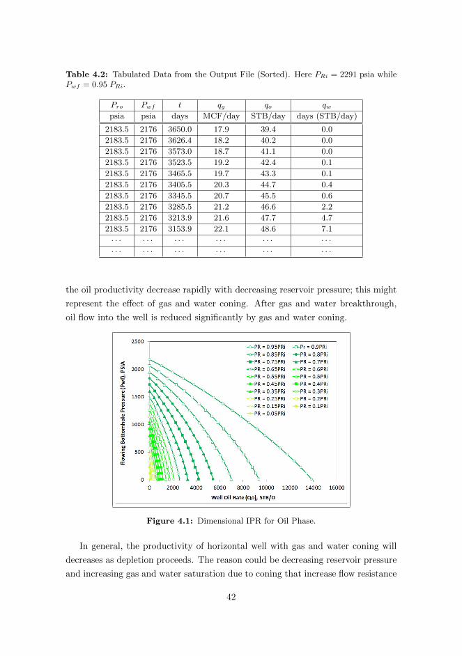
Table 4.2: Tabulated Data from the Output File (Sorted). Here PRi = 2291 psia whilePwf = 0.95 PRi.

Pro Pwf t qg qo qwpsia psia days MCF/day STB/day days (STB/day)

2183.5 2176 3650.0 17.9 39.4 0.0

2183.5 2176 3626.4 18.2 40.2 0.0

2183.5 2176 3573.0 18.7 41.1 0.0

2183.5 2176 3523.5 19.2 42.4 0.1

2183.5 2176 3465.5 19.7 43.3 0.1

2183.5 2176 3405.5 20.3 44.7 0.4

2183.5 2176 3345.5 20.7 45.5 0.6

2183.5 2176 3285.5 21.2 46.6 2.2

2183.5 2176 3213.9 21.6 47.7 4.7

2183.5 2176 3153.9 22.1 48.6 7.1

· · · · · · · · · · · · · · · · · ·· · · · · · · · · · · · · · · · · ·

the oil productivity decrease rapidly with decreasing reservoir pressure; this might

represent the effect of gas and water coning. After gas and water breakthrough,

oil flow into the well is reduced significantly by gas and water coning.

Figure 4.1: Dimensional IPR for Oil Phase.

In general, the productivity of horizontal well with gas and water coning will

decreases as depletion proceeds. The reason could be decreasing reservoir pressure

and increasing gas and water saturation due to coning that increase flow resistance

42

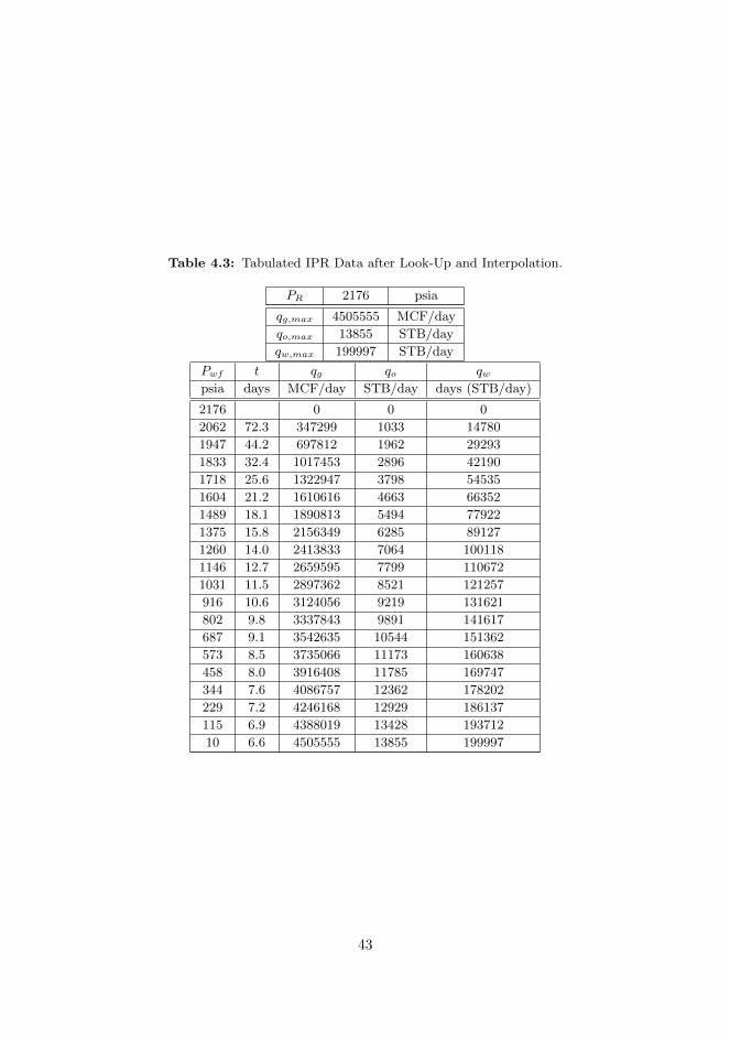
Table 4.3: Tabulated IPR Data after Look-Up and Interpolation.

PR 2176 psia

qg,max 4505555 MCF/day

qo,max 13855 STB/day

qw,max 199997 STB/day

Pwf t qg qo qwpsia days MCF/day STB/day days (STB/day)

2176 0 0 0

2062 72.3 347299 1033 14780

1947 44.2 697812 1962 29293

1833 32.4 1017453 2896 42190

1718 25.6 1322947 3798 54535

1604 21.2 1610616 4663 66352

1489 18.1 1890813 5494 77922

1375 15.8 2156349 6285 89127

1260 14.0 2413833 7064 100118

1146 12.7 2659595 7799 110672

1031 11.5 2897362 8521 121257

916 10.6 3124056 9219 131621

802 9.8 3337843 9891 141617

687 9.1 3542635 10544 151362

573 8.5 3735066 11173 160638

458 8.0 3916408 11785 169747

344 7.6 4086757 12362 178202

229 7.2 4246168 12929 186137

115 6.9 4388019 13428 193712

10 6.6 4505555 13855 199997

43

to oil. For a constant flowing bottom-hole pressure (Pwf ), there will be higher oil

rate in high-pressure reservoir compare to low-pressure reservoir (Fig. 4.1). This

primarily because higher reservoir pressure will result in higher well-drawdown for

a constant Pwf ; theoretically, oil rate is proportional with well-drawdown.

Figure 4.2: Dimensional IPR for Gas Phase.

Fig. 4.2 show the dimensional IPR for gas phase. This is the visual represen-

tation of pressure-gas production behavior of a horizontal well from the base case

model. The gas production (well gas rate) mainly comes from the coning free-gas

from gas cap; only relatively small fraction of production comes from the solution

gas. As shown in Fig. 4.2, the IPR curves also have a curvature shape with quite

similar trends when reservoir pressure goes below 0.85 PRi.

Different curves characteristic was found at early stage of depletion, when PR ≥0.85 PRi. For detail observation, only three IPR curves at early stage of depletion

were plot in Fig. 4.3. These curves might represent the gas coning development

at early stage of depletion. When the well start producing above the critical rate,

where the well drawdown causes viscous forces overcome the gravity forces, gas

coning from gas cap will occurs. With decreasing reservoir pressure, the gas cap

starts to expand and push the oil column down to the water zone (Fig. 2.5). This

cause the gas-oil contact move closer to perforation point and results in severe

gas coning where more gas produce in production stream. In this situation, as

we observed in Fig. 4.3, the gas rate might increase with decreasing reservoir

pressure.

44

Figure 4.3: Dimensional IPR for Gas Phase (Early stage of depletion).

Figure 4.4: Dimensional IPR for Water Phase.

Dimensional IPR for water phase is presented in Fig. 4.4. This plot represents

the pressure-water production behavior of horizontal well producing under three-

phase flow condition. It should be noted that the water production comes from

aquifer-water that cone into the well when the rate higher than critical rate.

The IPR curves are parabolic and decline with decreasing reservoir pressure

(PR). In general, the productivity will decreases as depletion proceeds. But refer

45

to Fig. 4.4, we observed that the water productivity decease quite rapid when

the reservoir pressure goes from 0.95 PRi to 0.85 PRi, the curves trends are then

similar until 0.5 PRi and somewhat slightly differ when reservoir pressure goes be-

low 0.5 PRi. This curves characteristic might be caused by gas and water coning

dynamic in reservoir. When the reservoir pressure decrease at early stage of de-

pletion; gas cap start to expand and push the oil column to the water zone, the

gas coning also start to build and dominate the flow in production stream. The

combination of these event cause a higher resistance to water to flow and results

in quite rapid decrease of water productivity at early stage.

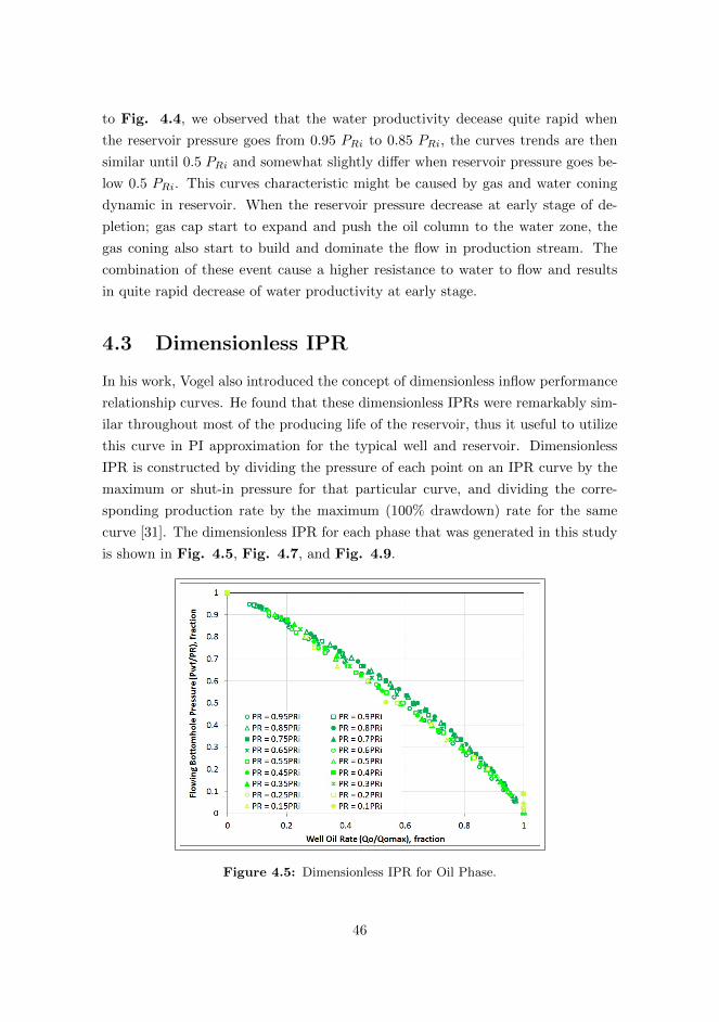
4.3 Dimensionless IPR

In his work, Vogel also introduced the concept of dimensionless inflow performance

relationship curves. He found that these dimensionless IPRs were remarkably sim-

ilar throughout most of the producing life of the reservoir, thus it useful to utilize

this curve in PI approximation for the typical well and reservoir. Dimensionless

IPR is constructed by dividing the pressure of each point on an IPR curve by the

maximum or shut-in pressure for that particular curve, and dividing the corre-

sponding production rate by the maximum (100% drawdown) rate for the same

curve [31]. The dimensionless IPR for each phase that was generated in this study

is shown in Fig. 4.5, Fig. 4.7, and Fig. 4.9.

Figure 4.5: Dimensionless IPR for Oil Phase.

46

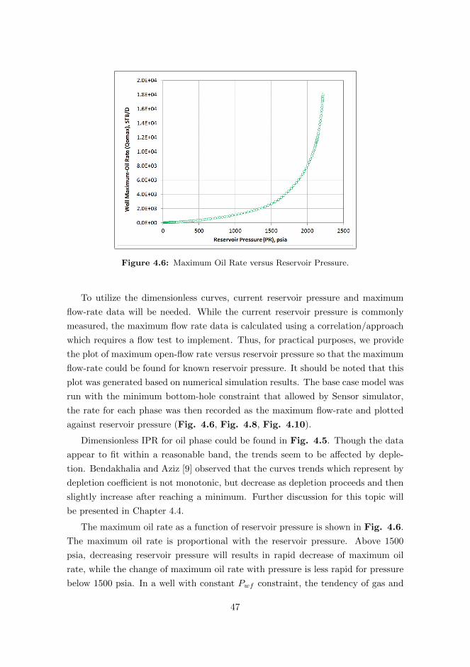
Figure 4.6: Maximum Oil Rate versus Reservoir Pressure.

To utilize the dimensionless curves, current reservoir pressure and maximum

flow-rate data will be needed. While the current reservoir pressure is commonly

measured, the maximum flow rate data is calculated using a correlation/approach

which requires a flow test to implement. Thus, for practical purposes, we provide

the plot of maximum open-flow rate versus reservoir pressure so that the maximum

flow-rate could be found for known reservoir pressure. It should be noted that this

plot was generated based on numerical simulation results. The base case model was

run with the minimum bottom-hole constraint that allowed by Sensor simulator,

the rate for each phase was then recorded as the maximum flow-rate and plotted

against reservoir pressure (Fig. 4.6, Fig. 4.8, Fig. 4.10).

Dimensionless IPR for oil phase could be found in Fig. 4.5. Though the data

appear to fit within a reasonable band, the trends seem to be affected by deple-

tion. Bendakhalia and Aziz [9] observed that the curves trends which represent by

depletion coefficient is not monotonic, but decrease as depletion proceeds and then

slightly increase after reaching a minimum. Further discussion for this topic will

be presented in Chapter 4.4.

The maximum oil rate as a function of reservoir pressure is shown in Fig. 4.6.

The maximum oil rate is proportional with the reservoir pressure. Above 1500

psia, decreasing reservoir pressure will results in rapid decrease of maximum oil

rate, while the change of maximum oil rate with pressure is less rapid for pressure

below 1500 psia. In a well with constant Pwf constraint, the tendency of gas and

47

water coning is greater at high reservoir pressure (high drawdown) and lower at

low reservoir pressure (low drawdown).

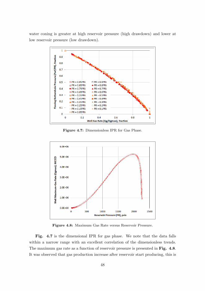
Figure 4.7: Dimensionless IPR for Gas Phase.

Figure 4.8: Maximum Gas Rate versus Reservoir Pressure.

Fig. 4.7 is the dimensional IPR for gas phase. We note that the data falls

within a narrow range with an excellent correlation of the dimensionless trends.

The maximum gas rate as a function of reservoir pressure is presented in Fig. 4.8.

It was observed that gas production increase after reservoir start producing, this is

48

due to gas coning that occurs when dynamic force greater than gravitational force.

But as depletion proceeds and a lower drawdown exist, the gas coning tendency

and production rate is lower.

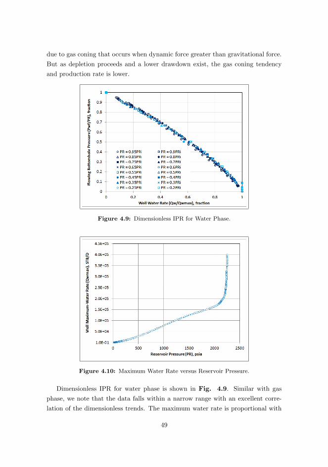
Figure 4.9: Dimensionless IPR for Water Phase.

Figure 4.10: Maximum Water Rate versus Reservoir Pressure.

Dimensionless IPR for water phase is shown in Fig. 4.9. Similar with gas

phase, we note that the data falls within a narrow range with an excellent corre-

lation of the dimensionless trends. The maximum water rate is proportional with

49

reservoir pressure (Fig. 4.10). Since the well completed 5 ft from WOC, early

water coning occurs when reservoir start producing. But as gas production from

coning increase and dominate the flow, water production rate decrease rapidly. As

depletion proceeds and the lower drawdown exist, the tendency of water coning

and production rate is lower. Though the dimensionless IPR for gas and water

phase appear to be independent from depletion stage, two generalized IPRs will

still developed in this study for application purposes. The first empirical IPR will

be developed as a function of reservoir pressure or depletion stage while the second

empirical IPR will be developed based on all the generated data.

4.4 IPR Equation to Best-Fit Gas, Oil, and Water

Phases

The formulation to best-fit the dimensionless IPR will be taken from IPR model

presented by Whitson in SPE paper 12518 [33]. Whitson proposed a simple ap-

proach for OIL reservoir based on Fetkovich [14] suggestion that F (P ) for oil sys-

tem can be approximated by two straight line joined at bubble point. Using the

linear relationship of F (P ) as suggested by Fetkovich, Whitson defined the ex-

pression for dimensionless pseudo-pressure, md, for completely saturated system

(Pwf ≤ PR ≤ Pb) as:

md = 1 − V

(Pwf

PR

)− (1 − V )

(Pwf

PR

)2

(4.1)

Where

V =2x

(x+ 1)(4.2)

Since we are using the assumption of negligible High Velocity Fluid (HVF) effect:

md =q

qmax(4.3)

Hence, (4.1) becomes:

q

qmax= 1 − V

(Pwf

PR

)− (1 − V )

(Pwf

PR

)2

(4.4)

50

The formulation given by (4.4) will be used to best-fit the IPR models for gas,

oil, and water phase in this study. This formulation is similar with the general IPR

model proposed by Richardson and Shaw for solution gas reservoirs [28].

4.4.1 Depletion based IPR

Since the pressure-production rate behavior of a horizontal well appears to be

affected by depletion [9], an empirical IPR was developed based on simulated data

on each reservoir pressure (stage of depletion). The equations used to best-fit the

IPR model for each phase are:

Oil phase :qo

qo,max= 1 − Vo

(Pwf

PR

)− (1 − Vo)

(Pwf

PR

)2

(4.5)

Gas phase :qg

qg,max= 1 − Vg

(Pwf

PR

)− (1 − Vg)

(Pwf

PR

)2

(4.6)

Water phase :qw

qw,max= 1 − Vw

(Pwf

PR

)− (1 − Vw)

(Pwf

PR

)2

(4.7)

Where Vo, Vg, and Vw is the parameter in general quadratic equation for oil,

gas, and water. Bendakhalia and Aziz observed that V is a function of reservoir

recovery or depletion, thus they defined V as the depletion coefficient.

The following are procedures to calculate Vo, Vg, and Vw at each reservoir

pressure:

1. Assume Vo, Vg, and Vw value as initial guess. The value should between 0

and 1.

2. Calculate Pwf/PR for each data point.

3. For each phase, calculate the analytical qqmax

by using (4.5)-(4.7).

4. Calculate the error square between numerical and analytical qqmax

using equa-

tion below

q

qmax=

[(q/qmax)analytical − (q/qmax)numerical

(q/qmax)numerical

]2(4.8)

51

5. Calculate the Sum of Square Error for gas, oil, and water (SSQg,SSQo, and

SSQw)

6. Calculate the Total SSQ;

Total SSQ = SSQg + SSQo + SSQw (4.9)

7. Utilize SOLVER in MS Excel to minimize the Total SSQ by changing Vo, Vg,

and Vw values.

The procedures above were repeated for all reservoir pressure. Fig. 4.11

presents the Vo and SSQo values for the ranges of reservoir pressure studied. The

SSQo was also plotted to observe how fit the data with the IPR model.

Figure 4.11: Vo and SSQo as a Function of Reservoir Pressure.

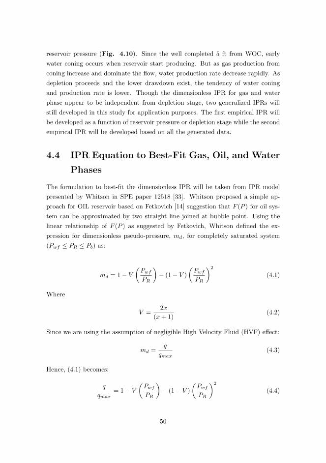
From Fig. 4.11, we note that Vo, or depletion coefficient for oil phase as

defined by Bendakhalia and Aziz, is not monotonic. The SSQo curve is higher

at reservoir pressure between 750 – 1500 psia, this indicate an increasing lack of

fit of the data on this region. We would comment that the Vo points in higher

SSQo region are located out of the trend, thus it is possible that these data points

actually following the trend of other data points. It appears that Vo decreases

with decreasing reservoir pressure and then increase after some point. Similar

observation of depletion coefficient for oil phase was made by Bendakhalia-Aziz

([9]) and Wiggins-Wang ([35]).

52

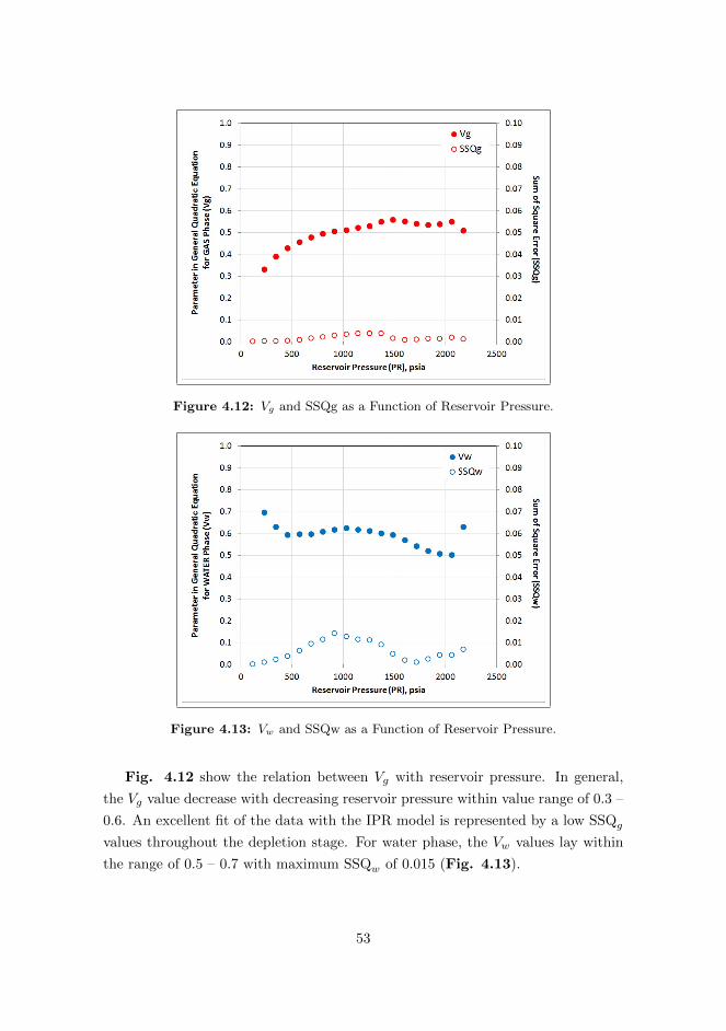
Figure 4.12: Vg and SSQg as a Function of Reservoir Pressure.

Figure 4.13: Vw and SSQw as a Function of Reservoir Pressure.

Fig. 4.12 show the relation between Vg with reservoir pressure. In general,

the Vg value decrease with decreasing reservoir pressure within value range of 0.3 –

0.6. An excellent fit of the data with the IPR model is represented by a low SSQg

values throughout the depletion stage. For water phase, the Vw values lay within

the range of 0.5 – 0.7 with maximum SSQw of 0.015 (Fig. 4.13).

53

Table 4.4: Summary of V and SSQ Values for Generalized IPR.

Parameter in General Quadratic Equation Value SSQ Value

Vo 0.522 SSQo 0.565

Vg 0.526 SSQg 0.063

Vw 0.576 SSQw 0.189

Compare to oil phase, the empirical IPR show a better fit for gas and water

phase. Thus, a better estimate of gas and water performance should be expected in

its application. We also noted that the depletion coefficient (V ) is not monotonic,

and there are different trends of depletion coefficient for each phase. This non-

monotonic behavior might indicate that the IPR is independent (or only a weak

function) of depletion stage. It should be noted that further studies will be needed

to validate this conclusion.

4.4.2 Generalized IPR

The second empirical IPR for each phase was developed based on all generated

data. Considering that the data appear to fit within reasonable band and there

is an indication that the IPR is independent of depletion, the generalized IPR

might accurate enough to estimate the three-phase inflow performance of horizontal

well produce from thin oil column sandwiched between gas cap and aquifer. This

suggestion is supported by Wiggins and Wang observation that the depletion based

IPR provide no better results than the generalized IPR.

The generalized IPR was developed using the same procedures as depletion

based IPR. But instead of calculating the SSQ for each reservoir pressure, the SSQ

was calculated for all data. Thus there are only three V values for all data, each for

gas, oil, and water phase. Table 4.4 presents the V and SSQ values for generalized

IPR.

As shown in Table 4.4; the calculation of Vg, Vo, and Vw results in approxi-

mately the same value of 0.5. Though this value might changes for different reser-

voir properties, it could not be overemphasize that Vg, Vo, and Vw values will

approximately the same. Thus, it is possible to use one generalized IPR for gas,

oil, and water phases with reasonable accuracy. Using (4.4) and the V values ob-

tained in this study, the resulting generalized IPR for each phase could be wrote

as follow:

54

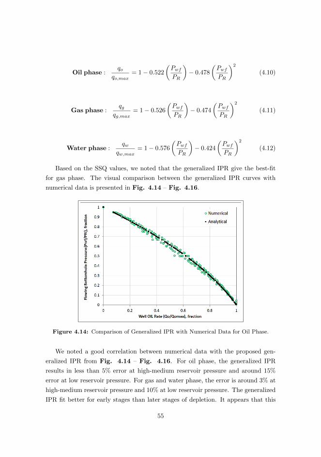
Oil phase :qo

qo,max= 1 − 0.522

(Pwf

PR

)− 0.478

(Pwf

PR

)2

(4.10)

Gas phase :qg

qg,max= 1 − 0.526

(Pwf

PR

)− 0.474

(Pwf

PR

)2

(4.11)

Water phase :qw

qw,max= 1 − 0.576

(Pwf

PR

)− 0.424

(Pwf

PR

)2

(4.12)

Based on the SSQ values, we noted that the generalized IPR give the best-fit

for gas phase. The visual comparison between the generalized IPR curves with

numerical data is presented in Fig. 4.14 – Fig. 4.16.

Figure 4.14: Comparison of Generalized IPR with Numerical Data for Oil Phase.

We noted a good correlation between numerical data with the proposed gen-

eralized IPR from Fig. 4.14 – Fig. 4.16. For oil phase, the generalized IPR

results in less than 5% error at high-medium reservoir pressure and around 15%

error at low reservoir pressure. For gas and water phase, the error is around 3% at

high-medium reservoir pressure and 10% at low reservoir pressure. The generalized

IPR fit better for early stages than later stages of depletion. It appears that this

55

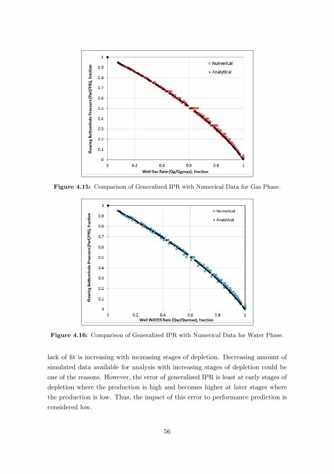
Figure 4.15: Comparison of Generalized IPR with Numerical Data for Gas Phase.

Figure 4.16: Comparison of Generalized IPR with Numerical Data for Water Phase.

lack of fit is increasing with increasing stages of depletion. Decreasing amount of

simulated data available for analysis with increasing stages of depletion could be

one of the reasons. However, the error of generalized IPR is least at early stages of

depletion where the production is high and becomes higher at later stages where

the production is low. Thus, the impact of this error to performance prediction is

considered low.

56

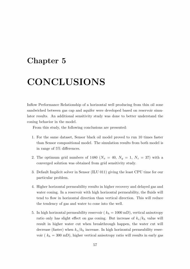
Chapter 5

CONCLUSIONS

Inflow Performance Relationship of a horizontal well producing from thin oil zone

sandwiched between gas cap and aquifer were developed based on reservoir simu-

lator results. An additional sensitivity study was done to better understand the

coning behavior in the model.

From this study, the following conclusions are presented:

1. For the same dataset, Sensor black oil model proved to run 10 times faster

than Sensor compositional model. The simulation results from both model is

in range of 5% differences.

2. The optimum grid numbers of 1480 (Nx = 40, Ny = 1, Nz = 37) with a

converged solution was obtained from grid sensitivity study.

3. Default Implicit solver in Sensor (ILU 011) giving the least CPU time for our

particular problem.

4. Higher horizontal permeability results in higher recovery and delayed gas and

water coning. In a reservoir with high horizontal permeability, the fluids will

tend to flow in horizontal direction than vertical direction. This will reduce

the tendency of gas and water to cone into the well.

5. In high horizontal permeability reservoir ( kh = 1000 mD), vertical anisotropy

ratio only has slight effect on gas coning. But increase of kv/kh value will

result in higher water cut when breakthrough happen, the water cut will

decrease (faster) when kv/kh increase. In high horizontal permeability reser-

voir ( kh = 300 mD), higher vertical anisotropy ratio will results in early gas

57

breakthrough but slower increase of GOR; vertical anisotropy ratio only has

slight effect on water coning.

6. Gas cap size does not affect the water and gas breakthrough time, but trends

of GOR and water cut after breakthrough is affected by gas cap size. Bigger

gas cap size results in higher GOR but lower water cut. Increase in gas cap

size will results in lower oil recovery factor.

7. Aquifer size does not affect the gas and water breakthrough time. Increase

in aquifer size will leads to higher water cut and lower GOR. There is only

slight effect of aquifer size on oil recovery; with tripled aquifer volume, the

oil recovery increase less than 1%.

8. The trends of oil recovery with different well depth are changes with time;

in a long production period, it appears to be beneficial to place horizontal

well in upper section of the oil leg. It is recommended to generate the plot

of oil recovery versus well depth based on particular reservoir, development

plan, and well configuration data; and use it as a tool to help in deciding the

optimum well placement.

9. When the horizontal well completed below WOC, ’inverse coning’ of oil to the

well will happen in early period. But when the gas pushes oil column to the

water zone, the well actually produces from an oil column with gas and water

coning. So the inverse coning contributes in oil recovery at early period, but

the oil recovery at later stage relies on gas from gas cap that pushes the oil

into water zone.

10. A relationship curve between reservoir pressures and flowing bottom-hole

pressure when the cone collapse was presented in this study. The ratio of

bottom-hole pressure to reservoir pressure at which the cone starts to collapse

is higher for water coning than gas coning. This means, compare to gas cone

collapse, higher bottom-hole pressure will be needed to make the water cone

collapse.

11. The maximum rate at coning condition is lower than the maximum rate at

condition where production comes from single phase reservoir.

12. Three dimensional IPR for our particular model - each for gas, oil, and water

phase were generated in this study. These curves could help in observing

58

the pressure-production behavior of individual well. In general, the produc-

tivity of horizontal well with gas and water coning will decreases as depletion

proceeds.

13. Dimensionless IPR and maximum rate as a function of reservoir pressure for

each phase is presented in this study. We noted that the data falls within a

narrow range with an excellent correlation of the dimensionless trends.

14. Two empirical IPR, depletion based IPR and generalized IPR, were developed

based on formulation given by Whitson.

15. From depletion based IPRs, we observed that the depletion coefficient (V )

is not monotonic, and there are different trends of depletion coefficient for

each phase. The non-monotonic behavior might indicate that the IPR is

independent (or only a week function) of depletion stage.

16. Calculation of Vg, Vo, and Vw for the generalized IPR results in approximately

the same value of 0.5. Though this value might changes for different reservoir

properties, we suggest that the Vg, Vo, and Vw values will approximately the

same.

59

60

Nomenclatures

Bg = gas formation volume factor

Bo = oil formation volume factor

Nx = number of grids in x-direction

Ny = number of grids in y-direction

Nz = number of grids in z-direction

NZTOP = number of cells in z-direction; above the well

NZBOTTOM = number of cells in z-direction; below the well

Pwf = flowing bottom-hole pressure, bara or psia

PR = reservoir pressure, bara or psia

q = production rate, STB/D

qmax = maximum production rate, STB/D

Rx = ∆xi+1/∆xi

Rz = ∆zi+1/∆zi

SSQo = Sum of Square of Error for oil phase

SSQg = Sum of Square of Error for gas phase

SSQw = Sum of Square of Error for water phase

Vo = parameter in general quadratic IPR equation for oil phase

Vg = parameter in general quadratic IPR equation for gas phase

Vw = parameter in general quadratic IPR equation for water phase

∆x = grid size in block-i

∆y = grid size in block-j

∆z = grid size in block-k

61

62

Bibliography

[1] http://www.coatsengineering.com

[2] http://petrostreamz.com/pipe-it

[3] Sensor Manual

[4] http://www.blueleafsoftware.com/Products/Dagra/LinearInterpolationExcel.php

[5] Excel Help and How-to

[6] Ahmad, T., Reservoir Engineering Handbook Third Edition, Gulf Professional

Publishing, 2006.

[7] Appleyard, J. R. and Cheshire, I. M., Nested Factorization, SPE 12264 pre-

sented at the 7th SPE Symposium on Reservoir Simulation in San Francisco

(November 1983).

[8] Babu, D. K. and Odeh, A. S., Productivity of a Horizontal Well, SPE Paper

18298 presented at the 1988 SPE Ann. Tech. Conf. and Exhibition Houston.

[9] Bendakhlia, H. and Aziz, K., Inflow Performance Relationships for Solution

Gas Drive Horizontal Wells, SPE Paper 19823 presented at 64th SPE Annual

Technical Conference and Exhibition, San Antonio Texas (October 1989).

[10] Billiter, T., Lee, J., Chase, R., Dimensionless Inflow-Performance-Relationship

Curve for Unfractured Horizontal Gas Well, SPE Paper 72361 presented at

SPE Eastern Regional Meeting, Canton Ohio (October 2001).

[11] Daviau, F. et al., Pressure Analysis for Horizontal Wells, SPE 14251 presented

at SPE Annual Technical Conference and Exhibition, Las Vegas (September

1985).

63

[12] Eickmeier, J. R., How to Accurately Predict Future Well Productivities, World

Oil (May 1968).

[13] Elgaghah, S. A. et al., A Simple Productivity Equation for Horizontal Wells

Based on Drainage Area Concept, SPE 35713 presented at Western Regional

Meeting in Alaska (May 1996).

[14] Fetkovich, M. K., The Isochronal Testing of Oil Wells, SPE Paper 529 pre-

sented at SPE Annual Meeting, Las Vegas (September 1973).

[15] Gilbert, W. E., Flowing and Gas Lift Well Performance, API Drilling and

Production Practice, 1954, Dallas-Texas.

[16] Haug, B. T., Ferguson, W.I., Kydland, T., Horizontal Well in the Water Zone:

The Most Effective Way for Tapping Oil from Oil Zones?, SPE 22929 presented

at 66th Annual Technical Conference and Exhibition, Dallas Texas (October

1991).

[17] Huang, B. et al., A New IPRs Establishment and Solution for Horizontal

Wells, SPE Paper 39570 presented at SPE India Oil and Gas Conference and

Exhibition, New Delhi India (February 1998).

[18] Ibelegbu, C., Determination of Cone Receding Time in Horizontal Well, SPE

140684 presented at the 34th Annual SPE International Conference and Ex-

hibition, Tinapa Nigeria (August 2010).

[19] Jabbari, H. and Economides, M. J., A New Approach to IPR Curves of Hori-

zontal Wells in Two-Phase Reservoirs, SPE 115918 presented at SPE Annual

Technical Conference and Exhibition, Colorado USA (September 2008).

[20] Kamkom, R. and Zhu, D., Evaluation of Two-Phase IPR Correlations for Hor-

izontal Wells, SPE Paper 93986 presented at SPE Production and Operations

Symposium, Oklahoma USA (April 2005).

[21] Karcher, B. J., Giger, F. M., and Combe, J., Some Practical Formulas to

Predict Horizontal Wells Behavior, SPE Paper 15430 presented at the 1986

SPE Ann. Tech. Conf. and Exhibition New Orleans.

[22] Lee, R. L., et al., Water Cone Subsidence Time of a Horizontal Well, SPE

29295 presented at SPE Asia Pacific Oil and gas Conference, Kuala Lumpur

Malaysia (March 1995).

64

[23] Mukherjee, H. and Economides, M. J., A Parametric Comparison of Horizontal

and Vertical Well Performance, SPE Paper 18303 presented at the 1989 SPE

Ann. Tech. Conf. and Exhibition San Antonio.

[24] Ozkan, E., Raghavan, R., and Joshi, S. D., Horizontal Well Pressure Analysis,

SPEFE (December 1989).

[25] Papatzacos, P. et al. Cone Breakthrough Time for Horizontal Wells, SPE 19822

presented at the 64th SPE Annual Technical Conference and Exhibition, San

Antonio-Texas (October 1989).

[26] Price, H. S. and Coats, K. H., Direct Methods in Reservoir Simulation, SPEJ,

June 1974, Trans. AIME 257.

[27] Rawlins, E. L. and Schellhardt, M. A., Backpressure Data on Natural Gas

Wells and Their Application to Production Practices, Monograph Series,

USBM (1935).

[28] Richardson, J. M. and Shaw, A. H., Two-Rate IPR Testing a Practical Pro-

duction Tool, JCPT (March April 1982).

[29] Uhri, D. C., and Blount, E. M., Pivot Point Method Quickly Predicts Well

Performance, World Oil (May 1982).

[30] Vinsome, P. K. W., Orthomin, an Iterative Method for Solving Sparse Sets of

Simultaneous Linear Equations, SPE 5729 presented at the SPE 4th Sympo-

sium of Numerical Reservoir Simulation in Los Angeles (February 1976).

[31] Vogel, J. V., Inflow Performance Relationships for Solution-Gas Drive Wells,

JPT, January 1968

[32] Wagenhofer, T., and Hatzignatiou, D., G., Optimization of Horizontal Well

Placement, SPE 35714 presented at Western Regional Meeting, Anchorage

Alaska (May 1996).

[33] Whitson, C. H., Reservoir Well Performance and Predicting Deliverability,

SPE Paper 12518 (1983).

[34] Whitson, C.H. and Torp, S.B. ,Evaluating Constant Volume Depletion Data,

JPT, March 1983; Trans., AIME, 275.

65

[35] Wiggins, M. L. and Wang, H. S., A Two-Phase IPR for Horizontal Oil Wells,

SPE 94302 presented at SPE Production and Operations Symposium, Okla-

homa USA (April 2005).

66

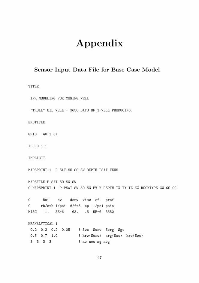
Appendix

Sensor Input Data File for Base Case Model

TITLE

IPR MODELING FOR CONING WELL

"TROLL" OIL WELL - 3650 DAYS OF 1-WELL PRODUCING.

ENDTITLE

GRID 40 1 37

ILU 0 1 1

IMPLICIT

MAPSPRINT 1 P SAT SO SG SW DEPTH PSAT TENS

MAPSFILE P SAT SO SG SW

C MAPSPRINT 1 P PSAT SW SO SG PV H DEPTH TX TY TZ KZ ROCKTYPE GW GO GG

C Bwi cw denw visw cf pref

C rb/stb 1/psi #/ft3 cp 1/psi psia

MISC 1. 3E-6 63. .5 5E-6 3550

KRANALYTICAL 1

0.2 0.2 0.2 0.05 ! Swc Sorw Sorg Sgc

0.5 0.7 1.0 ! krw(Sorw) krg(Swc) kro(Swc)

3 3 3 3 ! nw now ng nog

67

C ---------------------------------------------------------------------

C Grid dimensions - generated from Grid Builder Excel Sheet

C ---------------------------------------------------------------------

INCLUDE

DELX.inc

INCLUDE

DELY.inc

INCLUDE

DELZ.inc

C ---------------------------------------------------------------------

POROS CON

.25

MOD

1 40 1 1 1 1 = 100 ! BIG GAS CAP

1 40 1 1 37 37 = 100 ! BIG AQUIFER

DEPTH CON

5000

KX CON

1000

KY EQUALS KX

KZ EQUALS KX

MOD

1 40 1 1 1 37 * 0.25

C ---------------------------------------------------------------------

C Automatic conversion of EOS to Black Oil Table

C ---------------------------------------------------------------------

68

C ipvttype nsat ntot

BLACKOIL 1 15 15

PRESSURES 14.7 100 250 500 750 1000 1250 1500 1750 2000 2100 2291 2500

2750 3000

RESERVOIR FLUID

0.00371018 0.40442424 0.04443788 0.01973696 0.22678725 0.20551770

0.07982091 0.01556488

INJECTION GAS EQUILIBRIUM

SEPARATOR

14.7 60.

ENDBLACKOIL

C Include EOS

INCLUDE

eos8x-viso14.inc

C ---------------------------------------------------------------------

INITIAL

C depth psat

DEPTH PSATBP

5050. 2291.

C PINIT 2291 - DO NOT enter PINIT if GOC is entered

GOC 5050

HWC 5100

ENDINIT

WELL

I J K

PROD1

1 -1 26

69

WELLTYPE

PROD1 RBTOT

BHP

PROD1 1500

MAPSFREQ 1

MAPSFILEFREQ 1

RATE

PROD1 10000

TIME 7300 365

END

70