Www.sti-innsbruck.at © Copyright 2008 STI INNSBRUCK Lecture IV – xx 2009 Theorem Proving, Logic...
68
www.sti-innsbruck.at © Copyright 2008 STI INNSBRUCK www.sti- innsbruck.at Lecture IV – xx 2009 Theorem Proving, Logic Programming, and Description Logics Dieter Fensel and Florian Fischer Intelligent Systems
-
Upload
avis-kelly -
Category
Documents
-
view
213 -
download
0
Transcript of Www.sti-innsbruck.at © Copyright 2008 STI INNSBRUCK Lecture IV – xx 2009 Theorem Proving, Logic...

www.sti-innsbruck.at © Copyright 2008 STI INNSBRUCK www.sti-innsbruck.at
Lecture IV – xx 2009Theorem Proving, Logic Programming, and Description Logics
Dieter Fensel and Florian Fischer
Intelligent Systems
www.sti-innsbruck.at 2
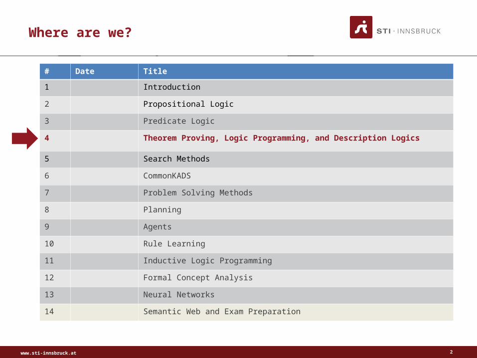
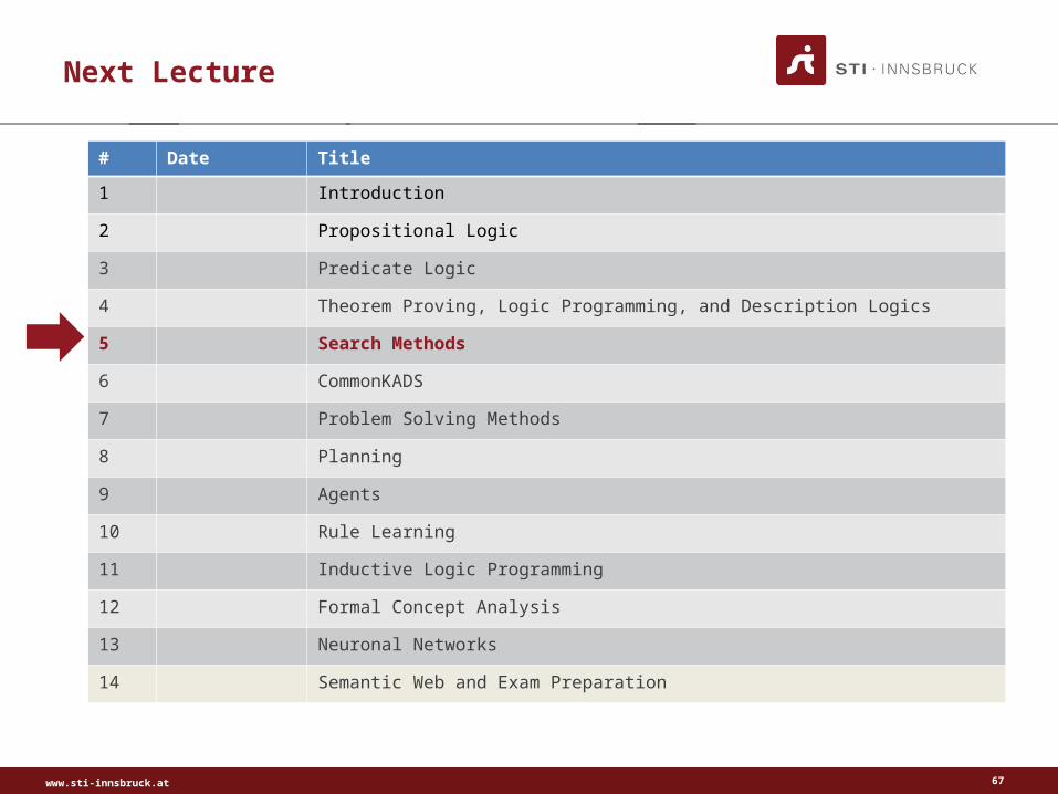
# Date Title
1 Introduction
2 Propositional Logic
3 Predicate Logic
4 Theorem Proving, Logic Programming, and Description Logics
5 Search Methods
6 CommonKADS
7 Problem Solving Methods
8 Planning
9 Agents
10 Rule Learning
11 Inductive Logic Programming
12 Formal Concept Analysis
13 Neural Networks
14 Semantic Web and Exam Preparation
Where are we?
www.sti-innsbruck.at
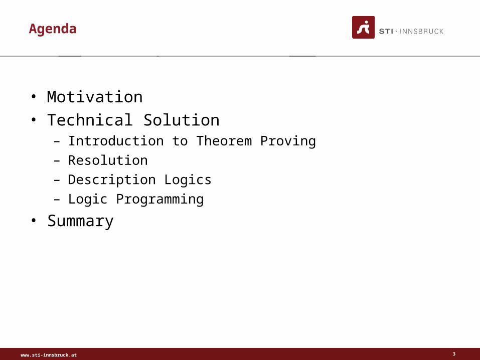
Agenda
• Motivation• Technical Solution
– Introduction to Theorem Proving– Resolution– Description Logics– Logic Programming
• Summary
3

www.sti-innsbruck.at
MOTIVATION
4

www.sti-innsbruck.at
Motivation
• Basic results of mathematical logic show:– We can do logical reasoning with a limited set of simple
(computable) rules in restricted formal languages like First-order Logic (FOL)
– Computers can do reasoning
• FOL is interesting for this purpose because:– It is expressive enough to capture many foundational theorems
of mathematics (i.e. Set Theory, Peano Arithmetic, ...)– Many real-world problems can be formalized in FOL– It is the most expressive logic that one can adequately approach
with automated theorem proving techniques– Subsets of it can be used for more specialized applications
5
www.sti-innsbruck.at
TECHNICAL SOLUTIONSTheorem Proving, Description Logics, and Logic Programming
6

www.sti-innsbruck.at
THEOREM PROVING
7

www.sti-innsbruck.at
Modelling(automated)
Deduction
Introduction - Logic and Theorem Proving
Real-world descriptionin natural language.Mathematical ProblemsProgram + Specification
Syntax (formal language).First-order Logic, Dynamic Logic, …
Valid Formulae
Provable Formulae
Formalization
Semantics(truth function)
Calculus(derivation / proof)
Correctness
Completeness
Diagram by Uwe Keller
www.sti-innsbruck.at
Introduction – Logic and Theorem Proving
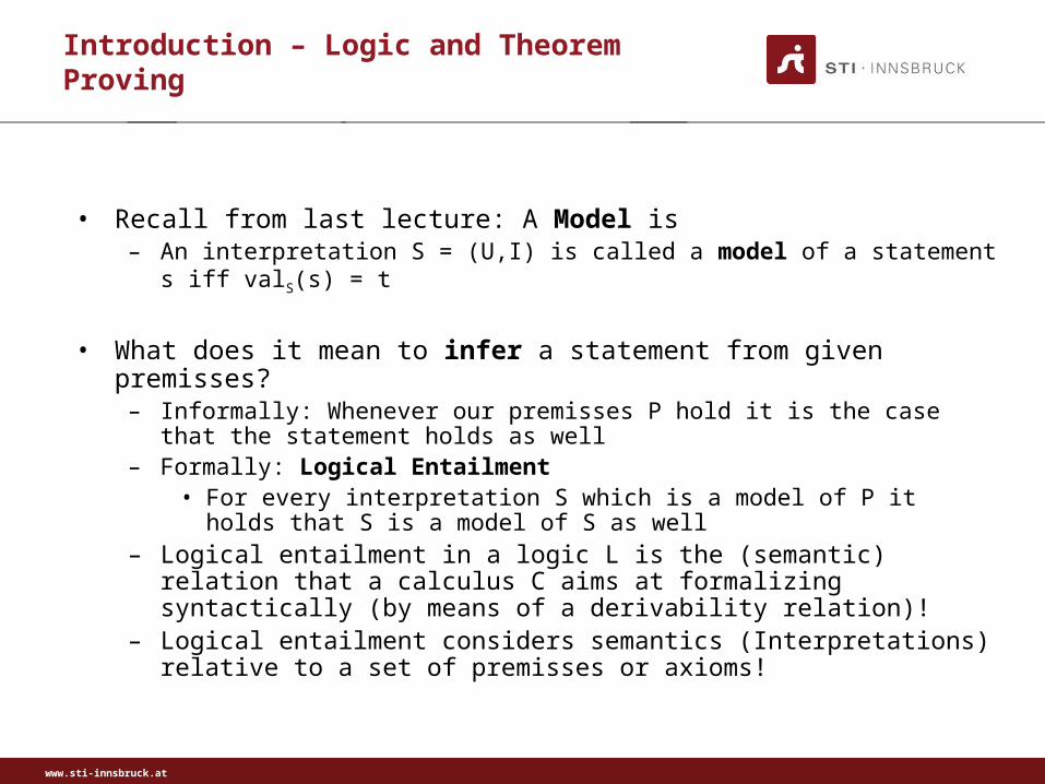
• Recall from last lecture: A Model is– An interpretation S = (U,I) is called a model of a statement s iff valS(s) = t
• What does it mean to infer a statement from given premisses?– Informally: Whenever our premisses P hold it is the case that the statement holds
as well– Formally: Logical Entailment
• For every interpretation S which is a model of P it holds that S is a model of S as well
– Logical entailment in a logic L is the (semantic) relation that a calculus C aims at formalizing syntactically (by means of a derivability relation)!
– Logical entailment considers semantics (Interpretations) relative to a set of premisses or axioms!
www.sti-innsbruck.at
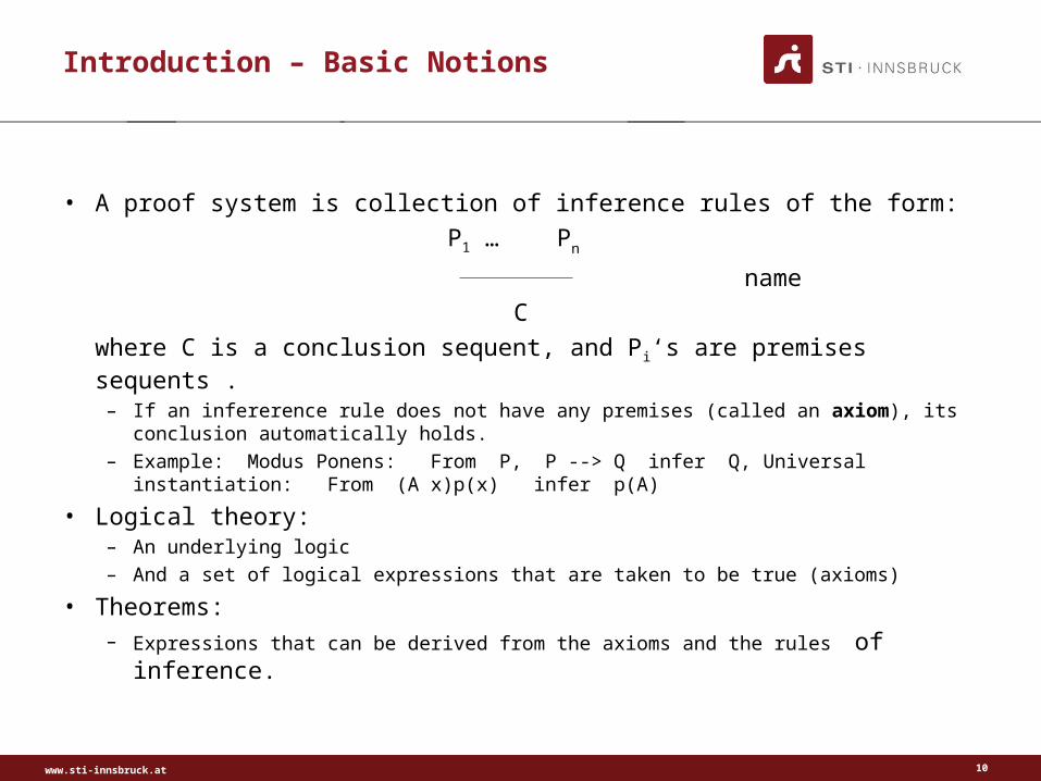
Introduction – Basic Notions
• A proof system is collection of inference rules of the form:
P1 … Pn
name
C
where C is a conclusion sequent, and Pi‘s are premises sequents . – If an infererence rule does not have any premises (called an axiom), its conclusion
automatically holds.– Example: Modus Ponens: From P, P --> Q infer Q, Universal instantiation:
From (A x)p(x) infer p(A)
• Logical theory: – An underlying logic– And a set of logical expressions that are taken to be true (axioms)
• Theorems:– Expressions that can be derived from the axioms and the rules of inference.
10
www.sti-innsbruck.at
Introduction – Basic Notions
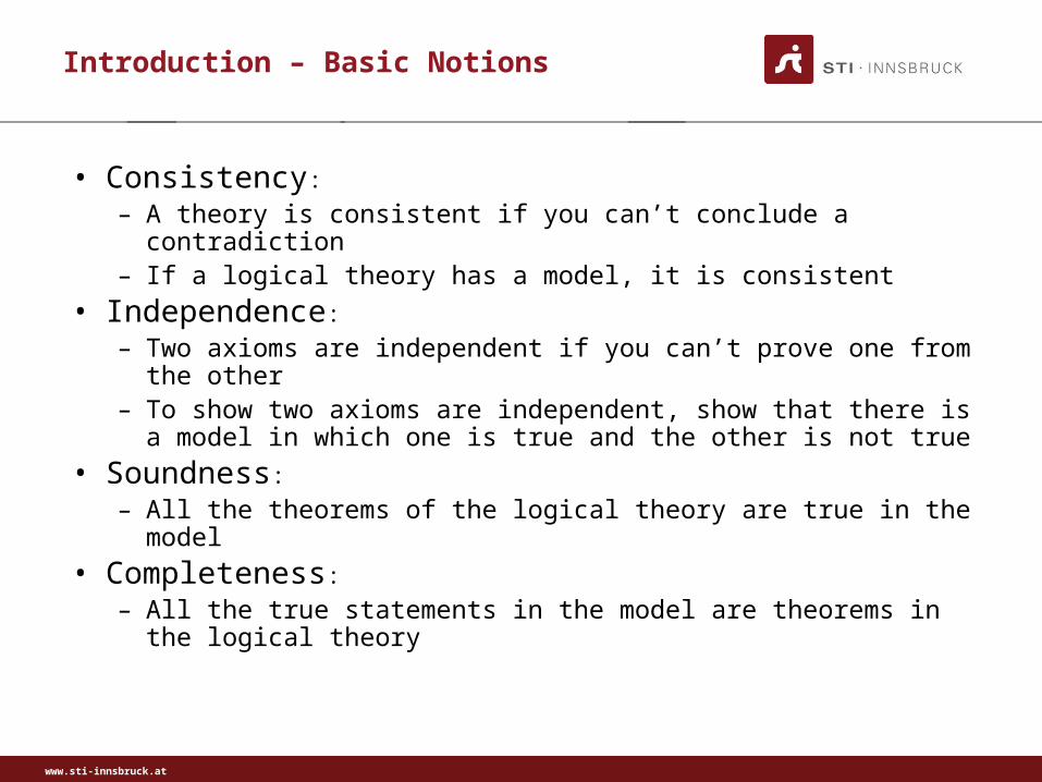
• Consistency:
– A theory is consistent if you can’t conclude a contradiction– If a logical theory has a model, it is consistent
• Independence:
– Two axioms are independent if you can’t prove one from the other
– To show two axioms are independent, show that there is a model in which one is true and the other is not true
• Soundness:
– All the theorems of the logical theory are true in the model
• Completeness:
– All the true statements in the model are theorems in the logical theory

www.sti-innsbruck.at Resolution Theorem Proving 12
Resolution - Principle
• Resolution refutation proves a theorem by: 1. Negating the statement to be proved
2. Adding this negated goal to the set of axioms that are known to be true.
3. Use the resolution rule of inference to show that this leads to a contradiction.→ Once the theorem prover shows that the negated goal is inconsistent with
the given set of axioms, it follows that the original goal must be consistent.
• Detailed steps in a resolution proof– Put the premises or axioms into clause normal form (CNF)– Add the negation of the to be proven statement, in clause form, to the set of
axioms– Resolve these clauses together, producing new clauses that logically follow
from them– Derive a contradiction by generating the empty clause.– The substitutions used to produce the empty clause are those under which
the opposite of the negated goal is true
www.sti-innsbruck.at
Normal Forms
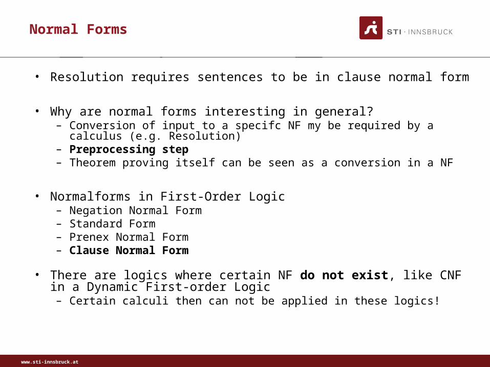
• Resolution requires sentences to be in clause normal form
• Why are normal forms interesting in general?– Conversion of input to a specifc NF my be required by a calculus (e.g.
Resolution) – Preprocessing step– Theorem proving itself can be seen as a conversion in a NF
• Normalforms in First-Order Logic– Negation Normal Form– Standard Form– Prenex Normal Form– Clause Normal Form
• There are logics where certain NF do not exist, like CNF in a Dynamic First-order Logic– Certain calculi then can not be applied in these logics!
www.sti-innsbruck.at Resolution Theorem Proving 14
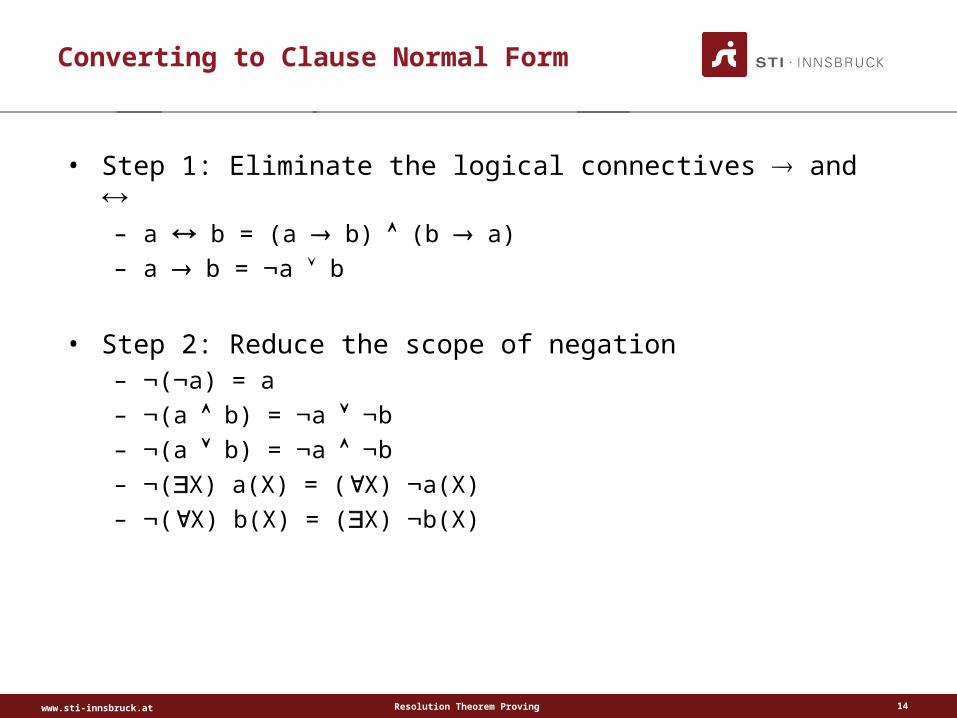
Converting to Clause Normal Form
• Step 1: Eliminate the logical connectives and – a b = (a b) (b a)
– a b = a b
• Step 2: Reduce the scope of negation– (a) = a
– (a b) = a b
– (a b) = a b
– (X) a(X) = (X) a(X)
– (X) b(X) = (X) b(X)

www.sti-innsbruck.at Resolution Theorem Proving 15
Converting to Clause Normal Form
• Step 3: Standardize by renaming all variables so that variables bound by different quantifiers have unique names
– (X) a(X) (X) b(X) = (X) a(X) (Y) b(Y)
• Step 4: Move all quantifiers to the left to obtain a prenex normal form
• Step 5: Eliminate existential quantifiers by using skolemization
www.sti-innsbruck.at Resolution Theorem Proving 16
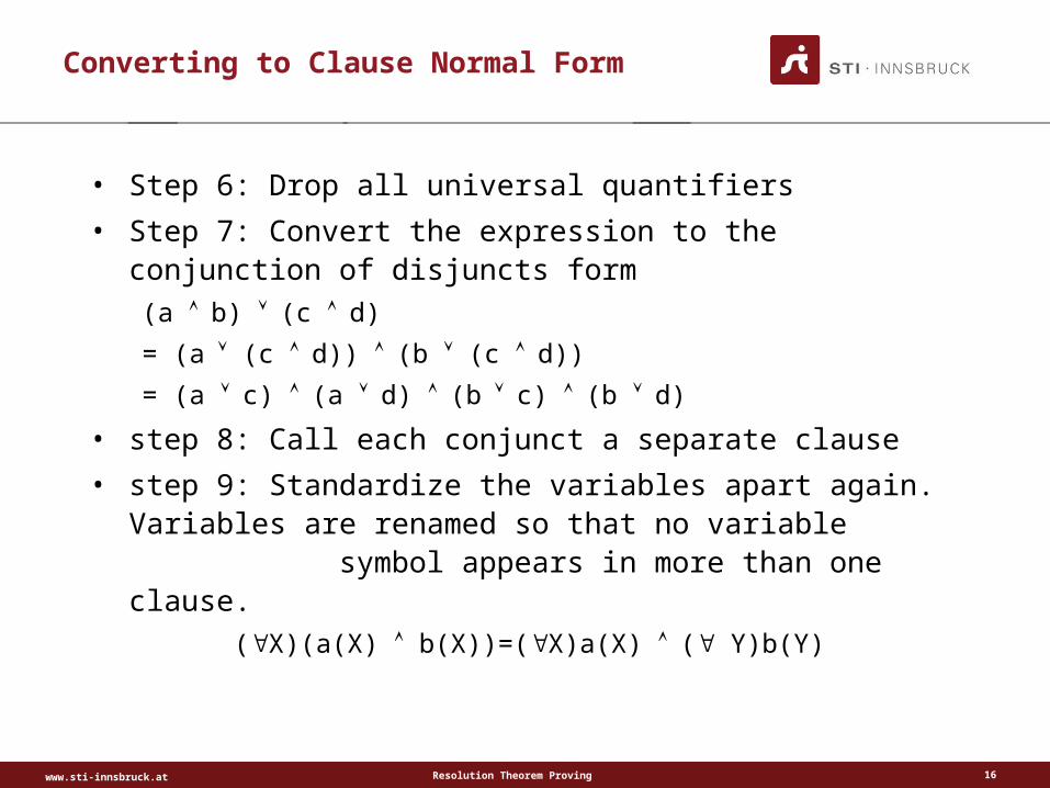
Converting to Clause Normal Form
• Step 6: Drop all universal quantifiers
• Step 7: Convert the expression to the conjunction of disjuncts form
(a b) (c d)
= (a (c d)) (b (c d))
= (a c) (a d) (bc) (b d)
• step 8: Call each conjunct a separate clause
• step 9: Standardize the variables apart again. Variables are renamed so that no variable symbol appears in more than one clause.
(X)(a(X) b(X))=(X)a(X) ( Y)b(Y)

www.sti-innsbruck.at Resolution Theorem Proving 17
Converting to Clause Normal Form
• Skolemization– Skolem constant
• (X)(dog(X)) may be replaced by dog(fido) where the name fido is picked from the domain of definition of X to represent that individual X.
– Skolem function
• If the predicate has more than one argument and the existentially quantified variable is within the scope of universally quantified variables, the existential variable must be a function of those other variables.
• (X)(Y)(mother(X,Y)) (X)mother(X,m(X))
• (X)(Y)(Z)(W)(foo (X,Y,Z,W))
(X)(Y)(W)(foo(X,Y,f(X,Y),w))

www.sti-innsbruck.at Resolution Theorem Proving 18
Converting to Clause Normal Form
• Example of Converting Clause Form
(X)([a(X) b(X)] [c(X,I) (Y)((Z)[C(Y,Z)] d(X,Y))]) ( X)(e(X))
– step 1: (X)([a(X) b(X)] [c(X,I) (Y)((Z)[c(Y,Z)] d(X,Y))]) (x)(e(X))
– step 2: (X)([a(X) b(X)] [c(X,I) (Y)((Z)[c(Y,Z)] d(X,Y))]) (x)(e(X))
– step 3: (X)([a(X) b(X)] [c(X,I) (Y)((Z)[c(Y,Z)] d(X,Y))]) (W)(e(W))
– step 4: (X)(Y)(Z)(W)([a(X) b(X)] [c(X,I) (c(Y,Z) d(X,Y))]) (e(W))
– step 5: (X)(Z)(W)([a(X) b(X)] [c(X,I) (c(f(X),Z) d(X,f(X)))]) (e(W))
– step 6: [a(X) b(X)] [c(X,I) (c(f(X),Z) d(X,f(X)))]) e(W)
www.sti-innsbruck.at Resolution Theorem Proving 19
Converting to Clause Normal Form
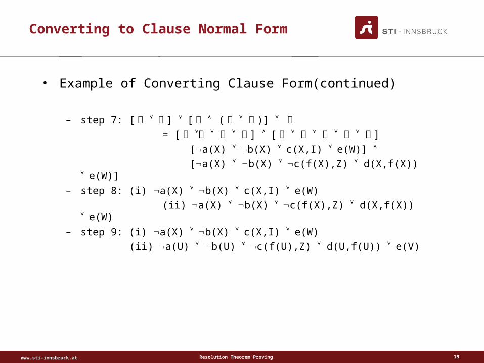
• Example of Converting Clause Form(continued)
– step 7: [ 가 나 ] [ 다 ( 라 마 )] 바 = [ 가 나 다 바 ] [ 가 나 라 마 바 ]
[a(X) b(X) c(X,I) e(W)] [a(X) b(X) c(f(X),Z) d(X,f(X)) e(W)]
– step 8: (i) a(X) b(X) c(X,I) e(W)
(ii)a(X) b(X) c(f(X),Z) d(X,f(X)) e(W)– step 9: (i) a(X) b(X) c(X,I) e(W)
(ii)a(U) b(U) c(f(U),Z) d(U,f(U)) e(V)
www.sti-innsbruck.at Resolution Theorem Proving 20
Resolution - Example
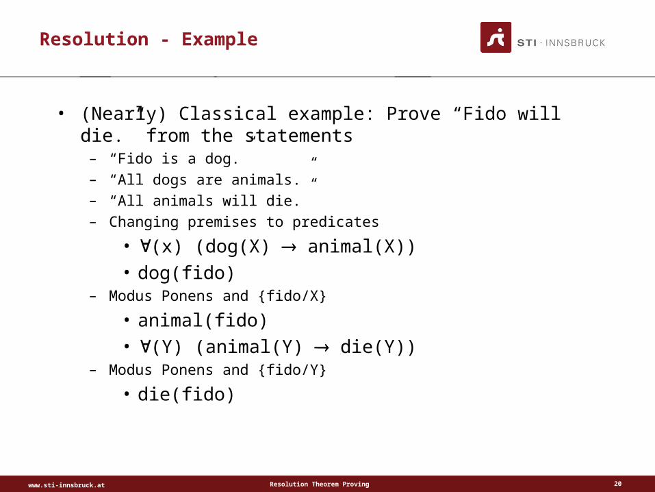
• (Nearly) Classical example: Prove “Fido will die.” from the statements
– “Fido is a dog.”– “All dogs are animals.” – “All animals will die.”– Changing premises to predicates
• (x) (dog(X) animal(X))• dog(fido)
– Modus Ponens and {fido/X}
• animal(fido)• (Y) (animal(Y) die(Y))
– Modus Ponens and {fido/Y}
• die(fido)
www.sti-innsbruck.at Resolution Theorem Proving 21
Resolution - Example
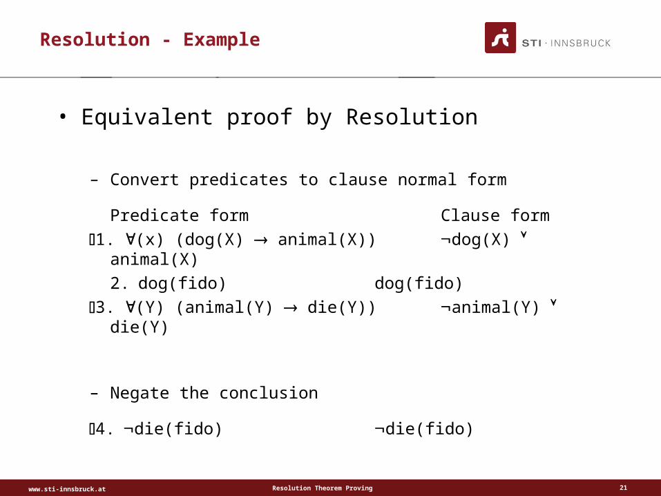
• Equivalent proof by Resolution
– Convert predicates to clause normal form
Predicate form Clause form
1.(x) (dog(X) animal(X))dog(X) animal(X)
2.dog(fido) dog(fido)
3.(Y) (animal(Y) die(Y)) animal(Y) die(Y)
– Negate the conclusion
4.die(fido) die(fido)
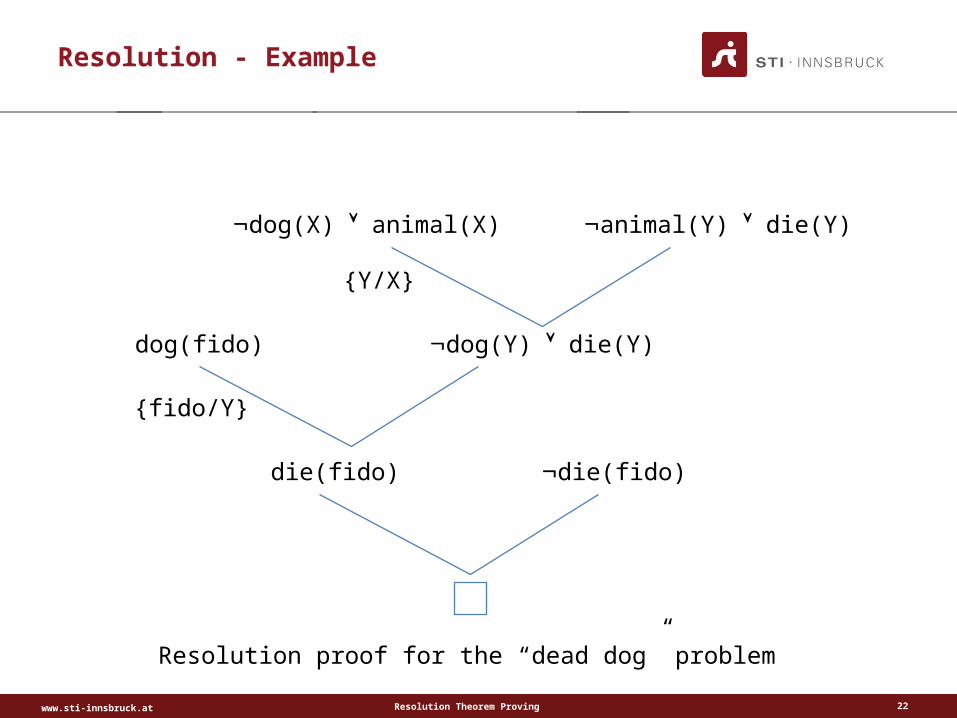
www.sti-innsbruck.at Resolution Theorem Proving 22
Resolution - Example
Resolution proof for the “dead dog” problem
dog(X) animal(X) animal(Y) die(Y)
dog(Y) die(Y)dog(fido)
die(fido) die(fido)
{Y/X}
{fido/Y}
www.sti-innsbruck.at Resolution Theorem Proving 23
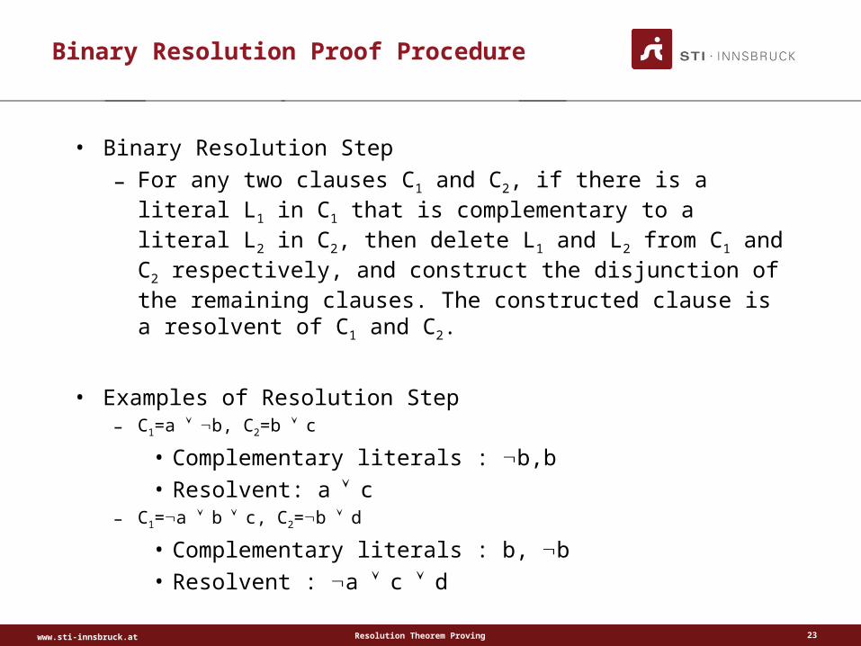
Binary Resolution Proof Procedure
• Binary Resolution Step
– For any two clauses C1 and C2, if there is a literal L1 in C1 that is complementary to a literal L2 in C2, then delete L1 and L2 from C1 and C2 respectively, and construct the disjunction of the remaining clauses. The constructed clause is a resolvent of C1 and C2.
• Examples of Resolution Step– C1=a b, C2=b c
• Complementary literals : b,b• Resolvent: ac
– C1=a bc, C2=b d
• Complementary literals : b, b• Resolvent : a c d
www.sti-innsbruck.at Resolution Theorem Proving 24
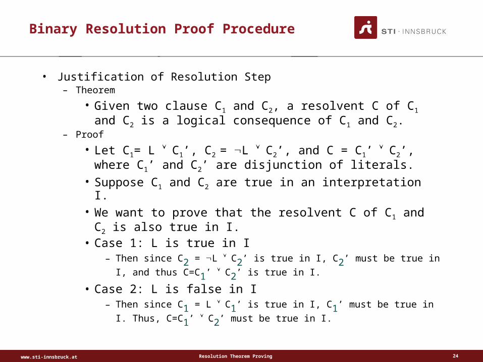
Binary Resolution Proof Procedure
• Justification of Resolution Step– Theorem
• Given two clause C1 and C2, a resolvent C of C1 and C2 is a logical consequence of C1 and C2.
– Proof
• Let C1= L C1’, C2 = L C2’, and C = C1’C2’, where C1’ and C2’ are disjunction of literals.
• Suppose C1 and C2 are true in an interpretation I.• We want to prove that the resolvent C of C1 and C2 is also
true in I.• Case 1: L is true in I
– Then since C2 = L C2’ is true in I, C2’ must be true in I, and thus
C=C1’ C2’ is true in I.
• Case 2: L is false in I– Then since C1 = L C1’ is true in I, C1’ must be true in I. Thus,
C=C1’ C2’ must be true in I.
www.sti-innsbruck.at Resolution Theorem Proving 25
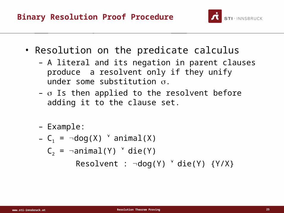
Binary Resolution Proof Procedure
• Resolution on the predicate calculus– A literal and its negation in parent clauses produce a
resolvent only if they unify under some substitution . – Is then applied to the resolvent before adding it to the
clause set.
– Example:
– C1 = dog(X) animal(X)
C2 = animal(Y) die(Y)
Resolvent : dog(Y) die(Y) {Y/X}

www.sti-innsbruck.at Resolution Theorem Proving 26
Strategies for Resolution
• Order of clause combination is important– N clauses N2 ways of combinations or checking to see whether
they can be combined
– Search heuristics are very important in resolution proof procedures
• Strategies– Breadth-First Strategy
– Set of Support Strategy
– Unit Preference Strategy
– Linear Input Form Strategy
www.sti-innsbruck.at
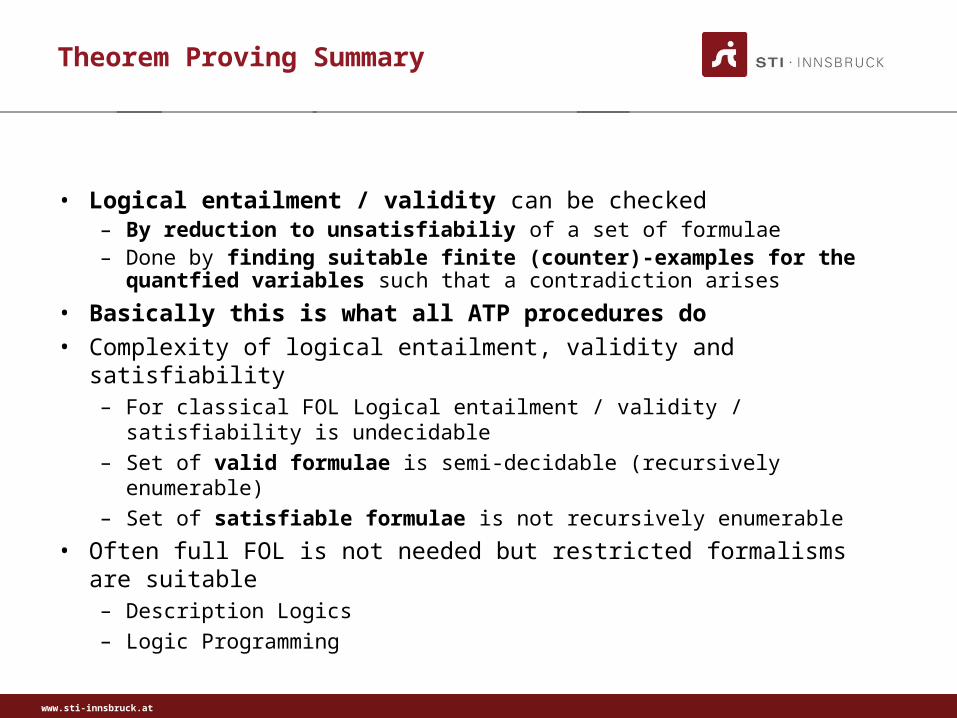
Theorem Proving Summary
• Logical entailment / validity can be checked– By reduction to unsatisfiabiliy of a set of formulae– Done by finding suitable finite (counter)-examples for the
quantfied variables such that a contradiction arises
• Basically this is what all ATP procedures do• Complexity of logical entailment, validity and satisfiability
– For classical FOL Logical entailment / validity / satisfiability is undecidable
– Set of valid formulae is semi-decidable (recursively enumerable)
– Set of satisfiable formulae is not recursively enumerable
• Often full FOL is not needed but restricted formalisms are suitable– Description Logics
– Logic Programming

www.sti-innsbruck.at
DESCRIPTION LOGICS
28

www.sti-innsbruck.at
Description Logic
• Most Description Logics are based on a 2-variable fragment of First Order Logic
– Classes (concepts) correspond to unary predicates– Properties correspond to binary predicates
• Restrictions in general:– Quantifiers range over no more than 2 variables– Transitive properties are an exception to this rule– No function symbols (decidability!)
• Most DLs are decidable and usually have decision procedures for key reasoning tasks
• DLs have more efficient decision problems than First Order Logic• We later show the very basic DL ALC as example
– More complex DLs work in the same basic way but have different expressivity
29

www.sti-innsbruck.at
Description Logic Basics
• Concepts/classes (unary predicates/formulae with one free variable)– E.g. Person, Female
• Roles (binary predicates/formulae with two free variables)– E.g. hasChild
• Individuals (constants)– E.g. Mary, John
• Constructors allow to form more complex concepts/roles– Union ⊔: Man ⊔ Woman– Intersection ⊓ : Doctor ⊓ Mother– Existential restriction ∃: ∃hasChild.Doctor (some child is a doctor)– Value(universal) restriction ∀: ∀hasChild.Doctor (all children are doctors)– Complement /negation¬: Man ⊑ ¬Mother– Number restriction ≥n, ≤n
• Axioms– Subsumption ⊑ : Motherr ⊑ Parent
30
www.sti-innsbruck.at
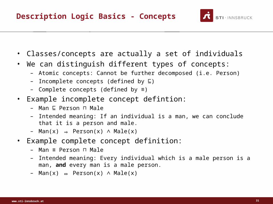
Description Logic Basics - Concepts
• Classes/concepts are actually a set of individuals• We can distinguish different types of concepts:
– Atomic concepts: Cannot be further decomposed (i.e. Person)– Incomplete concepts (defined by ⊑)– Complete concepts (defined by ≡)
• Example incomplete concept defintion:– Man ⊑ Person ⊓ Male– Intended meaning: If an individual is a man, we can conclude that it is a
person and male.– Man(x) ⇒ Person(x) ∧ Male(x)
• Example complete concept definition:– Man ≡ Person ⊓ Male– Intended meaning: Every individual which is a male person is a man, and
every man is a male person.– Man(x) ⇔ Person(x) ∧ Male(x)
31
www.sti-innsbruck.at
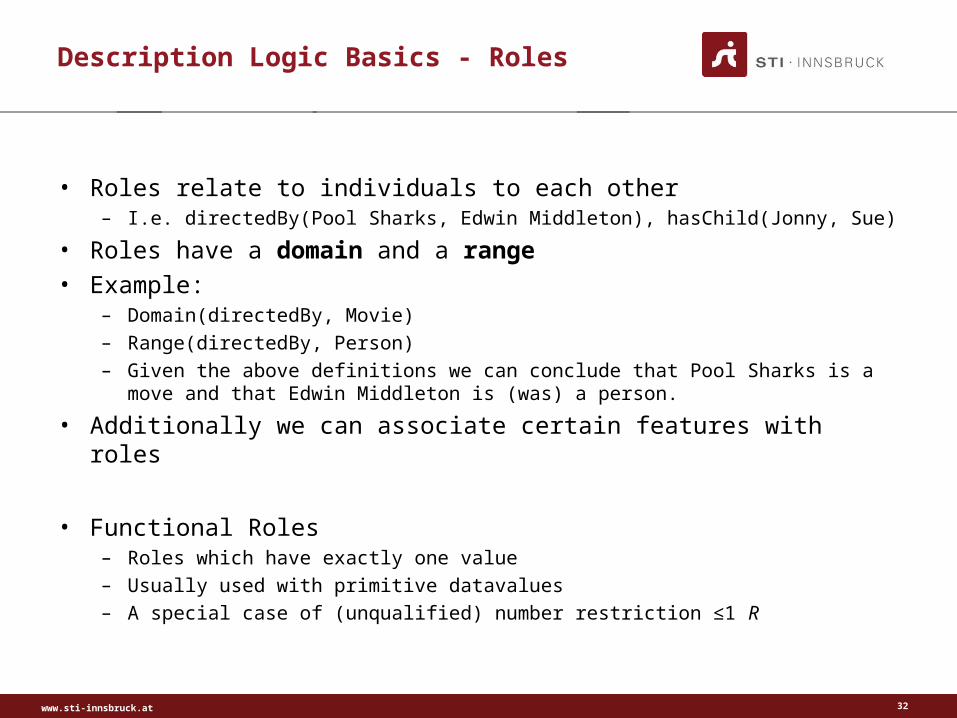
Description Logic Basics - Roles
• Roles relate to individuals to each other– I.e. directedBy(Pool Sharks, Edwin Middleton), hasChild(Jonny, Sue)
• Roles have a domain and a range• Example:
– Domain(directedBy, Movie)– Range(directedBy, Person)– Given the above definitions we can conclude that Pool Sharks is a move and that
Edwin Middleton is (was) a person.
• Additionally we can associate certain features with roles
• Functional Roles– Roles which have exactly one value– Usually used with primitive datavalues– A special case of (unqualified) number restriction ≤1 R
32
www.sti-innsbruck.at
Description Logic Basics - Roles
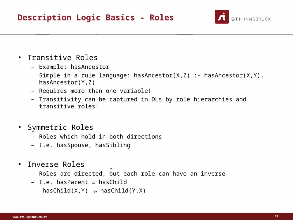
• Transitive Roles– Example: hasAncestor
Simple in a rule language: hasAncestor(X,Z) :- hasAncestor(X,Y), hasAncestor(Y,Z).
– Requires more than one variable!– Transitivity can be captured in DLs by role hierarchies and transitive roles:
• Symmetric Roles– Roles which hold in both directions– I.e. hasSpouse, hasSibling
• Inverse Roles– Roles are directed, but each role can have an inverse– I.e. hasParent ≡ hasChild
hasChild(X,Y) ⇔ hasChild(Y,X)
33

www.sti-innsbruck.at
Description Logic Knowledge Bases
• Typically a DL knowledge base (KB) consists of two components– Tbox (terminology): A set of inclusion/equivalence axioms denoting the
conceptual schema/vocabulary of a domain• Bear ⊑ Animal ⊓ Large• transitive(hasAncestor)• hasChild ≡ hasParent
– Abox (assertions): Axioms, which describe concrete instance data and holds assertions about individuals
• hasAncestor(Susan, Granny)• Bear(Winni Puh)
• From a theoretical point of view this division is arbitrary• But it is a useful simplification
34
www.sti-innsbruck.at
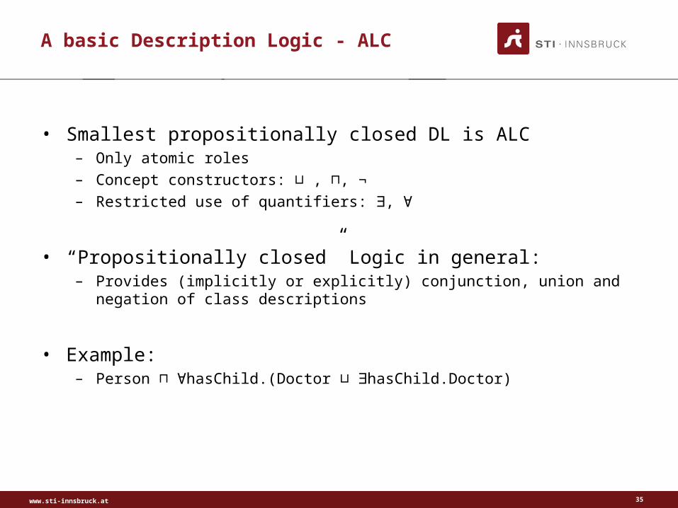
A basic Description Logic - ALC
• Smallest propositionally closed DL is ALC– Only atomic roles– Concept constructors: ⊔ , ⊓, ¬– Restricted use of quantifiers: ∃, ∀
• “Propositionally closed” Logic in general: – Provides (implicitly or explicitly) conjunction, union and negation of class
descriptions
• Example:– Person ⊓ ∀hasChild.(Doctor ⊔ ∃hasChild.Doctor)
35
www.sti-innsbruck.at
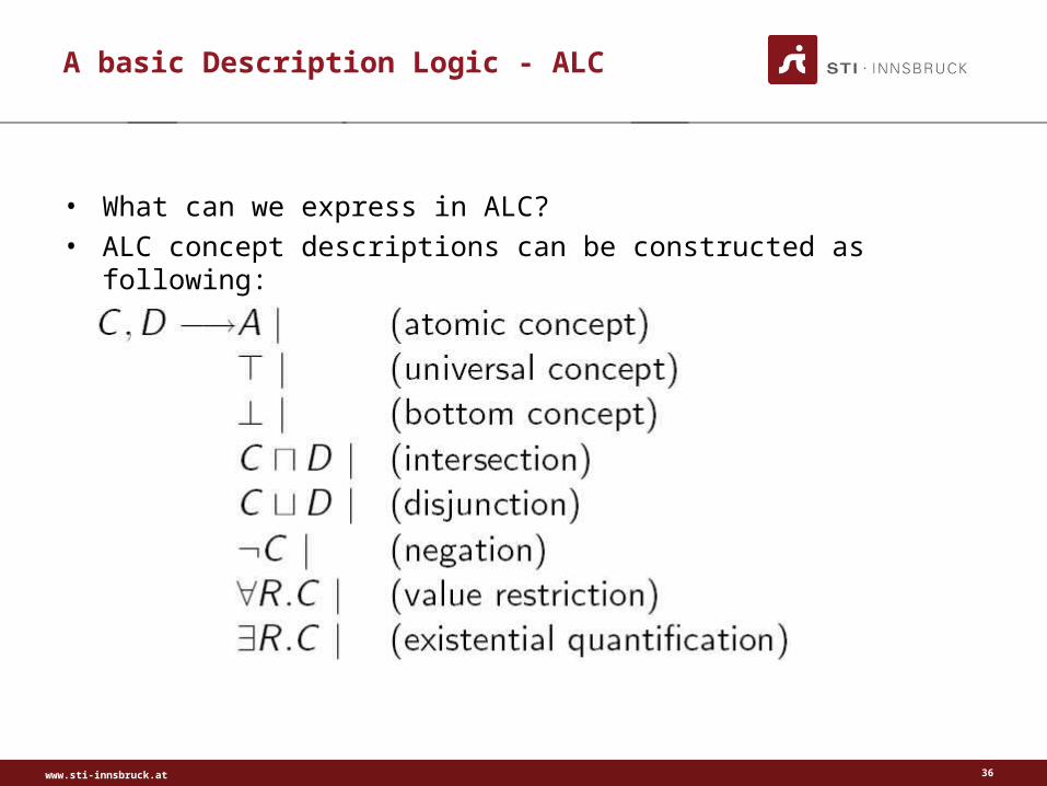
A basic Description Logic - ALC
• What can we express in ALC? • ALC concept descriptions can be constructed as following:
36

www.sti-innsbruck.at
A basic Description Logic - ALC
• Individual assertions :– a ∈ C– Mary is a Woman.
• Role assertions:– ⟨a, b ∈ R⟩– E.g. Marry loves Peter.
• Axioms:– C ⊑ D– C ≡ D, because C ≡ D ⇔ C ⊑ D and D ⊑ C – E.g.: A Dog is an animal. A man is a male Person.
37
www.sti-innsbruck.at
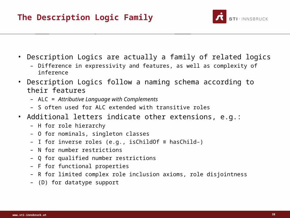
The Description Logic Family
• Description Logics are actually a family of related logics– Difference in expressivity and features, as well as complexity of inference
• Description Logics follow a naming schema according to their features
– ALC = Attributive Language with Complements– S often used for ALC extended with transitive roles
• Additional letters indicate other extensions, e.g.:– H for role hierarchy– O for nominals, singleton classes– I for inverse roles (e.g., isChildOf ≡ hasChild–)– N for number restrictions– Q for qualified number restrictions– F for functional properties– R for limited complex role inclusion axioms, role disjointness– (D) for datatype support
38
www.sti-innsbruck.at
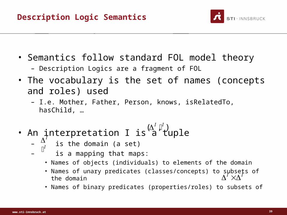
Description Logic Semantics
• Semantics follow standard FOL model theory– Description Logics are a fragment of FOL
• The vocabulary is the set of names (concepts and roles) used– I.e. Mother, Father, Person, knows, isRelatedTo, hasChild, …
• An interpretation I is a tuple – is the domain (a set)
– is a mapping that maps:• Names of objects (individuals) to elements of the domain• Names of unary predicates (classes/concepts) to subsets of the domain• Names of binary predicates (properties/roles) to subsets of
39
( , )I I II
I I

www.sti-innsbruck.at
Description Logic Semantics - ALC
• As an example consider the semantics of ALC– We first need to take a look at the interpretation of the basic syntax
• Interpretation I =
40
( , )I I
www.sti-innsbruck.at
Description Logic Semantics
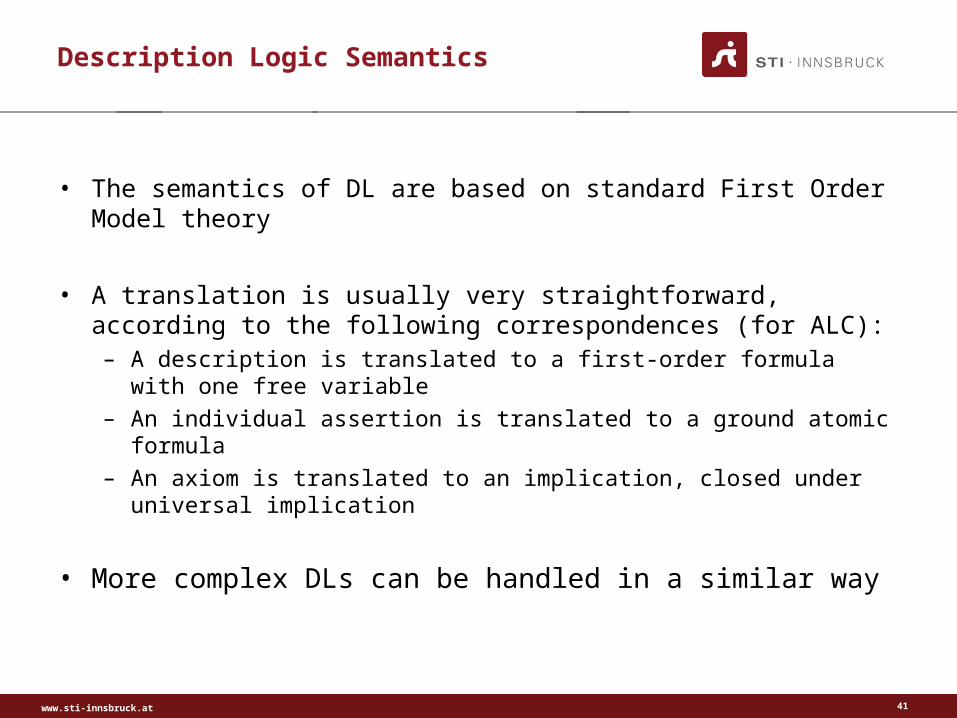
• The semantics of DL are based on standard First Order Model theory
• A translation is usually very straightforward, according to the following correspondences (for ALC):– A description is translated to a first-order formula with one free variable
– An individual assertion is translated to a ground atomic formula
– An axiom is translated to an implication, closed under universal implication
• More complex DLs can be handled in a similar way
41
www.sti-innsbruck.at
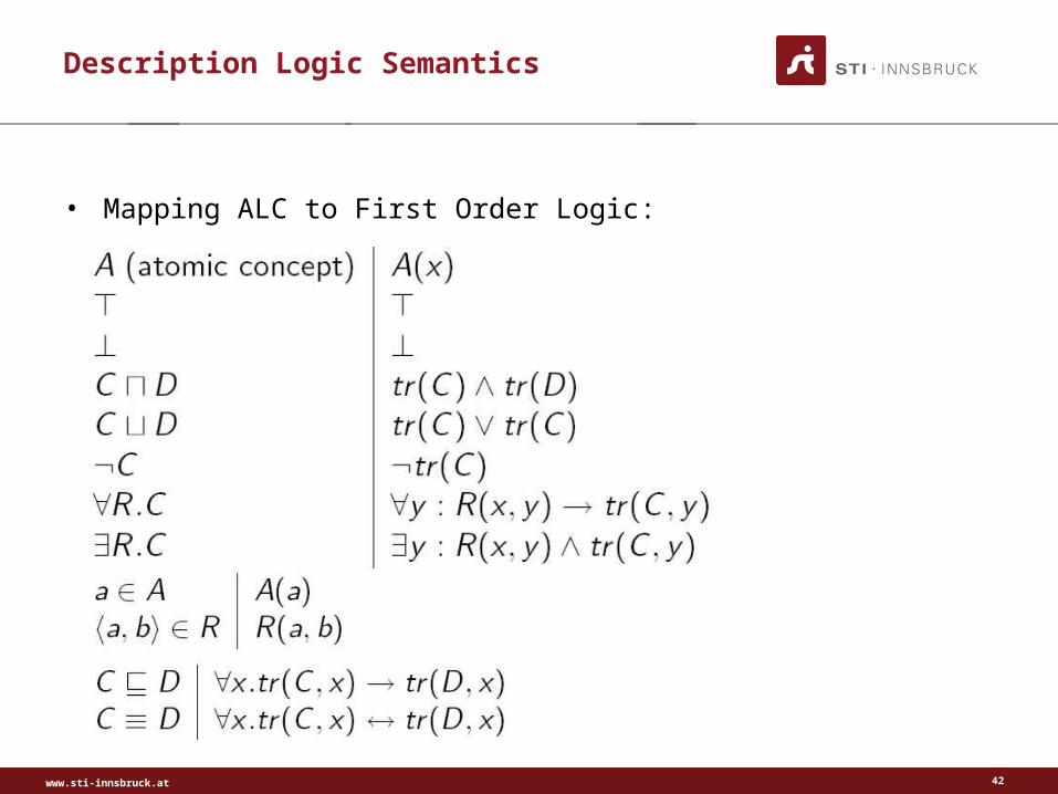
Description Logic Semantics
• Mapping ALC to First Order Logic:
42

www.sti-innsbruck.at
Description Logic Reasoning
• Main reasoning tasks for DL systems:– Satisfiability: Check if the assertions in a KB have a model– Instance checking: C(a) ? Check if an instance belongs to a
certain concept– Concept satisfiability: C ?– Subsumption: B ⊑ A ? Check if A subsumes B (if every
individual of a concept B is also of concept A)– Equivalence: A ≡ B?
• A ≡ B ⇔ B ⊑ A and A ⊑ B
– Retrieval: Retrieve a set of instances that belong to a certain concept
43
www.sti-innsbruck.at
Description Logic Reasoning
• Reasoning Task are typically reduced to KB satisfiability sat(A) w.r.t. to a knowledge base A– Instance checking: instance(a,C, A) ⇔¬sat(A ⋃ {a: ¬ C})
– Concept satisfiability: csat(C) ⇔ sat(A ⋃ {a: ¬ C})– Concept subsumption: B ⊑ A ⇔ A ⋃ {¬B ⊓ C} is not satisfiable
⇔ ¬sat(A ⋃ {¬B ⊓ C})
– Retrieval: Instance checking for each instance in the Abox
• Note: Reduction of reasoning tasks to one another in polynomial time only in propositionally closed logics
• DL reasoners typically employ tableaux algorithms to check satisfiability of a knowledge base
44
www.sti-innsbruck.at
Logic Programming
• What is Logic Programming?• Various different perspectives and definitions possible:
– Computations as deduction• Use formal logic to express data and programs
– Theorem Proving• Logic programs evaluated by a theorem prover• Derivation of answer from a set of initial axioms
– High level (non-precedural) programming language• Logic programs do not specifcy control flow• Instead of specifying how something should be computed, one states what
should be computed
– Procedural interpretation of a declarative specification of a problem• A LP systems procedurally interprets (in some way) a general declarative
statement which only defines truth conditions that should hold
45
www.sti-innsbruck.at
LOGIC PROGRAMMING
46
www.sti-innsbruck.at
Logic Programming Basics
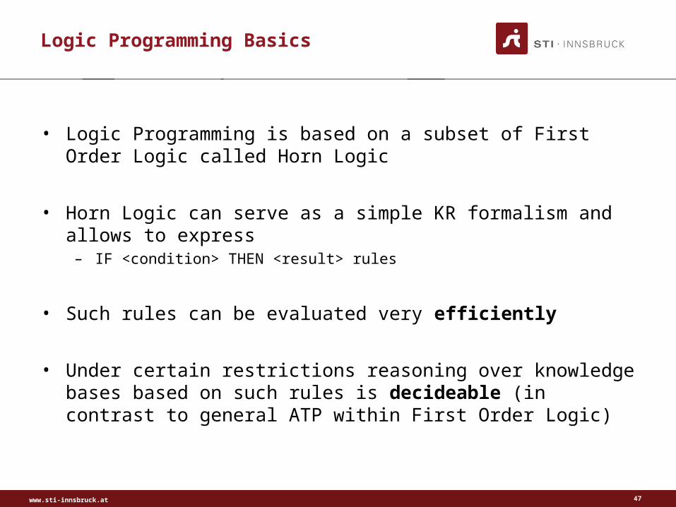
• Logic Programming is based on a subset of First Order Logic called Horn Logic
• Horn Logic can serve as a simple KR formalism and allows to express
– IF <condition> THEN <result> rules
• Such rules can be evaluated very efficiently
• Under certain restrictions reasoning over knowledge bases based on such rules is decideable (in contrast to general ATP within First Order Logic)
47
www.sti-innsbruck.at
Logic Programming Basics – Horn Logic
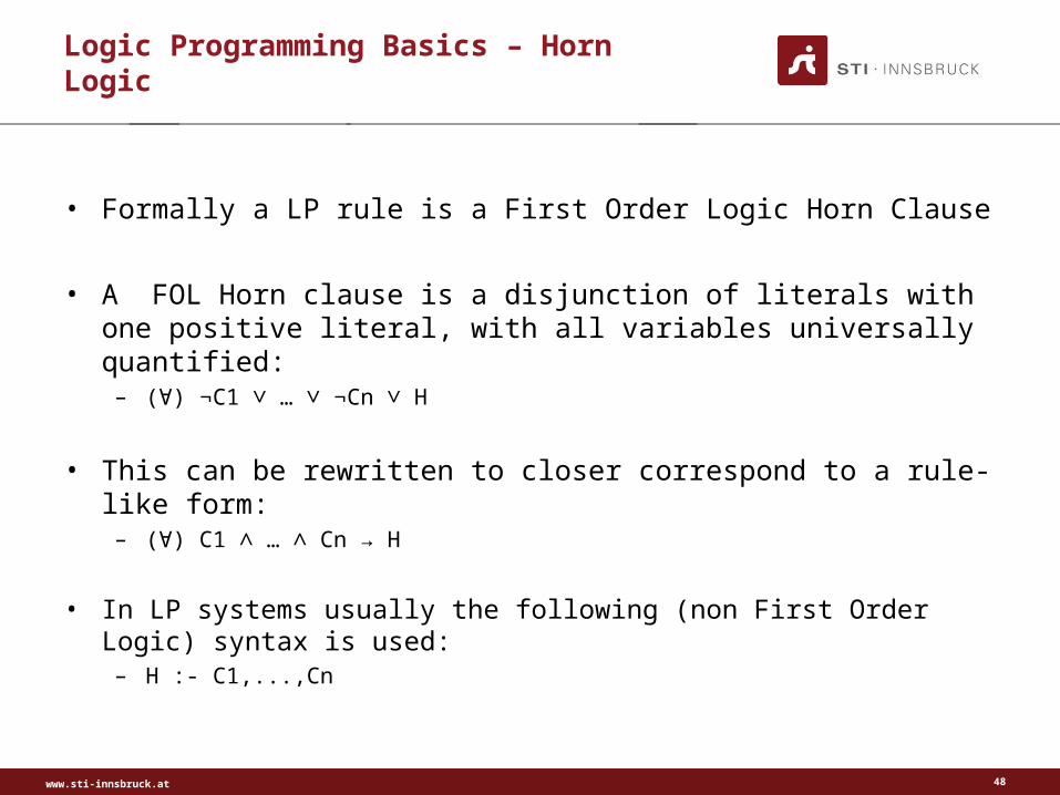
• Formally a LP rule is a First Order Logic Horn Clause
• A FOL Horn clause is a disjunction of literals with one positive literal, with all variables universally quantified:
– (∀) ¬C1 ∨ … ∨ ¬Cn ∨ H
• This can be rewritten to closer correspond to a rule-like form:– (∀) C1 ∧ … ∧ Cn → H
• In LP systems usually the following (non First Order Logic) syntax is used:
– H :- C1,...,Cn
48
www.sti-innsbruck.at
Logic Programming Syntax
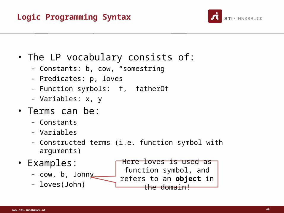
• The LP vocabulary consists of:– Constants: b, cow, “somestring”
– Predicates: p, loves
– Function symbols: f, fatherOf
– Variables: x, y
• Terms can be:– Constants
– Variables
– Constructed terms (i.e. function symbol with arguments)
• Examples:– cow, b, Jonny,
– loves(John)
49
Here loves is used as function symbol, and refers to an object
in the domain!
www.sti-innsbruck.at
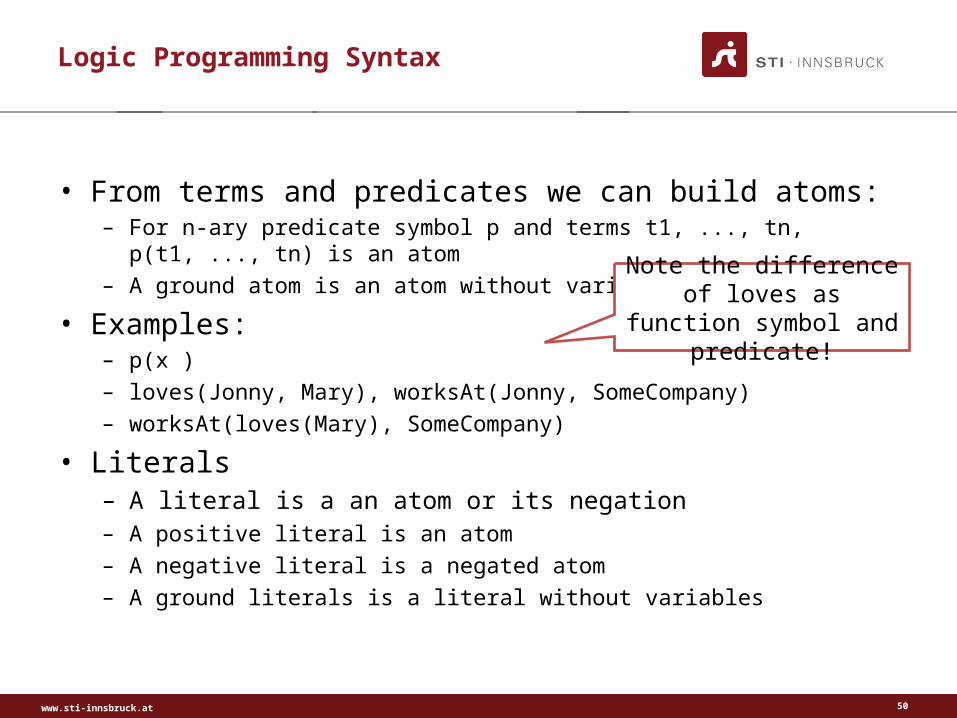
Logic Programming Syntax
• From terms and predicates we can build atoms:– For n-ary predicate symbol p and terms t1, ..., tn, p(t1, ..., tn) is an atom
– A ground atom is an atom without variables
• Examples: – p(x )
– loves(Jonny, Mary), worksAt(Jonny, SomeCompany)
– worksAt(loves(Mary), SomeCompany)
• Literals– A literal is a an atom or its negation– A positive literal is an atom
– A negative literal is a negated atom
– A ground literals is a literal without variables
50
Note the difference of loves as function symbol and
predicate!
www.sti-innsbruck.at
Logic Programming Syntax
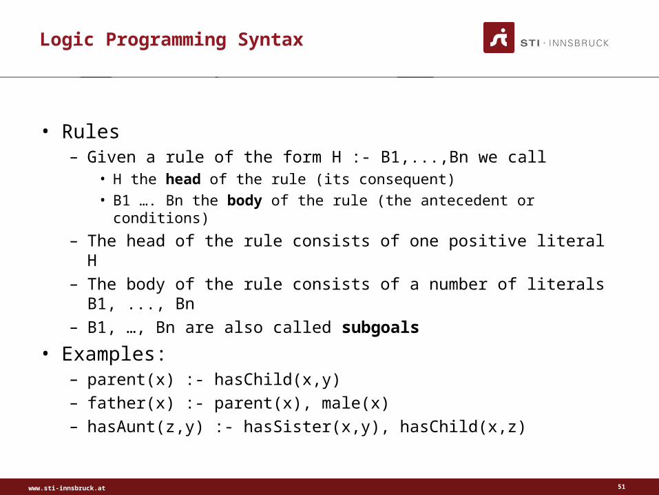
• Rules– Given a rule of the form H :- B1,...,Bn we call
• H the head of the rule (its consequent)
• B1 …. Bn the body of the rule (the antecedent or conditions)
– The head of the rule consists of one positive literal H– The body of the rule consists of a number of literals B1, ..., Bn– B1, …, Bn are also called subgoals
• Examples:– parent(x) :- hasChild(x,y)– father(x) :- parent(x), male(x)– hasAunt(z,y) :- hasSister(x,y), hasChild(x,z)
51

www.sti-innsbruck.at
Logic Programming Syntax
• Facts denote assertions about the world:– A rule without a body (no conditions)– A ground atom
• Examples:– hasChild(Jonny, Sue)– Male(Jonny)).
• Queries allow to ask questions about the knowledge base:– Denoted as a rule without a head:
• ?- B1,...,Bn.
• Examples:– ? - hasSister(Jonny,y), hasChild(Jonny , z) gives all the sisters and children of
Jonny– ? - hasAunt(Mary,y) gives all the aunts of Mary– ?- father(Jonny) ansers if Jonny is a father
52
www.sti-innsbruck.at
Logic Programming - Recursion
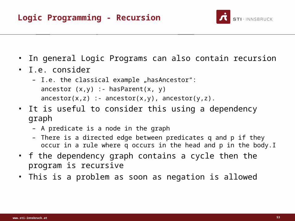
• In general Logic Programs can also contain recursion• I.e. consider
– I.e. the classical example „hasAncestor“:
ancestor (x,y) :- hasParent(x, y)
ancestor(x,z) :- ancestor(x,y), ancestor(y,z).
• It is useful to consider this using a dependency graph– A predicate is a node in the graph– There is a directed edge between predicates q and p if they occur in a rule where
q occurs in the head and p in the body.I
• f the dependency graph contains a cycle then the program is recursive
• This is a problem as soon as negation is allowed
53

www.sti-innsbruck.at
Logic Programming - Subsets
• Full Logic Programming– Allows function symbols– Does not allow negation– Is turing complete
• Full Logic Programming is not decideable– Prolog programs are not guaranteed to terminate
• Several ways to guarantee the evaluation of a Logic Program– One is to enforce syntactical restrictions– This results in subsets of full logic programming– Datalog is such a subset
54

www.sti-innsbruck.at
Logic Programing - Datalog
• Datalog is a syntactic subset of Prolog– Originally a rule and query language for deductive databases
• Considers knowledge bases to have two parts– Extensional Database (EDB) consists of facts– Intentional Database(IDB) consists of non-ground rules
• Restrictions:1. Datalog disallows function symbols
2. Imposes stratification restrictions on the use of recursion + negation
3. Allows only range restricted variables (safe variables)
• Safe Variables:– Only allows range restricted variables, i.e. each variable in the conclusion of a
rule must also appear in a not negated clause in the premise of this rule.– This limits evaluation of variables to finitely many possible bindings
55
www.sti-innsbruck.at
Logic Programming - Datalog
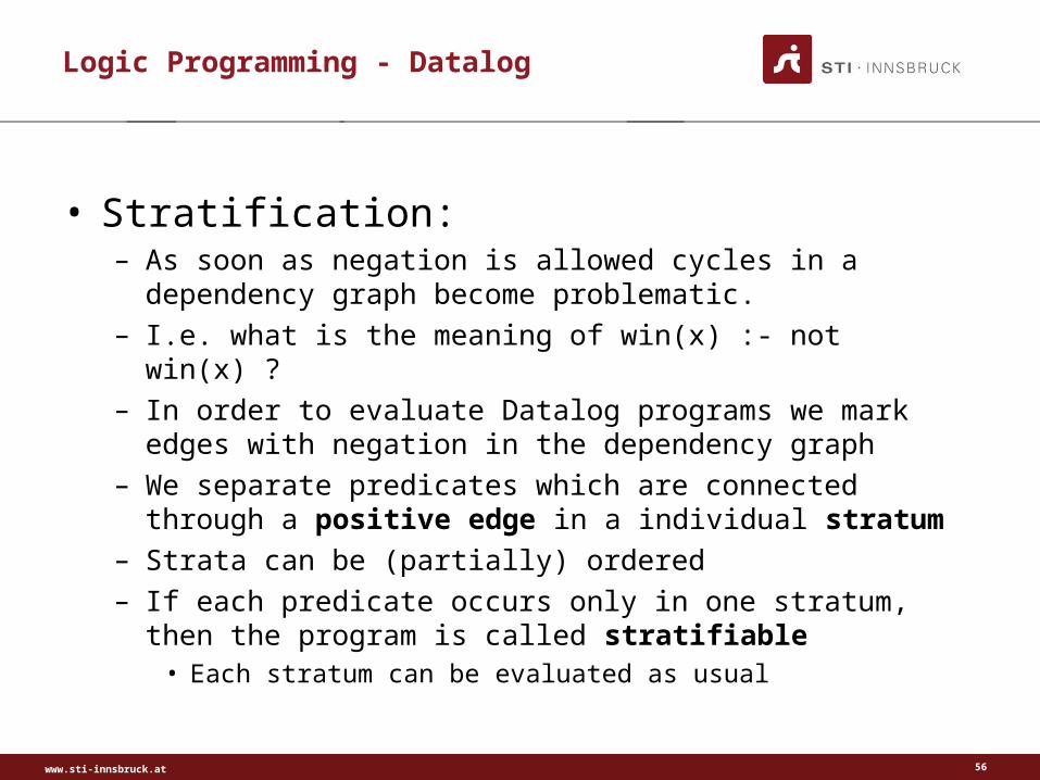
• Stratification:– As soon as negation is allowed cycles in a dependency graph
become problematic.– I.e. what is the meaning of win(x) :- not win(x) ?– In order to evaluate Datalog programs we mark edges with
negation in the dependency graph– We separate predicates which are connected through a positive
edge in a individual stratum– Strata can be (partially) ordered– If each predicate occurs only in one stratum, then the program is
called stratifiable• Each stratum can be evaluated as usual
56

www.sti-innsbruck.at
Logic Programming - Reasoning Tasks
• The typical reasoning task for LP systems is query answering– Ground queries, i.e. ?- loves(Mary, Joe)
– Non-ground query, i.e. ?- loves(Mary, x)
• Non-ground queries can be reduced to a series of ground queries– ?- loves(Mary, x)
– Replace x by every possible value
• In Logic Programming ground queries are equivalent to entailment of facts– Answering ?- loves(Mary, Joe) w.r.t. a knowledge base A is equivalent
to checking
A ⊧ loves(Mary, Joe)
57
www.sti-innsbruck.at
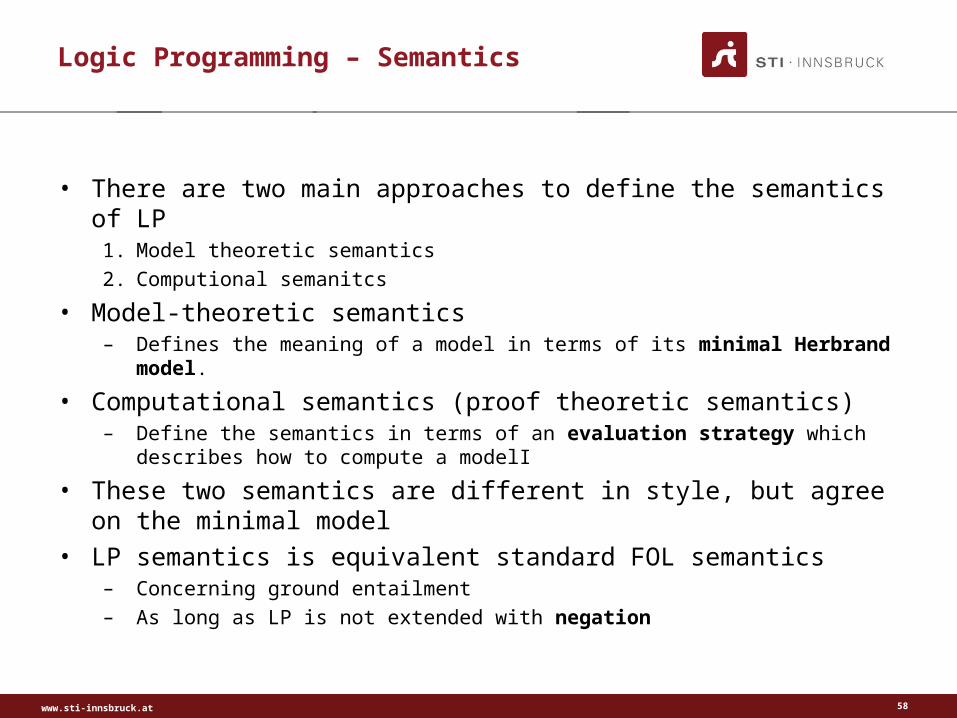
Logic Programming – Semantics
• There are two main approaches to define the semantics of LP1. Model theoretic semantics
2. Computional semanitcs
• Model-theoretic semantics– Defines the meaning of a model in terms of its minimal Herbrand model.
• Computational semantics (proof theoretic semantics)– Define the semantics in terms of an evaluation strategy which describes how to
compute a modelI
• These two semantics are different in style, but agree on the minimal model
• LP semantics is equivalent standard FOL semantics– Concerning ground entailment– As long as LP is not extended with negation
58
www.sti-innsbruck.at
Logic Programming – Semantics
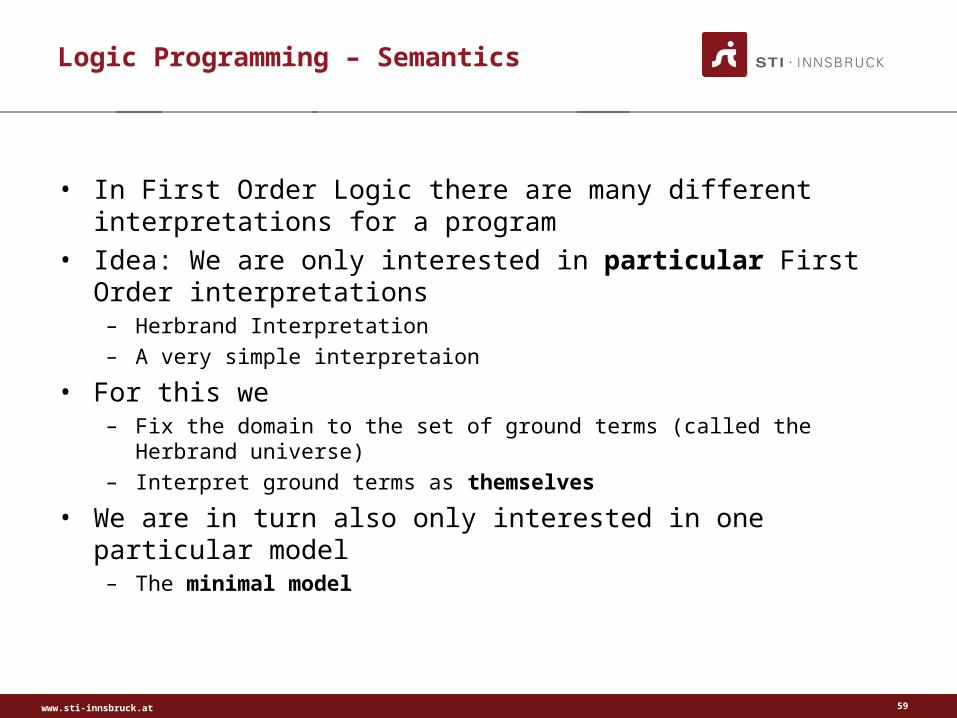
• In First Order Logic there are many different interpretations for a program
• Idea: We are only interested in particular First Order interpretations– Herbrand Interpretation– A very simple interpretaion
• For this we– Fix the domain to the set of ground terms (called the Herbrand universe)– Interpret ground terms as themselves
• We are in turn also only interested in one particular model – The minimal model
59
www.sti-innsbruck.at
Logic Programming – Semantics
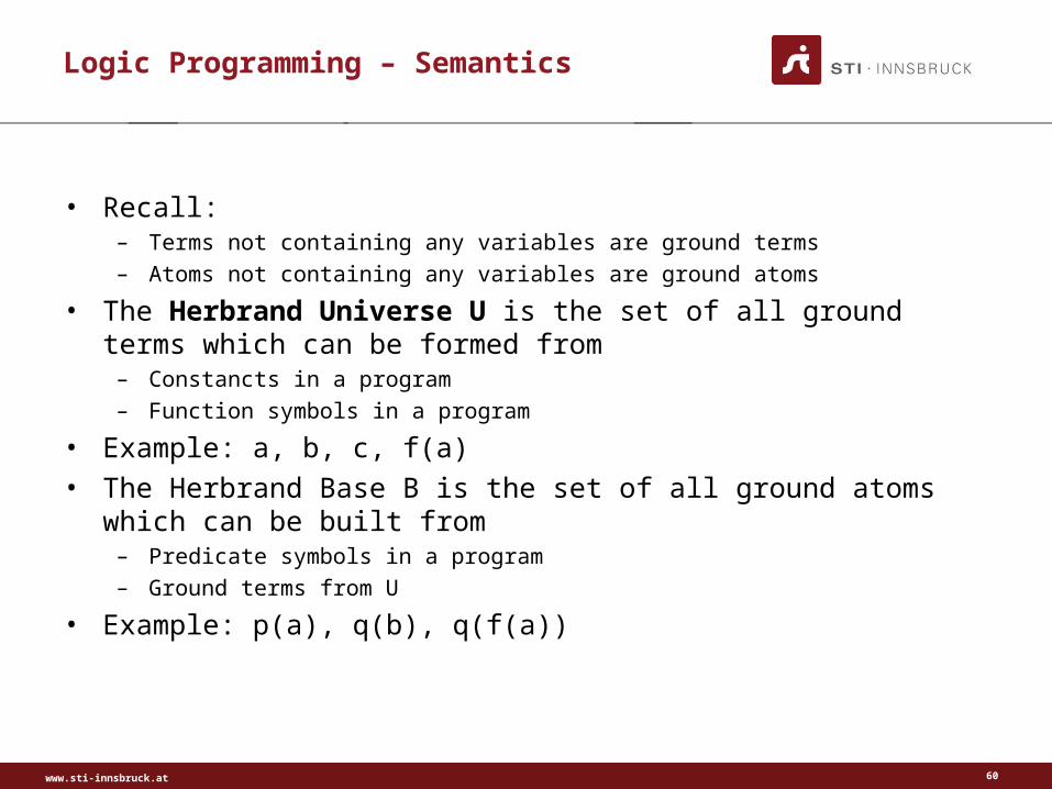
• Recall:– Terms not containing any variables are ground terms– Atoms not containing any variables are ground atoms
• The Herbrand Universe U is the set of all ground terms which can be formed from
– Constancts in a program– Function symbols in a program
• Example: a, b, c, f(a)• The Herbrand Base B is the set of all ground atoms which can be built
from– Predicate symbols in a program– Ground terms from U
• Example: p(a), q(b), q(f(a))
60

www.sti-innsbruck.at
Logic Programming – Semantics
• A Herbrand Interpretation I is a subset of the Herbrand Base B for a program
• A Herbrand Model M is a Herbrand Interpretation which makes every formula true, so:– Every fact from the program is in M
– For every rule in the program: If every positive literal in the body is in M, then the literal in the head is also in M
• The model of a Logic Program P is the least Herbrand Model– This least Herbrand Model is the inersection of all Herbrand Models
– This model is uniquely defined for every Program
→ A very intuitive and easy way to capture the sematnics of LP
61

www.sti-innsbruck.at
Logic Programming - Negation
• How do we handle negation in Logic Programs?• Horn Logic only permits negation in limited form
– Consider (∀) ¬C1 ∨ … ∨ ¬Cn ∨ H
• Special solution: Negation-as-failure (NAF): – Whenever a fact is not entailed by the knowledge base, its negation is entailed– This is a form of “Default reasoning”– This introduces non-monotonic behavior (previous conclusions might need to be
revised during the inference process)
• NAF is not classical negation and pushes LP beyond classical First Order Logic
• This allows a form of negation in rules:– (∀) C1 ∧ … ∧ Ci ∧ not Cn → H– H :- B1, … Bi, not Bn
62

www.sti-innsbruck.at
SUMMARY
63

www.sti-innsbruck.at
Summary
• Basic syntactic building blocks– Concepts– Roles– Individuals
• Limited constructs for building complex concepts, roles• Many different Description Logics exist, depending on choice of
constructs• Set-based term descriptions• Implicit knowledge can be inferred automatically
– Main reasoning task: Subsumption– Usually reasoning tasks in DLs can all be reduced to satisfiablity checking
• Efficient Tbox (schema) reasoning• ABox reasoning (query answering) do not scale so well
64
www.sti-innsbruck.at
REFERENCES
65

www.sti-innsbruck.at
References and Further Information
• [1] Uwe Schöning, Logic for Computer Scientists (2nd edition), 2008, Birkhäuser (Chapter 2 & 3)
• [2] Alan Robinson and Andrei Voronkov, Handbook of Automated Reasoning, Volume I (Chapter 2)
• [3] Michael Huth and Mark Ryan, Logic in Computer Science(2nd edition) , 2004, Cambridge University Press
• [4] M. Fitting: First-Order Logic and Automated Theorem Proving, 1996 Springer-Verlag New York (Chapter 5)
66
www.sti-innsbruck.at 67
# Date Title
1 Introduction
2 Propositional Logic
3 Predicate Logic
4 Theorem Proving, Logic Programming, and Description Logics
5 Search Methods
6 CommonKADS
7 Problem Solving Methods
8 Planning
9 Agents
10 Rule Learning
11 Inductive Logic Programming
12 Formal Concept Analysis
13 Neuronal Networks
14 Semantic Web and Exam Preparation
Next Lecture
www.sti-innsbruck.at 68
Questions?