Written Assignment 2:Investigating Curvature

CMU 15-458/858B (Spring 2019)

Submission Instructions. Please submit your solutions to the exercises (whether handwritten, LaTeX, etc.)as a single PDF file by email to Geometry.Collective@gmail.com. This email must also contain the .zip filefor your coding solution. Scanned images/photographs can be converted to a PDF using applications likePreview (on Mac) or a variety of free websites (e.g., http://imagetopdf.com). Your submission email mustinclude the string DDG19A2 in the subject line. Your graded submission will (hopefully!) be returned toyou at least one day before the due date of the next written assignment.

Grading. Please clearly show your work. Partial credit will be awarded for ideas toward the solution,so please submit your thoughts on an exercise even if you cannot find a full solution. Note that you arerequired to complete only TWO exercises from each of sections 1, 2, 3, and 4! (8 problems total.) You areof course welcome to do more. :-)

If you don’t know where to get started with some of these exercises, just ask! A great way to do this is to leavecomments on the course webpage under this assignment; this way everyone can benefit from your questions.We are glad to provide further hints, suggestions, and guidance either here on the website, via email, or inperson. Office hours are listed on the course website, but let us know if you’d like to arrange an individualmeeting.

Late Days. Note that you have 5 no-penalty late days for the entire course, where a “day” runs from6:00:00 PM Eastern to 5:59:59 PM Eastern the next day. No late submissions are allowed once all late days areexhausted. If you wish to claim one or more of your five late days on an assignment, please indicate whichlate day(s) you are using in your email submission. You must also draw Platonic solids corresponding tothe late day(s) you are using (cube=1, tetrahedron=2, octahedron=3, dodecahedron=4, icosahedron=5). Usethem wisely, as you cannot use the same polyhedron twice! If you are typesetting your homework on thecomputer, we have provided images that can be included for this purpose (in LATEX these can be includedwith the \includegraphics command in the graphicx package).

Collaboration and External Resources. You are strongly encouraged to discuss all course material withyour peers, including the written and coding assignments. You are especially encouraged to seek out newfriends from other disciplines (CS, Math, Engineering, etc.) whose experience might complement your own.However, your final work must be your own, i.e., direct collaboration on assignments is prohibited.

You are allowed to refer to any external resources except for homework solutions from previous editionsof this course (at CMU and other institutions). If you use an external resource, cite such help on yoursubmission. If you are caught cheating, you will get a zero for the entire course.

Warning! With probability 1, there are typos in this assignment. If anything in this handout does notmake sense (or is blatantly wrong), let us know! We will be handing out extra credit for good catches. :-)

1

Format. This written assignment is cement your understanding of curvature on both continuous anddiscrete surfaces.

This assignment is closely connected to Chapters 3, 4, and 5 of the course notes. Additionally, the courseslides (as they are released) will be extremely helpful for completing the assignment.

1 Smooth Curves and Surfaces

Warning! You are required to do Exercise 4 of this section.

1. Consider the curve γ : R→ R3 defined by

γ(s) := (s, s2, s3).

(a) Compute dds γ and T(s).

(b) Compute κ(s) and N(s).

(c) Compute B(s) and τ(s).

2. Consider the map f : R2 → R3 defined by

f (u, v) :=1

u2 + v2 + 1(2u, 2v, u2 + v2 − 1).

(a) Verify that for all (u, v) ∈ R2, f (u, v) lies on the unit sphere centered at the origin.

(b) Explicitly compute the differential df .

(c) Compute the metric g induced by f .

(d) Compute the Gauss map N induced by f .

(e) Compute the corresponding shape operator dN.

3. Consider the immersion of the torus f : [0, 2π]× [0, 2π]→ R3 defined by

f (θ, ϕ) := ((R + r cos ϕ) cos θ, (R + r cos ϕ) sin θ, r sin ϕ)

where R > r > 0.

(a) Explicitly compute the differential df .

(b) Compute the metric g induced by f .

(c) Compute the Gauss map N induced by f .

(d) Compute the corresponding shape operator dN.

4. [Required] Recall that the mean and Gaussian curvature can be expressed in terms of the principalcurvatures κ1, κ2:

H :=κ1 + κ2

2, K := κ1κ2.

Derive expressions for κ1 and κ2 in terms of H and K. (For this exercise you do not need to worry aboutwhether κ1 > κ2 or κ2 > κ1.)

2

2 Discrete Curvature, Part I: Surface Normals

Warning! In several of the exercises in this section you are asked to derive an expression for the gradient ofsome geometric quantity. For these questions we ask that you use geometric arguments rather than simplytaking the partial derivatives. (Solutions that compute the gradient via partial derivatives will not receiveany credit.) The basic recipe for obtaining the gradient geometrically is:

• First, find the unit vector such that moving in that direction increases the quantity the fastest. Thisdirection gives the direction of the gradient.

• Next, find the rate of change when moving in this direction. This quantity gives the magnitude of thegradient.

To make this idea clear, here is a concrete example:

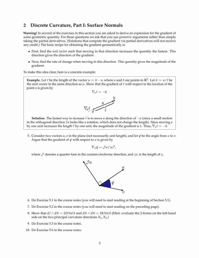
Example. Let ` be the length of the vector u := b− a, where a and b are points in R2. Let u := u/` bethe unit vector in the same direction as u. Show that the gradient of ` with respect to the location of thepoint a is given by

∇a` = −u.

Solution. The fastest way to increase ` is to move a along the direction of −u (since a small motionin the orthogonal direction Ju looks like a rotation, which does not change the length). Since moving aby one unit increases the length ` by one unit, the magnitude of the gradient is 1. Thus, ∇a` = −u.

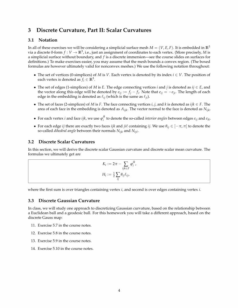
5. Consider two vectors u, v in the plane (not necessarily unit length), and let ψ be the angle from u to v.Argue that the gradient of ψ with respect to u is given by

∇uψ = J u/|u|2,

where J denotes a quarter turn in the counter-clockwise direction, and |u| is the length of u.

6. Do Exercise 5.1 in the course notes (you will need to start reading at the beginning of Section 5.1).

7. Do Exercise 5.2 in the course notes (you will need to start reading on the preceding page).

8. Show that d f ∧ dN = 2HNdA and dN ∧ dN = 2KNdA (Hint: evaluate the 2-forms on the left-handside on the two principal curvature directions X1, X2.)

9. Do Exercise 5.3 in the course notes.

10. Do Exercise 5.6 in the course notes.

3

3 Discrete Curvature, Part II: Scalar Curvatures

3.1 Notation

In all of these exercises we will be considering a simplicial surface mesh M = (V, E, F). It is embedded in R3

via a discrete 0-form f : V → R3, i.e., just an assignment of coordinates to each vertex. (More precisely, M isa simplicial surface without boundary, and f is a discrete immersion—see the course slides on surfaces fordefinitions.) To make exercises easier, you may assume that the mesh bounds a convex region. (The boxedformulas are however ultimately valid for nonconvex meshes.) We use the following notation throughout:

• The set of vertices (0-simplices) of M is V. Each vertex is denoted by its index i ∈ V. The position ofeach vertex is denoted as fi ∈ R3.

• The set of edges (1-simplices) of M is E. The edge connecting vertices i and j is denoted as ij ∈ E, andthe vector along this edge will be denoted by eij := f j − fi. Note that eij = −eji. The length of eachedge in the embedding is denoted as `ij (which is the same as `ji).

• The set of faces (2-simplices) of M is F. The face connecting vertices i, j, and k is denoted as ijk ∈ F. Thearea of each face in the embedding is denoted as Aijk. The vector normal to the face is denoted as Nijk.

• For each vertex i and face ijk, we use ϕjki to denote the so-called interior angles between edges eij and eik.

• For each edge ij there are exactly two faces ijk and ji` containing ij. We use θij ∈ [−π, π] to denote theso-called dihedral angle between their normals Nijk and Nij`.

3.2 Discrete Scalar Curvatures

In this section, we will derive the discrete scalar Gaussian curvature and discrete scalar mean curvature. Theformulas we ultimately get are

Ki := 2π − ∑ijk∈F

ϕjki ,

Hi := 12 ∑

ijθij`ij,

where the first sum is over triangles containing vertex i, and second is over edges containing vertex i.

3.3 Discrete Gaussian Curvature

In class, we will study one approach to discretizing Gaussian curvature, based on the relationship betweena Euclidean ball and a geodesic ball. For this homework you will take a different approach, based on thediscrete Gauss map:

11. Exercise 5.7 in the course notes.

12. Exercise 5.8 in the course notes.

13. Exercise 5.9 in the course notes.

14. Exercise 5.10 in the course notes.

4

3.4 Steiner Formula for Simpicial Surfaces

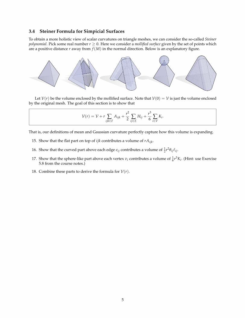
To obtain a more holistic view of scalar curvatures on triangle meshes, we can consider the so-called Steinerpolynomial. Pick some real number r ≥ 0. Here we consider a mollified surface given by the set of points whichare a positive distance r away from f (M) in the normal direction. Below is an explanatory figure.

Let V(r) be the volume enclosed by the mollified surface. Note that V(0) = V is just the volume enclosedby the original mesh. The goal of this section is to show that

V(r) = V + r ∑ijk∈F

Aijk +r2

2 ∑ij∈E

Hij +r3

6 ∑i∈V

Ki.

That is, our definitions of mean and Gaussian curvature perfectly capture how this volume is expanding.

15. Show that the flat part on top of ijk contributes a volume of rAijk.

16. Show that the curved part above each edge eij contributes a volume of 12 r2θij`ij.

17. Show that the sphere-like part above each vertex vi contributes a volume of 16 r3Ki. (Hint: use Exercise

5.8 from the course notes.)

18. Combine these parts to derive the formula for V(r).

5

4 Discrete Curvature, Part III: Curvature Normals

In the previous section, we derived the discretizations of mean and Gaussian curvature. In this section, wederive discretizations of their normal counterparts: HN and KN.

In the following exercises, the following theorems will be useful.Discrete Gauss-Bonnet Theorem.

∑i∈V

(2π − ∑

ijk∈Fϕ

jki

)= 2πχ(M),

where χ(M) is the Euler Characteristic of the surface.Schlafli formula. For every i ∈ V

∑jk∈E

(∇ fiθjk)`jk = 0.

In Chapter 5 of the course notes, it is shown that taking the gradient of total volume V with respect to theposition fi of vertex i yields a discretization for area normal NdA—specifically, we get the area-weighted sumof the face normals:

∇ fiV =

13 ∑

ijk∈FAijk Nijk.

In the following exercises, you will show that the gradient of a sequence of quantities (total volume, totalarea, total mean curvature, total Gauss curvature) yields a corresponding sequence of discrete curvaturenormals (area normal, mean curvature normal, Gauss curvature normal, zero).

19. Show that when we take the gradient of the total surface area with respect to the position of one of thevertices, we instead get

∇ fi ∑ijk∈F

Aijk =12 ∑

ij∈E(cot αij + cot βij)( f j − fi),

where αij and βij are the two interior angles opposite edge ij. The right-hand-side is a discretization ofthe mean curvature normal HN at vertex vi.

20. Next, show that the gradient of the total discrete scalar mean curvature gives

∇ fi

12 ∑

jk∈Eθjk`jk =

12 ∑

ij∈E

θij

`ij( f j − fi).

The right-hand-side is a discretization of the Gauss curvature normal KN at vertex vi.

21. Finally, show that the gradient of the total discrete scalar Gauss curvature is zero:

∇ fi ∑`∈V

[2π − ∑

jk`∈Fϕ

jk`

]= 0.

(Hint: there is a way to do this with almost no calculation.)

6