Write-ecient Algorithms

Yan Gu

CMU-CS-18-113

September, 2018

School of Computer ScienceCarnegie Mellon University

Pittsburgh, PA 15213

Thesis Committee:

Guy E. Blelloch, ChairPhillip B. Gibbons

Anupam GuptaJeremy T. Fineman (Georgetown University)

Julian Shun (MIT)

Submitted in partial fulllment of the requirementsfor the degree of Doctor of Philosophy.

Copyright © 2018 Yan Gu

This research was sponsored by Intel and the National Science Foundation under grant numbers CCF-1018188, CCF-1314590, and CCF-1533858. The views and conclusions contained in this document are thoseof the author and should not be interpreted as representing the ocial policies, either expressed or implied,of any sponsoring institution, the U.S. government or any other entity.

Keywords: Write-Ecient Algorithms, Non-Volatile Memory, Asymmetric Read andWrite Cost, Computational Model, Parallel Algorithms

To my family.

Abstract

New non-volatile memory (NVM) technologies are projected to becomethe dominant type of main memory in the near future. They promise byte-addressability, good read latencies, and signicantly lower energy and higherdensity compared to DRAM. However, a key property of NVMs is the asym-metric read and write cost: write operations are much more expensive thanreads regarding energy, bandwidth, and latency. This property contradictsfty years of classic algorithms research that has focused on the setting inwhich reads and writes have similar cost, and poses the need to developwrite-ecient algorithms that use fewer writes than the classic approaches.

This thesis provides a comprehensive study of the design and analysisof write-ecient algorithms, which includes computational models, lowerbounds, algorithms, and experimental validations. More specically, thisthesis rst presents and studies several models that account for read-writeasymmetry in dierent settings (sequential, parallel, I/O models, etc.). Then,a number of lower bounds are shown, which indicate the hardness of asymp-totically improving some classic algorithms under certain assumptions.

The main contribution of this thesis consists of new write-ecient al-gorithms for fundamental algorithms in Computer Science, from basic al-gorithmic building blocks (sorting, reduce, lter, etc.), to graph algorithms((bi)connectivity, shortest paths, MST, BFS, etc.), geometric algorithms anddata structures (convex hull, Delaunay triangulation, k-d trees, augmentedtrees, etc.), as well as many cache-oblivious algorithms for dynamic program-ming and linear algebra problems. The numbers of writes in all algorithmsstudied in this thesis are signicantly reduced asymptotically. Furthermore,most of these algorithms are also highly parallel. Many techniques used toobtain these results are of independent interest, since they are applicable tomany other problems outside those studied in this thesis, and lead to improvedalgorithms in the classic setting without read-write asymmetry.

This thesis also proposes the rst experimental framework to analyzethe performance of write-ecient algorithms in practice, and conducts ex-periments on a variety of algorithms. The experimental results show theeectiveness of write-ecient algorithms, and suggest that the algorithmsdeveloped in this thesis may be of both theoretical and practical interest.

Acknowledgement

It is surprising that I had not known my advisor Guy Blelloch before accepting the oer tobecome a graduate student at CMU. However, when I rst met him during his IC class wherehe was talking about his parallel MIS algorithm, I discovered the kind of research I had soughtfor years. I consider myself lucky to be Guy’s student without a related research background,despite the false perception of his unpopularity and lack of attraction for other students.

Jokes apart, I owe my deepest gratitude to Guy, the best advisor that one could imagine. Hehas always been a great mentor and an extremely patient teacher. I especially thank him forletting me have the freedom of exploring my true research interests over the course of these sixyears, and supporting me no matter what I was working on, from computer graphics in the rstyears, several random topics in the middle, and eventually this thesis. I could not have asked fora better advisor.

I would also like to thank the rest of my thesis committee members. Other than helping methroughout my 6-year graduate studies and providing me with useful feedback to improve thisthesis, they have all inuenced me signicantly with regard to both research and career paths.

Phil Gibbons is an encyclopedia of computer science. He can always propose insightfulthoughts and long-term pictures of research work, and novel ideas for research challenges. Heprovided me thorough explanations of my trivial and non-trivial questions. I have learned a lotfrom Phil during our weekly meetings, and without him I would not have this thesis.

I have taken, audited and helped with (as a TA) many of Anupam Gupta’s courses. I wasimpressed by his expertise in mathematics and thorough understanding of algorithms, andthereby realizing how attractive and sexy an algorithm researcher can be. He is one of the keyfactors for my switch to algorithm design as my research topic.

Jeremy Fineman is an encyclopedia of algorithms. In our discussions, he seems to understandthe details of all the algorithms that were proposed in the last decade or back in the 1980s. Hiserudite knowledge in algorithms and quick reaction helped in developing many of the results inthis thesis. From Jeremy and my other committee members, I comprehended that I needed toput in a lifelong eort to become a great researcher like them in the future.

Unlike other committee members, Julian Shun had partial overlap with me as a graduatestudent at CMU. I am fortunate to have collaborated with Julian on about half of my papersat CMU, and I have learned so many useful skills from him, such as conducting research,background study, paper writing, and even the spirit of diligence. The only pity I nurse is that Icould have collaborated with and learned from him earlier, instead of my third year as he wasgraduating.

Research is a team eort, and I was fortunate to have my collaborators and our researchgroup. I would like to thank my other co-authors, Naama Ben-David, Kayvon Fatahalian, YongHe, Charles McGuey, Yihan Sun, and Kanat Tangwongsan for contributing their ideas andeort in all the papers I have worked on at CMU. I am thankful to Umut Acar, Laxman Dhulipala,Yuanhao Wei, Sam Westrick, Shen Chen Xu and Yu Zhao for the valuable discussions and

feedback of my research work and talks, and I am looking forward to the chance to collaboratewith all of them. I specially thank Charles and Laxman for their help on the writing of thisthesis. I also thank all those who were previously mentioned and my other PhD friends at CMU.Although we work on dierent areas, our frequent chats help me in guring the entire computerscience world more (and gossip), which is very benecial for me.

During my graduate studies, I was lucky to have had the opportunity to interact with manyother faculty members at CMU. I would like to give my special thanks to Kayvon Fatahalian andDanny Sleator, who granted me lots of assistance with regard to both school work and dailyissues during the rst several years when I was still a helpless foreigner. I had the opportunityto work as a teaching assistant for Anupam, Danny, Guy, and Kayvon, and from them I learnedhow to become more eective at teaching. I also thank Kayvon, Danny, Phil, and Bob Harper forhelping me with my speaking and writing skills requirements, and Kayvon and Guy for trustingme to give several lectures in their classes.

I spent my rst two years at CMU as a member of the Graphics lab. I thank the facultymembers Kayvon, Alexei Efros, Jessica Hodgins, Nancy Pollard, Yaser Sheikh, Adrien Treuille,and the students for their help on my research and presentation skills. I would like to give myspecial thanks to Nancy. She was the rst professor I met at CMU as an undergrad. She alsokindly provided me a considerable amount of assistance on my application, helped me settledown in Pittsburgh, and conducted mock interview for my practice. I have nothing to oer inreturn other than my gratitude.

My journey at CMU would be a dull one without my friends. Our team Stuck in Mitosisparticipated in many intramural sports for years, and I also enjoyed the table tennis club in ourdepartment. As a Chinese, the Chinese cuisine parties were always a kind of expectancy formy busy PhD life. I thank Yu for his once-a-semester hotpot parties and many other hosts inPittsburgh, and my friends regularly coming to my house to enjoy our cooking, including FanYang, Fei Fang, Haoxian Chen, Linxi Zou, Junxing Wang, Kairui Zhang, Nan Lin, Wenting Shao,Shen-Chen Xu, Yan Wang, Yanzhe Yang, Yining Wang, Yixin Luo, Yong He, Yu Zhao, ZhanpengFang, and Zhou Su. Our annual travel group comprising Yihan’s high school classmates FanGao, Lu Zheng, Tao Yu, Wanjian Tang, and Yanzhe Yin explored many places of interests in theUS, which is an excellent memory of my PhD journey.

I would like to express my earnest gratitude to my parents. Naming me Yan which meansresearch, they cultivated my interests in science and exploring this world. It would have beenimpossible for me to be at the position without their inexorable love, support, and encouragement.

Finally, I am indebted to the support of my beloved wife Yihan Sun. Her unconditional andconstant love, patience, support and encouragement made my PhD career extremely enjoyable.Yihan is also a wonderful co-author, a 24/7 collaborator with whom I can discuss my researchideas and progress, a great audience who consistently provided valuable feedbacks, and a mentorwho forces me to think about long-term scenarios regarding both research and life. I cannotimagine how my life would be like without her.

Contents

1 Introduction 1

1.1 Motivations for Write-Ecient Algorithms . . . . . . . . . . . . . . . . . 41.1.1 Read-Write Asymmetry in Emerging Non-Volatile Memories . . . 51.1.2 Persistency and Other System-Level Considerations . . . . . . . 61.1.3 Intellectual Curiosity . . . . . . . . . . . . . . . . . . . . . . . . . 7

1.2 Computational Models . . . . . . . . . . . . . . . . . . . . . . . . . . . . 81.3 Overview of Lower Bounds . . . . . . . . . . . . . . . . . . . . . . . . . . 111.4 Overview of Write-Ecient Algorithms . . . . . . . . . . . . . . . . . . . 12

1.4.1 Basic Algorithmic Building Blocks . . . . . . . . . . . . . . . . . 121.4.2 Graph Algorithms . . . . . . . . . . . . . . . . . . . . . . . . . . 131.4.3 Geometric Algorithms . . . . . . . . . . . . . . . . . . . . . . . . 161.4.4 Cache-Oblivious Algorithms for Dynamic Programming and Lin-

ear Algebra . . . . . . . . . . . . . . . . . . . . . . . . . . . . . . 181.5 Experimental Validation . . . . . . . . . . . . . . . . . . . . . . . . . . . 191.6 Organization of this Thesis . . . . . . . . . . . . . . . . . . . . . . . . . . 211.7 Related Work . . . . . . . . . . . . . . . . . . . . . . . . . . . . . . . . . . 22

2 Models of Computation 23

2.1 Existing Sequential Computational Models . . . . . . . . . . . . . . . . . 232.1.1 Random-Access Machine Model and Time Complexity . . . . . . 232.1.2 External-Memory (EM) Model and I/O Complexity . . . . . . . . 242.1.3 Ideal-Cache Model, Cache-Oblivious (CO) Algorithms, and Cache

Complexity . . . . . . . . . . . . . . . . . . . . . . . . . . . . . . 252.2 Existing Models for Parallel Algorithms . . . . . . . . . . . . . . . . . . . 26

2.2.1 Parallel Random-Access Machine (PRAM) Model . . . . . . . . . 262.2.2 Nested-Parallel Model . . . . . . . . . . . . . . . . . . . . . . . . 27

ix

2.2.3 Work-Depth Model . . . . . . . . . . . . . . . . . . . . . . . . . . 282.2.4 Scheduling the Computation of Nested Parallelism . . . . . . . . 28

2.3 Models Accounting for Asymmetry . . . . . . . . . . . . . . . . . . . . . 302.3.1 (M,ω)-Asymmetric RAM: the Sequential Model . . . . . . . . . . 312.3.2 Asymmetric NP Model: the Parallel Model . . . . . . . . . . . . . 322.3.3 Scheduling Asymmetric NP Computations . . . . . . . . . . . . . 322.3.4 Asymmetric Ideal-Cache Model and Cache Policy . . . . . . . . . 362.3.5 Asymmetric Low-depth Cache-Oblivious Paradigm . . . . . . . . 38

3 Lower Bounds 39

3.1 General Technique in the Proofs . . . . . . . . . . . . . . . . . . . . . . . 403.2 Fast Fourier Transform (FFT) . . . . . . . . . . . . . . . . . . . . . . . . . 413.3 Sorting Networks . . . . . . . . . . . . . . . . . . . . . . . . . . . . . . . 433.4 Diamond DAG . . . . . . . . . . . . . . . . . . . . . . . . . . . . . . . . . 443.5 Results from Jacob and Sitchinava . . . . . . . . . . . . . . . . . . . . . . 45

4 Basic Algorithmic Building Blocks 47

4.1 Primitives on (M,ω)-ARAM Model . . . . . . . . . . . . . . . . . . . . . 474.2 Parallel primitives on Asymmetric NP Model . . . . . . . . . . . . . . . . 48

4.2.1 Reduce . . . . . . . . . . . . . . . . . . . . . . . . . . . . . . . . . 484.2.2 Output-Sensitive Ordered Filter . . . . . . . . . . . . . . . . . . . 49

4.3 List and Tree Contraction on Asymmetric NP Model . . . . . . . . . . . . 504.3.1 List Contraction . . . . . . . . . . . . . . . . . . . . . . . . . . . . 504.3.2 Tree Contraction . . . . . . . . . . . . . . . . . . . . . . . . . . . 51

4.4 Sorting . . . . . . . . . . . . . . . . . . . . . . . . . . . . . . . . . . . . . 564.4.1 Sorting on (M,ω)-ARAM . . . . . . . . . . . . . . . . . . . . . . . 574.4.2 Sorting on Asymmetric NP Model . . . . . . . . . . . . . . . . . . 574.4.3 Sorting on (M,B,ω)-ARAM Model . . . . . . . . . . . . . . . . . 59

4.4.3.1 Mergesort . . . . . . . . . . . . . . . . . . . . . . . . . 594.4.3.2 Sample Sort . . . . . . . . . . . . . . . . . . . . . . . . 624.4.3.3 I/O Buer Trees . . . . . . . . . . . . . . . . . . . . . . 64

4.5 Longest Common Subsequence and Edit Distance . . . . . . . . . . . . . 704.5.1 The General Case . . . . . . . . . . . . . . . . . . . . . . . . . . . 704.5.2 Smaller String Lengths . . . . . . . . . . . . . . . . . . . . . . . . 754.5.3 Recovering the Shortest Path . . . . . . . . . . . . . . . . . . . . 77

x

5 Graph Algorithms 79

5.1 Overview . . . . . . . . . . . . . . . . . . . . . . . . . . . . . . . . . . . . 795.2 Preliminaries and Terminologies . . . . . . . . . . . . . . . . . . . . . . . 805.3 Connectivity / Biconnectivity . . . . . . . . . . . . . . . . . . . . . . . . 82

5.3.1 Introduction . . . . . . . . . . . . . . . . . . . . . . . . . . . . . . 825.3.2 Related Work . . . . . . . . . . . . . . . . . . . . . . . . . . . . . 845.3.3 Implicit Decomposition . . . . . . . . . . . . . . . . . . . . . . . 855.3.4 Graph Connectivity and Spanning Forest . . . . . . . . . . . . . . 90

5.3.4.1 Low-diameter Decomposition . . . . . . . . . . . . . . 915.3.4.2 Connectivity and Spanning Forest . . . . . . . . . . . . 925.3.4.3 Connectivity Oracle in Sublinear Writes . . . . . . . . 93

5.3.5 Graph Biconnectivity . . . . . . . . . . . . . . . . . . . . . . . . . 945.3.5.1 The Classic Algorithm . . . . . . . . . . . . . . . . . . 955.3.5.2 The BC Labeling . . . . . . . . . . . . . . . . . . . . . . 955.3.5.3 Biconnectivity Oracle in Sublinear Writes . . . . . . . 975.3.5.4 Parallelizing Biconnectivity Algorithms . . . . . . . . . 103

5.3.6 Sublinear-Write Algorithms on Unbounded-Degree Graphs . . . 1035.3.7 Conclusion . . . . . . . . . . . . . . . . . . . . . . . . . . . . . . 104

5.4 Distance-based Algorithms . . . . . . . . . . . . . . . . . . . . . . . . . . 1055.4.1 Single-Source Shortest Paths . . . . . . . . . . . . . . . . . . . . . 1055.4.2 Minimum Spanning Tree (MST) . . . . . . . . . . . . . . . . . . . 107

5.4.2.1 Borůvka’s Algorithm . . . . . . . . . . . . . . . . . . . 1075.4.2.2 KKT Algorithm and the Parallel Version . . . . . . . . 108

5.4.3 Parallel Breadth-First Search . . . . . . . . . . . . . . . . . . . . . 112

6 Geometric Algorithms 115

6.1 Overview . . . . . . . . . . . . . . . . . . . . . . . . . . . . . . . . . . . . 1156.2 Iteration Dependences for RIC Algorithms . . . . . . . . . . . . . . . . . 1186.3 General Techniques for Incremental Algorithms . . . . . . . . . . . . . . 124

6.3.1 DAG Tracing . . . . . . . . . . . . . . . . . . . . . . . . . . . . . 1246.3.2 The Prex-Doubling Approach . . . . . . . . . . . . . . . . . . . 126

6.4 Comparison Sorting . . . . . . . . . . . . . . . . . . . . . . . . . . . . . . 1266.4.1 Analysis on the Iterative Dependences . . . . . . . . . . . . . . . 1266.4.2 A Linear-Write Version . . . . . . . . . . . . . . . . . . . . . . . . 128

xi

6.5 Planar Delaunay Triangulation . . . . . . . . . . . . . . . . . . . . . . . . 1296.5.1 The Work Bound . . . . . . . . . . . . . . . . . . . . . . . . . . . 1316.5.2 Analysis on the Iterative Dependences . . . . . . . . . . . . . . . 1326.5.3 A Linear-Write Version . . . . . . . . . . . . . . . . . . . . . . . . 135

6.6 Space-Partitioning Data Structures . . . . . . . . . . . . . . . . . . . . . . 1376.6.1 k-d Tree Construction and Queries . . . . . . . . . . . . . . . . . 138

6.6.1.1 Range Query . . . . . . . . . . . . . . . . . . . . . . . . 1396.6.1.2 ANN Query . . . . . . . . . . . . . . . . . . . . . . . . 1406.6.1.3 Parallel Construction and Cost Analysis . . . . . . . . 140

6.6.2 k-d Tree Dynamic Updates . . . . . . . . . . . . . . . . . . . . . . 1416.6.2.1 Logarithmic Reconstruction [224] . . . . . . . . . . . . 1426.6.2.2 Single-Tree Version . . . . . . . . . . . . . . . . . . . . 142

6.6.3 Extension to Other Trees and Queries . . . . . . . . . . . . . . . 1426.7 Augmented Trees . . . . . . . . . . . . . . . . . . . . . . . . . . . . . . . 143

6.7.1 Preliminaries and Previous Work . . . . . . . . . . . . . . . . . . 1446.7.1.1 Interval Trees and the 1D Stabbing Queries . . . . . . . 1456.7.1.2 2D Range Trees and the 2D Range Queries . . . . . . . 1456.7.1.3 Priority Search Trees and 3-sided Range Queries . . . . 145

6.7.2 The Post-Sorted Construction . . . . . . . . . . . . . . . . . . . . 1466.7.2.1 Interval Tree . . . . . . . . . . . . . . . . . . . . . . . . 1466.7.2.2 Priority Tree . . . . . . . . . . . . . . . . . . . . . . . . 147

6.7.3 Dynamic Updates using Reconstruction-Based Rebalancing . . . 1486.7.3.1 α-Labeling . . . . . . . . . . . . . . . . . . . . . . . . . 1496.7.3.2 Rebalancing Algorithm based on α-Labeling . . . . . . 1506.7.3.3 Cost Analysis of the Rebalancing . . . . . . . . . . . . 1526.7.3.4 Handling Augmented Values . . . . . . . . . . . . . . . 1536.7.3.5 Bulk Updates . . . . . . . . . . . . . . . . . . . . . . . . 154

6.8 Linear-Work Algorithms . . . . . . . . . . . . . . . . . . . . . . . . . . . 1556.8.1 Linear Programming . . . . . . . . . . . . . . . . . . . . . . . . . 1556.8.2 Closest Pair . . . . . . . . . . . . . . . . . . . . . . . . . . . . . . 1566.8.3 Smallest Enclosing Disk . . . . . . . . . . . . . . . . . . . . . . . 1576.8.4 Constant-Write Versions . . . . . . . . . . . . . . . . . . . . . . . 158

6.9 Write-Ecient Convex Hull . . . . . . . . . . . . . . . . . . . . . . . . . 1596.9.1 An Output-Sensitive Algorithm . . . . . . . . . . . . . . . . . . . 160

xii

6.9.2 Another Output-Sensitive Algorithm . . . . . . . . . . . . . . . . 163

7 Cache-Oblivious Algorithms for Dynamic Programming and Linear Alge-

bra 165

7.1 Overview . . . . . . . . . . . . . . . . . . . . . . . . . . . . . . . . . . . . 1657.2 Preliminaries and Related Work . . . . . . . . . . . . . . . . . . . . . . . 1687.3 The k-d Grid Computation Structure . . . . . . . . . . . . . . . . . . . . 1707.4 The Lower Bounds . . . . . . . . . . . . . . . . . . . . . . . . . . . . . . 171

7.4.1 Symmetric Cache Complexity . . . . . . . . . . . . . . . . . . . . 1727.4.2 Asymmetric Cache Complexity . . . . . . . . . . . . . . . . . . . 172

7.5 A Matching Upper Bound on Asymmetric Memory . . . . . . . . . . . . 1747.6 Parallelism . . . . . . . . . . . . . . . . . . . . . . . . . . . . . . . . . . . 176

7.6.1 The Symmetric Case . . . . . . . . . . . . . . . . . . . . . . . . . 1767.6.2 The Asymmetric Case . . . . . . . . . . . . . . . . . . . . . . . . 179

7.7 Numerical Algorithms and All-Pair Shortest Paths . . . . . . . . . . . . . 1807.7.1 Matrix Multiplication . . . . . . . . . . . . . . . . . . . . . . . . . 1807.7.2 Result Overview on All-Pair Shortest Paths and Linear Algebra

Algorithms . . . . . . . . . . . . . . . . . . . . . . . . . . . . . . 1807.7.3 All-Pair Shortest-Paths (APSP) . . . . . . . . . . . . . . . . . . . 1817.7.4 Gaussian Elimination . . . . . . . . . . . . . . . . . . . . . . . . . 1827.7.5 Triangular System Solver . . . . . . . . . . . . . . . . . . . . . . 1837.7.6 Strassen Algorithm . . . . . . . . . . . . . . . . . . . . . . . . . . 183

7.8 Dynamic Programming Recurrences . . . . . . . . . . . . . . . . . . . . . 1847.8.1 LWS Recurrence . . . . . . . . . . . . . . . . . . . . . . . . . . . 1857.8.2 GAP Recurrence . . . . . . . . . . . . . . . . . . . . . . . . . . . 1867.8.3 RNA Recurrence . . . . . . . . . . . . . . . . . . . . . . . . . . . 1897.8.4 Parenthesis Recurrence . . . . . . . . . . . . . . . . . . . . . . . . 1907.8.5 2-Knapsack Recurrence . . . . . . . . . . . . . . . . . . . . . . . 191

7.9 Conclusion and Future Work . . . . . . . . . . . . . . . . . . . . . . . . . 191

8 Experimental Verications of Write-Ecient Algorithms 193

8.1 Overview . . . . . . . . . . . . . . . . . . . . . . . . . . . . . . . . . . . . 1938.2 Discussions on Previous Experiments . . . . . . . . . . . . . . . . . . . . 1958.3 Our Model and Simulator . . . . . . . . . . . . . . . . . . . . . . . . . . . 196

8.3.1 The Cost Model for Asymmetric Memory . . . . . . . . . . . . . 197

xiii

8.3.2 Cache Policies . . . . . . . . . . . . . . . . . . . . . . . . . . . . . 1978.3.3 The Cache Simulator . . . . . . . . . . . . . . . . . . . . . . . . . 198

8.4 Sets and Maps . . . . . . . . . . . . . . . . . . . . . . . . . . . . . . . . . 1998.4.1 Unordered Sets and Maps . . . . . . . . . . . . . . . . . . . . . . 199

8.4.1.1 The k-level Hash Table . . . . . . . . . . . . . . . . . . 2008.4.1.2 Experiments . . . . . . . . . . . . . . . . . . . . . . . . 2028.4.1.3 Conclusions . . . . . . . . . . . . . . . . . . . . . . . . 205

8.4.2 Ordered Sets and Maps . . . . . . . . . . . . . . . . . . . . . . . . 2068.4.2.1 I/O cost on BSTs . . . . . . . . . . . . . . . . . . . . . . 2068.4.2.2 Join-based Implementation . . . . . . . . . . . . . . . . 2078.4.2.3 Experiments . . . . . . . . . . . . . . . . . . . . . . . . 2098.4.2.4 Conclusions . . . . . . . . . . . . . . . . . . . . . . . . 212

8.5 Sorting . . . . . . . . . . . . . . . . . . . . . . . . . . . . . . . . . . . . . 2128.5.1 Algorithms and Implementations . . . . . . . . . . . . . . . . . . 2138.5.2 Experiments . . . . . . . . . . . . . . . . . . . . . . . . . . . . . . 2158.5.3 Conclusions . . . . . . . . . . . . . . . . . . . . . . . . . . . . . . 218

8.6 Graph Traversal Algorithms . . . . . . . . . . . . . . . . . . . . . . . . . 2198.6.1 Breadth-First Search . . . . . . . . . . . . . . . . . . . . . . . . . 219

8.6.1.1 The Classic Implementation . . . . . . . . . . . . . . . 2198.6.1.2 BFS Implementation using Rotating Arrays . . . . . . . 2208.6.1.3 Bidirectional Search . . . . . . . . . . . . . . . . . . . . 2218.6.1.4 Experiment . . . . . . . . . . . . . . . . . . . . . . . . 2218.6.1.5 Conclusions . . . . . . . . . . . . . . . . . . . . . . . . 223

8.6.2 Dijkstra’s Algorithm . . . . . . . . . . . . . . . . . . . . . . . . . 2248.6.2.1 Classic Implementation using a Binary Heap . . . . . . 2268.6.2.2 Phased Dijkstra . . . . . . . . . . . . . . . . . . . . . . 2278.6.2.3 Experiments . . . . . . . . . . . . . . . . . . . . . . . . 2288.6.2.4 Conclusions . . . . . . . . . . . . . . . . . . . . . . . . 232

9 Conclusion and Future Work 233

9.1 Conclusion . . . . . . . . . . . . . . . . . . . . . . . . . . . . . . . . . . . 2339.2 Future Work . . . . . . . . . . . . . . . . . . . . . . . . . . . . . . . . . . 234

A Detail Information of Asymmetric Memory 239

xiv

Bibliography 241

xv

xvi

List of Figures

3.1 An example of FFT DAG . . . . . . . . . . . . . . . . . . . . . . . . . . . 413.2 An example of of a diamond DAG . . . . . . . . . . . . . . . . . . . . . . 44

4.1 An example of Euler tour . . . . . . . . . . . . . . . . . . . . . . . . . . . 514.2 An illustration of tree partition in parallel tree contraction . . . . . . . . 534.3 A path sketch example . . . . . . . . . . . . . . . . . . . . . . . . . . . . 73

5.1 An example of implicit k-decomposition . . . . . . . . . . . . . . . . . . 865.2 An example of the BC labeling . . . . . . . . . . . . . . . . . . . . . . . . 965.3 An example of a local graph in sublinear-write biconnectivity . . . . . . 99

6.1 An illustration of the procedure of ReplaceTriangle . . . . . . . . . . . 1306.2 An example of the dependence in Delaunay triangulation . . . . . . . . . 1356.3 An example of the tracing structure in Delaunay triangulation . . . . . . 1366.4 An illustration of the p-batched incremental construction . . . . . . . . . 1396.5 An illustration of rebalancing based on α-labeling . . . . . . . . . . . . . 151

7.1 An illustration of a 2d and a 3d grid computation structure . . . . . . . . 171

8.1 I/O cost of k-level hash table . . . . . . . . . . . . . . . . . . . . . . . . . 2038.2 Number of read and write transfers of dierent BSTs . . . . . . . . . . . 2118.3 I/O costs of dierent BSTs . . . . . . . . . . . . . . . . . . . . . . . . . . 2118.4 I/O costs on sorting oat numbers . . . . . . . . . . . . . . . . . . . . . . 2168.5 I/O costs on sorting pointers . . . . . . . . . . . . . . . . . . . . . . . . . 2168.6 I/O costs of dierent BFS implementations . . . . . . . . . . . . . . . . . 2258.7 I/O costs of dierent Dijkstra implementations . . . . . . . . . . . . . . . 230

xvii

xviii

List of Tables

1.1 Summary of lower bounds on the (M,ω)-ARAM . . . . . . . . . . . . . . 121.2 Summary of upper bounds on the (M,ω)-ARAM . . . . . . . . . . . . . . 131.3 Summary of work and depth bounds on the Asymmetric NP Model . . . 141.4 Summary of main results for constructing connectivity oracles . . . . . . 151.5 Summary of work bounds on write-ecient augmented trees . . . . . . . 171.6 I/O costs of cache-oblivious algorithms . . . . . . . . . . . . . . . . . . . 19

2.1 Summary of results on various existing models . . . . . . . . . . . . . . . 262.2 The cost of a single access on (M,ω)-ARAM . . . . . . . . . . . . . . . . 31

3.1 Summary of lower bounds on the (M,ω)-ARAM . . . . . . . . . . . . . . 40

5.1 Summary of main results for constructing connectivity oracles . . . . . . 805.2 Summary of results on sequential graph algorithms . . . . . . . . . . . . 815.3 Summary of results on parallel graph algorithms . . . . . . . . . . . . . . 81

6.1 Summary of results on randomized incremental algorithms . . . . . . . . 1186.2 Summary of work bounds on write-ecient augmented trees . . . . . . . 144

8.1 Numbers of read and write transfers of k-level hash tables (insert only) . 2038.2 I/O costs of k-level hash tables (insert only) . . . . . . . . . . . . . . . . . 2038.3 Wall-clock running time of k-level hash tables . . . . . . . . . . . . . . . 2058.4 Numbers of read and write transfers of k-level hash tables (insert and delete) 2058.5 I/O costs of k-level hash tables (insert and delete) . . . . . . . . . . . . . 2058.6 Numbers of read and write transfers and asymmetric I/O costs of dierent

BSTs . . . . . . . . . . . . . . . . . . . . . . . . . . . . . . . . . . . . . . 2108.7 List of I/O costs on sorting algorithms . . . . . . . . . . . . . . . . . . . . 2158.8 Numbers of read and write transfers on sorting oat numbers . . . . . . 216

xix

8.9 Numbers of read and write transfers on sorting pointers . . . . . . . . . 2168.10 Numbers of read and write transfers on sorting data with various sizes . 2188.11 Numbers of read and write transfers of BFS implementations . . . . . . . 2238.12 I/O costs of BFS implementations . . . . . . . . . . . . . . . . . . . . . . 2248.13 The depths and frontier sizes of dierent input graph instances . . . . . 2268.14 Numbers of read and write transfers of Dijkstra implementations . . . . 2298.15 I/O costs of dierent Dijkstra implementations . . . . . . . . . . . . . . . 2298.16 Numbers of read and write transfer of phased Dijkstra with dierent cache

policies . . . . . . . . . . . . . . . . . . . . . . . . . . . . . . . . . . . . . 2318.17 Numbers of read and write transfers of phased Dijkstra with dierent

priority queue’s sizes . . . . . . . . . . . . . . . . . . . . . . . . . . . . . 231

xx

Chapter 1

Introduction

Striving for the ecient performance of algorithms, both in theory and in practice, isone of the ultimate goals in computer science. Since people started writing computerprograms, the cost of memory accesses has always been one of the major determiningfactors of the eciency of an algorithm (the other factor being the number of algorithmicoperations). Optimizing the memory access costs in practice, however, is highly dependenton the storage medium. For example, B-trees [38] and their variants with larger branchingfactors were widely used when the storage medium was magnetic tapes in the early yearsof computing, and hard disks later, because of the expensive random-access cost on thesedevices and the mechanism of the data storage incorporated into the computer system. Onthe other hand, if the data are stored and organized on a DRAM, which supports relativelycheap-random access cost, then usually a B-tree with a small constant branching factor,or even a binary tree is preferred for better practical performance.

To formally conduct a scientic study regarding the eciency of an algorithm, mathe-matical tools are required for capturing the performance measurement in various settings.Computer scientists use dierent computational models to measure the costs of algo-rithms, show lower and upper bounds on the algorithmic costs of problems, and engineerimplementations of ecient algorithms based on the models. In addition to basic modelslike the random-access machine (RAM) model, many models have also been proposed tooptimize memory-access cost (e.g., the external-memory or I/O model [7] and the ideal-cache model [131]), based on which a great number of practically ecient algorithmshave been designed and engineered.

Almost all previous models and research have focused on settings in which readsand writes (to the memory) have similar (symmetric) cost. This symmetric assumptionsimplies the model, and roughly ts the current architecture. However, is the assump-tion always valid? Or, what if reads and writes to memory have signicantly dierent(asymmetric) costs? This challenge of asymmetric read and write costs has been posed re-cently due to the arrival of non-volatile memory (NVM) technologies that are projected to

1

become the dominant type of main memory in the near future [171, 177, 210, 283]. Thesememories oer the promise of signicantly lower energy and higher density (bits per area)than DRAM, with byte-addressability and read latencies approaching or improving onDRAM speeds. Despite these useful properties, one characteristic of these new memorytechnologies is that reading from memory is signicantly cheaper than writing to it, withregards to latency, memory bandwidth, and especially energy consumption. Roughlyspeaking, the reason for this asymmetry is that writing to memory requires a change tothe state of the material, while reading only requires detecting the current state. Basedon the information currently available to us, the cost ratio between writes and reads isbetween 5 to 40 for the next-generation memories. This asymmetry poses the need todevelop write-ecient algorithms that use signicantly fewer writes than their classiccounterparts.

The sequential read/write cost happens to be roughly symmetric for DRAMs and harddisks, but this symmetry is not intrinsic and does not hold for many other cases (e.g.,solid-state disks, or concurrent accesses to shared memory). As a result, it is fundamentalto understand such asymmetry in algorithm design. Studying the read-write asymmetry isnot only motivated by the new hardware technologies, but also out of intellectual curiosity.More motivation for studying read-write asymmetry is discussed in Section 1.1.

The motivations and challenges of asymmetric read and write costs inevitably leadto the following new questions in algorithm design, which are crucial for understandingboth the theory and practice in the asymmetric setting.

• How should existing computational models be modied to account for asymmetrybetween reads and writes, and how should such new memory be modeled?

• How does this asymmetry impact the design of algorithms?• What new techniques are useful for trading o expensive operations (fewer writes)

for cheap operations (more reads)?• What are the fundamental limitations on such trade-os (lower bounds)?• Can write-ecient algorithms also be parallel?• Do new algorithms actually reduce the number of writes in practice, and if so, by

how much?The aim of this thesis is to provide a comprehensive study of the read-write asymmetry

in response to these questions.The rst contribution of this thesis is to introduce several computation and cost models

to address read-write asymmetry. These models represent the asymmetry with a parameterω, indicating the cost of a write relative to a read. They consider various settings includingsequential vs. parallel, explicit vs. implicit memory management, etc. System-level supportfor these models has also been discussed in this thesis (e.g., asymmetry-aware cache-

2

replacement policies and scheduling parallel algorithms in asymmetric memory). Moredetailed results about these models are provided in Section 1.2 and Chapter 2.

Based on the models, the second contribution of this thesis is lower bounds formany fundamental problems (e.g., sorting, fast Fourier transform, and many dynamicprogramming and linear algebra problems), indicating the (asymptotical) required numberof writes under certain assumptions. These results are summarized in Section 1.3, anddiscussed in detail in Chapter 3.

The third and main contribution of this thesis is a wide range of write-ecient al-gorithms and data structures for many fundamental problems, including sorting, graphprocessing, computational geometry, dynamic programming, linear algebra, etc. Eachalgorithm performs (asymptotically) fewer writes to memory than the best algorithmclassic algorithm for the problem. Furthermore, most of these algorithms are highlyparallel. This is because new NVMs provides a much larger (terabyte-level) capacitythan the systems they replace, so good parallelism is necessary to process data with suchsizes in a timely manner. The algorithms are introduced in categories in Chapters 4-7. Ahigh-level overview of the results is listed here, and a more detailed summary is providedin Section 1.4.

• Algorithmic building blocks (Chapter 4) include reduce, lter, list/tree contraction,sorting, matrix multiplications, etc. These algorithms are fundamental and widelyused in designing other algorithms in the later chapters of this thesis.

• Graph algorithms (Chapter 5) are further categorized into connectivity algorithms(connectivity and biconnectivity) and distance-based algorithms (single-sourceshortest-paths, minimum spanning trees, breadth-rst search, etc.). For the connec-tivity problems, this thesis proposes a new graph partitioning methodology as asubroutine, referred to as the implicit decomposition of a graph. This decompositionis the rst approach that can preserve the (bi)connectivity information of a graphwith a sub-linear size (thus requires fewer writes to generate). (Bi)connectivityqueries can be answered from this representation with a small extra cost. This thesisalso discusses sequential or parallel distance-based algorithms for single-sourceshortest-paths, minimum spanning tree, and breadth-rst search.

• Geometry algorithms (Chapter 6) include convex hull, planar Delaunay triangu-lation, low-dimensional LP-style algorithms, etc., as well as algorithms for datastructures including k-d trees and augmented trees (e.g., interval trees, prioritysearch trees). Here, write optimality indicates that the number of writes the algo-rithm or data structure construction performs asymptotically equals the output size.The algorithmic technique in many of these algorithms is to use randomized incre-mental algorithms to achieve write-eciency. Unfortunately, theoretically-ecientparallel algorithms for many problems were unknown, even in the symmetricsetting. To solve this problem, this thesis rst describes a generic framework toanalyze the parallelism of the incremental algorithms, and shows new algorithms

3

with improved parallelism. For example, this thesis shows the rst work-ecientpolylogarithmic-depth algorithms for planar Delaunay triangulation, which hasbeen open for 25 years. Then the write optimality of many algorithms in this frame-work can be achieved using another generic approach. This framework is usedto generate many write-optimal parallel geometric algorithms. Another generaltechnique in these algorithms is the α-labeling with reconstruction-based updatesfor augmented trees, which trades o extra reads during queries for fewer writesduring updates.

• Cache-oblivious algorithms for dynamic programming include LWS/GAP/RNA/-Parenthesis and other recurrences, and linear algebra problems include matrixmultiplication, Gaussian elimination, and triangular system solver (Chapter 7).Classic solutions to these problems are based on divide-and-conquer schemes, anduse asymptotically the same numbers of reads and writes to the main memory.Meanwhile, given the varied combinations of computations and data dependen-cies, designing individual algorithms for each specic problem can take signicanteort. To overcome these challenges, this thesis proposes a level of abstractionfor such problems, which is referred to as the k-d grid computation structure. Byanalyzing the lower and upper bounds of the cost to compute such grids, not onlycan the write-eciency (write-optimality) of these algorithms be achieved undercertain assumptions, but the sequential cost and parallelism of many problems inthe symmetric setting can also be improved.

The last contribution of this thesis is the rst experimental framework to evaluateand analyze the performance of write-ecient algorithms in practice. This framework issimple, clean and hardware-independent. Within the framework, a variety of dierentalgorithms and data structures and their write-ecient implementations are discussedin this thesis. Many of them are non-trivial and require careful algorithmic design,analysis, and coding. Under the new asymmetric cost measure, this thesis proposes betterimplementations on all problems that were evaluated, compared to their traditional andcommonly-used counterparts in the symmetric setting. This thesis summarizes manyinteresting algorithmic techniques, which can be useful in designing and engineeringwrite-ecient algorithms in the future. More results are summarized in Section 1.5 andthe full experimental evaluation is presented in Chapter 8.

1.1 Motivations for Write-Ecient Algorithms

This section discusses the motivations for write-ecient algorithms in greater depth,and argues that there is a timely need and importance of studying them. The motivationsare presented below in three categories.

4

1.1.1 Read-WriteAsymmetry inEmergingNon-VolatileMemories

Emerging non-volatile/persistent memory (NVM) technologies oer the promise ofsignicantly lower energy and higher density (bits per area) than DRAM. With byte-addressability and read latencies approaching or improving on DRAM speeds, these NVMtechnologies are projected to become the dominant memory within the decade [171, 177,210, 283], as manufacturing improves and costs decrease.

Despite the advantages of the new memory as compared to DRAM, there is animportant distinction: writes are signicantly more costly than reads, suering fromhigher latency, lower per-chip bandwidth, higher energy costs, and endurance prob-lems (a cell wears out after 108–1012 writes [210]). Thus, unlike DRAM, there is asignicant (often an order of magnitude or more) asymmetry between read and writecosts [14, 32, 117, 118, 176, 187, 234, 280], for which more technical details are provided inAppendix A. Motivated by these techniques, the study of write-ecient algorithms, whichreduce the number of writes relative to existing algorithms, is of signicant and lastingimportance.

Read-write asymmetry has been the focus of many system eorts [91, 196, 281, 284].Reducing the number of writes has long been a goal in disk arrays, distributed systems,cache-coherent multiprocessors, and the like. However, these works do not focus onNVMs and the solutions are not suitable for the properties of the new NVMs. Severalpapers [41, 123, 133, 220, 226, 273] have looked at read-write asymmetries in the contextof ash memory. However, due to the dierent physical properties between main memoryand ash memory (large block vs. byte addressability), these results cannot directly beapplied to designing faster algorithms for new NVMs. Some prior work [90, 272, 273]has also looked at algorithms for asymmetric read-write costs in emerging NVMs, in thecontext of databases. However, these papers are focused on the empirical performance ofspecic algorithms. The new results in this thesis extend far beyond these papers, andlay the foundation for studying write-ecient algorithms both in theory and practice. Inparticular, this thesis provides a systematic and comprehensive study of models, lowerbounds, dozens of new write-ecient algorithms, and runtime systems considering theasymmetric read-write costs. Furthermore, this thesis also conducts thorough experimentson new NVMs.

The work of Carson et al. [84] also considers asymmetric costs in reads and writes,and presents upper and lower bounds for various linear algebra problems and directN -body methods under a similar model with read-write asymmetry. However, their focusis restricted to the class of “communication-avoiding” algorithms, i.e., parallel algorithmsthat minimize the (unweighted) sum of reads and writes, instead of the overall cost. Theirresults are more useful in the distributed or external memory setting, while this thesisfocuses on sequential and shared-memory parallel algorithms. Further discussion isprovided in Section 7.2.

5

1.1.2 Persistency and Other System-Level Considerations

The previous section introduced the hardware-level asymmetry between read andwrite costs. Another major property of these new main memories are their non-volatility,or persistency: unlike DRAM, they have the capability of surviving power outages andother failures without losing data. As a result, it is possible to design programming modelsand algorithms that are resilient to either processor faults or power outages. Persistencecan be useful since in current and upcoming large parallel systems, the probability thatan individual processor faults is not negligible [83].

To achieve fault-tolerant programming, one has to guarantee that at some certainstages in the execution of the program, the intermediate data stored in the persistentmain memory are in some consistent states, such that either the computation of a singleprocessor or the entire program can be restarted from these states. This step is achieved byeither marking check pointers or encapsulating updates (via transactions, various atomicsections, etc.). On the other hand, standard caches are write-back (write-behind), meaningthat a write to a memory location will make it as far as the cache, until at some later pointthe updated cache line gets ushed out to the persistent memory. Programmers usuallyhave no control of this process.

A simple algorithmic solution to this problem is to explicitly ush the cache linesimmediately for writes to the persistent memory. This can guarantee the desired statesof the data in the persistent memory (more details discussed in Chapter 9.2), usinginstructions (such as Intel’s CLFLUSH instruction) supported by various programmingmodels (e.g., [178, 240, 241]). Compared to more general system-level support, such analgorithmic solution can be easier to implement (by simply adding a few lines in the code)and can handle multiple types of faults.

On the other hand, the ush instructions require memory barriers to enforce theordering in the execution, and may also cost extra to interfere the system buers orsynchronize the processors. As a result, the drawback of this simple solution for fault-tolerance is the additional cost for the writes.

Write-ecient algorithms can be useful in this solution. At a high level, a write-ecient algorithm generally requires fewer writes to the main memory. Since these writeoperations are now ushed explicitly and are expensive, either the reduced number ofwrites can make such bottleneck less severe, or the cost of these operations will notdominate the overall cost. In either case, write-ecient algorithms alleviate or diminishthe extra cost of making the algorithms or programs fault-tolerant.

There are other system-level or architecture-level considerations that cause writes tobe more expensive than reads. For example, in general multicore programming, algorithmscan make concurrent reads and writes to memory locations. In practice, concurrent readsdo not have much overhead, but concurrent writes are more costly due to the cachecoherency trac over a shared bus [140, 166]. Another example can be a cloud computing

6

framework, where the read-only data is kept in DRAM, but intermediate results need tobe written to disk for reliability [84, 237].

1.1.3 Intellectual Curiosity

Many architecture-related and system-related considerations that cause an asymmetrybetween reads and writes have been discussed in previous sections. At a high level,these reasons all produce asymmetry because of dierent mechanisms between load andstore data: reads only check the data, but writes change the data. The reason symmetricalgorithms worked well is that the read and write costs happen to be roughly the same onDRAM and hard disks (but they do not have to always be in other cases). As mentionedin previous sections, there are many scenarios where read-write asymmetry exists. Itis intellectually interesting to understand how such asymmetry can impact algorithmdesign.

There are two possibilities for such asymmetry: reads are more expensive, or writesare more expensive. The rst case does not make much sense for an algorithm sinceutilizing cheaper writes indicates that many intermediate results are written out andnever read back again.1 The second case, which is the setting discussed in this thesis,is more general and shares a high-level similarity to many other settings, such as thestreaming setting (space-limited computations) or the distributed setting. These settingsstudy whether less communication to the data carrier for certain algorithms is possible,at the cost of possible extra reads or lower accuracy of the solutions.

For example, the streaming model [19] usually assumes a memory size that is a(poly)logarithmic function of the input stream size. In practice, caches in this day and agecan hold dozens of megabytes of data, but the results under this model show many intrinsicproperties of the problems that would not be considered in other settings. (Of course, thereare other assumptions and special applications for streaming algorithms.) Similarly, manydistributed algorithms are designed based on a message-passing model that synchronizesat every single round [228]. Although this assumption is less practical, these results canusually be used in designing practical distributed algorithms, or demonstrate lower andupper bounds of many other problems in other settings as long as the problems can bemodeled similarly.

Therefore, we argue that the study of write-ecient algorithms is benecial evenwithout considering the emerging hardware technologies, since it provides a new angleto rethink whether the operations in previous approaches are necessary or not. In manycases, such studies help us nd bottlenecks in the algorithms which were hidden or havepreviously gone unnoticed. Furthermore, this thesis also contains many results that areinteresting even without considering the read-write asymmetry, and some of these results

1It may facilitate some applications that require preprocessing and each query only reads a small portionof the computed values.

7

were obtained by designing algorithms in the context of write-eciency. Two examplesare shown here.

• Chapter 7 studies cache-oblivious dynamic programming algorithms, includingboth lower and upper bounds. When studying the lower bounds, we observedthat some commonly-seen recurrences which were previously believed to have thesame complexity [92, 94, 263, 270] appear to be dierent in the asymmetric setting.By checking the results carefully, we found that these recurrences have dierentasymptotical complexities even in the classical (symmetric) setting, and that it istoo subtle to be noticed in the classic setting. To address such relationship, wepropose the k-d grid computation structure, which abstracts these computations.By showing both computational lower bounds and ecient parallel algorithms forcomputing k-d grids, we improved the results for dozens of problems on both theasymmetric setting and the classic symmetric setting.

• In designing write-ecient planar Delaunay triangulation, the most promisingcandidate is the incremental construction algorithm, which also runs faster thanother approaches in practice (in parallel) [60, 150]. However, all algorithms of theincremental construction do not have polylogarithmic depth for the worst-casesand are not write-ecient. After thoroughly investigating this algorithm, a newalgorithm is designed which is highly parallel and write-optimal, and at the sametime it is still work-optimal. As a result, we believe that the new algorithm in thisthesis has the potential to outperform the existing state-of-the-art implementationseven on the symmetric memories, because of the better parallelism and reducedwrites. This approach is abstracted as a framework which is applied to many otherincremental algorithms, and these parallel write-ecient algorithms are introducedin Chapter 6.

In conclusion, the write-ecient algorithms in this thesis can improve the existingresults in the symmetric setting, and we believe there can be more in the future. Theoutcome of such study is beyond the boundary of ecient algorithms on the future NVMs,and the techniques proposed in thesis can be generalized to a broader extent.

1.2 Computational Models

To systematically study algorithms under asymmetric read and write cost, computa-tional models are needed to measure the runtime of algorithm in dierent settings. Thefull details of the models considered in this thesis are shown in Chapter 2. They are brieysummarized here for the convenience of overviewing the results of the write-ecientalgorithms in this thesis later in this chapter.

(M,ω)-ARAM: the sequential model.

The simplest model considered in this thesis consists of an asymmetric random-accessmemory such that reads cost 1 and writes cost ω > 1, as well as a small number of

8

symmetric “registers” that can be read or written at unit cost. These registers are crucial,since otherwise the computed result of any operation needs to be written out.

More generally, this thesis considers settings in which the size of the symmetricmemory is M n, where n is the input size. This denes the (M,ω)-Asymmetric RAM((M,ω)-ARAM), comprised of a symmetric small-memory of size M , an asymmetric large-memory of unbounded size, and an integer ω representing the relative cost of a write toa read. Note that the use of small amounts of symmetric memory along with the largeasymmetric memory matches the expected reality of real machines.

The ARAM costQ is the number of reads from large-memory plus ω times the numberof writes to large-memory. The workW is Q plus the number of reads and writes tosmall-memory. Ideally, a write-ecient algorithm is also work-ecient ifW = Q +WOPT ,where WOPT is the optimal time complexity of this algorithm on the RAM model (i.e.,without considering the I/O issues).

In most of the cases in this thesis, the block size B for each memory access is ignoredfor the sake of simplicity in algorithm designs. If necessary, it can be considered straight-forwardly and in this case each read (write) loads (stores) a memory block of B words.This variant is referred to as the (M,B,ω)-ARAM, which can be viewed as the extension ofthe external-memory model [7] on the asymmetric setting. We only measure the ARAMcost Q on this model since it seems unreasonable to dene the corresponding work whenconsidering this block size.

Asymmetric NP model: the parallel model, and the scheduling theorem.

The next step is to consider modeling parallel computations with asymmetric readand write costs. To address the read-write asymmetry, this thesis denes the Asymmet-ric Nested-Parallel (NP) model, which combines the features of the sequential (M,ω)-Asymmetric RAM model and the popular nested-parallel model but with a distinctivememory allocation scheme. Such a scheme is necessary in order to allow the computationsto be scheduled eectively on asymmetric memories.

Specically, the Asymmetric NP model is comprised of small stack-allocated memorieswith symmetric read-write costs, and an unbounded heap-allocated shared memory withasymmetric read-write costs. Stack-allocated memory is allocated by a task, availableto the task and any children it forks, but becomes invalid when the task nishes. Thisthesis shows that the model, with its costs analyzed based on the computation DAG (withno notions of processors or scheduling) maps eciently onto a more concrete machinemodel, when using a work-stealing scheduler [73]. In particular, the model’s carefulaccounting for task memory usage yields good bounds on the number of writes incurredduring a steal, because it can accurately capture the true working set sizes that need to betransferred.

More accurately, in this model, the cost measures of a computation are the depth Dwhich is the length of the longest (unweighted) path in the DAG, and the workW which

9

is the sum of the (weighted) costs of all operations in its DAG. When the algorithm isexecuted sequentially, the workW in Asymmetric NP model matches the workW in the(M,ω)-ARAM model. This thesis shows that under mild assumptions, a work-stealingscheduler can execute an algorithm with workW and depth D in O(W /P +ωD) expectedtime on P processors. This bound indicates that the classic nested-parallel computationcan be scheduled eciently on the asymmetric memory when P = O(W /(ωD)), whichholds for the parallel algorithms in this thesis under most practical situations.

The asymmetric ideal-cache model and cache-oblivious paradigm.

The ideal-cache model [131] is widely used in designing algorithms that optimize thecommunication between the CPU and the memory. Similar to the external-memory model,the ideal-cache model is comprised of an unbounded large-memory and a small-memory(cache) of size M . Data are transferred between the two levels using cache lines of size B,and all computation occurs on the data in the cache. An algorithm is cache-oblivious ifit is unaware of both M and B. The goal in designing these algorithms is to reduce thecache complexity of an algorithm, which is the number of cache lines transferred betweenthe cache and the main memory, assuming an optimal (oine) cache replacement policy.This optimal replacement means that the analysis of algorithm cost may assume anyreplacement policy, even dening an arbitrary strategy for selecting which blocks to loador evict. The optimal cache replacement strategy always requires no more than suchcost, and a more practical LRU policy uses no more than twice of this (ideal) cost. Theadvantage of cache-oblivious algorithms is that they are exible and portable, and adaptto all cache parameters and all levels of a multi-level memory hierarchy.

The asymmetric variant of this model distinguishes reads from writes as follows. Acache block is dirty if the version in the cache has been modied since it was broughtinto the cache, and clean otherwise. When a cache miss evicts a clean block the cost is1, but when evicting a dirty block the cost is 1 + ω, where 1 for the read and ω for thewrite. Again, an ideal oine cache replacement policy is assumed—i.e., minimizing thetotal cache complexity. The cost of an algorithm Q or QI is the overall cost for moving thecache lines. Under this model however, the LRU policy is no longer 2-competitive, andcan be as worse as a factor ω. To overcome it, this thesis discusses a variant of the LRUpolicy (the read-write LRU policy), which is competitive within a constant factor. Thatis, for any sequence S of instructions, if it has cost QI (S) on the asymmetric ideal-cachemodel with cache size MI , then it will have cost

QL(S) ≤ML

ML − 2MIQI (S) + (1 + ω)MI/B

on an asymmetric cache with read-write LRU policy and cache size ML > 2MI .To read the result, the last term (1 + ω)MI/B accounts for some initialization of the

cache, which can be ignored asymptotically. Assuming that ML = 3MI , the multiplicativeterm before QI is three, which indicates that the read-write LRU policy requires no more

10

than three times more memory transfers than the optimal oine policy when the cachesize of the LRU policy is three times larger. More details about this cache policy and theproof can be found in Section 2.3.4.

Regarding designing parallel cache-oblivious algorithms, known scheduling results [59]indicate that the depth, D, and the sequential cache complexity of a computation, Q1, aresucient for deriving bounds on parallel cache complexity [59]. Let D and Q1 be given.Then for a p-processor shared-memory machine with private caches (each processor hasits own cache) using a work-stealing scheduler, the total number of misses Qp across allprocessors is at most Q1 +O(pDM/B) with high probability [2]. For a p-processor shared-memory machine with a shared cache of size M + pBD using a parallel-depth-rst (PDF)scheduler, Qp ≤ Q1 [50]. These bounds can also be extended to multi-level hierarchies ofprivate or shared caches respectively [59].

1.3 Overview of Lower Bounds

This thesis shows a variety of lower bounds of the ARAM cost Q of some fundamen-tal problems including Fast Fourier Transform (FFT), sorting network, diamond DAGs,permuting, and sorting. From a theoretical view, these lower bounds indicate the amountof improvement that can be made to classic algorithms when considering the asymmetrybetween reads and writes. The lower bounds lead us to design algorithms that are asymp-totically optimal on (M,ω)-ARAM and close the gaps. On the other hand, these lowerbounds show the hardness of these problems, indicating that practically (i.e., consider-ing the actual values of ω and M), we can only achieve a constant improvement unlessM = o(ω), which seems to be unrealistic. A list of results is shown in Table 1.1.

To interpret the results, for FFT and sorting network that have a xed computationalDAG, the improvement is limited to log(ωM)/logM (the bounds in the symmetric settingare listed in Table 2.1 and B = 1). The result for Diamond DAG is interesting: there is noasymptotic improvement without allowing redundant computation, even if the reads arefree! The general proof techniques are partitioning a computation into subcomputationsthat each have a lower bound on cost but an upper bound on the number of inputs andoutputs, which lower bound the costs to nish the computations of these problems.

Based on the model proposed in this thesis, Jacob and Sitchinava [182] recently showlower bounds on permuting, sorting and sparse-matrix vector multiplication. These resultsare also summarized in Table 1.1(b). In this case, the block size B is also considered sincethe bounds are trivial otherwise.

11

(a). The results in this thesis based on the (M,ω)-ARAM.

Problems ARAM Cost (Q) Work (W ) Remarks

FFT Q(n) = Ω

(ωn lognlog(ωM)

)W (n) = Q(n) + Ω(n logn) Section 3.2

Sorting Network Q(n) = Ω

(ωn lognlog(ωM)

)W (n) = Q(n) + Ω(n logn) Section 3.3

Diamond DAG Q(n) = Ω

(ωn2

M

)W (n) = Q(n) + Ω(n2) Section 3.4

(b). Later results from Jacob and Sitchinava’s 2017 SPAA paper based on the (M,ω)-ARAM. Onthese problems, the block size B (full denition given in Section 2.1.2) is considered since the

bounds are trivial otherwise.

Problems ARAM Cost (Q) Remarks

Permuting and sorting Q(n) = Ω

(min

n,

ωn log(n/B)B log(ωM/B)

)Section 3.5

SparseMxV Q(n) = Ω

(min

h,ωh log(n /maxh/n,M)

B log(ωM/B)

)Section 3.5

Table 1.1: Summary of lower bounds on the (M,ω)-ARAM. In all cases n is the input size. Insparse-matrix vector multiplication (referred to as “SparseMxV” in the table), h is the number ofnon-zero elements in the matrix.

1.4 Overview of Write-Ecient Algorithms

1.4.1 Basic Algorithmic Building Blocks

To start the discussion of write-ecient algorithms, this thesis rst introduces thebasic building blocks in Chapter 4 that are widely used in designing other algorithms.Therefore, when designing more complicated and advanced algorithms, these buildingblocks can be directly used, just like in the symmetric setting.

Most of the building blocks can be write-ecient sequentially using some known tech-niques. Their cost bounds on (M,ω)-ARAM are listed on the top part in Table 1.2, whichinclude search tree and priority queue, FFT, and some simple computational geometryand graph algorithms. The exception is algorithm for edit distance (or LCS, in Section 4.5),which requires delicate design and improves the ARAM cost by a factor of Ω(ω1/3) at thecost of a factor of O(ω2/3) work. It remains an interesting open problem on whether suchtradeo is optimal.

12

Problem ARAM Cost (Q(n) orQ(n,m)) Work (W (n) orW (n,m))

Search Tree, Priority Queue O(ω + logn) per update O(ω + logn) per update

FFT Θ(ωn logn/log(ωM)) Θ(Q(n) + n logn)

Diamond DAG Θ(n2ω/M) Θ(Q(n) + n2)

Longest Common Subsequence,O

(ωn2

min(ω1/3M,M3/2)

)O

(n2 +

ωn2

min(ω1/3M2/3,M3/2)

)Edit Distance

Planar Convex Hull, Triangulation O(n(logn + ω)) Θ(n(logn + ω))

BFS, DFS, Topological Sort, SCC Θ(ωn +m) Θ(ωn +m)

Minimum Spanning Tree O(m min(n/M, logn) + ωn) O(Q(n,m) + n logn)

Single-source Shortest PathsO(min(ω(m + n logn),

O(Q(n,m) + n logn)m(ω + logn),n(ω +m/M)))

Table 1.2: Summary of the upper bounds on the (M,ω)-ARAM. For all cases, n is the input size.For graph algorithms, m is the number of edges in the graph (n is the number of vertices). Allalgorithms with parallel versions are later shown in Table 1.3.

Then the thesis focuses on the parallel primitives, which are more challenging ingeneral. Parallel algorithms on reduce (generalized sum), ordered lter, and list and treecontraction are discussed in Section 4.2 and 4.3, and summarized in Table 1.3. All ofthese algorithms have low depth and are optimal in terms of both I/Os and the number ofarithmetic operations. Particularly, for list and tree contraction, the parallel write-ecientalgorithms reduce the number of writes by a factor ω for any value of ω, and remainhighly parallel. This approach is discussed in Section 4.3.

Sorting is one of the most important algorithmic primitives and is extensively appliedin other algorithms in this thesis. Write-ecient algorithms for sorting are discussed inSection 4.4. These algorithms have optimal bounds on (M,ω)-ARAM, (M,B,ω)-ARAM,and the asymmetric ideal-cache model.

1.4.2 Graph Algorithms

This thesis also introduces several write-ecient graph algorithms. Many previousalgorithms partition the computations so that each piece can t into the small-memory toavoid reading and writing to the large-memory. However, due to the lack of ecient graphpartitioners for general graphs, designing write-ecient graph algorithms is generallyhard. In most cases, our goal is to fundamentally change the algorithmic design in orderto trade fewer writes from more reads (and other operations).

13

Problems WorkW Depth D

Primitives

Reduce Θ(n + ω) Θ(logn)Ordered Filter Θ(n + ωk)† O(logn)†

List Contraction Θ(n) O(ω logn)†

Tree Contraction Θ(n) O(ω logn)†

Comparison Sort Θ(n logn + nω) O(logn)†

Graph Algorithms

Construction of O(m + ωn)∗ O(ω log2 n)†

(bi)connectivity oracles O(√ωm)∗ O(ω3/2 log3 n)†

MST O(α(n)m + ωn log(min(m/n,ω))) O(ω polylog(n))†

Breadth-rst search O(m + ωn)∗ O(∆ log2 n)†

Geometric Algorithms

Planar convex hull and O(n logn + ωn)∗ O(log2 n)†

Delaunay triangulationThe construction ofk-d tree, interval tree, O(n logn + ωn)∗ O(log2 n)†

priority search treeOutput-sensitive planar O(n(logk + ω log logk))∗ O(log2 n logk)†convex hull O(n(min(k, logn) + ω))∗ O(log2 n logk)†

Table 1.3: The work and depth of some write-ecient algorithms in this thesis on the AsymmetricNP Model. For graph algorithms, n and m are the number of vertices and edges. In all other cases,n is the input size. ∆ is the diameter of a graph. polylog means polylogarithmic. k is the outputsize. (∗) indicates in expectation; (†) indicates with high probability.

This thesis rst studies undirected graph connectivity and biconnectivity in Section 5.3.The proposed sequential and parallel algorithms solve these connectivity problems usingsignicantly fewer writes than the conventional algorithms.

There are two key techniques in these algorithms to achieve write-eciency. The rsttechnique is the parallel algorithms to generate the (bi)connectivity oracles using linearwrites proportional to the number of vertices, which further consists of two components.The rst component is the BC (biconnected-component) labeling of a graph, whichis a compact representation of the biconnectivity information of a graph using O(n)space, where n is the number of vertices. Then a query for biconnected component,

14

Connectivity Biconnectivity Best choice

Sequential Parallel Sequential Parallel when

Best prior results O(m + ωn) O(ωm)∗ O(ωm) O(ωm)∗ –This thesis

O(m + ωn)∗ O(m + ωn)∗ O(m + ωn)∗ O(m + ωn)∗ m ∈ Ω(√ωn)

(§5.3.4.2,§5.3.5.2)This thesis

§5.3.4.3,§5.3.5.3 O(√ωm)∗ O(

√ωm)∗ O(

√ωm)∗ O(

√ωm)∗ m ∈ o(

√ωn)

Table 1.4: Summary of main results for constructing connectivity oracles (n nodes, m edges,∗=expected), where ω > 1 is the cost of writes to the asymmetric memory. Here “Sequential”indicates the ARAM work, and “Parallel” indicates the work on Asymmetric NP. All parallelalgorithms have depth polynomial in ω logn. For prior results, this table shows the work of thebest prior sequential algorithm and parallel algorithm respectively. Compared to prior work,asymmetric memory writes are reduced by up to a factor of ω, yielding improvements in bothsequential and parallel settings. Query times are O(

√ω)∗ (connectivity) and O(ω)∗ (biconnectivity)

for the last row and O(1) for the rest. For all algorithms the small symmetric memory is onlyO(ω logn) words.

which originally requires an output size of O(m) wherem is the number of edges, can beanswered in constant time from the BC labeling. Such representations have been adoptedin future research work [112]. The second component is the approach to compute theconnectivity and biconnectivity labeling using O(m) work and polylogarithmic depth.

The second and primary technique is the construction of an o(n)-sized implicit de-composition of a sparse graph G on n nodes, which partitions the graph into connectedclusters with sub-linear space to be stored. Using an implicit decomposition, a connec-tivity or biconnectivity query only requires read-only access to G and a small cost. Theconstruction breaks the linear-write “barrier”, resulting in costs that are asymptoticallylower than conventional algorithms while adding only a modest cost to the querying time.

To be more specic, the new results are summarized in Table 1.4. Denote n to be thenumber of vertices andm to be the number of edges. This thesis provides (bi)connectivityoracles that can be preprocessed in either O(m + ωn) or O(

√ωm) work with small depth.

Then each connectivity query can be answered in O(1) or O(√ω) work, and each bicon-

nectivity query can be answered in O(1) or O(ω) work, respectively.

Another important class of graph algorithms are distance-based graph algorithms,which are considered in this thesis in Section 5.4. Since most of these distance-basedproblems are notoriously hard to solve in parallel, they are mainly studied in the sequentialsetting based on (M,ω)-ARAM model. This thesis covers single source shortest paths(SSSP) using Dijkstra in Section 5.4.1 and minimum spanning trees (MST) in Section 5.4.2,and their costs are summarized in Table 5.2. In the parallel setting, this thesis also discusses

15

the minimum spanning trees in Section 5.4.2.2, and BFS in Section 5.4.3. The bounds ofthese algorithms are summarized in Table 5.3. The improvements of these algorithms aredecided by the numbers of vertices and edges of the input instance, and the hardwareparameters M (symmetric memory size) and ω (read-write asymmetry).

1.4.3 Geometric Algorithms

Achieving parallelism (polylogarithmic depth) and optimal write-eciency simultane-ously seems generally hard for many algorithms and data structures in computationalgeometry. Here, optimal write-eciency means that the number of writes that the al-gorithm or data structure construction performs is asymptotically equal to the outputsize.

This thesis mainly consists of two general frameworks and shows how they can beused to design algorithms and data structures from geometry with high parallelism as wellas optimal write-eciency. The rst framework is designed for randomized incrementalalgorithms. Randomized incremental algorithms are relatively easy to implement inpractice, and the challenge is in simultaneously achieving high parallelism and write-eciency. There are several technical parts in this framework. The rst part includesseveral new incremental algorithms, which is the rst step of the parallel and write-ecient algorithms. The diculty of this step is usually in showing the parallelism, andin this approach the new results are based on analyzing the dependence graph of thesealgorithms. This technique is used in other problems in [61, 164, 225, 254]. The secondpart is for the write-eciency (while maintaining parallelism), which further consistsof two components: a DAG-tracing algorithm and a prex doubling technique. Thewrite-eciency is from the DAG-tracing algorithm, that given a current conguration ofa set of objects and a new object, nds the part of the conguration that “conicts” withthe new object. Finding n objects in a conguration of size n requires O(n logn) readsbut only O(n) writes. Once the conicts have been found, then previous and new parallelincremental algorithms can be used to resolve the conicts among objects taking linearreads and writes. This allows for a prex doubling approach in which the number ofobjects inserted in each round is doubled until all objects are inserted.

This framework obtains parallel write-ecient algorithms for comparison sort, planarDelaunay triangulation, and k-d trees, all requiring optimal work, linear writes, andpolylogarithmic depth. The most interesting result is for Delaunay triangulation (DT).Although DT can be solved in optimal time and linear writes sequentially using the planesweep method, previous parallel DT algorithms seem hard to make write ecient. Mostare based on divide-and-conquer, and seem to inherently require Θ(n logn) writes. TheDT algorithm in this thesis requires delicate above-mentioned design and analysis inorder to achieve parallelism and write-eciency. For k-d trees, the p-batched incremen-tal construction technique is introduced that maintains the balance of the tree whileasymptotically reducing the number of writes.

16

Construction Query Update

Classic interval tree O(ωn logn) O(ωk + logn) O(ω logn)WE interval tree O(ωn + n logn) O(ωk + α logα n) O((ω + α) logα n)

Classic priority search tree O(ωn logn) O(ωk + logn) O(ω logn)WE priority search tree O(ωn + n logn) O(ωk + α logα n) O((ω + α) logα n)

Classic range Tree O(ωn logn) O(ωk + log2 n) O((logn + ω) logn)WE range tree O((α + ω)n logα n) O(ωk + α logα n logn) O((α logn + ω) logα n)

Table 1.5: A summary of the work cost of the data structures discussed in Section 6.7. In all cases,it is assumed that the tree contains n objects (intervals or points). For interval trees and prioritysearch trees, the number of writes in the construction can be reduced fromO(logn) per element toO(1). For dynamic updates, the number of writes per update can be reduced by a factor of Θ(logα)at the cost of increasing the number of reads in update and queries by a factor of α for any α ≥ 2.

The second framework is designed for augmented trees, including interval trees, rangetrees, and priority search trees. The goal is to achieve write-eciency for both the initialconstruction as well as future dynamic updates. The framework consists of two techniques.The rst technique is to decouple the tree construction from sorting, and introduce parallelalgorithms to construct the trees in linear reads and writes after the objects are sorted(the sorting can be done with linear writes). Such algorithms provide write-ecientconstructions of these data structures, but can also be applied in the rebalancing schemefor dynamic updates—once a subtree is reconstructed once it is unbalanced. The secondtechnique is the α-labeling. Some tree nodes are subselected as critical nodes, and theaugmentation is only maintained on these nodes. By doing so the number of tree nodesthat need to be written on each update is limited, at the cost of having to read more nodes.

This framework obtains ecient augmented trees in the asymmetric setting. Inparticular, the trees can be constructed in optimal work and writes, and polylogarithmicdepth. For dynamic updates, a trade-o is provided between performing extra reads inqueries and updates, while doing fewer writes on updates. A standard algorithm usesO(logn) reads and writes per update (O(log2 n) reads on a 2D range tree). The numberof writes can be reduced by a factor of Θ(logα) for α ≥ 2, at a cost of increasing readsby at most a factor of O(α) in the worst case. These results are shown in Table 1.5. Forexample, when the number of queries and updates are about equal, we can improve thework by a factor of Θ(logω), which is signicant given that the update and query costsare only logarithmic.

The previous two frameworks introduce new parallel write-ecient algorithms forcomparison sorting, planar Delaunay triangulation, k-d trees, and static and dynamicaugmented trees (including interval trees, range trees and priority search trees). Webelieve the techniques in these frameworks will be useful for designing other algorithms

17

in both the symmetric and asymmetric settings. Also, new parallel write-ecient algo-rithms for write-sensitive hash tables, and sequential write-ecient algorithms for linearprogramming-style algorithms are also discussed in this thesis.

1.4.4 Cache-ObliviousAlgorithms forDynamic Programming and

Linear Algebra

Cache-oblivious algorithms [131] are widely used in designing algorithms that opti-mize the communication between CPU and memory. They are exible and portable, andadapt to all levels of a multi-level memory hierarchy. As a result, cache-oblivious algo-rithms are used for engineering ecient implementations [245], especially for applicationsin linear algebra and dynamic programming.

This thesis focuses on a class of cache-oblivious algorithms that have a similar compu-tation structure as matrix multiplication and can be coded up as nested for-loops. Suchalgorithms are in the scope of dynamic programming (e.g., the LWS/GAP/RNA/Parenthsisproblems, and denitions given in Section 7.8) and linear algebra (e.g., matrix multiplica-tion, Gaussian elimination, LU decomposition) [59, 92, 94, 96, 131, 181, 263, 270, 271, 279].

To improve the performance of these algorithms in the asymmetric setting, this thesisproposes a level of abstraction of the computation in these cache-oblivious algorithms.This abstraction is referred to as the k-d grid computation structure (short for the k-d grid).Unlike previous methods that consider the number of nested loops, we observe that thekey underlying factor in determining the cache complexity of these computations is thenumber of input entries involved in each basic computation cell (e.g., two input valuesfor the multiplication in matrix product), which is captured by the k-d grid. Interestingly,this observation and the associated solution also improves the bounds of these algorithmsin the symmetric setting.

Then this thesis discusses the lower bounds to compute these k-d grids with andwithout considering the asymmetric cost between writes and reads. Based on the analysisof the lower bounds, highly-parallelized algorithms with the matching bound are alsoproposed to compute a k-d grid assuming no data dependency within it.

All the cache-oblivious computations considered in this thesis can all be abstractedas or decomposed into multiple k-d grids without any local dependencies within each ofthem. Due to this reason, the analysis of the lower and upper bounds on the k-d grid canbe applied to these computations, yielding the new results as shown in Table 1.6. For thesame reason, the better parallelism in computing k-d grid can also be applied to all thesecomputations.

We believe that the framework for analyzing cache-oblivious algorithms based on k-dgrids provides a better understanding of these algorithms. In particular, the contributionsinclude:

18

Dimension Problems

Cache Complexity

Symmetric Asymmetric

k = 2 LWS/GAP*/RNA/knapsack recurrences Θ

(C

BM

)Θ

(ω1/2C

BM

)k = 3

Combinatorial matmul, LU-decomp, Kleene’sΘ

(C

B√M

)Θ

(ω1/3C

B√M

)algorithm, Parenthesis recurrence

Table 1.6: I/O costs of cache-oblivious algorithms based on the k-d grid computation structures.Here C is the number of algorithmic instructions in the corresponding computation. (*) For theGAP recurrence, the upper bounds have addition terms that can be found in Section 7.8.2.

• Algorithms with improved cache complexity on many problems in the symmetricsetting (without considering more expensive writes), including the GAP recurrence,protein accordion folding, and RNA recurrence.

• Improved cache-oblivious algorithms with linear parallel depth for solving all-pairshortest-paths, Gaussian elimination, triangular system solver, LWS recurrencesand protein accordion folding.

• Write-ecient cache-oblivious algorithms, including problems in matrix multipli-cation, many linear algebra algorithms, all-pair shortest-paths, and a number ofdynamic programming recurrences. The asymmetric cache complexity is improvedby a factor of Θ(ω1/2) or Θ(ω2/3) on each problem compared to the previous re-sults [66]. This improvement is optimal under certain assumptions (the CBCOparadigm, dened in Section 7.4.2).

• The analytical framework is concise and includes about a dozen algorithms, whileeach is discussed about its lower and upper cost bound and parallelism in both thesymmetric and the asymmetric settings.

1.5 Experimental Validation

This thesis also conducts experiments to analyze whether the theoretically write-ecient algorithms can lead to good performance in practice, and which algorithmictechniques are useful. As the rst research of this kind, the experiment section focusesmore on the experimental framework. Then several of the most commonly-used algo-rithmic building blocks in modern programming are tested in this framework, whichincludes: unordered set/map implemented using hash tables, set/map implemented us-ing balanced binary search trees, comparison sort, and graph traversal algorithms:breadth-rst search for unweighted graphs and Dijkstra’s algorithm for weighted

19

graphs. An interesting direction for future work is to examine other algorithms proposedin this thesis using the experimental framework.

At this moment, no non-volatile main memory is currently available, making it im-possible to get real timings. Since the details about the parameters of the memory re-main unknown, performing detailed cycle-level simulation (by using e.g., PTLsim [232],MARSSx86 [214] or ZSim [244]) is of questionable utility. Hence, our framework is basedon a software simulator that can eciently and precisely measure the number of readand write transfers of an algorithm using dierent caching policies. These numbers canbe used as reasonable proxies for both runtime (especially when implemented in parallel)and energy consumption for I/O-bounded algorithms. Moreover, conclusions drawn fromthese numbers can likely give insights into tradeos between reads and writes amongdierent algorithms.

We also note that designing write-ecient algorithms falls in a multi-dimensionalparameter space since the asymmetries on latency, bandwidth, and energy consumptionbetween reads and writes are dierent. In our experimental framework, the cost of thesedierent asymmetries is abstracted as a single value, ω. This value together with the cachesize M and cache-line size B (set to be 64 bytes in this paper) form the parameter space ofan algorithm.

Our framework provides a simple and hardware-independent method to analyze andexperiment the performance on the asymmetric memory. We investigate the algorithmictechniques and learn lessons from the experiments that generally apply for a reasonablylarge parameter space of ω, M , and B. This framework also allows monitoring, reasoning,and debugging the code easily, and it can remain useful even after the new hardware isavailable.

Along with the framework, many dierent algorithms and data structures and theirwrite-ecient implementations are designed, implemented, and discussed in this thesis.Many of them are non-trivial and require careful algorithmic design, analysis, and imple-mentation. Under our cost measure, which is the asymmetric I/O cost, this thesis showsbetter approaches on all problems that are studied in this chapter, compared to the mostbasic and commonly-used ones on symmetric memories.

Also, it is interesting to point out that in the experiments, many interesting algorithmicstrategies that improve the performance are unintuitive in the symmetric setting. Forexample, indirect addressing should be avoided in the symmetric setting if possible, butthis cost is less problematic in the asymmetric setting. Similarly, strict balancing (e.g., inAVL or red-black trees) is less critical in the asymmetric setting because they only lead tomore reads, which is a small cost compared to the costly writes. More details about ourexperiment are elaborated in Chapter 8, and we believe that these results can be valuablein designing and engineering write-ecient algorithms in the future.

20

1.6 Organization of this Thesis

The results in this thesis are primarily based on several previous publications. Theyare listed here for reference and are the result of the collaboration with my co-authors.In this thesis, most chapters are notably rewritten and more detailed than the originalpapers. Also, there are several new results in this thesis (mostly in Chapter 2, 4, and 7),which may show up in the future publications.

• Guy E. Blelloch, Jeremy T. Fineman, Phillip B. Gibbons, Yan Gu, and Julian Shun.“Sorting with asymmetric read and write costs.” In Proceedings of the 27th ACM sym-posium on Parallelism in Algorithms and Architectures (SPAA), 2015, [64]. (Chapter 2and 4.)

• Guy E. Blelloch, Jeremy T. Fineman, Phillip B. Gibbons, Yan Gu, and Julian Shun.“Ecient Algorithms with asymmetric read and write costs.” In Proceedings of the24th Annual European Symposium on Algorithms (ESA), 2016, [67]. (Chapter 2, 3, 4and 5.)

• Naama Ben-David, Guy E. Blelloch, Jeremy T. Fineman, Phillip B. Gibbons, Yan Gu,Charles McGuey, and Julian Shun. “Parallel algorithms for asymmetric read andwrite costs.” In Proceedings of the 28th ACM symposium on Parallelism in Algorithmsand Architectures (SPAA), 2016, [42]. (Chapter 2, 4, 5 and 6.)

• Naama Ben-David, Guy E. Blelloch, Jeremy T. Fineman, Phillip B. Gibbons, YanGu, Charles McGuey, and Julian Shun. “Implicit decomposition for write-ecientconnectivity algorithms.” In Proceedings of the 32nd IEEE International Parallel &Distributed Processing Symposium (IPDPS), 2018, [43]. (Chapter 5.)

• Guy E. Blelloch, Yan Gu, Julian Shun, and Yihan Sun. “Parallelism in randomizedincremental algorithms.” In Proceedings of the 28th ACM Symposium on Parallelismin Algorithms and Architectures (SPAA), 2016, [68]. (Chapter 6.)

• Guy E. Blelloch, Yan Gu, Julian Shun, and Yihan Sun. “Parallel Write-EcientAlgorithms and Data Structures for Computational Geometry.” In Proceedings ofthe 30th ACM Symposium on Parallelism in Algorithms and Architectures (SPAA),2018, [72]. (Chapter 6.)

• Yan Gu. “Improved parallel cache-oblivious algorithms for dynamic programmingand linear algebra.” ArXiv:1809.09330, [151]. (Chapter 7.)

• Yan Gu, Guy E. Blelloch, and Yihan Sun. “Algorithmic building blocks for asymmetricmemories.” In Proceedings of the 26th Annual European Symposium on Algorithms(ESA), 2018, [155]. (Chapter 8.)

As mentioned in Section 1.1.2, the persistency property of the new non-volatile mainmemory is one of the motivation to investigate write-ecient algorithms. The followingpaper denes a programming model or an algorithmic cost model that ensures fault-

21

tolerant programming and algorithm design on the new persistent main memories, orprovides machanism to support parallel algorithms to be resilient to faults. Based on thismodel, we can design write-ecient fault-tolerant algorithms.

• Guy E. Blelloch, Jeremy T. Fineman, Phillip B. Gibbons, Yan Gu, Charles McGuey,and Julian Shun. “The Parallel Persistent Memory Model.” In Proceedings of the 30thACM Symposium on Parallelism in Algorithms and Architectures (SPAA), 2018, [71].

Since the content of this paper does not completely overlap with the main theme of thisthesis, the summary of this paper is shown in Section 9.2 as for future work.

Many other papers by the thesis author in graduate school are not included in thisthesis, They include distance-based graph algorithms [69, 70], parallel sorting and otherbasic building blocks [154, 254], ecient low-dimension search structures, and othergraphics applications [152, 153, 165].

1.7 Related Work

The related work of this thesis are spread out in dierent places. Previous work onhardware-related read-write asymmetry is discussed in Section 1.1. Existing computationalmodels are reviewed in Section 2.1 and 2.2. Related papers for each new algorithm in thisthesis are provided in each associated chapters and sections for easier referencing.

22

Chapter 2

Models of Computation

To study algorithms systematically with asymmetric read and write cost we need compu-tation models to measure the running time of an algorithm on dierent settings.

In this chapter, we rst review some existing models that are most commonly-used inanalyzing the performance of an algorithm in the real world. These models consider thenumber of CPU operations and memory accesses, parallelism, etc.

We then discuss how to extend the existing models with the asymmetry in read andwrite costs in the next section (Section 2.3). Some of the extensions are straightforward,but others require careful designing and analysis.

Lastly, some related issues about cache policies and parallel scheduler, are also dis-cussed, which guarantee the performance of an algorithm in a real machine. Directlyapplying the classic approaches in the symmetric setting may lead to signicant inecient.

To be more specic, a machine model is the set of allowable operations used in com-putation and their respective costs. A programming model denes the basic primitivesto form the computation. A cost model or a cost measure is an objective function that isbased on a specic machine model, and takes input as an algorithm.

2.1 Existing Sequential Computational Models

2.1.1 Random-Access Machine Model and Time Complexity

A random-access machine (RAM) is an abstract machine model. Each memory locationholds a w-bit word, and usually w = Θ(logn). These words can be operated as a whole bythe CPU instructions. The cost under this model of computation is as follows.

1. Each basic operation takes exactly one step.2. Loops and subroutines are not considered simple operations. Instead, they are the

composition of many single-step operations.

23

3. Each memory access takes exactly one step, and there is an innite amount ofmemory space.

For the third point, the RAM model takes no distinguish of whether an item is in thecache, in the main memory or on the disk, which largely simplies the analysis.

The time complexity is the cost measure on the RAM model. It is measured bycounting up the number of time steps it takes on a given problem instance on the RAMmodel. The worst-case, average, expected or high-probability cost bound can be analyzedon a given set of input instances (and their distribution).

The most signicant advantages and disadvantages of RAM are its simplicity. Thecost measurement enables analyzing algorithms in a machine-independent way, and thustime complexity is extensively used and taught in the computer-science world. However,the main concern of RAM model and time complexity is the cost of memory access. Thelatency of memory access diers signicantly depending on whether data sits in the cache,in the main memory or on the disk, thus violating the third assumption. For example,accessing a memory location in the main memory is two orders of magnitude slower thana normal CPU operation. This gap is increasing in the modern multi-core era: with theincreasing of parallel processing units, basic operations become cheaper and the resource(bandwidth) of each CPU processor to access the memory is even more limited. As aresult, the time complexity on RAM model can provide a relatively good estimation of theexecution time of an algorithm when the cost of computation is the bottleneck. Howeverwhen an algorithm intensively accesses the memory, we need the following models to geta more accurate estimation of running time.

2.1.2 External-Memory (EM) Model and I/O Complexity

The external-memory (EM) model is a machine model introduced by Aggarwal andVitter in 1988 [7] (aka. the “I/O model” or the “disk access model”). The external-memorymodel simplies the memory hierarchy to just two levels.

1. The CPU is connected to a small-memory (e.g., cache) of size M ; this small-memoryin turn is connected to a large-memory of eectively innite size.

2. Both small-memory and large-memory are divided into blocks of size B, so thereare M/B blocks in the small-memory.

3. The CPU can only access the memory on blocks resident in the small-memory andit is free of charge.

4. Transferring one block between the small-memory and the large-memory of a blockwith size B costs 1 unit.

Thus, the natural goal is to minimize the number of transfers between two memories. TheI/O complexity of an algorithm on the EM model is dened as the minimum amount ofmemory transfers that are required to nish the computation on a given input instance.

24

The reason that a 2-level hierarchy is sucient for analyzing the performance of analgorithm is because: (1) it is simpler than considering the multilevel hierarchy; (2) a singlelevel may dominate the runtime of the application, so designing an algorithm for thatlevel may be sucient; (3) considering a single level exposes the algorithmic dicultiesand generalizing to a multilevel is often straightforward.

The I/O complexity can usually provide a reasonable estimation of the running time ofan algorithm when the algorithm is I/O bottlenecked. It can also be used as guidance foralgorithm design and a cost measure to optimize. An algorithm with low or asymptoticallyoptimal cost on I/O complexity is called an I/O-ecient algorithm. A list of cost boundsof the problems can be found in Table 2.1.

2.1.3 Ideal-Cache Model, Cache-Oblivious (CO) Algorithms, and

Cache Complexity

Although the EM model and I/O complexity is a useful measurement of the cost ofmemory access, the model itself is low-level and machine-centric, requiring the algorithmto be implemented in a careful way such that the I/O complexity matches the theoreticalanalysis.1 The parameter M and B usually show up in the algorithms, so that the imple-mentation for a specic machine may require signicant eort to run on other machines,or the performance can signicantly deteriorate.

In 1999, Frigo, Leiserson, Prokop and Ramachandran [131] proposed concepts ofideal-cache model, which is a variation of the EM model, and cache-oblivious (CO)algorithms that are algorithms designed based on the model. In this model, the cache-oblivious algorithm is unaware of the block size B or the fast memory size M . In particular,cache-oblivious algorithms will look like normal RAM algorithms, but the cost is measuredby the number of memory transfers between the fast and slow memories.

The ideal-cache model is the same as the EM model expect that it assumes an optimalreplacement policy between the two memories (in the oine sense), and the caching isdone automatically. This optimal replacement means proofs of the algorithm cost mayposit any replacement policy, even dening an arbitrary strategy for selecting whichblocks to load or evict. The optimal cache replacement always requires no more thanthe cost analyzed in this way. The cache complexity of an algorithm is the number ofmemory transfers of a cache-oblivious algorithm required on the ideal-cache model.

In practice, the block replacement can be achieved with either LRU (Least-RecentlyUsed) or FIFO (First-In First-Out) strategy since they areO(1)-competitive with the optimaloine algorithm if they have a cache with twice the size. Since the cost of none of theexisting CO algorithms changes by replacing the cache size of M with 2M , this does notchange the asymptotic bounds of the algorithms.

1In most programming languages, programmers cannot explicitly control the cache and memory trans-fers.

25

Table 2.1: Summary of some basic results on various existing models (CO algorithms requiresM = Ω(B2))

Problems Classic RAM algorithms I/O-ecient algorithms Cache-oblivious algorithms

Scanning Θ(n) Θ(n/B) Θ(n/B)

Sorting, FFT Θ(n log2 n) Θ((n/B) logM/B(n/B)) O((n/B) logM n)

Searching Θ(log2 n) Θ(logB n) Θ(logB n)Matrix multiply Θ(n3) Θ(n3/B

√M) Θ(n3/B

√M)

Diamond DAG Θ(n2) Θ(n2/M) Θ(n2/M)

There are many advantages of cache-oblivious algorithms. First, cache-obliviousalgorithms do not depend on memory parameters, so that the cost bounds generalize tomultilevel hierarchies. Algorithms are platform independent (i.e., one algorithm works onall dierent machines or architectures). Lastly, algorithms are ecient even when B andM are not static in some runtime environments.

A list of existing results of cache-oblivious algorithms are generalized in Table 2.1.

2.2 Existing Models for Parallel Algorithms

2.2.1 Parallel Random-Access Machine (PRAM) Model

A parallel random-access machine (PRAM) is a shared-memory abstract machine.As its name indicates, the PRAM is viewed as the parallel analogy to the random-accessmachine (RAM). On this model, there are a problem-size-dependent number of processors,and each can run a basic operation or read and write to a specic memory location withunit cost. All processors are synchronized, which means that in every time stamp, everyprocessor proceeds one unit of work simultaneously. The cost of an algorithm is estimatedusing two parameters: the overall time to nish, and the product of this time and thenumber of processors.

Since multiple processors may access the same memory location, there are severalassumptions to handle contentions: (1) the exclusive-read exclusive-write (EREW) model,which does not allow for concurrent reads or writes; (2) the concurrent-read exclusive-write (CREW) model, which allows for concurrent reads but not concurrent writes; (3) theconcurrent-read concurrent-write (CRCW) model, which allows for both concurrent readsand writes. For the CRCW model, concurrent writes to a shared location results in eitheran arbitrary write being recorded (arbitrary CRCW), or the minimum (or maximum) valuebeing recorded (priority CRCW).

Despite the simplicity of PRAM, several practical issues prevent the actual imple-mentation of PRAM algorithms. The largest concern is the cost of synchronization and

26

communication, which is neglected in the model. For example, PRAM does not distinguishthe time for accessing the data at dierent levels of the memory hierarchy on real-worldmachines, as well as a basic algebraic operation. The latencies among these operationscan dier by up to a few hundred, so the synchronization after each step can thereforelead to signicant overhead. Also in practice, explicitly controlling the operations on eachphysical core on most nowadays programming languages is messy and tedious. As a result,although abundant prior research on PRAM algorithms provides insightful inspiration ondesigning practical parallel algorithms, more recent parallel algorithm research is mostlybased on the following programming and cost models, which narrow the gap betweentheory and practice (programming), and at the same time remain to be simple.

2.2.2 Nested-Parallel Model

The nested-parallel (NP) model (or nested fork-join parallelism) is a programmingmodel of shared-memory parallel algorithms, in which a FORK species procedures thatcan be called in parallel, and a JOIN species a synchronization point among procedures.The FORK and JOIN constructs can be nested.

More formally, nested parallel computations can be dened inductively in terms of thecomposition of sequential and parallel components. A strand is a sequential computationat the base case. A task is then a sequential composition of strands and parallel blocks,where a parallel block is a parallel composition of tasks starting with a FORK and endingwith a JOIN. The FORK instruction takes an integer n and creates n child tasks, whichcan run in parallel. Child tasks get a copy of the parent’s register values, with one specialregister getting an integer from 1 ton indicating which child it is. The parent task suspendsuntil all its children nish at the point of JOIN, and it continues with the registers in thesame state as when it suspended, except the program counter advanced by one. We saythat a computation has binary branching if n = 2.

A nested parallel computation can be viewed as a series-parallel computation DAGover the operations of the computation: the tasks in a parallel block are composed inparallel, and the operations within a strand as well as the strands and parallel blocks of atask are composed in series in the order they are executed.

Nested parallelism is supported by many parallel languages including NESL [52],Cilk [130], the Java fork-join framework [184], OpenMP [223], X10 [87], Habanero [80],Intel Threading Building Blocks [179], and the Task Parallel Library [268].

The theoretical and practical advantages of nested parallelism including: simpleschedulers for dynamically allocating tasks to cores, compositional analysis of work anddepth, and good space and cache behavior, which will be discussed in the next sections.

27

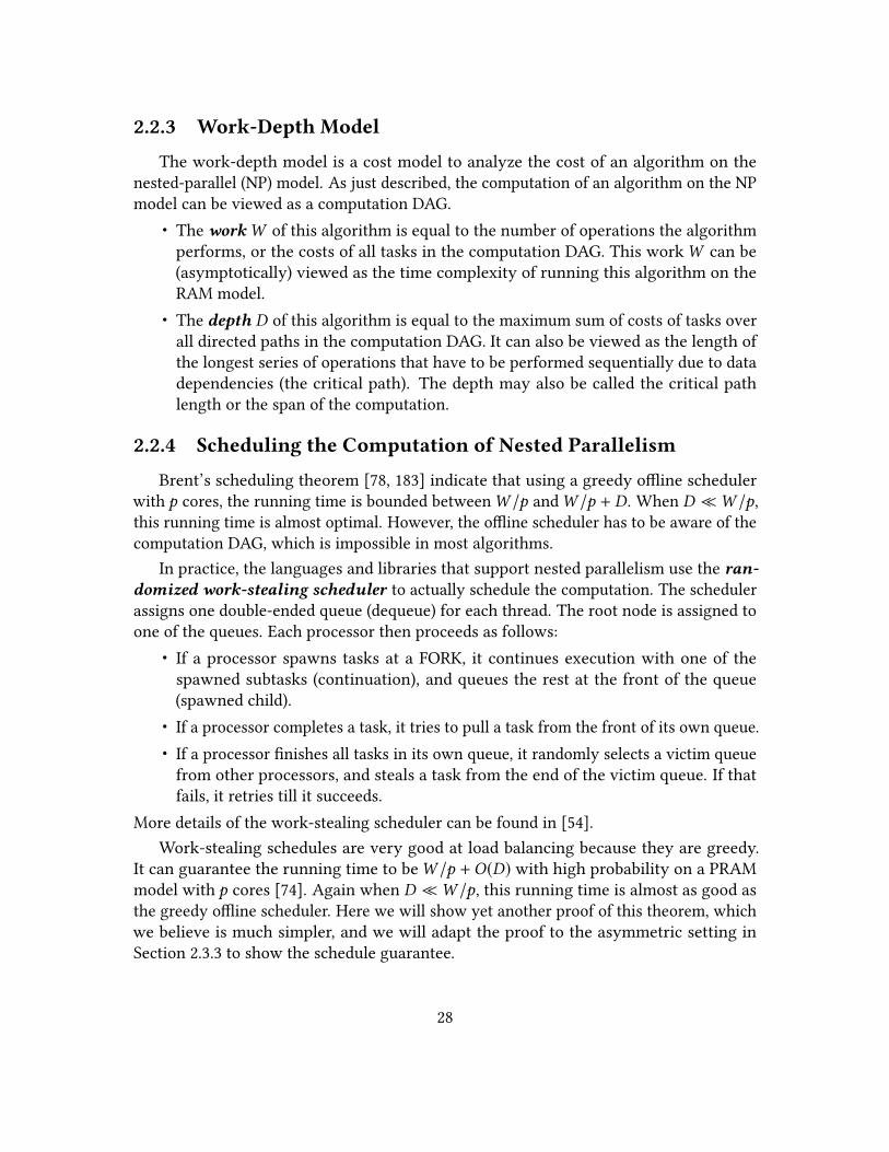
2.2.3 Work-Depth Model

The work-depth model is a cost model to analyze the cost of an algorithm on thenested-parallel (NP) model. As just described, the computation of an algorithm on the NPmodel can be viewed as a computation DAG.

• The workW of this algorithm is equal to the number of operations the algorithmperforms, or the costs of all tasks in the computation DAG. This workW can be(asymptotically) viewed as the time complexity of running this algorithm on theRAM model.

• The depth D of this algorithm is equal to the maximum sum of costs of tasks overall directed paths in the computation DAG. It can also be viewed as the length ofthe longest series of operations that have to be performed sequentially due to datadependencies (the critical path). The depth may also be called the critical pathlength or the span of the computation.

2.2.4 Scheduling the Computation of Nested Parallelism

Brent’s scheduling theorem [78, 183] indicate that using a greedy oine schedulerwith p cores, the running time is bounded betweenW /p andW /p + D. When D W /p,this running time is almost optimal. However, the oine scheduler has to be aware of thecomputation DAG, which is impossible in most algorithms.

In practice, the languages and libraries that support nested parallelism use the ran-domized work-stealing scheduler to actually schedule the computation. The schedulerassigns one double-ended queue (dequeue) for each thread. The root node is assigned toone of the queues. Each processor then proceeds as follows:

• If a processor spawns tasks at a FORK, it continues execution with one of thespawned subtasks (continuation), and queues the rest at the front of the queue(spawned child).

• If a processor completes a task, it tries to pull a task from the front of its own queue.• If a processor nishes all tasks in its own queue, it randomly selects a victim queue

from other processors, and steals a task from the end of the victim queue. If thatfails, it retries till it succeeds.

More details of the work-stealing scheduler can be found in [54].Work-stealing schedules are very good at load balancing because they are greedy.

It can guarantee the running time to beW /p +O(D) with high probability on a PRAMmodel with p cores [74]. Again when D W /p, this running time is almost as good asthe greedy oine scheduler. Here we will show yet another proof of this theorem, whichwe believe is much simpler, and we will adapt the proof to the asymmetric setting inSection 2.3.3 to show the schedule guarantee.

28

Theorem 2.2.1. A work-stealing schedule with p processors on a binary DAG of sizeW anddepth D will take at mostW /p +O(D) time on a CRCW PRAM whp2.

The main step to prove the theorem is show that the overall number of steals for theentire computation is upper bounded by O(pD) whp. This result is of an independentinterest as a step in the proof of Theorem 2.2.1, since such steals are the only schedulingoverhead other than the necessary computation which is captured by the work termWthat we have to pay even sequentially. When a parallel algorithm has a small depth D(e.g., O(polylog(n))), such overhead is always negligible.

To prove the theorem, we rst show the following lemma.

Lemma 2.2.2. It takes O((p − 1)(D + log(1/ϵ)) steals from p − 1 processors to steal D tasksfrom one queue with probability at least 1 − ϵ .

Proof. The most optimistic situation is that, no two steals process in the same timestep(i.e., each steal does not aect each other). In this case, each steal has 1/(p − 1) probabilityto hit the queue and steal one task. The probability that S = 2(p − 1)(D + log(1/ϵ)) stealsincur less than D hits is no more than e−δ

2µ/2 by Cherno bound where µ = 2D+2 log(1/ϵ)and δ = (D + log(1 − ϵ))/µ. Plugging in the values leads to the probability to be less thanϵ .

However, it is possible that multiple steals occur simultaneously in one timestep andonly one of them succeeds while others fail even though they hit the queue. The mostpessimistic situation is that p − 1 steals always happen together, which maximize thechance that a steal hits the queue but fails to get the task since it is taken by anothersimultaneous steal. The possibility that at least one of the p − 1 steals hit the queue in onetimestep (so that at least one of the task is stolen) is at least 1− (1− 1/(p − 1))p−1 > 1− 1/e .

We can then apply a similar analysis to show that the probability that less than D tasksare stolen after S′ = 2(D + log(1/ϵ))/(1 − 1/e) steps is small. Similar to the previous case,such probability is no more than e−δ

2µ/2 by Cherno bound where µ = 2D + 2 log(1/ϵ)and δ = (D + log(1−ϵ))/µ. This gives the same probability of less than ϵ , and S′ timestepscontain (p − 1)S′ = O(p(D + log(1/ϵ))) steals.

With Lemma 2.2.2, we now prove Theorem 2.2.1.Proof of Theorem 2.2.1. We consider each path in the DAG, and show that it can be nishedwith O(pD) steals whp. For each specic path, the length is no more than D. Each nodeon this path is either a spawned child or executed directly after the previous node by thesame processor. We now show that this path can be nished using no more than O(pD)steals. It is easy to see that the later case (i.e., the next node will always be executed inthe next timestep) is strictly better than the rst case when a steal is required to continue

2We say a result holds with high probability (whp) for an input of size n if it holds with probability atleast 1 − n−c , for any constant c > 0, over all possible random choices made by the algorithm.

29

the execution of this path. It is possible that the spawned child is not stolen until thecontinuation nishes and the processor takes over this branch, but this will only help.

As a result, the worst case is when all nodes on the path are spawned children. In thiscase, since we assume that a FORK spawns a task in a unit time, at any synchronized stepthere is always a task available to be stolen. Since the length of the path is no more thanD, Lemma 2.2.2 can upper bound the number of steals to nish the execution of this path(here the D tasks waiting to be stolen may not necessarily in the same queue, but thisdoes not aect the analysis). Given a DAG with depth D, there are at most 2D paths in theDAG, so if we set ϵ = 2D · nc for any constant c ≥ 1, O(p(D + logn)) steals are sucientfor executing all existing paths. We note that since the input size is at least n and theDAG needs to have D = Ω(logn) depth to contains Ω(n) nodes, the logn term will notdominate.

In every timestep, each processor is either making some progress on processing a node,or trying for a steal attempt. The DAG containsW nodes and we have upper boundedthe number of steal attempts. Since we have p processors, the entire computation canbe executed in (W +O(pD))/p =W /p +O(D) time. Namely, other than theW /p term toactually execute the computations in the DAG, O(pD) steals are the upper bound for theadditional cost for the work-stealing scheduler, which is an additional O(D) cost whenexecuting on a p-processor machine.

This proof can be viewed as a simplied version of the previous proofs in [2, 30, 54, 74],and we show how it can be adapted into the asymmetric setting in Section 2.3.2.

Meanwhile, since the scheduler dierentiates between “local” and “remote” work basedon queues, it also preserves locality well, especially if the depth of the program is small.Intuitively, a low-depth program does not present many opportunities for stealing [74]. Ifthe sequential I/O or cache complexity is Q1(n;M,B) with private caches, then the totalnumber of cache misses for all caches Qp(n;M,B) is bounded by Q1(n;M,B) +O(pDM/B)in expectation [2]. On a parallel machine with a share cache, using the parallel depth-rst(PDF) scheduler [57], then Qp(n;M + pMB,B) ≤ Q1(n;M,B). Most parallel algorithmsthroughout this thesis have only polylogarithmic depth, so that the parallel I/O or cachecomplexity is asymptotically bounded by Q1, when plugging in the parameters from thereal-world settings. As a result, it is usually enough to just analyze the sequential I/O orcache complexity, and the overhead caused by parallelism is negligible.

2.3 Models Accounting for Asymmetry

In Section 2.1 we reviewed the existing computational models that not only measurethe costs of computations, memory access, and parallelism of an algorithm, but alsoprovide an objective to optimize when designing algorithms for a specic problem. Thesecost models are therefore heavily used in algorithm research and conducting practicalimplementations. Unfortunately, none of these models have considered the asymmetric

30

cost between reads and writes, so directly applying algorithms designed to optimizethe existing measurements may not be ecient on the future hardware. We will nowintroduce how these models can be extended to the asymmetric setting.

2.3.1 (M,ω)-Asymmetric RAM: the Sequential Model

To start with, the rst machine model that will be introduced is the (M,ω)-AsymmetricRAM, which is used to analyze the sequential costs of computations, memory access.

Similar to the external-memory and cache-oblivious model, (M,ω)-ARAM assumes asymmetric small-memory of size M ≥ 1 3, an asymmetric large-memory of unboundedsize, and a write cost ω ≥ 1, which is assumed to be an integer without loss of generality.Typically, we are interested in the setting where n M , where n is the input size, andω 1.

Table 2.2: The cost of a single access to the two memories for ARAM cost and work on (M,ω)-ARAM.

Measure small-memory large-memory

ARAM cost Q 0 read: 1, write: ωworkW 1 read: 1, write: ω

The model assumes standard random access machine (RAM) instructions. Two costmeasures for computations are considered in the model. The (asymmetric) ARAM cost Qis dened as the total number of reads from large-memory plus ω times the number ofwrites to large-memory. The (asymmetric) workW is dened as the ARAM cost plus thenumber of reads from and writes to small-memory.4 Because all instructions are frommemory, this includes any cost of computation. In the thesis, the results are presentedusing both cost measures.

The model contrasts with the external-memory model [7] in the asymmetry of theread and write costs. For simplicity, as the very rst research on write-ecient algorithms,the simple version of the memory is not partitioned into blocks of size B to keep thealgorithms simpler. It is worth to mention that even the case of M = O(1) is interesting.An example of this is the asymmetric sorting algorithms introduced in Section 4.4.1.

This blocking can easily be considered if necessary. In this case each read/writeloads/stores a memory block of B words. This is referred to the (M,B,ω)-ARAM. Weonly measure the ARAM cost Q on this model since it seems unreasonable to dene the

3The small-memory contains M words, each of size Θ(logn) for input size n.4The work metric models the fact that reads to certain emerging asymmetric memories are projected to

be roughly as fast as reads to symmetric memory (DRAM). The ARAM cost metric Q does not make thisassumption and hence is more generally applicable.

31

corresponding work when considering this block size. An example of algorithms analyzedusing the (M,B,ω)-ARAM is given in Section 4.4.3.

The workW in the (M,ω)-ARAM is the analogy of the time complexity of the sym-metric case. Each basic operation or a read is also counted as a unit cost, and a write tothe large-memory costs ω. Since there is usually a return value for each operation, thesmall-memory is necessary in the asymmetric setting (otherwise each operation will costω). Here the reason we use the word “work” instead of “time” is to be consistent with theparallel setting.

2.3.2 Asymmetric NP Model: the Parallel Model

We now introduce the cost model of nested-parallel computations. The model is namedas the Asymmetric Nested-Parallel (NP) model and can be viewed as the asymmetricextension of the nested-parallel model.

The Asymmetric Nested-Parallel (NP) model assumes a stack allocated symmetricsmall-memory, and a heap allocated asymmetric large-memory. Stack allocated memoryis memory allocated by a task, available to the task and its children, but invalid whenthe task nishes. Heap allocated memory is allocated by a task and can be accessedby any other task, including ancestor tasks (it is completely shared memory). Eachinstruction has weight one, except a write to the heap memory, which has weight ω ≥ 1(in practice, ω 1). When analyzing an algorithm, the term “writes” will be used torefer to the number of writes to heap allocated memory. We assume the amount of stackmemory allocated by all but the leaf tasks (tasks with no forks) is constant. The amountof symmetric stack memory a leaf task can allocate is bounded by a parameter Ml . Thisseparation into stack and heap allocated memory, and the distinction between leaf andnon-leaf tasks for stack memory size, is made both because it is a convenient model forusing the dierent memories, and also because it enables an ecient mapping onto a xednumber of processors, as justied below.

Note that the Asymmetric NP is an algorithmic cost model, as opposed to a machinemodel, enabling reasoning about nested-parallel computations without worrying aboutmapping the computation to machines. We address this scheduling issue next.

2.3.3 Scheduling Asymmetric NP Computations

This section shows that the algorithmic cost metrics of Asymmetric NP are sucientlydescriptive to capture the performance of Asymmetric NP computations when using goodschedulers.

The Asymmetric NP model has been designed in a manner that yields an ecientmapping to an (M,ω)-Asymmetric PRAM machine model. In this model, there are pprocessors, each running its own instructions using a small symmetric local memoryof size M . The processors share an unbounded asymmetric global memory, to which

32

concurrent reads and writes are allowed. We also allow any processor to read the localmemory of another processor (concurrently), but not to write to it. A request to readthe local memory of another processor is viewed as requiring a write out to the globalmemory in order to enable the read, and hence is charged ω. On each processor anywrite to the global memory also takes ω time. All other instructions take unit time. Forsynchronizing we assume an atomic fetch-and-add to the global memory that can beperformed in constant depth and work linear in the number of processors.

The challenge with Asymmetric NP computations is that stack variables must bewritten out to global memory before tasks can be migrated to a dierent processor fromthe one that forked it. The naïve approach would forego the stack and instead write allO(1) stack variables for non-leaf tasks directly to global memory, making each FORKcost Θ(ω). For ne-grained parallelism especially, where the number of FORKs for analgorithm with workW is Ω(W ), this approach would yield running time no better thanΩ(ωW /p). In other words, one may as well consider every instruction a write if adoptingthe naïve scheduler.

Here we show that a variant of a work-stealing scheduler [74] achievesW /p +O(ωD)expected time when limited to binary forking. As discussed in Section 2.2.4, in standard(symmetric-memory) work stealing, each worker (or processor) maintains a double-endedqueue called a deque of tasks that are ready to execute. Whenever a worker executesa (binary) FORK instruction, the processor continues working on the “left” child taskand places the “right” child on the bottom of its deque. When a worker completes atask by executing its FINISH instruction, there are two options. If that task enabledanother one, i.e., the completed task was the last outstanding child of its parent, then theworker continues working on the now-enabled parent. Otherwise, the worker removesthe bottom task from its deque and executes it. If the deque is empty, the worker insteadsteals, meaning that it chooses a random victim processor and takes the task from thetop of that processor’s deque if the deque is non-empty. In the event that the steal isunsuccessful, the worker will continue to attempt to steal until it successfully steals a taskor the computation is nished.

In the Asymmetric NP model, working locally on a deque is cheap, and in general stackframes need not be written out. For example, if the entire computation runs sequentiallyon one processor, then no stack-related writes occur (assuming that the local memory islarge enough to hold the stack depth).

There are still some challenges, however, most notably on steals. Because a task hasaccess to any stack variables of its ancestor tasks, any unwritten stacks of ancestor tasksmust be written out to global memory when a steal occurs. This situation is particularlychallenging to analyze as it may cause steals to take time proportional to ω times thenesting depth. To cope with this challenge, Lemma 2.3.1 shows that a simple modicationto work stealing results in at most a constant number of frames needing to be written. Weassume that a steal request somehow interrupts its target task (e.g., all tasks can regularly

33

poll to check if there are any outstanding steal requests), and if work is available, theregisters for the stolen task and relevant ancestors are written to the asymmetric globalmemory. There is a similar potential issue when a task completes: its return value mustbe written to its parent task, which may no longer be local, and hence a write to globalmemory could be required.

Lemma 2.3.1. There exists a variant of work stealing such that on each steal (or stealattempt), only O(1) stack frames are written to global memory.

Proof. The lemma can be achieved either by modifying work stealing or by an equivalentprogram transformation. The program transformation is as follows. Transform everyFORK into two FORKs as follows. First FORK two tasks: the left child performs theintended FORK, which we call a forking task, and the right child is a dummy task thatdoes nothing. The dummy task is inserted onto the deque, whereas the worker continuesto execute the forking task. (In Cilk-like work-stealing, e.g., [74], expressing the FORK astwo “spawns” followed by a “sync” would automatically create a similar dummy task as acontinuation from the second spawn.)

We claim that for the topmost task on the deque (i.e., the one that can be stolen), atmost its parent and grandparent have not already been written out to global memory.In order for a task to be on the deque and hence stealable, it must be the right child ofits parent. A simple induction shows that for any task on a deque, all right children ofancestors have either been stolen already or are on the same deque. (A similar claim isproven as Lemma 3 in [30].) Thus, a steal need only write-out the frames corresponding tothe longest right-only path in the computation graph. The longest is three nodes, whichwe can show by cases. A forking task is always the left child and hence not stealable. Areal task (i.e., one existing before the transformation) is always the child of a forking task,so it can have at most one unwritten ancestor frame: the parent forking task. A dummytask is always the right child of a real task, so stealing a dummy task could entail writingout three frames.

Theorem2.3.2. Consider a computation in the Asymmetric NPmodel with binary branchingfactor,W work, D unweighted depth, δ nesting depth, andMl leaf stack memory. There existsa work-stealing scheduler that executes the computation inW /p +O(ωD) expected time ona p-processor (O(δ ) +Ml ,ω)-Asymmetric PRAM.

Proof. Our analysis is based on the proof of Theorem 2.2.1. But we need to account forthe fact that (1) steals involve writing out to global memory, and (2) nishing tasks mayalso entail writing out to global memory, i.e., if the parent frame is in global memory.

We will use the similar argument from Section 2.2.4 that at most O(pD) steals aresucient for the entire computation. Note that based on our assumption and Lemma 2.3.1,each successful steal occupies two processors for at most O(ω) timesteps during the stealprocess and the join part, since a constant stack frames are required to communicate viathe global memory.

34

To adapt the analysis for Lemma 2.2.2 and Theorem 2.2.1, we now require a processorto idle for t = Θ(ω) timesteps after each unsuccessful steal, before the next steal attempt.By making this change, each successful steal can only “block” at most O(p) simultaneoussteal attempts instead of O(ωp) steal attemps. Therefore, the proof of Lemma 2.2.2 andTheorem 2.2.1 with minor modications can adapt to here.

For a path in this setting, each node is either a FORK operation, which is local andassumed to use unit time, or a regular instruction which requires either unit time or ωtime when it is write to the shared asymmetric large-memory. The path can always makeprogress on the same processor, unless the nodes that are spawn children that need to bestolen. Since the (unweighted) length of the path is upper bounded by D and the stealattempts from one processor appear at most once in every O(ω) timesteps, we can showthat for every O(ω) timesteps, we can either proceed at least one step further on thepath (corresponding to nodes that are not spawn children), or there is at least an taskcorresponding to a spawn children available to be stolen in the deque. Since there are atmost D spawn children on one path, O(pD) steals are sucient to nish the computationon all paths in the DAG. The analysis in Lemma 2.2.2 and Theorem 2.2.1 can directly gothrough and the only dierence is that at most O(p) instead of p − 1 steals can aect eachother, but such dierence only inuence the constant in the big-O. Other than the writesto the asymmetric large-memory during the steal, assuming local small-memory is largeenough to hold the entire stack (i.e., O(δ ) +Ml )), the only additional writes that occur arewhen a child returns to a parent task that resides in large-memory, i.e., it has been stolen.This event also requires writes to the asymmetric large-memory, but the number of thesewrites is bounded by the number of steals.

Since we can bound the number of steals to be O(pD) and each steal costs O(ω), wethus have a total running time that isW /p +O(ωS/p) =W /p +O(ωD).

In a very high level, each steal attempt is slowed down and charged for O(ω) timeinstead of a unit time. Despite that a steal is more expensive, less frequent steal is overallbenecial (each processor can execute more work) and will not increase the number ofsteals.

The above theorem provides justication for charging only unit cost for FORK, andfor example, means that the standard reduce via a binary tree incurs only Θ(n + ω) workinstead of Θ(ωn) work on the Asymmetric NP, as discussed in Section 4.2. Note also thatour separate accounting for leaf stack memory in the Asymmetric NP model, and theobservation that the non-leaf tasks of all the algorithms in this thesis each allocate onlyO(1) stack memory, means that the bound in the lemma is only a constant number ofwrites per steal, whereas without the separate accounting, it would be O(Ml ) writes persteal.

Bulk-Synchronous Computations.

35

Many of the algorithms in this thesis are bulk-synchronous algorithms for whichthere is only one level of nesting (δ = 1). The root task proceeds in a sequence of R rounds.In each round i it forks ni child tasks (each a leaf) and waits for them to nish. The roottask can run arbitrary computation between such rounds. We dene the iteration count Ias

∑Ri=1 ni . The following lemma for scheduling bulk-synchronous algorithms provides

additional support for the model.

Lemma 2.3.3. A bulk-synchronous computation with arbitrary branching on the Asym-metric NP model with W work, D (unweighted) depth, I iteration count, and Ml leafstack memory, can be simulated on an (O(Ml ),ω)-Asymmetric PRAM with P processorsin O((W + ωI )/p + ωD) time.

Proof. The idea is that the root task runs on some processor and when it gets to a fork,it sets up the registers for the children and sets a count to n. The processors then grabtasks by decrementing this count (using the fetch-and-add). When the count reaches zeroidle processors quit for that round and wait for a later round when it is again set to somenon-zero number. A separate counter can be used to detect when all processors are done,and the processor that detects termination can continue with the root task. The additionalwork done for accessing the counter is O(ωI ) and most pessimistically the charge to theweighted depth is O(ωD) so using Brent’s scheduling principle [78], (T ≤W /p + D), wehave the given time bounds.

Each child task takes O(Ml ) local memory. Since the nesting depth is one, the totalmemory needed by a child task is O(Ml + 1). This gives the memory bound.

We note that in the realistic cases, each leaf task needs at least a write after thecomputation, so the ωI term will not dominate. As a result, even with a slightly dierentdenitions for workW and depth D in the bulk-synchronous computation, we do notspecically identify this case in the rest of this thesis since the simulated running time isthe same as O(W /p + ωD).

2.3.4 Asymmetric Ideal-Cache Model and Cache Policy

Recall from Section 2.1.3 the Ideal-Cache model [131] is a variant of the external-memory model. The machine model is organized in the same way with two memorieseach partitioned into blocks, but there are no explicit memory transfer instructions. Insteadall addressable memory is in the large-memory, but any subset of up to M/B of the blockscan have a copy resident in the small-memory (cache). Any reference to a resident blockis a cache hit and is free. Any reference to a word in a block that is not resident is acache miss and requires a memory transfer from the large-memory. The cache miss canreplace a block in the cache with the loaded block, which might require evicting a cacheblock. The model makes the tall cache assumption where M = Ω(B2), which is easily metin practice. The I/O or cache complexity of an algorithm is the number of cache misses.An optimal (oine) cache eviction policy is assumed—i.e., one that minimizes the I/O

36

complexity. It is well known that the optimal policy can be approximated using the onlineleast recently used (LRU) policy at a cost of at most doubling the number of misses, anddoubling the cache size [257].

The main purpose of the Ideal-Cache model is for the design of cache-oblivious algo-rithms. These are algorithms that do not use the parameters M and B in their design, butfor which one can still derive eective bounds on I/O complexity. This has the advantagethat the algorithms work well for any cache sizes on any cache hierarchies. The I/Ocomplexity of cache-oblivious sorting is asymptotically the same as for the EM model.

In order to distinguish the extra cost of writes from reads, the Asymmetric Ideal-Cache model is dened as follows. A cache block is dirty if the version in the cache hasbeen modied since it was brought into the cache, and clean otherwise. When a cachemiss evicts a clean block the cost is 1, but when evicting a dirty block the cost is 1 + ω,1 for the read and ω for the write. Again, we assume an ideal oine cache replacementpolicy—i.e., minimizing the total I/O cost.

Under this model however, we note that the LRU policy is no longer 2-competitivecomparing to the optimal oine policy. Consider a cache with k = M/B blocks and amemory access pattern that repeatedly and sequentially writes to k − 1 blocks and readfrom other k − 1 blocks. An ideal cache policy will keep all k − 1 blocks associated towrites, so the I/O cost of each round is k − 1 for k − 1 read misses. An LRU policy howevercauses a cache miss for every single memory access, leading the I/O cost of each round toω(k − 1)+k − 1. This approximation is proportional to ω, which is problematic. Thereforea new variant of the cache replacement policy is required, which needs to be competitivewithin a constant factor.

The idea is to separately maintain two equal-sized pools of blocks in the cache (primarymemory), a read pool and a write pool. When reading a location, (i) if its block is in theread pool we just read the value; (ii) if it is in the write pool we copy the block to the readpool; or (iii) if it is in neither, we read the block from secondary memory into the readpool. In the latter two cases we evict the LRU block from the read pool if it is full, withcost 1. The rules for the write pool are symmetric when writing to a memory location,but the eviction has cost ω + 1 because the block is dirty. We call this the read-write LRUpolicy. This policy is competitive with the optimal oine policy:

Lemma 2.3.4. For any sequence S of instructions, if it has cost QI (S) on the AsymmetricIdeal-Cache model with cache sizeMI , then it will have cost

QL(S) ≤ML

ML −MIQI (S) + (1 + ω)MI/B

on an asymmetric cache with read-write LRU policy and cache sizes (read and write pools)ML.

Proof. Partition the sequence of instructions into regions that contain memory reads toexactly ML/B distinct memory blocks each (except perhaps the last). Each region will

37

require at most ML/B misses under LRU. Each will also require at least (ML −MI )/B cachemisses on the ideal cache since at most MI/B blocks can be in the cache at the start ofthe region. The same argument can be made for writes, but in this case each operationinvolves evicting a dirty block. The (1 + ω)MI/B is for the last region. To account for thelast region, in the worst case at the start of the last write region the ideal cache starts withMI/B blocks which get written to, while the LRU starts with none of those blocks. TheLRU therefore invokes an addition MI/B write misses each costing 1 + ω (1 for the loadand ω for the eviction). Note that if the cache starts empty then we do not have to addthis term since an equal amount will be saved in the rst round.

We dene the asymmetric I/O cost or asymmetric cache complexity to be the costof an algorithm on the asymmetric ideal-cache model.

2.3.5 Asymmetric Low-depth Cache-Oblivious Paradigm

The last model considered in this thesis is based on developing low-depth cache-oblivious algorithms [58]. As discussed in Section 2.1.3, the cache complexity can beanalyzed on the Ideal-Cache model under this sequential order.

Using known scheduling results the depth and sequential cache complexity of acomputation are sucient for deriving bounds on parallel cache complexity. In particular,let D be the depth and Q1 be the sequential cache complexity. Then for a p-processorshared-memory machine with private caches (each processor has its own cache) using awork-stealing scheduler, the total number of misses Qp across all processors is at mostQ1+O(pDM/B)with high probability [2]. For ap-processor shared-memory machine witha shared cache of size M + pBD using a parallel-depth-rst (PDF) scheduler, Qp ≤ Q1 [50].These bounds can be extended to multi-level hierarchies of private or shared caches,respectively [58]. Thus, algorithms with low depth have good parallel cache complexity.

The asymmetric variant of the low-depth cache-oblivious paradigm simply accountsfor ω in the depth and uses the Asymmetric Ideal-Cache model for sequential cachecomplexity. We observe that the above scheduler bounds readily extend to this asymmetricsetting. The O(pDM/B) bound on the additional cache misses under work-stealing arisesfrom anO(pD) bound on the number of steals and the observation that each steal requiresthe stealer to incur O(M/B) misses to “warm up” its cache. Pessimistically, we will charge2M/B writes (and reads) for each steal, because each line may be dirty and need writingback before the stealer can read it into its cache and, once the stealer has completed thestolen work (reached the join corresponding to the fork that spawned the stolen work),the contents of its cache may need to be written back. Therefore for private caches wehave QP ≤ Q1 +O(ωpDM/B). The PDF bounds extend because there are no additionalcache misses and hence no additional reads or writes.

38

Chapter 3

Lower Bounds

We start by showing a variety of lower bounds on (M,ω)-ARAM of some fundamen-tal problems including Fast Fourier Transform (FFT), sorting network, diamond DAGs,permuting and sorting. These lower bounds mainly focus on the number of I/Os to thelarge-memory (i.e., the ARAM cost). From a theoretical point of view, these lower boundsindicate the amount of improvement that can be made to the classic algorithms withoutconsidering the asymmetry between reads and writes. That further leads us to designalgorithms that are asymptotically optimal on (M,ω)-ARAM and close the gaps. On theother hand, these lower bounds show the hardness of these problems, indicating thatpractically (i.e., considering the actual values of ω and M), we can only achieve a constantimprovement unless M = o(ω), which seems to be unrealistic. A list of results are shownin Table 3.1.

In a high-level overview, we show that FFT and sorting network that have xed com-putational DAG, the amount of improvement is limited to log(ωM)/logM (the previousbounds are listed in Table 2.1 and B = 1). For Diamond DAG the result is interesting: weshow that there is no asymptotic improvement without allowing redundant computation,even if the reads are free! The proof techniques are to partition a computation into sub-computations that each have a lower bound on cost, but an upper bound on the numberof inputs and outputs, which lower bound the costs to nish the computations of theseproblems.

Based on the model proposed in this thesis, Jacob and Sitchinava [182] recently showthe lower bounds on permuting, sorting and sparse-matrix vector multiplication, and theresults are also summarized in Table 3.1. In this case the block size B is also consideredsince the bounds are trivial otherwise. The outline of these results are overviewed inSection 3.5.

39

(a). The results in this thesis based on the (M,ω)-ARAM.

Problems ARAM Cost (Q) Work (W ) Remarks

FFT Q(n) = Ω

(ωn lognlog(ωM)

)W (n) = Q(n) + Ω(n logn) Section 3.2

Sorting Network Q(n) = Ω

(ωn lognlog(ωM)

)W (n) = Q(n) + Ω(n logn) Section 3.3

Diamond DAG Q(n) = Ω

(ωn2

M

)W (n) = Q(n) + Ω(n2) Section 3.4

(b). Later results from Jacob and Sitchinava’s 2017 SPAA paper based on the (M,B,ω)-ARAM. Onthese problems, the block size B (full denition given in Section 2.1.2) is considered since the

bounds are trivial otherwise.

Problems ARAM Cost (Q) Remarks

Permuting and sorting Q(n) = Ω

(min

n,

ωn log(n/B)B log(ωM/B)

)Section 3.5

SparseMxV Q(n) = Ω

(min

h,ωh log(n /maxh/n,M)

B log(ωM/B)

)Section 3.5

Table 3.1: Summary of lower bounds on the (M,ω)-ARAM. In all cases n is the input size. Insparse-matrix vector multiplication (referred to as “SparseMxV” in the table), h is the number ofnon-zero elements in the matrix.

3.1 General Technique in the Proofs

To start with, we show the general techniques to show the lower bounds for FastFourier Transform (FFT) DAGs, sorting networks and diamond DAGs. The idea in showingthe lower bounds is to partition a computation into subcomputations that each have alower bound on cost, but an upper bound on the number of inputs and outputs they canuse. Our lower bound for FFT DAGs then uses an interesting accounting technique thatgives every node in the DAG a unit weight, and fractionally assigns this weight acrossthe subcomputations. In the special case ω = 1, this leads to a simpler proof for the lowerbound on the I/O complexity of FFT DAGs than the well-known bound by Hong andKung [170].

We refer to a subcomputation as any contiguous sequence of instructions. The outputsof a subcomputation are the values written by the subcomputation that are either anoutput of the full computation or read by a later subcomputation. Symmetrically, theinputs of a subcomputation are the values read by the subcomputation that are either

40

Figure 3.1: An example of the com-putational DAG of a FFT DAG (aka.buttery networks) of size 8. The ver-tices in top row are the input and thebottom row is the output. This net-work has 3 levels, and in each leveleach vertex depends on the its ownvalue in the previous level, as well asthe vertex with index that reverses thei-th bit, where i is the number of level.

an input of the full computation or written by a previous subcomputation. The spaceof a computation or subcomputation is the number of memory locations both read andwritten. An (l,m)-partitioning of a computation is a partitioning of instructions intosubcomputations such that each has at most l inputs and at mostm outputs. We allow forrecomputation—instructions in dierent subcomputations might compute the same value.

Lemma 3.1.1. Any computation in the (M,ω)-ARAM has an ((ω + 1)M, 2M)-partitioningsuch that at most one of the subcomputations has ARAM cost Q < ωM .

Proof. We generate the partitioning constructively. Starting at the beginning, partitionthe instructions into contiguous blocks such that all but possibly the last block has costQ ≥ ωM , but removing the last instruction from the block would have cost Q < ωM . Toremain within the cost bound each such subcomputation can read at mostωM values fromlarge-memory. It can also read the at most M values that are in the small-memory whenthe subcomputation starts. Therefore it can read at most (ω + 1)M distinct values fromthe input or from previous subcomputations. Similarly, each subcomputation can writeat most M values to large-memory, and an additional M that remain in small-memorywhen the subcomputation ends. Therefore it can write at most 2M distinct values that areavailable to later subcomputations or the output.

3.2 Fast Fourier Transform (FFT)

We now consider lower bounds for the DAG computation problem for the family ofFFT DAGs (also called FFT networks, or buttery networks). The FFT DAG of input sizen = 2k consists of k + 1 levels each with n vertices (total of n log 2n vertices). Each vertex(i, j) at level i ∈ 0, . . . ,k − 1 and row j has two out edges, which go to vertices (i + 1, j)and (i + 1, j ⊕ 2i) (⊕ is the exclusive-or of the bit representation). An example of suchDAG with n = 8 is shown in Figure 3.1. This is the DAG used by the standard FFT (FastFourier Transform) computation. We note that in the FFT DAG there is at most a singlepath from any vertex to another.

41

Lemma 3.2.1. Any (l,m)-partitioning of a computation for simulating an n input FFT DAGhas at least n logn/(m log l) subcomputations.

Proof. We refer to all vertices whose values are outputs of any subcomputation, as partitionoutput vertices. We assign each such vertex arbitrarily to one of the subcomputations forwhich it is an output.

Consider the following accounting scheme for fractionally assigning a unit weight foreach non-input vertex to some set of partition output vertices. If a vertex is a partitionoutput vertex, then assign the weight to itself. Otherwise take the weight, divide it evenlybetween its two immediate descendants (out edges) in the FFT DAG, and recursivelyassign that weight to each. For example, for a vertex x that is not a partition outputvertex, if an immediate descendant y is a partition output vertex, then y gets a weight of1/2 from x , but if not and one of y’s immediate descendants z is, then z gets a weight of1/4 from x . Since each non-input vertex is fully assigned across some partition outputvertices, the sum of the weights assigned across the partition output vertices exactlyequals |V | − n = n logn. We now argue that every partition output vertex can have atmost log l weight assigned to it. Looking back from an output vertex we see a binarytree rooted at the output. If we follow each branch of the tree until we reach an inputfor the subcomputation, we get a tree with at most l leaves, since there are at most linputs and at most a single path from every vertex to the output. The contribution ofeach vertex in the tree to the output is 1/2i , where i is its depth (the root is depth 0). Theleaves (subcomputation inputs) are not included since they are partition output verticesthemselves, or inputs to the whole computation, which we have excluded. By inductionon the tree structure, the weight of that tree is maximized when it is perfectly balanced,which gives a total weight of log l .

Therefore since every subcomputation can have at mostm outputs, the total weightassigned to each subcomputation is at most m log l . Since the total weight across allsubcomputations isn logn, the total number of subcomputations is at leastn logn/(m log l).

Theorem 3.2.2 (FFT Lower Bound). Any solution to the DAG computation problem on

the family of FFT DAGs parametrized by input size n has costs Q(n) = Ω

(ωn lognlog(ωM)

)and

W (n) = Ω(Q(n) + n logn) on the (M,ω)-ARAM.

Proof. By Lemma 3.1.1 every computation must have an ((ω + 1)M, 2M)-partitioning withsubcomputation cost Q ≥ ωM (except perhaps one). Plugging in Lemma 3.2.1 we haveQ(n) ≥ ωMn logn/(2M log((ω + 1)M)), which gives our bound on Q(n). ForW (n) we justadd in the cost of the computation of each vertex.

Note that whichever of ω and M is larger will dominate in the denominator of Q(n).Whenω ≤ M , these lower bounds match those for the standard external memory model [7,

42

170] assuming both reads and writes have cost ω. This implies that cheaper reads do nothelp asymptotically in this case. When ω > M , however, there is a potential asymptoticadvantage for the cheaper reads.

3.3 Sorting Networks

A sorting network is a acyclic network of comparators, each of which takes two inputkeys and returns the minimum of the keys on one output, and the maximum on the other.For a family of sorting networks parametrized by n, each network takes n inputs, has nordered outputs, and when propagating the inputs to the outputs must place the keys insorted order on the outputs. A sorting network can be modeled as a DAG in the obviousway. Ajtai, Komlós and Szemerédi [12] described a family of sorting networks that havesize O(n logn) and depth O(logn). Their algorithm is complicated and the constants arevery large. Many simplications and constant factor improvements have been made,including the well known Patterson variant [227] and a simplication by Seiferas [250].Recently Goodrich [148] gave a much simpler construction of an O(n logn) size network,but it requires polynomial depth. Here we show lower bounds of simulating any sortingnetwork on the (M,ω)-ARAM.

Theorem3.3.1 (Sorting Lower Bound). Simulating any family of sorting networks parametrized

on input sizen hasQ(n) = Ω

(ωn lognlog(ωM)

)andW (n) = Ω(Q(n)+n logn) on the (M,ω)-ARAM.

Proof. Consider an (l,m)-partitioning of the computation. Each subcomputation has atmost l inputs from the network, and m outputs for the network. The computation isoblivious to the values in the network (it can only place the min and max on the outputsof each comparator). Therefore locations of the inputs and outputs are xed independentof input values. The total number of choices the subcomputation has is therefore

( lm

)m! =

l !/(l −m)! < lm. Since there are n! possible permutations, we have that the number ofsubcomputations k must satisfy (lm)k ≥ n!. Taking logs of both sides, rearranging, andusing Stirling’s formula we have k > log(n!)/(m log l) > 1

2n logn/(m log l) (for n > e2). ByLemma 3.1.1 we have Q(n) > ωM 1

2n logn/(2M log((1+ω)M)) = 14ωn logn/log((1+ω)M)

(for n > e2).

These bounds are the same as for simulating an FFT DAG, and, as with FFTs, theyindicate that faster reads do not asymptotically aect the lower bound unless ω > M .These lower bounds rely on the sort being done on a network, and in particular that thelocation of all read and writes are oblivious to the data itself. As discussed in the nextsection, for general comparison sorting algorithms, we can get better upper bounds thanindicated by these lower bounds.

43

Figure 3.2: An example of the computationalDAG of a diamond DAG in a 5×5 grid. The valuesin the circles need to be computed. The valuesin the left column and top row can be directlycomputed from the input, and each other valuedepends on its top, left, and top-left neighbors.The bottom-right value is the output.

3.4 Diamond DAG

We consider the family of diamond DAGs parametrized on size n. Each DAG has n2

vertices arranged in a n×n grid such that every vertex (i, j), 0 ≤ i < (n−1), 0 ≤ j < (n−1)has two out-edges to (i + 1, j) and (i, j + 1). The DAG has one input at (0, 0) and oneoutput at (n − 1,n − 1). The family of 3-diamond DAGs additionally have edges from (i, j)to (i + 1, j + 1). An example of such diamond DAG is given in Figure 3.2 as an example.Diamond DAGs have many applications in dynamic programs, such as for the edit distance(ED), longest common subsequence (LCS), and optimal sequence alignment problems.

Lemma 3.4.1 (Cook and Sethi, 1976). Solving the DAG computation problem on the familyof diamond DAGs of input parameter n (size n × n) requires n space to store vertex valuesfrom the DAG.

Proof. Cook and Sethi [106] show that evaluating the top half of a diamond DAG (i + j ≥n − 1) , which they call a pyramid DAG, requires n space to store partial results. Sinceall paths of the diamond DAG must go through the top half, it follows for the diamondDAG.

Theorem 3.4.2 (Diamond DAG Lower Bound). The family of diamond DAGs parametrized

on input size n has Q(n) = Ω

(ωn2

M

)andW (n) = Ω(Q(n) + n2) on the (M,ω)-ARAM.

Proof. Consider the sub-DAG induced by a 2M × 2M diamond (a ≤ i < a + 2M,b ≤ j <b + 2M) of vertices. By Lemma 3.4.1 any subcomputation that computes the last outputvertex of the sub-DAG requires 2M memory to store values from the diamond. The extrain-edges along two sides and out-edges along the other two can only make the problemharder. Half of the 2M required memory can be from small-memory, so the remaining Mmust require writing those values to large-memory. Therefore every 2M × 2M diamondrequires M writes of values within the diamond. Partitioning the full diamond DAG into

44

2M × 2M sub-diamonds, gives us n2/(2M)2 partitions. Therefore the total number of

writes is at least M ×n2

(2M)2=

n2

4M, each with cost ω. For the work we need to add the n2

calculations for all vertex values.

This lower bound is asymptotically tight since a diamond DAG can be evaluated withmatching upper bounds by evaluating each M/2 ×M/2 diamond sub-DAG as a subcom-putation with M inputs, outputs and memory.

These bounds show that for the DAG computation problem on the family of diamondDAGs there is no asymptotic advantage of having cheaper reads. In Section 4.5 we showthat for the ED and LCS problems (normally thought of as a diamond DAG computation), itis possible to do better than the lower bounds. This requires breaking the DAG computationrule by partially computing the values of each vertex before all inputs are ready. Thelower bounds are interesting since they show that improving asymptotic performancewith cheaper reads requires breaking the DAG computation rules.

3.5 Results from Jacob and Sitchinava

Jacob and Sitchinava [182] recently show the lower bounds on permuting, sortingand sparse-matrix vector multiplication, and the results are summarized in Table 3.1. Inthis series of work, the block size B is considered as a non-constant since the bounds aretrivial otherwise. Here we briey overview the outline of their proofs.

The key challenges here is that we no longer have a xed computational DAG. Also,the same cost can be incurred by dierent combinations of reads and writes. To solve this,the proof analyzes batch reads or writes (referred to a “round”) such that the total ARAMcost of each round is at least ωM/B, and the small-memory needs to be emptied betweenrounds.

The proof on permuting is based on a counting argument. This also gives the a lowerbound on sorting consequently since sorting is strictly harder.

Assume any algorithm requires R rounds to nish. The algorithm must distinguish alln! possible inputs, leading to

n!B!n/B

≤ P(R) ≤

((n

ωM/B

) (ωM

M

)2M

M!B!M/B

(3N )M/B)R

P(R) represents the number of “block-wise” permutations that can be generated afterR rounds. On the right of the inequality,

( nωM/B

)is the number of choices of ωM/B blocks

to read out of the inputs.(ωMM

)2M is the number of ways to choose up to M items to keep in

the memory out of the ωM reads from previous. Then block-wisely permuting M items inthe small-memory has M!/(B!M/B) cases. Finally since the memory are emptied betweenrounds, we can write back the M/B blocks into the large-memory with cost ωM/B, and

45

the number of options is no more than (3N )M/B . The whole term on the right side upperbounds the number of permutations that can be identied after R rounds.

For the left term, n! is the number of inputs that the algorithm needs to identify, whileB!n/B is the number of permutations that one block can add up to. This lower boundsthe number of the block-wise permutations that have to be distinguished by a permutingalgorithm.

Solving this inequation gives the lower bound of R. Since the ARAM cost of each roundis at leastωM/B, the lower bound of permuting and sorting is thus Ω(minn,ωn/B logωM/B n/B).

A lower bound on computing the product of a sparse matrix by a dense vector canbe analyzed similarly, using the round-based computation and counting argument. Thebound is listed in Table 3.1. The full details of the proof techniques in this section arereferred to [182].

46

Chapter 4

Basic Algorithmic Building Blocks

To start the write-ecient algorithms, we rst introduce the basic building blocks that arewidely used in designing other algorithms. Therefore, when designing more complicatedand advanced algorithms, these building blocks can be directly used, just like in thesymmetric setting.

We start by showing that a variety of algorithms that are reasonably easy and optimalin Section 4.1. These algorithms include fast Fourier transform (FFT), search trees andpriority queues, and sorting. Some other algorithms like BFS/DFS or planar convex hulland Delaunay triangulation will be described later in the corresponding chapters.

Then later in Section 4.2 and 4.3, we discuss four commonly-used parallel primitives,i.e., reduce, lter, list and tree contractions, and their upper bounds on the AsymmetricNP model. They are intensively used in the rest of the thesis to design more advancedparallel write-ecient algorithms.

Sorting, as one of the most important algorithmic primitives, are discussed separatelyin Section 4.4. We show various algorithms with optimal bounds on (M,ω)-ARAM,(M,B,ω)-ARAM, and the asymmetric ideal-cache model.

Lastly, we discuss an interesting dynamic programming algorithm to compute editdistance and longest common subsequence of two input strings. In Section 3.4 we showthat without any redundant computation, we cannot decrease the number of writes. Herewe show that the ARAM cost can be improved by a factor of ω1/3, if we are willing to paya factor of O(ω2/3) extra work. It is an interesting open problem on whether this ARAMcost is optimal, if work T remains polynomial.

4.1 Primitives on (M,ω)-ARAMModel

Search Trees and Priority Queues. We now consider algorithms for some problemsthat can be implemented eciently using balanced binary search trees. In the followingdiscussion we assume M = O(1). Red-black trees with appropriate rebalancing rules

47

require only O(1) amortized work per update (insertion or deletion) once the locationfor the key is found [267]. For a tree of size n nding a key’s location uses O(logn)reads but no writes, so the total amortized cost Q =W = O(ω + logn) per update in the(M,ω)-ARAM. For arbitrary sequences of searches and updates, Ω(ω+ logn) is a matchinglower bound on the amortized cost per operation when M = O(1). Since priority queuescan be implemented with a binary search tree, insertion and delete-min have the samebounds. It seems more dicult, however, to reduce the number of writes for priorityqueues that support ecient melding or decrease-key.

Sorting. Sorting can be implemented with Q =W = O(n(logn +ω)) by inserting all keysinto a red-black tree and then reading them o in priority order. We note that this boundon work is better than the sorting network lower bound (Theorem 3.3.1). For example,when ω = M = logn it gives a factor of logn/log logn improvement. The additionalpower is a consequence of being able to randomly write to one of n locations at the leavesof the tree for each insertion. The bound is optimal forW since n writes are required forthe output and comparison-based sorting requires O(n logn) operations.

FFT. For the FFT, the idea is to rst split the buttery DAG into layers of log(ωM) levels.Then divide each layer so that the last logM levels are partitioned into FFT networks ofoutput size M . Attach to each partition all needed inputs from the layer and the verticesneeded to reach them (note that these vertices will overlap among partitions). Eachextended partition will have ωM inputs and M outputs, and can be computed in M small-memory with Q = O(ωM), andW = O((ω + logM)M). This gives a total upper boundQ = O(ωM · n logn/(M log(ωM))) = O(ωn logn/log(ωM)), and W = O(Q(n) + n logn),which matches the lower bound (asymptotically). All computations are done within theDAG model.

4.2 Parallel primitives on Asymmetric NP Model

In this section we consider several basic parallel primitives on the Asymmetric NPmodel. We note that some primitives inherently require as many writes as reads. Forexample, all prex sums needs to write out all the sums. However, when they are used asa step for some other purpose, then the nal generation of the values can be folded intowhatever needs the values. This idea is used in the output sensitive lter described below.

4.2.1 Reduce

Summing a sequence of values with respect to an associative function f (x,y) is surelythe most common parallel function. Of course it only requires a single result so it shouldbe possible to make it write ecient. In the Asymmetric NP there are two methods todo this. The rst is simply to use a divide-and-conquer algorithm that recurses on thetwo halves in parallel, and when they return add the two results. The base case can eitherbe a single element or O(logn) elements, and then sum those elements sequentially. A

48

fork can be used to generate two child tasks for the calls. The interesting feature of ourmodel is that this will only require a single write, which is to write the nal answer. Allother computation can be done in the constant space per task stack space. This may seemimpossible since the processors need to communicate. Recall, however, that when wesimulate the Asymmetric NP (with binary branching) on a machine, we account for thesteals in the cost. These steals are communicating the values among processors. Thedivide-and-conquer algorithm leads to the following result.

Lemma 4.2.1. The reduction of n elements can be done in Θ(n+ω) work and Θ(logn) depthusing Θ(1) writes on the Asymmetric NP model.

A second way to do a reduce is with bulk-synchronous steps. The rst step forksn/ω tasks, each of which sums ω values and writes its sum to large memory. This can berepeated logω n times to get the sum. The resulting algorithm does Θ(n + ω) work andhas Θ(ω logω n) depth.

4.2.2 Output-Sensitive Ordered Filter

Given an array A of size n and a predicate ρ on the elements of A, we want to lterout the entries x ∈ A for which ρ(x) = 0, and get a new array A′ of size k ≤ n, where k isthe number of elements x ∈ A for which ρ(x) = 1 and A′ preserves the relative order ofthe elements in A. In the classic nested-parallel model, this is easily done in linear workand logarithmic depth by rst creating a new array that holds the result of applying ρ toeach element, computing a prex sum on that array to determine the position in A′ ofeach element to be moved, and then moving those elements. However, this requires Θ(n)writes. In the Asymmetric NP model, this number of writes can be problematic; thereexist algorithms where the number of writes depends on k rather than n except for theltering step.

Our goal is an (output-sensitive) ordered lter algorithm whose writes are proportionalto the output size rather than the input size, thereby matching the lower bound on writes.We show the following result:

Lemma 4.2.2. Ordered lter on an array of size n such that k elements satisfy the givenpredicate can be done in Θ(n + ωk) work and O(logn) depth using Θ(k) writes whp on theAsymmetric NP model.

Our algorithm proceeds as follows: we rst apply a reduce operation with ρ to nd k ,and allocate an array B of size O(k). Recall that in our model, a reduce operation takesonly O(1) writes.

If k ≤ n/log2 n, then we hash the k entries, along with their indices in A into B.This takes only O(k) writes and can be done eciently in parallel, since we expect fewcollisions. We then sort the array by the original indices to get an array A′ of size k thatpreserves the elements’ relative order in the input array. Because there are less than

49

n/log2 n entries, we can sort them in O(n + ωk) work and O(logn) depth whp, using awrite-ecient parallel sorting algorithm (Section 4.4.1).

If k > n/log2 n, we divide the array into k equal parts, and then in parallel process eachpart sequentially. This sequential ltering need only write each non-ltered element once,and it takes O(logn) depth since each part is small. Finally, we concatenate the resultsto get our output array. This concatenation can be done in O(logn) depth by countingthe elements in each part and using a prex sum to nd starting indices for each part’soutput in the nal array. Since the prex sum is only applied to the set of k parts, it usesonly O(k) writes.

4.3 List andTreeContraction onAsymmetricNPModel

In this section we introduce ecient parallel algorithms for list and tree contractionon the Asymmetric NP Model that reduce the number of writes without increasing thereads. In both problems, our goal is to divide up the problem into sub-problems thatcan be processed in parallel. We say that an equal partition of a structure of size n is apartition into O(s) contiguous parts, each of which is of size O(n/s) for some s ≤ n. Forexample, the partition based onm-critical nodes in [138] is an equal partition.

The list contraction algorithm we present is relatively simple, and uses a commonapproach to partition the problem size using random samples. Tree contraction however,becomes more challenging when we limit the writes to main memory. We are not awareof any existing tree contraction algorithms (even sequential ones) that solve the problemusing bounded local memory. Furthermore, designing a parallel version is hard becausewe cannot explicitly record information on the tree nodes (this would require too manywrites).

Previous parallel tree contraction algorithms use either a top-down approach [183, 215,217, 254] or a bottom-up approach [138]. All of them require a linear number of writes,and we are unaware of any non-trivial modications to these algorithms that can reducethe number of writes to o(n). To solve this problem, our algorithm a uses a bottom-upapproach. It is based on a new tree-partition algorithm that, instead of partitioning thetree based on sub-tree sizes as done in [138], uses the Euler tour as a tool to rene ourpartition after randomly selecting sample nodes. Then we prove that the partition weget is an equal partition using a surprisingly simple argument. With this partitioning ofthe tree, we can combine a sequential space-bounded tree contraction algorithm that wedescribe with any of the existing tree contraction algorithms to obtain a write-ecientparallel tree contraction algorithm in the Asymmetric NP model.

4.3.1 List Contraction

A linked list is a list of nodes in which each node has a pointer to the next node in thelist. A segment on the linked list is dened as the elements between two given nodes. The

50

3 5

2 4

1

Figure 4.1: The Euler tour of this rooted binary tree is (1, 2, 3, 2, 5, 2, 1, 4, 1), obtained by followingthe arrows on the edges starting at the root node 1.

list contraction problem is to contract a linked list of length n into a single node (possiblycombining values). It has many applications, including list ranking and Euler tours [183].Sequentially, we can just loop over all nodes by following the pointers which takes alinear number of reads and work, and a constant number of writes to main memory. Inthe symmetric setting (ω = 1), the standard parallel approach using random mate [21]requires O(logn) depth and linear reads and writes.

Our algorithm partitions the list in two steps. In the rst step, each element in thelist is randomly marked with probability s/n for some parameter s . Then in the secondstep, we start with each marked node, and in parallel, follow the list with the pointersand mark every bn/sc’th element. The longest chain we have to follow here has lengthO((n logn)/s) whp, which can be shown using a Cherno bound. Now clearly all segmentsbetween two consecutively marked nodes have size no more than bn/sc. With the markednodes, we contract all segments in parallel, with each one done sequentially (terminatingwhen the next marked node is encountered). After that, a standard symmetric versionof parallel list contraction is applied on the marked nodes. Each step of the algorithmperforms O(s) writes.

The new list contraction algorithm takes linear work, O((n logn)/s) depth, and O(s)writes in the Asymmetric NP model. This algorithm is ecient when running on a share-memory machine with p = O(n/(ω logn)) cores. In this case we can just plug in s = n/ωand get the bounds shown in the theorem. The list partition routine described above isused as a subroutine in our tree contraction algorithm described next.

Theorem 4.3.1. List contraction of size n can be computed using O(n) work, O(ω logn)depth and O(n/ω) writes with O(1) local memory in the Asymmetric NP model.

4.3.2 Tree Contraction

The tree contraction problem is to contract a tree with n nodes into a single node(possibly combining node values), and has many applications in parallel computing [183,215, 217]. We assume that the input is a rooted binary tree and each tree node has pointersto its parent, left child, and right child (if they exist). When the tree is viewed as a directedgraph that contains two directed edges for each edge in the tree, the Euler tour [265] of

51

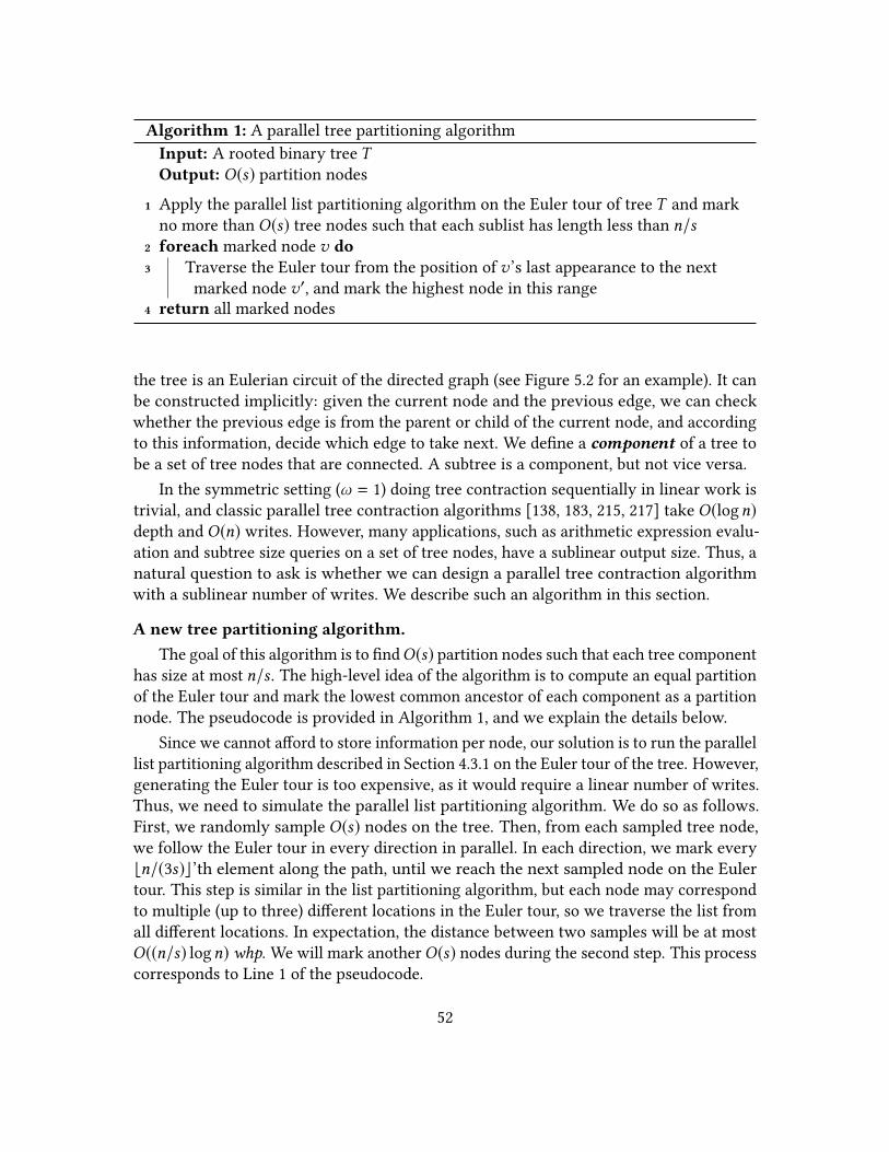
Algorithm 1: A parallel tree partitioning algorithmInput: A rooted binary tree TOutput: O(s) partition nodes

1 Apply the parallel list partitioning algorithm on the Euler tour of tree T and markno more than O(s) tree nodes such that each sublist has length less than n/s

2 foreach marked node v do

3 Traverse the Euler tour from the position of v’s last appearance to the nextmarked node v′, and mark the highest node in this range

4 return all marked nodes

the tree is an Eulerian circuit of the directed graph (see Figure 5.2 for an example). It canbe constructed implicitly: given the current node and the previous edge, we can checkwhether the previous edge is from the parent or child of the current node, and accordingto this information, decide which edge to take next. We dene a component of a tree tobe a set of tree nodes that are connected. A subtree is a component, but not vice versa.

In the symmetric setting (ω = 1) doing tree contraction sequentially in linear work istrivial, and classic parallel tree contraction algorithms [138, 183, 215, 217] take O(logn)depth and O(n) writes. However, many applications, such as arithmetic expression evalu-ation and subtree size queries on a set of tree nodes, have a sublinear output size. Thus, anatural question to ask is whether we can design a parallel tree contraction algorithmwith a sublinear number of writes. We describe such an algorithm in this section.

A new tree partitioning algorithm.

The goal of this algorithm is to ndO(s) partition nodes such that each tree componenthas size at most n/s . The high-level idea of the algorithm is to compute an equal partitionof the Euler tour and mark the lowest common ancestor of each component as a partitionnode. The pseudocode is provided in Algorithm 1, and we explain the details below.

Since we cannot aord to store information per node, our solution is to run the parallellist partitioning algorithm described in Section 4.3.1 on the Euler tour of the tree. However,generating the Euler tour is too expensive, as it would require a linear number of writes.Thus, we need to simulate the parallel list partitioning algorithm. We do so as follows.First, we randomly sample O(s) nodes on the tree. Then, from each sampled tree node,we follow the Euler tour in every direction in parallel. In each direction, we mark everybn/(3s)c’th element along the path, until we reach the next sampled node on the Eulertour. This step is similar in the list partitioning algorithm, but each node may correspondto multiple (up to three) dierent locations in the Euler tour, so we traverse the list fromall dierent locations. In expectation, the distance between two samples will be at mostO((n/s) logn) whp. We will mark anotherO(s) nodes during the second step. This processcorresponds to Line 1 of the pseudocode.

52

Y X

Y

Y

XX

X

Figure 4.2: An example of how the tree is partitioned into components. A component consists oftree nodes from at most three segments of the Euler tour.

With the O(s) marked nodes, the algorithm now nds and marks O(s) partitionnodes, which corresponds to Lines 2–4 of Algorithm 1. A partition node is the highestnode (closest to the root) in a tree component consisting of tree nodes in a segment ofthe Euler tour. For every segment that starts with the rst or second appearance of amarked interior node v , the partition node is just the rst node in the segment, becausethe segment cannot go beyond the subtree of v and it terminates no later than the nextappearance of v in the Euler tour. Hence, we need to do nothing for these segments sincethe partition nodes are already marked. We only consider the segments that start withthe last appearances of marked nodes. The partition node of each such segment can becomputed with constant space by traversing through the segment: we always maintaina pointer p to the highest node so far in the traversal. We start by pointing at the rstnode in the segment, and whenever we go from our current top node to its parent in thetraversal, we update p to point to its parent as well. When the traversal nishes, the nodepointed by p is marked. It is easy to see that this marked node is the highest node in thesegment.

The partition nodes provide a partitioned tree with O(s) components if we form thetree components by ignoring edges from all partition nodes to their parents. We nowshow that this partition is an equal partition.

Lemma 4.3.2. The marked nodes generated in Algorithm 1 partition the tree such that eachtree component contains at most n/s tree nodes.

Proof. We prove this by showing that each component consists of tree nodes from atmost three segments of the Euler tour, which is shown in Figure 4.2. Recall that in the

53

algorithm, we marked every bn/3sc’th element in the Euler tour, so showing this sucesto prove our claim.

In Figure 4.2, nodes marked by the list partitioning algorithm are shown with theletter “X”, and the newly-added partition nodes corresponding to the highest nodes ineach segment are marked with “Y”. Both types of nodes are considered marked nodes. Weclaim that for each tree component rooted by either an X node or a Y node (e.g., the blueregion in Figure 4.2), there exist at most two subtrees (e.g., the two yellow regions inFigure 4.2) that contain marked nodes and are rooted at nodes that are direct children ofthis component. More specically, there will be at most one such subtree in each of theleft and right subtrees of the root node (we will refer to these two subtrees as left-sideand right-side marked subtrees). The segment from the last X node in the left subtree (if itexists) on the Euler tour to the rst X node in the right subtree (if it exists) marks the rootof this component. To see that there is at most one subtree on each side, assume for thesake of contradiction that there are two marked nodes on the same side of the root butnot in the same marked subtree (yellow region). Then the lowest common ancestor ofthese two nodes will be marked as a Y node. This node is assumed to be in this component(the blue region) but actually it will be marked and removed from this component, whichleads to a contradiction.

Hence, each component only consists of nodes from at most three segments fromthe Euler tour. The rst segment is the one that enters this component in the Euler tour,and ends at the rst X node (based on the Euler tour) in the left-side marked subtree,which is shown as the red arrows in Figure 4.2. The second segment is illustrated as theorange arrows, starting from the last X node in the left-side marked subtree and endingin the rst X node in the right-side marked subtree. The last segment, shown as the greenarrows, is symmetric to the rst segment and leaves this part from the last X node. Ifthere are no marked node in the left side, then the rst and second segments are mergedinto one, and similarly on the right side. Thus each component consists of vertices fromat most three segments of the Euler tour.

Since we can guarantee that each segment has size no more than n/3s , each treecomponent contains no more than n/s nodes.

The overall cost is the sum of the cost of partitioning the Euler tour and the cost oftraversing a subset of the segments (starting for the up-edge of each X node). This takeslinear work, O(s) writes and O((n/s) logn) depth whp.

Remark: Notice that our tree partition is done by removing (actually ignoring) edgesbut not vertices (as done in [138]) since this is more ecient on both work and writes inpractice. This algorithm also works on all constant-degree trees. However, for an arbitrarytree our algorithm would not work. In fact, if the given tree is a star, then there doesnot exist any equal partition of non-constant (ω(1)) size, which means that no top-downapproaches by tree partitioning will give a write-ecient solution in this case. Therefore,

54

a preprocessing step that converts the input to a binary tree with linear writes is requiredbefore running our algorithm, but if the tree contraction is run multiple times on a giventree, there is still an advantage in using this algorithm.

A sequential algorithm.

We now discuss a sequential and space-bounded tree contraction algorithm that will beused as a subroutine in our parallel algorithm. Previous tree contraction algorithms [138,215, 217, 254] take either linear space or linear writes to the main memory, which is toocostly in the asymmetric setting. Instead we would like to design an algorithm that uses asmall amount of local (small) memory and performs no writes to main memory. The toolwe use is the tree partitioning algorithm discussed in the previous section, which can beused to partition a tree into components of size no more than n/s using O(s) writes. Ouralgorithm then contracts each tree component down to a single node, and after that weapply a standard tree contraction algorithm on the marked nodes. To restrict the numberof components as well as the size of the components so that all intermediate results tinto a small memory and require no writes, the we recursively apply the tree partitioningalgorithm until each component ts in small memory. Suppose that the cuto size for thebase case of the recursion is c . Then the required small memory size is O(s logs(n/c) + c),and the work and number of reads is O(n logs(n/c)). By setting s to either O(ϵnϵ ) or someconstant greater than 1, we obtain the following lemma.

Lemma 4.3.3. The sequential algorithm presented above contracts a tree of size n requiringO(1) writes, and using a small memory of size O(nϵ ) and linear work, where 0 < ϵ < 1, or asmall memory of size O(logn) and O(n logn) work and reads.

A parallel algorithm.

We now describe a parallel tree-contraction algorithm that uses the tree partitioningalgorithm and sequential tree contraction algorithm as subroutines.

The high-level idea for the parallel algorithm is to rst partition the tree into small,almost equal-sized components using the tree partitioning algorithm, and then contracteach component independently in parallel using the sequential contraction algorithm.Finally, we use a standard parallel tree contraction algorithm to contract the remainingnodes. This step requires a number of writes proportional to the number of remainingnodes, which is much smaller than the original tree size. The algorithm takes s as aparameter and consists of three steps as described below.

Step 1: Tree Partitioning. The rst part of the algorithm computes a tree partitionsuch that each component has size O(n/s), where s is a parameter of the algorithm. Thisstep requires O(n) work, O((n logn)/s) depth whp and O(s) writes, if implemented byAlgorithm 1.

Step 2: Tree Contraction on Components. With the partition nodes computed inStep 1, we now have a set of components each with size at most O(n/s). Since the

55

tree components are themselves trees, we can apply our sequential tree contractionalgorithm on each of them. The contraction is restricted to be inside each componentby not contracting any partition node. Also, we leave the root node of each componentuncontracted. After contraction, each component’s root has at most one left and one rightchild, which is either the marked child (the Y nodes in the yellow regions in Figure 4.2)or the a descendant of the root that is in the component (if no marked child on the side).Hence, if the local memory has sizeO((n/s)ϵ ), this step takes linear time andO(n/s) depth,and yields an intermediate contracted tree with no more than O(s) nodes.

Step 3: Contraction of Remaining Nodes. In the last step, we apply any existingparallel tree contraction algorithm with linear work and logarithmic depth to contractthe tree generated from the last step to a single node. This step costs O(s) reads, writesand work, and O(logn) depth.

To reduce the number of writes without increasing the asymptotic work complexity,we choose s = n/ω. Hence, the size of the components is at most ω. The followingtheorem gives the cost of our parallel tree contraction algorithm.Theorem 4.3.4. Algorithm 1 can be used to contract a tree with size n using O(n) work,O(ω logn) depth and O(n/ω) writes with O(ωϵ ) local memory in the Asymmetric NP model.

4.4 Sorting

For sorting algorithm, we rst observe that in the RAM model, it is well known thatsorting by inserting each key into a balanced search tree requires only O(n) writes withno increase in reads (O(n logn)). However, applying the idea to the Asymmetric NP modelis non-trivial, since the well-known parallel sorting algorithms with O(logn) depth, likeCole’s mergesort [102], do not t into the two framework we discussed in Section 2.3.2.Instead, we extend the parallel sorting algorithm in [68] into a write-ecient manner, andyield an algorithm with O(n) writes, O(n logn) reads and O(logn) depth whp assumingpriority writes (Section 4.4.2).

Since sorting is one of the most fundamental algorithm and widely used as a subroutinein many other algorithms and frameworks, we also consider it on the (M,B,ω)-ARAM(considering the block size B). We show that three asymptotically-optimal sorting al-gorithms can each be adapted to the (M,B,ω)-ARAM with reduced write costs. First,following [226, 273], we adapt multi-way mergesort by merging ωM/B sorted runs at atime (instead of M/B as in the original EM version). This change saves writes by reducingthe depth of the recursion. Each merge makesω passes over the runs, using an in-memoryheap to extract values for the output run for the pass. Our algorithm and analysis issomewhat simpler than [226, 273]. Second, we present a sample sort algorithm that usesωM/B splitters at each level of recursion (instead of M/B in the original EM version).Again, the challenge is to both nd the splitters and partition using them while incurringonlyO(N /B) writes across each level of recursion. Finally, our third sorting algorithm is a

56

Algorithm 2: Asymmetric-NP SortInput: An array of records A of length nOutput: The sorted array

1 Select a sample S from A independently at random with per-record probability1/logn, and sort the sample

2 Use every (logn)-th element in the sorted S as splitters, and for each of the aboutn/log2 n buckets dened by the splitters allocate an array of size c log2 n

3 In parallel locate each record’s bucket using a binary search on the splitters4 In parallel insert the records into their buckets by repeatedly trying a random

position within the associated array and attempting to insert if empty5 Pack out all empty cells in the arrays and concatenate all arrays// Step 6 is an optional step used to obtain O(ω logn) depth

6 for round r ← 1 to 2 do

7 foreach array A′ generated in previous round (in parallel) do8 Deterministically select |A′|1/3 − 1 samples as splitters and apply integer

sort on the bucket number to partition A′ into |A′|1/3 sub-arrays9 foreach subarray from the previous round do

10 Apply the (M,ω)-ARAM sort11 return the sorted array

heapsort using a buer-tree-based priority queue. Compared to the original EM algorithm,both our buer-tree nodes and the number of elements stored outside the buer tree arelarger by a factor of ω, which adds nontrivial changes to the data structure. All threesorting algorithms have the same asymptotic complexity on the (M,B,ω)-ARAM.

4.4.1 Sorting on (M,ω)-ARAM

The number of writes on an (M,ω)-ARAM can be bound for a variety of algorithms anddata structures using known techniques. For example, based on the analysis of balancedbinary search trees in the previous sections, many trees only require a constant numberof rotations per insertion and deletion. Sorting can be done by inserting n records intoa balanced search tree data structure, and then reading them o in order. This requiresO(n logn) reads andO(n) writes, for total costO(n(ω + logn)). Similarly, we can maintainpriority queues (insert and delete-min) and comparison-based dictionaries (insert, deleteand search) in O(1) writes per operation.

4.4.2 Sorting on Asymmetric NP Model

We now consider how to sort on the Asymmetric NP model allowing arbitrary write.Algorithm 2 outlines a sample sort (with over-sampling) that does O(n logn + ωn) work

57

(O(n logn) reads and O(n) writes) and has depth O(log2 n

). It is similar to other sample

sorts [56, 127, 183]. We consider each step in more detail and analyze its cost.Step 1 can use Cole’s parallel mergesort [102] requiring O(n) reads and writes whp

(because the sample is size Θ(n/logn) whp), andO(ω logn) depth. In step 2 for sucientlylarge c , whp all arrays will have at least twice as many slots as there are records belongingto the associated bucket [56]. The cost of step 2 is a lower-order term. Step 3 requiresO(n logn) reads, O(n) writes and O(logn) depth for the binary searches and writing theresulting bucket numbers. Step 4 is an instance of the so-called placement problem(see [236, 239]). This can be implementing by having each record select a random locationwithin the array associated with its bucket and if empty, attempting to insert the recordat that location. This is repeated if unsuccessful. Since multiple records might try thesame location at the same time, each record needs to check if it was successfully inserted.The expected number of tries per record is constant. Also, if the records are partitionedinto groups of size logn and processed sequentially within the group and in parallelacross groups, then whp no group will require more than O(logn) tries across all of itsrecords [236]. Therefore, whp the number of reads and writes for this step are O(n) andthe depth is O(logn). Step 5 can be done with a prex sum, requiring a linear numberof reads and writes, and O(logn) depth. At this point we could apply the asymmetricRAM sort to each bucket giving a total of O(n logn) reads, O(n) writes and a depth ofO

(log2 n log logn

)whp.

We can reduce the depth to O(logn) by further deterministically sampling inside eachbucket (step 6) using the following lemma:

Lemma 4.4.1. We can partitionm records intom1/3 buckets M1, . . . ,Mm1/3 such that forany i and j where i < j all records in Mi are less than all records in Mj , and for all i ,|Mi | < m

2/3 logm. The process requires O(m logm) reads, O(m) writes, and O(ω√m

)depth.

Proof. We rst split them records into groups of sizem1/3 and sort each group with theRAM sort. This takes O(m logm) reads, O(m) writes and O

(m1/3 logm

)depth. Then for

each sorted group, we place every logm’th record into a sample. Now we sort the sampleof size m/logm using Cole’s mergesort, and use the result as splitters to partition theremaining records into buckets. Finally, we place the records into their respective bucketsby integer sorting the records based on their bucket number. This can be done with aparallel radix sort in a linear number of reads/writes and O

(√m

)depth [236].

To show that the largest bucket has size at mostm2/3 logm, note that in each bucket, wecan pick at most logm consecutive records from each of the m2/3 groups without pickinga splitter. Otherwise there will be a splitter in the bucket, which is a contradiction.

Step 6 applies two iterations of Lemma 4.4.1 to each bucket to partition it into sub-buckets. For an initial bucket of size m, this process will create sub-buckets of at mostsizeO

(m4/9 log5/3m

). Plugging inm = O

(log2 n

)gives us that the largest sub-bucket is of

58

size O(log8/9 n(log logn)5/3

). We can now apply the RAM sort to each bucket in O(logn)

depth. This gives us the following theorem.

Theorem 4.4.2. Sorting n records can be performed usingO(n logn +ωn) work (O(n logn)reads and O(n) writes), and in O

(log2 n

)depth whp on the Asymmetric NP model allowing

concurrent writes.

Reducing the depth toO(logn). The depth can be reduced toO(logn) by combining theresult of the sorting algorithm by Jeremy Fineman, which can sort n elements inO(n logn)reads and writes and O(logn) depth on the nested-parallel model. The algorithm isrecursive. In each level, we assume the problem size is m. We pick s =

√m/logn samples,

using a O(s2) algorithm to sort them in O(log s) time, and then subselect p = s/logn aspivots. Then by using the solution for placement problems to put every element intothe correct bucket. This algorithm stops when there is less than O(log6 n) elements ineach bucket. Then elements within each bucket can be sorted using any polylog-depthalgorithm. This algorithm is not write-ecient, but can be used to replace Cole’s mergesortin Step 1 to achieve O(logn) depth whp.

4.4.3 Sorting on (M,B,ω)-ARAMModel

In this section, we present sorting algorithms for the (M,B,ω)-ARAM model. Weshow how the three approaches for external-memory sorting—mergesort, sample sort,and heapsort (using buer trees)—can each be adapted to this asymmetric case.

In each case we trade o a factor of ω additional reads for a larger branching factor(ωM/B instead of M/B), hence reducing the number of rounds. The ARAM cost of eachalgorithm matches the non-trivial lower bound given in Section 3.5. It is interesting thatthe same general approach works for all three types of sorting. The rst algorithm, themergesort, has been described elsewhere [226] although in a dierent model (their modelis specic to NAND ash memory and has dierent sized blocks for reading and writing,among other dierences). Our parameters are therefore dierent, and our analysis is new.//about Nodari. To the best of our knowledge, our other two algorithms are new.

4.4.3.1 Mergesort

We use an l-way mergesort—i.e., a balanced tree of merges with each merge taking inl sorted arrays and outputting one sorted array consisting of all records from the input.We assume that once the input is small enough a dierent sort (the base case) is applied.For l = M/B and a base case of n ≤ M (using any sort since it ts in memory), we havethe standard EM mergesort. With these settings there are logM/B(n/M) levels of recursion,plus the base case, each costing O(n/B) memory operations. This gives the well-knownoverall bound of Θ((n/B) logM/B(n/B)) [7].

To modify the algorithm for the asymmetric case, we increase the branching factor andthe base case by a factor ofω, i.e., l = ωM/B and a base case of n ≤ ωM . This means that it

59

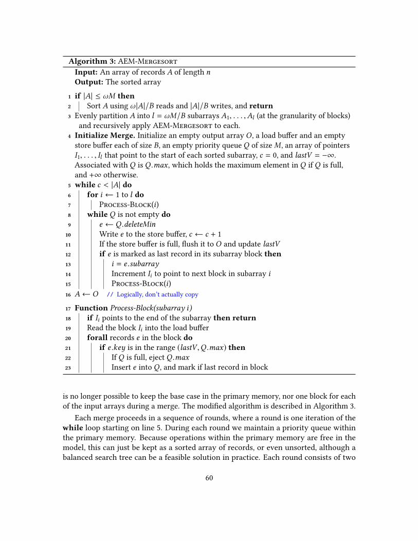
Algorithm 3: AEM-MergesortInput: An array of records A of length nOutput: The sorted array

1 if |A| ≤ ωM then

2 Sort A using ω |A|/B reads and |A|/B writes, and return

3 Evenly partition A into l = ωM/B subarrays A1, . . . ,Al (at the granularity of blocks)and recursively apply AEM-Mergesort to each.

4 Initialize Merge. Initialize an empty output array O , a load buer and an emptystore buer each of size B, an empty priority queue Q of size M , an array of pointersI1, . . . , Il that point to the start of each sorted subarray, c = 0, and lastV = −∞.Associated with Q is Q .max, which holds the maximum element in Q if Q is full,and +∞ otherwise.

5 while c < |A| do6 for i ← 1 to l do7 Process-Block(i)8 while Q is not empty do

9 e ← Q .deleteMin10 Write e to the store buer, c ← c + 111 If the store buer is full, ush it to O and update lastV12 if e is marked as last record in its subarray block then

13 i = e .subarray14 Increment Ii to point to next block in subarray i15 Process-Block(i)16 A← O // Logically, don’t actually copy

17 Function Process-Block(subarray i)18 if Ii points to the end of the subarray then return

19 Read the block Ii into the load buer20 forall records e in the block do

21 if e .key is in the range (lastV ,Q .max) then22 If Q is full, eject Q .max23 Insert e into Q , and mark if last record in block

is no longer possible to keep the base case in the primary memory, nor one block for eachof the input arrays during a merge. The modied algorithm is described in Algorithm 3.

Each merge proceeds in a sequence of rounds, where a round is one iteration of thewhile loop starting on line 5. During each round we maintain a priority queue withinthe primary memory. Because operations within the primary memory are free in themodel, this can just be kept as a sorted array of records, or even unsorted, although abalanced search tree can be a feasible solution in practice. Each round consists of two

60

phases. The rst phase (the for loop on line 6) considers each of the l input subarrays inturn, loading the current block for the subarray into the load buer, and then insertingeach record e from the block into the priority queue if not already written to the output(i.e., e .key > lastV ), and if smaller than the maximum in the queue (i.e., e .key < Q .max).This might bump an existing element out of the queue. Also, if a record is the last in itsblock then it is marked and tagged with its subarray number.

The second phase (the while loop starting on line 8) starts writing the priority queueto the output one block at a time. Whenever reaching a record that is marked as thelast in its block, the algorithm increments the pointer to the corresponding subarray andprocesses the next block in the subarray. We repeat the rounds until all records from allsubarrays have been processed.

To account for the space for the pointers I = I1, . . . , Il , let α = (logn)/s , where s is thesize of a record in bits, and n is the total number of records being merged. The cost of themerge is bounded as follows:

Lemma 4.4.3. l = ωM/B sorted sequences with total size n (stored in dn/Be blocks, andblock aligned) can be merged using at most (ω + 1)dn/Be reads and dn/Be writes, on the(M,B,ω)-ARAM model with primary memory size (M + 2B + 2αωM/B).

Proof. Each round (except perhaps the last) outputs at least M records, and hence the totalnumber of rounds is at most dn/Me. The rst phase of each round requires at most ωM/Breads, so the total number of reads across all the rst phases is at most ω dn/Be (the lastround can be included in this since it only loads as many blocks as are output). For thesecond phase, a block is only read when incrementing its pointer, therefore every block isonly read once in the second phase. Also every record is only written once. This gives thestated bounds on the number of reads and writes. The space includes the space for thein-memory heap (M), the load and store buers, the pointers I (αωM/B), and pointers tomaintain the last-record in block information (αωM/B).

We note that it is also possible to keep I in secondary memory. This will double thenumber of writes because every time the algorithm moves to a new block in an inputarray i , it would need to write out the updated Ii . The increase in reads is small. Also, ifone uses a balanced search tree to implement the priority queue Q then the size increasesby < M(logM)/s in order to store the pointers in the tree.

For the base case when n ≤ ωM we use the following lemma.

Lemma 4.4.4. n ≤ ωM records stored in dn/Be blocks can be sorted using at most ω dn/Bereads and dn/Be writes, on the (M,B,ω)-ARAM model with primary memory sizeM + B.

Proof. We sort the elements using a variant of selection sort, scanning the input list atotal of at most ω times. In the rst scan, store in memory the M smallest elements seenso far, performing no writes and dn/Be reads. After completing the scan, output all themin(M,n) elements in sorted order using dmin(M,n)/Be writes. Record the maximum

61

element written so far. In each subsequent phase (if not nished), store in memory the Msmallest records larger than the maximum written so far, then output as before. The costis dn/Be reads and M/B writes per phase (except perhaps the last phase). We need oneextra block to hold the input. The largest output can be stored in the O(logM) locationswe have allowed for in the model. This gives the stated bounds because every element iswritten out once and the input is scanned at most ω times.

Together we have:

Theorem 4.4.5. Algorithm 3 sorts n records using

R(n) ≤ (ω + 1)⌈nB

⌉⌈logωM

B

(nB

)⌉reads, and

W (n) ≤⌈nB

⌉⌈logωM

B

(nB

)⌉writes on an (M,B,ω)-ARAM with primary memory size (M + 2B + 2αωM/B).

Proof. The number of recursive levels of merging is bounded by⌈logωM

B

( nωM

)⌉, and when

we add the additional base round we have 1 +⌈logωM

B

( nωM

)⌉=

⌈logωM

B

( nωM

ωMB

)⌉=⌈

logωMB

( nB

)⌉. The cost for each level is at most (ω + 1)dn/Be reads and dn/Be writes

(only one block on each level might not be full).

4.4.3.2 Sample Sort

We now describe an l-way randomized sample sort [56, 127] (also called distributionsort), which asymptotically matches the I/O bounds of the mergesort. The idea of samplesort is to partition n records into l approximately equally sized buckets based on a sampleof the keys within the records, and then recurse on each bucket until an appropriately-sized base case is reached. As with the mergesort, here we will use a branching factorl = ωM/B. Again this branching factor will reduce the number of levels of recursionrelative to the standard EM sample sort which uses l = M/B [7]. We describe how toprocess each partition and the base case.

The partitioning starts by selecting a set of splitters. This can be done using standardtechniques, which we review later. The splitters partition the input into buckets that whpare within a constant factor of the average size n/l . The algorithm now needs to bucketthe input based on the splitters. The algorithm processes the splitters in ω rounds of sizeM/B each, starting with the rst M/B splitters. For each round the algorithm scans thewhole input array, partitioning each value into the one of M/B buckets associated withthe splitters, or skipping a record if its key does not belong in the current buckets. Oneblock for each bucket is kept in memory. Whenever a block for one of the buckets is full,it is written out to memory and the next block is started for that bucket. Each ω rounds

62

reads all of the input and writes out only the elements associated with these buckets(roughly a 1/ω fraction of the input).

The base case occurs when n ≤ ωM , at which point we apply the selection sort fromLemma 4.4.4.

Let n0 be the original input size. The splitters can be chosen by randomly pickinga sample of keys of size m = Θ(l logn0), sorting them, and then sub-selecting the keysat positions m/l, 2m/l, . . . , (l − 1)m/l . By selecting the constant in the Θ sucientlylarge, this process ensures that, whp every bucket is within a constant factor of theaverage size [56]. To sort the samples apply a RAM mergesort, which requires at mostO(((l logn0)/B) log(l logn0/M)) reads and writes. This is a lower-order term when l =O(n /log2 n), but unfortunately this bound on l may not hold for small subproblems. Thereis a simple solution—when n ≤ ω2M2/B, instead use l = n/(ωM). With this modication,we always have l ≤

√n/B.

It is likely that the splitters could also be selected deterministically using an approachused in the original I/O-ecient distribution sort [7].Theorem 4.4.6. The kM/B-way sample sort sorts n records using, whp,

R(n) = O(ωnB

⌈logωM

B

(nB

)⌉)reads, and

W (n) = O(nB

⌈logωM

B

(nB

)⌉)writes on an (M,B,ω)-ARAM with primary memory size (M + B +M/B).

Proof. (Sketch) The primary-memory size allows one block from each bucket as well as theM/B splitters to remain in memory. Each partitioning step thus requires dn/Be + ωM/Bwrites, where the second term arises from the fact that each bucket may use a partial block.Since n ≥ ωM (this is not a base case), the cost of each partitioning step becomes O(n/B)writes and O(kn/B) reads. Because the number of splitters is at most

√n = O(n/log2 n),

choosing and sorting the splitters takesO(n/B) reads and writes. Observe that the recursivestructure matches that of a sample sort with an eective memory of size ωM , and thatthere will be at most two rounds at the end where l = n/(ωM). As in standard samplesort, the number of writes is linear with the size of the subproblem, but here the numberof reads is multiplied by a factor of ω. The standard samplesort analysis thus applies,implying the bound stated.

It remains only to consider the base case. Because all buckets are approximately thesame size, the total number of leaves is O(n/B)—during the recursion, a size n > ωMproblem is split into subproblems whose sizes are Ω(B). Applying Lemma 4.4.4 to allleaves, we get a cost of O(ωn/B) reads and O(n/B) writes for all base cases.

Extensions for the Private-Cache Model. The above can be readily parallelized. Herewe outline the approach. We assume that there arep = n/M processors. We use parallelism

63

both within each partition, and across the recursive partitions. Within a partition we rstnd the l splitters in parallel. (As above, l = ωM/B except for the at most two rounds priorto the base case where l = n/(ωM).) This can be done on a sample that is a logarithmicfactor smaller than the partition size, using a less ecient sorting algorithm such asparallel mergesort, and then sub-selecting l splitters from the sorted order. This requiresO(ω(M/B + log2 n)) time, where the second term (O(ω log2 n)) is the depth of the parallelmergesort, and the rst term is the work term O((ω/B)((n/logn) logn)/P) = O(ωM/B).

The algorithm groups the input into n/(ωM) chunks of size ωM each. As before wealso group the splitters into ω rounds of size M/B each. Now in parallel across all chunksand across all rounds, partition the chunk based on the round. We have n/(ωM)×ω = n/Mprocessors so we can do them all in parallel. Each will require ωM reads and M writes.To ensure that the chunks write their buckets to adjacent locations (so that the output ofeach bucket is contiguous) we will need to do a pass over the input to count the size ofeach bucket for each chunk, followed by a prex sum. This can be done before processingthe chunks and is a lower-order term. The time for the computation is O(ωM/B).

The processors are then divided among the sub-problems proportional to the size ofthe sub-problem, and we repeat. The work at each level of recursion remains the same, sothe time at each level remains the same. For the base case of size ≤ ωM , instead of using aselection sort across all keys, which is sequential, we nd ω splitters and divide the workamong ω processors to sub-select their part of the input, each by reading the whole input,and then sorting their part of size O(M) using a selection sort on those keys. This againtakes O(ωM/B) time. The total time for the algorithm is therefore:

O

(ω

(M

B+ log2 n

)⌈1 + logωM

B

( n

ωM

)⌉)with high probability. This is linear speedup assuming M

B ≥ log2 n. Otherwise the numberof processors can be reduced to maintain linear speedup.

4.4.3.3 I/O Buer Trees

This section describes how to augment the basic buer tree [25] to build a priorityqueue that supports n Insert and Delete-Min operations with an amortized cost ofO((ω/B)(1 + logωM/B n)) reads and O((1/B)(1 + logωM/B n)) writes per operation. Usingthe priority queue to implement a sorting algorithm trivially results in a sort costing atotal ofO((ωn/B)(1+ logωM/B n)) reads andO((n/B)(1+ logωM/B n)) writes. These boundsasymptotically match the preceding sorting algorithms, but some additional constantfactors are introduced because a buer tree is a dynamic data structure.

Our buer tree-based priority queue for the (M,B,ω)-ARAM contains a few dierencesfrom the regular EM buer tree [25]: (1) the buer tree nodes are larger by a factor ω,(2) consequently, the “buer-emptying” process uses an ecient sort on ωM elementsinstead of an in-memory sort on M elements, and (3) to support the priority queue,O(ωM)

64

elements are stored outside the buer tree instead ofO(M), which adds nontrivial changesto the data structure.

Overview of a buer tree.

A buer tree [25] is an augmented version of an (a,b)-tree [175], where a = l/4 andb = l for large branching factor l . In the original buer tree l = M/B, but to reduce thenumber of writes we instead set l = ωM/B. As an (a,b) tree, all leaves are at the samedepth in the tree, and all internal nodes have between l/4 and l children (except the root,which may have fewer). Thus the height of the tree is O(1 + logl n). An internal nodewith c children contains c − 1 keys, stored in sorted order, that partition the elementsin the subtrees. The structure of a buer tree diers from that of an (a,b) tree in twoways. Firstly, each leaf of the buer tree contains between lB/4 and lB elements stored inl blocks.1 Secondly, each node in the buer tree also contains a dense unsorted list, calleda buer, of partially inserted elements that belong in that subtree.

We next summarize the basic buer tree insertion process [25]. Supporting generaldeletions is not much harder, but to implement a priority queue we only need to supportdeleting an entire leaf. The insertion algorithm proceeds in two phases: the rst phasemoves elements down the tree through buers, and the second phase performs the (a,b)-tree rebalance operations (i.e., splitting nodes that are too big). The rst phase begins byappending the new element to the end of the root’s buer. We say that a node is full ifits buer contains at least lB elements. If the insert causes the root to become full, then abuer-emptying process commences, whereby all of the elements in the node’s buerare sorted then distributed to the children (appended to the ends of their buers). Thisdistribution process may cause children to become full, in which case they must also beemptied. More precisely, the algorithm maintains a list of internal nodes with full buers(initially the root) and a separate list of leaves with full buers. The rst phase operatesby repeatedly extracting a full internal node from the list, emptying its buer, and addingany full children to the list of full internal or leaf nodes, until there are no full internalnodes.

Note that during the rst phase, the buers of full nodes may far exceed lB, e.g., if allof the ancestors’ buer elements are distributed to a single descendant. Sorting the buerfrom scratch would therefore be too expensive. Fortunately, each distribution processwrites elements to the child buers in sorted order, so all elements after the lB’th element(i.e., those written in the most recent emptying of the parent) are sorted. It thus sucesto split the buer at the lB’th element and sort the rst lB elements, resulting in a buerthat consists of two sorted lists. These two lists can trivially be merged as they are beingdistributed to the sorted list of children in a linear number of I/O’s.

1Arge [25] denes the “leaves” of a buer tree to contain Θ(B) elements instead of Θ(lB) elements. Sincethe algorithm only operates on the parents of those “leaves”, we nd the terminology more convenient whenattening the bottom two levels of the tree. Our leaves thus correspond to what Arge terms “leaf nodes” [25](not to be confused with leaves) or equivalently what Sitchinava and Zeh call “fringe nodes” [256].

65

When the rst phase completes, there may be full leaves but no full internal nodes.Moreover, all ancestors of each full leaf have empty buers. The second phase operateson each full leaf one at a time. First, the buer is sorted as above and then merged withthe elements stored in the leaf. If the leaf contains X > lB elements, then a sequence of(a,b)-tree rebalance operations occur whereby the leaf may be split into Θ(X/(lB)) newnodes. These splits cascade up the tree as in a typical (a,b)-tree insert.

Buer tree with fewer writes.

To reduce the number of writes, we set the branching factor of the buer tree tol = ωM/B instead of l = M/B. The consequence of this increase is that the bueremptying process needs to sort lB = ωM elements, which cannot be done with an in-memory sort. The advantage is that the height of the tree reduces to O(1 + logωM/B n).

Lemma 4.4.7. It costs O(ωX/B) reads and O(X/B) writes to empty a full buer containingX elements using Θ(M) memory.

Proof. By Lemma 4.4.4, the cost of sorting the rst ωM elements is O(ω2M/B) reads andO(ωM/B) writes. The distribute step can be performed by simultaneously scanning thesorted list of children along with the two sorted pieces of the buer, and outputting to theend of the appropriate child buer. A write occurs only when either nishing with a childor closing out a block. The distribute step thus uses O(ωM/B + X/B) reads and writes,giving a total of O(ω2M/B + X/B) reads and O(ωM/B + X/B) writes including the sortstep. Observing that full means X > ωM completes the proof.

Theorem 4.4.8. Suppose that the partially empty block belonging to the root’s buer iskept in memory. Then the amortized cost of each insert into an n-element buer tree isO((ω/B)(1 + logωM/B n)) reads and O((1/B)(1 + logωM/B n)) writes.

Proof. This proof follows from Arge’s buer tree performance proofs [25], augmentedwith the above lemma. We rst consider the cost of reading and writing the buers. Thelast block of the root buer need only be written when it becomes full, at which point thenext block must be read, giving O(1/B) reads and writes per insert. Each element movesthrough buers on a root-to-leaf path, so it may belong to O(1 + logωM/B n) emptyingprocesses. According to Lemma 4.4.7, emptying a full buer costs O(ω/B) reads andO(1/B) writes per element. Multiplying these two gives an amortized cost per elementmatching the theorem.

We next consider the cost of rebalancing operations. Given the choice of (a,b)-tree pa-rameters, the total number of node splits isO(n/(lB)) [25, Theorem 1] which isO(n/(ωM)).Each split is performed by scanning a constant number of nodes, yielding a cost ofO(ωM/B) reads and write per split, or O(n/(ωM) · ωM/B) = O(n/B) reads and writes intotal or O(1/B) per insert.

An ecient priority queue with fewer writes.

66

The main idea of Arge’s buer tree-based priority queue [25] is to store a workingset of the O(lB) smallest elements resident in memory. When inserting an element, rstadd it to the working set, then evict the largest element from the working set (perhapsthe one just inserted) and insert it into the buer tree. To extract the minimum, nd it inthe working set. If the working set is empty, remove the Θ(lB) smallest elements fromthe buer tree and add them to the working set. In the standard buer tree, l = M/B andhence operating on the working set is free because it ts entirely in memory. In our case,however, extra care is necessary to maintain a working set that has size roughly ω timeslarger.

Our (M,B,ω)-ARAM priority queue follows the same idea except the working setis partitioned into two pieces, the alpha working set and beta working set. The alphaworking set, which is always resident in memory, contains at most M/4 of the smallestelements in the priority queue. The beta working set contains at most 2ωM of the nextsmallest elements in the data structure, stored in O(ωM/B) blocks. The motivation forhaving a beta working set is that during Delete-Min operations, emptying elementsdirectly from the buer tree whenever the alpha working set is empty would be tooexpensive—having a beta working set to stage larger batches of such elements leads tobetter amortized bounds. Coping with the interaction between the alpha working set, thebeta working set, and the buer tree, is the main complexity of our priority queue. Thebeta working set does not t in memory, but we keep a constant number of blocks fromthe beta working set and the buer tree (specically, the last block of the root buer) inmemory.

We begin with a high-level description of the priority-queue operations, with detailsof the beta working set deferred until later. For now, it suces to know that we keepthe maximum key in the beta working set in memory. To insert a new element, rstcompare its key against the maximums in the alpha and beta working set. Then insertit into either the alpha working set, the beta working set, or the buer tree dependingon the key comparisons. If the alpha working set exceeds maximum capacity of M/4elements, move the largest element to the beta working set. If the beta working set hitsits maximum capacity of 2ωM elements, remove the largest ωM elements and insert theminto the buer tree.

To delete the minimum from the priority queue, remove the smallest element from thealpha working set. If the alpha working set is empty, extract the M/4 smallest elementsfrom the beta working set (details to follow) and move them to the alpha working set. If thebeta working set is empty, perform a buer emptying process on the root-to-leftmost-leafpath in the buer tree. Then delete the leftmost leaf and move its contents to the betaworking set.

The beta working set. The main challenge is in implementing the beta working set.An unsorted list or buer allows for ecient inserts by appending to the last block. Thechallenge, however, is to extract the Θ(M) smallest elements with O(M/B) writes—if

67

ω > B, each element may reside in a separate block, and we thus cannot aord to updatethose blocks when extracting the elements. Instead, we perform the deletions implicitly.

To facilitate implicit deletions, we maintain a list of ordered pairs (i1, x1), (i2, x2), (i3, x3), . . .,where (i, x) indicates that all elements with index at most i and key at most x are in-valid. Our algorithm maintains the invariant that for consecutive list elements (ij, xj) and(ij+1, xj+1), we have ij < ij+1 and xj > xj+1 (recall that all keys are distinct).

To insert an element to the beta working set, simply append it to the end. The invariantis maintained because its index is larger than any pair in the list.

To extract the minimum M/4 elements, scan from index 0 to i1 in the beta workingset, ignoring any elements with key at most x1. Then scan from i1 + 1 to i2, ignoring anyelement with key at most x2. And so on. While scanning, record in memory the M/4smallest valid elements seen so far. When nished, let x be the largest key and let i bethe length of the beta working set. All elements with key at most x have been removedfrom the full beta working set, so they should be implicitly marked as invalid. To restorethe invariant, truncate the list until the last pair (ij, xj) has xj > x , then append (i, x) tothe list. Because the size of the beta working set is growing, ij < i . It should be clear thattruncation does not discard any information as (i, x) subsumes any of the truncated pairs.

Whenever the beta working set grows too large (2ωM valid elements) or becomes toosparse (ω extractions of M/4 elements each have occurred), we rst rebuild it. Rebuildingscans the elements in order, removing the invalid elements by packing the valid onesdensely into blocks. Testing for validity is done as above. When done, the list of orderedpairs to test invalidity is cleared.

Finally, when the beta working set grows too large, we extract the largestωM elementsby sorting it (using the selection sort of Lemma 4.4.4).

Analyzing the priority queue.

We begin with some lemmas about the beta working set.Lemma 4.4.9. Extracting theM/4 smallest valid elements from the beta working set andstoring them in memory costs O(ωM/B) reads and amortized O(1) writes.

Proof. The extraction involves rst performing read-only passes over the beta workingset and list of pairs, keeping one block from the working set and one pair in memoryat a time. Because the working set is rebuilt after ω extractions, the list of pairs canhave at most ω entries. Even if the list is not I/O ecient, the cost of scanning both isO(ωM/B + ω) = O(ωM/B) reads. Next the list of pairs indicating invalid elements isupdated. Appending one new entry requires O(1) writes. Truncating and deleting any oldentries can be charged against their insertions.

The proof of the following lemma is similar to the preceding one, with the onlydierence being that the valid elements must be moved and written as they are read.Lemma 4.4.10. Rebuilding the beta working set costs O(ωM/B) reads and writes.

68

Theorem 4.4.11. Our priority queue, if initially empty, supports n Insert and Delete-Min operations with an amortized cost of O((ω/B)(1 + logωM/B n)) reads and O((1/B)(1 +logωM/B n)) writes per operation.

Proof. Inserts are the easier case. Inserting into the alpha working set is free. Theamortized cost of inserting directly into the beta working set (a simple append) is O(1/B)reads and writes, assuming the last block stays in memory. The cost of inserting directlyinto the buer tree matches the theorem. Occasionally, the beta working set overows, inwhich case we rebuild it, sort it, and insert elements into the buer tree. The rebuild costsO(ωM/B) reads and writes (Lemma 4.4.10), the sort costs O(ω2M/B) reads and O(ωM/B)writes (by Lemma 4.4.4), and the ωM buer tree inserts cost O((ω2M/B)(1 + logωM/B n))reads and O((ωM/B)(1 + logωM/B n)) writes (by Theorem 4.4.8). The latter dominates.Amortizing against the ωM inserts that occur between overows, the amortized cost perinsert matches the theorem statement.

Deleting the minimum element from the alpha working set is free. When the alphaworking set becomes empty, we extract M/4 elements from the beta working set, with acost ofO(ωM/B) reads andO(1)writes (Lemma 4.4.9). This cost may be amortized againstthe M/4 deletes that occur between extractions, for an amortized cost ofO(ω/B) reads andO(1/M) writes per delete-min. Every ω extractions of M/4 elements, the beta working setis rebuilt, with a cost of O(ωM/B) reads and writes (Lemma 4.4.10) or amortized O(1/B)reads and writes per delete-min. Adding these together, we so far have O(ω/B) reads andO(1/B) writes per delete-min.

It remains to analyze the cost of relling the beta working set when it becomes empty.The cost of removing a leaf from the buer tree is dominated by the cost of emptyingbuers on a length-O(logωM/B n) path. Note that the buers are not full, so we cannotapply Lemma 4.4.7. But a similar analysis applies. The cost per node is O(ω2M/B + X/B)reads and O(ωM/B + X/B) writes for an X -element buer. As with Arge’s version ofthe priority queue [25], the O(X/B) terms can be charged to the insertion of the Xelements, so we are left with a cost of O(ω2M/B) read and O(ωM/B) writes per buer.Multiplying by O(1 + logωM/B n) levels gives a cost of O((ω2M/B)(1 + logωM/B n)) readsand O((ωM/B)(1+ logωM/B n)) writes. Because each leaf contains at least ωM/4 elements,we can amortize this cost against at least ωM/4 deletions, giving a cost that matches thetheorem.

With this priority queue, sorting can be trivially implemented in O((ωn/B)(1 +logωM/B n)) reads andO((n/B)(1+ logωM/B n))writes, matching the bounds of the previoussorting algorithms.

69

4.5 Longest Common Subsequence and Edit Distance

This section describes a more ecient dynamic-programming algorithm for longestcommon subsequence (LCS) and edit distance (ED) on the (M,ω)-ARAM model. Thestandard approach for these problems (an M × M tiling) results in an ARAM cost ofO(mnω/M) and work of O(mn +mnω/M), wherem and n are the length of the two inputstrings. Lemma 3.4.2 states that the standard bound is optimal under the standard DAGcomputation rule that all inputs must be available before evaluating a node. Perhapssurprisingly, we are able to beat these bounds by leveraging the fact that dynamic programsdo not perform arbitrary functions at each node, and hence we do not necessarily needall inputs to begin evaluating a node.

Our main result is captured by the following theorem for large input strings (thegeneral case). For smaller strings, we can do even better and will be discussed later inSection 4.5.2.

4.5.1 The General Case

Theorem 4.5.1. Let kT = min((ω/M)1/3,√M) and suppose m,n = Ω(kTM). Then it is

possible to compute the ED or length of the LCS with workW (m,n) = O(mn +mnω/(kTM)).Let kQ = min(ω1/3,

√M) and supposem,n = Ω(kQM). Then it is possible to compute the

ED or length of the LCS with an ARAM cost of Q(m,n) = O(mnω/(kQM)).

To understand these bounds, our algorithm beats the ARAM cost of the standard tilingalgorithm by a kQ factor. And if ω ≥ M , our algorithm (using dierent tuning parameters)beats the work of the standard tiling algorithm by a kT factor.

Overview The dynamic programs for LCS and ED correspond to computing theshortest path through anm × n grid with diagonal edges, wherem and n are the stringlengths. We focus here on computing the length of the shortest path, but it is possible tooutput the path as well with the same asymptotic complexity (see Section 4.5.3). Withoutloss of generality, we assume thatm ≤ n, so the grid is at least as wide as it is tall. For LCS,all horizontal and vertical edges have weight 0; the diagonal edges have weight −1 if thecorresponding characters in the strings match, and weight∞ otherwise. For ED, horizontaland vertical edges have weight 1, and diagonal edges have weights either 0 or 1 dependingon whether the characters match. Our algorithm is not sensitive to the particular weightsof the edges, and thus it applies to both problems and their generalizations.

Note that the m × n grid is not built explicitly since building and storing the graphwould take Θ(mn) writes if mn M . To get any improvement, it is important thatsubgrids reuse the same space. The weights of each edge can be inferred by reading theappropriate characters in each input string.

70

Our algorithm partitions the implicit grid into size-(hM′ × kM′), where h and k areparameters of the algorithm to be set later, and M′ = M/c for large enough constant c > 1to give sucient working space in small-memory. When string lengths m and n ≥ m areboth “large”, we use h = k and thus usually work with kM′ × kM′ square subgrids. If thesmaller string length m is small enough, we instead use parameters h < k . To simplifythe description of the algorithm, we assume without loss of generality thatm and n aredivisible by hM′ and kM′, respectively, and that M is divisible by c .

Our algorithm operates on one hM′ × kM′ rectangle at a time, where the edges aredirected right and down. The shortest-path distances to all nodes along the bottom andright boundary of each rectangle are explicitly written out, but all other intermediatecomputations are discarded. We label the vertices ui,j for 1 ≤ i ≤ hM′ and 1 ≤ j ≤ kM′

according to their row and column in the square, respectively, starting from the top-leftcorner. We call the vertices immediately above or to the left of the square the input nodes.The input nodes are all outputs for some previously computed rectangle. We call thevertices uhM ′,j along the bottom boundary and ui,kM ′ along the right boundary the outputnodes.

The goal is to reduce the number of writes, thereby decreasing the overall cost ofcomputing the output nodes, which we do by sacricing reads and work. It is not hard tosee that recomputing internal nodes enables us to reduce the number of writes. Consider,for example, the following simple approach assuming M = Θ(1): For each output node ofa k ×k square, try all possible paths through the square, keeping track of the best distanceseen so far; perform a write at the end to output the best value.2 Each output node tries2Θ(k) paths, but only a Θ(1/k)-fraction of nodes are output nodes. Setting k = Θ(lgω)reduces the number of writes by a Θ(lgω)-factor at the cost of ωO(1) reads. This sameapproach can be extended to larger M , giving the same lgω improvement, by computing“bands” of nearby paths simultaneously. But our main algorithm, which we discuss next,is much better as M gets larger (see Theorem 4.5.1).

Path sketch The key feature of the grid leveraged by our algorithm is that shortestpaths do not cross, which enables us to avoid the exponential recomputation of thesimple approach. The noncrossing property has been exploited previously for buildingshortest-path data structures on the grid (e.g., [246]) and more generally planar graphs(e.g., [124, 191]). These previous approaches do not consider the cost of writing to large-memory, and they build data structures that would be too large for our use. Our algorithmleverages the available small-memory to compute bands of nearby paths simultaneously.We capture both the noncrossing and band ideas through what we call a path sketch,

2This approach requires constant small-memory to keep the best distance, the current distance, andworking space for computing the current distance. We also need bits proportional to the path length toenumerate paths.

71

which we dene as follows. The path sketch enables us to cheaply recompute the shortestpaths to nodes.

We call everyM′-th row in the square a superrow, meaning there areh superrows in thesquare. The algorithm partitions the i-th superrow into segments 〈i, `, r 〉 of consecutiveelements uiM ′,`,uiM ′,`+1, . . . ,uiM ′,r . The main restriction on segments is that r < ` +M′,i.e., each segment consists of at most M′ consecutive elements in the superrow. Note thatthe segment boundaries are determined by the algorithm and are input dependent.

A path sketch is a sequence of segments 〈s, `s, rs〉, 〈s+1, `s+1, rs+1〉, 〈s+2, `s+2, rs+2〉, . . . ,〈i, `i, ri〉, summarizing the shortest paths to the segment. Specically, this sketch meansthat for each vertex in the last segment, there is a shortest path to that vertex that goesthrough a vertex in each of the segments in the sketch. If the sketch starts at superrow 1,then the path originates from a node above the rst superrow (i.e., the top boundary orthe topmost M′ nodes of the left boundary). If the sketch starts with superrow s > 1, thenthe path originates at one of the M′ nodes on the left boundary between superrows s − 1and s . Since paths cannot go left, the path sketch also satises `s ≤ `s+1 ≤ · · · ≤ `i .

Evaluating a path sketch Given a path sketch, we refer to the process of deter-mining the shortest-path distances to all nodes in the nal segment 〈i, `i, ri〉 as evaluatingthe path sketch or evaluating the segment, with the distances in small-memory when theprocess completes. Note that we have not yet described how to build the path sketch, asthe building process uses evaluation as a subroutine.

The main idea of evaluating the sketch is captured by Figure 4.3 for the examplesketch 〈1, 4, 6〉, 〈2, 6, 6〉, 〈3, 8, 9〉. The sketch tells us that shortest paths to u9,8 and u9,9 passthrough one of u3,4,u3,5,u3,6 and the node u6,6. Thus, to compute the distances to u9,8 andu9,9, we need only consider paths through the darker nodes and solid edges—the lighternodes and dashed edges are not recomputed during evaluation.

The algorithm works as follows. First compute the shortest-path distances to the rstsegment in the sketch. To do so, horizontally sweep a height-(M′ + 1) column across the(M′+1)×kM′ slab raising above the s-th superrow, keeping two columns in small-memoryat a time. Also keep the newly computed distances to the rst segment in small-memory,and stop the sweep at the right edge of the segment. More generally, given the distancesto a segment in small-memory, we can compute the values for the next segment in thesame manner by sweeping a column through the slab. This algorithm yields the followingperformance.

Lemma 4.5.2. Given a path sketch 〈s, `s, rs〉, . . . , 〈i, `i, ri〉 in an hM′ × kM′ grid with dis-tances to all input nodes computed, our algorithm correctly computes the shortest-pathdistances to all nodes in the segment 〈i, `i, ri〉. Assuming k ≥ h and small-memory sizeM ≥ 5M′ + Θ(1), the algorithm requires O(kM2) operations in small-memory, O(kM) reads,and 0 writes.

72

5 6 7 8 9 10 11 121 2 3 4

1

2

3

4

5

6

7

8

9

10

11

12

Figure 4.3: Example square grid and path sketch for M ′ = 3 and h = k = 4. The circles are nodesin the square. The diamonds are input nodes (outputs of adjacent squares), omitting irrelevantedges. The red slashes are the 4 superrows, and the solid red are the sketch segments.

Proof. Correctness follows from the denition of the path sketch: the sweep performedby the algorithm considers all possible paths that pass through these segments.

The algorithm requires space in small-memory to store two columns in the currentslab, the previous segment in the sketch, and the next segment in the sketch, and thetwo segment boundaries themselves, totaling 4M′ + Θ(1) small-memory. Due to themonotonically increasing left endpoints of each segment, the horizontal sweep repeatsat most M′ columns per supperrow, so the total number of column iterations is O(kM′ +hM′) = O(kM′). Multiplying by M′ gives the number of nodes computed.

The main contributor to reads is the input strings themselves to infer the struc-ture/weights of the grid. With M′ additional small-memory, we can store the “vertical”portion of the input string used while computing each slab, and thus the vertical string isread only once with O(hM′) = O(kM′) reads. The “horizontal” input characters can beread with each of the O(kM′) column-sweep iterations. An additional k reads suce toread the sketch itself, which is a lower-order term.

Building the path sketch The main algorithm on each rectangle involves buildingthe set of sketches to segments in the bottom superrow. At some point during the sketch-building process, the distances to each output node is computed, at which point it canbe written out. The main idea of the algorithm is a sketch-extension subroutine: given

73

segments in the i-th superrow and their sketches, extend the sketches to produce segmentsin the (i + 1)-th superrow along with their sketches.

Our algorithm builds up an ordered list of consecutive path sketches, one superrowat a time. The rst superrow is partitioned into k segments, each containing exactly M′

consecutive nodes. The list of sketches is initialized to these segments.Given a list of sketches to the i-th superrow, our algorithm extends the list of sketches

to the (i + 1)-th superrow as follows. The algorithm sweeps a height-(M′ + 1) columnacross the (M′ + 1) × kM′ slab between these superrows (inclusive). The sweep begins atthe left end of the slab, reading the input values from the left boundary, and continuingacross the entire width of the slab. In small-memory, we evaluate the rst segment ofthe i-th superrow (using the algorithm from Lemma 4.5.2). Whenever the sweep crossesa segment boundary in the i-th superrow, again evaluate the next segment in the i-thsuperrow. For each node in the slab, the sweep calculates both the shortest-path distanceand a pointer to the segment in the previous superrow from whence the shortest pathoriginates (or a null pointer if it originates from the left boundary). When the originatingsegment of the bottom node (the node in the (i + 1)-th superrow) changes, the algorithmcreates a new segment for the (i + 1)-th superrow and appends it to the sketch of theoriginating segment. If the segment in the current segment in the (i + 1)-th superrowgrows past M′ elements, a new segment is created instead and the current path sketchis copied and spliced into the list of sketches. Any sketch that is not extended throughthis process is no longer relevant and may be spliced out of the list of sketches. When thesweep reaches a node on the output boundary (right edge or bottom edge of the square),the distance to that node is written out.

Lemma 4.5.3. The sketching algorithm partitions the i-th superrow into at most ik segments.

Proof. The proof is by induction over superrows. As a base case, the rst superrow consistsof exactly k segments. For the inductive step, there are two cases in which a new segmentis started in the (i + 1)-th superrow. The rst case is that the originating segment changes,which can occur at most ik times by inductive assumption. The second case is that thecurrent segment grows too large, which can occur at most k times. We thus have at most(i + 1)k segments in the (i + 1)-th superrow.

Lemma 4.5.4. Suppose h ≤ k and small-memory M ≥ 11M′ + Θ(1), and consider anhM′ × kM′ grid with distances to input nodes already computed. Then the sketch buildingalgorithm correctly computes the distances to all output boundary nodes using O((hk)2M2)

operations in small-memory, O((hk)2M) reads from large-memory, and O(h2k + X ) writesto large-memory, where X = O(kM) is the number of boundary nodes written out.

Proof. Consider the cost of computing each slab, ignoring the writes to the output nodes.We reserve 5M′+Θ(1) small-memory for the process of evaluating segments in the previoussuperrow. To perform the sweep in the current slab, we reserve M′ small-memory to storeone segment in the previous row, M′ small-memory to store characters in the “vertical”

74

input string, 4(M′ + 1) small-memory to store two columns (each with distances andpointers) for the sweep, and an additional Θ(1) small-memory to keep, e.g., the currentsegment boundaries. Since there are at most hk segments in the previous superrow(Lemma 4.5.3), the algorithm evaluates at most hk segments; applying Lemma 4.5.2, thecost isO(hk2M2) operations,O(hk2M) reads, and 0 writes. There are an additionalO(kM2)

operations to sweep through the kM2 nodes in the slab, plus O(kM) reads to scan the“horizontal” input string. Finally, there are O(hk) writes to extend existing sketches andO(hk) writes to copy at most k sketches.

Summing across all h slabs and accounting for the output nodes, we get O((hk)2M2 +

hkM2) operations, O((hk)2M + hkM) reads, and O(h2k + X ) writes. Removing the lower-order terms gives the lemma.

Combining across all rectangles in the grid, we get the following corollary.

Corollary 4.5.5. Letm ≤ n be the length of the two input strings, withm ≥ M . Supposeh = O(m/M) and k = O(n/M) with h ≤ k . Then it is possible to compute the LCS or editdistance of the strings with O(mnhk) operations in small-memory, O(mnhk/M) reads tolarge-memory, and O(mnh/M2 +mn/(hM)) writes to large-memory.

Proof. There are Θ(mn/(hkM2)) size-(hM/11) × (kM/11) subgrids. Multiplying by thecost of each grid (Lemma 4.5.4) gives the bound.

Setting h = k = 1 gives the standard M ×M tiling with O(nm) work and O(mnω/M)ARAM cost. As the size of squares increase, the fraction of output nodes and hencewrites decreases, at the cost of more overhead for operations in small-memory and readsfrom large-memory. Assuming both n and m are large enough to do so, plugging inh = k = max1,kT or h = k = kQ with a few steps of algebra to eliminate terms yieldsTheorem 4.5.1.

Proof of Theorem 4.5.1. As long as h ≤√M , the number of writes reduces to O(mn/(hM)).

(Increasing h further causes the number of writes to increase.)Consider the work bound rst. If kT ≤ 1, then just use algorithm with h = k = 1.

Otherwise, let M′ = M/11 and use the algorithm with h = k = kT . As long as h = k ≤(ω/M)1/3, which is true for kT , the work of operations is less than the work of writes,giving the bound.

For the ARAM cost, use our algorithm with h = k = kQ . As long as h = k ≤ ω1/3, thencost of reads is less than the cost of writes.

4.5.2 Smaller String Lengths

We now discuss how to improve the ARAM cost for smaller string lengths. Ifm ≤ M ,then the standard I/O algorithm becomes even better — simply sweep a column through,which remains in small-memory, using O(m + n) reads, no writes, and O(mn) work. Since

75

there are no writes, we cannot beat that bound. As described already, ifm ≥ kM′ then ouralgorithm partitions the grid into kM′ × kM′ squares, which for larger k saves writes bysacricing reads and re-computation. The remaining question is what happens whenm islarger than small-memory but not too much larger, i.e., M < m < kTM

′ or M < m < kQM′.

When m falls in this range, we apply the algorithm to m × kM′ rectangles, i.e., settingh =m/M′. It turns out we can achieve a better bound than Theorem 4.5.1 by increasingk even further. The key observation here is that the bottom of the rectangle no longerneeds to be written out because there is no rectangle below it — only the right edge is anoutput edge. The number of writes per rectangle (Lemma 4.5.4 with X = hM′) reduces toO(h2k + hM). We thus have the following modied version of Corollary 4.5.5

Corollary 4.5.6. Let m ≤ n be the length of the two input strings, with m ≥ M . Leth = Θ(m/M), and suppose k = O(n/M) satisfying h ≤ k . Then it is possible to compute LCSor edit distance of a lengthm and n input strings withO(mnhk) operations in small-memory,O(mnhk/M) reads to large-memory, and O(mnh/M2 +mn/(kM)) writes to large-memory.

Proof. There are Θ(n/(kM)) sizem × (kM/11) subgrids. Multiplying by the cost of eachgrid from Lemma 4.5.4, with X = hM , gives O(nh2kM) operations, O(nh2k) reads, andO(nh2/M + nh/k) writes. Substituting one of the h terms with h = Θ(m/M) gives thetheorem.

The following theorem provides the improved work and ARAM cost in the case thatone string is short but the other is long. To understand the bounds here, consider themaximum and minimum values of h for h =m/M′ and large ω. If h = (ω/M)1/3, i.e., m islarge enough that we can divide into kTM

′ × kTM′ squares, then we get k′T = (ω/M)

1/3

matching the bound in Theorem 4.5.1. As h decreases, the bound improves. In the limit,h = Θ(1) (orm = Θ(M)), we get k′T =

√ω/M which is better.

Theorem 4.5.7. Let h = Θ(m/M) and suppose that h ≤ kT specied in Theorem 4.5.1. Letk′T = min

√ω/(hM),M/h and suppose that n = Ω(k′TM). Then it is possible to compute

the length of the LCS or edit distance with total work ofW (m,n) = O(mn +mnω/(k′TM)).Let h = Θ(m/M) and suppose that h ≤ kQ specied in Theorem 4.5.1. Let k′Q =

min√ω/h,M/h and suppose n = Ω(k′QM). Then it is possible to compute the length

of the LCS or edit distance with an ARAM cost of Q(m,n) = O(mnω/(k′QM)).

Proof. With the restrictions on h, we have h ≤ k , so Corollary 4.5.6 is applicable. Asin proof of Theorem 4.5.1, the second term of the min has the eect that O(mnh/M2 +

mn/(kM)) = O(mn/(kM)). The rest of the bound follows by choice of k to makes the costof writes dominate.

When n is also small, the bound improves further. In this case, the algorithm consistsof building the sketch on a singlem × n grid, so no boundary nodes are output — the onlywrites that need be performed are the sketch itself.

76

Theorem 4.5.8. Let m ≤ n be the length of the two input strings, with m ≥ M . Leth = Θ(m/M) and let k = Θ(n/M). Then it is possible to compute the LCS or edit distanceof the two strings with work W (m,n) = O(mnhk + h2kω) and ARAM cost Q(m,n) =O(mnhk/M + h2kω).

Proof. The bound follows directly from Lemma 4.5.4 with X = 0 and substituting one hkterm in the read/work bounds.

4.5.3 Recovering the Shortest Path

The standard approach for outputting the shortest path is to trace backwards throughthe grid from the bottom-rightmost node. This approach assumes that the distances to allinternal nodes are known, but unfortunately our algorithm discards distances to interiornodes.

Fortunately, the sketch provides enough information to cheaply traceback a paththrough each square without any additional writes (except the path itself) and withoutasymptotically more reads or work. In particular, for any node v in superrow i + 1, it isnot hard to identify a node u in superrow i such that a shortest path to v passes through u.Consider the sketch 〈s, `s, rs〉, . . . , 〈i, `i, ri〉, 〈i+1, `i+1, ri+1〉 to the segment 〈i+1, `i+1, ri+1〉

that includes v . The vertex u is one of the vertices in the penultimate segment 〈i, `i, ri〉of the sketch, so the goal is to identify which one. To do so, evaluate the sketch to thesegment 〈i, `i, ri〉. Then perform a horizontal sweep through the nal slab, keeping trackof the originating vertex from the penultimate segment.

Now suppose we have these vertices u and v that fall along the shortest path and arein consecutive superrows. We also need to identify the path through the slab between uand v . To do that, we apply Hirschberg’s [167] recursive low-space algorithm for pathrecovery in the ED/LCS grid, splitting the horizontal dimension in half on each recursion.Note that the work reduces by a constant fraction in each recursion, but the ARAM costdoes not (the only ARAM cost here is from reading the “horizontal” input string), soit may not be immediately obvious that the ARAM cost is cheap enough. Fortunately,after recursing at most lgk times, the length of the horizontal substring is at most M′and the remaining path-recovery subproblem can be done with no further reads fromlarge-memory.

Putting it all together, tracing a path to the previous superrow requires one sketchevaluation, followed by work that is linear in the area and an ARAM cost that correspondsto reading the horizontal string from large-memory lgk times. Rounding up loosely, weget work of O(k(M′)2 + (M)(kM)) = O(kM2) along with O(kM′ + (kM′) lgk) = O(k2M)reads. Multiplying by the h superrows, we have O(hkM2) work and O(hk2M) reads fromlarge-memory. Both of these are less than the cost of building the sketch in the rst place(Lemma 4.5.4).

77

78

Chapter 5

Graph Algorithms

5.1 Overview

In this section we investigate write-ecient graph algorithms. Generally, designingwrite-ecient algorithms on graph problems is hard because of the diculty to partitionthe computation to be small enough to t into the small-memory on a general graph. Inmost cases we seek chances in algorithmic designing to trade fewer writes from morereads (and other operations), but in phased Dijkstra introduced in Section 5.4.1 we utilizethe small-memory to avoid frequent updates of the priority queue to the large-memory.

In this section we rst study undirected graph connectivity and biconnectivity inSection 5.3. We propose sequential and parallel algorithms to solve them using signi-cantly fewer writes than conventional algorithms. Our primary algorithmic tool is theconstruction of an o(n)-sized implicit decomposition of a bounded-degree graph G on nnodes, which combined with read-only access to G enables fast answers to connectivityand biconnectivity queries on G. The construction breaks the linear-write “barrier”, re-sulting in costs that are asymptotically lower than conventional algorithms while addingonly a modest cost to querying time.

To be more specic, for general graphs with n vertices and m edges, We provide(bi)connectivity oracles that can either be preprocessed in either O(m + ωn) or O(

√ωm)

work with small depth. Then each connectivity query can be answered in O(1) or O(√ω)

work, and each biconnectivity query can be answered in O(1) or O(√ω) work. More

details of previous and our results can be found in Table 5.1.Then later in Section 5.4 we investigate write-ecient distance-based graph algorithms.

Since most of these distance-based problems are notoriously hard in parallel, we mainlystudy them in the sequential setting based on (M,ω)-ARAM model. We cover singlesource shortest paths (SSSP) using Dijkstra in Section 5.4.1 and minimum spanning trees(MST) in Section 5.4.2, and their costs are summarized in Table 5.2. For parallel setting,

79

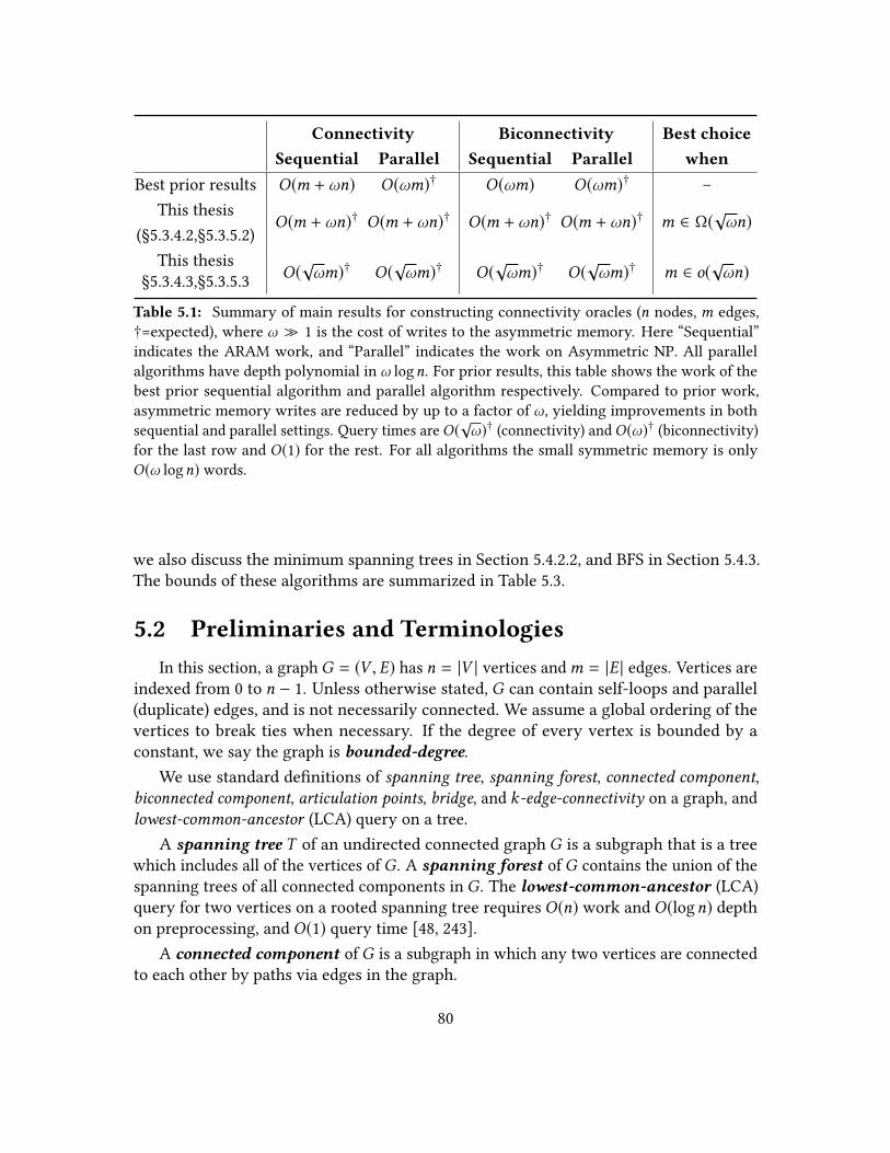
Connectivity Biconnectivity Best choice

Sequential Parallel Sequential Parallel when

Best prior results O(m + ωn) O(ωm)† O(ωm) O(ωm)† –This thesis

O(m + ωn)† O(m + ωn)† O(m + ωn)† O(m + ωn)† m ∈ Ω(√ωn)

(§5.3.4.2,§5.3.5.2)This thesis

§5.3.4.3,§5.3.5.3 O(√ωm)† O(

√ωm)† O(

√ωm)† O(

√ωm)† m ∈ o(

√ωn)

Table 5.1: Summary of main results for constructing connectivity oracles (n nodes, m edges,†=expected), where ω 1 is the cost of writes to the asymmetric memory. Here “Sequential”indicates the ARAM work, and “Parallel” indicates the work on Asymmetric NP. All parallelalgorithms have depth polynomial in ω logn. For prior results, this table shows the work of thebest prior sequential algorithm and parallel algorithm respectively. Compared to prior work,asymmetric memory writes are reduced by up to a factor of ω, yielding improvements in bothsequential and parallel settings. Query times are O(

√ω)† (connectivity) and O(ω)† (biconnectivity)

for the last row and O(1) for the rest. For all algorithms the small symmetric memory is onlyO(ω logn) words.

we also discuss the minimum spanning trees in Section 5.4.2.2, and BFS in Section 5.4.3.The bounds of these algorithms are summarized in Table 5.3.

5.2 Preliminaries and Terminologies

In this section, a graph G = (V , E) has n = |V | vertices andm = |E | edges. Vertices areindexed from 0 to n − 1. Unless otherwise stated, G can contain self-loops and parallel(duplicate) edges, and is not necessarily connected. We assume a global ordering of thevertices to break ties when necessary. If the degree of every vertex is bounded by aconstant, we say the graph is bounded-degree.

We use standard denitions of spanning tree, spanning forest, connected component,biconnected component, articulation points, bridge, and k-edge-connectivity on a graph, andlowest-common-ancestor (LCA) query on a tree.

A spanning tree T of an undirected connected graph G is a subgraph that is a treewhich includes all of the vertices of G . A spanning forest of G contains the union of thespanning trees of all connected components in G. The lowest-common-ancestor (LCA)query for two vertices on a rooted spanning tree requires O(n) work and O(logn) depthon preprocessing, and O(1) query time [48, 243].

A connected component of G is a subgraph in which any two vertices are connectedto each other by paths via edges in the graph.

80

Problem Cost and work on (M,ω)-ARAM

Single-sourceshortest paths

Q(n,m) = O(min

(n(ω +

m

M

),ω(m + n logn),m(ω + logn)

))W (n,m) = O(Q(n,m) + n logn)

Minimumspanning tree

Q(n,m) = O(m min

( nM, logn

)+ ωn

)W (n,m) = O(Q(n,m) + n logn)

Table 5.2: Summary of results on sequential graph algorithms in this thesis on the (M,ω)-ARAM.

Problem Work on Asymmetric NP Depth

MST (parallel KKT) Q(n,m) =W (n,m) =O(α(n)m + ωn log(min(m/n,ω)))

O(ω polylog(n))

Breadth-rst search Q(n,m) =W (n,m) = O(m + ωn) O(ω∆ logn) whp

Table 5.3: Summary of results on parallel graph algorithms in this thesis on the Asymmetric NP.∆ is the diameter of the input graph.

A biconnected component (also known as a block or 2-connected component) of Gis a maximal subgraph such that it is still connected after removing any single vertex inthe subgraph. Any connected graph decomposes into a tree of biconnected componentscalled the block-cut tree of the graph. The blocks are attached to each other at sharedvertices called articulation points.

A bridge of G is an edge whose deletion increases the number of connected com-ponents of the graph. A connected graph is k-edge-connected if it remains connectedwhenever fewer than k edges are removed. An unconnected graph is 0-edge connected;a connected graph with bridges is 1-edge-connected; and a bridge-less graph is at least2-edge-connected.

When G = (V , E) is a weighted graph, the edge lengths are denoted as l : E → R+.The shortest-path distance on the graph G is denoted as dG(u,v) between nodes u andv in V . Throughout this thesis, we assume that minx,y d(x,y) = 1. Let ∆ = maxx ,y d(x,y)

minx,y d(x,y) =

maxx,y d(x,y), the diameter of the graph G.

81

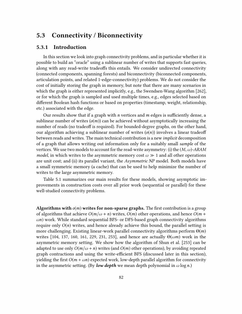
5.3 Connectivity / Biconnectivity

5.3.1 Introduction

In this section we look into graph connectivity problems, and in particular whether it ispossible to build an “oracle” using a sublinear number of writes that supports fast queries,along with any read-write tradeos this entails. We consider undirected connectivity(connected components, spanning forests) and biconnectivity (biconnected components,articulation points, and related 1-edge-connectivity) problems. We do not consider thecost of initially storing the graph in memory, but note that there are many scenarios inwhich the graph is either represented implicitly, e.g., the Swendsen-Wang algorithm [262],or for which the graph is sampled and used multiple times, e.g., edges selected based ondierent Boolean hash functions or based on properties (timestamp, weight, relationship,etc.) associated with the edge.

Our results show that if a graph with n vertices andm edges is suciently dense, asublinear number of writes (o(m)) can be achieved without asymptotically increasing thenumber of reads (no tradeo is required). For bounded-degree graphs, on the other hand,our algorithm achieving a sublinear number of writes (o(n)) involves a linear tradeobetween reads and writes. The main technical contribution is a new implicit decompositionof a graph that allows writing out information only for a suitably small sample of thevertices. We use two models to account for the read-write asymmetry: (i) the (M,ω)-ARAMmodel, in which writes to the asymmetric memory cost ω 1 and all other operationsare unit cost; and (ii) its parallel variant, the Asymmetric NP model. Both models havea small symmetric memory (a cache) that can be used to help minimize the number ofwrites to the large asymmetric memory.

Table 5.1 summarizes our main results for these models, showing asymptotic im-provements in construction costs over all prior work (sequential or parallel) for thesewell-studied connectivity problems.

Algorithms with o(m)writes for non-sparse graphs. The rst contribution is a groupof algorithms that achieve O(m/ω + n) writes, O(m) other operations, and hence O(m +ωn) work. While standard sequential BFS- or DFS-based graph connectivity algorithmsrequire only O(n) writes, and hence already achieve this bound, the parallel setting ismore challenging. Existing linear-work parallel connectivity algorithms perform Θ(m)writes [104, 137, 160, 161, 229, 231, 253], and hence are actually Θ(ωm) work in theasymmetric memory setting. We show how the algorithm of Shun et al. [253] can beadapted to use only O(m/ω +n) writes (and O(m) other operations), by avoiding repeatedgraph contractions and using the write-ecient BFS (discussed later in this section),yielding the rst O(m +ωn) expected work, low-depth parallel algorithm for connectivityin the asymmetric setting. (By low depth we mean depth polynomial in ω logn.)

82

For biconnectivity, the standard output is an array of size m indicating to whichbiconnected component each edge belongs [108, 183]. Producing this output requiresat leastm writes, and as a result, the sequential time (and parallel work) ends up beingΘ(ωm) in the asymmetric memory setting. We present an equally eective representationof the output, which we call the BC labeling, which has size only O(n). This leads to asequential biconnectivity algorithm that constructs the oracle in only O(m + ωn) time inthe asymmetric setting. Moreover, we show how to leverage our new parallel connectivityalgorithm to compute the BC labeling in O(m/ω + n) writes, yielding the rst O(m + ωn)work parallel algorithm for biconnectivity in the asymmetric memory setting. We show:

Theorem 5.3.1. Graph connectivity and biconnectivity oracles can be constructed in parallelwith O(m + ωn) expected work and O(ω2 log2 n) depth whp on the Asymmetric NP model,and each query can be answered in O(1) work. The symmetric memory is O(ω logn) words.

Algorithms with o(n) writes for sparse graphs. For sparse graphs, the work of ourconnectivity and biconnectivity algorithms is dominated by the Ω(n) writes they perform.This led us to explore the following fundamental question: Is it possible to construct,using o(n) writes to the asymmetric memory, an oracle for graph connectivity (orbiconnectivity) that can answer queries in time independent of n? Given that thestandard output for these problems (even with BC labeling) is Θ(n) size even for bounded-degree graphs, one might conjecture that Ω(n) writes are required. Our main contributionis a (perhaps surprising) armative answer to the above question for both the connectivityand biconnectivity problems.

The key technical contribution behind our breaking of the Ω(n)-write “barrier” isthe denition and use of an implicit k-decomposition of a graph. Informally, a k-decomposition of a graph G is comprised of a subset S of the vertices, called centers, and amapping ρ(·) that partitions the vertices among the centers, such that (i) |S | = O(n/k), (ii)the number of vertices in each partition is at most k , and (iii) for each center, the inducedsubgraph on its vertices is connected. However, explicitly storing the center associatedwith each vertex would require Ω(n) writes. Instead, an implicit k-decomposition denesthe mapping implicitly in terms of a procedure that is given only G and S (and a 1-bitlabeling on S).

With the new concept of implicit k-decomposition, we present three algorithmic sub-routines which together construct connectivity and biconnectivity oracles with O(m/

√ω)

writes, which is o(n) whenm ∈ o(√ωn). For clarity of presentation, we begin by assuming

the input graph has bounded degree. Section 5.3.6 discusses how to relax this constraint.We rst present an algorithm to compute an implicit k-decomposition that can be

constructed in only O(n/k) writes, O(kn) reads, and low depth, and can compute ρ(v) inonly O(k) expected reads and no asymmetric memory writes. The intuition behind ourconstruction is rst to pick a random subset of the vertices and then map each unpickedvertex to the closest center by performing a BFS on the graph G . Unfortunately, this does

83

not satisfy the constraint on partition size, so a more sophisticated approach is needed.The unique challenge that arises again and again in the asymmetric context is that thesublinear limitation on the number of writes rules out the approaches used by prior work.

We then show how the implicit k-decomposition can be used to solve graph con-nectivity and biconnectivity. We dene the concept of a clusters graph, which containsvertices each representing a cluster and edges between clusters. The key idea is that afterprecomputing on the clusters graph and storing a constant amount of information aboutconnectivity and biconnectivity on each vertex (corresponding to a cluster in the originalgraph), a connectivity or biconnectivity query can be answered by only looking at thelocal structure and preprocessed information on a constant number of clusters. This isstraightforward for connectivity queries because we need only compare the labels of theclusters that contains the respective query points. However, this becomes much morechallenging in graph biconnectivity since the correspondence between the clusters andbiconnected components is non-trivial: a cluster may contain the vertices in many bicon-nected components while the vertices in a certain biconnected component can belong todierent clusters. Therefore, biconnectivity queries require considerable subtleties in thedesign, to store the appropriate information on the clusters graph that enables each queryto access only a constant number of clusters (at most 3). More specically, we dene theconcept of the local graph of each cluster (it maintains the relationship of biconnectivityof this cluster and its neighbor clusters and can be computed with the cost proportionalto the size of this cluster), such that the biconnectivity queries discussed in Section 5.3.5can be answered by looking up a constant number of local graphs and the informationstored in the clusters graph.

Our sequential algorithms have signicant algorithmic merits on their own, but wealso show that all the algorithms can be made to run in parallel with low depth. We show:

Theorem5.3.2. Graph connectivity and biconnectivity oracles can be constructed inO(m/√ω)

expected writes andO(m√ω)work on the (M,ω)-ARAMmodel. The depth on the Asymmetric

NP is O(ω3/2 log3 n) whp. Each connectivity query can be answered in O(ω1/2) expectedtime (work) (O(ω1/2 logn) whp) and each biconnectivity query inO(ω) expected time (work)(O(ω logn) whp). The symmetric memory is O(ω logn) words.

5.3.2 Related Work

Although graph decompositions with various properties have been shown to be quiteuseful in a large variety of applications (e.g., [1, 33, 34, 35, 63, 201, 216]), to our knowledgenone of the prior algorithms provide the necessary conditions for processing graphswith a sublinear number of writes in order to answer connectivity/biconnectivity queries(targeting instead other decomposition properties that are unnecessary in our setting, suchas few edges between clusters). For example, Miller et al.’s [216] parallel low-diameterdecomposition algorithm requires at least Ω(n) writes (even if a write-ecient BFS isused), and provides no guarantees on the partition sizes. Similarly, algorithms for size-

84

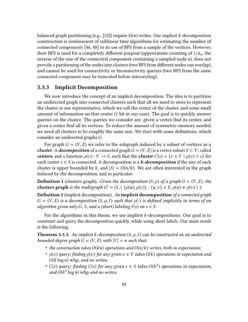
balanced graph partitioning (e.g., [22]) require Ω(n) writes. Our implicit k-decompositionconstruction is reminiscient of sublinear time algorithms for estimating the number ofconnected components [46, 88] in its use of BFS from a sample of the vertices. However,their BFS is used for a completely dierent purpose (approximate counting of 1/nu , theinverse of the size of the connected component containing a sampled node u), does notprovide a partitioning of the nodes into clusters (two BFS from dierent nodes can overlap),and cannot be used for connectivity or biconnectivity queries (two BFS from the sameconnected component may be truncated before intersecting).

5.3.3 Implicit Decomposition

We now introduce the concept of an implicit decomposition. The idea is to partitionan undirected graph into connected clusters such that all we need to store to representthe cluster is one representative, which we call the center of the cluster, and some smallamount of information on that center (1 bit in our case). The goal is to quickly answerqueries on the cluster. The queries we consider are: given a vertex nd its center, andgiven a center nd all its vertices. To reduce the amount of symmetric-memory needed,we need all clusters to be roughly the same size. We start with some denitions, whichconsider an undirected graphs G.

For graph G = (V , E) we refer to the subgraph induced by a subset of vertices as acluster. A decomposition of a connected graphG = (V , E) is a vertex subset S ⊂ V , calledcenters, and a function ρ(v) : V → S , such that the cluster C(s) = v ∈ V | ρ(v) = s foreach center s ∈ S is connected. A decomposition is a k-decomposition if the size of eachcluster is upper bounded by k , and |S | = O(n/k). We are often interested in the graphinduced by the decomposition, and in particular:Denition 1 (clusters graph). Given the decomposition (S, ρ) of a graph G = (V , E), theclusters graph is the multigraph G′ = (S, 〈 ρ(u), ρ(v) : u,v ∈ E, ρ(u) , ρ(v) 〉 ).Denition 2 (implicit decomposition). An implicit decomposition of a connected graphG = (V , E) is a decomposition (S, ρ, `) such that ρ(·) is dened implicitly in terms of analgorithm given only G, S , and a (short) labeling `(s) on s ∈ S .

For the algorithms in this thesis, we use implicit k-decompositions. Our goal is toconstruct and query the decomposition quickly, while using short labels. Our main resultis the following.Theorem 5.3.3. An implicit k-decomposition (S, ρ, `) can be constructed on an undirectedbounded-degree graph G = (V , E) with |V | = n such that:

• the construction takes O(kn) operations and O(n/k) writes, both in expectation;• ρ(v) query: nding ρ(v) for any given v ∈ V takesO(k) operations in expectation andO(k logn) whp, and no writes;

• C(s) query: nding C(s) for any given s ∈ S takes O(k2) operations in expectation,and O(k2 logn) whp and no writes;

85

d

h

j i c

f

k al

g

e

bPrimary center

Secondary center

Figure 5.1: An example implicit k-decomposition for k = 4 consisting of clustersd,h, l, i, j,b, e, f , and a, c,д,k. In the graph, j ′s primary center is e (i.e., ρ0(j) = e) and itssecondary center is b (i.e., ρ(j) = b). Note b is on the shortest path to from j to e . Also note that cis closer to the secondary center b than to д, but picks д as its actual center, because b is not on theshortest path to its primary center. In breaking ties we assume lexicographically smaller lettershave higher priorities. The solid lines are on shortest paths from a vertex to its secondary center.

• the labels `(s), s ∈ S are 1-bit each; and,• construction and queries take O(k logn) symmetric memory whp.

Note that this theorem indicates a linear tradeo between reads (operations) and writesfor the construction controlled by k .

At a high level, the construction algorithm works by identifying a subset of centerssuch that every vertex can quickly nd its nearest center without having to keep a pointerto it (which would require too many writes). It rst selects a random subset of the verticeswhere each vertex is selected with probability 1/k . We call these the primary centersand denote them as S0. All other vertices are then assigned to the nearest such center.Unfortunately, a cluster dened in this way can be signicantly larger than k (super-polynomial in k). To handle this, the algorithm identies an additional O(n/k) secondarycenters, S1. Every vertex v is associated with a primary center ρ0(v) ∈ S0, and an actualcenter ρ(v) ∈ S = S0 ∪ S1. The only values the algorithm stores are the set S and thebits `(s), s ∈ S indicating whether it is primary or secondary. An example is given inFigure 5.1.

In our construction it is important to break ties among equal-length paths in a consis-tent way, such that subpaths of a shortest path are themselves a unique shortest path. Forthis purpose we assume the vertices have a total ordering (and comparing two verticestakes constant time). Among two equal hop-length paths from a vertex u, consider therst vertex where the paths diverge. We say that the path with the higher priority vertexat that position is shorter. Let SP(u,v) be the shortest path between u and v under thisdenition for breaking ties, and L(SP(u,v)) be its length such that comparing L(SP(u,v))and L(SP(u,w)) breaks ties as dened. By our denition all subpaths of a shortest path

86

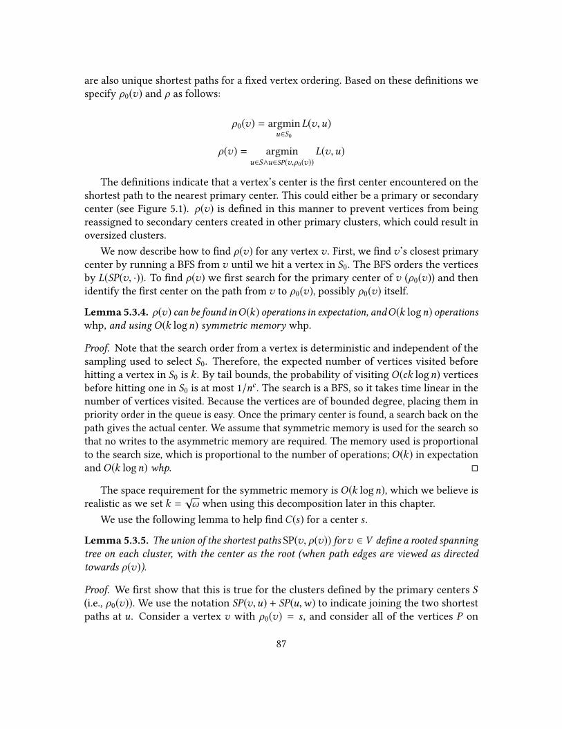
are also unique shortest paths for a xed vertex ordering. Based on these denitions wespecify ρ0(v) and ρ as follows:

ρ0(v) = argminu∈S0

L(v,u)

ρ(v) = argminu∈S∧u∈SP(v,ρ0(v))

L(v,u)

The denitions indicate that a vertex’s center is the rst center encountered on theshortest path to the nearest primary center. This could either be a primary or secondarycenter (see Figure 5.1). ρ(v) is dened in this manner to prevent vertices from beingreassigned to secondary centers created in other primary clusters, which could result inoversized clusters.

We now describe how to nd ρ(v) for any vertex v . First, we nd v’s closest primarycenter by running a BFS from v until we hit a vertex in S0. The BFS orders the verticesby L(SP(v, ·)). To nd ρ(v) we rst search for the primary center of v (ρ0(v)) and thenidentify the rst center on the path from v to ρ0(v), possibly ρ0(v) itself.

Lemma5.3.4. ρ(v) can be found inO(k) operations in expectation, andO(k logn) operationswhp, and using O(k logn) symmetric memory whp.

Proof. Note that the search order from a vertex is deterministic and independent of thesampling used to select S0. Therefore, the expected number of vertices visited beforehitting a vertex in S0 is k . By tail bounds, the probability of visiting O(ck logn) verticesbefore hitting one in S0 is at most 1/nc . The search is a BFS, so it takes time linear in thenumber of vertices visited. Because the vertices are of bounded degree, placing them inpriority order in the queue is easy. Once the primary center is found, a search back on thepath gives the actual center. We assume that symmetric memory is used for the search sothat no writes to the asymmetric memory are required. The memory used is proportionalto the search size, which is proportional to the number of operations; O(k) in expectationand O(k logn) whp.

The space requirement for the symmetric memory is O(k logn), which we believe isrealistic as we set k =

√ω when using this decomposition later in this chapter.

We use the following lemma to help nd C(s) for a center s .

Lemma 5.3.5. The union of the shortest paths SP(v, ρ(v)) forv ∈ V dene a rooted spanningtree on each cluster, with the center as the root (when path edges are viewed as directedtowards ρ(v)).

Proof. We rst show that this is true for the clusters dened by the primary centers S(i.e., ρ0(v)). We use the notation SP(v,u) + SP(u,w) to indicate joining the two shortestpaths at u. Consider a vertex v with ρ0(v) = s , and consider all of the vertices P on

87

the shortest path from v to s . The claim is that for each u ∈ P, ρ(u) = s and SP(u, s) isa subpath of P . This implies a rooted tree. To see that ρ(u) = s note that the shortestpath from u to a primary vertex t has length L(SP(u, t)). We can write the length ofthe shortest path from v to t as L(SP(v, t)) ≤ L(SP(v,u) + SP(u, t)) and the length of theshortest path from v to s as L(SP(v, s)) = L(SP(v,u) + SP(u, s)). Because ρ0(v) = s , weknow that L(SP(v, s)) < L(SP(v, t)) ∀t , s . Through substitution and subtraction, we seethat L(SP(u, s)) < L(SP(u, t)) ∀t , s . This means that ρ0(u) = s . We know that SP(u, s)cannot contain the edge b that v takes to reach u in SP(v, s) because u ∈ SP(v, s). Sincethe search from u excluding b will have the same priorities as the search from v when itreaches u, SP(u, s) is a subpath of P .

Now consider the clusters dened by ρ(v). The secondary centers associated with aprimary center s partition the tree for s into subtrees. Each subtree begins (relative tothe root) at a center and ends when encountering another center (this other center isnot included). Each vertex in the tree for s will be assigned the correct partition by ρ(v)because each will be assigned to the rst secondary center on the way to the primarycenter.

The set of solid edges in Figure 5.1 is an example of the spanning forest. This givesthe following.

Corollary 5.3.6. For any vertex v , SP(v, ρ(v)) ⊆ C(ρ(v)).

Lemma 5.3.7. For any vertex s ∈ S , its clusterC(s) can be found inO(k |C(s)|) operations inexpectation and O(k |C(s)| logn) operations whp, and using O(|C(v)| + k logn) symmetricmemory whp.

Proof. For any center s ∈ S , identifying all the vertices in its cluster C(s) can be imple-mented as a BFS starting at s . For each vertex v ∈ V that the BFS visits, the algorithmchecks if ρ(v) = s . If so, we add v toC(s) and put its unvisited neighbors in the BFS queue,and otherwise we do neither. By Corollary 5.3.6, any vertex v for which ρ(v) = s musthave a path to s only through other vertices whose center is v . Therefore the algorithmwill visit all vertices in C(s). Furthermore, because the graph has bounded degree itwill only visit O(C(s)) vertices not in C(s). Each visit to a vertex u requires nding ρ(v).Our bound on the number of operations therefore follows from Lemma 5.3.4. We useO(|C(v)|) symmetric memory for storing the queue andC(v), andO(k logn)memory whpfor calculating ρ(v).

We now show how to select the secondary centers such that the size of each clusteris at most k . Algorithm 4 describes the process. By Lemma 5.3.5, before the secondarycenters are added, each primary vertex in s ∈ S0 denes a rooted tree of paths from thevertices in its cluster to s . The function SecondaryCenters then recursively cuts up thistree into subtrees rooted at each u that is identied.

88

Algorithm 4: Constructing Implicit k-DecompositionInput: Connected bounded-degree graph G = (V , E), parameter kOutput: A set of cluster centers S0 and S1 (S = S0

⋃S1)

1 Sample each vertex with probability 1/k , and place in S02 S1 =

3 foreach vertex v ∈ S0 do

4 SecondaryCenters(v , G, S0)5 return S0 and S1

6 function SecondaryCenters(v , G, S)7 Search from v for the rst k vertices that have v as their center. This denes a

tree.8 If the search exhausts all vertices with center v , return.9 Otherwise identify a vertex u that partitions the tree such that its subtree and

the rest of the tree are each at least a constant fraction of k .10 Add u to S1.11 SecondaryCenters(v , G, S ∪ u)12 SecondaryCenters(u, G, S ∪ u)

Lemma 5.3.8. Algorithm 4 runs inO(nk) operations andO(n/k)writes (both in expectation),and uses O(k logn) symmetric memory whp on the (M,ω)-ARAM Model. It generates aimplicit k-decomposition S of G with labels distinguishing S0 from S1.

Proof. The algorithm creates clusters of size at most k by construction (it partitions anycluster bigger thank using the added verticesu). Each call to SecondaryCenters (withoutrecursive calls) will use O(k2) operations in expectation because we visit k vertices andeach one has to search back tov to determine ifv is its center. Each call also usesO(k logn)space for the search whp because we need to store the k elements found so far and eachρ(v) uses O(k logn) space for the search whp. Before making the recursive calls, we writeout u to S1, requiring one write per call to SecondaryCenters. The symmetric memorycan be reused by the recursive calls.

We are left with showing there are at mostO(n/k) calls to SecondaryCenters. Thereare n/k primary centers in expectation. If there are too many (beyond some constantfactor above the expectation), we can try again. Because the graph has bounded degree,we can nd a vertex that partitions the tree such that its subtree and the rest of the treeare both at most a constant fraction of k . We can now charge all internal nodes of therecursion against the leaves. There are at most O(n/k) leaves because each denes acluster of size Θ(k). Therefore there are O(n/k) calls to SecondaryCenters, giving thestated overall bounds.

89

Parallelizing the decomposition. To parallelize the decomposition in Algorithm 4, wemake one small change; in addition to adding u to the set of secondary centers at eachrecursive call to SecondaryCenters, we add all children of v (thus separating v into itsown cluster). This guarantees that the height of the tree decreases by at least one on eachrecursive call, and only increases the number of writes by a constant factor. This givesthe following lemma.

Lemma 5.3.9. On the Asymmetric NP model, Algorithm 4 runs in depth O(k3 log2 n) whp.

Proof. Certainly selecting the set S0 can be done in parallel. Furthermore the calls toSecondaryCenters on line 4 can be made recursively in parallel. The depth will beproportional to the depth to each call to SecondaryCenters (not including recursivecalls) multiplied by the depth of the recursion. To bound the depth, in the parallel versionwe also mark the children of the root as secondary centers, which does not increase thenumber of secondary centers asymptotically (due to the bounded-degree assumption). Inthis way the height of the tree decreases by one on each recursive call. The depth of therecursion is at most the depth of the tree associated with the primary center ρ0(v). This isbounded by O(k logn) whp because by Lemma 5.3.4 every vertex nds its primary centerwithin O(k logn) steps whp. The depth of SecondaryCenters (without recursion) is justthe number of operations (O(k2 logn) whp). This gives the bound.

Extension to unconnected graphs. Note that once a connected component containsat least one primary center, the denition and Theorem 5.3.3 hold. However, it is possiblethat in a small component, the search of ρ(·) exhausts all connected vertices withoutnding any primary centers (vertices in the initial sample, S0). In this case, we checkwhether the size of the cluster is at least k , and if so, we mark as a primary center thevertex that is the smallest according to the total order on vertices. This marks at mostn/k primary centers and the rest of the algorithm remains unchanged. This step is addedafter line 1 in Algorithm 4, and requires O(nk) work and operations, O(n/k) writes, andO(k + logn) depth. The cost bound therefore is not changed. If the component is smallerthan k , we use the smallest vertex in the component as a center implicitly, but never writeit out. The ρ(·) function can easily return this in O(k) operations.

5.3.4 Graph Connectivity and Spanning Forest

This section describes parallel write-ecient algorithms for graph connectivity andspanning forest; that is, identifying which vertices belong to each connected componentand producing a spanning forest of the graph. These tasks can be easily accomplishedsequentially by performing a breadth-rst or depth-rst search in the graph with O(m)operations and O(n) writes. While there are several work-ecient parallel algorithmsfor the problem [104, 137, 160, 161, 229, 231, 253], all of them use Ω(n +m) writes. Thissection has two main contributions: (1) Section 5.3.4.2 provides a parallel algorithm usingO(n +m/ω) writes in expectation, O(nω +m) expected work, and O(ω2 log2 n) depth with

90

high probability; (2) Section 5.3.4.3 gives an algorithm for constructing a connectivityoracle on constant-degree graphs in O(n/

√ω) expected writes and O(n

√ω) expected total

operations. Our oracle-construction algorithm is parallel, having depth O(ω3/2 log3 n)whp, but it also represents a contribution as a sequential algorithm.

Our parallel algorithm (Section 5.3.4.2) can be viewed as a write-ecient versionof the parallel algorithm due to Shun et al. [253]. This algorithm uses a low-diameterdecomposition algorithm of Miller et al. [216] as a subroutine, which we review and adaptnext in Section 5.3.4.1.

The exponential distribution with parameter λ is dened by the probability densityfunction:

f (x, λ) =

λe−λx if x ≥ 00 otherwise

The mean of the exponential distribution is 1/λ.

5.3.4.1 Low-diameter Decomposition

Here we review the low-diameter decomposition of Miller et al. [216]. The so-called“(β,d)-decomposition” is terminology lifted from their paper, and it should not be confusedwith our implicit k-decompositions. The details of the decomposition subroutine areimportant only to extract a bound on the number of writes.

A (β,d)-decomposition of an undirected graph G = (V , E), where 0 < β < 1 and1 ≤ d ≤ n, is dened as a partition of V into subsets V1, . . . ,V` such that (1) the shortestpath between any two vertices in each Vi using only vertices in Vi has length at most d ,and (2) the number of edges (u,v) ∈ E crossing the partition, i.e., such that u ∈ Vi , v ∈ Vj ,and i , j, is at most βm. Miller et al. [216] provide a parallel algorithm for generatinga (β,O(logn/β))-decomposition with O(m) operations and O((log2 n)/β) depth whp. Asdescribed by Miller et al., the number of writes performed is also O(m), but this can beimproved to O(n). Specically, the algorithm executes multiple breadth-rst searches(BFS’s) in parallel, which can be replaced by write-ecient BFS’s.

In more detail, the algorithm rst assigns each vertex v a value δv drawn from anexponential distribution with parameter β (mean 1/β). Then on iteration i of the algorithm,BFS’s are started from unexplored vertices v where δv ∈ [i, i + 1) and all BFS’s that havealready started are advanced one level. At the end of the algorithm, all vertices thatwere visited by a BFS starting from the same source will belong to the same subsetof the decomposition. If a vertex is visited by multiple BFS’s in the same iteration, itcan be assigned to an arbitrary BFS.1 The maximum value of δv can be shown to beO(logn/β) whp, and so the algorithm terminates in O(logn/β) iterations. Each iteration

1The original analysis of Miller et al. [216] requires the vertex to be assigned to the BFS with the smallerfractional part of δs , where s is the source of the BFS. However, Shun et al. [253] show that an arbitraryassignment gives the same complexity bounds.

91

requires O(logn) depth for packing the frontiers of the BFS’s, leading to an overall depthof O(log2 n/β) whp. A standard BFS requires operations and writes that are linear in thenumber of vertices and edges explored, giving a total work of O(ω(m + n)). By using thewrite-ecient BFS, the expected number of writes for each BFS is proportional to thenumber of vertices marked (assigned to it), and so the total expected number of writes isO(n). Tasks only needO(1) symmetric memory in the algorithm. This yields the followingtheorem:

Theorem 5.3.10. A (β,O(logn/β))-decomposition can be generated inO(n) expected writes,O(m + ωn) expected work, and O(log2 n/β) depth whp on the Asymmetric NP model.

5.3.4.2 Connectivity and Spanning Forest

The parallel connectivity algorithm of [253] applies the low-diameter decompositionrecursively with β set to a constant less than 1. Each level of recursion contracts a subsetof vertices into a single supervertex for the next level. The algorithm terminates wheneach connected component is reduced to a single supervertex. The stumbling block forwrite eciency is this contraction step, which performs writes proportional to the numberof remaining edges.

Instead, our write-ecient algorithm applies the low-diameter decomposition justonce, but with a much smaller β , as follows:

1. Perform the low-diameter decomposition with parameter β = 1/ω + n/m.2. Find a spanning tree on each Vi (in parallel) using write-ecient BFS.3. Create a contracted graph, where each vertex subset in the decomposition is con-

tracted down to a single vertex. To write down the cross-subset edges in a compactedarray, employ the write-ecient lter (Section 4).

4. Run any parallel linear-work spanning forest algorithm on the contracted graph,e.g., the algorithm from [104] with O(ω logn) depth.

Combining the spanning forest edges across subsets (produced in Step 4) with the spanningtree edges (produced in Step 2) gives a spanning forest on the original graph. Adding thebounds for each step together yields the following theorem. Again only O(1) symmetricmemory is required per task.

Theorem 5.3.11. For any choice of 0 < β < 1, connectivity and spanning forest can besolved in O(n + βm) expected writes, O(ωn + βωm +m) expected work, and O(log2 n/β)depth whp on the Asymmetric NP model. For β = 1/ω, these bounds reduce to O(n +m/ω)expected writes, O(m + ωn) expected work and O(minω,m/n log2 n) depth whp.

Proof. Step 1 has performance bounds given by Theorem 5.3.10, and the expected numberof edges remaining in the contracted graph is at most βm. Step 2 performs BFS’s ondisjoint subgraphs, so summing across subsets yieldsO(n) expected writes andO(m +nω)expected work. Since each tree has low diameter D = O(logn/β), the BFS’s have depth

92

O(D logn) = O(log2 n/β) whp (Section 5.4.3). Step 3 is dominated by the lter, which hasa number of writes proportional to the output size of O(βm), for O(m + βωm) work. Thedepth is O(logn) (Section 4.2.2). Finally, the algorithm used in Step 4 is not write-ecient,but the size of the graph is O(n + βm), giving that many writes and O(ω(n +mβ)) work.Adding these bounds together yields the theorem.

5.3.4.3 Connectivity Oracle in Sublinear Writes

A connectivity oracle supports queries that take as input a vertex and return the label(component ID) of the vertex. This allows one to determine whether two vertices belongin the same component. The algorithm is parameterized by a value k , to be chosen later.We assume throughout that the symmetric memory per task is Ω(k logn) words and thatthe undirected graph has bounded degree.

We begin with an outline of the algorithm. The goal is to produce an oracle that cananswer for any vertex which component it belongs to inO(k)work. To build the oracle, wewould like to run the connectivity algorithm on the clusters graph produced by an implicitk-decomposition. The result would be that all center vertices in the same componentbe labeled with the same identier. Answering a query then amounts to outputting thecomponent ID of the center it maps to, which can be queried in O(k) expected work andO(k logn) work whp according to Lemma 5.3.4.

The main challenge in implementing this strategy is that we cannot aord to writeout the edges of the clusters graph (as there could be too many edges). Instead, we treatthe implicit k-decomposition as an implicit representation of the clusters graph. Given animplicit representation, our connected components algorithm is the following:

1. Find an implicit k-decomposition of the graph.2. Run the write-ecient connectivity algorithm from Section 5.3.4.2 with β = 1/k ,

treating the k-decomposition as an implicit representation of the clusters graph, i.e.,querying edges as needed.

As used in the connectivity algorithm, our implicit representation need only be ableto list the edges in the clusters graph that are adjacent to a center vertex x . To do so, startat x , and explore outwards (e.g., with BFS), keeping all vertices and edges encountered sofar in symmetric memory. For each frontier vertex v , query its center (as in Lemma 5.3.7)— if ρ(v) = x , then v’s unexplored neighbors are added to the next frontier; otherwise (ifρ(v) , x ) the edge (x, ρ(v)) is in the clusters graph, so add it to the output list.

Lemma 5.3.12. Assuming a symmetric memory of size Ω(k logn), the centers neighboringeach center in the clusters graph can be listed in no writes, and work, depth, and operationsall O(k2) in expectation or O(k2 logn) whp.

Proof. Listing all the vertices in the cluster takes expected work O(k2) according toLemma 5.3.7, or O(k2 logn) whp. The number of vertices in the cluster is O(k), so theycan all t in symmetric memory. Moreover, because each vertex in the cluster has O(1)

93

neighbors, the total number of explored vertices in neighboring clusters is O(k), all ofwhich can t in symmetric memory. Each of these vertices is queried with a cost of O(k)operations in expectation and O(k logn) whp given the specied symmetric memory size(Lemma 5.3.4).

Note that a consequence of the implicit representation is that listing neighbors is moreexpensive, and thus the number of operations performed by a BFS increases, aecting boththe work and the depth. The implicit representation is only necessary while operatingon the original clusters graph, i.e., while nding the low-diameter decomposition andspanning trees of each of those vertex subsets; the contracted graph can be built explicitlyas before. The best choice of k is k =

√ω, giving us the following theorem.

Theorem 5.3.13. A connectivity oracle that answers queries in O(√ω) expected work and

O(√ω logn) work whp can be constructed in O(n/

√ω) expected writes, O(

√ωn) expected

work, and O(ω3/2 log3 n) depth whp on the Asymmetric NP model, assuming a symmetricmemory of size Ω(

√ω logn).

Proof. The implicit k-decomposition can be found in O(n/k) writes, O(kn + ωn/k) work,and O(k3 log2 n) depth by Lemmas 5.3.8 and 5.3.9. For k =

√ω, these bounds reduce to

O(n/√ω) writes, O(

√ωn) work, and O(ω3/2 log3 n) depth.

If we had an explicit representation of the clusters graph with n′ = O(n/k) vertices andm′ = O(m) = O(n) edges, the connectivity algorithm would have O(n′ +m′/k) = O(n/k)expected writes, O(ωn′ + ωm′/k +m′) = O(ωn/k + n) expected work, and O(k log2 n)depth whp (by Theorem 5.3.11). The fact that the clusters graph is implicit means thatthe BFS needs to perform O(k2) additional work (but not writes) per node in the clustersgraph, giving expected workO(ωn/k +n+k2n′) = O(ωn/k +kn). To get a high probabilitybound, the depth is multiplied by O(k2 logn), giving us O(k3 log3 n) = O(ω3/2 log3 n) fork =√ω.

We can also output the spanning forest on the contracted graph in the same bounds,which will be used in the biconnectivity algorithms in Sections 5.3.5.3 and 5.3.5.4.

5.3.5 Graph Biconnectivity

In this section we introduce algorithms related to biconnectivity and 1-edge connec-tivity queries. We rst review the classic approach and its output, which requires Θ(m)writes. Then we propose a new BC (biconnected-component) labeling output, which hassize O(n) and can be constructed in O(n) writes. Queries such as determining bridges,articulation points, and biconnected components can be answered in O(1) operations(and no writes) with the BC labeling. Finally we show how an implicit k-decomposition(as generated by Algorithm 4) can be integrated into the algorithm to further reduce thewrites to O(n/

√ω).

94

We begin by presenting sequential algorithms that we believe to be new and interesting.Then in Section 5.3.5.4 we show that these algorithms are parallelizable. All of ourbiconnectivity algorithms use O(k logn) symmetric memory.

In this section we assume that the graph is connected. If not, we can run the connec-tivity algorithm and then run the algorithm on each component. The results for a graphare the union of the results of each of its connected components.

5.3.5.1 The Classic Algorithm

The classic Tarjan-Vishkin parallel algorithm [266] to compute biconnected com-ponents and bridges of a connected graph is based on the Euler-tour technique. Thealgorithm starts by building a spanning tree T rooted at some arbitrary vertex. Eachvertex is labeled by rst(v) and last(v), which are the ranks ofv’s rst and last appearanceon the Euler tour of T . The low value low(v) and the high value high(v) of a vertex v ∈ Vare dened as:

low(v) = minw(u) | u is in the subtree rooted at vhigh(v) = maxw(u) | u is in the subtree rooted at v

wherew(u) = minrst(u) ∪ rst(u′) | (u,u′) is a nontree edge2

Namely, low(v) and high(v) indicate the rst and last vertex on the Euler tour thatare connected by a nontree edge to the subtree rooted at v . The low(·) and high(·) valuescan be computed by a reduce on each vertex followed by a leax3 on the subtrees. Thecomputation of low and high takesO(logn) depth,O(m+ωn)work, andO(n)writes on theAsymmetric NP model, by using the algorithm and scheduling theorem in Chapter 2 and 4.Then a tree edge is a bridge if and only if the child’s low and high is inclusively within therange of rst and last values of its parent. The cost of this variant of the Tarjan-Vishkinalgorithm applied to nding bridges is dominated by the cost of the spanning tree, asgiven in Theorem 5.3.11.

For biconnected components, the standard output is an array B[·] of sizem, where the i-th element in B indicates to which biconnected component the i-th edge belongs [108, 183].Explicitly writing out B is costly in the asymmetric setting, especially whenm n. Weprovide an alternative BC labeling as output that requires only O(n) writes.

5.3.5.2 The BC Labeling

Here we describe the BC (biconnected-component) labeling, which eectively rep-resents biconnectivity output in O(n) space. Instead of storing all edges within eachbiconnected component, the BC labeling stores a component label for each vertex, and a

2If there are multiple edges (u,u ′) in the graph, none of them are considered here.3Leax is similar to prex but dened on a tree and computed from the leaves to the root.

95

1

2 6

3 4 5 7 8 9

Figure 5.2: An example of the BC labeling of a graph. The spanning tree is rooted at vertex 1. Thesolid and dot lines indicate tree edges while dot lines are the critical edges. Dash lines are non-treeedges. The vertex labels l = [1, 1, 1, 2, 1, 1, 3, 3] (note that the root does not have a label), and compo-nent heads r = [1, 2, 6]. Based on the BC labeling the bridges, articulation points, and biconnectedcomponents can be easily retrieved as (2, 5), 2, 6, and 1, 2, 3, 4, 6, 7, 2, 5, 6, 8, 9.

vertex for each component. An example of a BC labeling of a graph is shown in Figure 5.2.We will later show how to use this representation along with an implicit decompositionto reduce the writes further.

Denition 3 (BC labeling). The BC labeling of a connected undirected graph with respectto a rooted spanning tree stores a vertex label l : V \root → [C] where C is the numberof biconnected components in the graph, and a component head r : [C] → V of eachbiconnected component.

Lemma 5.3.14. The BC labeling of a connected graph can be computed in O(m) operationsand O(n +m/ω) writes on the (M,ω)-ARAM. Queries to nd bridges, articulation points,or biconnected components can be answered in no writes and O(1) operations given a BClabeling on a rooted spanning tree.

The algorithm to compute BC labeling. A vertex v ∈ V (except for the root) is anarticulation point if and only if there exists at least one child u in the spanning tree thathas rst(v) ≤ low(u) and high(u) ≤ last(v), and here we call the tree edge between such apair of vertices a critical edge. The algorithm to compute the BC labeling simply removesall critical edges and runs graph connectivity on all remaining graph edges. Then thealgorithm described in Section 5.3.4.2 gives a unique component label that we assignas the vertex label. For each component, its head is the vertex that is its parent in thespanning tree (this parent is unique). Each connected component and its head form abiconnected component.

The correctness of the algorithm can be proven by showing the equivalence of theresult of this algorithm and that of the Tarjan-Vishkin algorithm [266].

96

Because the number of biconnected components is at most n, the spanning tree, vertexlabels, and component heads require only linear space. Therefore, the space requirementof the BC labeling is O(n).

Query on BC labeling. We now show that queries are easy with the BC labeling. Anedge is a bridge if and only if it is the only edge connecting a single-vertex componentand its component head (the biconnected component contains this single edge). The rootof the spanning tree is an articulation point if and only if it is the head of at least twobiconnected components. Any other vertex is an articulation point if and only if it is thehead of at least one biconnected component. A block-cut tree can also be generated fromthe BC labeling: for each vertex create an edge from itself and its vertex label; and foreach component create an edge from the label of this component to the component head.We have a block-cut tree after removing degree-1 nodes corresponding to vertices.

This new representation can be interpreted as an implicit version of the standardoutput [108, 183] of biconnected components, i.e., the label of the biconnected componentof each edge can be reported in O(1) operations. This is simple: we report the label of theendpoint of the edge that is further from the root along the spanning tree. The correctnesscan be shown in two cases: if the edge is a spanning tree edge, then the component labelis stored in the further vertex; otherwise, the two vertices must have the same label andreporting either one gives the label of this biconnected component.

Using BC labeling gives the following theorem (see Section 5.3.5.4 for depth analysis):

Theorem 5.3.15. Articulation points, bridges, and biconnected components on the Asym-metric NP model takeO(m +nω) expected work andO(minω,m/n log2 n) depth whp, andeach query can be answered in O(1) work.

It is interesting to point out that, the BC labeling can eciently answer queries thatare non-trivial when using the standard output. For example, consider the query: aretwo vertices in the same biconnected component? With the BC labeling we can answerthe query by nding the label of the lower vertex and checking whether the higherone has the same label or is the component head of this component. To the best of ourknowledge, answering such queries on the standard representation can be hard, unlessother information is also kept (e.g. a block-cut tree).

5.3.5.3 Biconnectivity Oracle in Sublinear Writes

Next we will show how the implicit k-decomposition generated by Algorithm 4 canbe integrated into the algorithm to further reduce writes in the case of bounded-degreegraphs. Our goal is as follows.

Theorem 5.3.16. There exists an algorithm that computes articulation points, bridges, andbiconnected components of a bounded-degree graph in O(n

√ω) expected work, O(n/

√ω)

97

writes andO(ω3/2 log3 n) depth, and each query takes an expectedO(ω) work andO(ω logn)work whp, with no writes, on the Asymmetric NP model.

The overall idea of the new algorithm is to replace the vertices in the original graphwith the clusters generated by Algorithm 4. We generate the BC labeling on the clustersgraph (so the vertex labels are now the cluster labels), and then show that a biconnectivityquery can be answered using only the information on the clusters graph and a constantnumber of associated clusters. The cost analysis is based on the parameter k , and usingk =√ω gives the result in the theorem.

The BC labeling on the clusters graph.

In the rst step of the algorithm we generate the BC labeling on the clusters graphwith k =

√ω. We root this spanning tree and name it the clusters spanning tree. The head

vertex of a cluster is chosen as the cluster root for that cluster. (The root cluster does nothave a cluster root.) For a cluster, we call the endpoint of a cluster tree edge outside of thecluster an outside vertex. The outside vertices of a cluster is the set of outside verticesof all associated cluster tree edges. Note that all outside vertices except for one are thecluster roots for neighbor clusters.

The local graph of a cluster.

We next dene the concept of the local graph of a cluster, so that each query onlyneeds to look up a constant number of associated local graphs. An example of a localgraph is shown in Figure 5.3 and a more formal denition is as follows.

Denition 4 (local graph). The local graph G′ of a cluster is dened as (Vi ∪Vo, E′), whereVi is the set of vertices in the cluster and Vo is the set of outside vertices, and E′ consists of:

1. The edges with both endpoints in this cluster and the associated clusters’ tree edges.

2. For c neighbor clusters sharing the same cluster label, we nd the c correspondingoutside vertices in Vo , and connect the vertices with c − 1 edges.

3. For an edge (v1,v2) with only one endpoint v1 in Vi , we nd the outside vertex vo thatis connected to v2 on the cluster spanning tree, and create an edge from v1 to vo .

Figure 5.3 shows an example local graph. Solid black lines are edges within the clusterand solid grey lines are cluster tree edges. Neighbor clusters that share a label are shownwith dashed outlines and connected via curved dashed lines. e1 and e2 are examples ofedges with only one endpoint in the cluster, and they are replaced by e′1 and e′2 respectively.

Computing local graphs requires a spanning tree and BC labeling of the clusters graph.

Lemma 5.3.17. The cost to construct one local graph isO(k2) in expectation andO(k2 logn)whp on the (M,ω)-ARAM.

Proof. Each cluster in the implicit k-decomposition has at most k vertices, so nding thevertices Vi takes O(ck) cost where c is the cost to compute the mapping ρ(·) of a vertex

98

𝑒1

𝑒1′

𝑒2′

𝑒2

Figure 5.3: An example of a local graph. The vertices in the shaded area is in one cluster. Thelocal graph contains the vertices in the shaded area and the outside vertices shown in smallercircles. Solid lines indicate the edges that are in the clusters and thick grey lines represent clustertree edges connecting other clusters (which are shown in yellow pentagons). The three neighborclusters sharing the same cluster label are connected using two edges (dash curves). Edges e1 ande2 are the edges that only has one endpoints in the cluster. The other endpoint is set to be theoutside vertex connecting the cluster of the other original endpoint of this edge in the clusterspanning tree. Consequently e ′1 and e ′2 are the replaced edges for e1 and e2.

99

Algorithm 5: Sublinear-write algorithm for biconnectivityInput: Connected bounded-degree graph G = (V , E) and an implicit

k-decomposition

1 Apply connectivity algorithm to generate the clusters graph.2 Compute low(·) and high(·) values of all clusters.3 Compute the BC labeling of the clusters graph.// Bridges and articulation points can be queried

4 Compute the root biconnectivity of all outside vertices in all local graphs.5 Apply leax to identify the articulation point of each cluster root.// Biconnectivity and 1-edge connectivity on vertices and edges can be queried

6 Compute the number of biconnected components in each cluster that arecompletely within this cluster.

7 Apply prex sums on the clusters to give an identical label to each biconnectedcomponent.

// The label of biconnected component can be queried

(O(k) in expectation and O(k logn) whp). Since each vertex has a constant degree, therewill be at most O(k) neighbor clusters, so |Vo | = O(k). Enumerating and checking theother endpoint of the edges adjacent to Vi takes O(ck) cost. Finding the new endpoint ofan edge in category 3 requires constant cost after an O(n/k) preprocessing of the Eulertour of the cluster spanning tree. The number of neighbor clusters isO(k) so checking thecluster labels and adding edges costs no more thanO(k). The overall cost to construct onelocal graph is thus O(k2) in expectation and O(k2 logn) whp. After plugging in c is O(k)in expectation and O(k logn) whp, the overall cost matches the bounds in the lemma.

Queries.

With the local graph and the BC labeling on the clusters graph, many types of bicon-nectivity queries can be answered. Some of them are easier while other queries requiremore steps, and the preprocess steps are shown in an overview of Algorithm 5.

Bridges. There are three cases when deciding whether an edge is a bridge: a tree edgein the clusters spanning tree, a cross edge in the clusters spanning tree, or an edge withboth endpoints in the same cluster. Deciding which case to use takes constant operations.

A tree edge is a bridge if and only if it is a bridge of the clusters graph, which wecan mark with O(n/k) writes while computing the BC labeling. A cross edge cannot be abridge.

For an edge within a cluster, we use the following lemma:

Lemma 5.3.18. An edge with both endpoints in one cluster is a bridge if and only if it is abridge in the local graph of the corresponding cluster.

100

Proof. If an edge is a bridge in the original graph it means that there are no edges fromthe subtree of the lower vertex to the outside except for this edge itself. By applying themodications of the edges, this property still holds, which means the edge is still a bridgein the local graph and vice versa.

Checking if an edge in a cluster is a bridge takes O(k2) work in expectation andO(k2 logn) whp.

Articulation points. By a similar argument, a vertex is an articulation point of theoriginal graph if and only if it is an articulation point of the associated local graph. Givena query vertexv , we can check whether it is an articulation point the local graph associatedto v , which costs O(k2) work in expectation and O(k2 logn) whp.

We now discuss how to perform several more complex queries. To start with, we showsome denitions and results that are used in the algorithms for queries.

Denition 5 (root biconnectivity). We say a vertex v in a cluster C’s local graph is root-biconnected if v and the cluster root have the same vertex label in C’s local graph.

A root-biconnected vertex v indicates that v can connect to the ancestor clusterswithout using the cluster root (i.e., the cluster root is not an articulation point to cut v).Another interpretation is that there is no articulation point in cluster C that disconnectsv from the outside vertex of the cluster root.

Lemma 5.3.19. Computing and storing the root biconnectivity of all outside vertices in alllocal graphs takes O(nk) operations in expectation and O(n/k) writes on the (M,ω)-ARAM.

The proof is straightforward. The cost to construct the local graphs and compute rootbiconnectivity is O(nk), and since there are O(n/k) clusters tree edges, storing the resultsrequires O(n/k) writes.

Querying whether two vertices are biconnected. Checking whether two vertices v1and v2 can be disconnected by removing any single vertex in the graph is one of the mostcommonly-used biconnectivity-type queries. To answer this query, our goal is to nd thetree path between this pair of vertices and check whether there is an articulation point onthis path that disconnects them.

The simple case is when v1 and v2 are within the same cluster. We know that the twovertices are connected by a path via the vertices within the cluster. We can check whetherany vertex on the path disconnects these two vertices using their vertex labels.

Otherwise, v1 and v2 are in dierent clusters C1 and C2. Assume CLCA is the clusterthat contains the LCA of v1 and v2 (which can be computed by the LCA of C1 and C2 inO(1) operations) and vLCA ∈ CLCA is the LCA vertex. The tree path between v1 and v2 isfromv1 toC1’s cluster root, and then to the cluster root of the outside vertex ofC1’s clusterroot, and so on, until reaching vLCA, and the other half of the path can be constructed

101

symmetrically. It takesO(k2) expected operations to check whether any articulation pointdisconnects the paths inC1,C2 andCLCA. For the rest of the clusters, since we have alreadyprecomputed and stored the root biconnectivity of all outside vertices, then applying aleax on the clusters spanning tree computes the cluster containing the articulation pointof each cluster root. Therefore, checking whether such an articulation point exists onthe path between C1 and CLCA or between C2 and CLCA that disconnects v1 and v2 takesO(1) operations. Thus, checking whether two vertices are biconnected requires O(k2)

operations in expectation and no writes.

Querying whether two vertices are 1-edge connected. This is a similar query com-paring to the previous one and the only dierence is whether an edge, instead of a vertex,is able to disconnect two vertices. The query can be answered in a similar way by check-ing whether a bridge disconnects the two vertices on their spanning tree path, which isrelated to the two clusters containing the two query vertices and the LCA cluster, andthe precomputed information for the clusters on the tree path among these three clusters.The cost for a query is also O(k2) operations in expectation and it requires no writes.

Queries on biconnected-component labels for edges. We now answer the standardqueries [108, 183] of biconnected components: given an edge, report a unique label thatrepresents the biconnected component this edge belongs to.

We have already described the algorithm to check whether any two vertices arebiconnected, so the next step is to assign a unique label of each biconnected components,which requires the following lemma:

Lemma 5.3.20. A vertex in one cluster is either in a biconnected component that onlycontains vertices in this cluster, or biconnected with at least one outside vertex of this cluster.

Proof. Assume a vertex v1 in this cluster C is biconnected to another vertex v2 outsidethe cluster, then let vo be the outside vertex of C on the spanning tree path between v1and v2, and v1 is biconnected with vo , which proves the lemma.

With this lemma, we rst compute and store the labels of the biconnected componentson the cluster roots, which can be nished with O(nk) expected operations and O(n/k)writes with the BC labeling on the clusters graph and the root biconnectivity of outsidevertices on all clusters. Then for each cluster we count the number of biconnectedcomponents completely within this cluster. Finally we apply a prex sum on the numbersfor the clusters to provide a unique label of each biconnected component in every cluster.Although not explicitly stored, the vertex labels in each cluster can be regenerated withO(k2) operations in expectation andO(k2 logn) operations whp, and a vertex label is eitherthe same as that of an outside vertex which is precomputed, or a relative label within thecluster plus the oset of this cluster.

Similar to the algorithm discussed in Section 5.3.5.2, when a query comes, the edgecan either be a cluster tree edge, a cross edge, or within a cluster. For the rst case the

102

label biconnected component is the precomputed label for the (lower) cluster root. Forthe second case we just report the vertex label of an arbitrary endpoint, and similarly forthe third case the output is the vertex label of the lower vertex in the cluster. The cost ofa query is O(k2) in expectation and O(k2 logn) whp.

With the concepts and lemmas in this section, with a precomputation of O(nk) costand O(n/k) writes, we can also do a normal query with O(k2) cost in expectation andO(k2 logn) whp on bridge-block tree, cut-block tree, and 1-edge-connected compo-

nents.

5.3.5.4 Parallelizing Biconnectivity Algorithms

The two biconnectivity algorithms discussed in this section are highly parallelizable.The key algorithmic components include Euler-tour construction, tree contraction, graphconnectivity, prex sum, and preprocessing LCA queries on the spanning tree. Since thealgorithms run each of the components a constant number of times, the depth of thealgorithm is bounded by the depth of graph connectivity, whose bound is provided inSection 5.3.4 (O(ω2 log2 n) and O(ω3/2 log3 n) whp when plugging in β as 1/ω and 1/

√ω,

respectively).4

For the sublinear-write algorithm, we assume that computations within a clusterare sequential, and the work is upper bounded by O(k2) = O(ω) in expectation andO(k2 logn) = O(ω logn) whp for the computations within a cluster. This term is additiveto the overall depth, since after computing the spanning tree (forest) of the clusters, werun all computations within the clusters in parallel and then run tree contraction andprex sums based on the calculated values. The O(ω) expected work (O(ω logn) whp)is also the cost for a single biconnectivity query, and multiple queries can be done inparallel.

5.3.6 Sublinear-Write Algorithms on Unbounded-Degree Graphs

Here we discuss a solution to generate another graph G′ which has bounded degreewith O(m) vertices and edges, and the connectivity queries on the original graph G canbe answered in G′ equivalently.

The overall idea is to build a tree structure with virtual nodes for each vertex thathas more than a constant degree. Each virtual node will represent a certain range of theedge list. Considering a star with all other vertices connecting to a specic vertex v1, webuild a binary tree structure with 2 virtual nodes on the rst level v1,2→n/2, v1,n/2+1→n,4 virtual nodes on the second level v1,2→n/4, · · · ,v1,3n/4+1→n and so on. We replace theendpoint of an edge from the original graph G with the leaf node in this tree structure

4The classic parallel algorithms with polylogarithmic depth solve the Euler-tour construction, treecontraction, and prex sum, since we here only require linear writes (in terms of number of vertices, O(n)and O(n/k), for the two algorithms) for both algorithms.

103

that represents the corresponding range with a constant number of edges. Notice that ifboth endpoints of an edge have large degrees, then they both have to be redirected.

The simple case is for a sparse graph in which most of the vertices are bounded-degree,and the sum of the degrees for vertices with more than a constant number of edges isO(n/k) (or O(n/

√ω)). In this case we can simply explicitly build a tree structure for the

edges of a vertex.Otherwise, we require the adjacency array of the input graph to have the following

property: each edge can query its positions in the edge lists for both endpoints. Namely,an edge (u,v) knows it is the i-th edge in u’s edge list and j-th edge in v’s edge list. Toachieve this, either an extra pointer is stored for each edge, or the edge lists are presortedand the label can be binary searched (this requires O(logn) work for each edge lookup).With this information, there exists an implicit graph G′ with bounded-degree. The binarytree structures can be dened such that given an internal tree node, we can nd the threeneighbors (two neighbors for the root) without explicitly storing the newly added verticesand edges. Notice that the new graphG′ now hasO(m) vertices including the virtual ones.The virtual nodes help to generate implicit k-decomposition and require no writes unlessthey are selected to be either primary or secondary centers.

Graph connectivity is obviously not aected by this transformation. It is easy to checkthat a bridge in the original graph G is also a bridge in the new graph G′ and vice versa.In the biconnectivity algorithm, an edge in G can be split into multiple edges in G′, butthis will not change the biconnectivity property within a biconnected component, unlessthe component only contains one bridge edge, which can be checked separately.

This construction, combined with our earlier results, leads to Theorem 5.3.2.

5.3.7 Conclusion

This work provides several algorithms targeted at solving graph connectivity problemsconsidering the read-write asymmetry. Our algorithms make use of an implicit decompo-sition technique that is applicable beyond the scope of the problems studied in this thesis.By using this decomposition and redundantly performing small computation, we are ableto reduce the number of writes in exchange for a small increase in the total number ofoperations. This allows us to oset the increased cost of writes in anticipated futuresystems and improve overall performance. Even excluding new memory technology, webelieve that research into algorithms with fewer writes provides interesting results fromboth a theoretical and memory/cache coherence perspective. Our work provides a frame-work which can be used to develop write-ecient solutions to large graph connectivityproblems.

104

5.4 Distance-based Algorithms

On (M,ω)-ARAM model, breadth-rst and depth-rst search can be performed withQ =W = O(ωn +m). In particular each vertex only requires a constant number of writeswhen it is rst added to the frontier (the stack or queue) and a constant number of writeswhen it is nished (removed from the stack or queue). Searches along an edge to analready visited vertex requires no writes. This implies that several problems based on BFSand DFS also only requireQ =W = O(DFS(n)). For example, topological sort, biconnectedcomponents, and strongly connected components. The analysis is based on the fact thatthere are onlyO(n) forward edges in the DFS. However when using priority-rst search ona weighed graph (e.g., Dijkstra’s or Prim’s algorithms) then the problem is more dicultto perform optimally. This is because the priority queue might need to be updated forevery edge that is visited. A common theme in many of our algorithms is that they useredundant computations and require a tradeo between reads and writes. We show howto adapt Dijkstra’s single-source shortest-paths algorithm using phases so that the priorityqueue is kept in small-memory (Section 5.4.1), and briey sketch how to adapt Borůvka’sminimum spanning tree algorithm to reduce the number of shortcuts and hence writesthat are needed (Section 5.4.2).

For parallel and write-ecient graph algorithms, we show minimum spanning trees inSection 5.4.2.2, and BFS in Section 5.4.3. The parallelism is from the random exponentialgrowing-with-ltering technique.

5.4.1 Single-Source Shortest Paths

The single-source shortest-paths (SSSP) problem takes a directed weighted graphG = (V , E) and a source vertex s ∈ V , and outputs the shortest distances d(s,v) from sto every other vertex in v ∈ V . For graphs with non-negative edge weights, the mostecient algorithm is Dijkstra’s algorithm [114].

In this section we will study (variants of) Dijkstra’s algorithm in the asymmetricsetting. We describe and analyze three versions (two classical and one new variant) ofDijkstra’s algorithm, and the best version can be chosen based on the values of M , ω, thenumber of vertices n = |V |, and the number of edgesm = |E |.

Theorem 5.4.1. The SSSP problem on a graph G = (V , E) with non-negative edge weightscan be solvedwithQ(n,m) = O

(min

(n(ω +

m

M

),ω(m + n logn),m(ω + logn)

))andW (n,m) =

O(Q(n,m) + n logn), both in expectation, on the (M,ω)-ARAM.

We start with the classical Dijkstra’s algorithm [114], which maintains for each vertexv , δ (v), a tentative upper bound on the distance, initialized to +∞ (except for δ (s), whichis initialized to 0). The algorithm consists of n − 1 iterations, and the nal distances froms are stored in δ (·). In each iteration, the algorithm selects the unvisited vertex u withsmallest nite δ (u), marks it as visited, and uses its outgoing edges to relax (update) all of

105

its neighbors’ distances. A priority queue is required to eciently select the unvisitedvertex with minimum distance. Using a Fibonacci heap [128], the work of the algorithmis O(m + n logn) in the standard (symmetric) RAM model. In the (M,ω)-ARAM, the costsare Q = W = O(ω · (m + n logn)) since the Fibonacci heap requires asymptotically asmany writes as reads. Alternatively, using a binary search tree for the priority queuereduces the number of writes (see Section 4.1) at the cost of increasing the number ofreads, giving Q =W = O(m logn + ωm). These bounds are better when m = o(ωn). Bothof these variants store the priority queue in large-memory, requiring at least one write tolarge-memory per edge.

We now describe an algorithm, which we refer to as phased Dijkstra, that fully main-tains the priority queue in small-memory and only requires O(n) writes to large-memory.The idea is to partition the computation into phases such that for a parameter M′ eachphase needs a priority queue of size at most 2M′ and visits at least M′ vertices. By selectingM′ = M/c for an appropriate constant c , the priority queue ts in small-memory, and theonly writes to large-memory are the nal distances.

Each phase starts and ends with an empty priority queue P and consists of two parts.A Fibonacci heap is used for P , but is kept small by discarding the M′ largest elements(vertex distances) whenever |P | = 2M′. To do this P is attened into an array, the M′-thsmallest element dmax is found by selection, and the Fibonacci heap is reconstructed fromthe elements no greater than dmax , all taking linear time. All further insertions in a givenphase are not added to P if they have a value greater than dmax . The rst part of each phaseloops over all edges in the graph and relaxes any that go from a visited to an unvisitedvertex (possibly inserting or decreasing a key in P ). The second part then runs the standardDijkstra’s algorithm, repeatedly visiting the vertex with minimum distance and relaxingits neighbors until P is empty. To implement relax, the algorithm needs to know whethera vertex is already in P , and if so its location in P so that it can do a decrease-key on it.It is too costly to store this information with the vertex in large-memory, but it can bestored in small-memory using a hash table.

The correctness of this phased Dijkstra’s algorithm follows from the fact that it onlyever visits the closest unvisited vertex, as with the standard Dijkstra’s algorithm.

Lemma 5.4.2. Phased Dijkstra’s hasQ(n,m) = O(n(ω +

m

M

))andW (n,m) = O(Q(n,m)+

n logn) both in expectation (forM ≤ n).

Proof. During a phase either the size of P will grow to 2M′ (and hence delete someentries) or it will nish the algorithm. If P grows to 2M′ then at least M′ vertices arevisited during the phase since that many need to be deleted with delete-min to emptyP . Therefore the number of phases is at most dn/M′e. Visiting all edges in the rst partof each phase involves at mostm insertions and decrease-keys into P , each taking O(1)amortized time in small-memory, and O(1) time to read the edge from large-memory.Since compacting Q when it overows takes linear time, its cost can be amortized against

106

the insertions that caused the overow. The cost across all phases for the rst part istherefore Q =W = O(mdn/M′e). For the second part, every vertex is visited once andevery edge relaxed at most once across all phases. Visiting a vertex requires a delete-minin small-memory and a write to large-memory, while relaxing an edge requires an insertor decrease-key in small-memory, and O(1) reads from large-memory. We therefore havefor this second part (across all phases) that Q = O(ωn +m) andW = O(n(ω + logn) +m).The operations on P each include an expected O(1) cost for the hash table operations.Together this gives our bounds.

Compared to the rst two versions of Dijkstra’s algorithm with Q =W = O(ωm +min(ωn logn,m logn)), the new algorithm is strictly better when ωM > n. More speci-cally, the new algorithm performs better when nm/M < maxωm,min(ωn logn,m logn).Combining these three algorithms proves Theorem 5.4.1, when the best one is chosenbased on the parameters M , ω, n, andm.

We will discuss the implementation details of Phased Dijkstra later in Section 8.6.2.

5.4.2 Minimum Spanning Tree (MST)

In this section we discuss several commonly-used algorithms for computing a min-imum spanning tree (MST) on a weighted graph G = (V , E) with n = |V | vertices andm = |E | edges. Some of them are optimal in terms of the number of writes (O(n)). Al-though loading a graph into large-memory requires O(m) writes, the algorithms are stilluseful on applications that compute multiple MSTs based on one input graph. For example,it can be useful for computing MSTs on subgraphs, such as road maps, or when edgeweights are time-varying functions and hence the graph maintains its structure but theMST varies over time.

Prim’s algorithm. All three versions of Dijkstra’s algorithm discussed in Section 5.4.1can be adapted to implement Prim’s algorithm [108]. Thus, the upper bounds of ARAMcost and work in Theorem 5.4.1 also hold for minimum spanning trees.

Kruskal’s algorithm. The initial sorting phase requires Q = W = O(m logn + ωm)(Section 4.4.1). The second phase constructs a MST using union-nd without path com-pression in O(m logn) work, and performs O(n) writes (the actual edges of the MST).Thus, the complexity is dominated by the rst phase. Neither ARAM cost nor work matchour variant of Borůvka’s algorithm.

5.4.2.1 Borůvka’s Algorithm

Borůvka’s algorithm consists of at most logn rounds. Initially all vertices belong intheir own component, and in each round, the lightest edges that connect each componentto another component are added to the edge set of the MST, and components are mergedusing these edges. This merging can be done using, for example, depth rst searchamong the components and hence takes time proportional to the number of remaining

107

components. However, since edges are between original vertices the algorithm is requiredto maintain a mapping from vertices to the component they belong to. Shortcutting allvertices on each round to point directly to their component requiresO(n)writes per roundand hence up to O(n logn) total writes across the rounds. This is not a bottleneck in thestandard RAM model but is in the asymmetric case.

We now describe a variant of Borůvka’s algorithm which is asymptotically optimalin the number of writes. It requires only O(1) small-memory. The algorithm proceeds intwo phases. For the rst log logn rounds, the algorithm performs no shortcuts (beyondthe merging of components). Thus it will leave chains of length up to log logn that needto be followed to map each vertex to the component it belongs to. Since there are at mostO(m log logn) queries during the rst log logn rounds and each only require reads, thetotal work for identifying the minimum edges between components in the rst phase isO(m(log logn)2). After the rst phase all vertices are shortcut to point to their component.We refer to these components as the phase-one components. In the second phase, onevery round, we shortcut the phase-one components to point directly to the componentthey belong to. Since there can only be at most n/logn phase-one components, and atmost logn − log logn rounds in phase-two, the total number of reads and writes for theseupdates is O(n). During phase two the mapping from a vertex to its component takes twosteps: one to nd its phase-one component and another to get to the current component.Therefore the total work for identifying the minimum edges between components in thesecond phase is O(m logn).

All other work is on the components themselves (i.e., adding the forest of minimumedges and performing DFS to merge components). The number of reads, writes, and otherinstructions is proportional to the number of components. There are n components onthe rst round and the number decreases by at least a factor of two on each followinground. Therefore the total work on the components is O(ωn). Summing the costs give thefollowing lemma.

Lemma 5.4.3. Our variant of Borůvka’s algorithm generates a minimum spanning treeon a graph with n vertices andm edges with ARAM cost and work Q(n,m) = W (n,m) =O(m logn + ωn) on the (M,ω)-ARAM.

Theorem 5.4.4. A minimum spanning tree on a graph G = (V , E) can be computed withARAM costQ(n,m) = O

(m min

( nM, logn

)+ ωn

)and workW (n,m) = O(Q(n,m)+n logn)

on the (M,ω)-ARAM.

The theorem is a combination of the bounds of Prim’s and Borůvka’s algorithms (then/M term is in expectation).

5.4.2.2 KKT Algorithm and the Parallel Version

This section extends Karger, Klein and Tarjan’s (KKT) [185] sequential linear-workrandomized algorithm for minimum spanning tree/forest. At a high level, their algorithm

108

proceeds as follows: Randomly sample half of the edges, and calculate a minimum spanningforest on these sampled edges. Use the sampled forest to lter out edges that cannot bepart of the overall minimum spanning forest. Specically, identify all edges e = (x,y)of the graph such that e is the heaviest edge on the cycle it closes in the sampled forest.These edges are discarded. Next, recurse on the remaining graph and perform a constantnumber “Borůvka steps” to reduce the number of nodes in the graph. The proof that thisalgorithm runs in linear work hinges on two main facts: rst, that the ltering can be donein linear work, and second, that the number of edges ltered out is large in expectation.We will use the following denitions in this section.

Denition 6. For a given treeT in the graph, and two vertices x,y ∈ V , the path connectingx and y in T (if such a path exists) is denoted by τ (x,y).

Denition 7. An edge e = (x,y) is said to be heavy with respect to a treeT on the graph ife closes a cycle in T and it is the heaviest edge in that cycle. That is,w(e) ≥ max(w(e′) | e′ ∈τ (x,y)). Any edge that is not heavy with respect to T is said to be light with respect to T .

Recall the well-known cycle property of MSTs: a tree T is an MST in a graph G if andonly if every non-tree edge closes a cycle in T and is the maximum weight edge on thatcycle. Therefore, if all edges of a graph not inT are heavy, thenT is an MST of that graph.

The ltering-out of heavy edges is achieved via minimum spanning tree vericationalgorithms. These algorithms take a tree and a graph as input and determine whether thetree is an MST in the graph. They operate by labeling each edge as light or heavy withrespect to the tree. There is extensive work on the verication of minimum spanningtrees, and several algorithms are known to operate in linear work [116, 159, 188]. TheKKT algorithm then throws out any edges labelled heavy by the verication algorithm,and recurses on the remainder of the graph.

To be ecient, the KKT algorithm requires that when a minimum spanning forest isbuilt on a random subset of the graph, a large fraction of edges in the remaining graphcan be ltered out. They show that this holds using the following lemma:5

Lemma 5.4.5 (Sampling Lemma). For a random subset R ⊆ E of size r , and a randomsubset S ⊆ E of size s , the expected number of edges in S that are light with respect to theMST of R is less than sn/r .

Using this lemma, Karger et al. prove that their algorithm requires O(m) work with highprobability.

Write-ecient MST.

Our goal is to nd an MST algorithm that minimizes the number of writes performedwithout signicantly increasing the number of reads. A slight modication of Borůvka’s

5The statement of this lemma is a slight variation of the version given in [86] and is dierentfrom the original paper [185].

109

Algorithm 6: Write-ecient MST algorithmInput: A graph G = (V , E)Output: An MST with a set T of edges

1 sampleSize← max(2n,m/ω)2 Edge set T ← 3 while sampleSize < m do

4 The set of light edges SL ← 5 for s ← 1 to sampleSize do6 Randomly pick an edge e ∈ E7 if e cannot be ltered with respect to T then

8 SL ← SL + e

9 T ← KKT(SL ∪T )10 sampleSize← 2 · sampleSize11 SL ← 12 forall e ∈ E do // Take all edges in nal round13 if e cannot be ltered with respect to T then

14 SL ← SL + e

15 T ← KKT(SL ∪T )16 return T

algorithm yields an algorithm which executes inO(m logn+ωn)work in the (M,ω)-ARAMmodel. That is, we can achieve the optimal number of writes (O(n)) usingO(m logn) reads.However, we want to nd an algorithm that more closely matches the optimal work ofthe algorithm of Karger et al. [185].

We present an MST algorithm that uses the KKT algorithm as a subroutine, and requiresO(α(n)m) reads (where α(·) is the inverse Ackermann function) andO(n log(min(m/n,ω)))writes, resulting in O(α(n)m + ωn log(min(m/n,ω))) work.

The algorithm is iterative, and proceeds as follows. It begins by taking an O(n) sizedrandom sample of the edges and running KKT on them to nd a minimum spanning forestof the sampled graph. Then, in each round, it takes a random sample that is twice as largeas the previous one, lters out the edges in the sample that are heavy with respect to themost recently calculated spanning forest, and then runs KKT again on the remaining partof the sample. In each such round, with high probability, we will only be left with O(n)edges from the sample that pass the ltering, and so each round will need O(n) writes.The algorithm proceeds in this way until the nal sample includes all edges in the graph.The pseudocode for this algorithm is presented in Algorithm 6.

Analysis.

110

We start with a sample set S of edges with size max(2n,m/ω), and run the KKTalgorithm on this sample to calculate a minimum spanning forest on it. We then doublethe size of the sample set in each round and recalculate, until all edges are processed.However, to save writes, instead of storing all the samples, we use an online lteringalgorithm to throw out the edges that are heavy, and only keep the light sample edges.We sample slightly (a constant factor) more than our desired sample size to account forcollisions. Note that once the sample size is linear in m, we can sample by ipping a coinwith appropriate probabilities for each edge, without increasing the algorithm’s total work.We dene the edge set SL to be the subset of S that contains light edges (with respect tothe current spanning forest in this round), and the edge set SH to be the subset consistingof heavy edges. Clearly, S = SH ∪ SL.

Lemma 5.4.6. At the end of round i of the algorithm, we have a minimum spanning foreston Θ(2i−1 max(n,m/ω)) edges of the graph in expectation.

Proof. In round i , we have at least Θ(2i−1 max(2n,m/ω)) sample edges in expectation,but only build a minimum spanning forest using the edges in SL, along with the tree wealready have. Let T be the set of edges in the current forest, as shown in the pseudocode.Note that by the denition of heavy edges, T is a minimum spanning forest in the graphwhose edge set is SH ∪T . Therefore, the MST ofT ∪ SL is also a minimum spanning foreston T ∪ SL ∪ SH .

Therefore, at the end of round dlog2(min(m/n,ω))e, we have an MST on the entiregraph, and we are done. Note that in the last round, we simply consider all of the edges(without sampling) to ensure that we’ve seen every edge.

Lemma 5.4.7. In every round, the expected size of SL, the number of edges that pass theltering, is Θ(n).

Proof. By Lemma 5.4.6, the MST used to lter edges in round i is a minimum spanningforest on at least c12i−1n edges in expectation for some constant c1. The sample size inround i is c22in in expectation for some constant c2. By the Sampling Lemma, the expected

size of SL in round i is less thansn

r=c2(2in)nc12i−1n

= Θ(n).

By Lemmas 5.4.6 and 5.4.7, it is easy to see that, excluding any work needed for theltering, the total number of writes required for this algorithm is O(n log(min(m/n,ω))),and the number of reads is

∑dlog2(min(m/n,ω))ei=1 Θ(2in) = O(m).

Ideally, we would like the ltering step to take no more thanO(n)writes per round, anda constant number of reads per edge. There are several MST verication algorithms thattake work linear in the number of edges [116, 159, 188]. However, all of these algorithmsalso take O(m) writes, and are therefore not suitable for us. Alon and Schieber [18]present an online algorithm for minimum spanning tree verication that operates in O(n)

111

preprocessing work, and then α(n) work per queried edge. The queries are done througha look-up in the data structure built in the preprocessing stage, and require no writes.Using their algorithm allows us to execute the entire write-ecient MST algorithm inO(n log(min(m/n,ω))) writes and O(α(n)m) reads.

Alon and Schieber also prove a matching lower bound for the problem of answeringonline tree product queries, which is a generalization of the MST verication problem.However, they show this lower bound looking at the worst case query. It may be possibleto improve upon this result by considering the query time amortized over all of the edges.

Parallel Analysis.

We can parallelize each of the steps of the algorithm. Clearly, the sampling of edgescan be done in parallel in constant depth. We then use a parallel version of Alon andSchieber’s algorithm [18] to lter out heavy edges. This takes polylogarithmic depth.Cole et al. [104] presented a parallel version of the KKT algorithm that takes linear workand polylogarithmic depth, which we can use instead of the sequential version wheneverwe call KKT. So simply by using the parallel versions of these algorithms, we achievea work-ecient polylogarithmic depth algorithm (we only sample O(log(min(m/n,ω)))times, and the depth is only increased by a factor of O(log(min(m/n,ω)))).

However, we need to be precise with the number of writes required in the parallelversion. After using Alon and Schieber’s algorithm to check whether each sampled edgecan be ltered out, we need to pack out the edges that passed the ltering to use them inthe next round of the algorithm. A standard packing algorithm would execute a numberof writes proportional to the total size of the sample, which is too many writes for us. Forthis, we use the output sensitive lter algorithm presented in Section 4.2.2.

We thus obtain the following theorem:

Theorem 5.4.8. Given a graph G withm edges and n vertices, an MST of G can be foundinO(α(n)m +ωn log(min(m/n,ω))) work,O(polylog(n)) depth andO(n log(min(m/n,ω)))writes whp in the Asymmetric NP model, where α(·) is the inverse Ackerman function.

5.4.3 Parallel Breadth-First Search

The breadth-rst search (BFS) problem takes as input an unweighted graph G = (V , E)and a source vertex r , and returns breadth-rst search tree rooted at r containing allvertices reachable from r . This section describes a parallel write-ecient BFS algorithm.We will use the notation n = |V | andm = |E |. The standard sequential BFS algorithm iswrite-ecient, but not parallel. It requires O(m + ωn) work, including O(n) writes (theminimum number of writes required for BFS). On the other hand, the standard parallellevel-synchronous BFS algorithm of [53] is not write-ecient, requiring O(m) writes. Thealgorithm explores the graph in parallel, where round i visits all vertices at a distance iaway from r (we call the vertices newly explored in round i − 1 the frontier for roundi). Each frontier vertex visits and writes to all of its unexplored neighbors in parallel,

112

which causes additional writes when multiple frontier vertices attempt to visit the samevertex simultaneously. This algorithm uses O(ω(m + n)) work, O(∆ logn) depth whp, andO(m + n) writes, where ∆ is the diameter of the input graph.

We now present an algorithm for BFS that runs in O(m + ωn) work and O(∆ log2 n)depth using only O(n) writes in expectation. The algorithm works like level-synchronousBFS, but makes use of exponential delaying algorithm when visiting the vertices in around to reduce collisions (and writes) on a shared neighbor. In exponential delayingexploration takes place in iterations, where on each iteration we process a fraction of thevertices on the frontier. We rst randomize the order of the frontier vertices, and then onthe rst iteration we process the rst vertex and on iteration i > 1, we process the next2i−2 vertices on the frontier. During the exploration process, a vertex checks to see if itsneighbor has been visited and only updates that neighbor if it was not visited in a priorround or a prior iteration in the same round.

We now show that the number of writes for this algorithm is O(n) in expectation.Consider a vertex v that is adjacent to the current frontier and has not yet been visited.Let F be the number of vertices on the frontier (without loss of generality, assume it is apower of 2), let NF (v) be the number of in-neighbors v has on the frontier. We will useα = 1 − (NF (v)/F ) for notational convenience. The probability that v is rst visited initeration 1 is α and in iteration i > 1 is:

(1 − α2i−2)α

i−1∏j=2

α2j−2= (1 − α2i−2

)α2i−2

The expected number of vertices that attempt to visit v in iteration 1 is NF (v)/F = 1 − αand in iteration i > 1 is 2i−2(1 − α). Summing the expectations over all iterations gives:

(1 − α)α +log F∑i=2

2i−2(1 − α)(1 − α2i−2)α2i−2

< O(1) +log F∑i=2

2i−2α2i−2= O(1)

where we use∑∞

x=1 xax = O(1) for 0 ≤ a < 1. This shows that the expected number of

writes to a vertex is O(1), and the expected number of writes overall is O(n).Randomly permuting the vertices sums to linear work overall andO(log2 n) depth whp

per round [217, 254]. The logn iterations used in the exponential delaying also contributesO(∆ log2 n) to the depth per round. Thus the overall depth is O(∆ log2 n). The number ofreads remains O(m + n), which gives the following theorem.

Theorem 5.4.9. For a graph with n vertices,m edges, and diameter diam, our write-ecientbreadth-rst search algorithm requires O(m + ωn) work in expectation, O(∆ log2 n) depthwhp, and O(n) writes in expectation on the Asymmetric NP model.

113

114

Chapter 6

Geometric Algorithms

6.1 Overview

Achieving parallelism (polylogarithmic depth) and optimal write-eciency simultane-ously seems generally hard for many algorithms and data structures in computationalgeometry. This is because for most geometric algorithms, the computation is not xed, butdecided by the input value. Therefore, simple solutions to partition the computations intosmaller chunks and apply the computations within the small-memory are not available.Here, optimal write-eciency means that the number of writes that the algorithm or datastructure construction performs is asymptotically equal to the output size.

This thesis mainly consists of two general frameworks and show how they can be usedto design algorithms and data structures from geometry with high parallelism as well asoptimal write-eciency. The rst framework is designed for randomized incrementalalgorithms. Randomized incremental algorithms are relatively easy to implement inpractice, and the challenge is in simultaneously achieving high parallelism and write-eciency. There are several technical parts in this framework. The rst part includesseveral new incremental algorithms, which is the rst step of the parallel and write-ecient algorithms. The diculty of this step is usually in showing the parallelism, andin this approach the new results are based on analyzing the dependence graph of thesealgorithms. This technique is used in other problems in [61, 164, 225, 254]. The secondpart is for the write-eciency (while maintaining parallelism), which further consistsof two components: a DAG-tracing algorithm and a prex doubling technique. Thewrite-eciency is from the DAG-tracing algorithm, that given a current conguration ofa set of objects and a new object, nds the part of the conguration that “conicts” withthe new object. Finding n objects in a conguration of size n requires O(n logn) readsbut only O(n) writes. Once the conicts have been found, then previous and new parallelincremental algorithms can be used to resolve the conicts among objects taking linear

115

reads and writes. This allows for a prex doubling approach in which the number ofobjects inserted in each round is doubled until all objects are inserted.

This framework obtains parallel write-ecient algorithms for comparison sort, planarDelaunay triangulation, and k-d trees, all requiring optimal work, linear writes, andpolylogarithmic depth. The most interesting result is for Delaunay triangulation (DT).Although DT can be solved in optimal time and linear writes sequentially using the planesweep method, previous parallel DT algorithms seem hard to make write ecient. Mostare based on divide-and-conquer, and seem to inherently require Θ(n logn) writes. TheDT algorithm in this thesis requires delicate above-mentioned design and analysis inorder to achieve parallelism and write-eciency. For k-d trees, the p-batched incremen-tal construction technique is introduced that maintains the balance of the tree whileasymptotically reducing the number of writes.

The second framework is designed for augmented trees, including interval trees, rangetrees, and priority search trees. The goal is to achieve write-eciency for both the initialconstruction as well as future dynamic updates. The framework consists of two techniques.The rst technique is to decouple the tree construction from sorting, and introduce parallelalgorithms to construct the trees in linear reads and writes after the objects are sorted(the sorting in Chapter 4 can be done with linear writes). Such algorithms provide write-ecient constructions of these data structures, but can also be applied in the rebalancingscheme for dynamic updates—once a subtree is reconstructed once it is unbalanced. Thesecond technique is the α-labeling. Some tree nodes are subselected as critical nodes, andthe augmentation is only maintained on these nodes. By doing so the number of treenodes that need to be written on each update is limited, at the cost of having to read morenodes.

This framework obtains ecient augmented trees in the asymmetric setting. Inparticular, the trees can be constructed in optimal work and writes, and polylogarithmicdepth. For dynamic updates, a trade-o is provided between performing extra reads inqueries and updates, while doing fewer writes on updates. A standard algorithm usesO(logn) reads and writes per update (O(log2 n) reads on a 2D range tree). The numberof writes can be reduced by a factor of Θ(logα) for α ≥ 2, at a cost of increasing readsby at most a factor of O(α) in the worst case. For example, when the number of queriesand updates are about equal, we can improve the work by a factor of Θ(logω), which issignicant given that the update and query costs are only logarithmic.

The previous two frameworks introduce new parallel write-ecient algorithms forcomparison sorting, planar Delaunay triangulation, k-d trees, and static and dynamicaugmented trees (including interval trees, range trees and priority search trees). We believethe techniques in these frameworks will be useful for designing other algorithms in boththe symmetric and asymmetric settings. Also, new parallel write-ecient algorithmsfor write-sensitive hash tables, and sequential write-ecient algorithms for LP-stylealgorithms are also discussed in this chapter.

116

Randomized Incremental Algorithms.

The randomized incremental approach (RIC1) has been an extremely useful paradigmfor generating simple and ecient algorithms for a variety of problems. There have beendozens of papers on the topic (e.g., see the surveys [218, 248]). Much of the early workwas in the context of computational geometry, but the approach has more recently beenapplied to graph algorithms [101, 107]. The main idea is to insert elements one-by-one inrandom order while maintaining a desired structure. The random order ensures that theinsertions are somehow spread out, and worst-case behaviors are unlikely.

The incremental process is iterative, and hence would appear to be sequential andnot write-ecient. In this thesis, we proposed a framework to analyze the computationalDAG of the RIC algorithms, to show the parallelism and write-eciency together in auniform analysis.

The incremental process would appear sequential since it is iterative, but in practiceincremental algorithms are widely used in parallel implementations by allowing someiterations to start in parallel and using some form of locking to avoid conicts. Manyparallel implementations for Delaunay triangulation and convex hull, for example, arebased on the randomized incremental approach [49, 82, 98, 99, 113, 144, 202, 230, 252]. Intheory, however, after 25 years, there are still no known bounds for parallel Delaunaytriangulation using the incremental approach, nor for many other problems.

In this thesis we rst show that the incremental approach for Delaunay and manyother problem is actually parallel, at least with the right incremental algorithms, andleads to work-ecient polylogarithmic-depth (time) algorithms for the problems. Theresults are based on analyzing the dependence graph. This technique has recently beenused to analyze the parallelism available in a variety of sequential algorithms, includingthe simple greedy algorithm for maximal independent set [61], the Knuth shue forrandom permutation [254], greedy graph coloring [164], and correlation clustering [225].The advantage of this method is that one can use standard sequential algorithms withmodest change to make them parallel, often leading to very simple parallel solutions. Ithas also been shown experimentally that this approach leads to quite practical parallelalgorithms [60], and to deterministic parallelism [60, 75].

We then show the write-ecient versions of these algorithms. For sorting and Delau-nay triangulation, the number of writes is linear, which is optimal since this is the outputsize. For other linear-work algorithms, the number of writes can be bounded to O(nϵ ) forany ϵ > 0. Some analysis here.

The contributions of the section can be summarized as follows.

1The letter C is for constrcution. In early works RIC algorithms were used to construct some generalizedgeometric data structures including convex hull and triangulation. Later work, including this thesis,extended the scope of these algorithms, but we still call them RIC algorithms to follow the convention.

117

Problem Work (expected) Depth (whp) Writes

Comparison sorting (Section 6.4) O(n log2 n) O(logn) O(n)

Planar Delaunay triangulation (Section 6.5) O(n logn)† O(log2 n) O(n)

k-d tree construction (Section 6.6) O(n logn)† O(log2 n) O(n)

2D linear programming (Section 6.8.1) O(n) O(log2 n) O(1)Smallest enclosing disk (Section 6.8.3) O(n) O(log2 n) O(1)

Table 6.1: Work and depth bounds, and number of writes for the randomized incremental algo-rithms. The work bounds exclude the extra cost for writes. †: the depth of the linear-write versionis O(log2 n log logn). For the last two algorithms, the write-ecient version does not have thedepth guarantees.

1. We describe a framework for analyzing parallelism and write-eciency in random-ized incremental algorithms, and give general bounds on the depth of algorithmswith certain dependence probabilities (Section 6.2).

2. We show that randomly ordered insertion into a binary search tree is inherentlyparallel, leading to an almost trivial comparison sorting algorithm taking O(logn)depth and O(n logn) work (i.e., n processors), both with high probability on thepriority-write CRCW PRAM (Section 6.4). Surprisingly, we know of no previousdescription and analysis of this parallel algorithm. The number of writes can remainto be optimal on the Asymmetric NP model. The depth bound is O(loд2n) sincein the Asymmetric NP model we only allow binary instead of arbitrary branchingfactor.

3. We propose a new randomized incremental algorithm for planar Delaunay triangu-lation, and then describe a simple way to parallelize it (Section 6.5). The algorithmtakes O(log2 n) depth with high probability, and O(n logn) work (i.e., n/logn pro-cessors) in expectation, on the CRCW PRAM. The number of writes can be furtherreduced to linear on the Asymmetric NP model, with a little sacrice on the depth ofO(log logn). It would seem to be by far the simplest work-ecient parallel Delaunaytriangulation algorithm.

4. We show that classic sequential randomized incremental algorithms for constant-dimensional linear programming, and smallest enclosing disk can be parallelized(Section 6.8). The number of writes can be reduced to O(1).

6.2 Iteration Dependences for RIC Algorithms

An iterative algorithm is an algorithm that runs in a sequence of steps (iterations)in order. When applied to a particular input, we refer to the computation as an iterativecomputation. Each step i of an iterative computation does some work W (i), and has

118

some depth D(i) (the steps themselves can be parallel). Step j is said to depend on stepi < j if the computation of step j is aected by the computation of step i . The particulardependences, or even the number of steps, can be a function of the input, and can bemodeled as a directed acyclic graph (DAG)—the steps (I = 1, . . . ,n) are vertices anddependences between them are arcs (directed edges).

Denition 8 (Iteration Dependence Graph [254]). An iteration dependence graph foran iterative computation is a (directed acyclic) graphG(I , E) such that if every step i ∈ I runsafter all predecessor steps inG have completed, then every step will do the same computationas in the sequential order.

We are interested in the depth (longest directed path) of iteration dependence graphssince shallow dependence graphs imply high parallelism—at least if the dependences canbe determined online, and depth of each step D(i) can be appropriately bounded. Werefer to the depth of the DAG as the iteration depth, and denote it as D(G). Here we areinterested in probabilistic bounds on the iteration depth over random input orders.

An incremental algorithm is an iterative algorithm that maintains some propertyover elements while inserting a new element on each step. We will use E = e1, . . . , en toindicate the insertion order of n elements. A randomized incremental (RIC) algorithmis an incremental algorithm in which the elements are added in a uniformly randomorder. In randomized incremental algorithms, the presence of a dependence arc betweensteps i and j will have a probability pij based on all possible orders (each of the n! ordersis a primitive event in the sample space). We are interested in upper bounds on theseprobabilities, which we will refer to as pij . A subtle point is that the exact probabilities pijare sometimes not independent (e.g., along a path), but the upper bounds pij are, allowingthem to be multiplied. We will use backwards analysis [248]—we consider “removing”randomly selected elements one at a time from the end, noting that the analysis of elements1, . . . , i does not depend on the elements j > i .

In this thesis, we consider three types of incremental algorithms, which we refer to asType 1, 2, and 3, for lack of better names.

Type 1Algorithms. In these algorithms we analyze the dependence depth by consideringall possible paths in the iteration dependence graph and taking a union bound over theprobability of each. We describe two algorithms of this type—sorting by insertion intoa binary search tree, and incremental planar Delaunay triangulation. In the algorithms(and indeed in just about all incremental algorithms) inserting an element j between twoelements i < j and k > j will never add a dependence between i and k (although it mightremove one). The property means that we only need to consider the dependence betweenpositions i and i + 1 when calculating an upper bound on the probability pij (j > i). Inparticular, for all j ≥ i + 1 we use pi(i+1) ≥ pij ≥ pij . We use the following lemma.

119

Lemma 6.2.1. Consider an iteration dependence graph G of n iterations with pij = f (i) ≥1/n, independent along any path, then

Pr(D(G) ≥ l) < n

(e∑n

i=1 f (i)

l

)lProof. Consider a path of length l − 1, and let K ⊆ 1, . . . ,n be the vertices on the path(|K | = l ). We have that the probability of the path existing is upper bounded by:

P(K) = n∏k∈K

f (k) .

The multiplicative factor of n is needed to account for the fact that the last element ofKdoes not contribute to the probability of the path and can be as small as 1/n. We cannow take the union bound over all possible paths of length l − 1, giving:

Pr(D(G) > l − 1) ≤ X (G) =∑

K⊆1,...,n,|K |=lP(K)

If f (i) is a constant with value p we have:

X (G) =

(n

l

)npl < n

(enp

l

)l= n

(e∑n

i=1 f (i)

l

)lwhere we use the inequality

(nm

)<

( enm

)m.We now show that unequal (non-constant) probabilities that maintain the same sum∑n

i=1 f (i) will only reduce X (G) and hence the upper bound on Pr(D(G) ≥ l). Thereforethe probability is maximized by the equation above. Consider two locations i and j suchthat f (i) , f (j). We show that changing these probabilities both to pm = (f (i) + f (j))/2will increase X (G). A path will either go through i but not j, j but not i , neither or both.Clearly the ones through neither will not aect the total sum. For every path throughjust i there is a path through just j going through the same set of other vertices. If Pr isthe product of probabilities of the other vertices in one of these pairs of paths then thecontribution to the union bound of both is f (i)Pr + f (j)Pr = 2pmPr . The contributionfrom these paths is therefore not changed by changing f (i) and f (j) to pm. However,the contribution from paths going through both will increase since the old product isf (i)f (j)Pr while the new one is p2

mPr , which has to be at least as large.

Corollary 6.2.2. Consider an iteration dependence graph G of n iterations with pij ≤ c/i ,independent along any path. Then for any k ≥ 2ce2 we have

Pr(D(G) > k lnn) ∈ O(1/nk−1) .

120

Proof. Plugging into Lemma 6.2.1 gives:

Pr(D(G) ≥ k lnn) < n

(ec

∑ni=1 1/i

k lnn

)k lnn

< n

(ec(1 + lnn)

k lnn

)k lnn

≤ n(1/e)k lnn = 1/nk−1

To apply the previous lemma or corollary requires showing independence of the upperpij along every path. For sorting this is easy. For Delaunay triangulation the probabilitiesare not independent among the iterations corresponding to points, but we divide theiterations into sub-iterations, corresponding to the creation of triangles, for which theyare independent.

The Type 1 algorithms that we describe can be parallelized by running a sequenceof rounds. Each round checks all remaining steps to see if their dependences have beensatised and runs the steps if so. The algorithms require at most O(n) work per round tocheck violations. By Theorem 6.2.2, the number of rounds will be O(logn) whp. The totalexpected work is therefore O(n logn) for the checks, plus the work for the steps, whichis the same as for the sequential variants—O(n logn) in expectation. The total work istherefore O(n logn) in expectation.

Type 1 incremental algorithms can be implemented in two ways: one completelyonline, only seeing a new element at the start of each step, and the other oine, keepingtrack of all elements from the beginning. In the rst case, a structure based on the historyof all updates can be built during the algorithm that allows us to eciently locate the“position” of a new element (e.g., [157]), and in the second case the position of eachuninserted element is kept up-to-date on every step (e.g., [100]). The bounds on work aretypically the same in either case. Our incremental sort uses an online style algorithm, andthe Delaunay triangulation uses an oine one.

Type 2 Algorithms. Here we describe a class of incremental algorithms, called Type2 algorithms, that have a special structure. The iteration dependence graph for thesealgorithms is formed as follows: each step j independently has probability at most c/j ofbeing a special step for some constant c; each special step j has dependence arcs to allsteps i < j; and all non-special steps have one dependence arc to the closest earlier specialstep. For Type 2 algorithms, when a special step i is processed, it will check all previoussteps, requiringO(i)work and d(i) depth, and when a non-special step is processed it doesO(1) work. It can be shown that in expectation each step takes O(1) work, so this meansthat sequential implementations of Type 2 algorithms take O(n) work in expectation.

Theorem 6.2.3. A Type 2 incremental algorithm has an iteration dependence depth ofO(logn) whp, and can be implemented to run in O(n) expected work and O(d(n) log2 n)depth whp, where d(n) is the depth of processing a special step.

121

Proof. Since the probabilities are independent and the expectation is∑n

j=1 c/j = O(logn),using a Cherno bound, it is easy to show that the number of special steps is O(logn)whp. With this bound, we can show that the iteration dependence depth, or the length ofthe longest path in the dependence graph, is O(logn) whp by noticing that there cannotbe two consecutive non-special steps in a path (i.e., in the worst case every other vertexin the path is a special step, and there are only O(logn) of them whp).

We now show how parallel linear-work implementations can be obtained. A parallelimplementation needs to execute the special steps one-by-one, and for each special step itcan do its computation in parallel. For the non-special steps whose closest earlier specialstep has been executed, their computation can all be done in parallel. To maintain work-eciency, we cannot aord to keep all unnished steps active on each round. Instead,we start with a constant number of the earliest steps on the rst round and on eachround geometrically increase the number of steps processed, similar to the prex methodsdescribed in earlier work on parallelizing iterative algorithms [61].

Without loss of generality, assume n = 2k for some integer k . We can process batchedsteps in k + 1 rounds—the rst round runs the rst task and the i-th round (i > 1) runsthe second half of the rst 2i−1 tasks (we refer to each batch as a prex). Each time aprex is processed it checks all steps, nds the earliest unnished special step, applies thecomputation associated with that step, and marks that special step and all earlier steps asnished. Since each step takes O(1) work in expectation, each time a prex is processed,it applies some computation with work O(2i−2) and depth d(n). The maximum/minimumof n elements can be computed in O(n) work and O(logn) depth, so nding the earliestspecial step can be done in O(2i−2) work and O(logn) depth whp. Marking steps asnished can be done in the same bounds. The number of times a prex needs to beexecuted is equal to the number of special steps in the prex, which for any prex k isbounded by

∑2k−1−1i=2k−2 c/i = O(1) in expectation. Therefore, the work per prex is O(2i−2)

in expectation, and summed over all rounds is O(1) +∑logn

i=2 O(2i−2) = O(n) in expectation.Summed across all prexes, the total number of times they are processed is equal to theiteration dependence depth, which is O(log2 n) whp, and so we have an overall depth ofO(d(n) log2 n) whp.

Type 3 Algorithms. In the third type of incremental algorithms, instead of fully abidingby the dependence arcs and bounding the iteration depth, we allow for violations of thedependence arcs, and hence allow computations to dier from the sequential orderingpossibly doing some extra work. However, we bound the extra work and show how toresolve the conicts so the results are the same as in the sequential algorithm.

Consider a set of elements S . We assume that each element x ∈ S denes a totalordering <x on all S . This ordering can be the same for each x ∈ S , or dierent. Forexample, in sorting the total ordering would be the order of the keys and the same for all

122

x ∈ S . We say the computation has separating dependences if the following conditionis satised.

Denition 9 (separating dependences). For any three elements a,b, c ∈ S , if a <c b <c cor c <c b <c a, then c can only depend on a if a is inserted rst among the three.

In other words, if b separates a from c in the total ordering for c , and runs rst, it willseparate the dependence between a and c (also if c runs before a, of course, there is nodependence from a to c). Again using sorting as an example, if we insert b into a BSTrst (or use it as a pivot in quicksort), it will separate a from c and they will never becompared (each comparison corresponds to a dependence).

Lemma 6.2.4. In a randomized incremental algorithm that has separating dependences,pij = 2/i is an upper bound on pij .

Proof. Consider the total ordering <j . The elements are inserted in random order, and sothe probability that i is the nearest element before j among the rst i is at most 1/i . If it isnot the nearest, it has already been separated from j by an earlier insertion. Similarly forthe nearest element after j, giving a total probability of 2/i .

Corollary 6.2.5. The number of dependences in a randomized incremental algorithm withseparating dependences is O(n logn) in expectation.2

This comes simply from the sum∑n

j=2∑j−1

i=1 pij which is bounded by 2n lnn. Thisleads to yet another proof that quicksort, or randomized insertion into a binary searchtree, does O(n logn) comparisons in expectation. This is not the standard proof basedon pij = 2/(j − i + 1) being the probability that the i’th and j’th smallest elements arecompared. Here the pij represent the probability that the i’th and j’th elements in therandom order are compared.

In this thesis we introduce graph algorithms that have separating dependences withrespect to insertion of the vertices, and there is a dependence from vertex i to vertex j if asearch from i (e.g., shortest path or reachability) visits j.

To allow for parallelism we permit iterations to run concurrently in rounds. Thismeans that we might not separate elements that were separated in the sequential order(for example, if i separated j from k in the sequential order, but we run i and j concurrently,then they might both have a dependence to k). Also, for each algorithm we describe away to combine results from steps that run in parallel so they give an identical resultas the sequential order. If all elements are randomly permuted and the rounds are ofgeometrically increasing size starting with constant size, as with Type 2 algorithms, theapproach wastes at most a constant factor in extra dependences (extra visited vertices inour graph algorithms).

2Also true whp.

123

Theorem 6.2.6. A randomized incremental algorithm with separating dependences can runinO(logn) parallel rounds over the iterations and every element will haveO(logn) incomingdependence arcs in expectation (for a total of O(n logn)).

Proof. As in the proof of Theorem 6.2.3, assume without loss of generality n = 2k − 1 forsome integer k , and we process batched steps in k rounds where the batch size increasesby powers of 2 (1, 2, 4, 8, . . .). Clearly the number of rounds is O(logn). Consider thenumber of incoming arcs to the last element x to be inserted since it is the worst case inexpectation. We can consider all elements at each round happening at the very beginningof the round, since in a parallel execution no other elements in the round will separateany elements in the round from x (although all previous rounds can). For round i , thebeginning of the round is at position 2i−1. Therefore by Lemma 6.2.4, the probability fromany element in round i is 2/2i−1, and there are 2i−1 such elements giving 2 as the expectednumber of incoming arcs to x from elements in round i . When summed across the lognrounds we get 2 logn, which gives us theO(logn) bound on incoming arcs as claimed.

As a side remark we note that by batching we have increased the number of incomingarcs over the sequential algorithm by a factor of about (2 log2 n)/(2 lnn) = log2 e ≈ 1.44.

6.3 General Techniques for Incremental Algorithms

In this section, we rst introduce our framework for randomized incremental algo-rithms. Our goal is to have a systematic approach for designing geometric algorithmsthat are highly parallel and write-ecient.

Our observation is that it should be possible to make randomized incremental algo-rithms write-ecient since each newly added object in expectation only conicts with asmall region of the current conguration. For instance, in planar Delaunay triangulation,when a randomly chosen point is inserted, the expected number of encroached triangles is6. Therefore, resolving such conicts only makes minor modications to the congurationduring the randomized incremental constructions, leading to algorithms using fewerwrites. The challenges are in nding the conicted region of each newly added objectwrite-eciently and work-eciently, and in adding multiple objects into the congurationin parallel without aecting write-eciency. We will discuss the general techniques totackle these challenges based on the history graph [76, 157], and then discuss how to applythem to develop parallel write-ecient algorithms for comparison sorting in Section 6.4,planar Delaunay triangulation in Section 6.5, and k-d tree construction in Section 6.6.

6.3.1 DAG Tracing

We now discuss how to nd the conict set of each newly added object (i.e., onlyoutput the conict primitives) based on a history (directed acyclic) graph [76, 157] in aparallel and write-ecient fashion. Since the history graphs for dierent randomized

124

incremental algorithms can vary, we abstract the process as a DAG tracing problem thatnds the conict primitives in each step by following the history graph.

Denition 10 (DAG tracing problem). The DAG tracing problem takes an element x , aDAG G = (V , E), a root vertex r ∈ V with zero in-degree, and a boolean predicate functionf (x,v). It computes the vertex set S(G, x) = v ∈ V | f (x,v) and out-degree(v) = 0.

We call a vertex v visible if f (x,v) is true.

Denition 11 (tracable property). We say that the DAG tracing problem has the tracableproperty when v ∈ V is visible only if there exists at least one direct predecessor vertex u of vthat is visible.

Variable DescriptionD(G) the length of the longest path in GR(G, x) the set of all visible vertices in GS(G, x) the output set of vertices

Theorem 6.3.1. The DAG tracing problem can be solved in O(|R(G, x)|) work, O(D(G))depth andO(|S(G, x)|) writes when the problem has the tracable property, each vertex v ∈ Vhas a constant degree, f (x,v) can be evaluated in constant time, and the small-memory hassize O(D(G)). Here R(G, x), D(G), and S(G, x) are dened in the previous table.

Proof. We rst discuss a sequential algorithm using O(|R(G, x)|) work and O(|S(G, x)|)writes. Because of the tracable property, we can use an arbitrary search algorithm to visitthe visible nodes, which requiresO(R(G, x))writes since we need to mark whether a vertexis visited or not. However, this approach is not write-ecient when |S | = o(|R(G, x)|), andwe now propose a better solution.

Assume that we give a global ordering ≺v of the vertices in G (e.g., using the vertexlabels) and use the following rule to traverse the visible nodes based on this ordering: avisible node v ∈ V is visited during the search of its direct visible predecessor u that hasthe highest priority among all visible direct predecessors of v . Based on this rule, we donot need to store all visited vertices. Instead, when we visit a vertex v via a directed edge(u,v) fromu, we can check ifu has the highest priority among all visible predecessors ofv .This checking has constant cost sincev has a constant degree and we assume the visibilityof a vertex can be veried in constant time. As long as we have a small-memory of sizeO(D(G)) that keeps the recursion stack and each vertex in V has a constant in-degree, wecan nd the output set S(G, x) using O(|R(G, x)|) work and O(|S(G, x)|) writes.

We note that the search tree generated under this rule is unique and deterministic.Therefore, this observation allows us to traverse the tree in parallel and in a fork-joinmanner: we can simultaneously fork o an independent task for each outgoing edgesof the current vertex, and all these tasks can be run independently and in parallel. Theparallel depth, in this case, is upper bounded by O(D(G)), the depth of the longest path inthe graph.

125

Here we assume the graph is explicitly stored and accessible, so we slightly modifythe algorithms to generate the history graph, which is straightforward in all cases in thissection.

6.3.2 The Prex-Doubling Approach

The sequential version of randomized incremental algorithms process one object (e.g.,a point or vertex) in one iteration. The prex-doubling approach splits an algorithminto multiple rounds, with the rst round processing one iteration and each subsequentround doubling the number of iterations processed. This high-level idea is widely usedin parallel algorithm design. We show that the prex-doubling approach combined withthe DAG tracing algorithm can reduce the number of writes by a factor of Θ(logn) in anumber of algorithms. In particular, our variant of prex doubling rst processes n/logniterations using a standard write-inecient approach (called as the initial round). Thenthe algorithm runs O(log logn) incremental rounds, where the i’th round processes thenext 2i−1n/logn iterations.

6.4 Comparison Sorting

The rst algorithm that we consider is sorting by incrementally inserting into a binarysearch tree (BST) with no rebalancing (w.l.o.g. we assume that no two keys are equal)3. Itis well-known that for a random insertion order, this takes O(n logn) expected time. Weapply our approach to show that the sequential incremental algorithm is also ecient inparallel. Algorithm 7 gives pseudocode that works either sequentially or in parallel. Astep is one iteration of the for loop on Line 2. For the parallel version, the for loop shouldbe interpreted as a parallel for, and the assignment on Line 7 should be considered apriority-write—i.e., all writes happen synchronously across the n iterations, and whenthere are writes to the same location, the smallest value gets written. The sequentialversion does not need the check on Line 8 since it is always true.

6.4.1 Analysis on the Iterative Dependences

The dependence between iterations in the algorithm is in the check if ∗P is empty inLine 6. This means that iteration j depends on i < j if and only if the node for i is on thepath to j. This leads to the following lemma.

Lemma 6.4.1. For keys in random order, incrementalSort iteration j depends on iterationi < j with probability at most 2/i , and this upper bound is independent of all choices fork > i .

3Sorting is not a geometric algorithm but is a good example to illustrate the key concepts and ourframework.

126

Algorithm 7: incrementalSortInput: A sequence K = k1, . . . ,kn of keys.Output: A binary search tree over the keys in K .// ∗P reads indirectly through the pointer P .// The check on Line 8 is only needed for the parallel version.

1 Root← a pointer to a new empty location2 for i ← 1 to n do

3 N ← newNode(ki )4 P ← Root5 while true do

6 if∗P = null then

7 write N into the location pointed to by P8 if

∗P = N then

9 break10 if N .key < ∗P .key then

11 P ← pointer to ∗P .left12 else

13 P ← pointer to ∗P .right14 return Root

Proof. The proof follows the standard analysis (e.g. [248]). We consider the probabilityfor steps i and i + 1 (and hence an upper bound for all j > i). Since it was inserted last,node i is a leaf in the BST when i + 1 is inserted. Node i will therefore only be on the pathto i + 1 if they are neighbors in sorted(1, . . . , i + 1). Node i + 1 has at most two neighbors,each which is added on step i with probability 1/i (independent of all choices of k > i),giving pi = 2/i .

Along with Corollary 6.2.2 this implies the following.

Corollary 6.4.2. Insertion of n keys into a binary search tree in random order has iterationdependence depth O(logn) whp.

We note that since iterations only depend on the path to the key, the transitivereduction of the iteration dependence graph is simply the BST itself. In general, e.g.Delaunay triangulation in the next section, the dependence structure is not a tree.

Lemma 6.4.3. The parallel version of incrementalSort generates the same tree as thesequential version, and for a random order of n keys runs in O(n logn) work and O(logn)depth whp on a priority-write CRCW PRAM.

Proof. They generate the same tree since whenever there is a dependence, the earlieststep wins. The number of rounds of the while loop is bounded by the iteration depth

127

(O(logn) whp) since for each iteration, each round checks a new dependence (i.e., eachround traverses one level of the iteration dependence graph). Since each round takesconstant depth on the priority-write CRCW PRAM with n processors, this gives therequired bounds.

6.4.2 A Linear-Write Version

We discuss how the DAG-tracing algorithm and prex doubling in Section 6.3 reducethe number of writes in this algorithm.

Linear-write andO(log2 n log logn)-depth incremental sort. We discuss a linear-writeparallel sorting algorithm based on the prex-doubling approach. The initial roundconstructs the search tree for the rst n/log2 n elements using Algorithm 7. For the i’thincremental round where 1 ≤ i ≤ dlog2 log2 ne, we add the next 2i−1n/log2 n elementsinto the search tree. In an incremental round, instead of directly running Algorithm 7,we rst nd the correct position of each element to be inserted (i.e., to reach line 7 inAlgorithm 7). This step can be implemented using the DAG tracing algorithm, and in thiscase the DAG is just the search tree constructed in the previous round. The root vertex r isthe tree root, and f (x,v) returns true i the the search of element x visit the node v . Notethat the DAG is actually a rooted tree, and also each element only visits one tree nodein each level and ends up in one leaf node (stored in P ), which means this step requiresO(2i−1n) work, O(logn) depth whp, and O(2i−1n/logn) writes in the i’th round.

After each element nds the empty leaf node that it belongs to, in the second step inthis round we then run Algorithm 7, but using the pointer P that was computed in therst step. We refer to the elements in the same empty leaf node as belonging to the samebucket. Notice that the depth of this step in one incremental round is upper bounded bythe depth of a random binary search tree which is O(logn) whp, so this algorithm hasO(log2 n log logn) depth whp: O(log logn) rounds, and in each round there are O(logn)levels.

We now analyze the expected number of writes of in the second step. In each incre-mental round the number of elements inserted is the same as the number of elementsalready in the tree. Hence it is equivalent to randomly throwing k balls into k bins, wherek is the number of elements to be inserted in this incremental round. Assume that theadversary picks the relative priorities of the elements within each bin, so that it takesO(b2) work and to sort b elements within each bucket in the worst case. We can showthat the probability that there are b elements in a bucket is Pr(b) =

(kb

)· 1/kb(1 − 1/k)k−b ,

and Pr(b + 1) < Pr(b) · c1 when b > c2, for some constant c1 < 1 and c2 > 1. The expectednumber of writes within each bucket in this incremental round is therefore:

k ·k∑i=0

i2 Pr(i) < k

(O(1) +

k∑i=c2

i2 · Pr(c2)ci−c21

)= O(k)

128

Hence the overall number of writes is also linear. Algorithm 7 sorts b elements in a bucketwith O(b) depth, and whp the number of balls in each bin is O(logk), so the depth in thisstep is included in the depth analysis in the previous paragraph. Combining the work anddepth gives the following lemma.Lemma 6.4.4. incrementalSort for a random order of n keys runs in O(n logn + ωn)expected work and O(log2 n log logn) depth whp on Asymmetric NP model with priority-write.

Improving the depth to O(log2 n). We can improve the depth to O(log2 n) as follows.Notice that for b = c3 log logn and c4 > 1,

k∑i=b

Pr(i) <k∑i=b

Pr(c2)ci−c21 = log−c4 k

This indicates that only a small fraction of the buckets in each incremental round are notnished after b = c3 log logn iterations of the while-loop on Line 5 of Algorithm 7.

In the depth-improved version of the algorithm, the while-loop terminates afterb = c3 log logn iterations, and postpones these insertions (and all further insertions intothis subtree in future rounds) to a nal round. The nal round simply runs another roundof Algorithm 9 and inserts all uninserted elements (not write-eciently). Clearly thedepth of the last round is O(log2 n), since it is upper bounded by the depth of runningAlgorithm 7 for all n elements. The depth of the whole algorithm is therefore O(log2 n) +O(logn log logn) ·O(log logn) +O(log2 n) = O(log2 n) whp.

We now analyze the number of writes in the nal round. The probability that a bucketin any round does not nish is log−c4 k , and pessimistically there are in totalO(n · log−c4 k)of such buckets. We also know that using Cherno bound the maximum size of a bucketafter the rst round is O(log2 n) whp. The number of writes in the last round is upperbounded by the overall number of uninserted elements times the tree depth, which isO(n) · log−c4 n ·O(log2 n) ·O(logn) = o(n) by setting c3 and c4 appropriately large. Thisleads to the main theorem.Theorem 6.4.5. incrementalSort for a random order of n keys runs in O(n logn + ωn)expected work and O(log2 n) depth whp on Asymmetric NP model with priority-write.

Note that this gives a much simpler work/write-optimal logarithmic-depth algorithmfor comparison sorting than the write-optimal parallel sorting algorithm in Chapter 4 thatis based on Cole’s mergesort [102], although this algorithm is randomized and requirespriority-writes.

6.5 Planar Delaunay Triangulation

A Delaunay triangulation (DT) in the plane is a triangulation of a set of points Psuch that no point in P is inside the circumcircle of any triangle (the circle dened by

129

𝑢

𝑤𝑣𝑜

𝑣𝑡′ 𝑡

𝑡𝑜

𝑣′

Figure 6.1: An illustration of the procedure of ReplaceTriangle. For each edge (u,w) thatis a boundary of v’s encroached triangle t , we nd the triangle to on the other side of (u,w),generate the new triangle t ′, and recompute the encroaching set E(t ′). Notice that the new(colored) circumcircle for t ′ (the encroaching region for t ′) can only contain points that are in thecircumcircles of t and to .

the triangle’s three corner points). We say a point encroaches on a triangle if it is inthe triangle’s circumcircle, and will assume for simplicity that the points are in generalposition (no three points on a line or four points on a circle). Delaunay triangulation canbe solved sequentially in optimal O(n logn) work. There are also several work-ecientparallel algorithms that run in polylogarithmic depth [31, 51, 238], but they are all quitecomplicated.

The widely-used incremental Delaunay algorithms, due to their simplicity, date backto the 1970s [150]. They are based on the rip-and-tent idea: for each point p in order, ripout the triangles p encroaches on and tent over the resulting cavity with a ring of trianglescentered at p. The algorithms dier in how the encroached triangles are found, andhow they are ripped and tented. Clarkson and Shor [100] rst showed that randomizedincremental 3D convex hull is ecient, running in O(n logn) time in expectation, whichby reduction implies the same results for DT. Guibas et al. (GKS) showed a simpler directincremental algorithm for DT [157] with the same bounds, and this has become thestandard version described in textbooks [109, 121, 218] and often used in practice. TheGKS algorithm uses a history of triangle updates to locate the triangle t that p is in. It thensearches out for all other encroached triangles. The algorithm, however, is inherentlysequential since for certain inputs and certain points in the input, the search from t willlikely have depth Θ(n), and hence a single step can take linear depth.

Our goal is to use an incremental DT algorithm for which the steps themselves canbe parallelized. For this purpose we use an oine variant of an algorithm by Boissonnatand Teillaud [76]. We show that the iteration depth is O(logn) whp although this requiresanalyzing substeps. We further show that each step can be parallelized leading to a simpleparallel algorithm with O(n logn) work in expectation and O(log2 n) depth whp.

Our variant is described in Algorithm 8. For each triangle t ∈ M it maintains the set ofuninserted points that encroach on t , denoted as E(t). On each step i the algorithm selectsthe triangles that point i encroach on (all already known), removes these triangles and

130

Algorithm 8: IncrementalDTInput: A sequence V = v1, . . . ,vn of points in the plane.Output: DT(V ).Maintains: A set of triangles M , and for each t ∈ M , the points that encroach on it,

E(t).

1 tb ← a suciently large bounding triangle2 E(tb) ← V3 M ← tb4 for i ← 1 to n do

5 foreach triangle t ∈ M with vi ∈ E(t) do6 ReplaceTriangle(M ,t ,vi )7 returnM

8 function ReplaceTriangle(M ,t ,v)9 foreach edge (u,w) ∈ t (three of them) do

10 if (u,w) is a boundary of v’s encroached region then

11 to ← the other triangle sharing (u,w)12 t ′← (u,w,v)13 E(t ′) ← v′ ∈ E(t) ∪ E(to) | inCircle(v′, t ′)14 M ← M ∪ t ′

15 M ← M \ t

replaces them with new ones (see Figure 6.1). All work on uninserted points is done indetermining E(t ′) for each new triangle t ′, and for each new triangle only requires goingthrough two existing sets, E(t) and E(t ′). This justied by Fact 6.5.1 [76]. Determiningwhich triangles encroach on a point can be implemented by keeping a mapping of pointsto encroached triangles.

Fact 6.5.1. When adding a triangle t ′ = (u,w,v) for a new point v , and for the two oldtriangles t and to that shared the edge (u,w), we have E(t) ∩ E(to) ⊆ E(t ′) ⊆ E(t) ∪ E(to).

Proof. Let t = (u,w,v′) be the triangle being removed and to = (w,u,vo) be the othertriangle sharing the edge (u,w). The new point v must be in the circumcircle of t since itis removing it, but cannot be in the circumcircle of to since then it would be removingto as well and (u,w) would not be a boundary. The circumcircle of t ′ therefore must becontained in the union of the circumcircles of t and to , and must contain the intersection(see Figure 6.1).

6.5.1 The Work Bound

A time bound for IncrementalDT ofO(n logn) follows from the analysis of Boissonnatand Teillaud [76], and more indirectly from Clarkson and Shor [100]. However for

131

completeness and to show precise (within constant factor) bounds we include a bound onthe number of inCircle tests here. We note that due to Fact 6.5.1, the inCircle test is notrequired for points that appear in both E(to) and E(t).

Theorem 6.5.2. IncrementalDT on n points in random order does at most 24n lnn +O(n)inCircle tests in expectation.

Proof. On step i , for each point at j > i we consider the boundary of the region j encroacheson. We dene each of the boundary edges by its two endpoints (u,w) along with the (upto) two points sharing a triangle with (u,w). Note that in ReplaceTriangle a point isonly tested for encroachment on the triangle (u,w,v) if its boundary (u,w,vo,v′) is beingdeleted and replaced with (u,w,vo,v). We can therefore charge every comparison to thecreation of a boundary of a point, and spend it when deleted.

Consider steps i and i + 1 (recall we can use i + 1 as a surrogate for any j > i). ByEuler’s formula, the average degree of a node in a planar graph is at most 6. Therefore,since i + 1 is selected uniformly at random (among 1, . . . , i + 1), its expected boundary sizewill be at most 6. Each boundary involves up to 4 points from 1, . . . , i , so the probabilitythat the random point removed on step i is one of them is at most 4/i . Therefore, the totalexpected number of boundaries of i + 1 (and hence any j > i) added on step i is at most6 × 4/i = 24/i . If C is the number of in-circle tests, this gives:

E[C] ≤ 3n +n∑j=2

j∑i=1

24/i ≤ 24n lnn +O(n)

where the 3n term comes from having to charge for the creation of the initial boundingtriangle.

6.5.2 Analysis on the Iterative Dependences

We now consider the dependence depth of our algorithm. One approach to paralleliz-ing the algorithm is to on each parallel round have every uninserted point check if itsdependences are satised, and insert itself if so. It turns out that two points i and i + 1are dependent if and only if immediately before either is added, their encroached regionsoverlap by at least an edge. Unfortunately this means that the probabilities of the depen-dence arcs (i, j) and (j,k) are not independent. In particular if j has a large encroachedregion, this increases both pij and pjk . For example, consider a wagon wheel—(n − 1)points nearly on a circle, and a single point at the hub. When the hub point is inserted atj, it will have dependence arcs from all previous points, and to all future points.

We therefore consider a more ne-grained dependence structure that relaxes thedependences. The observation is that not all triangles added by a point need to be addedon the same round. In particular, ReplaceTriangle only depends on the triangle it isreplacing and the three neighbors. We therefore can run ReplaceTriangle(M, t,v) as

132

Algorithm 9: ParIncrementalDTInput: A sequence V = v1, . . . ,vn of points in the plane.Output: DT(V ).Maintains: E(t), the points that encroach on each triangle t .

1 tb ← a suciently large bounding triangle2 E(tb) ← V3 M ← tb4 while E(t) , for any t ∈ M do

5 parallel foreach triangle t ∈ M do

6 Let t1, t2, t3 be the three neighboring triangles7 if min(E(t)) ≤ min(E(t1) ∪ E(t2) ∪ E(t3)) then8 ReplaceTriangle(M, t,min(E(t)))9 returnM

long as among the points encroaching on t and the three neighbors of t , there is no earlierpoint than v . An equal point is ne, since that would be the same point.

Algorithm 9 describes such a parallel variant. Since the triangles for a given pointcan be added on dierent rounds, the mesh is not necessarily self consistent after eachround. We therefore assume that if a neighboring triangle (i.e., t1, t2 or t3) is alreadydeleted it can be ignored, and if not yet added, then ReplaceTriangle cannot proceeduntil added. A hash table mapping pairs of vertices representing edges to their up to twoadjacent triangles can be used to nd neighboring triangles. We assume that there is asynchronization point before Line 8.

Note that there is a one-to-one correspondence between the calls to ReplaceTrianglein the sequential and parallel algorithm—i.e., they are the “same” algorithm but just with adierent ordering. We believe that this parallel version is even simpler than the sequentialversion since it does not require a mapping from points to encroached triangles.

For a sequence of points V , let GT (V ) = (T , E) be the dependence graph dened byParIncrementalDT(V ) in the following way. The vertices T corresponds to trianglescreated by the algorithm, and for each call to ReplaceTriangle(M, t,vi) we place anarc from triangle t and its three neighbors (t1, t2 and t3) to each of the one, two, or threetriangles created by ReplaceTriangle. Note that we can associate each triangle with thepointvi that created it. This is an iteration dependence graph over all iterations, includingsubiterations that create triangles.

Theorem 6.5.3. For points V in random order, D(GT (V )) = O(logn) whp.

Proof. For a sequence of points V let T (V , i) be the set of triangles created by point vi ,and let Et,t ′(V ) be the indicator variable for a dependence arc from triangle t to t ′ givenV .Let pij be an upper bound for the total probability that triangles created by vi have an arc

133

to any single triangle created by vj (uniformly random over all permutations of the input).More precisely:

pij ≥1|V |!

©­«∑

V ′∈perms(V )

©­« maxt∈T (V ′,j)

©­«∑

t ′∈T (V ′,i)

Et,t ′(V′)ª®¬ª®¬ª®¬ .

Consider a path going through a triangle created by each point K ⊆ 1, . . . ,n. If thepij are independent along any path, then the probability of such a path is bounded bythe product of the pij along the path and the expectation on the number of triangles onthe last point (which is 6 and independent of the pij). For pij = f (i) ≥ 1/n this gives atotal bounded by 6n

∏k∈K f (k). We can now apply the proof of Lemma 6.2.1, where the

pij are interpreted in this new way, and the probability along a path K ⊆ 1, . . . ,n isinterpreted as the probability that any path exists involving triangles created by thosepoints. As in the proof of Lemma 6.2.1, the union bound over all possible subsets K oflength l gives an overall upper bound on the probability of any path of length l − 1:

Pr(D(GT (V )) > l − 1) ≤∑

K⊆1,...,n,|K |=l6n

∏k∈K

f (k)

and assuming that pij = f (i) = O(1/i) gives O(logn) depth whp (the argument aboutequal probabilities being the worst case still holds).

We are therefore left with showing that the pij = O(1/i) is a valid upper bound, andthat this bound is independent along any path (allowing us to multiply them). As usualwe consider steps (points) i and j = i + 1, and hence an upper bound for any j > i . Weconsider one triangle t ′ created at i + 1. Every triangle t ′ depends on 4 triangles—the t thatwas sacriced for it in ReplaceTriangle, and its three neighbors (see Figure 6.2). These 4triangles have six corners in total, any one of which could be the point i . Three of thosepoints (a, b and c in the gure) would create three triangles that t ′ depends on. The otherthree (d , e and f in the gure) only create one triangle t ′ depends on. Therefore giventhat the point i is selected uniformly at random from i points the total probability thattriangles at i have an arc to t ′ (a triangle at i + 1) is bounded by pij = (3 · 3+ 3 · 1)/i = 12/i .

The probabilities are independent since pij = 12/i does not depend on the point j, orindeed any of the points selected in positions (i + 1), . . . ,n. For example, conditionedon the center of the wagon wheel being at j, pij = 12/i is still an upper bound. Withpij = O(1/i), and independence of the pij along paths, we can apply our variant ofLemma 6.2.1 (described above), and Corollary 6.2.2 for the result.

Theorem 6.5.4. ParIncrementalDT (Algorithm 9) runs in O(n logn) work in expectationand O(log2 n) depth whp on the CRCW PRAM.

Proof. The number of rounds of ParIncrementalDT is D(GT (V )) since the iterationdependence graph is dened by the algorithm. Each round has depthO(logn) for merging

134

𝑣

𝑎

𝑡

𝑏𝑐

𝑡′

𝑒

𝑓

𝑑

Figure 6.2: The dependence of t ′ on four previously created triangles.

the encroached sets and load balancing, for an overall depth of O(log2 n) whp. Assumingeach triangle maintains its minimum index, checking if a triangle is safe to process takesconstant work. Since there are be at most O(n) triangles on any round (true even thoughthe mesh is not necessarily consistent), each round does at most O(n) work to check allthe triangles, for a total of O(n logn) work across rounds whp. The rest of the work is nomore than the sequential version, which is O(n logn) in expectation.

6.5.3 A Linear-Write Version

We now discuss a write-ecient version of the incremental Delaunay algorithm.We use the DAG tracing and prex-doubling techniques introduced in Section 6.3. Thealgorithm rst computes the DT of the n/log2 n earliest points in the randomized order,using the non-write-ecient version. This step requires linear writes. It then runsO(log logn) incremental rounds and in each round adds a number of points equal to thenumber of points already inserted.

To insert points, we need to construct a search structure in the DAG tracing problem.We can modify the BGSS algorithm to build such a structure. In fact, the structure iseectively a subset of the edges of the dependence graph GT (V ). In particular, in thealgorithm the only inCircle test is on Line 13. In this test, to determine if a pointencroaches t ′, we need only check its two ancestors t and to (we need not also check thetwo other triangles neighboring t , as needed in GT (V )). This leads to a DAG with depth atmost as large as GT (V ), and for which every vertex has in-degree 2. The out-degree is notnecessarily constant. However, by noting that there can be at most a constant numberof outgoing edges to each level of the DAG, we can easily transform it to a DAG withconstant out-degree by creating a copy of a triangle at each level after it has out-neighbors.This does not increase the depth, and the number of copies is at most proportional to thenumber of initial triangles (O(n) in expectation) since the in-degrees are constant. Werefer to this as the tracing structure. An example of this structure is shown in Figure 6.3.

The tracing structure can be used in the DAG tracing problem (Denition 10) usingthe predicate f (v, t) = inCircle(v, t). This predicate has the traceable property since a

135

𝑣

𝐴

𝐷

𝐵

𝐶

𝑣

𝐴

𝐷

𝐵

𝐶

𝑣

𝐴

𝐷

𝐵

𝐶

𝐸

𝐹

𝐴 𝐵𝐶𝐷 𝐸𝐹

𝐴

𝐵𝐶

𝐷

(a) (b) (c) (d)

Figure 6.3: An example of the tracing structure. Here a point v is added and the encroachingregion contains triangles E and F (subgure (a)). Four new triangles will be generated and replacethe two previous triangles. They may or may not be created in the same round, and in this examplethis is done in two substeps (subgures (b) and (c)). Part of the tracing structure is shown insubgure (d). Four neighbor triangles A, B,C , and D are copied, and four new triangles are created.An arrow indicates that a point is encroached by the head triangle only if it is encroached by thetail triangle.

point can only be added to a triangle t ′ (i.e., encroaches on the triangle) if it encroachedone of the two input edges from t and to . We can therefore use the DAG tracing algorithmto nd all of the triangles encroached on by a given point v starting at the initial roottriangle tb .

We rst construct the DT of the rst n/log2 n points in the initial round using Algo-rithm 9 while building the tracing structure. Then at the beginning of each incrementalround, each point traces down the structure to nd its encroached triangles, and leavesitself in the encroached set of that triangle. Note that the encroached set for a given pointmight be large, but the average size across points is constant in expectation.

We now analyze the cost of nding all the encroached triangles when adding a set ofnew points. As discussed, the depth of G is upper bounded by O(logn) whp. The numberof encroached triangles of a point x can be analyzed by considering the degree of thepoint (number of incident triangles) if added to the DT. By Euler’s formula, the averagedegree of a node in a planar graph is at most 6. Since we add the points in a random order,the expected value of |S(G, x)| in Theorem 6.3.1 is constant. Finally, the number of allencroached (including non-leaf) triangles of this point is upper bounded by the numberof inCircle tests. Then |R(G, x)|, the expected number of visible vertices of x , is O(logn)(Theorem 4.2 in [68]).

After nding the encroached triangles for each point being added, we need to collectthem together to add them to the triangle. This step can be done in parallel with a semisort,which takes linear expected work (writes) and O(log2m) depth whp [154], wherem is thenumber of inserted points in this round. Combining these results leads to the followinglemma.

136

Lemma 6.5.5. Given 2m points in the plane and a tracing structure T generated by Algo-rithm 9 on a randomly selected subset ofm points, computing for each triangle inT the pointsthat encroach it among the remainingm points takes O(m logm + ωm) work (O(m) writes)and O(log2 n) depth whp in the Asymmetric NP model.

The idea of the algorithm is to keep doubling the size of the set that we add (i.e.,prex doubling). Each round applies Algorithm 9 to insert the points and build a tracingstructure, and then the DAG tracing algorithm to locate the points for the next round.The depth of each round is upper bounded by the overall depth of the DAG on all points,which is O(logn) whp, where n is the original size. We obtain the following theorem.Theorem 6.5.6. Planar Delaunay triangulation can be computed using O(n logn + ωn)work (i.e., O(n) writes) in expectation and O(log2 n log logn) depth whp on the AsymmetricNP model with priority-writes.

Proof. The original Algorithm 9 in [68] has O(log2 n) depth whp. In the prex-doublingapproach, the depth of each round is no more than O(log2 n), and the algorithm hasO(log logn) rounds. The overall depth is hence O(log2 n log logn) depth whp.

The work bound consists of the costs from the initial round, and the incrementalrounds. The initial round computes the triangulation of the rst n/log2 n points, using atmost O(n) inCircle tests, O(n) writes and O(ωn) work. For the incremental rounds, wehave two components, one for locating encroached triangles in the tracing structure, andone for applying Algorithm 9 on those points to build the next tracing structure. The rstpart is handled by Lemma 6.5.5. For the second part we we can apply a similar analysisto Theorem 4.2 of [68]. In particular, the probability that there is a dependence from atriangle in the i’th point (in the random order) to a triangle added by a later point atlocation j in the ordering is upper bounded by 24/i . Summing across all points in thesecond half (we have already resolved the rst half) gives:

E[C] ≤2m∑

i=m+1

2m∑j=i+1

24/i = O(m) .

This is a bound on both the number of reads and the number of writes. Since the pointsadded in each round doubles, the cost is dominated by the last round, which is O(n logn)reads and O(n) writes, both in expectation. Combined with the cost of the initial roundgives the stated bounds.

6.6 Space-Partitioning Data Structures

Space partitioning divides a space into non-overlapping regions.4 This process isusually applied repeatedly until the number of objects in a region is small enough, so that

4The other type of partitioning is object partitioning that subdivides the set of objects directly (e.g.,R-tree [158, 207], bounding volume hierarchies [152, 274]).

137

we can aord to answer a query in linear work within the region. We refer to the treestructure used to represent the partitioning as the space-partitioning tree. Commonly-usedspace-partitioning trees include binary space partitioning trees, quad/oct-trees, k-d trees,and their variants, and are widely used in computational geometry [109, 162], computergraphics [15], integrated circuit design, learning theory, etc.

In this section, we propose write-ecient construction and update algorithms fork-d trees [44]. We discuss how to support dynamic updates write-eciently in Sec-tion 6.6.2, and we discuss how to apply our technique to other space-partitioning trees inSection 6.6.3.

6.6.1 k-d Tree Construction and Queries

k-d trees have many variants that facilitate dierent queries. We start with the moststandard applications on range queries and nearest neighbor queries, and discussions forother queries are in Section 6.6.3. A range query can be answered inO(n(k−1)/k)worst-casework, and an approximate (1 + ϵ)-nearest neighbor (ANN) query requires logn ·O(1/ϵ)kwork assuming bounded aspect ratio,5 both in k-dimensional space. The tree to achievethese bounds can be constructed by always partitioning by the median of all of the objectsin the current region either on the longest dimension of the region or cycling among the kdimensions. The tree has linear size and log2 n depth [109], and can be constructed usingO(n logn) reads and writes. We now discuss how to reduce the number of writes to O(n).

One solution is to apply the incremental construction by inserting the objects into a k-dtree one by one. This approach requires linear writes,O(n logn) reads and polylogarithmicdepth. However, the splitting hyperplane is no longer based on the median, but the objectwith the highest priority pre-determined by a random permutation. The expected treedepth can be c log2 n for c > 1, but to preserve the range query cost we need the tree depthto be log2 n+O(1) (see details in Lemma 6.6.1). Motivated by the incremental construction,we propose the following variant, called p-batched incremental construction, whichguarantees both write-eciency and low tree depth.

The p-batched incremental construction.

The p-batched incremental construction is a variant of the classic incremental con-struction where the dependence graph is a tree. Unlike the classic version, where thesplitting hyperplane (splitter) of a tree node is immediately set when inserting the objectwith the highest priority, in the p-batched version, each leaf node will buer at most pobjects before it determines the splitter. We say that a leaf node overows if it holds morethan p objects in its buer. We say that a node is generated when created by its parent,and settled after nding the splitters, creating leaves and pushing the objects to the leaves’buers.

5The largest aspect ratio of a tree node on any two dimensions is bounded by a constant, which issatised by the input instances in most real-world applications.

138

(a) (b) (c)

Figure 6.4: An illustration of one round in the p-batched incremental construction for p = 4.Subgure (a) shows the initial state of this round. Then the new objects (shown in orange) areadded to the buers in the leaves, as shown in subgure (b). Two of the buers overow, and sowe settle these two leaves as shown in subgure (c).

The algorithm proceeds in rounds, where in each round it rst nds the correspondingleaf nodes that the inserted objects belong to, and adds them into the buers of the leaves.Then it settles all of the overowed leaves, and starts a new round. An illustration of thisalgorithm is shown in Figure 6.4. After all objects are inserted, the algorithm nishesbuilding the subtree of the tree nodes with non-empty buers recursively. For write-eciency, we require the small-memory size to be Ω(p), and the reason will be shown inthe cost analysis.

We make a partition once we have gathered p objects in the corresponding subregionbased on the median of these p objects. When p = 1, the algorithm is the incrementalalgorithm mentioned above, but the range query cost cannot be preserved. When p = n,the algorithm constructs the same tree as the classic k-d tree construction algorithm, butrequires more than linear writes unless the small-memory size isO(n), which is impracticalwhen n is large. We now try to nd the smallest value of p that preserves the query cost,and we analyze the cost bounds accordingly.

6.6.1.1 Range Query

We use the following lemma to analyze the cost of a standard k-d range query (on anaxis-aligned hypercube for k ≥ 2).

Lemma 6.6.1. A k-d range query costs O(2((k−1)/k)h) using our k-d tree of height h.

Proof Sketch. A k-d range query has at most 2k faces that generate 2k half-spaces, andwe analyze the query cost of each half-space. Since each axis is partitioned once in everyk consecutive levels, one side of the partition hyperplane perpendicular to the query face

139

will be either entirely in or out of the associated half-space. We do not need to traversethat subtree (we can either directly report the answer or ignore it). Therefore every klevels will expand the search tree by a factor of at most 2k−1. Thus the query cost isO(2((k−1)/k)h).

Lemma 6.6.2. For our p-batched k-d tree, p = Ω(log3 n) guarantees the tree height to be nomore than log2 n +O(1) whp.

Proof. We now consider the p-batched incremental construction. Since we are partitioningbased on the median of p random objects, the hyperplane can be dierent from the actualmedian. To get the same cost bound, we want the actual number of objects on the twosides to dier by no more than a factor of ϵ whp. Since we pick p random samples,by a Cherno bound the probability that more than 1/2p samples are within the rst(1/2 − ϵ/4)n objects is upper bounded by e−pϵ

2/24. Hence, the probability that the twosubtree weights of a tree node dier by more than a factor of ϵ is no more than 2e−pϵ2/24.This ϵ controls the tree depth, and based on the previous analysis we want to haven(12 +

ϵ4 )

log2 n/p+O(1) < p. Namely, we want the tree to have no more than log2 n/p +O(1)levels whp to reach the subtrees with less than p elements, so the overall tree depth isbounded by log2 n/p +O(1) + log2 p = log2 n +O(1). Combining these constraints leadsto ϵ = O(1)/log2 n and p = Ω(log3 n).

Lemma 6.6.2 indicates that settingp = Ω(log3 n) gives a tree height of log2 n+O(1)whp,and Lemma 6.6.1 shows that the corresponding range query cost isO(2((k−1)/k)(O(1)+log2 n)) =

O(n(k−1)/k), matching the standard range query cost.

6.6.1.2 ANN Query

If we assume that the input objects are well-distributed and the k-d tree satises thebounded aspect ratio, then the cost of a (1 + ϵ)-ANN query is proportional to the treeheight. As a result, p = Ω(logn) leads to a query cost of logn ·O(1/ϵ)k whp.6

6.6.1.3 Parallel Construction and Cost Analysis

To get parallelism, we use the prex-doubling approach, starting with n/logn objectsin the rst round. The number of reads of the algorithm is still Θ(n logn), since it islower bounded by the cost of sorting when k = 1, and upper bounded by O(n logn)since the modied algorithm makes asymptotically no more comparisons than the classicimplementation. We rst present the following lemma.

Lemma 6.6.3. When a leaf overows at the end of a round, the number of objects in itsbuer is O(p) whp when p = Ω(logn).

6Actually the tree depth isO(logn) even whenp = 1. However, for write-eciency, we needp = Ω(logn)to support ecient updates as discussed in Section 6.6.2 that requires the two subtree sizes to be balancedat every node.

140

Proof Sketch. In the previous round, assume n′ objects were in the tree. At that time nomore than p−1 objects are buered in this leaf node. Then in the current round another n′objects are inserted, and by a Cherno bound, the probability that the number of objectsfalling into this leaf node is more than (c + 1)p is at most e−c2p/2. Plugging in p = Ω(logn)proves the lemma.

We now bound the parallel depth of this construction. The initial round runs thestandard construction algorithm on the rst n/log2 n objects, which requires O((log2 p +logn) logn) = O(log2 n) depth. Then in each of the next O(log logn) incremental rounds,we need to locate leaf nodes and a parallel semisort to put the objects into their buers.Both steps can be done in O(log2 n) depth whp [154]. Then we also need to account forthe depth of settling the leaves after the incremental rounds. When a leaf overows, byLemma 6.6.3 we need to split a set of O(p) objects for each leaf, which has a depth ofO(log2 p) = O(log logn) using the classic approach, and is applied for no more than aconstant number of times whp by Lemma 6.6.3.

We now analyze the number of writes this algorithm requires. The initial roundrequires O(n) writes as it uses a standard construction algorithm on n/log2 n objects. Inthe incremental rounds, O(1) writes whp are required for each object to nd the leaf nodeit belongs to and add itself to the buer using semisorting [154]. From Lemma 6.6.3, whennding the splitting hyperplane and splitting the object for a tree node, the number ofwrites required is O(p) whp. Note that after a new leaf node is generated from a split, itcontains at least p/2 objects. Therefore, after all incremental rounds, the tree contains atmost O(n/p) tree nodes, and the overall writes to generate them is O((n/p) · p) = O(n).After the incremental rounds nish, we need O(n) writes to settle the leaves with non-empty buers, assuming O(p) cache size. In total, the algorithm uses O(n) writes whp.

Theorem 6.6.4. A k-d tree that supports range and ANN queries eciently can be computedusing O(n logn + ωn) expected work (i.e., O(n) writes) and O(log2 n) depth whp in theAsymmetric NP model. For range query the small-memory size required is Ω(log3 n).

6.6.2 k-d Tree Dynamic Updates

Unlike many other tree structures, we cannot rotate the tree nodes in k-d trees sinceeach tree node represents a subspace instead of just a set of objects. Deletion is simplefor k-d trees, since we can aord to reconstruct the whole structure from scratch whena constant fraction of the objects in the k-d tree have been removed, and before thereconstruction we just mark the deleted node (constant reads and writes per deletionvia an unordered map). In total, the amortized cost of each deletion is O(ω + logn). Forinsertions, we discuss two techniques that optimize either the update cost or the querycost.

141

6.6.2.1 Logarithmic Reconstruction [224]

We maintain at most log2 n k-d trees of sizes that are increasing powers of 2. Whenan object is inserted, we create a k-d tree of size 1 containing the object. While there aretrees of equal size, we atten them and replace the two trees with a tree of twice the size.This process keeps repeating until there are no trees with the same size. When querying,we search in all (at most log2 n) trees. Using this approach, the number of reads and writeson an insertion is O(log2 n), and on a deletion is O(logn). The costs for range queries andANN queries are O(n(k−1)/k) and log2 n ·O(1/ϵ)k respectively, plus the cost for writing theoutput.

If we apply our write-ecient p-batched version when reconstructing the k-d trees,we can reduce the writes (but not reads) by a factor of O(logn) (i.e., O(logn) and O(1)writes per update).

When using logarithmic reconstruction, querying up toO(logn) trees can be inecientin some cases, so here we show an alternative solution that only maintains a single tree.

6.6.2.2 Single-Tree Version

As discussed in Section 6.6.1, only the tree height aects the costs for range queriesand ANN queries. For range queries, Lemma 6.6.2 indicates that the tree height should belog2 n +O(1) to guarantee the optimal query cost. To maintain this, we can tolerate animbalance between the weights of two subtrees by a factor of O(1/logn), and reconstructthe subtree when the imbalance is beyond the constraint. In the worst case, a subtree of sizen′ is rebuilt once after O(n′/logn) insertions into the subtree. Since the reconstructinga subtree of size n′ requires O(n′ logn′ + ωn′) work, each inserted object contributesO(logn logn′ + ω logn) work to every node on its tree path, and there are O(logn) suchnodes. Hence, the amortized work for an insertion is O(log3 n + ω log2 n). For ecientANN queries, we only need the tree height to be O(logn), which can be guaranteed if theimbalance between two subtree sizes is at most a constant multiplicative factor. Using asimilar analysis, in this case the amortized work for an insertion is O(log2 n + ω logn).

6.6.3 Extension to Other Trees and Queries

In Section 6.6.1 we discussed the write-ecient algorithm to construct a k-d treethat supports range and ANN queries. k-d trees are also used in many other queriesin real-world applications, such as ray tracing, collision detection for non-deformableobjects, n-body simulation, and geometric culling (using BSP trees). The partition cri-teria in these applications are based on some empirical heuristics (e.g., the surface-areaheuristic [142]), which generally work well on real-world instances, but usually with notheoretical guarantees.

The p-batched incremental construction can be applied to these heuristics, as longas each object contributes linearly to the heuristic. Let us consider the surface-area

142

heuristic [142] as an example, which does an axis-aligned split and minimizes the sumof the two products of the subtree’s surface area and the number of objects. Instead ofsorting the coordinates of all objects in this subtree and nding the optimal split point, wecan do approximately by splitting when at least p of the objects are inserted into a region.When picking a reasonable value of p (like O(log2 n) or O(log3 n)), we believe the treequality should be similar to the exact approach (which is a heuristic after all). However,the p-batched approach does not apply to heuristics that are not linear in the size of theobject set. Such cases happen in the Callahan-Kosaraju algorithm [81] when the region ofeach k-d tree node shrinks to the minimum bounding box, or the object-partitioning datastructures (like R-trees or bounding volume hierarchies) where each object can contributearbitrarily to the heuristic.

6.7 Augmented Trees

An augmented tree is a tree that keeps extra data on each tree node other thanwhat is used to maintain the balance of this tree. We refer to the extra data on each treenode as the augmentation. In this section, we introduce a framework that gives newalgorithms for constructing both static and dynamic augmented trees including intervaltrees, 2D range trees, and priority search trees that are parallel and write-ecient. Usingthese data structures we can answer 1D stabbing queries, 2D range queries, and 3-sidedqueries (dened in Section 6.7.1). For all three problems, we assume that the query resultsneed to be written to the large-memory. Our results are summarized in Table 6.2. Weimprove upon the traditional algorithms in two ways. First, we show how to constructinterval trees and priority search trees using O(n) instead of O(n logn) writes (since the2D range tree requires O(n logn) storage we cannot asymptotically reduce the numberof writes). Second, we provide a tradeo between update costs and query costs in thedynamic versions of the data structures. The cost bounds are parameterized by α . Bysetting α = O(1)we achieve the same cost bounds as the traditional algorithms for queriesand updates. α can be chosen optimally if we know the update-to-query ratio r . Forinterval and priority trees, the optimal value of α is min(2 + ω/r ,ω). The overall workwithout considering writing the output can be improved by a factor of Θ(logα). For 2Drange trees, the optimal value of α is 2 +min(ω/r ,ω)/log2 n.

We discuss two techniques in this section that we use to achieve write-eciency.The rst technique is to decouple the tree construction from sorting, and we introduceecient algorithms to construct interval and priority search trees in linear reads andwrites after the input is sorted. Sorting can be done in parallel and write-eciently (linearwrites).Using this approach, the tree structure that we obtain is perfectly balanced.

The second technique that we introduce is the α-labeling technique. We mark a subsetof tree nodes as critical nodes by a predicate function parameterized by α , and onlymaintain augmentations on these critical nodes. We can then guarantee that every updateonly modies O(logα n) nodes, instead of O(logn) nodes as in the classic algorithms. At a

143

Construction Query Update

Classic interval tree O(ωn logn) O(ωk + logn) O(ω logn)WE interval tree O(ωn + n logn) O(ωk + α logα n) O((ω + α) logα n)

Classic priority search tree O(ωn logn) O(ωk + logn) O(ω logn)WE priority search tree O(ωn + n logn) O(ωk + α logα n) O((ω + α) logα n)

Classic range Tree O(ωn logn) O(ωk + log2 n) O((logn + ω) logn)WE range tree O((α + ω)n logα n) O(ωk + α logα n logn) O((α logn + ω) logα n)

Table 6.2: A summary of the work cost of the data structures discussed in Section 6.7. In all cases,it is assumed that the tree contains n objects (intervals or points). For interval trees and prioritysearch trees, the number of writes in the construction can be reduced fromO(logn) per element toO(1). For dynamic updates, the number of writes per update can be reduced by a factor of Θ(logα)at the cost of increasing the number of reads in update and queries by a factor of α for any α ≥ 2.

high level, the α-labeling is similar to the weight-balanced B-tree (WBB tree) proposed byArge et al. [26, 27] for the external-memory (EM) model [7]. However, as we discuss inSection 6.7.3, directly applying the EM algorithms [13, 26, 27, 255, 256] does not give us thedesired bounds in our model. Secondly, our underlying tree is still binary. Hence, we mostlyneed no changes to the algorithmic part that dynamically maintains the augmentationin this trees, but just relax the balancing criteria so the underlying search trees can beless balanced. An extra benet of our framework is that bulk updates can be supportedin a straightforward manner. Such bulk updates seem complicated and less obvious inprevious approaches. We propose algorithms on our trees that can support bulk updateswrite-eciently and in polylogarithmic depth.

The rest of this section is organized as follows. We rst provide the problem denitionsand review previous results in Section 6.7.1. Then in Section 6.7.2, we introduce our post-sorted construction technique for constructing interval and priority search trees usinga linear number of writes. Finally, we introduce the α-labeling technique to support atradeo in query and update cost for interval trees, priority search trees, and range treesin Section 6.7.3.

6.7.1 Preliminaries and Previous Work

We dene the weight or size of tree node or a subtree as the number of nodes in thissubtree plus one. The “plus one” guarantees that the size of a tree node is always the sumof the sizes of its two children, which simplies our discussion. This is also the standardbalancing criteria used for weight-balanced trees [222].

144

6.7.1.1 Interval Trees and the 1D Stabbing Queries

An interval tree7 [109, 120, 208] organizes a set of n intervals S = si = (li, ri) denedby their left and right endpoints. The key on the root of the interval tree is the median ofthe 2n endpoints. This median divides all intervals into two categories: those completelyon its left/right, which then form the left/right subtrees recursively, and those coveringthe median, which are stored in the root. The intervals in the root are stored in two listssorted by the left and right endpoints respectively. In this thesis, we use red-black trees tomaintain such ordered lists to support dynamic updates and refer to them as the innertrees. In the worst case, the previous construction algorithms scan and copyO(n) intervalsin O(logn) levels, leading to O(n logn) reads and writes.

The interval tree can be used to answer a 1D stabbing query: given a set of intervals,report a list of intervals covering the specic query pointpq . This can be done by searchingpq in the tree. Whenever pq is smaller (larger) than the key of the current node, all intervalsin the current tree node with left (right) endpoints smaller than pq should be reported.This can be done eciently by scanning the list sorted by left (right) endpoints. Theoverall query cost is O(ωk + logn) (where k is the output size).

6.7.1.2 2D Range Trees and the 2D Range Queries

The 2D range tree [45] organizes a set of n points p = pi = (xi,yi) on the 2D plane. Itis a tree structure augmented with an inner tree, or equivalently, a two-level tree structure.The outer tree stores every point sorted by their x-coordinate. Each node in the outer treeis augmented with an inner tree structure, which contains all the points in its subtree,sorted by their y-coordinate.

The 2D range tree can be used to answer the 2D range query: given n points in the2D plane, report the list of points with x-coordinate between xL and xR , and y-coordinatebetween yB and yT . Such range queries using range trees can be done by two nestedsearches on (xL, xR) in the outer tree and (yB,yT ) in at mostO(logn) associated inner trees.Using balanced BSTs for both the inner and outer trees, a range tree can be constructedwithO(n logn) reads and writes, and each query takesO(log2 n+k) reads andO(k) writes(where k is the output size). A range tree requires O(n logn) storage so the number ofwrites for construction is already optimal.

6.7.1.3 Priority Search Trees and 3-sided Range Queries

The priority search tree [109, 209] (priority tree for short) contains a set of n pointsp = pi = (xi,yi) each with a coordinate (xi ) and a priority (yi ). There are two variants ofpriority trees, one is a search tree on coordinates that keeps a heap order of the prioritiesas the augmented values [27, 209]. The other one is a heap of the priorities, where eachnode is augmented with a splitter between the left and right subtrees on the coordinatedimension [109, 209]. The construction of both variants uses O(n logn) reads and writes

7There exist multiple versions of interval trees. In this thesis, we use the version described in [109].

145

as shown in the original papers [109, 209]. For example, consider the second variant. Theroot of a priority tree stores the point with the highest priority in p. All the other pointsare then evenly split into two sets by the median of their coordinates which recursivelyform the left and right subtrees. The construction scans and copiesO(n) points inO(logn)levels, leading to O(n logn) reads and writes for the construction.

Many previous results on dynamic priority search trees use the rst variant because itallows for rotation-based updates. In this thesis, we discuss how to construct the secondvariant allowing reconstruction-based updates, since it is a natural t for our framework.We also show that bulk updates can be done write-eciently in this variant. For the restof this section, we discuss the second variant of the priority tree.

The priority tree can be used to answer the 3-sided queries: given a set of n points,report all points with coordinates in the range [xL, xR], and priority higher than yB . Thiscan be done by traversing the tree, skipping the subtrees whose coordinate range do notoverlap [xL, xR], or where the priority in the root is lower than yB . The cost of each queryis O(ωk + logn) for an output of size k [109].

6.7.2 The Post-Sorted Construction

For interval trees and priority search trees, the standard construction algorithms [108,109, 120, 208, 209, 260] requireO(n logn) reads and writes, even though the output is onlyof linear size. This section describes algorithms for constructing them in an optimal linearnumber of writes. Both algorithms rst sort the input elements by their x-coordinatein O(ωn + n logn) work and O(log2 n) depth using the write-ecient comparison sortdescribed in Section 6.4. We now describe how to build the trees in O(n) reads and writesgiven the sorted input. For a range tree, since the standard tree has O(n logn) size, theclassic construction algorithm is already optimal.

6.7.2.1 Interval Tree

After we sort all 2n coordinates of the endpoints, we can rst build a perfectly-balancedbinary search tree on the endpoints using O(n) reads and writes and O(logn) depth. Wenow consider how to construct the inner tree of each tree node.

We create a lowest common ancestor (LCA) data structure on the keys of the tree nodesthat allows for constant time queries. This can be constructed in O(n) reads/writes andO(log2 n) depth [47, 183]. Each interval can then nd the tree node that it belongs to usingan LCA query on its two endpoints. We then use a radix sort on the n intervals. The keyof an interval is a pair with the rst value being the index of the tree node that the intervalbelongs to, and the second value being the index of the left endpoint in the pre-sortedorder. The sorted result gives the interval list for each tree node sorted by left endpoints.We do the same for the right endpoints. This step takes O(n) reads/writes overall. Finally,we can construct the inner trees from the sorted intervals in O(n) reads/writes across alltree nodes.

146

Parallelism is straightforward for all steps except for the radix sort. The number ofpossible keys can be O(n2), and it is not known how to radix sort keys from such a rangework-eciently and in polylogarithmic depth. However, we can sort a range of O(n logn)in O(ωn) expected work and O(log2 n) depth whp [236]. Hence our goal is to limit therst value into a O(logn) range. We note that given the left endpoint of an interval, thereare only log2(2n) possible locations for the tree node (on the tree path) of this interval.Therefore instead of using the tree node as the rst value of the key, we use the levelof the tree node, which is in the range [1, . . . ,O(logn)]. By radix sorting these pairs, sowe have the sorted intervals (based on left or right endpoint) for each level. We observethat the intervals of each tree node are consecutive in the sorted interval list per level.This is because for tree nodes u1 and u2 on the same level where u1 is to the left of u2, theendpoints of u1’s intervals must all be to the left of u2’s intervals. Therefore, in parallelwe can nd the rst and the last intervals of each node in the sorted list, and constructthe inner tree of each node. Since the intervals are already sorted based on the endpoints,we can build inner trees in O(n) reads and writes and O(log2 n) depth [65].

6.7.2.2 Priority Tree

In the original priority tree construction algorithm, points are recursively split intosub-problems based on the median at each node of the tree. This requires O(n) writes ateach level of the tree if we explicitly copy the nodes and pack out the root node that isremoved. To avoid explicit copying, since the points are already pre-sorted, our write-ecient construction algorithm passes indices determining the range of points belongingto a sub-problem instead of actually passing the points themselves. To avoid packing, wesimply mark the position of the removed point in the list as invalid, leaving a hole, andkeep track of the number of valid points in each sub-problem.

Our recursive construction algorithm works as follows. For a tree node, we know therange of the points it represents, as well as the number of valid points nv . We then pickthe valid point with the highest priority as the root, mark the point as invalid, nd themedian among the valid points, and pass the ranges based on the median and number ofvalid points (either b(nv − 1)/2c or d(nv − 1)/2e) to the left and right sub-trees, which arerecursively constructed. The base case is when there is only one valid point remaining, orwhen the number of holes is more than the valid points. Since each node in the tree canonly cause one hole, for every range corresponding to a node, there are at most O(logn)holes. Since the size of the small-memory is Ω(logn), when the number of valid pointsis fewer than the number of holes, we can simply load all of the valid points into thesmall-memory and construct the sub-tree.

To eciently implement this algorithm, we need to support three queries on the inputlist: nding the root, nding the k-th element in a range (e.g., the median), and deletingan element. All queries and updates can be supported using a standard tournamenttree where each interior node maintains the minimum element and the number of valid

147

nodes within the subtree. With a careful analysis, all queries and updates throughoutthe construction require linear reads/writes overall. The details are provided later in thissection.

The parallel depth is O(log2 n)—the bottleneck lies in removing the points. There areO(logn) levels in the priority tree and it costs O(logn) writes for removing elements fromthe tournament tree on each level. For the base cases, it takes linear writes overall to loadthe points into the small-memory and linear writes to generate all tree nodes. The depthis O(logn).

We summarize our result in this section in Theorem 6.7.1.

Theorem 6.7.1. An interval tree or a priority search tree can be constructed with pre-sortedinput in O(ωn) expected work and O(log2 n) depth whp on the Asymmetric NP model.

The tournament tree for constructing priority trees. We now discuss the tournamenttree on a list that can support the RangeMin and the k-th element in a range, and at themeantime an element can be removed. Each interior tree node maintains the minimumelement and the number of valid nodes within the subtree. We now show that given thetree of size n, answering all queries in construction uses linear reads and writes.

For a RangeMin query on (x,y), we start from the left corresponding to x , keep goingup on the tree until the node that its subtree contains y, and traverse the tree to nd y. Inthis process, we use the maintained values in the tree nodes to update the RangeMin whenthe corresponding ranges of the subtrees are within (x,y). The reads of such a query isO(log(y − x + 1)). We can query the k-th element in a range similarly.

Since the tree is fully balanced, the tree height is log2 n. In the i-th level (the root is therst level), there are O(2i) queries and the sum of the query ranges is O(n). The overallquery cost on one level is maximized when all the query ranges are the same, which isO(2i · log(n/2i)). The overall cost across all levels is

∑log2 ni=1 O(2i · log(n/2i)) = O(n).

Deleting an element naïvely in a tournament tree costs O(logn) writes in the worstcase. Our observation is that, once we delete an element of a tree node corresponding toa range (x,y), we know that all further queries are either entirely within (x,y) or disjoint(x,y). We therefore only update the ancestors of the deleted nodes whose range is within(x,y), and there are at mostO(log(y−x +1)) of such ancestors. The overall writes requiredin all deletions has the same form as the overall reads in the queries, which is O(n).

6.7.3 Dynamic Updates using Reconstruction-Based Rebalancing

Dynamic updates (insertions and deletions) are often supported on augmented trees [108,109, 120, 208, 209] and the goal of this section is to support updates write-eciently, at thecost of performing extra reads to reduce the overall work. Traditionally, an insertion ordeletion costs O(logn) for interval trees and priority search trees, and O(log2 n) for rangetrees. In the asymmetric setting, the work is multiplied by ω. To reduce the overall work,

148

we introduce an approach to select a subset of tree nodes as critical nodes, and only updatethe balance information of those nodes (the augmentations are mostly unaected). Theselection of these critical nodes are done by the α-labeling introduced in Section 6.7.3.1.Roughly speaking, for each tree path from the root to a leaf node, we have O(logα n)critical nodes marked such that the subtree weights of two consecutive marked nodesdier by about a factor of α ≥ 2. By doing so, we only need to update the balancinginformation in the critical nodes, leading to fewer tree nodes modied in an update.

Arge et al. [26, 27] use a similar strategy to support dynamic updates on augmentedtrees in the external-memory (EM) model, in which a block of data can be transferredin unit cost [7]. They use a B-tree instead of a binary tree, which leads to a shallowertree structure and fewer memory accesses in the EM model. However, in the AsymmetricNP model, modifying a block of data requires work proportional to the block size, anddirectly using their approach cannot reduce the overall work. Inspired by their approach,we propose a simple approach to reduce the work of updates for the Asymmetric NPmodel.

The main component of our approach is reconstruction-based rebalancing using theα-labeling technique. We can always obtain the sorted order via the tree structure, sowhen imbalance occurs, we can aord to reconstruct the whole subtree in reads and writesproportional to the subtree size and polylogarithmic depth. This gives a unied approachfor dierent augmented trees: interval trees, priority search trees, and range trees.

We introduce the α-labeling idea in Section 6.7.3.1, the rebalancing algorithm inSection 6.7.3.2, and its work analysis in Section 6.7.3.3. We then discuss the maintenanceof augmented values for dierent applications in Section 6.7.3.4. We mention how toparallelize bulk updates in Section 6.7.3.5.

6.7.3.1 α-Labeling

The goal of the α-labeling is to maintain the balancing information at only a subsetof tree nodes, the critical nodes, such that the number of writes per update is reduced.Once the augmented tree is constructed, we label the node as a critical node if for someinteger i ≥ 0, (1) its subtree weight is between 2α i and 4α i − 2 (inclusive); or (2) its subtreeweight is 2α i − 1 and its sibling’s subtree weight is 2α i . All other nodes are secondarynodes. As a special case, we always treat the root as a virtual critical node, but it does notnecessary satisfy the invariants of critical nodes. Note that all leaf nodes are critical nodesin α-labeling since they always have subtrees of weight 2. When we label a critical node,we refer to its current subtree weight (which may change after insertions/deletions) as itsinitial weight. Note that after the augmented tree is constructed, we can nd and markthe critical nodes in O(n) reads/writes and O(logn) depth. After that, we only maintainthe subtree weights for these critical nodes, and use their weights to balance the tree.

Fact 6.7.2. For a critical node A, 2α i − 1 ≤ |A| ≤ 4α i − 2 holds for some integer i .

149

This fact directly follows the denition of the critical node.For two critical nodes A and B, if A is B’s ancestor and there is no other critical node

on the tree path between them, we refer to B as A’s critical child, and A as B’s criticalparent. We dene a critical sibling accordingly.

We show the following lemma on the initial weights.

Lemma 6.7.3. For any two critical nodes A and B where A is B’s critical parent, their initialweights satisfy max(α/2)|B |, 2|B | − 1 ≤ |A| ≤ (2α + 1)|B |.

Proof. Based on Fact 6.7.2, we assume 2α i − 1 ≤ |A| ≤ 4α i − 2 and 2α j − 1 ≤ |B | ≤ 4α j − 2for some integers i and j. We rst show that i = j + 1. It is easy to check that j cannot belarger than or equal to i . Assume by contradiction that j < i − 1. With this assumption, wewill show that there exists an ancestor of B, which we refer to it as y, which is a criticalnode. The existence of y contradicts the fact that A is B’s critical parent. We will use theproperty that for any tree node x the weight of its parent p(x) is 2|x | −1 ≤ |p(x)| ≤ 2|x |+1.

Assume that B does not have such an ancestor y. Let z be the ancestor of B withweight closest to but no more than 2α i−1. We consider two cases: (a) |z | ≤ 2α i−1 − 2 and(b) |z | = 2α i−1 − 1. In case (a) z’s parent p(z) has weight at most 2|z | + 1 = 4α i−1 − 3. |p(z)|cannot be less than 2α i−1 by denition of z, and so y = p(z), leading to a contradiction.In case (b), z’s sibling does not have weight 2α i−1, otherwise y = z. However, then|p(z)| ≤ 2|z | = 4α i−1 − 2, and either z is not the ancestor with weight closest to 2α i−1 ory = p(z).

Given i = j + 1, we have (α/2)|B | ≤ |A| ≤ (2α + 1)|B | (by plugging in 2α i − 1 ≤ |A| ≤4α i − 2 and 2α i−1 − 1 ≤ |B | ≤ 4α i−1 − 2). Furthermore, since A is B’s ancestor, we have2|B | − 1 ≤ |A|. Combining the results proves the lemma.

6.7.3.2 Rebalancing Algorithm based on α-Labeling

We now consider insertions and deletions on an augmented tree. Maintaining theaugmented values on the tree are independent of our α-labeling technique, and diersslightly for each of the three tree structures. We will further discuss how to maintainaugmented values in Section 6.7.3.4.

We note that deletions can be handled by marking the deleted objects without actuallyapplying the deletion, and reconstructing the whole subtree once a constant fraction ofthe objects is deleted. Therefore in this section, we rst focus on the insertions only. Weanalyze single insertions here, and discuss bulk insertions later in Section 6.7.3.5. Oncethe subtree weight of a critical node A reaches twice the initial weight s , we reconstructthe whole subtree, label the critical nodes within the subtree, and recalculate the initialweights of the new critical nodes. An exception here is that, if s ≤ 4α i−2 and 2α i+1−1 ≤ 2sfor a certain i , we do not mark the new root since otherwise it violates the bound statedin Lemma 6.7.4 (see more details in Section 6.7.3.3) with A’s critical parent. After thisreconstruction,A’s original critical parent gets one extra critical child, and the two aected

150

(a) (b) (c)

Figure 6.5: An illustration of rebalancing based on α-labeling. The critical nodes are shaded. Thecase after construction is shown in (a) with solid borders. After some insertions, the size of one ofthe subtrees grows to twice its initial weight (dashed lines in (a)), so the algorithm reconstructs thesubtree, as shown in (b). As we keep inserting new nodes along the left spine, the tree will looklike what is shown in (c), but Lemma 6.7.4 guarantees that the subtree of the topmost critical nodewill be reconstructed before it gets more than 4α + 2 critical children. The lemma also guaranteesthat on the path from a critical node to any of its critical children, there can be at most 4α − 1secondary nodes.

children now have initial weights the same as A’s initial weight. If imbalance occurs atmultiple levels, we reconstruct the topmost tree node. An illustration of this process isshown in Figure 6.5.

We can directly apply the algorithms in Section 6.7.2 to reconstruct a subtree as longas we have the sorted order of the (end)points in this subtree. For interval and range trees,we can acquire the sorted order by traversing the subtree. using linear work and O(logn)depth [254]. For priority trees, since the tree nodes are not stored in-order, we need toinsert all interior nodes into the tree in a bottom-up order based on their coordinates(without applying rebalancing) to get the total order on coordinates of all points (thedetails and cost analysis can be found later in this section). After we have the sorted order,a subtree of weight n can be constructed in O(ωn) work and O(log2 n) depth.

As mentioned, we always treat the root as a virtual critical node, but it does notnecessary satisfy the invariants of critical nodes. By doing so, once the weight of thewhole tree doubles, we reconstruct the entire tree. We need Ω(n) insertions for onereconstruction on the root (there can be deletions). The cost for reconstruction isO(ωn) forinterval trees and priority trees, andO(ωn logα n) for range trees (shown in Section 6.7.3.4).The amortized cost is of a lower order compared to the update cost shown in Theorem 6.7.8.

Ordering the nodes within the subtree of a priority tree. Since our priority tree isnot a search tree by default, we need an extra step to obtain the ordering of the points ina subtree. This can be trivially achieved by inserting the points in the critical nodes intotheir subtrees in a bottom-up manner (without balancing the tree). Inserting an object into

151

a tree requires O(1) writes, so the overall writes are linear. By Corollary 6.7.6, the subtreedepth is O(α logαm) for a subtree of size m. After the all insertions, the tree depth can beincreased by at most O(logαm). For an critical node A such that 2α i − 1 ≤ |A| ≤ 4α i − 2for some integer i , the number of reads required to nd the leaf node is proportional to thetree depth, O(αi). By Lemma 6.7.4, the number critical nodes with the same i decreasesgeometrically with the increasing of i , the overall reads is asymptotically bounded by thelevel where i = 1. The overall number of reads is therefore O(αm). The total cost to getthe ordering is O((ω + α)m) for a subtree of sizem.

6.7.3.3 Cost Analysis of the Rebalancing

To show the rebalancing cost, we rst prove some properties about our dynamicaugmented trees.

Lemma6.7.4. In a dynamic augmented tree withα -labeling, we havemax(α/4)|B |, (3/2)|B |−1 ≤ |A| ≤ (4α + 2)|B | for any two critical nodes A and B where A is B’s critical parent.

Proof. For any critical node A in the tree, the subtree weight of its critical child B cangrow up to a factor of 2 of B’s initial weight, after which the subtree is reconstructed totwo new critical nodes with the same initial weight of B. A’s weight can grow up to afactor of 2 of A’s initial weight, without aecting B’s weight (i.e., all insertions occur inA’s other critical children besides B). Combining these observations with the result inLemma 6.7.3 shows this lemma except for the (3/2)|B | − 1 ≤ |A| part. Originally we have2|B | − 1 ≤ |A| after the previous reconstruction. |A| grows together when |B | grows, andright before the reconstruction of B we have (3/2)|B | − 1 ≤ |A|.

Lemma 6.7.4 shows that each critical node has at most 4α + 2 critical children, and sothat there are at most 4n + 1 secondary nodes to connect them. This leads to the followingcorollary.

Corollary 6.7.5. The length of the path from a critical node to its critical parent is at most4α + 1.

Combining Lemma 6.7.4 and Corollary 6.7.5 gives the following result.

Corollary 6.7.6. For a leaf node in a tree with α -labeling, the tree path to the root containsO(logα n) critical nodes and O(α logα n) nodes.

Corollary 6.7.6 shows the number of reads during locating a node in an augmentedtree, and the number of critical nodes on that path.

With these results, we now analyze the cost of rebalancing for each insertion. Fora critical node with initial weight W , we need to insert at least another W new nodesinto this subtree before the next reconstruction of this critical node. Theorem 6.7.1 showsthat the amortized cost for each insertion in this subtree is therefore O(ω) on this node.Based on Corollary 6.7.6, the amortized cost for each insertion contains O(logα n) writes

152

and O(α logα n) reads. In total, the work per insertion is O((α + ω) logα n), since weneed to traverse O(α logα n) tree nodes, update O(logα n) subtree weights, and amortizeO(ω logα n) work for reconstructions.

We note that any interleaving insertions can only reduce the amortized cost fordeletions. Therefore, both the algorithm and the bound can be extended to any interleavingsequence of insertions and deletions. Altogether, we have the following result, which maybe of independent interest.

Theorem 6.7.7. Using reconstruction-based rebalancing based on the α -labeling technique,the amortized cost of each update (insertion or deletion) to maintain the balancing informationon a tree of size n is O((ω + α) logα n).

6.7.3.4 Handling Augmented Values

Since the underlying tree structure is still binary, minor changes to the trees arerequired for dierent augmentations.

Interval trees. We do not need any changes for the interval tree. Since we never applyrotations, we directly insert/delete the interval in the associated inner tree with a cost ofO(logn + ω).

Range trees. For the range tree, we only keep the inner trees for the critical nodes. Assuch, the overall augmentation weight (i.e., overall weights of all inner trees) isO(n logα n).For each update, we insert/delete this element in O(logα n) inner trees (Corollary 6.7.6),and the overall cost is O((logn +ω) logα n). Then each query may look into no more thanO(α logα n) inner trees each requiring O(logn) work for a 1D range query. The overallcost for a query is therefore O(ωk + α logα n logn).

Priority trees. For insertions on priority trees, we search its coordinate in the tree andput it where the current tree node is of lower priority than the new point. The old subtreeroot is then recursively inserted to one of its subtrees. The cost can be as expensive asO(ωα logα n) when a point with higher priority than all tree nodes is inserted. To addressthis, points are only stored in the critical nodes, and the secondary nodes only partitionthe range, without holding points as augmented values. This can be done by slightlymodifying the construction algorithm in Section 6.7.2. During the construction, once thecurrent node is a secondary node, we only partition the range, but do not nd the nodewith the highest priority. Since all leaf nodes are critical, the tree size is aected by atmost a factor of 2. With this approach, each insertion modies at most O(logα n) nodes,and so the extra work per insertion for maintaining augmented data is O((α + ω) logα n).A deletion on priority trees can be implemented symmetrically, and can lead to cascadingpromotions of the points. Once the promotions occur, we leave a dummy node in the

153

original place of the last promoted point, so that all of the subtree sizes remain unchanged(and the tree is reconstructed once half one the nodes are dummy). The cost of a deletionis also O((α + ω) logα n).

Combining the results above gives the following theorem.

Theorem 6.7.8. Given any integer α ≥ 2, an update on an interval or priority searchtree requires O((ω + α) logα n) amortized work and a query costs O(ωk + α logα n); for a2D range tree, the query and amortized update cost is O((α logn + ω) logα n) and O(ωk +α logα n logn).

6.7.3.5 Bulk Updates

One of the benets of our reconstruction-based approach is that, bulk updates onthese augmented trees can be supported directly. In the case we change the inner treesof interval and range trees as treaps. For a treap of size n and a bulk update of size m,the expected cost of inserting or deleting this bulk is O(ωm +m log(n/m)) using treaps(Chapter 8), and the depth is O(logm logn) whp [65, 260, 261]. We note that there aredata structures supporting bulk updates in logarithmic expected depth in the PRAMmodel [16, 55], but not in the binary forking model discussed in the content of this thesis.

Again deletions are trivial. For interval and range trees, we can just mark all theobjects in parallel but apply deletions to inner trees, which requires constant writes perdeletion. For priority tree, we delete can delete points in a top-down manner, usingO((α + ω) logα n) work per point and O(α logα n logn) depth. We now sketch an outlineon the bulk insertion.

Assume the bulk size ism and less than n since otherwise we can aord to reconstructthe whole augmented tree. We rst sort the bulk usingO(m logm+ωm)work andO(log2 n)depth. Then we merge the sorted list into the augmented tree recursively, and check eachcritical node in the tree in a top-down manner.

At any time and for a critical node, we use binary search to decide the new objectsinserted in this subtree. If the overall size of the subtree and the newly added objectsoverows 4α i − 2, we reconstruct the subtree by rst attening the tree nodes, mergingwith new nodes, rebuilding the subtree using the algorithm in Section 6.7.2, and markingthe critical nodes in this subtree. To guarantee Lemma 6.7.4, we do not mark the criticalnodes with subtree size greater than or equal to 2α i+1 − 1. By doing so, the proof ofLemma 6.7.4 still holds. The whole process takes O(n′) operations in O(logn′) depth for asubtree with n′ nodes. Note that at leastO(n′) nodes are inserted between two consecutivereconstructions so that the cost can be amortized. Otherwise, we just recursively checkall the critical children of this node. Once there are no objects within one subtree, we stopthe recursion in this subtree.

Note that the range of a binary search can be limited by the range of the critical parent.The overall cost for all binary searches is O(αm log(n/m)) [65] (no writes), and the depth

154

is O(α logm logα n). In summary, the amortize work for merging m new objects in to thetree is O(αm log(n/m) + ωm logα n), and the depth is O(α logm logα n).

We now discuss the bulk updates for the augmented values. Again for interval treesand range trees, we can just merge all inserted objects into the corresponding innertrees. Using treaps as the inner trees, merging m′ objects to a search tree with n′ takesO(m′ log(n′/m′) + ωm′) work and O(ω logm′ logn′) depth. As a result, for interval andrange trees, the work per object in the bulk updates is always no more than the singleinsertion, and the depth is polylogarithmic for any bulk size.

The bulk update for priority trees is similar to the constructions. Once there exists aninserted point with higher priority than the root node, we replace root node with thisinserted node, and insert the original root node into the corresponding subtree. Thenwe leave a hole in the inserted list and recursively apply this process. This processterminates at the time either the subtree root overows, we reach a leaf node, or there aremore holes than new objects. The maintenance of augmentations of priority tree takesO((α + ω)m logα n) amortized work and O(α log2

α n) depth.

6.8 Linear-Work Algorithms

In this section, we study several problems from low-dimensional computational ge-ometry that have linear-work randomized incremental algorithms. These algorithms fallinto the Type 2 category of algorithms dened in Section 6.2, and their iteration depth ispolylogarithmic whp. To obtain linear-work parallel algorithms, we process the steps inprexes, as described in Section 6.2. For simplicity, we describe the algorithms for theseproblems in two dimensions, and and briey note how they can be extended to any xednumber of dimensions.

6.8.1 Linear Programming

Constant-dimensional linear programming (LP) has received signicant attention inthe computational geometry literature, and several parallel algorithms for the problemhave been developed [11, 17, 89, 111, 119, 145, 147, 251]. We consider linear programmingin two dimensions. We assume that the constraints are given in general position and thesolution is either infeasible or bounded. We note that these assumptions can be removedwithout aecting the asymptotic cost of the algorithm [247]. The standard randomizedincremental algorithm [247] adds the constraints one-by-one in a random order, whilemaintaining the optimum point at any time. If a newly added constraint causes theoptimum to no longer be feasible (a tight constraint), we nd a new feasible optimumpoint on the line corresponding to the newly added constraint by solving a one-dimensionlinear program, i.e., taking the minimum or maximum of the set of intersection points ofother earlier constraints with the line. If no feasible point is found, then the algorithmreports the problem as infeasible.

155

The iteration dependence graph is dened with the constraints as steps, and tsin the framework of Type 2 algorithms from Section 6.2. The steps corresponding toinserting a tight constraint are the special steps. Special steps depend on all earlier stepsbecause when a tight constraint executes, it needs to look at all earlier constraints. Non-special steps depend on the closest earlier special step i because it must wait for step ito execute before executing itself to retain the sequential execution (we can ignore all ofthe earlier constraints since i will depend on them). Using backwards analysis, a step jhas a probability of at most 2/j of being a special step because the optimum is dened byat most two constraints and the constraints are in a randomized order. Furthermore, theprobabilities are independent among dierent steps. This gives us a dependence depth ofO(logn) whp as discussed in Section 6.2.

As described in the proof of Theorem 6.2.3, our parallel algorithm executes the stepsin prexes. Each time a prex is processed, it checks all of the constraints and nds theearliest one that causes the current optimum to be infeasible using line-side tests. Thecheck per step takes O(1) work and processing a violating constraint at step i takes O(i)work and O(1) depth whp to solve the one-dimensional linear program which involvesminimum/maximum operations. Applying Theorem 6.2.3 with d(n) = O(1) gives thefollowing theorem.

Theorem 6.8.1. The randomized incremental algorithm for 2D linear programming canbe parallelized to run in O(n) work in expectation and O(logn) depth whp on an arbitrary-CRCW PRAM.

We note that the algorithm can be extended to the case where the dimensiond is greaterthan two by having a randomized incremental d-dimensional LP algorithm recursively calla randomized incremental algorithm for solving (d − 1)-dimensional LPs. This increasesthe iteration dependence depth (and hence the depth of the algorithm) to O(d! logd−1 n)whp. and increases the expected work toO(d!n). We note that we can generate the randompermutation only once and reuse it for the sub-problems. Although we lose independence,the expectation is not aected, and since there are only a constant (a function of d) numberof sub-problems with high probability, the high probability bound for the depth is notaected.

6.8.2 Closest Pair

The closest pair problem takes as input a set of points in the plane and returns the pairof points with the smallest distance between each other. We assume that no pair of pointshave the same distance. A well-known expected linear-work algorithm [143, 162, 186, 235]works by maintaining a grid and inserting the points into the grid in a random order. Thegrid partitions the plane into regions of size r × r where each non-empty region stores thepoints inside the region and r is the distance of the closest pair so far (initialized to thedistance between the rst two points). It is maintained using a hash table. Whenever a new

156

point is inserted, one can check the region the point belongs in and the eight adjacencyregions to see whether the new value of r has decreased, and if so, the grid is rebuilt withthe new value of r . The check takes O(1) work as each region can contain at most ninepoints, otherwise the grid would have been rebuilt earlier. Therefore insertion takes O(1)work, and rebuilding the grid takes O(i) work where i is the number of points inserted sofar. Using backwards analysis, one can show that point i has probability at most 2/i ofcausing the value of r to decrease, so the expected work is

∑ni=1O(i) · (2/i) = O(n).

This is a Type 2 algorithm, and the iteration dependence graph is similar to that oflinear programming. The special steps are the ones that cause the grid to be rebuilt, andthe dependence depth is O(logn) whp. Rebuilding the grid involves hashing, and canbe done in parallel in O(i) work and O(log∗ i) depth whp for a set of i points [141]. Wealso assume that the points in each region are stored in a hash table, to enable ecientparallel insertion and lookup in linear work and O(log∗ i) depth. To obtain a linear-workparallel algorithm, we again execute the algorithm in prexes. Applying Theorem 6.2.3with d(n) = O(log∗ n) gives the following theorem.

Theorem 6.8.2. The randomized incremental algorithm for closest pair can be parallelizedto run in O(n) work in expectation and O(logn log∗ n) depth whp on an arbitrary-CRCWPRAM.

We note that the algorithm can be extended to d dimensions where the depth isO(logd logn log∗ n) whp and expected work is O(cdn) where cd is some constant thatdepends on d .

6.8.3 Smallest Enclosing Disk

The smallest enclosing disk problem takes as input a set of points in two dimensionsand returns the smallest disk that contains all of the points. We assume that no four pointslie on a circle. Linear-work algorithms for this problem have been described [211, 278],and in this section we will study Welzl’s randomized incremental algorithm [278]. Thealgorithm inserts the points one-by-one in a random order, and maintains the smallestenclosing disk so far (initialized to the smallest disk dened by the rst two points).Let vi be the point inserted on the i’th iteration. If an inserted point vi lies outside thecurrent disk, then a new smallest enclosing disk is computed. We know that vi mustbe on the smallest enclosing disk. We rst dene the smallest disk containing v1 andvi , and scan through v2 to vi−1, checking if any are outside the disk (call this procedureUpdate1). Whenever vj (j < i) is outside the disk, we update the disk by dening thedisk containing vi and vj and scanning through v1 to vj−1 to nd the third point onthe boundary of the disk (call this procedure Update2). Update2 takes O(j) work, andUpdate1 takes O(i) work plus the work for calling Update2. With the points givenin a random order, the probability that the j’th iteration of Update1 calls Update2 isat most 2/j by a backwards analysis argument, so the expected work of Update1 is

157

O(i) +∑i

j=1(2/j) ·O(j) = O(i). The probability that Update1 is called when the i’th pointis inserted is at most 3/i using a backwards analysis argument, so the expected work ofthis algorithm is

∑ni=1(3/i) ·O(i) = O(n).

This is another Type 2 algorithm whose iteration dependence graph is similar to thatof linear programming and closest pair. The points are the steps, and the special steps arethe ones that cause Update1 to be called, which for step i has at most 3/i probability ofhappening. The dependence depth is again O(logn) whp as discussed in Section 6.2.

Our work-ecient parallel algorithm again uses prexes, both when inserting thepoints, and on every call to Update1. We repeatedly nd the earliest point that is outsidethe current disk by checking all points in the prex with an in-circle test and takingthe minimum among the ones that are outside. Update1 is work-ecient and makesO(logn) calls to Update2 whp, where each call takes O(1) depth whp as it does in-circletests and takes a maximum. As in the sequential algorithm, each step takes O(1) work inexpectation. Applying Theorem 6.2.3 with d(n) = O(logn) whp (the depth of a executinga step and calling Update1) gives the following theorem.

Theorem 6.8.3. The randomized incremental algorithm for smallest enclosing disk can beparallelized to run in O(n) work in expectation and O(log2 n) depth whp on an arbitrary-CRCW PRAM.

The algorithm can be extended to d dimension, with O(d! logd n) depth whp, andO(cdn) expected work for some constant cd that depends on d . Again, we can use thesame randomized order for all sub-problems.

6.8.4 Constant-Write Versions

We now introduce a write-ecient version of LP-type algorithms that reduces thenumber of writes to O(1) while maintaining O(n) expected reads. Here we use the recentwork by Har-Peled [163] which only requires constant extra space but is still work-ecient.Here we assume δ is the dimension of the problem.

The key idea in Har-Peled’s approach is to simply replace the random permutation byan arbitrary random sequence that has a uniform distribution over the constraints (e.g., ahash function). We can in parallel generate such a sequence by a standard pseudo-randomgenerator by Mulmuley [218]. The output is uniformly random on [n] = 1, . . . ,n andϕ-wise independent, each element can be computed inO(ϕ) time, and the whole algorithmuses O(c′ϕ) space for an integer constant c′ ≥ 12. Har-Peled shows that plugging thissequence into the original algorithms gives the same asymptotic work bounds. This isbecause with probability less than 1/(20δ ) each integer in [n] does not appears in the rstcn elements in this sequence for any constant c ≥ 8(5 + dlnδe)2. Taking the union boundshows that the probability that any of the constraints in the nal conguration does notappear is small: 1/20. Notice that repeated numbers are not a problem in these algorithms.At the end of the algorithm, we can verify the solution by testing all of the constraints, and

158

if a violation is found (with probability no more than 1/20), we just restart the algorithms.Finally, we need dierent generators for dierent recursive levels in the algorithm. Otherdetails can be found in [163].

Har-Peled also shows that, as long as ϕ ≥ 6δ +9, the probability that the i’th constraintviolates the current conguration is O(1/i). This gives the expected linear work bound.

Note that in most of these LP-type problems, storing the current conguration onlyuses constant space (O(δ ) to be more accurate). Given a small-memory of constant sizethat can hold the conguration and a constant number of other variables and registersto run such an algorithm, there are no writes required in the whole algorithm (except towrite the output). This includes problems like low-dimension linear programming andsmallest enclosing disk. However, there exist special cases like the incremental closest-pair algorithm, which requires linear space to store the conguration. Here we denoteconstant-size LP-type problems as those requiring constant space (O(δ ) words) to store theconguration.

Theorem 6.8.4. Given O(δ 2 logn) random bits and a small-memory of constant size, aδ -dimensional constant-size LP-type problem on n objects can be solved in O(δ !n) work andO(1) writes for output on the (M,ω)-ARAM model.

To get the guarantee for parallelism, we can plug in the generators for (logn)-wisehash functions.

6.9 Write-Ecient Convex Hull

The planar convex hull problem takes as input a set of points in 2D and generatesthe smallest polygon (represented as a list of segments) that contains all of the points.

If the algorithm is insensitive to the output size, the fastest algorithms for computinga convex hull require O(n logn) work. This can be achieved by several algorithms thatrst sort the points by increasing x-coordinate, and then apply a O(n) work step on thesorted points to compute the hull (see, e.g., [23, 149]). We note that we can trivially obtainan algorithm with O(n logn) reads and O(n) writes, by rst using a write-ecient sortintroduced in Section 4.4, followed by the same post-processing step that takes O(n)reads/writes. The sort can be done in O(logn) depth whp, and the post-processing stepcan be done in parallel in O(n) work and O(logn) depth [146].

If the algorithm is sensitive to the output size, the symmetric work can be decreasedto O(n logh), where h is the number of points on the hull. Naïve implementations ofthese algorithms would require O(n logh) reads/writes, respectively, while the minimumnumber of writes required is much lower since only the h points and segments on the hullneed to be written. Our goal in this section is to develop work-ecient parallel algorithmswhere the number writes is asymptotically lower than the number of reads.

159

Algorithm 10: Output-sensitive (Upper) Convex Hull1 Input: A set of n two-dimensional points in general position.

1: Place the points into h buckets each of size O(n/h), where the x-coordinates of allpoints in bucket i ∈ [0,min(h − 1)] are less than the x-coordinates of all points inbuckets j > i .

(a) Pick Θ(h logn) random samples, sort them, and use every (logn)’th sampleas a splitter.

(b) Have the remaining points each do a binary search on the splitters todetermine

which bucket they belong to.(c) Use prex sums to determine and appropriate osets into buckets for each

point.(d) Have all points write to the appropriate oset into their bucket.

2: If there is only one bucket B, search up the tree of bridges and perform one of thefollowing:

(a) If all points in the buckets are on or below a bridge, then do nothing.(b) If there are points in B not covered by a bridge, then apply a standard

output-sensitive convex hull algorithm on an input containing points inthe bucket and the points forming the bridges BrB,L and BrB,R .

3: Split points into two sets, L and R, where L contains points in the rst dh/2e buckets,and R contains the remaining points.

4: Find the bridge between L and R.5: Recursively apply Steps 2–5 on each of L and R, storing the bridge computed in each

sub-problem as the left and right child, respectively, of the bridge in Step 4.6: Obtain nal solution by traversing down the tree of bridges.

6.9.1 An Output-Sensitive Algorithm

Obtaining a write-ecient output-sensitive convex hull algorithm with O(n logh)work requires more eort because we can no longer directly apply a comparison sort. Wenow describe how to obtain an algorithm with O(n logh) reads and O(n log logh) writes.

Our algorithm uses divide-and-conquer and borrows ideas from [85, 189]. We rstassume that we know the value of h and that h = O(n/logn) (to make oversampling work);we will remove these assumptions later. We also assume without loss of generality thatno points have the same x-coordinate. We describe how to compute the upper hull (thehull above the line from the leftmost point to the rightmost point) and the lower hull canbe computed analogously. The main steps of the algorithm are shown in Algorithm 10.

The algorithm is a divide-and-conquer algorithm but to avoid data movement weapproximately pre-sort the points. In particular, we split the points into h buckets each ofsize O(n/h), where the x-coordinates of all points in bucket i ∈ [0,h − 1] are less than the

160

x-coordinates of all points in buckets j > i . By picking Θ(h logn) samples, sorting them,and using every (logn)’th element as a splitter, the buckets can be shown to have sizeO(n/h) whp using Cherno bounds. This step is described as Step 1 of Algorithm 10.

If the input contains a single bucket, then we have reached the base case (Step 2),which we will describe how to handle shortly. Otherwise, the algorithm splits the pointsinto approximately two halves, L and R (Step 3). This step requires no data movement,since the points have already been placed into their respective buckets. We then nd thebridge of the upper hull between L and R, which is a line passing through a point in eachset such that all points lie below the line (Step 4). The bridge can be found by solving thefollowing two-dimensional linear program, where the bridge is the line y = αx + β andxmid is the x-coordinate of a vertical line between L and R (which can be computed as avalue arbitrarily close to the x-coordinate of the splitter element [212]):

minimize αxmid + β

subject to: αxpi + β ≥ ypi ∀i ∈ L ∪ R

We describe how to solve 2D linear programs write-eciently in Section 6.8.1.The bridge found in Step 4 is stored as the root of a tree of bridges, and we recursively

compute the tree of bridges on each of L and R in Step 5.We now describe the base case, when there is only a single bucket B. The bucket

searches up the tree of bridges, and considers any bridge whose x-range intersects withthe bucket’s x-range. A bridge can either lie on or above all points in B, have only a leftendpoint in B, or have only a right endpoint in B. If we nd any bridge that covers all ofB, then no new convex hull edges will be generated from B and we are done. Otherwise,we nd the one or two bridges that cover the most points in the bucket, and solve asubproblem with points in B and the up-to-two bridges using a standard O(n logh)-workoutput-sensitive convex hull algorithm.

Call the set of the bridges with a left endpoint in the bucket BrB,L, and the set of bridgeswith a right endpoint in the bucket BrB,R . We wish to include the bridge in each set thatcovers the most points in the bucket. For a bridge b ∈ BrB,L, let pb be the endpoint of b inbucket B. The bridge in BrB,L that satises this criteria is a bridge b with the minimumvalue of xpb , since all points in B are below the bridge, and bridges b ∈ BrB,L cover allpoints in B with x-coordinate greater than xpb . If there are ties, then any bridge withxpb equal to the minimum value suces. Similarly, the bridge in BrB,R that satises thiscriteria is a bridge b with the maximum value of xpb . Both of these bridges can be foundduring the search up the tree of bridges.

To obtain the nal solution (Step 6), we start at the root of the tree of bridges, includethe bridge in the solution, and recursively include into the solution the bridges in thedescendants of the root that have not been already covered by a previously included bridge.To determine whether to include a bridge, we can search up the tree to see whether it has

161

been covered. If the base case is reached, then all bridges formed from the set of points inthe bucket are included.

Cost analysis We now analyze the cost of Algorithm 10. Step 1a can be done usingwrite-ecient sorting in O(logn) depth whp using O(n logh) reads and O(n) writes. Step1b takes O(n logh) reads, O(n) writes, and O(logh) depth. Steps 1c takes O(n) reads andwrites, and O(logn) depth. Finally, Step 1d, takes O(n) reads and writes, and O(1) depth.So the cost for this pre-processing is O(n logh) reads, O(n) writes and O(logn) depth whp.

The number of levels of recursion of Steps 2–5 isO(logh)whp since there areh bucketsat the beginning and each sub-problem contains half as many buckets.

Step 2 takes O(logh) reads, O(1) writes, and O(logh) depth to nd BrB,L and BrB,R perbucket. Summed over all buckets, this takes O(h logh) reads, O(h) writes and O(logh)depth. Each sub-problem solved using a standard output-sensitive algorithm containsO(n/h) points, and only generates segments on the upper convex hull of the original pointset, since we included the bridges coming in from both sides of the bucket. The totalnumber of operations is

∑hi=1O((n/h) log(1 + hi)), where hi is the number of points on

the hull in bucket i and h =∑h

i=1 hi . The sum is maximized when all hi ’s are equal, givinga total of O(n) reads and writes. The algorithm of Kirkpatrick and Seidel [189] can beparallelized to take O(n logh) work and O(log2 n) depth [139]. Note that the algorithmthat we apply on the buckets on must take O(n logh) work overall for the value of h thatwe guessed, not the number of points on the actual convex hull. Once the amount of workdone on the buckets exceeds cn for some constant c , we can assume that our guess of h iswrong, and terminate. To keep track of the work, we can modify the Kirkpatrick and Seidelalgorithm that we use on the buckets to increment a shared counter in global memorywhenever an operation is performed, and also check the counter before performing anoperation and if it is above cn then terminate. The total number of reads/writes formaintaining the counter is cn, which is within our bounds.

Step 3 requires constant work/depth since the points are pre-sorted, and Step 4 requiresO(n) reads, O(logn) writes, and O(logn logn) depth whp as shown in Section 6.8.1. Thereare O(logh) levels of recursion so the overall number of reads in this step is O(n logh)in expectation. The number of writes from this step satises the recurrence W (n) =2W (n/2) +O(logn) which solves to O(n). The total depth is O(log2 n logh) as each of thetwo recursive calls in Step 5 can be executed in parallel.

In Step 6, the searches up the tree take O(logh) reads and O(1) writes for a total ofO(h logh) reads and O(h) writes. The depth is O((ω + logh) logh).

Overall, the algorithm requiresO(n logh) reads,O(n) writes, andO(logh log2 n) depthwhp.

As done in [85], to remove the assumption that we know h, we will repeatedly guessh and apply the above algorithm until our guess is above the true value of h. On the i’th

162

application of the algorithm, our guess will be h∗ = 32i , so in total we require O(log logh)iterations until h∗ ≥ h. The number of reads per iteration is

∑O(log logh)i=0 O(n log 32i ) =

O(n logh). The number of writes is O(n) per iteration, for a total of O(n log logh). Finally,the depth is O(log2 n logh log logh) whp To remove the assumption that h = O(n/logn),once our guess of h exceeds cn/logn for some constant c we call the output-insensitivealgorithm described earlier, which takes O(n logh) reads, O(n) writes, and O(logn) depthwhp. We obtain the following theorem.

Theorem 6.9.1. A planar convex hull can be computed with O(n(logh + ω log logh))expected work,O(log2 n logh log logh) depth whp, andO(n log logh) writes whp under theAsymmetric NP model.

6.9.2 Another Output-Sensitive Algorithm

Here we describe an algorithm with O(nh) reads, O(n) writes, and O(log2 n) depthwhp, obtained by modifying the algorithm of Kirkpatrick and Seidel [189]. Their originalalgorithm nds a bridge on the two halves of the points, uses the bridge to lter out aconstant fraction of the points, and recursively nds the hull of the remaining pointson each half. The number of levels of recursion is O(logh) and the number of sub-problems solved is h. Their algorithm as described takes O(n logh) reads and writes, andO(logn logh) depth.

Our goal is to reduce the number of writes. Instead of moving the points such thatpoints for a sub-problem are contiguous, we just inspect all of the points each time weneed to nd a bridge in a sub-problem. Furthermore, we do not lter out any points.Therefore, each time we need to nd the bridge, we use the 2D linear programmingalgorithm in Section 6.8.1, taking O(n) reads and O(logn) writes. The number of timeswe solve the 2D linear program is h, giving a total of O(nh) reads and O(h logn) writes.We can nd the splitters that divide the points approximately evenly, which is neededfor the linear program, by taking a random sample of min(n,h logn) elements at thebeginning, sorting them, and using every (logn)’th element as a splitter, as done in ourrst algorithm. This takes O(n logh) reads, O(n) writes, and O(logn) depth whp in total.Since the 2D linear programming algorithm requires a randomized order, we generatea random permutation of the constraints at the beginning, and use it throughout thealgorithm, taking O(n) reads and writes and O(logn) depth. The two recursive calls canhappen in parallel, so the depth is O((ω + logn) logn logh) whp. To reduce the overallnumber of writes to O(n), if the algorithm has not terminated after O(log logn) levels ofrecursion (after O(n logn) reads and O(log2 n) writes have been done in solving the LPs),we can switch to the output-insensitive algorithm that takes O(n logn) reads and O(n)writes. This gives the following theorem.

Theorem6.9.2. A planar convex hull can be computed withO(n(min(h, logn)+ω)) expectedwork, O(log2 n logh) depth whp, and O(n) writes under the Asymmetric NP model.

163

164

Chapter 7

Cache-Oblivious Algorithms for

Dynamic Programming and Linear

Algebra

7.1 Overview

Recall from Section 2.1.3 and 2.3.4, the ideal-cache model [131] is widely used indesigning algorithms that optimize the communication between CPU and memory. Themodel is comprised of an unbounded memory and a cache of size M . Data are transferredbetween the two levels using cache lines of size B, and all computation occurs on datain the cache. An algorithm is cache-oblivious if it is unaware of both M and B. Thegoal of designing such algorithms is to reduce the cache complexity1 (or the I/O costindistinguishably) of an algorithm, which is the number of cache lines transferred betweenthe cache and the main memory assuming an optimal (oine) cache replacement policy.Sequential cache-oblivious algorithms are exible and portable, and adapt to all levels of amulti-level memory hierarchy. Such algorithms are well studied [28, 79, 110]. Regardingparallelism, as discussed in Section 2.3.4, Blelloch et al. [59] suggest that analyzing thedepth and sequential cache complexity of an algorithm is sucient for deriving upperbounds on parallel cache complexity.

In this chapter, we focus on a class of cache-oblivious algorithms that have a similarcomputation structure as matrix multiplication and can be coded up in nested for-loops.Their implementations are based on a divide-and-conquer approach that partitions theranges of the loops and recurses on the subproblems until the base case is reached.Such algorithms provide ecient solutions to many problems solved using dynamicprogramming (e.g., the LWS/GAP/RNA/Parenthsis problems) and in linear algebra (e.g.,

1In this chapter, we refer to it as symmetric cache complexity to distinguish from the case when readsand writes have dierent costs.

165

matrix multiplication, Gaussian elimination, LU decomposition) [59, 92, 94, 96, 131, 181,263, 270, 271, 279].

With the arrival of new non-volatile memory (NVM) technologies [171, 177], Wehave the desire for write-ecient algorithms. However, these classic cache-obliviousalgorithms based on divide-and-conquer use asymptotically the same numbers of readsand writes to the main memory, which is inecient on asymmetric memories. Meanwhile,given the various combinations of computation structures and data dependencies, provingthe lower bound and designing the individual algorithm for each specic problem cantake signicant eort.

An additional motivation to study these algorithms is that, the computation of thesealgorithms usually involves complicated data dependencies that are entangled with thedivide-and-conquer approach, making the algorithm design and analysis less obvious.As a result, although these algorithms have been studied for 20 years, some of them aresuboptimal regarding the sequential symmetric cache complexity and/or parallel depth,or are complicated and can be greatly simplied. For example, previous algorithms tosolve the GAP problem (i.e., the GAP recurrence) and protein accordion folding shownin [92, 94, 96, 181, 263, 270] have cache complexity Θ(n3/B

√M). However, because of the

complication of data dependencies, as we show in this thesis, this bound is not-optimal.Some other problems in higher (greater than three) dimensions (e.g., the RNA problem)are even harder, and directly applying the automatic systems in [92, 181] cannot yieldalgorithms with optimal cache complexity. In short, we lack a general method to analyzethe lower and upper bounds of the cache complexity on these problems. Similar situationsshow up in terms of parallelism as well, and there exist spaces for improvements.

To tackle the challenges, in this chapter we propose a level of abstraction to analyzethese cache-oblivious algorithms. Previous algorithms are usually designed and analyzedbased on the number of nested loops, or the number of the dimensions of which theinput and output are stored and organized. However, we observe that the key underlyingfactor in determining the cache complexity of these computations is the number of

input entries involved in each basic computation cell (e.g., two input values for themultiplication in matrix product). This observation and the associated solution is oneof the reasons we show improvements of the bounds. We abstract this relationship ask-d grid computation structures (henceforth k-d grids). A more formal denition is givenSection 7.3. We then discuss the lower bounds to compute such k-d grids with andwithout considering the asymmetric cost between writes and reads. We also providehighly-parallelized algorithms with optimal work and cache complexity, that compute ak-d grid assuming no data dependency within it.

We claim that the extra level of abstraction helps us to better understand the diculties(lower bounds) of some problems. This is because the structures of the algorithms andrecurrences in this chapter (without considering data dependence) are always equivalentto one or more k-d grids. Hence the lower bounds on k-d grids apply to these algorithms

166

and recurrences, indicating whether the previous algorithms are optimal, and if not,what improvement can be achieved. For write-ecient algorithms, we can also show theminimum weighted reads and writes required. We note that the lower bounds shown inthis setting are non-trivial, and raised as an unsolved problem at the beginning of theresearch of asymmetric algorithms [64, 84] for many years.

For upper bounds, the data dependencies between the computations come in. However,we observe that the computations of all cache-oblivious algorithms in this chapter can all beabstracted as or decomposed into multiple k-d grids without any local dependencies withineach of them. Then by applying the ecient algorithms on k-d grids to these problems,we show better upper bounds as well as parallel depths. For problems we provide lowerbounds, all but one algorithms can be shown optimal. We note that the decompositionis independent of whether the read and write costs are symmetric. Therefore, we willshow that once we propose an optimal algorithm on k-d grids in the asymmetry setting,we automatically improve the cache complexities of all the problems from the classicalgorithms that do not consider such asymmetry.

We believe that the framework for analyzing cache-oblivious algorithms based on k-dgrids provides a better understanding of these algorithms. In particular, the contributionsinclude:

• Algorithms with improved symmetric cache complexity on many problems, includ-ing the GAP recurrence, protein accordion folding, and RNA recurrence. We showthat the previous cache bound O(n3/B

√M) for the GAP recurrence and protein

accordion folding is not optimal, and we improve the bound to O(n2/B · (n/M +log minn/

√M,√M)) and Θ(n2/B · (1 + n/M)) respectively2. For RNA recurrence,

we show an optimal cache complexity of Θ(n4/BM), which improves the best exist-ing result by Θ(M3/4).

• We show improved, linear parallel depth for cache-oblivious algorithms solving all-pair shortest-paths, Gaussian elimination, triangular system solver, LWS recurrencesand protein accordion folding. For some of these problems, the depth bounds areachieved by previous algorithms [115, 264], but they assumes a much stronger modeland the algorithms are also much more complicated (more discussion in Section 7.2).Our approaches are under the standard nested-parallel model and are much simpler.Our algorithms are not in-place, but in Section 7.6.1 (before Theorem 7.6.6) we showthat the extra storage can bounded to arbitrarily small (any value no less than thecache size).

• We provide write-ecient cache-oblivious algorithms for all problems we discussedin this chapter, including matrix multiplication, many linear algebra algorithms,

2The improvement is O(√M) from an asymptotic perspective (i.e., n approaching innity). For smaller

range of n that O(√M) ≤ n ≤ O(M), the improvement is O(n/

√M/log(n/

√M)) and O(n/

√M) respectively

for the two cases. (The computation fully t into the cache when n < O(√M).)

167

all-pair shortest-paths, and a number of dynamic programming recurrences. If awrite costs ω times more than a read (the formal computational model shown inSection 7.2), the asymmetric cache complexity is improved by a factor of Θ(ω1/2)

or Θ(ω2/3) on each problem compared to the previous results [66]. We also showthat this improvement is optimal under certain assumptions (the CBCO paradigm,dened in Section 7.4.2).

• The analysis framework is concise. In this chapter, we discuss the lower boundsand parallel algorithms on a dozen or so computations and DP recurrences, whichcan be further applied to dozens of real-world problems3. The results are shown inboth settings with or without considering the asymmetric costs between reads andwrites.

7.2 Preliminaries and Related Work

Computational models. In this chapter we use the computation discussed in Chapter 2to measure the cost of an algorithm. Unlike previous chapters, because we study andimprove the cache-oblivious algorithms in both the symmetric and asymmetric settings,we make a few changes of the terminologies in this chapter for the ease of algorithmdescription. We refer to the cache complexity in the symmetric setting (Section 2.1.3)as the symmetric cache complexity. Then, we refer to the cache complexity in the(M,ω)-ARAM (Section 2.3.4) as the asymmetric cache complexity. Since we focus onreducing the I/Os and throughout this chapter all algorithms require optimal asymptoticarithmetic operations, the workW is the total number of arithmetic operations. The workin (M,ω)-ARAM is justW plus the asymmetric cache complexity.

In the analysis, we always assume that the input size is much larger than the cachesize (which is usually the case in practice). Otherwise, both the upper and the lowerbounds on cache complexity also include the term for output in either the symmetric orthe asymmetric settings. For simplicity, this term is ignored in the asymptotic analysis.

Parallel and cache-oblivious algorithms for dynamic programming and linear

algebra. Dynamic Programming (DP) is an optimization strategy that decomposes aproblem into subproblems with optimal substructure. It has been studied for over sixtyyears [9, 40, 108]. For the problems that we consider in this chapter, the parallel DPalgorithms were already discussed by a rich literature in the eighties and nighties (e.g.,[122, 134, 136, 173, 174, 242]). Later work not only considers parallelism, but also optimizessymmetric cache complexity (e.g., [59, 92, 93, 94, 96, 115, 131, 181, 259, 263, 264, 270]).The algorithms in linear algebra that share the similar computation structures (but withdierent orders in the computation) are also discussed (e.g., [96, 115, 271, 279]).

3Like in this thesis we abstract the “2-knapsack recurrence”, which ts into our k-d grid computationstructure and applies to many algorithms.

168

Discussions about write-avoiding algorithms by Carson et al. [84].

Carson et al. also discussed algorithms using less writes in the paper [84]. Theyconcluded that many cache-oblivious algorithms like matrix multiplication could not bewrite-avoiding. Their denition of write-avoiding is dierent from our write-eciency,and it requires the algorithm to reduce writes without asymptotically increasing reads.Hence, their negative conclusion does not contradict the result in this thesis.

We now show an example that optimal number of reads leads to worse overall asym-metric cache complexity. Let’s say a write is n times more expansive than a read. A smartcache-oblivious matrix multiplication algorithm should apply n2 inner products, and theasymmetric cache complexity isO(n3/B)—O(n/B) reads andO(1/B)writes per inner prod-uct. However, the algorithms using optimal number of reads requires O(n3/B

√M) reads

and writes, so the overall cache complexity is O(n · n3/B√M). The algorithm requiring

more reads is a factor ofO(n/√M) better on the asymmetric cache complexity. Notice that

we always assume n = ω(√M) since otherwise the whole computation is trivially in the

cache and has no cost. As a result, an algorithm with a good asymmetric cache complexitydoes not need to be write-avoiding. Since their assumption is strong, although the claimsin their paper are true, we believe that there are no direct causal relationships betweentheir results and write-ecient algorithms (their results can be viewed as side-results ofthe analysis in Section 7.4).

The algorithms on asymmetric memory in this chapter all require extra reads, butcan greatly reduce the overall asymmetric cache complexity compared to the previouscache-oblivious algorithms. The goal of this chapter is to nd the optimal cache-obliviousalgorithms for any given write-read asymmetry ω.

Discussions on previous work.

We now discuss several possible confusions of this chapter.We dene and analyze the k-d grid computation structure. Similar grid structures

and the bounds on computing them have been discussed in many previous work (e.g.,[8, 36, 37, 92, 94, 96, 180, 181, 270]). However, we note that the denition in this thesis isdierent from those papers. In the k-d grid, the dimension of the grid is related to thenumber of entries per basic computation unit (formal denition in Section 7.3), not thedimension of the input/output arrays. As a result, the readers should not confuse the k-dgrid in this thesis with the previous grid structures.

Since we believe that the abstraction and denition are new, the proof of lower boundsin Section 7.4 focuses on the simplest sequential setting with a limited-size cache, which isdierent from the parallel or distributed settings discussed with innite-size local memoryin previous work (e.g., [8, 36, 37, 180]). It is an interesting future work to extend the resultsin this thesis to the more complicated settings, especially for the asymmetric setting.

Although the denition of k-d grid is dierent, in the special case when the numberof input entries per basic block is the same as the dimension of input/output arrays, the

169

analysis based on k-d grid provides the same sequential symmetric cache complexity asthe previous work [92, 94, 96, 131, 181, 270]. The sequential symmetric versions of thesealgorithms based on the k-d grid are the same as or similar to the previous algorithms. Oneof such examples is the matrix multiplication [131], and we recommend the reader to useit as an instantiation to understand our improved parallel and asymmetric algorithms inSection 7.5 and 7.6. This is also the case for other linear algebra algorithms in Section 7.7.2,and the LWS and Parenthesis recurrences in Section 7.8.1 and 7.8.4. For the algorithmswith the same bounds as previous, we give another way to describe and analyze them –this is a minor result, which we do not claim it as a contribution.

Some previous work [115, 264] achieves the same linear depth bounds in severalproblems discussed in this thesis. We note that they assume a much stronger model (i.e.,enabling the DAG to be non-nested and dynamically unfolded), so their algorithms eitherneed a specially designed scheduler [115], or cannot benet from the scheduling resultsdiscussed in this preliminary section. Our algorithms are much simpler and under thenested-parallel model.

The dynamic programming recurrences discussed in this chapter have non-localdependencies (denition given in [136]), and we point out that they are pretty dierentfrom the problems like edit distance or stencil computations (e.g., [97, 129, 168, 195]) thatonly have local dependencies. We did not consider other types of dynamic programmingapproaches like rank convergence or hybrid r -way DAC algorithms [95, 203, 204] thatcannot guarantee processor- and cache-obliviousness simultaneously.

7.3 The k-d Grid Computation Structure

Thek-d grid computation structure (short for thek-d grid) is dened as ak-dimensionalgrid C of size n1 × n2 × · · · × nk . Here we consider k to be a small constant greater than1. This computation requires k − 1 input arrays I1, · · · , Ik−1 and generate one outputarray O . Each array has k − 1 dimensions and is the projection of the grid out of onedierent dimension. Each cell in the grid represents some certain computation thatrequires k − 1 inputs and generates a temporary value. This temporary value is “added” tothe corresponding location in the output array, and we assume this addition is associative.The k − 1 inputs of this cell are the projections of this cell removing each (but not thelast) dimensions, and the output is the projection removing the last dimension. They arereferred to as the input and output entries of this cell. When computing each cell, theinput and output entries must be in the cache. Figure 7.1 illustrates such a computation in2 and 3 dimensions.

We refer to ak-d grid computation structure as a square grid computation structure(short for a square grid) of size n if it has size n1 = · · · = nk = n. More concisely, we say ak-d grid has size n if it is square and of size n.

170

Input 𝐼1

Output 𝑂 Output 𝑂

Input 𝐼1

Input 𝐼2

Figure 7.1: An illustration of a 2d and a 3d grid. The left gure shows the 2d case where the inputI1 and output O are 1d arrays, and each computation cell requires exactly one entry in I1 as input,and update one entry in O . For the 3d case on the right, the inputs and output are 2d arrays, andeach computation cell requires one entry from input I1 and one from input I2. The input/outputentries of each cell are the projections of this cell on dierent 2d arrays.

For instance, when multiplying two matrices of size n-by-n on a semiring (×,+),the computation of the classic cubic algorithm exactly matches the 3d square grid. Acorresponding 2d case is when computing a matrix-vector multiplication where the matrixis implicit (i.e., we can query the value of each cell, but the matrix is not stored explicitly).Such applications are commonly seen in dynamic programming algorithms.

The key aspect to decide the dimension of a computation is the number of inputsthat each basic cell element requires. For example, when multiplying two dense tensors,although each tensor may have multiple dimensions, each multiplication operation isonly based on two entries, so it is a 3d grid. The cache-oblivious algorithms discussed inthis thesis are based on k-d grids with k = 2 or 3, but we can also nd applications withlarger k (e.g., a Nim game with some certain rules on multiple piles [77]).

For some dynamic programming and linear algebra algorithms in this chapter, thecomputations can be abstracted as k-d grids, but a constant fraction of the grid cells areempty. We call such a grid as an α-full grid for some constant 0 < α < 1 if at least anα ± o(1) fraction of the cells are non-empty. We will show that all properties we show fora k-d grid also work for the α-full case, since the constant α aects the analysis of neitherthe lower bounds nor the algorithms.

7.4 The Lower Bounds

We rst discuss the lower bounds of the cache complexities for a k-d grid computationstructure, which sets the target to design the algorithms in the following sections. InSection 7.4.1 we show the symmetric cache complexity. This is a direct extension of the

171

classic result by Hong and Kong [170] to an arbitrary dimension. Then in Section 7.4.2we discuss the asymmetric cache complexity when writes are more expensive than reads,which is more interesting and has involved analyses.

7.4.1 Symmetric Cache Complexity

The symmetric cache complexity of a k-d grid is simple to analyze, yielding to thefollowing result:

Theorem 7.4.1. The symmetric cache complexity of a k-d grid computation structure with

size n is Ω(

nk

M1/(k−1)B

).

Proof. Let’s say the computations of nk cells are sequentialized in an array. For blocksof size S = 2kMk/(k−1), the minimum number of inputs and outputs of each block is atleast 2k−1kM ≥ 2M . Since only a total amount of M entries can be held in the cache atthe beginning of the computation, the cache complexity to load the input/output andnish the computation for such a block is Ω(M/B). Since there are nk/S = Θ(nkM−k/(k−1))

of such blocks, the cache complexity of the entire computation is Ω(M/B) · nk/S =Ω(nk/(M1/(k−1)B)).

Notice that the proof does not assume cache-obliviousness, but the lower bound isasymptotically tight by applying a sequential cache-oblivious algorithm that is based on2k-way divide-and-conquer [131].

7.4.2 Asymmetric Cache Complexity

We now consider the asymmetric cache complexity of a k-d grid computation structure.Unfortunately, this case is signicantly harder than the symmetric setting. Again forsimplicity we rst analyze the square grid of size n, which can be extended to the moregeneral cases similar to [131].

Interestingly, there is no specic pattern that a cache-oblivious algorithm has to follow.Some existing algorithms use “buers” to support cache-obliviousness (e.g., [25]), andmany others use a recursive divide-and-conquer framework. For the recursive approaches,when the cache complexity of the computation is not leaf-dominated (like various sortingalgorithms [131]), a larger fan-out in the recursion is more preferable (usually set toO(√n)). Otherwise, when it is leaf-dominated, existing ecient algorithms all pick a

constant fan-out in the recursion in order to reach the base case as soon as possible. Allproblems we discuss in this chapter are in this category, so we make our analysis underthe following constraints. More discussion about this constraint in given in Section 7.9.

Denition 12 (CBCO paradigm). We say a divide-and-conquer algorithm is under theconstant-branching cache-oblivious (CBCO) paradigm if it has an input-value independent

172

computational DAG, such that each task has constant4 fan-outs of its successive subtasksuntil the base cases, and the partition of each task is decided by the (sub)problem size andindependent with the cache parameters (M and B).

Notice thatω is a parameter of the main memory, instead of a cache parameter. One candene resource-obliviousness [103] so that the value of ω is not exposed to the algorithms,but this is out of the scope of this chapter.

We now prove the (sequential) lower bound on the asymmetric cache complexity of ak-d grid under the CBCO paradigm. The two places that we use this assumption in theproof are the constant branching of the recursion, and “scale-free” of the cache-obliviousalgorithms: the structure in the recursive levels around the boundary of cache size isidentical.

Theorem 7.4.2. The asymmetric cache complexity of k-d grid is Ω(

n3ω1/k

M1/(k−1)B

)under the

CBCO paradigm.

Proof. We prove the lower bound using the same approach in Section 7.4.1—analyzingblocks of size S based on the sequence of the operations executed by the algorithm. Thecache can hold M entries as temporary space for the computation. For the lower bound,we only consider the computation in each cell without considering the step adding thecalculated value back to the output array. Again when computing each cell, the k inputand output entries have to be in the cache.

For a block of operations of size S , the cache needs to hold the entries in I1, · · · , Ik−1and O corresponding to the cells in this sequence at least once during the computation.The number of entries is minimized when the sequence of operations are within a k-dcuboid of size S = a1 × a2 × · · · × ak where the projections on Ii and O are (k − 1)-d arrayswith sizes a1 × · · · × ai−1 × ai+1 × · · · × ak and a1 × · · · × ak−1. Namely, the number ofentries is at least S/B · 1/ai for the corresponding input or output array.

Note that the input arrays are symmetric to each other regarding the access cost, butin the asymmetric setting storing the output is more expensive. As a result, the cachecomplexity is minimized when a1 = · · · = ak−1 = a, and let’s denote ak = ar where r isthe ratio between ak and other ai . Here we assume r ≥ 1 since reads are cheaper. Dueto the scale-free property that M and n are arbitrary, r should be xed (within a smallconstant range) for the entire recursion.

Similar to the analysis in the proof of Theorem 7.4.1, for a block of size S , the read

transfers required by the cache is Ω(nk

SB·maxak−1r −M, 0

), where nk/S is the number

of such blocks, and maxak−1r −M, 0/B lower bounds the number of reads per blockbecause at most M entries can be stored in the cache from the previous block. Similarly,

4It can exponentially depend on k where we assume k is a constant.

173

the write cost is Ω(ωnk

SB·maxak−1 −M, 0

). In total, the cost is:

Q = Ω

(nk

SB·

(maxak−1r −M, 0 + ω maxak−1 −M, 0

))= Ω

(nk

SB

(maxS (k−1)/kr 1/k −M, 0 + ω max

S (k−1)/k

r (k−1)/k −M, 0))

The second step is due to S = O(akr ).The cost decreases as the increase of S , but it has two discontinuous points S1 =

Mk/(k−1)/r 1/(k−1) and S2 = Mk/(k−1)r . Therefore,

Q = Ω

(nk

S1BS (k−1)/k

1 r 1/k +nk

S2B

(S (k−1)/k

2 r 1/k +ωS (k−1)/k

2

r (k−1)/k

))= Ω

(nk

S1/k1 B

r 1/k +nk

S1/k2 B

(r 1/k +

ω

r (k−1)/k

))=

n3

M1/kB

(r 1/k +

ω

r

)When r = ω(k−1)/k , Q is minimized to be Ω

(n3ω1/k

M1/(k−1)B

)and this leads to the theorem.

7.5 AMatching Upper Bound onAsymmetric Memory

In the sequential and symmetric setting, the classic cache-oblivious divide-and-conqueralgorithms to compute the k-d grid (e.g., 3D case in [131]) is optimal. In the asymmetricsetting, the proof of Theorem 7.4.2 indicates that the classic algorithm is not optimal. Thekey to improve the cost is the balancing factor r = ω(k−1)/k that leads to more cheap readsand less expensive writes in each sub-computation.

We now show that the lower bound in Theorem 7.4.2 is tight by a (sequential) cache-oblivious algorithm with such asymmetric cache complexity. The algorithm is given inAlgorithm 11, which can be viewed as a variant of the classic approach with minor modi-cations on how to partition the computation. Notice that in line 6 and 10, “conceptually”means the partitions are used for the ease of algorithm description. In practice, we can justpass the ranges of indices of the subtask in the recursion, instead of actually partitioningthe arrays.

Compared to the the classic approaches (e.g., [131]) that partition the largest inputdimension among ni , the only underlying dierence in the new algorithm is in line 4:when partitioning the dimension not related to the output array O , nk has to be ω(k−1)/k

times larger than n1, · · · ,nk−1. This modication introduces an asymmetry between theinput size and output size of each subtask, which leads to an improvement in the cacheeciency.

174

Algorithm 11: Asym-Alg(I1, · · · , Ik−1,O)

Input: k − 1 input arrays I1, · · · , Ik−1, read/write asymmetry ωOutput: Output array O

1 The computation has size n1 × n2 × · · · × nk

2 if I1, · · · , Ik−1,O are small enough then

3 Solve the base case and return

4 i ← arg max1≤i≤knixi where xk = ω−(k−1)/k and xj = 1 otherwise for 1 ≤ j < k5 if i = k then

6 (Conceptually) equally partition I1, · · · , Ik−1 into I1,a, I1,b, · · · , Ik−1,a, Ik−1,b

on k-th dimension7 Asym-Alg(I1,a, · · · , Ik−1,a,O)8 Asym-Alg(I1,b, · · · , Ik−1,b,O)

9 else

10 (Conceptually) equally partition I1, · · · , Ii−1, Ii+1, · · · , Ik−1,O intoI1,a, I1,b, · · · , Ik−1,a, Ik−1,b, Oa,Ob on i-th dimension

11 Asym-Alg(I1,a, · · · , Ii−1,a, Ii, Ii+1,a, · · · , Ik−1,a,Oa)

12 Asym-Alg(I1,b, · · · , Ii−1,b, Ii, Ii+1,b, · · · , Ik−1,b,Ob)

For simplicity, we show the asymmetric cache complexity for square arrays (i.e.,n1 = · · · = nk ) and n = Ω(ω(k−1)/kM), and the general case can be analyzed similarto [131].

Theorem 7.5.1. Algorithm 11 computes the k-d grid of size n with asymmetric cache

complexity Θ

(nkω1/k

M1/(k−1)B

).

Proof. We separately analyze the numbers of reads and writes required by Algorithm 11.In the sequential execution of Algorithm 11, each subproblem only requires O(1) extratemporary space. Also, our analysis ignores rounding issues since they will not aect theasymptotic bounds.

When starting from the square grid at the beginning, the algorithm rst partitions inthe rst k − 1 dimensions (via line 10 to 12) into ω(k−1)/k-by-ω(k−1)/k subproblems (referto as second-phase subproblems) each with size (n/ω(k−1)/k) × · · · × (n/ω(k−1)/k) × n, andthen partition k dimensions in turn.

The number of writes of the algorithmW (n) (to array O) follows the recurrences that:

W ′(n) = 2kW ′(n/2) +O(1)

andW (n) = (ω(k−1)/k)k−1 ·

(W ′(n/ω(k−1)/k) +O(1)

)175

whereW ′(n) is the number of writes required by the second-phase subproblems with thesize of O being n × · · · × n. The base case is whenW ′(M1/(k−1)) = O(M/B). Solving the

recurrences givesW ′(n/ω(k−1)/k) = O

(nkω1−k

M1/(k−1)B

), andW (n) = O

(nkω(1−k)/k

M1/(k−1)B

).

We can analyze the reads similarly by dening R(n) and R′(n). The recurrences onreads are:

R′(n) = 2kR′(n/2) +O(1)

andR(n) = (ω(k−1)/k)k−1 ·

(R′(n/ω(k−1)/k) +O(1)

)The dierence occurs in the base case since the input ts into the cache when n =M1/(k−1)/ω1/k . Namely, R′(M1/(k−1)/ω1/k) = O(M/B). Therefore, by solving the recur-

rences, we have R′(n/ω(k−1)/k) = O

(nkω2−k

M1/(k−1)B

)and R(n) = O

(nkω1/k

M1/(k−1)B

).

The overall (sequential) asymmetric cache complexity for Algorithm 11 is:

Q(n) = R(n) + ωW (n) = O

(nkω1/k

M1/(k−1)B

)and combining with the lower bound of Theorem 7.4.2 proves the theorem.

Comparing to the classic approach, the new algorithm improves the asymmetric cachecomplexity by a factor ofO(ω(k−1)/k), since the classic algorithm requiresΘ(nk/(M1/(k−1)B))reads and writes. Again here we assume nk−1 is much larger than M . Otherwise, the lowerand upper bounds should include Θ(ωnk−1/B) for just writing down the output O .

7.6 Parallelism

We now show the parallelism in computing the k-d grids. We show that the parallelversions of the cache-oblivious algorithms only has polylogarithmic depth, indicatingthat they are highly parallelized.

7.6.1 The Symmetric Case

We rst discuss the classic algorithm on symmetric memory. For a square grid, thealgorithm partition the k-dimensions in turn until the base case is reached.

Notice that in every k consecutive partitions, there are no dependencies in k − 1 ofthem, which we can take full parallelism from them. The only exception is during thepartition in the k-th dimension, whereas both subtasks share the same output array Oand cause write concurrence. If such two subtasks are sequentialized (like in [131]), thedepth is D(n) = 2D(n/2) +O(1) = O(n).

176

We now introduce the algorithm with logarithmic depth. As just explained, to avoidthe two subtasks from editing the same elements in the output array O , our algorithmworks in the following way when partitioning the k-th dimension:

1. Allocating two stack-allocated temporary arrays with the same size of the outputarray O before the two recursive function calls.

2. Applying computation for the k-d grid in two subtasks with dierent output arraysthat are just allocated (with no concurrency to the other subtask).

3. When both subtasks nish, the computed values are merged back in parallel, withwork proportional to the output size and O(logn) depth.

4. Deallocating the temporary arrays.Notice that the algorithm also works if we only allocate temporary space for one of

the subtasks, while the other subtask still works on the original space for the output array.This can be a possible improvement in practice, but in high dimensional case (k > 2) itrequires more complicated details to pass the pointers of the output arrays to descendantnodes, aligning arrays to cache lines, etc. Theoretically, this version does not change thebounds except for the stack space in Lemma 7.6.1 when k = 2.

We rst analyze the cost of square grids of size n in the symmetric setting, and willdiscuss the asymmetric setting later.

Lemma 7.6.1. The overall stack space for a subtask of size n is O(nk−1).

Proof. When partitioning the output (k-th) dimension, the algorithm allocates and com-putes two subtasks of size n/2. This leads to the following recurrence:

S(n) = 2S(n/2) +O(nk−1)

which solves to S(n) = O(nk−1) when k > 2. When k = 2, we can apply the version thatonly allocates temporary space for one subtask, which changes the constant before S(n/2)to 1, and yields to the same bound as S(n) = O(n). Note that we only need to analyze oneof the branches, since the temporary spaces that are not allocated in the direct ancestorof this subtask have already been deallocated, and will be reused for later computationsfor the current branch.

With the lemma, we have the following corollary:

Corollary 7.6.2. A subtask of size n ≤ M1/(k−1) can be computed within a cache of sizeO(M).

This corollary indicates that this modied parallel algorithm has the same sequentialcache complexity since it ts into the cache in the same level as the classic algorithm(the only minor dierence is the required cache size increases by a small constant factor).Therefore we can apply the a similar analysis in [131] (k = 3 in the chapter) to show thefollowing lemma:

177

Lemma 7.6.3. The sequential symmetric cache complexity of the parallel cache-obliviousalgorithm to compute a k-d grid of size n is O(n3/M1/(k−1)B).

Assuming that we can allocate a chunk of memory in constant time, the depth of thisapproach is simply O(log2 n)—O(logn) levels of recursion, each with O(logn) depth forthe additions [59].

We have shown the parallel depth and symmetric cache complexity. Therefore, we havethe following result for parallel symmetric cache complexity by applying the schedulingtheorem in the preliminary section.

Corollary 7.6.4. The k-d grid of size n can be computed with the parallel symmetric cachecomplexity of O(n3/M1/(k−1)B + pM log2 n) with private caches, or O(n3/M1/(k−1)B) withshare caches of sizeM + pB log2 n.

Lemma 7.6.1 shows that the extra space required is S1 = O(nk−1) for sequentiallyrunning the parallel algorithm. Naïvely the parallel space requirement is pS1, which canbe very large. We now show a better upper bound for the extra space.

Lemma 7.6.5. The overall space requirement of the k-d grid is O(p1/knk−1).

Proof. We analyze the amount of space allocated in total for all processors. Lemma 7.6.1indicates that if the root of the computation on one processor has the output array of size(n′)k−1, then the space requirement for this task is O((n′)k−1). There can be at most 2k pro-cessors starting with their computations of size nk−1/2k−1, (2k)2 of size nk−1/(2k−1)2, until(2k)q processors of size nk−1/(2k−1)q where q = log2k p, when each of the p processors allget a task. This is the most pessimistic case that maximizes the overall space requirement,which is:

log2k p∑h=1

O

(nk−1

(2k−1)h

)· (2k)h = p ·O

(nk−1

(2k−1)log2k p

)= O(p1/knk−1)

which gives the stated bound.

We believe the space requirement for the parallel cache-oblivious algorithm is ac-ceptable since it is asymptotically the same as the most intuitively (non-cache-oblivious)parallel algorithm that partitions the computation into p square subtasks each with sizen/p1/k . In practice nowadays it is easy to t several terabyte main memory onto a singlepowerful machine such that the space requirement can usually be satised. For example,when k = 2, p = 100 and the main memory can hold 1012 entries, the grid needs to contain≈ 1022 cells to exceed the memory size: such computation can be too big to run on asingle shared-memory machine. For k ≥ 3, the extra term p1/k only aects a small rangeof input sizes that cannot t. Even if it falls into this small region, we can always slightlychange the algorithm to bound the extra space. We rst partition the input dimensions for

178

log2 p rounds to bound the largest possible output size to be O(nk−1/p) that one processorcan steal (similar to the case discussed in Section 7.6.2). Then the overall extra space islimited to O(nk−1), the same as the input/output size. If needed, the constant in the big-Ocan also be bounded. Such change will not aect the cache complexity and the depth aslong as the main memory size is larger than pM . In practice, it is always several orders ofmagnitude larger than pM . As a conclusion, we believe the extra space requirement isacceptable in most cases in practice. Throughout the rest of the chapter, we focus on thecache complexity and the depth, similar to the previous work [59].

Combining all results gives the following theorem:

Theorem 7.6.6. There exists a cache-oblivious algorithm for k-d grid computation structure

of size n that requires Θ(nk) work, Θ(

nk

M1/(k−1)B

)symmetric cache complexity, O(log2 n)

depth, and O(p1/knk−1) main memory size.

7.6.2 The Asymmetric Case

Algorithm 11 considers the write-read asymmetry, which involves some minor changesto the classic cache-oblivious algorithm. In terms of parallelism, the changes only aect theorder of the partitioning of the k-d grid in the recurrence, but not the parallel version andthe analysis in Section 7.6.1. As a result, the depth of the parallel variant of Algorithm 11 isalsoO(log2 n). The extra space requirement is actually decreased, because the asymmetricalgorithm has a higher priority in partitioning the input dimensions that does not requiresallocation temporary space.

Lemma7.6.7. The space requirement of Algorithm 11 onp processors isO(nk−1(1+p1/k/ω(k−1)/k)).

Proof. Algorithm 11 rst partition the input dimensions until q = O(ω(k−1)2/k) subtasksare generated. Then the algorithm will partition k dimensions in turn. If p < q, then eachprocessor requires no more than O(nk−1/q) extra space at any time, so the overall extraspace is O(p · nk−1/q) = O(n). Otherwise, the worst case appears when O(p/q) processorswork on each of the subtasks. Based on Lemma 7.6.5, the extra space is bounded byO((p/q)1/k · q · nk−1/q) = O(p1/knk−1/ω(k−1)/k). Combining the two cases gives the statedbounds.

Lemma 7.6.7 indicates that Algorithm 11 requires extra space no more than the in-put/output size asymptotically when p = O(ωk−1), which should always be true in practice.

The challenge arises in scheduling this computation. The scheduling theorem forthe asymmetric case constraints on the non-leaf stack memory to be a constant size.This contradicts the parallel version in Section 7.6.1. This problem can be xed basedon Lemma 7.6.1 that upper bounds the overall extra memory on one task. Therefore thestack-allocated array can be moved to the heap space. Once a task is stolen, the rstallocation will annotate a chunk of memory with size order of |O | where O is the current

179

output. Then all successive heap-based memory allocation can be simulated on this chunkof memory. In this manner, the stack memory of each node corresponding to a functioncall is constant, which allows us to apply the scheduling theorem in Chapter 2.

Theorem 7.6.8. Algorithm 11 with input size n requires Θ(nk) work, Θ(

nkω1/k

M1/(k−1)B

)asym-

metric cache complexity, and O(log2 n) depth for a k-d grid of size n.

7.7 Numerical Algorithms and All-Pair Shortest Paths

In this section we discuss matrix multiplication, Kleene’s algorithm on all pair shortest-paths, and some linear algebra algorithms including Strassen algorithm, Gaussian elimi-nation (LU decomposition), and triangular system solver. The common theme in thesealgorithms is that their computation structures are very similar to that of matrix mul-tiplication, which is a 3d grid. Strassen algorithm is slightly dierent and introducedseparately in Appendix 7.7.6. Other algorithms are summarized in Section 7.7.2 and thedetails are given in Appendix 7.7.3–7.7.5.

We show improved asymmetric cache complexity for all problems. For Gaussian elim-ination and triangular system solver, we show linear depth algorithms in both symmetricand asymmetric settings which are based on the parallel algorithm discussed in Section 7.6.There exist work-optimal and sublinear depth algorithm for APSP [269], but we are un-aware of how to make it I/O-ecient. Compared to previous linear depth algorithmsin [115], our algorithm is in the classic nested-parallel model and can be scheduled usingthe work-stealing scheduler. Also, we believe our algorithms are signicantly simpler.

7.7.1 Matrix Multiplication

The combinatorial matrix multiplication (denition in Section 7.2) is one of the sim-plest cases of the 3d grid. Given a semiring (×,+), in matrix multiplication each cellcorresponds to a “×” operation of the two corresponding input values and the “+” op-eration is associative. Since there are no dependencies between the operations, we cansimply apply Theorem 7.6.6 and 7.6.8 to get the following result.

Corollary 7.7.1. Combinatorial matrix multiplication of size n can be solved in Θ(n3)

work, optimal symmetric and asymmetric cache complexity of Θ(

n3

B√M

)and Θ

(ω1/3n3

B√M

)respectively, and O(log2 n) depth.

7.7.2 Result Overview on All-Pair Shortest Paths and Linear Alge-

bra Algorithms

We now discuss the well-known cache-oblivious algorithms to solve all-pair shortestpaths (APSP) on a graph, Gaussian elimination (LU decomposition), and triangular system

180

solver. These algorithms share similar computation structures and can usually be discussedtogether. Chowdhury and Ramachandran [94, 96] categorized matrix multiplication, APSP,and Gaussian Elimination into the Gaussian Elimination Paradigm (GEP) and discussed aunied framework to analyze complexity, parallelism and actual performance. We showhow the parallel depth and the asymmetric cache complexity can be improved using thealgorithms we just introduced in Section 7.5 and 7.6.

We discuss the details of these cache-oblivious algorithms later in this section. Thecommon theme in these algorithms is that, the computation takes one or two squarematrix(ces) of size n × n as input, applies n3 operations, and generates output as a squarematrix of size n × n. Each output entry is computed by an inner product of one columnand one row of either the input matrices or the output matrix in some intermediate state.Namely, the output Ai,j requires input Bi,k and Ck,j for 1 ≤ k ≤ n (A, B and C may ormay not be the same matrix). Therefore, we can apply the results of 3d grids on theseproblems.5 Note that some of the grids are full (e.g., Kleene’s algorithm) while others arenot, but they are all α-full and contain O(n3) operations.

The data dependencies in these algorithms are quite dierent from each other, but therecursions for cache complexity Q(n) and depth D(n) for APSP, Gaussian elimination andtriangular system solver are all in the following form:

Q(n) = β Q(n/2) + γ Q3C(n/2)D(n) = 2D(n/2) + δ D3C(n/2)

whereQ3C(n) and D3C(n) are the cache complexity and depth of a 3d grid of size n. Here, aslong as the the recursive subtask ts into the cache together with the 3d grid computationand the β , γ and δ are constants and satisfy β < 8, we can show the following bounds.

Theorem 7.7.2. Kleene’s algorithm for APSP, Gaussian elimination and triangular systemsolver of size n can be computed in Θ(n3) work, symmetric and asymmetric cache complexity

of O(

n3

B√M

)and O

(ω1/3n3

B√M

)respectively, and O(n) depth.

7.7.3 All-Pair Shortest-Paths (APSP)

An all-pair shortest-paths (APSP) problem takes a (usually directed) graph G = (V , E)(with no negative cycles) as input. Here we discuss the Kleene’s algorithm (rst men-tioned in [125, 132, 190, 219], discussed in full details in [10]). Kleene’s algorithm has thesame computational DAG as Floyd-Washall algorithm [126, 275], but it is described in adivide-and-conquer approach, which is already I/O-ecient, cache-oblivious and highlyparallelized.

5For Gaussian Elimination Ak ,k is also required, but Ak ,k is only on the diagonal, which requires alower-order of cache complexity to load when computing a sub-cubic of a 3d grid.

181

Algorithm 12: Kleene(A)Input: Distance matrix A initialized based on the input graph G = (V , E)Output: Computed Distance matrix A

1 A00 ← Kleene(A00)

2 A01 ← A01 +A00A013 A10 ← A10 +A10A004 A11 ← A11 +A10A01

5 A11 ← Kleene(A11)

6 A01 ← A01 +A01A117 A10 ← A10 +A11A108 A00 ← A00 +A10A01

9 return A

The pseudocode of Kleene’s algorithm is provided in Algorithm 12. The matrix A is

partitioned into 4 submatrices indexed as[A00 A01A10 A11

]. The matrix multiplication is dened

in a closed semi-ring with (+,min).Kleene’s algorithm is a divide-and-conquer algorithm to compute APSP. Its high-level

idea is to rst compute the APSP between the rst half of the vertices only using thepaths between these vertices. Then by applying some matrix multiplication we updatethe shortest-paths between the second half of the vertices using the computed distancesfrom the rst half. We then apply another recursive subtask on the second half vertices.The computed distances are nalized, and we use them to again update the shortest-pathsfrom the rst-half vertices.

The asymmetric cache complexity Q(n) of this algorithm follows the recursion of:

Q(n) = 2Q(n/2) + 6Q3C(n/2)D(n) = 2D(n/2) + 2D3C(n/2)

Considering this cost, the recursion is root-dominated, which indicates that computingall-pair shortest paths of a graph has the same upper bound on cache complexity as matrixmultiplication.

7.7.4 Gaussian Elimination

Gaussian elimination (without pivoting) is used in solving of systems of linear equa-tions and computing LU decomposition of symmetric positive-denite or diagonallydominant real matrices. Given a linear system AX = b, the algorithm proceeds in twophases. The rst phase modiesA into an upper triangular matrix (updates B accordingly),

182

which is discussed in this section. The second phase solves the values of the variablesusing back substitution, which is shown in Section 7.7.5.

The process of Gaussian elimination can be viewed as a three nested-loops and com-puting the value of Ai,j requires Ai,k , Ak,j and Ak,k for all 1 ≤ k < i . If required, thecorresponding value of the LU decomposition matrix can be computed simultaneously.The underlying idea of divide-and-conquer approach is almost identical to Kleene’s algo-

rithm, which partitions A into four quadrants[A00 A01A10 A11

]. The algorithm: (1) recursively

computes A00; (2) updates A10 and A01 using A00; (3) updates A11 using A10 and A01; and(4) recursively computes A11.

Note that each inter-quadrant update in step (2) and (3) is a 3d grid, which gives thefollowing recurrence:

Q(n) = 2Q(n/2) + 4Q3C(n/2)D(n) = 2D(n/2) + 3D3C(n/2)

7.7.5 Triangular System Solver

A Triangular System Solver computes the back substitution step in solving the linearsystem. Here we assume that it takes as input a lower triangular n × n matrix T (canbe computed using the algorithm discussed in Section 7.7.4) and a square matrix B andoutputs a square matrix X such that TX = B. A triangular system can be recursivelydecomposed as: [

B00 B01B10 B11

]=

[T00 0T10 T11

] [X00 X01X10 X11

]=

[T00X00 T00X01

T10X00 +T11X10 T10X01 +T11X11

]such that four equally sized subquadrants X00, X01, X10, and X11 can be solved recursively.In terms of parallelism, the two subtasks of X00 and X01 are independent, and need to besolved prior to the other independent subtasks X10, and X11.

The asymmetric cache complexity Q(n) of this algorithm follows the recursion of:

Q(n) = 4Q(n/2) + 2Q3C(n/2)D(n) = 2D(n/2) + D3C(n/2)

7.7.6 Strassen Algorithm

Strassen algorithm computes matrix multiplication on a ring. Given two input matricesA and B and the output matrixC = AB, the algorithm partitions A, B andC into quadrants,

183

applies seven recursive matrix multiplications on the sums or the dierences of thequadrants, and each quadrant of C can be calculated by summing a subset of the sevenintermediate matrices. This can be done in O(nlog2 7) work, O(nlog2 7/M log4 7−1B) cachecomplexity and O(log2 n) depth.

Technically the computation structure of Strassen is not a k-d grid, but we can applya similar idea in Section 7.5 to reduce asymmetric cache complexity. We still use r asthe balancing factor between reads and writes (set to be ω2/3 in classic matrix multipli-cation). Given square input matrices, the algorithm also partition the output into r -by-rsubmatrices, and then run the 8-way divide-and-conquer approach to compute the matrixmultiplication. This gives the following recurrences on work (T ), reads, writes and depthbased on the output size n:

T ′(n) = 7T ′(n/2) +O(n2)

R′(n) = 7R′(n/2) +O(n2/B)

W ′(n) = 7W ′(n/2) +O(ωn2/B)

D′(n) = D(n/2) +O(logn)

with the base cases T ′(1) = r , R′(√rM) = M/B,W ′(

√M) = ωM/B, and D′(1) = 1. They

solve to

R(n) = r 2R′(n/r ) = O(nlog2 7r 2−log4 7M1−log4 7/B)

W (n) = r 2W ′(n/r ) = O(ωnlog2 7r 2−log2 7M1−log4 7/B)

D(n) = O(log2 n)

The case when r = ω log7 4 gives the minimized cache complexity of

Q(n) = O(nlog2 7ω log7 16−1M1−log4 7/B) ≈ O(n2.8ω0.42/BM0.4)

an O(ω0.58) improvement over the non-write-ecient version. In this setting the work isO(nlog2 7ω log7 64−2), a factor of O(ω0.14) or O(ω1/7) extra work.

7.8 Dynamic Programming Recurrences

In this section we discuss a number of new results for dynamic programming (DP). Toshow interesting lower and upper bounds on parallelism and cache eciency in eithersymmetric and asymmetric setting, we focus on the specic DP recurrences instead of theproblems. We assume the operations in the recurrences are atomic, and not decomposableor batchable.

The goal of this section is to show how the DP recurrences can be viewed as anddecomposed into the k-d grids. Then the lower and upper bounds discussed in Section 7.4and 7.5, as well as the analysis of parallelism in Section 7.6, can be easily applied to

184

the computation of these DP recurrences. When the dimension of the input/output isthe same as the number of entries in each grid cell, then the sequential and symmetricversions of the algorithms in this section are the same as the existing ones discussedin [92, 94, 96, 131, 270], but the others are new. Also, the asymmetric versions and mostparallel versions are new. We improve the existing results on symmetric/asymmetriccache complexity, as well as parallel depth.

Symmetric cache complexity. We show improved algorithms on a number of problemswhen the number of entries per cell diers from the dimension of input/output arrays,including the GAP recurrence, protein accordion folding, and RNA recurrence. We showthat the previous cache bound O(n3/B

√M) for the GAP recurrence and protein accordion

folding is not optimal, and we improve the bounds in Theorem 7.8.2 and 7.8.3. For RNArecurrence, we show an optimal cache complexity of Θ(n4/BM) in Theorem 7.8.2, whichimproves the best existing result by O(M3/4).

Asymmetric cache complexity. By replacing the computation of the k-d grid using theasymmetric version discussed in Section 7.5, we show a uniform approach to providewrite-ecient algorithms for all problems in this section. We also prove the optimality ofall these algorithms expect for the GAP recurrence.

Parallelism. The parallelism of these algorithms is provided by using the parallel al-gorithms discussed in Section 7.6 as the underlying building blocks for computing theDP recurrences. We can achieve polylogarithmic depth in computing the 2-knapsackrecurrence, and linear depth in LWS recurrence and protein accordion folding. The lineardepth for LWS can be achieved by previous work [115, 264], but they are not in thenested parallel model and does not have the guarantee by the randomized work-stealingscheduler. Meanwhile, our algorithms are arguably simpler.

7.8.1 LWS Recurrence

The LWS (least-weighted subsequence) recurrence [169] is one of the most commonly-used DP recurrences in practice. Given a real-valued function w(i, j) for integers 0 ≤ i <j ≤ n and D0, for 1 ≤ j ≤ n,

Dj = min0≤i<jDi +w(i, j)

This recurrence is widely used as a textbook algorithm to compute optimal 1D cluster-ing [192], line breaking [193], longest increasing sequence, minimum height B-tree, andmany other practical algorithms in molecular biology and geology [135, 136], computa-tional geometry problems [6], and more applications in [194]. Here we assume thatw(i, j)can be computed in constant work based on a constant size of input associated to i and j,which is true for all these applications. Although dierent special properties of the weightfunction w can lead to specic optimizations, the study of recurrence itself is interesting,especially regarding cache eciency and parallelism.

185

We note that the computation structure (without considering dependencies) of thisrecurrence is a standard 2d grid. Each cell requires the input entry of Di , computesDi +w(i, j) and updates Dj as the output entry, so Theorem 7.4.1 and 7.4.2 show lowerbounds on cache complexity on this recurrence (the grid is (1/2)-full).

We now introduce cache-oblivious implementation considering the data dependencies.Recent work by Chowdhury and Ramachandran [94] solves the recurrence with O(n2)

work and O(n2/BM) symmetric cache complexity. The algorithm is simply a divide-and-conquer approach and we describe and extend it based on k-d grids. A task of range (p,q)computes the cells (i, j) such that p ≤ i < j ≤ q. To compute it, the algorithm generatestwo equal-size subtasks (p, r ) and (r + 1,q) where r = (p + q)/2, solves the rst subtask(p, r ) recursively, then computes the cells corresponding to w(i, j) for p ≤ i ≤ r < j ≤ q,and lastly solves the subtask (r + 1,q) recursively. Note that the middle step exactlymatches a 2d grid with no dependencies between the cells, which can be directly solvedusing the algorithms in Section 7.5. This leads to the cache complexity and depth to be:

Q(n) = 2Q(n/2) +Q2C(n/2)

D(n) = 2D(n/2) + D2C(n/2)

Here 2C denotes the computation of a 2d grid. The recurrence is root-dominated andD(1) = 1. This solves to the following theorem.

Theorem7.8.1. The LWS recurrence can be computed inΘ(n2)work,Θ(n2

BM

)andΘ

(ω1/2n2

BM

)optimal symmetric and asymmetric cache complexity respectively, and O(n) depth.

7.8.2 GAP Recurrence

The GAP problem [134, 136] is a generalization of the edit distance problem thathas many applications in molecular biology, geology, and speech recognition. Given asource string X and a target string Y , we can apply a sequence of consecutive deletescorresponds to a gap in X , and a sequence of consecutive inserts corresponds to a gapin Y . For simplicity here we assume both strings with length n, but the algorithms andanalyses can easily adapt to the more general case. Since the cost of such a gap is notnecessarily equal to the sum of the costs of each individual deletion (or insertion) in thatgap, we dene w(p,q) (0 ≤ p < q ≤ n) to be the cost of deleting the substring of X from(p + 1)-th to q-th character, and w′(p,q) for inserting the substring of Y accordingly.

Let Di,j be the minimum cost for such transformation from the prex of X with icharacters to the prex of Y with j characters, the recurrence for i, j > 0 is:

Di,j =

min0≤q<jDi,q +w(q, j)min0≤p<iDp,j +w(p, i)

186

corresponding to either inserting or deleting a substring. The boundary is set to beD0,0 = 0, D0,j = w(0, j) and Di,0 = w

′(0, i). The diagonal dependency from Di−1,j−1 can beadded if required, without aecting the asymptotic analysis.

The best existing algorithms on GAP Recurrence [94, 263] have symmetric cachecomplexity of O(n3/B

√M). This bound seems to be reasonable, since in order to compute

Di,j , we need the input of two vectorsDi,q andDp,j , which is similar to matrix multiplicationand other algorithms in Section 7.7. However, as indicated in this thesis, each updatein GAP only requires one entry, while matrix multiplication has two. Therefore, if weignore the data dependencies, the rst line of the GAP recurrence can be viewed as nLWS recurrences, independent of the dimension of i (similarly for the second line). Thisderives a lower bound on cache complexity to be that of an LWS recurrence multiplied by2n, which is Ω(n3/BM) (assuming n > M). Hence, the gap is Θ(

√M) between the lower

and upper bounds.We now discuss an I/O-ecient algorithm to reduce this gap. Unfortunately, the

algorithm is not optimal, and we leave it as an open problem. Chowdhury and Ramachan-dran’s approach [94] is based on divide-and-conquer to compute output D. The algorithmrecursively partitions D into four equal-size quadrants D00, D01, D10 and D11, and starts tocompute D00 recursively. After this is done, it uses the computed value in D00 to updateD01 and D10 using the recurrence. This step can be considered to compute 2 × n′/2 LWSrecurrences (with no data dependencies) each with size n′/2 (assuming D has size n′ × n′).Then the algorithm computes D01 and D10 within their own ranges. After that, it updatesD11 using the results from D01 and D10, and solves D11 recursively at the end.

Our modied version reorganizes the data layout and the order of computation totake advantage of our I/O-ecient and parallel algorithm on 2d grids. Since the GAPrecurrence has two independent sections in dierent directions, we keep two copies ofD, one organized in column major and the other in row major. Then when computingon the inter-quadrant updates (e.g., from D00 to D01) we start n′/2 parallel tasks, each tocompute a 2d grid on the corresponding row or column, taking the input and output withthe correct representation. This update takes the work and cache complexity shown inTheorem 7.8.1. We also need to keep the consistency of the two copies. After the updateof a quadrant D01 or D10 is nished, we apply a matrix transpose [59] to update the othercopy of this quadrant, and the cost of the transpose is a lower-order term. For the quadrantD11, we wait until the two updates from D01 and D10 nish, and then apply the matrixtranspose to update the values in each other. It is easy to check that by induction, thevalues in both copies in a quadrant are update-to-date after each recursion.

The updated algorithm still requires Θ(n3) work since it does not require extra asymp-totic work. The cache complexity and depth satisfy:

Q(n) = 4Q(n/2) + 4n ·Q2C(n/2)

D(n) = 3D(n/2) + 2D2C(n/2)

187

The base cases areQ(√M) = O(M/B) andQ2C(m) = O(m/B) form ≤ M for the symmetric

setting. Hence, we have Q(M) = O((M log2√M)/B). The top-level computation is root

dominated. Therefore, if n > M , Q(n) = O(n2Q(M)/M) + O(1) · Q2C(n) = O(n2/B ·(n/M + log2

√M)). Otherwise, Q(n) = O(n2 log2(n/

√M)/B). Similarly we can compute

the asymmetric results.

Theorem 7.8.2. The GAP recurrence can be computed in Θ(n3) work, O(nlog2 3) depth,symmetric cache complexity of

O

(n2

B·

(n

M+ log2 min

n√M,√M

))and asymmetric cache complexity of

O

(n2

B·

(ω1/2n

M+ ω log2 min

n√M,√M

))Compared to the previous result [92, 94, 96, 181, 263, 270], the improvement on the

symmetric cache complexity is asymptotically O(√M) (i.e., n approaching innity). For

smaller range of n that O(√M) ≤ n ≤ O(M), the improvement is O(n/

√M/log(n/

√M)).

(The computation fully t into the cache when n < O(√M).)

Protein accordion folding. The recurrence for protein accordion folding [270] is Di,j =

max1≤k<j−1Dj−1,k+w(i, j,k) for 1 ≤ j < i ≤ n, withO(n2/B) cost to precomputew(i, j,k).Although there are some minor dierences, from the perspective of the computationstructure, the recurrence can basically be viewed as only containing the rst section ofthe GAP recurrence. As a result, the same lower bounds of GAP can also apply to thisrecurrence.

In terms of the algorithm, we can compute n 2d grids with the increasing order of jfrom 1 to n, such that the input are Dj−1,k for 1 ≤ k < j − 1 and the output are Di,j forj < i ≤ n. For short, we refer to a 2d grid as a task. However, the input and output arraysare in dierent dimensions. To handle it, we use the similar method as the GAP algorithmthat keeps two separate matrices, one in column-major and one in row-major. They areused separately to provide the input and output for the 2d grid. We apply the transposein a divide-and-conquer manner: once the rst half of the tasks nish, we transpose allcomputed values from the output matrix to the input matrix (which is a square matrix),and then compute the second half of the task. Both matrix transposes in the rst andsecond halves are applied recursively with geometrically decreasing sizes. The correctnessof this algorithm can be veried by checking the data dependencies so that all requiredvalues are computed and moved to the correct positions before they are used for furthercomputations.

The cache complexity is from two subroutines: the computations of 2d grids andmatrix transpose. The cost of 2d grids is simply upper bounded by n times the cost of

188

each task, which is O(n2/B · (1 + n/M)) and O(n2/B · (ω + ω1/2n/M)) for symmetric andasymmetric cache complexity, and O(n log2 n) depth. For matrix transpose, the cost canbe veried in the following recursions.

Q(n) = 2Q(n/2) +QTr(n/2)

D(n) = 2D(n/2) + DTr(n/2)

where Tr indicates the matrix transpose. The base case is Q(√M) = O(M/B) and D(1) = 1.

Applying the bound for matrix transpose [59] provides the following theorem.

Theorem 7.8.3. Protein accordion folding can be computed in O(n3) work, symmetric and

asymmetric cache complexity of Θ(n2

B

(1 +

n

M

))and Θ

(n2

B

(ω +

ω1/2n

M

))respectively, and

O(n log2 n) depth.

The cache bounds in both symmetric and asymmetric cases are optimal with respectto the recurrence.

7.8.3 RNA Recurrence

The RNA problem [136] is a generalization of the GAP problem. In this problem aweight function w(p,q, i, j) is given, which is the cost to delete the substring of X from(p + 1)-th to i-th character and insert the substring of Y from (q + 1)-th to j-th character.Similar to GAP, let Di,j be the minimum cost for such transformation from the prex of Xwith i characters to the prex of Y with j characters, the recurrence for i, j > 0 is:

Di,j = min0≤p<i0≤q<j

Dp,q +w(p,q, i, j)

with the boundary values D0,0, D0,j and Di,0. This recurrence is widely used in computa-tional biology, like to compute the secondary structure of RNA [276].

While the cache complexity of this recurrence seems to be hard to analysis in previouspapers, it ts into the framework of k-d grids straightforwardly. Since each computationin the recurrence only requires one input value, the whole recurrence can be viewed as a2d grid, with both the input and output as D. The 2d grid contains a constant fraction ofthe cells, so we can apply the lower bounds in Section 7.5 here.

Again for a matching upper bound, we need to consider the data dependency. Wecan apply the similar technique in GAP algorithm to partition the output D into fourquadrants, compute D00, then D01 and D10, and nally D11. Each inter-quadrant updatecorresponds to a 1/2-full 2d grid. Here maintaining two copies of the array is not necessarywith the tall-cache assumption M = Ω(B2). Applying the similar analysis in GAP givesthe following result:

189

Theorem 7.8.4. RNA recurrence can be computed in Θ(n4) work, optimal symmetric and

asymmetric cache complexity of Θ(n4

BM

)and Θ

(ω1/2n4

BM

)respectively, and O(nlog2 3) depth.

7.8.4 Parenthesis Recurrence

The Parenthesis recurrence solves the following problem: given a linear sequenceof objects, an associative binary operation on those objects, and the cost of performingthat operation on any two given (consecutive) objects (as well as all partial results), thegoal is to compute the min-cost way to group the objects by applying the operations overthe sequence. Let Di,j be the minimum cost to merge the objects indexed from i + 1 to j(1-based), the recurrence for 0 ≤ i < j ≤ n is:

Di,j = mini<k<jDi,k + Dk,j +w(i,k, j)

where w(i,k, j) is the cost to merge the two partial results of objects indexed from i + 1to k and those from k + 1 to j. Here the cost function is only decided by a constant-sizeinput associated to indices i , j and k . Di,i+1 is initialized, usually as 0. The applications ofthis recurrence include the matrix chain product, construction of optimal binary searchtrees, triangulation of polygons, and many others shown in [108, 135, 136, 282].

The computation of this recurrence (without considering dependencies) is a (1/3)-full3d grid, which has the same lower bound shown in Corollary 7.7.1.

The divide-and-conquer algorithm that computes this recurrence is usually hardto describe (e.g., it takes several pages in [92, 181] although they also describe theirsystems simultaneously). We claim that under the view of our k-d grids, this algorithm isconceptually as simple as the other algorithms. Again this divide-and-conquer algorithmpartitions the state D into quadrants, but at this time one of them (D10) is empty sinceDi,j does not make sense when i > j. The quadrant D01 depends on the other two. Thealgorithm rst recursively computes D00 and D11, then updates D01 using the computedvalues in D00 and D11, and nally recursively computes D01. Here D01 is square, sothe recursive computation of D01 is almost identical to that in RNA or GAP recurrence(although the labeling of the quadrants is slightly changed): breaking a subtask intofour quadrants, recursively solving each of them in the correct order while applyinginter-quadrant updates in the middle. The only dierence is when the inter-quadrantupdates are processed, each update requires two values, one in D01 and another in D00 orD11. This is the reason that Parenthesis is 3d while RNA and GAP are 2d. The correctnessof this algorithm can be shown inductively.

Theorem 7.8.5. The Parenthesis recurrence can be computed in Θ(n3) work, optimal sym-

metric and asymmetric cache complexity of Θ(

n3

B√M

)and Θ

(ω1/3n3

B√M

)respectively, and

O(nlog2 3) depth.

190

7.8.5 2-Knapsack Recurrence

Given Ai and Bi for 0 ≤ i ≤ n, the 2-knapsack recurrence computes:

Di = min0≤j≤iAj + Bi−j +w(j, i − j, i)

for 0 ≤ i ≤ n. The cost function w(j, i − j, i) relies on constant input values related onindices i , i − j and j. To the best of our knowledge, this recurrence is rst discussed inthis thesis. We name is the “2-knapsack recurrence” since it can be interpreted as theprocess of nding the optimal strategy in merging two knapsacks, given the optimal localarrangement of each knapsack stored in A and B. Although this recurrence seems trivial,the computation structure of this recurrence actually forms some more complicatedDP recurrence. For example, many problems on trees6 can be solved using dynamicprogramming, such that the computation essentially applies the 2-knapsack recurrence ahierarchical (bottom-up) manner.

We start by analyzing the lower bound on cache complexity of the 2-knapsack re-currence. The computational grid has two dimensions, corresponding to i and j in therecurrence. If we ignore B in the recurrence, then the recurrence is identical to LWS (withno data dependencies), so we can apply the lower bounds in Section 7.8.1 here.

Note that each update requires two input values Aj and Bi−j , but they are not indepen-dent. When computing a subtask that corresponding to (i, j) ∈ [i0, i0 + ni] × [j0, j0 + nj],the projection sizes on input and output arrays A, B and D are no more than nj , ni + njand ni . This indicates that the computation of this recurrence is a variant of 2d grid, sowe can use the same algorithm discussed in Section 7.5.

Corollary 7.8.6. 2-knapsack recurrence can be computed using O(n2) work, optimal sym-

metric and asymmetric cache complexity of Θ(n2

BM

)and Θ

(ω1/2n2

BM

), and O(log2 n) depth.

7.9 Conclusion and Future Work

In this thesis, we abstract the k-d grid as a basic block to analyze the computationstructure of many classic cache-oblivious algorithms. This abstraction provides a moresimple and intuitive framework on better understanding the actual computation of thesealgorithms, proving lower bounds, and designing algorithms that are both I/O-ecientand highly parallelized. It also provides a unied framework to bound the asymmetriccache complexity of these algorithms.

6Such problems can be: (1) computing a size-k independent vertex set on a tree that maximizes overallneighbor size, total vertex weights, etc.; (2) tree properties such that the number of subtrees of certain size,tree edit-distance, etc.; (3) many approximation algorithms on tree embeddings of an arbitrary metric [62, 70];and many more.

191

Because of the new perspective to review these algorithms, we already provide manynew results, but also observe many new open problems. Among them are:

1. The only non-optimal algorithm regarding cache complexity in this chapter isfor the GAP recurrence. The I/O cost has an additional term of O((n2 logM)/B).Although in practice this term will not dominate the running time (the computationhas O(n3) arithmetic operations), it is theoretically interesting to know if we canget rid of this term (even without the constraint of cache-obliviousness or based ondivide-and-conquer).

2. We show our algorithms in the asymmetric setting are optimal under the assumptionof constant-branching (the CBCO paradigm). Since the cache-oblivious algorithmsdiscussed in this chapter are leaf-dominate, we believe this assumption is always true.We wonder if this assumption is necessary (i.e., if there exists a proof without usingit, or if there are cache-oblivious algorithms on these problems with non-constantbranching but still I/O-optimal).

3. The parallel symmetric cache complexity Qp on p processors is Q1 + O(pDM/B),which is a loose upper bound when D is large. Although it might be hard to improvethis bound on any general computation under randomized work-stealing, it can bea good direction to show tighter bounds on more regular computation structureslike the k-d grids or other divide-and-conquer algorithms. We conjecture that theadditive term can be shown as optimal (i.e., O(pM/B)) for the k-d grid computationstructures.

4. In this chapter we mainly discussed the lower bounds and algorithms for square gridcomputation structures, which is the setting of the problems in this chapter (e.g.,APSP, dynamic programming recurrences). It is interesting to see a more generalanalysis on k-d grids with arbitrary shape, and such results may apply to otherapplications like the computation of tensor algebra.

192

Chapter 8

Experimental Verications of

Write-Ecient Algorithms

8.1 Overview

This section discusses how the write-ecient algorithms work in practice, more thanjust the theoretical analysis asymptotically.

Early works include the study of this read-write asymmetry on NAND Flash chips [41,123, 133, 226] and algorithms targeting database operators [90, 272, 273]. However, mostof the papers either treat NVMs as external memories, or are based on hardware simulatorsfor existing architecture, which may have many concerns that we will further discuss inSection 8.2.

This thesis, in Chapter 2, formally dened and analyzed several sequential and parallelcomputational models with good caching and scheduling guarantees. Recall that the basicmodel, which is the Asymmetric RAM (ARAM), extends the well-known external-memorymodel [7] and parameterizes the asymmetry using ω, which corresponds to the cost ofa write relative to a read to the non-volatile main memory. The cost of an algorithmon the ARAM, the asymmetric I/O cost, is the number of write transfers to the mainmemory multiplied by ω, plus the number of read transfers. This model captures dierentsystem consideration (latency, bandwidth, or energy) by simply plugging in dierentvalues of ω, and also allows algorithms to be analyzed theoretically. Based on this idea,many interesting algorithms (and lower bounds) are designed and analyzed in this thesis.

In this chapter, we will further show the exact numbers of reads and writes of thealgorithms instead of just the asymptotic bounds, and our goal is to bridge the gap betweentheory and practice. We also try to study and understand which algorithmic techniques areuseful in designing practical write-ecient algorithms. As the rst trial in this direction, itseems impossible to implement and test all algorithms in the previous chapters. As a result,we focus on several of the most commonly-seen algorithmic building blocks in modern

193

programming: unordered set/map implemented using hash tables, set/map implementedusing balanced binary search trees, comparison sort, and graph traversal algorithms:breadth-rst search for unweighted graphs and Dijkstra’s algorithm for weightedgraphs.

Unfortunately, no non-volatile main memory is currently available, making it im-possible to get real timings. Furthermore, details about latency and other parametersof the memory and how they will be incorporated into the architecture are also notavailable. This makes detailed cycle-level simulation (e.g., PTLsim [232], MARSSx86 [214]or ZSim [244]) of questionable utility. However, it is quite feasible to count the number ofreads and write to main memory while simulating a variety of cache congurations. ForI/O-bounded algorithms, these numbers can be used as reasonable proxies for both run-ning time (especially when implemented in parallel) and energy consumption.1 Moreover,conclusions drawn from these numbers can likely give insights into tradeos betweenreads and writes among dierent algorithms.

For these reasons, we propose a framework based on a software simulator that caneciently and precisely measure the number of read and write transfers of an algorithmusing dierent caching policies. We also consider variants in caching policies that mightlead to improvements when read and write are not the same.

We also note that designing write-ecient algorithms falls in a high dimensionalparameter space since the asymmetries on latency, bandwidth, and energy consumptionbetween reads and writes are dierent. Here we abstract this as a single value ω. Thisvalue together with the cache size M and cache-line size B (set to be 64 bytes in thischapter) form the parameter space of an algorithm.

Our framework provides a simple, clean and hardware-independent method to ana-lyze and experiment the performance on the asymmetric memory. We investigate thealgorithmic techniques and learn lessons from the experiments that generally apply for areasonably large parameter space of ω, M and B. This framework also allows monitoring,reasoning and debugging the code easily, so it can remain useful even after the newhardware is available.

With the framework, we design, implement and discuss many dierent algorithmsand data structures and their write-ecient implementations. Although some of theimplementations are standard, like quicksort and the classic hash tables, many others,including the k-level hash tables, sample sort and phased Dijkstra, require careful algo-rithmic design, analysis, and coding. Under our cost measure, which is the asymmetricI/O cost, we show better approaches on all problems we study in this chapter, comparedto the most basic and commonly-used ones on symmetric memories. We understand thatthere are more advanced versions of the algorithms and data structures discussed in this

1The energy consumption of main memory is a key concern since it costs 25-50% energy ondata centers and servers [198, 200, 206].

194

chapter on some specic applications, and how to implement them write-eciently is aninteresting topic for future work.

With the algorithms and their experimental results, we draw many interesting algo-rithmic strategies and guidance in designing write-ecient algorithms. A common themeis to trade (more) reads for (fewer) writes (apparently it is hard to directly decrease thewrites since this can improve the performance on symmetric memory as well and shouldhave been investigated already). Some interesting lessons we learned and can be valuableto share are listed as follows, which can suggest some potential directions to design andengineer write-ecient algorithms in the future.

1. Indirect addressing is less problematic. In the classic setting, indirect addressingshould be avoided if possible, since each addressing can be a random access to thememory. However, when writes are expensive, moving the entire data is costly,while indirect addressing only modies the pointers (at the cost of a possible randomaccess per lookup).

2. Multiple candidate positions for a single entry in a data structure can help. It can bea good option to use more reads per lookup but apply less frequent data movements,when the size of a data structure changes signicantly. This is a common strategy wehave applied in this experiment chapter to provide an algorithmic tradeo betweenreads and writes.

3. It is usually worth to investigate existing algorithms that move or modify the dataless. These algorithms can be less ecient in the symmetric setting due to variousreasons (e.g., more random accesses, less balanced), but the property that they usefewer writes can be useful in the asymmetric setting (like samplesort vs. quicksort,treap vs. AVL or red-black tree).

4. In-cache data structures should draw more attention2. Since the data structures arekept in the cache (or small symmetric memory), the algorithm requires signicantlyless writes to the large asymmetric memory, although may require extra reads tocompensate for less information we can keep within the data structure. In thisexperiment chapter, we discuss Dijkstra’s algorithm on shortest-paths as an example,and such idea can also be applied to computing minimum spanning tree, sorting,and many other problems.

8.2 Discussions on Previous Experiments

2Similar ideas appear in many existing models already, like the external-memory model or thestreaming model. However, the motivations are dierent: these models restrict the amount ofspace that can be used in the computation, while in our case the data structures are used to reducethe writes to the asymmetric main memory without including too many extra reads.

195

There exist a rich literature to show the read-write asymmetry on the new memo-ries [14, 32, 84, 91, 117, 118, 172, 176, 187, 196, 205, 234, 280, 281, 284, 285], and all otherpapers in this thesis. Regarding adapting softwares for such read-write asymmetry, somework has studied the system aspect. For example, there exist many papers on how tobalance the writes across the chip to avoid uneven wear-out of locations in the context ofNAND Flash chips [41, 123, 133, 226].

More closely-related papers targeting database operators: Chen et al. [90] and Vi-glas [272, 273] presented several interesting and write-ecient sequential algorithmsfor searching, hash joins and sorting. These are the early and inspirational attemptsto design algorithms with fewer writes. Instead of formally proposing new computa-tional models and analyzing the asymptotic cost, they mainly show the performanceby the experiment results assuming external memories rather than main memories, oron the cycle-based simulators for existing architecture. For the latter case however, theprototypes of the new memories are still under development, and yet nobody actuallyknows the exact parameters of the new memories, or how they are incorporated intothe actual architecture which is required for the setup of the cycle-based simulator. Asfar as we know, there is no available cycle-based simulator at the present time for thenew memories. In the meantime, the asymmetries on latency, bandwidth, and energyconsumption between reads and writes are dierent, and any of these constraints can bethe bottleneck of an algorithm. Hence, designing algorithms on asymmetric memory arein a multiple-dimension parameter space, rather than just recording the running timefrom a simulator. Therefore, it is essential to develop theoretical models and tools thataccounts for, and abstract this asymmetry and use them to analyze algorithms on futurememory.

This thesis formally dened several sequential and parallel computational models thattake asymmetric read-write costs into account. Based on the computational models, manyinteresting algorithms (and lower bounds) are designed and analyzed in Chapter 3, 4, 5, 6,and 7, in both sequential and parallel settings.

8.3 Our Model and Simulator

To start with, we discuss how to measure the performance of algorithms on asymmetricmemories. We begin with the computational model that estimates the cost of an algorithm.This model requires the numbers of read and write transfers between the non-volatilememory and the cache, so later we introduce how the numbers of an algorithm can besimulated. Unlike the existing symmetric memories, a simple cache policy like LRU doesnot work on some asymmetric settings. Thus in Section 8.3.2 we briey summarize thesolutions to x it, and then the cache simulator given in Section 8.3.3 captures this numberwith dierent cache policies.

196

8.3.1 The Cost Model for Asymmetric Memory

In this subsection we review the models dened in Chapter 2 that are used in thischapter.

The most commonly-used cost measure of an algorithm is the time complexity basedon the RAM model (Section 2.1.1), which is the overall number of instructions and memoryaccesses executed in this algorithm. Nowadays, since the actual latency of an access to themain memory is at least two orders of magnitudes more expensive than a CPU instruction,the I/O cost based on the external-memory model [7] (Section 2.1.2) is widely used toanalyze the cost of an I/O-bounded algorithm. This model assumes a small-memory (cache)of size M ≥ 1, and a large-memory of unbounded size. Both memories are organized inblocks (cache-lines) of B words. The CPU can only access the small-memory (with nocost), and it takes unit cost to transfer a single block between the small-memory andthe large-memory. This cost measure estimates the running time reasonably well forI/O-bounded algorithms, especially in multi-core parallelism. An ecient algorithm inpractice should achieve optimality in both the time complexity and the I/O cost.

To account for more expensive writes on future memories, here we adopt the idea ofan (M,ω)-Asymmetric RAM: similar to the external-memory model, transferring a blockfrom large-memory to small-memory takes unit cost; on the other direction, the cost iseither 0 if this block is clean and never modied, or ω 1 otherwise. The asymmetric

I/O cost Q3 of an algorithm is the overall costs for all memory transfers.

8.3.2 Cache Policies

The cache policy is dened and introduced in Section 2.1.3 and 2.3.4. Either the classicexternal-memory model or the new ARAM assumes that we can explicitly manipulatethe cache in the algorithm. This largely simplies the analysis, and in many cases isprovably within a constant factor of a more realistic cache’s performance. For example,the standard least-recent used (LRU) policy is 2-competitive against the optimal oinecache-replacement sequence.

However, the competitive ratio does not hold in the asymmetric setting. Consider acache with k = M/B cache-lines and a memory access pattern that repeatedly writes tok − 1 cache-lines and read from other k − 1 cache-lines. An ideal cache policy will keepall k − 1 cache-lines associated to writes, so the I/O cost of each round is k − 1 for k − 1read misses. An LRU policy however causes a cache miss for every single memory access,leading the I/O cost of each round to ω(k − 1) + k − 1. This overhead is proportional to ω,which can be signicant and problematic.

The solution is aected by the architecture, depending on whether software explicitlycontrols a DRAM buer or not [90, 105, 197, 233]. If so, then the cost measures on thethese models are just the costs in practice, but programmers are responsible for managing

3Throughout the experiment chapter, we abbreviate it as the I/O cost, unless stated otherwise explicitly.

197

what to put on the small-memory and guaranteeing correctness. The other option isto leave the hardware to control the small-memory. In this case, Section 2.3.4 showsthat if the small-memory is partitioned into two equal-size pools and each of them ismaintained using LRU policy, the performance is 3-competitive against the optimal oinecache-replacement sequence (e.g. using 3× space and incurring no more than 3× cost).

We consider three dierent cache policies in the experiment. The Classic policymaintains the small-memory as one memory pool and uses the LRU policy for replacement.The SplitPool policy keeps two separate memory pools and each runs the LRU policy. TheStatic policy allows static allocation in one memory pool, and the unallocated memoryspace is maintained using the LRU policy.

8.3.3 The Cache Simulator

The goal of this chapter is to discuss new algorithmic approaches that minimize theasymmetric I/O cost to the main memory on a variety of fundamental data structures andalgorithms. To capture the number of reads and writes to the main memory, we developeda software simulator that can adapt to dierent cache policies introduced in Section 8.3.2.The cache simulator is composed of an ordered map that keeps tracks of the time stampof the last visit to each cache-line in the current cache, and an unordered map that storesthe mapping from each cache-line to the corresponding location in the ordered map ifthis cache-line is currently in the cache. Interestingly, the implementation of this cachesimulator is a natural application of the techniques discussed in this experiment chapter.

The cache simulator encapsulates a new structure Array that is used in codingalgorithms in this experiment chapter. It is like a regular array that can be dynamicallyallocated and freed, and supports two functions: Read and Write to a specic locationin this array. The Arrays are responsible for reporting the memory accesses of thealgorithm to the cache simulator, and the cache simulator will update the state of thecache accordingly. Therefore, coding using the Arrays is not dierent from regularprogramming much.

The memory accesses to loop variables and temporary variables are ignored, as well asthe call stack. This is because the number of such variables is small in all of the algorithmsin the experiment (usually no more than 10). Meanwhile, the call stack of all algorithmsin this paper has size O(logn). The overall amount of uncaptured space is orders ofmagnitudes smaller than the amount of fast memory in our experiments.

The cache consists of one or two memory pools, depending on dierent cache policiesdiscussed in Section 8.3.2. We will explicitly indicate the cache policy used in each ofour experiments. The cache simulator maintains two counters in each memory pool:the number of read transfers, and the number of write transfers. When testing eachalgorithm on a specic input instance, the cache is emptied at the beginning and ushedat the end. A read or write is free if the location is already in the cache; otherwise thecorresponding cache-line is loaded, the counter of read transfer increments by 1, and

198

the least-recently-used cache-line in this pool is evicted. Also, a write will mark thedirty-bit of the cache-line to be true. When evicting a dirty cache-line, the counter ofwrite transfer increments by 1. Notice that memory reads can cause write transfers, andmemory writes can lead to read transfers.

When simulating the Classic policy (i.e., the standard one), we also veried oursimulated results to ZSim (cycle-level simulator for current architecture), and the numbersalways dier by no more than 10% when the parameters are set correctly.

8.4 Sets and Maps

Sets and maps are two of the most commonly-used data types in modern programming.Most programming languages either have them built in as basic types (e.g. python) orsupply them as standard libraries (C++, C#, Java, Scala, Haskell, ML).

These data types and the data structures to implement them are used extensively.Not only many other data types can be built based on them, just in the content of theexperiment of thesis, unordered sets and maps are used in BFS in Section 8.6.1, Dijkstra’salgorithm in Section 8.6.2, and the cache simulator, while ordered sets and maps are usedin Dijkstra’s algorithm in Section 8.6.2 and the cache simulator.

8.4.1 Unordered Sets and Maps

Our implementation of unordered sets and maps is based on hash tables that supportlookup, insertion, and deletion. The hash tables discussed in this section use openaddressing and linear probing, since the goal of the data structure is to try to minimizethe I/O cost focusing on smaller entries (accessing and reading larger entries are costlyanyway so dierent hash-table implementations make minor dierences). For simplicity,we assume no duplicate keys, and it is straightforward to handle the duplicates with minormodications. In this setting, each operation of the hash table reads a small number ofcache-lines, and an insertion or deletion will modify exactly one cache-line that containsthe location of the key and will be eventually written back to the large-memory.

The challenge emerges when the set size changes dynamically. For an ecient im-plementation, we hope the overall size of the hash table to be neither too large nor toosmall. If the load factor passes 80%, linear probing’s performance drastically degrades. Onthe other hand, we want the hash table size to be reasonably small to better utilize thesmall-memory (cache), since each cache-line holds more entries in this case. In practice,some implementations keep the load factor up- and lower-bounded by some constant.For example, a typical implementation keeps the occupancy of the hash table between1/8 and 1/2, and the size doubles or shrinks by half if the number of entries exceeds thisrange. Such resizing reinserts p entries before at least p/2 insertions and deletions (wherep is the set/map size). When reads and writes have approximately the same cost, the extracost for such resizing is small compared to the query and update costs (e.g., the queries

199

read from lots of memory locations). In the asymmetric setting however, the reads costmuch less, but the extra writes in resizing can be signicant: the resizing can incur atmost twice (p/(p/2) = 2) the writes compared to the initial insertions (3× writes in total).Hence, our goal is to discuss an alternative approach that optimizes such extra writes.

8.4.1.1 The k-level Hash Table

Instead of keeping one hash table, our main idea is to maintain a small number k ofhash tables simultaneously, where k is a pre-determined parameter. In particular, thek-level hash table HashTable is initialized with k arrays HashTable1,··· ,k with size 2c ′+i for1 ≤ i ≤ k (or smaller in specic applications) and a constant c′. In practice we set c′ to be5.

For insertions, when the overall load factor exceeds some threshold r , we allocate anew chunk of memory with the double size of the largest current array, and the smallesthash table is discarded after all elements in it have been reinserted back. Similarly fordeletions, if the occupancy of the hash tables drops below a threshold l , a small array withhalf of the size of the current smallest hash table is allocated, and the largest table is freedafter the entries in it being reinserted. For instance, a valid k-level hash table may containtwo arrays of size 215 = 32768 and 216 = 65536, when k = 2 and 30000 entries in thecurrent conguration. The pseudocode of the k-level hash table is given in Algorithm 13.The occupancy range 0 < l < r < 1 indicates when the resizing happens (a valid set ofparameters can be 1/8 and 1/2). A classic implementation can be viewed as the specialcase of the k-level hash table when k = 1.

We now analyze the I/O cost Q of the k-level hash table. Here we assume that the sizeof the k-level hash table is larger than the small-memory and 1 − r < 1/B, so that onesingle lookup, insertion or deletion in a single level in the hash table on average requiresno more than c < 2 cache-line loads to nd the location.

Lookup. In a k-level hash table, a lookup requires ck instead of c read transfers (c is theconstant just dened) in the worst case (can quit earlier once the entry is found). The costincreases by a factor of k at most.

Insert. There are two denitions of insertions: an insertion that the key is known to benot in the set/map, or an insertion that it is unknown whether the key is in this set/map.Both cases are commonly-used. In this paper, we take the rst denition and analyze thecost of this type of insertions. The second type of insertion can be viewed as a lookuprst, then an insert if the lookup fails.

When inserting an element in a k-level hash table, we always try the smaller tablesrst. Once all tables are full, we resize it. More details can be found in Algorithm 13.

The I/O cost Q of an insertion comes in two parts: the cost of the initial insertion tothe hash table, and the cost of this entry in future hash-table resizings. The cost of theinitial insertion is no more than c + ω, where c is the number of cache-line reads to nd

200

Algorithm 13: The k-level hash tableInput: Parameter k , occupancy range l and r

1 Function Lookup(x)2 for i ← 1 to k do

3 p ← HashTablei .Lookup(x)4 if p , null then return (i,p)5 return null

6 Function Insert(x ) // x is not in HashTable7 for i ← 1 to k do

8 if HashTablei .occupancy < r then9 HashTablei .Insert(x)

10 return

11 Allocate HashTablek+1 of size 2 · HashTablek .size12 Relabel the hash tables with indices from 0 to k13 foreach y ∈ HashTable0 do14 Insert(y)15 Free HashTable0

16 Function Delete(x ; i , p) // x is located p-th in HashTablei17 HashTablei .Delete(x,p)18 if Overall occupancy is less than l (and HashTable1.size > 1) then19 Allocate HashTable0 of size HashTable1.size/220 Relabel the hash tables with indices between 1 to k + 121 foreach y ∈ HashTablek+1 do22 Insert(y)23 Free HashTablek+1

the position to insert, plus ω, one cache-line write for the actual insertion. The cost ofresizing is more complicated to analyze.

We note that although a specic entry can be reinserted multiple times during dierentresizing processes, the overall number of element reinsertion is bounded, and thus wecan a amortize the work. A resizing occurs when an insertion comes in and the hashtable contains exactly r · 2p(2k − 1) elements for some positive integer p. In this case, atmost r · 2p entries (the size of the smallest hash table), are reinserted during the resizing.The total number of insertions from the last resizing is at least r · 2p−1(2k − 1) (assuming4l ≤ r ), so the amortized I/O cost Q of reinsertion for each insertion is upper bounded by(c + ω)r · 2p

r · 2p−1(2k − 1)= (c + ω) · 2/(2k − 1).

In the asymmetric setting when ω 1, the I/O cost of each insertion is approximatelyω · (1+ 2/(2k − 1)), indicating that compared to the classic implementation where k = 1, inthe worst-case the improvement when k = 2, 3, 4 is about 44%, 57% and 62% respectively.The asymptotic improvement when k → +∞ is 67%.

Delete. A deletion in the k-level hash table is similar to an insertion except that a lookupfor the location is required (details in Algorithm 13). The cost of the initial deletion isck +ω. A resizing of the hash table can occur after at least l · 2p(2k − 1) deletions for somepositive integer p, and the current hash table keeps l · 2p(2k − 1) entries. However, it is

201

possible that all of these entries are in the last hash table so they are all reinserted. Wenote that when reinserting the elements from the discarded array, we always try smallerarrays rst. This means that a reinserted entry, if not being deleted in the future, willnot be reinserted again in the next min(k − 1, log2 r/2l) shrinking resizings. Namely, theamortized extra cost of a deletion in future resizings is about ω/k if l is set to be about2−kr . The overall I/O cost for a deletion is Q = ck + ω(1 + 1/k).

We have bounded of the I/O cost of each lookup, insertion or deletion, and the overallcost Q can be estimated by summing the amount of each operation multiplied by the costof this operation. In practice, insertions and deletions can interleave. For example, whena deletion comes after an insertion, the number of entries remains the same, which leadsto no further cost for these two updates afterward. The exact cost is also aected by thepattern of the sequence of the operations, and we will show by experiments.

8.4.1.2 Experiments

In the experiment we test the performance of our k-level hash table, including thenumbers of read transfers and write transfers, I/O costs, and wall-clock running time, ondierent patterns of queries. In all experiments, we insert 1 million elements to an emptyhash table, each of which is a 4-byte integer, into the hash table, and we vary the numberof queries. The simulated cache contains 10,000 cache-lines and uses the classic policy,and for wall-clock running time we run the code on a PC with Intel i7-2600 CPU and 8GBRAM. The occupancy rate is set to be l = 0.2 and r = 0.8. We have tried other parameters(r between 0.6 and 0.8 and l = r/4). The results slightly vary, but all general conclusionsin this section still hold.

Non-deletion cases.

Many applications, like webpage caching or the breadth-rst searches, only insert butnever delete elements in a hash table. Our experiment starts with this simpler case. Werst show the relationship between k (the number of hash tables) and the numbers ofread transfers and write transfers for a variety of insertion/query ratios, and the resultsare shown in Table 8.1. We x the number of insertions to be one million, and query αtimes after each insertion. We vary α from 0, 1/8, to 8 (α < 1 indicates one query per 1/αinsertions). About 50% query keys are in the hash table (this ratio aects the I/O costsince a successful query can terminate earlier). The number of levels k varies from 1 to 4.In Table 8.2, we show the overall I/O costs, which are the weighted sums assuming twotypical values of the write-read ratio ω, 10 and 100.

We rst look at the number of write transfers. When there is no query (i.e., the rstcolumn, just inserting 1 million entries), the numbers of writes are consistent with ouranalysis for insertions in Section 8.4.1.1. The only exception here is that cache can holda constant fraction of the elements, which batches the writes and reduces the numberof memory transfers. However, the relative trend in each column remains unchanged.Namely, the number of writes always decreases as the increase of k regardless of the

202

106 insertions, α × 106 queries where α is from 0 to 8, cache size is 10,000 cache-lines.

α 0 1/8 1/4 1/2 1 2 4 8

RT WT RT WT RT WT RT WT RT WT RT WT RT WT RT WT

k=1 1.35 1.17 1.44 1.18 1.52 1.19 1.69 1.21 2.02 1.24 2.68 1.27 4.00 1.31 6.64 1.34k=2 0.85 0.79 1.06 0.84 1.23 0.87 1.54 0.91 2.09 0.96 3.11 1.00 5.07 1.03 8.94 1.05k=3 0.76 0.72 1.08 0.80 1.32 0.85 1.73 0.90 2.44 0.95 3.76 0.99 6.31 1.02 11.32 1.05k=4 0.70 0.67 1.11 0.78 1.40 0.82 1.89 0.88 2.74 0.93 4.30 0.97 7.33 1.00 13.31 1.03

Table 8.1: Numbers of read and write transfers of k-level hash tables with dierent query/insertratios. Numbers of read and write transfers are divided by 1M.

The I/O costs of k-level hash tables with the same settings in Table 8.1.

ω = 10 ω = 100α 0 1/8 1/4 1/2 1 2 4 8 0 1/8 1/4 1/2 1 2 4 8

k=1 13.0 13.2 13.4 13.8 14.4 15.4 17.1 20.0 117.9 119.3 120.5 122.7 125.8 129.9 134.8 140.5k=2 8.8 9.5 10.0 10.7 11.7 13.1 15.4 19.5 79.9 85.1 88.4 92.8 97.7 102.9 108.2 114.4k=3 8.0 9.1 9.8 10.7 11.9 13.7 16.5 21.8 73.1 81.4 85.8 91.3 97.0 102.7 108.7 116.3k=4 7.4 8.9 9.6 10.7 12.0 14.0 17.4 23.6 67.9 78.6 83.8 89.6 95.5 101.3 107.7 116.1

Table 8.2: The I/O costs of k-level hash tables with dierent query/insert ratios. The write-readratio ω are selected to be typical projected values 10 (latency, bandwidth) and 100 (energy). Resultsare based on the numbers in Table 8.1. Numbers in red with underlines indicate the best choiceof k that minimizes the I/O cost in this setting, and numbers in blue indicate better I/O costscomparing to the classic hash table implementation (i.e., k = 1).

0.4

0.6

0.8

1

1.2

0 1/8 1/4 1/2 1 2 4 8

Rel

ativ

e I/

O c

ost

Query/insert ratio

k=2 k=3 k=4

(a) ω = 10

0.4

0.6

0.8

1

1.2

0 1/8 1/4 1/2 1 2 4 8

Rel

ativ

e I/

O c

ost

Query/insert ratio

k=2 k=3 k=4

(b) ω = 100

Figure 8.1: Relative I/O cost of k-level hash table with dierent k . The I/O cost is divided by thek = 1 case, so every data point below 1 indicates an improvement in such case. Numbers are fromTable 8.2.

ratio between queries and updates. The number of writes is reduced by 33%, 40% and 43%when k = 2, 3, 4 respectively. Such improvement also shows up in the overall I/O cost inTable 8.2.

203

We note that more queries cause more reads, and larger k also leads to more reads.Since these reads ush the cache-lines, the numbers of writes in these cases also marginallyincrease. The optimal choice of k is decided by the update/query distribution as well asthe write-read ratio ω. In general, more queries lead to worse performance with larger k ,and larger ω prefers larger k . In Table 8.2, we underline the numbers indicating the bestchoice of k in that specic setting. The experiment results indicate that picking k to be 2or 3 is always a good choice when ω = 10, and 3 or 4 when ω = 100.

Wall-clock running time.

We also measure the actual running time of the previously stated operations on areal machine. In the current platform with symmetric memory-access costs, the write-read ratio is close to 1. Here we show that, the weighted sums of the I/O measures inTable 8.1 almost match the actual running times shown in Table 8.3, when plugging ω = 1.Therefore, it is reasonable to believe that, the I/O cost shown in Table 8.2 can reasonablywell project the performance for the future memory, when the bandwidths for reads andwrites become asymmetric. (The argument for energy consumptions holds independentlywith this running time and other architectural issues.) Meanwhile, it is interesting topoint out that, when insertions are more than queries, using k-level hash table with k = 2is actually faster even in the current platform.

Our implementation has a much lower I/O cost compared to separate chaining. Werun the same experiment using the STL unordered set (with the same hash function andother setups), and our hash table is at least 3-4 times faster in all cases.

Insertion and deletion cases.

We also tested the performance of k-level hash table on deletions. We rst insert 1million elements and then remove them all. After each insertion or deletion, we queryα times. The other settings are the same as the non-deletion case. The results on thenumbers of read transfer and write transfer are shown in Table 8.4, and the overall I/Ocost with write-read ratio ω to be 10 and 100 are shown in Table 8.5.

From the results, we get almost the same trend as the non-deletion cases. Comparedto the classic implementation (i.e., k = 1), the overall number of write transfer is reducedby 25%, 32%, and 36% when no queries are involved, and the improvement is slightlydecreased when more queries come in, since more read accesses ush out the cache-lines.We note that the number of read transfers required by a deletion is more than that for aninsertion, since in each deletion we need to locate the element in the hash table, whichrequires to look up in most k hash table levels. Hence, compared to the non-deletioncases, slightly smaller values for k are more preferable. The best choice of k in each case isunderlined and shown in Table 8.5. For smallerω = 10 (indicating bandwidth and latency),the best choice of k varies based on dierent query/update ratios, but k = 2 is always anacceptable choice. When considering the energy consumption (ω ≈ 100), a larger k , like 3or 4, is more desirable in all cases.

204

Wall-clock running time (milliseconds), 106 insertions, α × 106 queries where α is from 0 to 8.

k 0 1/8 1/4 1/2 1 2 4 8

1 61 65 69 77 95 129 191 3212 36 45 53 69 96 163 277 5123 31 45 57 80 124 213 392 7394 30 51 66 95 156 278 519 999

Table 8.3: Wall-clock running time (milliseconds) of k-level hash table with dierent combinationsof k and query/insert ratios. Numbers in blue indicate a better performance comparing to theclassic implementation (i.e., k = 1).

1 million insertions then 1 million deletions, α times 2 million queries where α is from 0 to 4,10,000 cache-lines.

k0 1/4 1 4

RT WT RT WT RT WT RT WT

1 2.55 2.32 2.95 2.36 4.14 2.44 8.91 2.522 2.28 1.75 3.15 1.88 5.45 2.04 14.14 2.183 2.47 1.59 3.79 1.80 7.11 1.98 19.61 2.124 2.72 1.50 4.44 1.75 8.68 1.95 24.67 2.08

Table 8.4: Numbers of read and write transfers of k-level hash tables with dierentquery/(insert+delete) ratios. Numbers of read and write transfers are devided by 1M.

The I/O costs of k-level hash tables with the same settings in Table 8.4.

kω = 10 ω = 100

0 1/4 1 4 0 1/4 1 4

1 25.8 26.6 28.5 34.2 235.0 239.4 247.6 261.42 19.7 22.0 25.9 35.9 176.8 191.6 209.6 232.03 18.4 21.8 26.9 40.8 161.4 183.6 205.1 231.44 17.7 22.0 28.2 45.5 152.3 179.6 203.5 233.1

Table 8.5: The I/O costs of k-level hash tables with dierent query vs. insert/delete ratios. Thewrite-read ratio ω are 10 and 100. Results are based on the numbers in Table 8.4. Numbers in redwith underlines indicate the best choice of k that minimizes the I/O cost, and numbers in blueindicate better I/O costs comparing to the classic hash table implementation (i.e., k = 1).

8.4.1.3 Conclusions

We proposed a new data structure, the k-level hash table, to implement unorderedset and map, that has the same space utilization compared to the classic open-addressinghash tables. The key idea in the k-level hash table is to keep multiple instead of one level

205

of hash tables. As a result, the algorithm uses fewer writes during resizings, at the cost ofmore reads in other operations.

The best choice of k is decided by the ratio of updates and queries. Our experimentshows that k = 2 always leads to a lower or similar I/O cost when the query/insert ratiois no more than 8, compared to the classic k = 1 setting. For the ratio of write/read cost islarger (like 100), larger values of k , like 3 or 4, are even more preferable than the k = 2case.

8.4.2 Ordered Sets and Maps

The implementations of ordered sets and maps are based on some form of balanced tree(or tree-like) data structure and, at minimum, support lookup, insertion, and deletion

in logarithmic time. Some set-set functions such as union, intersection, and dierence

are also required in many scenarios.One commonly-used data structure to maintain ordered sets and maps is the self-

balancing binary search tree (BST). Most languages and libraries use either AVL tree [5]or red-black tree [39, 156] to implement them, while some other implementations ofweight-balanced trees [222] and treaps [24, 249] also exist. Here we rst analyze the I/Ocost on some existing solutions.

8.4.2.1 I/O cost on BSTs

For simplicity, here we assume that the small-memory size is M = O(1). Locatingthe key for a lookup, insertion or deletion requires to load and compare to Θ(logn) treenodes on the balanced binary search trees (BSTs), The I/O cost is Θ(logn), which is alsothe lower bound of such operations.

For an insertion or deletion, we also need to modify the tree accordingly. In theasymmetric setting, weight-balanced trees [222] are not a good option since we have toupdate the subtree sizes all the way to the root. This update leads to Θ(logn) writes tothe large-memory per update. For the other types of BSTs, we show their I/O costs oninsertions and deletions individually.

Red-black trees. Red-black trees [39, 156] have the simplest update rules among thesebalanced BSTs. With the classic rebalancing rules and careful implementation, it requiresonly O(1) amortized time per update (insertion or deletion) after locating the key [267].Also, red-black trees require no extra cost to update balancing information except for thetree nodes involved in rotations (unlike the case in AVL trees). As a result, red-black treeshave an optimal amortized I/O cost Q = Θ(logn) per a lookup and Q = Θ(ω + logn) perinsertion or deletion on the (M,ω)-ARAM.

AVL trees. An insertion in AVL trees requires at most two rotations (a double rotation) [5].Unlike the red-black trees however, we need to track and update the balance factors alongthe path from the root to the modied tree node. We now bound the number of updated

206

balance factors to be a constant. If we store the height of the subtree in each tree node, thedierence of the two subtree heights can be checked in constant time. Since the numberof subtrees of height d in an AVL tree is no more than n/c bd/2c for a tree with n nodesand some constant c > 1 [65], the number of increments of the counts for n nodes is∑

d≥1 d · (n/cbd/2c) = O(n). On average, an insertion needs O(n)/n = O(1) writes.

The deletions of AVL trees is more complicated and Θ(logn) rotations can be appliedon every deletion. Amani et al. [20] recently showed that there exists such a sequence of3n intermixed insertions and deletions on an initially empty AVL tree that takes Θ(n logn)rotations. This instance indicates that the classic implementation of AVL trees has an I/Ocost Q = Θ(ω logn) per deletion in the worst case.

Treaps. A treap, also called as a randomized search tree [24, 249], is a Cartesian tree inwhich each key is given a randomly chosen numeric priority, and the inorder traversalorder of the nodes is the same as the sorted order of the keys. The priority for any non-leafnode must be greater than or equal to the priority of its children.

When inserting an element into a treap with n − 1 elements or removing an elementfrom n elements, The updated element only compares to the elements that each has ahigher priority than the other elements between this element and the updated element.The number of such comparisons is

∑j∈[n]\i 1/|i − j | = O(logn) in expectation4, where i

is the position of the updated element in the total order of n elements [249].The number of rotations can be computed similarly. For an insertion, a rotation

happens once the inserted element has a higher priority than all elements in the entiresubtree. Again if we assume the inserted element ranked i-th in the total order, theprobability that it rotates up for the j-th ranked tree node is 1/|i − j |2 (i.e., the j-th elementhas higher priority than all elements between, and lower than the priority of the insertednode). The overall expected number of rotations per insertion is

∑j∈[n]\i 1/|i − j |2 = O(1)

in expectation. We can show the constant writes per deletion accordingly.We note that unlike an AVL tree or a red-black tree, a treap does not require updates to

the balancing criteria, which means that we never need to modify the information in eachtree node after it is inserted. As a result, an insertion, deletion or query on a treap requiresO(logn) reads whp and an insertion or deletion requires O(1) writes in expectation.

8.4.2.2 Join-based Implementation

Blelloch et al. [65, 261] recently proposed a framework that supports fast bulk oper-ations. This framework supports ecient single or multiple insertions or deletions onAVL trees, red-black trees, treaps and weight-balanced trees, as well as union, intersectionand set dierence on two BSTs (of the same kind). This framework is very concise: eachfunction can be implemented within a dozen lines of code and are independent with thespecic balancing criteria in dierent types of BSTs. The functions rely on only one helper

4Also with high probability.

207

operation Join [3, 4, 65, 258, 267], which deals with the tree balancing and can be treatedas a black box. Under this framework, the implementation of these functions is highlyecient and parallelized.

Join(TL,k,TR): The Join function takes two balanced BSTs (of the same balancingschemes) TL and TR and a key k , and returns a new balanced BST for which the in-ordervalues are a concatenation of the in-order values of TL, then k , and then the in-ordervalues of TR . In order to keep the ordering in the tree nodes, the Join function assumes kto be greater than all keys in TL and smaller than all keys in TR . Join handles all issuesrelated to rebalancing, and is the only function that knows about and maintains thebalance invariants. The Join algorithms for each of the balancing schemes are givenin [65]. Meanwhile, Join is the only function that writes to the memory. More specically,all operations that change the attributes of a tree node (e.g., linking to new children,height-maintaining for AVL or red-black trees, color-changing in red-black trees, etc.)are restricted in Join. This property also greatly simplies the counting of writes in oursimulator and makes the optimizations to reduce writes easier.

Split(T ,k) → (TL,TR): Split can be viewed as the inverse of Join that takes abalanced BST and a key k , and splits the tree into two smaller trees TL that contains keyssmaller than key k , and TR for keys larger than key k . Split can be trivially implementedusing Join by a recursive approach.

Bulk Operations. Using Join as a black box, either single or bulk updates can beimplemented simply and generally across dierent balancing schemes. As an example,we give the algorithm of taking the union of two BSTs (or sets/maps) in Algorithm 14.The algorithm is based on divide-and-conquer: T1’s root is used to partition all elementsin two trees into two disjoint set, one with T1’s left subtree and Tl , and the other with T1’sright subtree and Tr . Then we union the two subproblems recursively and independently,and join the two output trees usingT1’s root. The correctness and running time are shownin [65].

There are several benets of using this framework for our implementation and experi-ment. First, as we just explained, dierent updates have the uniform code on dierenttypes of BSTs (except for the Join), which justies the performance by the dierent bal-ancing criteria for the BSTs, instead of the dierent implementations for dierent trees.Second, although the joined-based implementation operates on two trees, one can checkthat when one tree contains only a singleton element, the algorithm runs the same asthe algorithm of a single insertion on each type of the BSTs. The deletion can also beimplemented by taking the dierence by the original tree and a tree with a single element.As a result, the joined-based implementation is strictly more powerful. Lastly, we canalso run interesting experiments on more operations like bulk updates, and compare theresults on dierent BSTs.

208

Algorithm 14: The union function1 Function Union(T1, T2)2 if T1 = Nil then return T23 if T2 = Nil then return T14 〈Tl ,Tr 〉 ← Split(T2, T1’s root)5 return Join(T1’s root, Union(T1’s left subtree, Tl ), Union(T1’s right subtree, Tr ))

8.4.2.3 Experiments

In this section, we show our experimental results on the counts of read/write transfersfor dierent settings. Due to the page limit, our experiment mainly focuses on theperformance of various binary search trees (AVL trees, red-black trees, and treaps) withdierent batch sizes.

In the experiment, we rst insertm = 106 million integers as keys to a tree T (emptyat the beginning), drawn from a uniform distribution from 32-bit unsigned integers, andthen delete them in a uniformly random order. The insertion and deletion are grouped inbatches of size s , indicating that the insertions are dm/se unions on the main tree T withtrees of size s . The deletions are also batched in dm/se bulks of size s . In our experiment,we construct a smaller tree for each batch and then call the union or dierence functionwe just mentioned. We note that if all update elements are given in advance, we can alsosort them and put them in a list. Since this is a more specic case, our experiment is basedon the tree-tree updates.

The node size in all dierent types of tress is 16 bytes. Each tree node stores four 4-bytedata blocks to hold the key, the left and right pointers, and the balancing information.The cache contains 10,000 cache-lines, similar to the setting for unordered sets.

Table 8.6 shows the experimental results on BSTs with dierent balancing schemeswith various batch sizes. The numbers are read and write transfers per update.

Batch size 1.

We rst look at the case corresponding the single insertions and deletions, and theresults are shown in Figure 8.2 and 8.3. Regarding the number of writes, treaps show thebest performance. This is easy to understand since treaps do not modify any informationfor rebalancing during insertions/deletions. The structure of treaps is deterministic oncethe priorities are decided. The priorities are set before the merging (deleting), and neverchanged later. For such reasons, treaps require much fewer writes per update comparedto AVL and red-black trees.

The AVL and red-black trees maintain the balancing information on each tree nodethat needs to be updated when the subtree height changes. Then more writes are used dueto these updates. Between these two types of BSTs, red-black trees require more writes,since there are also some color ips on the siblings of the updated tree path. Such ips are

209

(a) Insertion / Union

Batch AVL RB-Tree Treap ω = 10 ω = 100Size RT WT RT WT RT WT AVL RB-T Treap AVL RB-T Treap

1 11.28 2.83 12.00 3.48 16.61 1.79 39.6 46.8 34.5 295 360 1961k 12.67 2.89 13.29 3.66 17.18 1.89 41.6 49.9 36.1 302 379 206

10k 6.18 2.68 6.40 3.01 7.33 1.85 33.0 36.5 25.8 274 308 192100k 2.54 1.84 2.54 1.86 2.56 1.66 20.9 21.2 19.2 186 189 169

(b) Deletion / Dierence

Batch AVL RB-Tree Treap ω = 10 ω = 100Size RT WT RT WT RT WT AVL RB-T Treap AVL RB-T Treap

1 13.83 2.72 16.17 5.17 17.85 1.98 41.1 67.8 37.7 286 533 2161k 15.11 2.79 17.65 5.21 18.52 2.08 43.0 69.8 39.3 294 539 227

10k 8.17 2.69 10.43 3.44 9.09 2.06 35.1 44.9 29.7 278 355 215100k 3.22 1.99 3.54 2.43 3.23 1.78 23.2 27.8 21.1 203 246 182

(c) Average Tree Depth

AVL RB-Tree Treap

19.39 19.62 26.48

Table 8.6: Numbers of read and write transfers and asymmetric I/O costs of dierent BSTs withvarious batch sizes. The numbers are divided by 106 (i.e., per inserted/deleted elements). Thewrite-read ratio ω are selected to be typical projected values 10 (latency, bandwidth) and 100(energy).

extremely cheap in the classic symmetric setting but will cost much in the asymmetricsetting when writes become expensive.

The fewer writes for treaps come together with the extra cost on more reads. Treapsare less strictly balanced compared to the other two trees, which saves the writes tomaintaining such balancing, but leads to larger average tree depth (shown in Table 8.6(c),about 30% deeper than the other trees). The average depths for AVL and red-black treesare close to optimal, which is 18.96 for a perfectly balanced tree with 106 nodes. Becauseof the shallower average depth, the number of reads required in either updates or queriesis much small on these two trees.

Larger batch sizes.

We now discuss how does the batch size aect the numbers of read and write transfers.The numbers are given in Table 8.6.

210

0

5

10

15

20

Insert Delete

#re

ads

per

elem

ent

AVL treesred-black trees

Treaps

(a) Number of reads

0

1

2

3

4

5

6

7

8

Insert Delete

#w

rite

per

elem

ent

AVL treesred-black trees

Treaps

(b) Number of writesFigure 8.2: The number of read and write transfers of dierent BSTs on single insertion/deletion.Data are from the rst rows in Table 8.6(a) and 8.6(b).

0

10

20

30

40

50

60

70

80

Insert Delete

#(R

elat

ive)

I/O

cos

t

AVL treesred-black trees

Treaps

(a) ω = 10

0

100

200

300

400

500

600

Insert Delete

#(R

elat

ive)

I/O

cos

t

AVL treesred-black trees

Treaps

(b) ω = 100Figure 8.3: The I/O costs of dierent BSTs on single insertion/deletion. Data are from the rstrows in Table 8.6(a) and 8.6(b).

.

When the batch size increases but remains small, the reads and writes almost remainthe same and slightly increase. When the batch size is smaller, the elements in a batchand the paths to visit them are always loaded into the cache once and always stay there.Therefore, the dierent batch sizes less than 100 do not aect the performance much.

The peak I/O cost per update is around batch size 1000, as we show here. In such case,the overall footprint of a batch update no longer t into the cache, which may lead to twoloads per tree node (once in the split phase and the other in the join phase).

However, the cost turns down when the batch size grows over 1000. The reason isthat, the number of tree nodes visited during each bulk update is Θ(s log(m/s)) (recallthat s is the bulk size), which is also the time complexity [65] of this process. Namely, weneed to visit O(log(m/s)) tree nodes per inserted node, so we touch fewer nodes as s goesup. Compared to the single updates, each node on multiple tree paths5 is only looked at

5Usually on the top part of the tree. For example, every single insertion visits the root node.

211

and compared with once in the joined-based bulk updates, and this is from which theimprovement comes. Since the top levels in the trees are visited more frequently, theyusually stay in the cache. As a result, the saved memory accesses for small batch size arehidden by the function of the cache. However, when the batch size keeps growing andexceed the cache size, then the saved memory accesses lead to lower reads, as shown inTable 8.6.

The number of writes also decreases for larger batch sizes in AVL and red-black trees,because of the previously stated reason. When the elements are inserted or deleted oneby one, the balancing factor of a node on by multiple tree paths can be updated multipletimes. On the other hand, when the tree is updated in a bulk, such information willbe updated by at most once at the join point, which saves the number of writes to theasymmetric memory. However, since treaps do not need to update such information, wecannot observe a signicant drop-o on writes for larger batch sizes.

Queries.

We have not explicitly tested the I/O costs for queries, since most queries (like ndingor checking a key, locating the k-th element) have the same memory access pattern asthe insertions. The only dierence is that they do not modify the tree, so there will beno writes. These updates may ush the dirty cache lines, and thus slightly increase thewrites. Our experiment shows that if we have the same number of queries and insertions,the number of writes increases by no more than 5%, which is insignicant. Therefore, webelieve that we can ignore such changes in the most cases.

8.4.2.4 Conclusions

In this section, we theoretically analyze the asymmetric I/O costs of dierent types ofbinary search trees. We show that red-black trees, the insertions for AVL trees, and treapsin expectation have an optimal asymptotic cost (Θ(ω + logn) per update).

We then test the actual performance by conducting experiments based on the join-based implementation, and show that treaps have the best update cost in most cases. Theadvantage comes from a looser balancing constraint, which also leads to a larger treedepth and query costs. As a result, AVL tree will be a better option if the queries are muchmore than the updates.

8.5 Sorting

Sorting is one of the most fundamental algorithms and building blocks in algorithmdesign and programming. In this section, we analyze, performance engineer and experi-ment the performance of the existing sorting algorithms in the asymmetric setting, whichinclude quicksort, mergesort, BST sort and samplesort.

212

8.5.1 Algorithms and Implementations

We discuss four sorting algorithms, which are either used as the state-of-the-artimplementations or have ecient theoretical guarantees on asymmetric I/O cost. All fouralgorithms requires O(n logn) (optimal) comparisons.

Quicksort. Quicksort is one of the commonly-used sorting algorithms in both sequentialand parallel setting. It picks a random pivot (or the median among several random samples)that partitions the array into three contiguous subsets containing the input values that areless than, equal to, and larger than the pivot respectively, based on a scan-based approach.Then two recursive calls are made to the less-than and larger-than subsets, until the basecase (we set it to be 16 elements) is reach and the algorithm switch to an insertion sort. Inour implementation, the pivot is selected to be the median of three random positions.

We now analyze the I/O cost of quicksort. Once the subproblem size is no more than M ,the small-memory size, the subproblem will t into the cache and no more read and writetransfers are required for this subtask thereafter. The I/O costQ is thusO(ωn/B ·log(n/M)),where the number of memory transfers to partition the array in the same recursive leveladd up to O(n/B) and whp the algorithm requires O(log(n/M)) levels to reach the subtaskwith size no more than M .

Mergesort. Mergesort is another textbook sorting algorithm that is stable and easy toparallel. The implement of mergesort has dierent versions, and here we discuss anI/O-ecient version. The algorithm partitions the array into two equal-length parts andrecursively sort every subproblem individually. After the computation of both subtasks isnished, a scan-based process merges the two sorted subsequences into the nal output.To implement the algorithm eciently, we use the rotating arrays so that every elementis moved only once in one merge process. An extra round of data copy is applied if thelatest merge leaves the sorted result in the temporal array.

Similarly to quicksort, no further memory transfers are used in subproblems with sizeno more than M . Therefore the I/O cost Q of mergesort is also O(ωn/B · log(n/M)). Morespecically, Q = (1+ω)n/B · dlog2(n/M)e when dlog2(n/M)e is even, and otherwise thereis an extra (1 + ω)n/B.

BST sort. BST sort treat the input as an ordered set and all elements are maintained in abinary search tree. Then the in-order traversal of the tree is the sorted output. The BSTcan either be balanced, or does not apply any rotation but the elements are inserted ina random order. Both cases give I/O cost of O(n logn + nω) on n input elements. It istypically used when the input is adaptive: we can insert and delete elements dynamically,while the sorted result are maintained at any time. In this case, some balancing schemesare required if the insertions and deletions are biased.

In our implementation elements are inserted in a random order, which is done in twophases: the rst phase generates n uniformly random integers a1, · · · ,an between 1 to nusing some hash functions, and inserting the ai-th elements into the tree with no rotations

213

(check whether this element is already inserted before the actual insertion); then in thesecond phase we insert every uninserted element into the tree in the input order. Thisguarantees that whp the gap between the elements inserted in the rst phase is O(logn)in the output order. Hence the tree depth is O(logn) disregarding any input order, andthus inserting one element requires O(logn) reads and two random writes (the booleanag that this node is inserted, and to change the parent’s pointer).

Samplesort. Samplesort is a class of sorting algorithms that are based on divide-and-conquer paradigm with multiple pivots and especially commonly-used in the multicoresetting. To minimize the I/O cost and number of memory transfers, in this paper, wediscuss a cache-aware implementation of samplesort.

Given the cache size M and block size B, if the input size is smaller than M then wesimply call quicksort. Otherwise, we pick M random samples from the input, sort thesamples, and pick the B-th, 2B-th, ... , (M − B)-th samples as the pivots

6 and they formM/B buckets. Then for each input element, we binary search (an implicit search tree) itsassociated bucket. Finally, we again samplesort the elements in each bucket individuallyand recursively.

The algorithm partition the input intoM/B almost equal-size subproblems withO(n/B)read and write transfers. The I/O cost of this algorithm on average is O

(ωnB

logMB

n

B

).

The number of write transfer of samplesort in our implementation is highly optimizedso that one round of samplesort only requires three sequential reads and one sequentialwrite per input element. After picking the pivots, we rst loop over the input to binarysearch the associate bucket of each element. However, we do not store this value; instead,we only modify the counters of each bucket. After that, we have known the number ofelements in each bucket, and we apply a prex sum compute the oset of each element.Finally, all elements are distributed to their associated buckets based on the osets. Thealgorithm only requires three reads and one write for each element, and all other operationsare all within the cache. Notice that after one round, the data are stored in another array,so the nal results will be moved back to the original array if they happen to be in theother one.

There do exist other sorting algorithms like heapsort, shellsort, bitonic sort, etc. Theirperformances regarding I/O cost however, are less competitive against the previous sortingalgorithms due to either more work or inecient memory-access pattern. We did notcompare with previous work in [273] in this paper, since they are not optimal in terms ofcomparisons and have tunable parameters in the algorithm, that makes the comparisonamong them inconclusive. Instead as a very rst paper on this topic, we focus on simple

6If M < n/B then we pick n/B samples, and this will happen only once whp in the algorithm. Inpractice we replace M to be M/c ′ for some small constant c ′ > 1 to ensure everything that shouldbe in the cache is actually in the cache.

214

Algorithm I/O cost

Quicksort O(ωn/B · log(n/M))∗

Mergesort O(ωn/B · log(n/M))BST sort O(n logn + nω))

Samplesort O(ωn/B · logM/B(n/B))∗

Table 8.7: List of I/O costs on sorting algorithms. (*) indicates the bounds hold with high probability(1 − n−c for arbitrary c > 0).

algorithms and draw interesting conclusions that can also be useful in implementing thesemore complicated approaches in the future.

8.5.2 Experiments

In the experiment we test our implementations of the four sorting algorithms on thenumbers of read and write transfers with various cache sizes. We set the input into twocategories: one that we indeed move the data, and the other that the algorithm sorts theindirect pointers pointing to the data elds. The rst case is when we are sorting integers,real numbers or any structures with small and xed size like graph edges, key-valuepairs of integers and/or pointers, etc. The second case is when the input is irregular, likestrings, texts, images, or any structure that is either large or the sizes vary among dierentelements. In this case, moving the data is expensive, so we will sort and output a list ofindices pointing to the actual data elds. Both cases are widely used in practice.

Performance on sorting oat-point numbers. We now show the experiments thatperform data movement. We sort 10 million random i.i.d. double-precision oat-pointnumbers and in this case the block size B = 8. The numbers of comparisons and readand write transfers of four algorithms are summarized in Table 8.8. The I/O costs of thealgorithms for two typical values of ω (10 and 100) are visualized in Figure 8.5.

Both quicksort and mergesort require about log2(n/M) rounds, which is 8 to 16, tofully t the subproblems into the small-memory. Both algorithms require approximatelythe same number of writes, since quicksort is in-place while mergesort is not and hasdouble memory footprint, but the partition of quicksort is not exactly even. These factorsoset each other. However, the read transfer are doubled in mergesort, and in practicecausing its less ecient practical performance. Mergesort requires fewer comparisons,but this does not lead to a signicant dierence in modern architecture, compared to theI/O cost to the main memory.

BST sort, as we analyzed theoretically, requires about log2(nB/M) reads and tworandom writes plus some small cost on initializations. BST sort uses less writes comparedto quicksort or mergesort when 2B < log2(n/M), which is hard to be satised given the

215

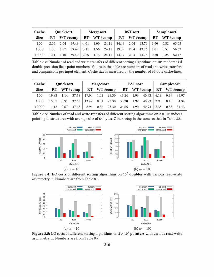
Cache Quicksort Mergesort BST sort Samplesort

Size RT WT #comp RT WT #comp RT WT #comp RT WT #comp

100 2.06 2.04 39.49 4.01 2.00 24.11 24.49 2.04 43.76 1.60 0.82 63.051000 1.58 1.57 39.49 3.11 1.56 24.11 19.39 2.04 43.76 1.01 0.51 56.6310000 1.11 1.10 39.49 2.25 1.13 24.11 14.17 2.03 43.76 0.50 0.25 52.47

Table 8.8: Number of read and write transfers of dierent sorting algorithms on 107 random i.i.d.double-precision oat-point numbers. Values in the table are numbers of read and write transfersand comparisons per input element. Cache size is measured by the number of 64-byte cache-lines.

Cache Quicksort Mergesort BST sort Samplesort

Size RT WT #comp RT WT #comp RT WT #comp RT WT #comp

100 19.83 1.14 37.68 17.04 1.02 23.30 46.24 1.93 40.93 6.19 0.79 35.971000 15.57 0.91 37.68 13.42 0.81 23.30 35.30 1.92 40.93 3.93 0.45 34.3410000 11.12 0.67 37.68 8.96 0.56 23.30 24.65 1.90 40.93 2.38 0.38 34.43

Table 8.9: Number of read and write transfers of dierent sorting algorithms on 2 × 106 indicespointing to structures with average size of 64 bytes. Other setup is the same as that in Table 8.8.

0

10

20

30

40

50

100 1000 10000

(Rel

ativ

e) I

/O c

ost

Cache Size

quicksortmergesort

BSTsortsamplesort

(a) ω = 10

0

50

100

150

200

250

300

100 1000 10000

(Rel

ativ

e) I

/O c

ost

Cache Size

quicksortmergesort

BSTsortsamplesort

(b) ω = 100Figure 8.4: I/O costs of dierent sorting algorithms on 107

doubles with various read-writeasymmetry ω. Numbers are from Table 8.8.

0 10 20 30 40 50 60 70 80

100 1000 10000

(Rel

ativ

e) I

/O c

ost

Cache Size

quicksortmergesort

BSTsortsamplesort

(a) ω = 10

0

50

100

150

200

250

100 1000 10000

(Rel

ativ

e) I

/O c

ost

Cache Size

quicksortmergesort

BSTsortsamplesort

(b) ω = 100Figure 8.5: I/O costs of dierent sorting algorithms on 2 × 106

pointers with various read-writeasymmetry ω. Numbers are from Table 8.9.

216

parameters of the hardware. BST sort thus will still be less ecient to sort small andxed-structure entries in future memories.

The experiment result of samplesort follows our analysis as well: each round ofsample sort approximately requires three sequential reads and one sequential write, andthe algorithm uses roughly dlogM/B(n/B)e rounds to reach the base case. Other costs(sampling and sorting pivots, transposing the osets, etc.) are negligible.

Based on our previous experience, after highly optimizing the performance in the se-quential setting, samplesort is slightly slower than quicksort (but much faster in multicoreparallelism) even though the I/O cost of samplesort is lower. We believe the reason tobe that, samplesort does not explicitly utilize L1 and L2 caches (the binary search, osettranspose, etc.) so most small-memory accesses are toward L3 cache. The memory accesspattern for quicksort, however, is mostly sequential scanning, which is highly optimized(like by prefetching) in the current architecture. Since the write costs will signicantlyincrease for future non-volatile main memory, we project that samplesort will be moreecient in this setting, since the I/O cost will very likely be the bottleneck of all thesesorting algorithms (similar to the existing multicore parallel setting).

Sorting larger entries. As shown previously, although BST sort requires only at mostrandom two writes per insertion, this cost is still signicant compared to other sortingalgorithms that have better spatial locality in memory access. However, when the size ofeach input entry becomes larger, each cache-line holds fewer entries and the number ofwrite transfers per entry increases.

We run the experiment with a xed number of inputs (107) and cache-lines (1000),and varies the size of each input entry from 8 bytes to 64 bytes. The results are shown inTable 8.10. Based on the analysis in Section 8.5.1, for quicksort, mergesort, and samplesort,the I/O cost is proportional to the entry size. However, BST sort is mostly not aected.The number of reads just marginally increases since the cache can hold less top-treelevels, and slightly more writes are required since the overall footprint of the search treeincreases as the growth of the entry size. From the results, we can see that when theentry size becomes at least 64 bytes, BST sort outperforms all other algorithms in theasymmetric setting.

Performance on sorting via pointers. In this experiment, we sort 2 million randomstrings that the characters are stored contiguously in the memory with an average size of64 bytes. The input also contains 2 million 8-byte pointers to the strings, and we onlysort the pointers.

The implementations of quicksort, mergesort, and BST sort are identical except thateach comparison requires two indirect addresses to locate the data eld. Samplesort, sinceit is cache-aware, requires two modications: rst, no oversampling for the pivots sincenow each pivot requires one or two cache-lines for its data; second, instead binary-search

217

Entry Quicksort Mergesort BSTsort Samplesort

Size RT WT RT WT RT WT RT WT

8 1.58 1.57 3.25 1.63 19.39 2.04 1.01 0.5116 3.26 3.17 7.00 3.50 21.11 2.29 2.09 1.0832 6.58 6.13 15.00 7.50 23.04 2.79 4.25 2.2464 13.18 11.58 32.00 16.00 25.35 3.79 8.91 4.87

Table 8.10: Numbers of read and write transfers of dierent sorting algorithms with various datasizes (bytes). The input size is 107 and the cache contains 1000 cache-lines.

the bucket of each element twice, we now store the bucket label after the rst search toavoid the second search (roughly double the writes while half the reads).

The numbers of read and write transfers are reported in Table 8.9 and visualized fortwo typical values of ω (10 and 100) in Figure 8.5. Writes of quicksort, mergesort, and BSTsort stay approximately the same as the previous experiment (the decrease in values isdue to fewer input elements). Reads are now increased by about log2(nB/M), the cost oflocating the data elds.

For each round in sample sort, each element now requires one random read, threesequential reads and two sequential writes (i.e., 1.375 read transfers and 0.25 write transfer).Also, one extra random read per element is in the base case to load the data into the cache.The algorithm requiresO(logM/B(n)) rounds to reach the base case, and in the experiment,this round number is approximately 3, 2 and 1 for three cache sizes. Finally, output needsto be moved back when reaching the base case in an odd number of rounds.

As what we understand, the wall-clock performance of samplesort when sortingpointers on current architecture is already faster than the other sorts. This is becausesamplesort requires fewer I/Os and comparisons, and all algorithms randomly access thememory so techniques like prefetching cannot help. This gap will be even enlarged infuture NVMs when the write costs being exaggerated.

8.5.3 Conclusions

Based on our implementations and experiments, the following conclusions and theprojection of the techniques for future non-volatile main-memories can be drawn.

Samplesort. Samplesort generally requires fewer I/Os than other sorting algorithms.On existing hardware, since samplesort does not explicitly optimize for L1/L2 cache,its sequential performance is slightly slower than quicksort. However, in the multicoreparallel setting, samplesort is always the fastest due to its eciency on I/O cost. Wepredict that samplesort will play a more signicant role with the future hardware even in

218

the sequential setting, because of the lower number of accessing to the large asymmetricmemory and the asymmetry of bandwidth and energy on the new memories.

Sorting indirect pointers. The advantage of samplesort will be enlarged when sortingvia pointers. This is because samplesort requires fewer rounds to nish, and thereforeit uses fewer reads, fewer writes, and fewer comparisons compared to other algorithms.This also matches the observation on the existing symmetric setting that samplesort ismore ecient on wall-clock performance.

BST sort. Although BST sort only requiring constant writes on large-memory per update,it is still inecient compared to other approaches when sorting integers or oat-pointnumbers because of its lacking on utilizing the cache-lines. However, when sorting entrieswith at least 64 bytes (i.e., a cache-line size), the I/O cost of BST sort outperforms the restthree algorithms.

8.6 Graph Traversal Algorithms

We now provide the full version of the graph-traversal algorithms in this paper.We discuss two of the most commonly-used graph-traversing algorithms: Breadth-rstsearch (BFS), and Dijkstra’s Algorithm. We show that with appropriate implementations,these algorithms can write much fewer to the main memory, comparing to the classicimplementations.

Throughout this section we assume the input graph G = (V , E) contains n = |V |vertices andm = |E | edges.

8.6.1 Breadth-First Search

Breadth-rst search (BFS) is an algorithm for graph traversing or searching. It startsat the source node, which is an arbitrary node of a graph, and explores the vertices withrespect to the distances (the number of hops) from the source node. BFS is commonly-usedin computing single-source shortest paths on unweighted graphs, as a subroutine forgraph radii estimation, eccentricity estimation and betweenness centrality, and as a basicbuilding block for other graph algorithms like graph connectivity, reachability, bridges,biconnected components, and strongly connected components. In this paper we focuson the most basic application: shortest paths on undirected graphs, and the techniquesdiscussed here can apply to many other applications.

8.6.1.1 The Classic Implementation

Given a graph G = (V , E) with n vertices andm edges, the classic implementation ofBFS keeps a queue with size n, and an array of boolean ags with size n indicating thateach vertex is visited or not during the search. This implementation requires at most 2writes for each vertex: one sequential write for adding it to the queue and one random

219

access for changing the ag of this vertex. Meanwhile, searches along an edge to analready visited vertex require no writes. The overall I/O cost of BFS Q(n,m) = O(ωn +m)(Chapter 5).

This bound is asymptotic optimal for arbitrary graphs, since the output of BFS, theshortest-path tree, has size O(n). However, a number applications (e.g., s-t shortest-pathor connectivity, graph radii estimation or eccentricity estimation) have output size O(1),which allow techniques utilizing the small-memory and reducing the number of writes.

8.6.1.2 BFS Implementation using Rotating Arrays

The rotating arrays are used in many algorithms to reduce the space requirement.For example, the diamond DAG computation in the longest common subsequence (LCS)problem only requires storing two consecutive columns (or rows) at any time during thedynamic programming process, since each DP value only depends on three other nearbyvertices in the diamond DAG. The algorithm maintains two arrays each with the size ofeither input string: one to hold the results in odd columns (rows) while the other for theeven ones. We call this structure the rotating arrays since the two arrays are rotating andholding computed and uncomputed values. They only require temporal (cache) space ofone dimension although the nodes in the entire DAG have two dimensions.

Here we observe that BFS on undirected graphs can apply a similar approach: insteadof keeping a queue and a global array of boolean ags with size n, we maintain separatequeues, each corresponding to a specic frontier (i.e., the set of vertices with the samedistance to the source). This is because, during the BFS on undirected graphs, the outgoingedges from the i-th frontier can only reach the vertices in either the (i − 1)-th frontier orthe (i + 1)-th frontier. Otherwise, assume an edge reaches a vertex in the j(< i − 1)-thfrontier, then the vertex in j-th frontier will visit this vertex in (j + 1)-th frontier. Asa result, when processing the i-th frontier, we only need to keep three frontiers withdistance i − 1, i and i + 1.

Since each frontier is separately kept and all vertices in one frontier have the samedistances, we no longer need to keep the relative orders of the elements within eachfrontier. We hence directly use an unordered set to maintain each frontier. Since onlythree frontiers are useful during the BFS process, we also only allocate and keep threeunordered sets and their roles rotate among the previous, the current and the next frontier.

The 2-level hash table introduced in Section 8.4.1.1 works perfectly well here since wehave no control of the frontier sizes, which can be either greater or smaller than previousones. For each frontier, we loop over all vertices in the set, and for each outgoing edge, ifthe other endpoint is not in either of the three unordered sets then it is added to the nextfrontier. Therefore, the operations to the sets include lookups and insertions. We do notexplicitly delete the sets. Instead, when the searching of one frontier is nished, the newnext frontier will reuse this space of the previous frontier.

220

8.6.1.3 Bidirectional Search

This previous implementation based on rotating arrays can greatly reduce the numberof write transfer when the frontier size is much smaller than the number of vertices,like grids, meshes, roadmaps, etc. For other graphs with larger frontier size and smallerdiameter (e.g., real-world networks that follow power law), I/O cost is not improvedsignicantly. However for these graphs, the average distance between every pair ofvertices is usually very small, and this is called the “small-world phenomenon” [277].

To utilize this property, we employ bidirectional breadth-rst search on computingthe s-t shortest path. Assuming the distance between this pair of query vertices is d , thenthe search from each direction will only visit the vertices within distance dd/2e. On thesepower-law graphs, the frontier size grows exponentially on the rst several steps untilmost of the vertices are reached. The number of vertices on the top-half levels in theshortest-path tree is therefore far less than n. This dierence however, is negligible ongraphs with bounded frontier size, since the distance between a random pair of vertices islarge expectedly, and the bidirectional search eventually reaches about the same amountof vertices unless d is much smaller than the graph diameter.

To implement bidirectional search eciently, we also use three rotating arrays for thesearch process. The extra detail here is that, the source, destination, and all intermediatevertices are put together in the same sets, and use one bit (the sign bit) to identify if thevertex is by the search from the source or from the destination. We only keep three insteadof six sets, which reduces the number of read transfers approximately by a half.

8.6.1.4 Experiment

In the experiment, we examine whether and how the new algorithms we just discussedimprove the I/O cost. We implement four versions of breadth-rst search: classic andbidirectional search with and without using rotating arrays. The experiment is run on 8graph instances with various cache size.

Graph instances. We use graphs of various types from the SNAP datasets [199] as theinput of the algorithms. The graphs include the road networks in Pennsylvania and Texas(real-world planar graphs), the web graphs of the University of Notre Dame and StanfordUniversity, the DBLP collaboration network, and the Youtube online social network (4real-world networks). In the case of web graphs, each edge represents a hyperlink betweentwo web pages. We also use synthetic graphs of 2D and 3D grids. For each of the graphsused, the numbers of vertices and edges are given in the table below. If a graph does notcome equipped with weights, we assign to every edge a random integer between 1 and10, 000. The graphs we used are relatively small due to the overhead in our software andhardware simulator, but we adjust the cache size accordingly.

Overall performance. The numbers of read and write transfers on 8 graph instanceswith various cache size are given in Table 8.11. Their weighted I/O costs are given in

221

Type Graph # Vertices # EdgesGrid: 2D 1M 3.96M

Sparse Grid: 3D 1M 5.94MGraphs Roadmap: Pennsylvania 1.09M 3.08M

Roadmap: Texas 1.39M 3.84MWebgraph: Notre Dame 325K 2.20M

Social Webgraph: Stanford 281K 3.98MNetworks DBLP collab. network 317K 2.10M

Youtube network 1.13M 5.98M

Table 8.12 considering two typical values ofω, and visualized (merged into two categories)in Figure 8.6.

To better understand the performance of dierent implementations, we also countvarious statistics of the searching including the depths and frontier sizes, and the resultsare generalized in Table 8.13.

Unidirectional search. Indicated in Table 8.11, classic BFS requires no more than onesequential write (pushed into the queue) and one random write (marking the distance)per vertex. The random write can be avoided if the associated cache line is cached, sobetter locality of vertex indices of some graphs (roadmaps and NDU webgraph) and largercache size reduce writes per vertex. The algorithm also reads the edges of each vertex andchecks whether the other endpoint is visited or not, which is also aected by the edgesper vertex and the locality of vertex indices.

For the implementation using rotating arrays, the key factor is whether the frontierts into the cache. Shown in Table 8.13, the sparse graphs (grids and roadmaps) havesmaller frontier sizes, so as long as the cache can hold each of them, the writes are largelyminimized. This is also true for reads since checking is always in the hash table. However,once the frontier is larger than the cache size, then each insertion to the hash table nowbecomes a random write and can hardly be cached because of the hash function. Thereads are increased even more, since checking whether a vertex is visited can lead to atmost 6 cache misses: three rotating arrays each with 2 levels. Summarized in Figure 8.6,the I/O cost is largely improved using the rotating arrays when frontiers t into the cache,but deteriorates when not.

Bidirectional search. The I/O performance of classic bidirectional BFS is similar tothe classic unidirectional BFS since they essentially search in a similar pattern. Thebidirectional search requires fewer reads and writes since it strictly searches fewer vertices,especially in social networks since these graphs have smaller diameters and the twosearches usually meet earlier before the majority of the vertices are visited.

222

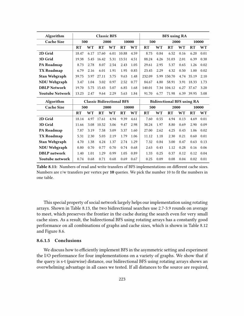
Algorithm Classic BFS BFS using RA

Cache Size 500 2000 10000 500 2000 10000

RT WT RT WT RT WT RT WT RT WT RT WT

2D Grid 18.47 6.17 17.60 6.01 10.88 4.59 8.75 0.84 6.52 0.16 6.20 0.013D Grid 19.38 5.45 16.42 5.31 13.51 4.51 88.24 4.26 31.03 2.01 6.39 0.38PA Roadmap 8.73 2.78 8.07 2.54 2.43 1.05 29.61 2.95 5.37 0.65 1.26 0.02TX Roadmap 6.79 2.16 6.01 1.91 1.95 0.85 23.45 2.29 4.32 0.50 1.00 0.02Stan Webgraph 39.75 3.97 27.11 3.75 9.63 1.48 232.09 5.99 150.70 4.74 35.19 2.10NDUWebgraph 3.47 1.04 3.02 0.97 2.52 0.77 84.67 4.80 58.91 3.91 18.33 1.73DBLP Network 19.70 5.75 15.43 5.07 6.85 1.68 140.01 7.34 104.12 6.27 37.67 3.20Youtube Network 13.23 2.47 9.64 2.29 5.63 1.84 91.70 6.77 71.98 6.39 39.95 5.08

Algorithm Classic Bidirectional BFS Bidirectional BFS using RA

Cache Size 500 2000 10000 500 2000 10000

RT WT RT WT RT WT RT WT RT WT RT WT

2D Grid 18.14 4.97 17.61 4.94 9.39 4.61 7.60 0.55 4.94 0.13 4.69 0.013D Grid 11.66 3.08 10.52 3.06 9.47 2.98 38.24 1.97 8.80 0.69 2.90 0.09PA Roadmap 7.87 3.19 7.58 3.09 3.37 1.60 27.00 2.62 4.25 0.43 1.06 0.02TX Roadmap 5.31 2.30 5.03 2.19 1.79 1.06 11.12 1.18 2.30 0.21 0.60 0.01Stan Webgraph 4.70 1.38 4.24 1.37 2.74 1.29 7.32 0.84 3.00 0.47 0.63 0.13NDUWebgraph 0.80 0.70 0.77 0.70 0.74 0.68 2.63 0.43 1.12 0.28 0.16 0.06DBLP network 1.40 1.01 1.29 0.99 1.05 0.89 1.33 0.25 0.37 0.12 0.12 0.04Youtube network 0.74 0.68 0.71 0.68 0.69 0.67 0.25 0.09 0.08 0.04 0.02 0.01

Table 8.11: Numbers of read and write transfers of BFS implementations on dierent cache sizes.Numbers are r/w transfers per vertex per 10 queries. We pick the number 10 to t the numbers inone table.

This special property of social network largely helps our implementation using rotatingarrays. Shown in Table 8.13, the two bidirectional searches use 2.7-3.9 rounds on averageto meet, which preserves the frontier in the cache during the search even for very smallcache sizes. As a result, the bidirectional BFS using rotating arrays has a constantly goodperformance on all combinations of graphs and cache sizes, which is shown in Table 8.12and Figure 8.6.

8.6.1.5 Conclusions

We discuss how to eciently implement BFS in the asymmetric setting and experimentthe I/O performance for four implementations on a variety of graphs. We show that ifthe query is s-t (pairwise) distance, our bidirectional BFS using rotating arrays shows anoverwhelming advantage in all cases we tested. If all distances to the source are required,

223

ω = 10Algorithm Classic BFS BFS using RA Classic Bidir. BFS Bidir. BFS using RA

Cache Size 500 2000 10000 500 2000 10000 500 2000 10000 500 2000 10000

2D Grid 80.18 77.72 56.74 17.13 8.15 6.25 67.80 67.04 55.53 13.14 6.27 4.763D Grid 73.85 69.49 58.60 130.86 51.16 10.18 42.44 41.16 39.29 57.98 15.65 3.82PA Roadmap 36.50 33.42 12.89 59.10 11.84 1.44 39.76 38.46 19.39 53.24 8.52 1.24TX Roadmap 28.42 25.14 10.44 46.36 9.36 1.18 28.27 26.95 12.37 22.89 4.37 0.69Stan Webgraph 79.41 64.64 24.39 291.99 198.08 56.18 18.48 17.93 15.62 15.75 7.71 1.93NDUWebgraph 13.84 12.70 10.20 132.71 98.04 35.58 7.80 7.73 7.54 6.90 3.90 0.75DBLP network 77.19 66.16 23.67 213.43 166.84 69.63 11.53 11.22 9.91 3.84 1.61 0.56Youtube network 37.92 32.59 24.06 159.43 135.92 90.72 7.58 7.50 7.38 1.17 0.51 0.17

ω = 100Algorithm Classic BFS BFS using RA Classic Bidir. BFS Bidir. BFS using RA

Cache Size 500 2000 10000 500 2000 10000 500 2000 10000 500 2000 10000

2D Grid 635.5 618.7 469.4 92.5 22.7 6.7 514.7 511.8 470.7 62.9 18.2 5.33D Grid 564.0 547.1 464.3 514.4 232.3 44.2 319.4 316.9 307.6 235.6 77.4 12.0PA Roadmap 286.4 261.5 107.0 324.4 70.0 3.0 326.7 316.4 163.6 289.4 47.0 2.8TX Roadmap 223.1 197.3 86.8 252.5 54.7 2.8 234.8 224.2 107.6 128.8 23.0 1.5Stan Webgraph 436.3 402.4 157.1 831.1 624.5 245.1 142.5 141.2 131.6 91.6 50.1 13.6NDUWebgraph 107.1 99.8 79.2 565.0 450.2 190.8 70.8 70.3 68.8 45.3 28.9 6.0DBLP network 594.6 522.6 175.1 874.2 731.3 357.3 102.6 100.5 89.7 26.4 12.8 4.5Youtube network 260.2 239.1 190.0 769.0 711.4 547.6 69.1 68.5 67.6 9.4 4.3 1.5

Table 8.12: I/O costs of BFS implementations on dierent cache sizes. Numbers of r/w transfersare from Table 8.11. Italic-font number indicates that the classic implementation has a lower I/Ocost in that setting.

the unidirectional BFS using rotating arrays has a better performance if the cache canhold each frontier.

8.6.2 Dijkstra’s Algorithm

Dijkstra’s Algorithm [114] is a well-known algorithm to compute single-source short-est paths on a non-negative weighted graph G = (V , E). Due to the rapid growth ofthe data size, real-world graphs nowadays can easily go beyond the size of the order ofgigabytes, and they need to be stored on the large non-volatile memory. Running theclassic implementation of Dijkstra’s algorithm can be costly in this setting. We showthat with an appropriate implementation, the algorithm can write much fewer to thenon-volatile memory, which further leads to much lower I/O cost.

224

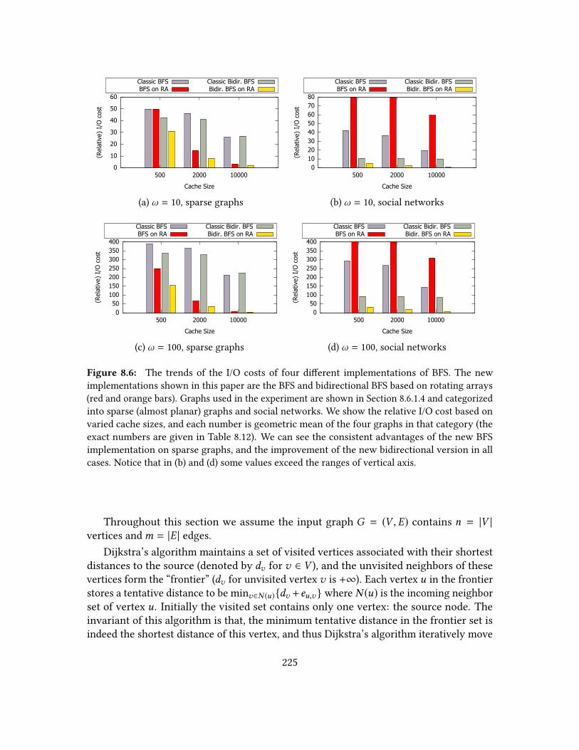
0

10

20

30

40

50

60

500 2000 10000

(Rel

ativ

e) I

/O c

ost

Cache Size

Classic BFSBFS on RA

Classic Bidir. BFSBidir. BFS on RA

(a) ω = 10, sparse graphs

0 10 20 30 40 50 60 70 80

500 2000 10000

(Rel

ativ

e) I

/O c

ost

Cache Size

Classic BFSBFS on RA

Classic Bidir. BFSBidir. BFS on RA

(b) ω = 10, social networks

0 50

100 150 200 250 300 350 400

500 2000 10000

(Rel

ativ

e) I

/O c

ost

Cache Size

Classic BFSBFS on RA

Classic Bidir. BFSBidir. BFS on RA

(c) ω = 100, sparse graphs

0 50

100 150 200 250 300 350 400

500 2000 10000

(Rel

ativ

e) I

/O c

ost

Cache Size

Classic BFSBFS on RA

Classic Bidir. BFSBidir. BFS on RA

(d) ω = 100, social networks

Figure 8.6: The trends of the I/O costs of four dierent implementations of BFS. The newimplementations shown in this paper are the BFS and bidirectional BFS based on rotating arrays(red and orange bars). Graphs used in the experiment are shown in Section 8.6.1.4 and categorizedinto sparse (almost planar) graphs and social networks. We show the relative I/O cost based onvaried cache sizes, and each number is geometric mean of the four graphs in that category (theexact numbers are given in Table 8.12). We can see the consistent advantages of the new BFSimplementation on sparse graphs, and the improvement of the new bidirectional version in allcases. Notice that in (b) and (d) some values exceed the ranges of vertical axis.

Throughout this section we assume the input graph G = (V , E) contains n = |V |vertices andm = |E | edges.

Dijkstra’s algorithm maintains a set of visited vertices associated with their shortestdistances to the source (denoted by dv for v ∈ V ), and the unvisited neighbors of thesevertices form the “frontier” (dv for unvisited vertex v is +∞). Each vertex u in the frontierstores a tentative distance to be minv∈N (u)dv +eu,v where N (u) is the incoming neighborset of vertex u. Initially the visited set contains only one vertex: the source node. Theinvariant of this algorithm is that, the minimum tentative distance in the frontier set isindeed the shortest distance of this vertex, and thus Dijkstra’s algorithm iteratively move

225

Unidirectional search Bidirectional search

depth maximum

frontier

size

average

frontier

size

depth maximum

frontier

size

average

frontier

size

2D Grid 1571.4 1460 636.4 370.2 2091 1102.83D Grid 229.9 13277 4349.7 49.3 15058 4628.9PA Roadmap 574.5 5032 1893.1 163.9 7204 2718.3TX Roadmap 748.6 6058 1804.9 174.7 5752 2102.1Stan Webgraph 107.1 87614 2383.4 3.5 50094 3782.8NDUWebgraph 29.2 124519 11155.1 3.8 51562 2053.5DBLP Network 16.1 129283 19694.4 3.9 36373 1420.1Youtube Network 15.8 607534 71828.5 2.7 1841 107.4

Table 8.13: The depths (number of levels in the shortest-path tree) and frontier sizes (number ofvertices) during the search processes. Note that the numbers are averaged from multiple searches.

this vertex from the frontier to the visited set and update the frontier accordingly. Thecorrectness can easily be proven by induction on the number of visited nodes.

Due to the widespread use of Dijkstra’s algorithm, there are plenty of works onthe ecient implementations of Dijkstra’s algorithm and we refer the readers to somerecent works [69, 213] for summaries of the work bounds of dierent approaches. Dier-ent implementations have dierent costs on the two operations in Dijkstra’s algorithm:Extract-Min that nds and removes the vertex with minimum distance in the frontierset, and Decrease-Key that updates the tentative distance of the other endpoint of anedge of this vertex removed from the frontier in this iteration. The data type that supportsthe queries is abstracted as a priority queue. Specically when the priority queue isimplemented using Fibonacci Heap [128] to maintain the frontier set, the overall timecomplexity is O(m + n logn).

8.6.2.1 Classic Implementation using a Binary Heap

Although there are many advanced implementations of the priority queue with lowertime complexities, the constant hidden in the asymptotic bound is large. In practicethe classic implementation using a binary heap works reasonably well on general sparsereal-world graphs, and its wall-clock performance is competitive or even better on moderncomputer architecture. We hence implement it as a baseline and measure the number ofread and write transfers of this algorithm as a comparison to our write-ecient version.

For each vertex, we maintain the shortest distance in a global array with size n.For practical purpose, instead of initializing the priority queue of size n with innite

226

distances, we insert a vertex when it is rst added to the frontier (so the priority queueneeds to support Insert, which most implementations do). The binary heap only storesthe indices of the vertices which optimizes the memory footprint and number of writetransfers. To perform Decrease-Key in a binary heap eciently, we keep another globalarray, an auxiliary structure that maps each vertex to its position in the heap, and ismaintained up-to-date as the priority queue changes. This implementation has worst-casetime complexity to be O(m logn). Since this implementation does not take any specialoptimization on caching, the I/O cost is therefore O(ωm log(nB/M)), assuming the cachealways keeps the rst M/B vertices in the priority queue.

8.6.2.2 Phased Dijkstra

Phased Dijkstra (Section 5.4.1) is a specic implementation of Dijkstra’s algorithmthat the goal is to fully maintain the priority queue in small-memory. It only requiresO(n) writes to large-memory, the shortest distances to all vertices. The idea is to partitionthe computation into phases such that for a parameter M′ each phase keeps a priorityqueue of size at most (1 + ϵ)M′ and visits at least M′ vertices. By selecting M′ = M/c foran appropriate constant c , the priority queue ts in small-memory, and the only writes tolarge-memory are the nal distances.

Algorithm 15: Phased DijkstraInput: A connected weighted graph G = (V , E) and a source vertex sOutput: The shortest distances δ = δ1, . . . , δn from source s

1 Priority Queue P ← 2 Mark vertex s as visited and set δ (s) ← 03 while there exists unvisited vertices do4 if P = then

5 Scan over all edges in E and store at most M ′ closest unvisited vertices in P6 if |P | = M ′ then7 Set dmax as the distance to the farthest vertex in P8 else

9 dmax ← +∞10 u = P .Extract-Min()11 Set δu as the distance from s to u, and mark u as visited12 foreach (u,v, disu ,v ) ∈ E do

13 if δu + disu ,v < dmax then

14 if v ∈ P then

15 P .Decrease-Key(v, δu + disu ,v )16 else

17 P .insert(v, δu + disu ,v )18 if |P | = (1 + ϵ)M ′ then19 Remove ϵM ′ vertices with larger distances in P20 Set dmax as the farthest distance in P21 return δ (·)

The pseudocode of the algorithm is provided in Algorithm 15. Technically the priorityqueue P can be implemented using an arbitrary heap since it is fully in the small-memoryand will not aect the I/O cost. In our experiment we implement it using a binary heap.

227

In phased Dijkstra, each phase starts and ends with an empty priority queue P . Thepriority queue is kept small by discarding the ϵM′ largest elements (vertex distances)whenever |P | = (1 + ϵ)M′. To achieve this, P is attened into an array, the M′-th smallestelement dmax is found by selection, and the priority queue is reconstructed from theelements no greater than dmax , all taking linear time. After such a truncation, all furtherinsertions in a given phase are not added to P if they have a value greater than dmax .

The processing of each phase in phased Dijkstra consists of two parts. The rstpart (line 5–9) of each phase loops over all edges in the graph and relaxes any that gofrom a visited to an unvisited vertex (possibly inserting or decreasing a key in P ). Thesecond part (repeatedly loop over line 10–20) then runs standard Dijkstra’s algorithmrepeatedly visiting the vertex with minimum distance and relaxing its neighbors until Pis empty. Similar to other implementations, to implement relax, the algorithm needs toknow whether a vertex is already in P , and if so where in P so that it can do a decrease-keyon it. However in phased Dijkstra it is too costly to store this information using a globalarray. Instead, we use an unordered map introduced in Section 8.4.1.1 for this mapping.Theoretically the hash table can be set with xed size, but in practice we use a 2-levelhash table since it leads to better performance when the frontier size is consistently small,and equal performance otherwise. This map is referred as vertex map later.

The I/O cost of phased Dijkstra is Q(n,m) = O(n(mM+ ω

)). More details on the

correctness and complexity analysis can be found in Section 5.4.1.We make a special optimization that once all outgoing edges of a vertex are visited,

we remove this node and all associated edges in the scan in Line 5. This is done by usingthe sign-bit of the output distances, such that it is more likely being cached. We call theactive set that contains visited but not removed vertices.

For an ecient implementation that optimizes memory footprint and I/O eciency,each heap element contains the vertex index, the pointer to the vertex map, and thetentative distance. In total it takes 16 bytes. Each element in the vertex map only stores apointer, and the vertex index can be check via the corresponding heap element. Through-out our experiment we set the maximum occupancy rate of the 2-level hash table to be 0.8,and truncation ratio ϵ = 0.25. M′ is chosen such that the hash table and priority queueoccupy about 40% of the small-memory, while various values of M′ are also discussed.

8.6.2.3 Experiments

The experiments are run on two Dijkstra implementations with dierent parametercombinations on cache size, cache policy, and the priority queue size. The experiment isrun on eight graph instances with various cache size.

Since in phased Dijkstra the number of reads is signicantly more than that of writes,to keep the priority queue in the cache, the special cache strategy in Section 8.3.2 is

228

Classic Dijkstra using binary heap Phased Dijkstra

Cache Size 2k 10k 50k 2k 10k 50k

Graph Instance RT WT RT WT RT WT RT WT RT WT RT WT

2D Grid 10.37 4.87 4.61 2.34 3.53 1.89 5.93 1.12 (1) 3.62 1.11 (1) 2.74 1.04 (1)3D Grid 25.87 14.53 17.44 8.54 8.20 3.35 126.56 1.12 (383) 28.16 1.12 (44) 5.90 1.07 (1)PA Roadmap 7.82 4.14 2.16 0.81 1.12 0.40 30.40 0.99 (202) 1.89 0.52 (1) 1.04 0.28 (1)TX Roadmap 7.69 4.10 2.16 0.82 1.09 0.40 37.93 0.97 (262) 1.88 0.53 (1) 1.01 0.27 (1)Stan Webgraph 37.31 18.13 26.73 12.06 10.60 3.91 404.61 1.03 (100) 81.02 1.02 (16) 13.83 0.88 (2)NDUWebgraph 24.97 15.34 15.14 8.21 5.19 1.65 99.86 1.10 (132) 22.57 1.01 (24) 5.81 0.67 (3)DBLP Network 32.14 19.66 23.17 13.02 10.08 4.58 341.08 1.12 (131) 64.75 1.10 (24) 11.53 0.94 (4)Youtube Network 35.19 22.86 26.80 16.53 21.18 12.90 836.64 1.13 (477) 161.36 1.11 (93) 33.08 1.05 (18)

Table 8.14: Number of read and write transfers of dierent Dijkstra implementations on dierentcache size. Numbers are normalized to read or write transfers per vertex. We ran SSSP queries on10 dierent randomly-chosen source nodes. Numbers in the parentheses are the average phases.

ω = 10 ω = 100Classic Phased Dijkstra Classic Phased Dijkstra

Cache Size 2k 10k 50k 2k 10k 50k 2k 10k 50k 2k 10k 50k

2D Grid 59.1 28.0 22.4 17.1 14.7 13.1 497.8 238.9 192.2 118.3 114.3 106.83D Grid 171.2 102.8 41.7 137.8 39.3 16.6 1478.9 871.2 343.5 239.0 140.1 113.1PA Roadmap 49.2 10.2 5.1 40.3 7.1 3.8 421.4 83.1 41.2 129.0 53.9 28.7TX Roadmap 48.7 10.4 5.1 47.6 7.1 3.7 417.5 84.3 40.9 134.5 54.5 28.3Stan Webgraph 218.6 147.3 49.7 414.9 91.2 22.6 1850.2 1232.2 401.8 507.7 182.8 101.9NDUWebgraph 178.4 97.2 21.6 110.9 32.7 12.5 1559.4 836.3 169.7 209.9 123.9 72.8DBLP Network 228.7 153.4 55.9 352.3 75.7 20.9 1997.6 1325.2 468.4 453.1 174.7 105.9Youtube Network 263.8 192.1 150.1 847.9 172.5 43.6 2321.0 1679.4 1310.8 949.3 272.8 138.3

Table 8.15: The I/O costs on dierent Dijkstra implementations on dierent cache size. Thewrite-read ratio ω are selected to be typical projected values 10 (latency, bandwidth) and 100(energy). Results are based on the numbers in Table 8.14.

required. In Table 8.16 we show that dierent cache policies only cause minor dierences,so in the majority of this section we use the Static policy.

Overall performance. In Table 8.14 we show the number of read and write transfers oftwo implementations on dierent graphs with various cache size. Cache size varies from2,000 to 50,000 cache lines each with 64 bytes. In Table 8.15 the overall I/O costs withdierent values of ω are listed based on the numbers in Table 8.14.

For the binary-heap implementation, the actual reads and writes mostly match thetheoretical bound O(m log(nB/M)). Reads are about slightly less than twice as writes:each edge is read once during Dijkstra (linear scan and requires no modication), and an

229

0 10 20 30 40 50 60 70 80

100 1000 10000

(Rel

ativ

e) I

/O c

ost

Cache Size

ClassicPhased Dijkstra

(a) ω = 10, sparse graphs

0 50

100 150 200 250 300 350 400

100 1000 10000

(Rel

ativ

e) I

/O c

ost

Cache Size

ClassicPhased Dijkstra

(b) ω = 10, social networks

0

100

200

300

400

500

600

700

100 1000 10000

(Rel

ativ

e) I

/O c

ost

Cache Size

ClassicPhased Dijkstra

(c) ω = 100, sparse graphs

0

500

1000

1500

2000

100 1000 10000

(Rel

ativ

e) I

/O c

ost

Cache Size

ClassicPhased Dijkstra

(d) ω = 100, social networks

Figure 8.7: I/O costs of classic Dijkstra and phased Dijkstra. Graphs are categorized into sparse(almost planar) graphs and social networks and the I/O cost is geometric mean of the four. Numbersare from Table 8.15.

update in the binary heap always requires one more read than writes. The only exceptionis on the roadmaps when the frontier size is consistently small while nearby vertices sharecontiguous indices. In this case the cache eciently holds the entire heap and leads tofewer reads and writes to the large-memory.

For phased Dijkstra, we rst observed that the number of writes is always no morethan 1.3 per vertex: one write per vertex when the distance is nalized, plus some othercost to maintain the active set. The number of read transfers is mainly decided the numberof phases, and the size of the active set (the edge lists of active vertices at the beginningof each phase needs to be scanned).

The overall I/O performance (shown in Table 8.15) indicates that phased Dijkstra isconsistently better than the binary-heap version except for the only case that both ω andcache size are small and the active set is large. This case can hardly happen in practice

230

since the cache size is even much smaller than the current L3 cache. The improvementon I/O cost in all cases is up to 3 and 7.6 when ω is 10 and 100. This peak occurs whenthe small-memory sizes is large and frontier size is larger, since at this time the cost tomaintain the binary heap in the classic implementation is costly, while the extra cost torun phased Dijkstra is insignicant.

Cache Policy SplitPool Static

RT WT RT WT

2D Grid 3.74 1.11 3.62 1.113D Grid 27.43 1.12 28.16 1.12PA Roadmap 1.84 0.88 1.89 0.52TX Roadmap 1.83 0.87 1.88 0.53Stan Webgraph 81.40 1.02 81.02 1.02NDUWebgraph 21.96 1.07 22.57 1.01DBLP Network 65.20 1.11 64.75 1.10Youtube Network 163.38 1.12 161.36 1.11

Table 8.16: Number of read and write transfer of phased Dijkstra with two dierent cache policies:the SplitPool policy and the Static policy. The cache contains 10,000 cache-lines. Dierent policiesgive very similar performance except for the writes on roadmaps.

Priority Queue Size 30% 40% 50% 60%

RT WT RT WT RT WT RT WT

2D Grid 8.4 1.10 8.6 1.11 8.9 1.11 9.3 1.113D Grid 33.7 1.12 28.9 1.12 25.6 1.12 23.3 1.12PA Roadmap 2.7 0.48 2.8 0.52 3.0 0.58 3.2 0.66TX Roadmap 2.6 0.48 2.7 0.53 2.9 0.59 3.1 0.66Stan Webgraph 94.4 1.02 82.9 1.02 72.1 1.02 67.1 1.02NDUWebgraph 26.1 1.01 22.8 1.01 20.2 1.03 18.5 1.04DBLP Network 75.1 1.10 64.9 1.10 57.3 1.10 51.5 1.11Youtube Network 183.8 1.11 161.5 1.11 144.4 1.12 134.9 1.12

Table 8.17: Number of read and write transfers of phased Dijkstra with dierent priority queue’ssize. The overall percentage of priority queue and vertex map varies from 30% to 60% comparingto the cache size, which is 10,000 cache-lines.

Dierent cache maintenance policy. We show the number of read and write transferof phased Dijkstra on two dierent cache policies in 8.16. Dierent policies actually give

231

a very similar performance in the graph instances. More analysis is shown in the fullversion of this paper.

Picking appropriate priority queue’s sizeM′. In previous experiment we empiricallyset the overall size of the priority queue and vertex map to be about 40% of the overallcache size. However, this percentage can aect the performance of phased Dijkstra. Largerpercentage leads the heap to contain more elements so that the overall number of phases isdecreased. Meanwhile the size left for the rest cache is smaller, which decreases the cacheperformance. Hence, the number of phases and specic graph property lead to dierentoptimality point of the the priority queue’s size and no easy conclusions can be drawn. InTable 8.17 we show a snapshot on the cache size of 10,000 and the percentage varies from30% to 60%. The trend is that, when the priority queue’s size is smaller than the averagefrontier size then larger priority queue helps, and vice visa. In general dierent priorityqueue’s sizes only make a minor dierence on I/O cost and will not aect the relativelylower cost comparing to the binary-heap implementation.

8.6.2.4 Conclusions

We discussed phased Dijkstra and experiment its performance on a variety of graphs.The high-level idea is to t the computation within the small-memory (i.e., the cache) andthus requires no intermediate writes to the large asymmetry memory. The experimentalresults show that phased Dijkstra consistently outperforms the binary-heap version onI/O cost except for the combination of small ω (= 10), small cache size, and on socialnetworks. Although phased Dijkstra contains some parameters, we also show that theydo not aect the eciency of phased Dijkstra when they are within a reasonable largerange. A similar case also holds for dierent cache policies.

Notice that the idea here that ts the computation in the small-memory can also beapplied to computing minimum spanning tree, sorting, and many other problems.

232

Chapter 9

Conclusion and Future Work

9.1 Conclusion

This thesis provides a comprehensive study of write-ecient algorithms, from com-putational models, to lower and upper bounds, experiments, as well as guaranteeing thefault-tolerance of the write-ecient algorithms. These write-ecient algorithms willhave improved performance on the new non-volatile main memory with asymmetric readand write costs, or can provide additional functionality with little costs in other recentsettings that may lead to write-read asymmetry.

This thesis discusses how to extend the most commonly-used computational modelsand cost measures used in analyzing classic algorithms to the asymmetric setting inChapter 2, which provides the theoretical approaches to analyze the algorithms asymptot-ically. Based on the models, researches can analyze lower bounds of the problems in theasymmetric setting, and a list of known results are shown in Chapter 3 and 7.

The main contribution of this thesis consists of a list of new write-ecient algorithms.They are widely spread from the basic algorithmic building blocks (sorting, reduce, lter,etc.) in Chapter 4, to graph algorithms (e.g., (bi)connectivity, shortest paths, MST, BFS)in Chapter 5, geometric algorithms and data structures (e.g., convex hull, Delaunaytriangulation, k-d trees, augmented trees) in Chpater 6, as well as many cache-obliviousalgorithms for dynamic programming and linear algebra problems 7. All these algorithmshave asymptotically improved cost under the sequential (M,ω)-ARAM or the parallelAsymmetric NP model. Also, most of these algorithms are highly parallelized. Since thenew memories provide a much larger (terabyte-level) capacity, parallelism is a necessityto process data with such volume.

It is interesting to point out that, this thesis also introduces many new techniques andanalysis frameworks on many types of algorithms. Each of them not only leads to manynew write-ecient algorithms, but also is of independent interests since many results inthe symmetric settings on these problems can also be improved based on it.

233

This thesis also contains experiment verications of the write-ecient algorithms inChapter 8. This part contains the rst experimental framework to analyze the performanceof write-ecient algorithms in practice, and experiments on a variety of algorithms whichleads to many interesting ndings and lessons.

9.2 Future Work

This thesis consolidates the research of write-ecient algorithms, which is a relativelynew research topic. It is notable that this is still a very open area, and there are many newproblems worth to be investigated. A few of the interesting future topics are listed here.

Actual Performance.

The new hardware has been manufactured at the time when this thesis is being written.As a result, it is reasonable to assume that the new hardware will be available to the publicvery soon. When it becomes available, implementing the write-ecient algorithms andtesting their actual wall-clock performance is denitely one of the works that shouldbe investigated. As discussed in Chapter 8, the software simulator for write-ecientalgorithms is still a useful tool even when the hardware is available. However, it isinteresting to know the best parameter to set in the simulator that can t the performancein practice the best. Also, it is of notable importance to have the highly-optimizedimplementations to be in an available library, so researchers or other programmers whosework is not performance engineering can directly call the functions in the library.

Write-ecient algorithms.

This thesis discusses a few dozens of new write-ecient algorithms, but this is still arelatively small amount compared to the entity of the algorithms that are widely beingused in practice. The write-ecient versions of these algorithms remain to be a futureresearch topic.

Other than designing write-ecient algorithms for other problems, the new problemsraised by studying the write-ecient algorithms in this thesis can also lead to potentialfuture work. For example, many new problems are proposed by the analysis framework ofthe k-d grid computation structure in Section 7.9. There are many unanswered questionsfor geometric algorithms as well.

This thesis discusses the implicit k-decomposition and the compact representations forconnectivity and biconnectivity information of a graph. It is interesting to know whethersuch kinds of compact representations of other graph problems, or even data structureand other problems (like a triangulation). A further question is the tradeo between thespace requirement, the number of writes, and the total algorithmic instructions for eachproblem. It remains unknown if one can show the lower bounds of a combination of theseterms for graph connectivity, and we can ask similar questions to other graph problemsas well.

234

Persistency and fault-tolerance.

As discussed in Section 1.1.2, another major property of these new main memories aretheir non-volatility or persistency: unlike DRAM, they have the capability of survivingpower outages and other failures without losing data. As a result, it is possible to designthe special programming model and algorithms that are resilient to either the processorfault or the power lost.

The consistent states of the intermediate data stored in the persistent main memoryneed to be guaranteed such that either a single processor or the entire program can berestarted from here. On the other hand, standard caches are write-back (write-behind),meaning that a write to a memory location will make it as far as the cache, until at somelater point the updated cache line gets ushed out to the persistent memory. Usuallythe programmers have no control of this process. Therefore, a fault-tolerant algorithmrunning on the persistent main memory needs to explicitly ush some of the cache lines toguarantee the desired states of the data in the persistent memory, using instructions (suchas Intel’s CLFLUSH instruction) supported by various programming models (e.g., [178, 240,241]). Such instructions require memory barriers to enforce the ordering in the execution,which leads to extra cost for these writes such as in synchronizing the processors. As aresult, the new non-volatile main memory provides the option for algorithms to programsto be fault resilient, but maintaining the memory consistency can cause the costly writeson these memories to be even more expensive. Write-ecient algorithms can be ecientin such settings because of the fewer overall writes that need to be ushed to the persistentmain memory.

However, as a rst step, we need to rst have a programming model to support suchfault-tolerant programming. Such a model is introduced by Belleoch et al. [71], whichis named as the Parallel Persistent Memory (Parallel-PM) model. Based on this model, wecan discuss how to make algorithms to be fault-tolerant, with or without considering themore expensive writes.

The Parallel Persistent Memory (Parallel-PM) model, consists of P processors, eachwith a fast local ephemeral memory of limited size M , and sharing a large slower persistentmemory. As in the external memory model [29, 30], each processor runs a standardinstruction set from its ephemeral memory and has instructions for transferring blocks ofsize B to and from the persistent memory. The cost of an algorithm is calculated based onthe number of such transfers, and the cost can be either symmetric or asymmetric. A keydierence, however, is that the model allows for individual processors to fault at any time.If a processor faults, all of its processor state and local ephemeral memory is lost, but thepersistent memory remains. We consider both the case where the processor restarts (softfaults) and the case where it never restarts (hard faults).

The model is motivated by two complimentary trends. Firstly, it is motivated byupcoming non-volatile memories that are nearly as fast as existing random access memory(DRAM), are accessed via loads and stores at the granularity of cache lines, and have large

235

capacity (more bits per unit area than existing random access memory). For example,Intel’s 3D-Xpoint memory technology, currently available as an SSD, is scheduled to beavailable as such a random access memory in 2019. While such memories are expectedto be the pervasive type of memory [210, 221, 283], each processor will still have a smallamount of cache and other fast memory implemented with traditional volatile memorytechnologies (SRAM or DRAM). Secondly, it is motivated by the fact that in current andupcoming large parallel systems the probability that an individual processor faults is notnegligible, requiring some form of fault tolerance [83].

In this model, a single processor version, the PM model, is rst discussed, which givesconditions under which programs are robust against faults. In particular, we identify thatbreaking a computation into “capsules” that have no write-after-read conicts (writing alocation that was read earlier within the same capsule) is sucient, when combined withour approach to restarting faulting capsules from their beginning, due to its idempotentbehavior. We then show that RAM algorithms, external memory algorithms, and cache-oblivious algorithms [131] can all be implemented asymptotically eciently on the model.This involves a simulation that breaks the computations into capsules and buers writes,which are handled in the next capsule. However, the simulation is likely not practical.We therefore consider a programming methodology in which the algorithm designercan identify capsule boundaries, and ensure that the capsules are free of write-after-readconicts.

Then the multiprocessor counterpart, the Parallel-PM described above, is considered,which gives conditions under which programs are correct when the processors are inter-acting through the shared memory. We identify that if capsules are free of write-after-readconicts and atomic, in a way that we dene, then each capsule acts as if it ran oncedespite many possible restarts. Furthermore we identify that a compare-and-swap (CAS)instruction is not safe in the PM model, but that a compare-and-modify (CAM), whichdoes not see its result, is safe.

The most signicant result of this work is a work-stealing scheduler that can be usedon the Parallel-PM. The scheduler is based on the scheduler of Arora, Blumofe, and Plaxton(ABP) [30]. The key challenges in adopting it to handle faults are (i) modifying it so that itonly uses CAMs instead of CASs, (ii) ensuring that each stolen task gets executed despitefaults, (iii) properly handling hard faults, and (iv) ensuring its eciency in the presenceof soft or hard faults. Without a CAS, and to avoid blocking, handling faults requiresthat processors help the processor that is part way through a steal. Handling hard faultsfurther requires being able to steal a thread from a processor that was part way throughexecuting the thread.

Based on the scheduler we show that any race-free, write-after-read conict freemultithreaded fork-join program with workW , depth D, and maximum capsule work C

236

will run in expected time:

O

(W

PA+ kD

(P

PA

)⌈log1/(C f )W

⌉).

Here k is the ratio of whether the reads and writes are symmetric (1 for symmetric setting,ω for the asymmetric setting), P is the maximum number of processors, PA the averagenumber, and f ≤ 1/(2C) an upper bound on the probability a processor faults betweensuccessive persistent memory accesses. This bound diers from the ABP result only inthe log1/(C f )W factor on the depth term, due to faults along the critical path.

Based on the models, it is interesting to design Parallel-PM algorithms. A few examplesare already discussed, while it remains to be an interesting future work about how toadapt the write-ecient algorithms in this thesis to be fault-tolerant, and whether thereare general high-level approaches to make this happen.

237

238

Appendix A

Detail Information of Asymmetric

Memory

While DRAM stores data in capacitors that typically require refreshing every few mil-liseconds, and hence must be continuously powered, emerging NVM technologies storedata as “states” of the given material that require no external power to retain. Energyis required only to read the cell or change its value (i.e., its state). While there is nosignicant cost dierence between reading and writing DRAM (each DRAM read of alocation not currently buered requires a write of the DRAM row being evicted, and henceis also a write), emerging NVMs incur signicantly higher cost for writing than reading.This large gap seems fundamental to the technologies themselves: to change the physicalstate of a material requires relatively signicant energy for a sucient duration, whereasreading the current state can be done quickly and, to ensure the state is left unchanged,with low energy. Existing research has shown such asymmetry, for example:

• A cell in Spin-Torque Transfer Magnetic RAM can be read in 0.14 ns but uses a 10ns writing pulse duration, using roughly 10−15 joules to read versus 10−12 joules towrite [117] (these are the raw numbers at the materials level).

• A Memristor Resistive RAM cell uses a 100 ns write pulse duration, and an 8MBMemristor RRAM chip is projected to have reads with 1.7 ns latency and 0.2 nJenergy versus writes with 200 ns latency and 25 nJ energy [280], over two orders ofmagnitude dierences in latency and energy.

• Phase-change memory is the most mature of the three technologies, and earlygenerations are already available as I/O devices. A recent paper [187] reported 6.7µs latency for a 4KB read and 128 µs latency for a 4KB write. Another reported thatthe sector I/O latency and bandwidth for random 512B writes was a factor of 15worse than for reads [176]. As a future memory/cache replacement, a 512MB PCMmemory chip is projected to have 16 ns byte reads versus 416 ns byte writes, and

239

writes to a 16MB PCM L3 cache are projected to be up to 40 times slower and use17 times more energy than reads [118].

While these numbers are speculative and subject to change as the new technologiesemerge over time, there seems to be sucient evidence that writes will be considerablymore costly than reads in these NVMs. Thus, studying write-ecient (parallel) algorithmsand systems is of signicant, lasting importance.

Note that, unlike SSDs and earlier versions of phase-change memory products, theseemerging memory products will sit on the processor’s memory bus and be accessed at bytegranularity via loads and stores (like DRAM). Thus, the time and energy for reading canbe roughly on par with DRAM, and depends primarily on the properties of the technologyitself relative to DRAM.

240

Bibliography

[1] Ittai Abraham and Ofer Neiman. Using petal-decompositions to build a low stretchspanning tree. In ACM Symposium on Theory of computing (STOC), pages 395–406,2012. 5.3.2

[2] Umut Acar, Guy Blelloch, and Robert Blumofe. The data locality of work stealing.Theory Comput. Sys., 35(3), 2002. 1.2, 2.2.4, 2.3.5

[3] Stephen Adams. Implementing sets eciently in a functional language. TechnicalReport CSTR 92-10, University of Southampton, 1992. 8.4.2.2

[4] Stephen Adams. Ecient sets—a balancing act. Journal of functional programming,3(04):553–561, 1993. 8.4.2.2

[5] Georgy Adelson-Velsky and Evgenii Landis. An algorithm for the organization ofinformation. Technical report, DTIC Document, 1963. 8.4.2, 8.4.2.1

[6] Alok Aggarwal and Maria Klawe. Applications of generalized matrix searching togeometric algorithms. Discrete Applied Mathematics, 27(1-2), 1990. 7.8.1

[7] Alok Aggarwal and Jerey Vitter. The Input/Output complexity of sorting andrelated problems. Communications of the ACM, 31(9), 1988. 1, 1.2, 2.1.2, 2.3.1, 3.2,4.4.3.1, 4.4.3.2, 6.7, 6.7.3, 8.1, 8.3.1

[8] Alok Aggarwal, Ashok Chandra, and Marc Snir. Communication complexity ofprams. Theor. Comput. Sci., 71(1):3–28, 1990. 7.2

[9] Alfred Aho and John Hopcroft. The design and analysis of computer algorithms.Pearson Education India, 1974. 7.2

[10] Alfred Aho, John Hopcroft, and Jerey Ullman. The Design and Analysis of ComputerAlgorithms. Addison-Wesley, Reading, MA, 1974. 7.7.3

[11] Miklos Ajtai and Nimrod Megiddo. A deterministic poly(log logn)-time n-processoralgorithm for linear programming in xed dimension. In ACM Symposium onTheory of Computing (STOC), pages 327–338, 1992. 6.8.1

[12] Miklós Ajtai, János Komlós, and Endre Szemerédi. An O(n logn) sorting network.In ACM Symposium on Theory of Computing (STOC), 1983. 3.3

241

[13] Deepak Ajwani, Nodari Sitchinava, and Norbert Zeh. Geometric algorithms forprivate-cache chip multiprocessors. In European Symposium on Algorithms (ESA),2010. 6.7

[14] Ameen Akel, Adrian Cauleld, Todor Mollov, Rajech Gupta, and Steven Swanson.Onyx: A prototype phase change memory storage array. In USENIX Workshop onHot Topics in Storage and File Systems (HotStorage), 2011. 1.1.1, 8.2

[15] Tomas Akenine-Möller, Eric Haines, and Naty Homan. Real-time rendering. CRCPress, 2008. 6.6

[16] Yaroslav Akhremtsev and Peter Sanders. Fast parallel operations on search trees. InInternational Conference on High Performance Computing (HiPC), Dec 2016. 6.7.3.5

[17] Noga Alon and Nimrod Megiddo. Parallel linear programming in xed dimensionalmost surely in constant time. J. ACM, 41(2):422–434, March 1994. 6.8.1

[18] Noga Alon and Baruch Schieber. Optimal preprocessing for answering on-lineproduct queries. Technical Report, Tel Aviv University, 1987. 16

[19] Noga Alon, Yossi Matias, and Mario Szegedy. The space complexity of approximat-ing the frequency moments. In ACM Symposium on Theory of computing (STOC),pages 20–29. ACM, 1996. 1.1.3

[20] Mahdi Amani, Kevin Lai, and Robert Tarjan. Amortized rotation cost in AVL trees.Information Processing Letters, 116(5):327–330, 2016. 8.4.2.1

[21] Richard Anderson and Gary Miller. A simple randomized parallel algorithm forlist-ranking. Inf. Proc. Letters, 1990. 4.3.1

[22] Konstantin Andreev and Harald Räcke. Balanced graph partitioning. In ACMSymposium on Parallelism in Algorithms and Architectures (SPAA), pages 120–124,2004. 5.3.2

[23] Alex Andrew. Another ecient algorithm for convex hulls in two dimensions. Inf.Proc. Letters, 1979. 6.9

[24] Cecilia Aragon and Raimund Seidel. Randomized search trees. In IEEE Symposiumon Foundations of Computer Science (FOCS), pages 540–545, 1989. 8.4.2, 8.4.2.1

[25] Lars Arge. The buer tree: A technique for designing batched external data struc-tures. Algorithmica, 37(1), 2003. 4.4.3.3, 1, 4.4.3.3, 4.4.3.3, 7.4.2

[26] Lars Arge and Jerey Scott Vitter. Optimal external memory interval management.SIAM Journal on Computing, 32(6), 2003. 6.7, 6.7.3

[27] Lars Arge, Vasilis Samoladas, and Jerey Scott Vitter. On two-dimensional index-ability and optimal range search indexing. In ACM Symposium on Principles ofDatabase Systems (PODS), 1999. 6.7, 6.7.1.3, 6.7.3

[28] Lars Arge, Gerth Stølting Brodal, and Rolf Fagerberg. Cache-oblivious data struc-tures. Handbook of Data Structures and Applications, 27, 2004. 7.1

242

[29] Lars Arge, Michael Goodrich, Michael Nelson, and Nodari Sitchinava. Fundamentalparallel algorithms for private-cache chip multiprocessors. In ACM Symposium onParallelism in algorithms and architectures (SPAA), 2008. 9.2

[30] Nimar Arora, Robert Blumofe, and C. Greg Plaxton. Thread scheduling for multi-programmed multiprocessors. Theory of Computing Systems, 34(2), Apr 2001. 2.2.4,2.3.3, 9.2

[31] Mikhail Atallah and Micheal Goodrich. Deterministic parallel computational geom-etry. In Synthesis of Parallel Algorithms, pages 497–536. Morgan Kaufmann, 1993.6.5

[32] Manos Athanassoulis, Bishwaranjan Bhattacharjee, Mustafa Canim, and KennethRoss. Path processing using solid state storage. In International Workshop on Accel-erating Data Management Systems Using Modern Processor and Storage Architectures(ADMS), 2012. 1.1.1, 8.2

[33] Baruch Awerbuch. Complexity of network synchronization. Journal of the ACM(JACM), 32(4):804–823, 1985. 5.3.2

[34] Baruch Awerbuch, Michael Luby, Andrew Goldberg, and Serge Plotkin. Networkdecomposition and locality in distributed computation. In IEEE Symposium onFoundations of Computer Science (FOCS), pages 364–369, 1989. 5.3.2

[35] Baruch Awerbuch, Bonnie Berger, Lenore Cowen, and David Peleg. Low-diametergraph decomposition is in NC. In Scandinavian Workshop on Algorithm Theory(SWAT), pages 83–93. Springer, 1992. 5.3.2

[36] Grey Ballard, James Demmel, Olga Holtz, and Oded Schwartz. Communication-optimal parallel and sequential cholesky decomposition. SIAM J. Scientic Comput-ing, 32(6):3495–3523, 2010. 7.2

[37] Grey Ballard, James Demmel, Olga Holtz, and Oded Schwartz. Minimizing commu-nication in numerical linear algebra. SIAM J. Matrix Analysis Applications, 32(3):866–901, 2011. 7.2

[38] Rudolf Bayer and Edward McCreight. Organization and maintenance of largeordered indexes. Acta Informatica, 1:173–189, 1972. 1

[39] Rudolf Bayer. Symmetric binary B-trees: Data structure and maintenance algo-rithms. Acta informatica, 1(4):290–306, 1972. 8.4.2, 8.4.2.1

[40] Richard Bellman. Dynamic programming. Princeton University Press, 1957. 7.2[41] Avraham Ben-Aroya and Sivan Toledo. Competitive analysis of ash-memory

algorithms. In European Symposium on Algorithms (ESA), 2006. 1.1.1, 8.1, 8.2[42] Naama Ben-David, Guy Blelloch, Jeremy Fineman, Phillip Gibbons, Yan Gu, Charles

McGuey, and Julian Shun. Parallel algorithms for asymmetric read-write costs. InACM Symposium on Parallelism in Algorithms and Architectures (SPAA), 2016. 1.6

243

[43] Naama Ben-David, Guy Blelloch, Jeremy Fineman, Phillip Gibbons, Yan Gu, CharlesMcGuey, and Julian Shun. Implicit decomposition for write-ecient connectivityalgorithms. In IEEE International Parallel & Distributed Processing Symposium(IPDPS), 2018. 1.6

[44] Jon Louis Bentley. Multidimensional binary search trees used for associative search-ing. Communications of the ACM, 18(9), 1975. 6.6

[45] Jon Louis Bentley. Decomposable searching problems. Information ProcessingLetters, 8(5), 1979. 6.7.1.2

[46] Petra Berenbrink, Bruce Krayenho, and Frederk Mallmann-Trenn. Estimating thenumber of connected components in sublinear time. Information Processing Letters,114(11), 2014. 5.3.2

[47] Omer Berkman and Uzi Vishkin. Recursive *-tree parallel data-structure. In IEEESymposium on Foundations of Computer Science (FOCS), 1989. 6.7.2.1

[48] Omer Berkman and Uzi Vishkin. Recursive star-tree parallel data structure. SIAMJournal on Computing, 22(2):221–242, 1993. 5.2

[49] Daniel Blandford, Guy Blelloch, and Clemens Kadow. Engineering a compactparallel Delaunay algorithm in 3D. In ACM Symposium on Computational Geometry(SoCG), pages 292–300, 2006. 6.1

[50] Guy Blelloch and Phillip Gibbons. Eectively sharing a cache among threads. InACM Symposium on Parallelism in Algorithms and Architectures (SPAA), 2004. 1.2,2.3.5

[51] Guy Blelloch, Jonathan Hardwick, Gary Miller, and Dafna Talmor. Design andimplementation of a practical parallel Delaunay algorithm. Algorithmica, 24(3-4):243–269, 1999. 6.5

[52] Guy Blelloch. Nesl: A nested data-parallel language. Technical report, TechnicalReport CMU-CS-92-103, School of Computer Science, Carnegie Mellon University,1992. 2.2.2

[53] Guy Blelloch. Programming parallel algorithms. Commun. ACM, 39, March 1996.5.4.3

[54] Guy Blelloch and Laxman Dhulipala. Introduction to parallel algorithms. Lecturenote for 15-853: Algorithms in the Real World. 2.2.4, 2.2.4

[55] Guy Blelloch and Margaret Reid-Miller. Pipelining with futures. Theory of Comput-ing Systems, 32(3), 1999. 6.7.3.5

[56] Guy Blelloch, Charles Leiserson, Bruce Maggs, C. Greg Plaxton, Stephen Smith,and Marco Zagha. A comparison of sorting algorithms for the Connection MachineCM-2. In SPAA, 1991. 11, 4.4.3.2

244

[57] Guy Blelloch, Phillip Gibbons, and Yossi Matias. Provably ecient scheduling forlanguages with ne-grained parallelism. J. ACM, 46(2), March 1999. 2.2.4

[58] Guy Blelloch, Phillip Gibbons, and Harsha Vardhan Simhadri. Low-depth cacheoblivious algorithms. In ACM Symposium on Parallelism in Algorithms and Archi-tectures (SPAA), pages 189–199, 2010. 2.3.5

[59] Guy Blelloch, Phillip Gibbons, and Harsha Vardhan Simhadri. Low depth cache-oblivious algorithms. In ACM Symposium on Parallelism in Algorithms and Archi-tectures (SPAA), pages 189–199, 2010. 1.2, 1.4.4, 7.1, 7.2, 7.6.1, 7.6.1, 7.8.2, 7.8.2

[60] Guy Blelloch, Jeremy Fineman, Phillip Gibbons, and Julian Shun. Internally deter-ministic algorithms can be fast. In Principles and Practice of Parallel Programming(PPoPP), pages 181–192, 2012. 1.1.3, 6.1

[61] Guy Blelloch, Jeremy Fineman, and Julian Shun. Greedy sequential maximal inde-pendent set and matching are parallel on average. In ACM Symposium on Parallelismin Algorithms and Architectures (SPAA), pages 308–317, 2012. 1.4.3, 6.1, 6.2

[62] Guy Blelloch, Anupam Gupta, and Kanat Tangwongsan. Parallel probabilistic treeembeddings, k-median, and buy-at-bulk network design. In ACM Symposium onParallelism in algorithms and architectures (SPAA), 2012. 6

[63] Guy Blelloch, Anupam Gupta, Ioannis Koutis, Gary Miller, Richard Peng, and KanatTangwongsan. Nearly-linear work parallel sdd solvers, low-diameter decomposition,and low-stretch subgraphs. Theory of Computing Systems, 55(3):521–554, 2014. 5.3.2

[64] Guy Blelloch, Jeremy Fineman, Phillip Gibbons, Yan Gu, and Julian Shun. Sort-ing with asymmetric read and write costs. In ACM Symposium on Parallelism inAlgorithms and Architectures (SPAA), 2015. 1.6, 7.1

[65] Guy Blelloch, Daniel Ferizovic, and Yihan Sun. Just join for parallel ordered sets.In ACM Symposium on Parallelism in Algorithms and Architectures (SPAA), pages253–264. ACM, 2016. 6.7.2.1, 6.7.3.5, 8.4.2.1, 8.4.2.2, 8.4.2.3

[66] Guy Blelloch, Jeremy Fineman, Phillip Gibbons, Yan Gu, and Julian Shun. Sortingwith asymmetric read and write costs. In arXiv preprint:1603.03505, 2016. 1.4.4, 7.1

[67] Guy Blelloch, Jeremy Fineman, Phillip Gibbons, Yan Gu, and Julian Shun. Ecientalgorithms with asymmetric read and write costs. In European Symposium onAlgorithms (ESA), pages 14:1–14:18, 2016. 1.6

[68] Guy Blelloch, Yan Gu, Julian Shun, and Yihan Sun. Parallelism in randomizedincremental algorithms. In ACM Symposium on Parallelism in algorithms andarchitectures (SPAA), 2016. 1.6, 4.4, 6.5.3, 6.5.3

[69] Guy Blelloch, Yan Gu, Yihan Sun, and Kanat Tangwongsan. Parallel shortestpaths using radius stepping. In ACM Symposium on Parallelism in Algorithms andArchitectures (SPAA), pages 443–454, 2016. 1.6, 8.6.2

245

[70] Guy Blelloch, Yan Gu, and Yihan Sun. Ecient construction of probabilistic treeembeddings. In International Colloquium on Automata, Languages, and Programming(ICALP), 2017. 1.6, 6

[71] Guy Blelloch, Phillip Gibbons, Yan Gu, Charles McGuey, and Julian Shun. Theparallel persistent memory model. In ACM Symposium on Parallelism in Algorithmsand Architectures (SPAA), 2018. 1.6, 9.2

[72] Guy Blelloch, Yan Gu, Julian Shun, and Yihan Sun. Parallel write-ecient algorithmsand data structures for computational geometry. In ACM Symposium on Parallelismin algorithms and architectures (SPAA), 2018. 1.6

[73] Robert Blumofe, Matteo Frigo, Christopher Joerg, Charles Leiserson, and KeithRandall. An analysis of DAG-consistent distributed shared-memory algorithms. InACM Symposium on Parallelism in algorithms and architectures (SPAA), 1996. 1.2

[74] Robert Blumofe and Charles Leiserson. Scheduling multithreaded computations bywork stealing. J. ACM (JACM), 46(5), September 1999. 2.2.4, 2.2.4, 2.3.3, 2.3.3

[75] Robert Bocchino, Vikram Adve, Sarita Adve, and Marc Snir. Parallel programmingmust be deterministic by default. In Usenix HotPar, 2009. 6.1

[76] Jean-Daniel Boissonnat and Monique Teillaud. On the randomized construction ofthe delaunay tree. Theoretical Computer Science, 112(2):339–354, 1993. 6.3, 6.3.1, 6.5,15, 6.5.1

[77] Charles Bouton. Nim, a game with a complete mathematical theory. The Annals ofMathematics, 3(1/4), 1901. 7.3

[78] Richard Brent. The parallel evaluation of general arithmetic expressions. Journalof the ACM (JACM), 21(2):201–206, 1974. 2.2.4, 2.3.3

[79] Gerth Stølting Brodal. Cache-oblivious algorithms and data structures. In Scandi-navian Workshop on Algorithm Theory (SWAT), volume 3111. Springer, 2004. 7.1

[80] Zoran Budimlić, Vincent Cavé, Raghavan Raman, Jun Shirako, Sağnak Taşırlar,Jisheng Zhao, and Vivek Sarkar. The design and implementation of the habanero-java parallel programming language. In Proceedings of the ACM internationalConference Companion on Object Oriented Programming Systems Languages andApplications (OOPSLA), pages 185–186, 2011. 2.2.2

[81] Paul Callahan and S Rao Kosaraju. A decomposition of multidimensional point setswith applications to k-nearest-neighbors and n-body potential elds. Journal of theACM (JACM), 42(1), 1995. 6.6.3

[82] Chi Cao Minh, JaeWoong Chung, Christos Kozyrakis, and Kunle Olukotun. STAMP:Stanford transactional applications for multi-processing. In IEEE InternationalSymposium on Workload Characterization (IISWC), 2008. 6.1

246

[83] Franck Cappello, Geist Al, William Gropp, Sanjay Kale, Bill Kramer, and Marc Snir.Toward exascale resilience: 2014 update. Supercomput. Front. Innov.: Int. J., 1(1),April 2014. 1.1.2, 9.2

[84] Erin Carson, James Demmel, Laura Grigori, Nicholas Knight, Penporn Koanan-takool, Oded Schwartz, and Harsha Vardhan Simhadri. Write-avoiding algorithms.In IEEE International Parallel and Distributed Processing Symposium (IPDPS), pages648–658, 2016. 1.1.1, 1.1.2, 7.1, 7.2, 8.2

[85] Timothy Chan. Optimal output-sensitive convex hull algorithms in two and threedimensions. Discrete & Computational Geometry, 16(4), 1996. 6.9.1, 1

[86] Timothy Chan. Backwards analysis of the Karger-Klein-Tarjan algorithm for mini-mum spanning trees. Inf. Proc. Letters, 67(6), 1998. 5

[87] Philippe Charles, Christian Grotho, Vijay Saraswat, Christopher Donawa, AllanKielstra, Kemal Ebcioglu, Christoph Von Praun, and Vivek Sarkar. X10: an object-oriented approach to non-uniform cluster computing. In Acm Sigplan Conferenceon Object-oriented Programming, Systems, Languages, and Applications (OOPSLA),volume 40, pages 519–538, 2005. 2.2.2

[88] Bernard Chazelle, Ronitt Rubinfeld, and Luca Trevisan. Approximating the mini-mum spanning tree weight in sublinear time. SIAM J. Comput., 34(6), 2005. 5.3.2

[89] Danny Chen and Jinhui Xu. Two-variable linear programming in parallel. Compu-tational Geometry, 21(3):155 – 165, 2002. 6.8.1

[90] Shimin Chen, Phillip Gibbons, and Suman Nath. Rethinking database algorithms forphase change memory. In Conference on Innovative Data Systems Research (CIDR),2011. 1.1.1, 8.1, 8.2, 8.3.2

[91] Sangyeun Cho and Hyunjin Lee. Flip-N-Write: A simple deterministic technique toimprove PRAM write performance, energy and endurance. In IEEE/ACM Interna-tional Symposium on Microarchitecture (MICRO), 2009. 1.1.1, 8.2

[92] Rezaul Chowdhury, Pramod Ganapathi, Jesmin Jahan Tithi, Charles Bachmeier,Bradley Kuszmaul, Charles Leiserson, Armando Solar-Lezama, and Yuan Tang.Autogen: Automatic discovery of cache-oblivious parallel recursive algorithms forsolving dynamic programs. In ACM Symposium on Principles and Practice of ParallelProgramming (PPoPP), 2016. 1.1.3, 1.4.4, 7.1, 7.2, 7.8, 7.8.2, 7.8.4

[93] Rezaul Chowdhury. Cache-ecient algorithms and data structures: Theory andexperimental evaluation. PhD Thesis, UT Austin, 2007. 7.2

[94] Rezaul Chowdhury and Vijaya Ramachandran. Cache-oblivious dynamic program-ming. In ACM-SIAM Symposium on Discrete algorithm (SODA), 2006. 1.1.3, 1.4.4,7.1, 7.2, 7.7.2, 7.8, 7.8.1, 7.8.2, 7.8.2

247

[95] Rezaul Chowdhury and Vijaya Ramachandran. Cache-ecient dynamic program-ming algorithms for multicores. In ACM Symposium on Parallelism in algorithmsand architectures (SPAA), pages 207–216, 2008. 7.2

[96] Rezaul Chowdhury and Vijaya Ramachandran. The cache-oblivious gaussian elimi-nation paradigm: theoretical framework, parallelization and experimental evalua-tion. Theory of Computing Systems, 47(4), 2010. 1.4.4, 7.1, 7.2, 7.7.2, 7.8, 7.8.2

[97] Rezaul Chowdhury, Hai-Son Le, and Vijaya Ramachandran. Cache-oblivious dy-namic programming for bioinformatics. IEEE/ACM Transactions on ComputationalBiology and Bioinformatics (TCBB), 7(3):495–510, 2010. 7.2

[98] Paolo Cignoni, Claudio Montani, Raaele Perego, and Roberto Scopigno. Parallel3D delaunay triangulation. Computer Graphics Forum, 12(3):129–142, 1993. 6.1

[99] Marcelo Cintra, Diego Llanos, and Belén Palop. International conference on compu-tational science and its applications. In Speculative Parallelization of a RandomizedIncremental Convex Hull Algorithm, pages 188–197, 2004. 6.1

[100] Kenneth Clarkson and Peter Shor. Applications of random sampling in computa-tional geometry, II. Discrete & Computational Geometry, 4(5):387–421, 1989. 6.2, 6.5,6.5.1

[101] Edith Cohen. Size-estimation framework with applications to transitive closureand reachability. Journal of Computer and System Sciences, 55(3):441–453, 1997. 6.1

[102] Richard Cole. Parallel merge sort. SIAM J. Comput., 17(4):770–785, 1988. 4.4, 11,6.4.2

[103] Richard Cole and Vijaya Ramachandran. Resource oblivious sorting on multicores.In International Colloquium on Automata, Languages, and Programming (ICALP).Springer, 2010. 7.4.2

[104] Richard Cole, Philip N. Klein, and Robert Endre Tarjan. Finding minimum spanningforests in logarithmic time and linear work using random sampling. In ACMSymposium on Parallel Algorithms and Architectures (SPAA), pages 243–250, 1996.5.3.1, 5.3.4, 4, 16

[105] Jeremy Condit, Edmund Nightingale, Christopher Frost, Engin Ipek, Benjamin Lee,Doug Burger, and Derrick Coetzee. Better i/o through byte-addressable, persistentmemory. In ACM Symposium on Operating Systems Principles (SOSP), pages 133–146,2009. 8.3.2

[106] Stephen Cook and Ravi Sethi. Storage requirements for deterministic polynomialtime recognizable languages. Journal of Computer and System Sciences, 13(1), 1976.3.4

[107] Don Coppersmith, Lisa Fleischer, Bruce Hendrickson, and Ali Pinar. A divide-and-conquer algorithm for identifying strongly connected components. Technical

248

Report RC23744, IBM, 2003. 6.1[108] Thomas H. Cormen, Charles E. Leiserson, Ronald L. Rivest, and Cliord Stein.

Introduction to Algorithms (3rd edition). MIT Press, 2009. 5.3.1, 5.3.5.1, 5.3.5.2, 7,5.4.2, 6.7.2, 6.7.3, 7.2, 7.8.4

[109] Mark de Berg, Otfried Cheong, Mark van Kreveld, and Mark Overmars. Computa-tional Geometry: Algorithms and Applications. Springer-Verlag, 2008. 6.5, 6.6, 6.6.1,6.7.1.1, 6.7.1.3, 7, 6.7.2, 6.7.3

[110] Erik Demaine. Cache-oblivious algorithms and data structures. Lecture Notes fromthe EEF Summer School on Massive Data Sets, 8(4), 2002. 7.1

[111] Xiaotie Deng. An optimal parallel algorithm for linear programming in the plane.Information Processing Letters, 35(4):213 – 217, 1990. 6.8.1

[112] Laxman Dhulipala, Guy Blelloch, and Julian Shun. Theoretically ecient parallelgraph algorithms can be fast and scalable. In ACM Symposium on Parallelism inAlgorithms and Architectures (SPAA), 2018. 1.4.2

[113] Pedro Diaz, Diego Llanos, and Belen Palop. Parallelizing 2D-convex hulls on clusters:Sorting matters. Jornadas De Paralelismo, 2004. 6.1

[114] Edsger Dijkstra. A note on two problems in connexion with graphs. Numerischemathematik, 1(1), 1959. 5.4.1, 5.4.1, 8.6.2

[115] David Dinh, Harsha Vardhan Simhadri, and Yuan Tang. Extending the nestedparallel model to the nested dataow model with provably ecient schedulers. InACM Symposium on Parallelism in Algorithms and Architectures (SPAA), 2016. 7.1,7.2, 7.7, 7.8

[116] Brandon Dixon, Monika Rauch, and Robert Tarjan. Verication and sensitivityanalysis of minimum spanning trees in linear time. SIAM J. on Computing, 21(6),1992. 5.4.2.2, 16

[117] Xiangyu Dong, Xiaoxia Wu, Guangyu Sun, Yuan Xie, Hai Li, and Yiran Chen.Circuit and microarchitecture evaluation of 3D stacking magnetic RAM (MRAM)as a universal memory replacement. In ACM Design Automation Conference (DAC),2008. 1.1.1, 8.2, A

[118] Xiangyu Dong, Norman Jouupi, and Yuan Xie. PCRAMsim: System-level perfor-mance, energy, and area modeling for phase-change RAM. In ACM InternationalConference on Computer-Aided Design (ICCAD), 2009. 1.1.1, 8.2, A

[119] Martin Dyer. A parallel algorithm for linear programming in xed dimension. InSymposium on Computational Geometry (SoCG), pages 345–349, 1995. 6.8.1

[120] Herbert Edelsbrunner. Dynamic data structures for orthogonal intersection queries.Technische Universität Graz/Forschungszentrum Graz. Institut für Informationsver-arbeitung, 1980. 6.7.1.1, 6.7.2, 6.7.3

249

[121] Herbert Edelsbrunner. Geometry and Topology for Mesh Generation. CambridgeUniversity Press, 2006. 6.5

[122] David Eppstein and Zvi Galil. Parallel algorithmic techniques for combinatorialcomputation. International Colloquium on Automata, Languages, and Programming(ICALP), 1989. 7.2

[123] David Eppstein, Michael Goodrich, Michael Mitzenmacher, and Pawel Pszona. Wearminimization for cuckoo hashing: How not to throw a lot of eggs into one basket.In ACM International Symposium on Experimental Algorithms (SEA), 2014. 1.1.1, 8.1,8.2

[124] Jittat Fakcharoenphol and Satish Rao. Planar graphs, negative weight edges, shortestpaths, near linear time. In IEEE Symposium on Foundations of Computer Science(FOCS), 2001. 4.5.1

[125] Michael Fischer and Albert Meyer. Boolean matrix multiplication and transitiveclosure. In IEEE Symposium on Switching and Automata Theory, 1971. 7.7.3

[126] Robert Floyd. Algorithm 97: Shortest path. Commun. ACM, 5(6):345, June 1962.7.7.3

[127] W Donald Frazer and A. C. McKellar. Samplesort: A sampling approach to minimalstorage tree sorting. J. ACM, 17(3), 1970. 11, 4.4.3.2

[128] Michael Fredman and Robert Tarjan. Fibonacci heaps and their uses in improvednetwork optimization algorithms. Journal of the ACM, 34(3), 1987. 5.4.1, 8.6.2

[129] Matteo Frigo and Volker Strumpen. Cache oblivious stencil computations. In ACMInternational Conference on Supercomputing, pages 361–366, 2005. 7.2

[130] Matteo Frigo, Charles Leiserson, and Keith Randall. The implementation of the cilk-5 multithreaded language. ACM SIGPLAN Conference on Programming LanguageDesign and Implementation (PLDI), 33(5):212–223, 1998. 2.2.2

[131] Matteo Frigo, Charles Leiserson, Harald Prokop, and Sridhar Ramachandran. Cache-oblivious algorithms. In IEEE Symposium on Foundations of Computer Science (FOCS),1999. 1, 1.2, 1.4.4, 2.1.3, 2.3.4, 7.1, 7.2, 7.4.1, 7.4.2, 7.5, 12, 7.6.1, 7.6.1, 7.8, 9.2

[132] ME Furman. Application of a method of fast multiplication of matrices to problemof nding graph transitive closure. Doklady Akademii Nauk SSSR, 194(3), 1970. 7.7.3

[133] Eran Gal and Sivan Toledo. Algorithms and data structures for ash memories.ACM Computing Surveys, 37(2), 2005. 1.1.1, 8.1, 8.2

[134] Zvi Galil and Raaele Giancarlo. Speeding up dynamic programming with ap-plications to molecular biology. Theoretical Computer Science, 64(1), 1989. 7.2,7.8.2

[135] Zvi Galil and Kunsoo Park. Dynamic programming with convexity, concavity andsparsity. Theoretical Computer Science, 92(1), 1992. 7.8.1, 7.8.4

250

[136] Zvi Galil and Kunsoo Park. Parallel algorithms for dynamic programming re-currences with more than O(1) dependency. Journal of Parallel and DistributedComputing, 21(2), 1994. 7.2, 7.8.1, 7.8.2, 7.8.3, 7.8.4

[137] Hillel Gazit. An optimal randomized parallel algorithm for nding connectedcomponents in a graph. SIAM J. Comput., 20(6):1046–1067, December 1991. 5.3.1,5.3.4

[138] Hillel Gazit, Gary Miller, and Shang-Hua Teng. Optimal tree contraction in the EREWmodel. Springer, 1988. 4.3, 4.3.2, 4

[139] Mujtaba Ghouse and Michael Goodrich. Fast randomized parallel methods forplanar convex hull construction. Computational Geometry, 7(4), 1997. 1

[140] Phillip Gibbons, Yossi Matias, Vijaya Ramachandran, et al. The queue-read queue-write PRAM model: Accounting for contention in parallel algorithms. SIAM Journalon Computing, pages 638–648, 1997. 1.1.2

[141] Joseph Gil, Yossi Matias, and Uzi Vishkin. Towards a theory of nearly constanttime parallel algorithms. In IEEE Symposium on Foundations of Computer Science(FOCS), pages 698–710, 1991. 6.8.2

[142] Jerey Goldsmith and John Salmon. Automatic creation of object hierarchies forray tracing. IEEE Computer Graphics and Applications, 7(5), 1987. 6.6.3

[143] Mordecai Golin, Rajeev Raman, Christian Schwarz, and Michiel Smid. Simplerandomized algorithms for closest pair problems. Nordic J. of Computing, 2(1):3–27,March 1995. 6.8.2

[144] Arturo Gonzalez-Escribano, Diego Llanos, David Orden, and Belen Palop. Paral-lelization alternatives and their performance for the convex hull problem. AppliedMathematical Modelling, 30(7):563 – 577, 2006. 6.1

[145] Michael Goodrich and Edgar Ramos. Bounded-independence derandomizationof geometric partitioning with applications to parallel xed-dimensional linearprogramming. Discrete & Computational Geometry, 18(4):397–420, 1997. 6.8.1

[146] Michael Goodrich. Finding the convex hull of a sorted point set in parallel. Inf.Proc. Letters, 26(4), 1987. 6.9

[147] Michael Goodrich. Fixed-dimensional parallel linear programming via relativeϵ-approximations. In ACM-SIAM Symposium on Discrete Algorithms (SODA), pages132–141, 1996. 6.8.1

[148] Michael Goodrich. Zig-zag sort: A simple deterministic data-oblivious sorting algo-rithm running in O(n logn) time. In Proc. ACM Symposium on Theory of Computing(STOC), 2014. 3.3

[149] Ronald Graham. An ecient algorithm for determining the convex hull of a niteplanar set. Inf. Proc. Letters, 1972. 6.9

251

[150] Peter Green and Robin Sibson. Computing Dirichlet tessellations in the plane. TheComputer Journal, 21(2):168–173, 1978. 1.1.3, 6.5

[151] Yan Gu. Improved parallel cache-oblivious algorithms for dynamic programmingand linear algebra. arXiv preprint:1809.09330, 2018. 1.6

[152] Yan Gu, Yong He, Kayvon Fatahalian, and Guy Blelloch. Ecient BVH constructionvia approximate agglomerative clustering. In High-Performance Graphics Conference(HPC), 2013. 1.6, 4

[153] Yan Gu, Yong He, and Guy Blelloch. Ray specialized contraction on boundingvolume hierarchies. In Computer Graphics Forum, volume 34, pages 309–318, 2015.1.6

[154] Yan Gu, Julian Shun, Yihan Sun, and Guy Blelloch. A top-down parallel semisort.In ACM Symposium on Parallelism in algorithms and architectures (SPAA), 2015. 1.6,6.5.3, 6.6.1.3

[155] Yan Gu, Yihan Sun, and Guy Blelloch. Algorithmic building blocks for asymmetricmemories. In European Symposium on Algorithms (ESA), 2018. 1.6

[156] Leo Guibas and Robert Sedgewick. A dichromatic framework for balanced trees.1978. 8.4.2, 8.4.2.1

[157] Leonidas Guibas, Donald Knuth, and Micha Sharir. Randomized incremental con-struction of Delaunay and Voronoi diagrams. Algorithmica, 7(4):381–413, 1992. 6.2,6.3, 6.3.1, 6.5

[158] Antonin Guttman. R-trees: A dynamic index structure for spatial searching. InSIGMOD, 1984. 4

[159] Torben Hagerup. An even simpler linear-time algorithm for verifying minimumspanning trees. In Graph-Theoretic Concepts in Computer Science. Springer, 2010.5.4.2.2, 16

[160] Shay Halperin and Uri Zwick. An optimal randomized logarithmic time connectivityalgorithm for the EREW PRAM. J. Comput. Syst. Sci., 53(3):395–416, 1996. 5.3.1,5.3.4

[161] Shay Halperin and Uri Zwick. Optimal randomized EREW PRAM algorithms fornding spanning forests. In J. Algorithms, pages 1740–1759, 2000. 5.3.1, 5.3.4

[162] Sariel Har-Peled. Geometric approximation algorithms, volume 173. AmericanMathematical Society, 2011. 6.6, 6.8.2

[163] Sariel Har-Peled. Shortest path in a polygon using sublinear space. Journal ofComputational Geometry, 7(2), 2016. 6.8.4

[164] William Hasenplaugh, Tim Kaler, Tao Schardl, and Charles Leiserson. Orderingheuristics for parallel graph coloring. In ACM Symposium on Parallelism in Algo-rithms and Architectures (SPAA), pages 166–177, 2014. 1.4.3, 6.1

252

[165] Yong He, Yan Gu, and Kayvon Fatahalian. Extending the graphics pipeline withadaptive, multi-rate shading. ACM Transactions on Graphics (TOG), 33(4):142, 2014.1.6

[166] John Hennessy and David Patterson. Computer architecture: a quantitative approach.Elsevier, 2011. 1.1.2

[167] Daniel Hirschberg. A linear space algorithm for computing maximal commonsubsequences. Commun. ACM, 18(6):341–343, June 1975. 4.5.3

[168] Daniel Hirschberg. A linear space algorithm for computing maximal commonsubsequences. Communications of the ACM, 18(6):341–343, 1975. 7.2

[169] Daniel Hirschberg and Lawrence Larmore. The least weight subsequence problem.SIAM Journal on Computing, 16(4), 1987. 7.8.1

[170] Jia-Wei Hong and H. T. Kung. I/O complexity: The red-blue pebble game. In Proc.ACM Symposium on Theory of Computing (STOC), 1981. 3.1, 3.2, 7.4

[171] HP. HP, SanDisk partner on memristor, ReRAM technology. http://www.bit-tech.net/news/ hardware/2015/10/09/hp-sandisk-reram-memristor, October 2015. 1,1.1.1, 7.1

[172] Jingtong Hu, Qingfeng Zhuge, Chun Xue, Wei-Che Tseng, Shouzhen Gu, and EdwinSha. Scheduling to optimize cache utilization for non-volatile main memories. IEEETransactions on Computers, 63(8), 2014. 8.2

[173] S-HS Huang, Hongfei Liu, and Venkatraman Viswanathan. Parallel dynamic pro-gramming. IEEE transactions on parallel and distributed systems, 5(3), 1994. 7.2

[174] Shou-Hsuan Huang, Hongfei Liu, and Venkatraman Viswanathan. A sublinearparallel algorithm for some dynamic programming problems. Theoretical ComputerScience, 106(2), 1992. 7.2

[175] Scott Huddleston and Kurt Mehlhorn. A new data structure for representing sortedlists. Acta Informatica, 17, 1982. 4.4.3.3

[176] IBM. www.slideshare.net/IBMZRL/theseus-pss-nvmw2014, 2014. 1.1.1, 8.2, A[177] Intel. Intel and Micron produce breakthrough memory technology.

http://newsroom.intel.com/ community/intel_newsroom/blog/2015/07/28/intel-and-micron-produce-breakthrough-memory-technology, July 2015. 1, 1.1.1,7.1

[178] Intel. Intel architecture instruction set extensions programming reference. TechnicalReport 3319433-029, Intel Corporation, April 2017. 1.1.2, 9.2

[179] Intel Threading Building Blocks. https://www.threadingbuildingblocks.org. 2.2.2[180] Dror Irony, Sivan Toledo, and Alexandre Tiskin. Communication lower bounds

for distributed-memory matrix multiplication. J. Parallel Distrib. Comput., 64(9):1017–1026, 2004. 7.2

253

[181] Shachar Itzhaky, Rohit Singh, Armando Solar-Lezama, Kuat Yessenov, Yongquan Lu,Charles Leiserson, and Rezaul Chowdhury. Deriving divide-and-conquer dynamicprogramming algorithms using solver-aided transformations. In ACM InternationalConference on Object-Oriented Programming, Systems, Languages, and Applications,2016. 1.4.4, 7.1, 7.2, 7.8.2, 7.8.4

[182] Rico Jacob and Nodari Sitchinava. Lower bounds in the asymmetric externalmemory model. In Proc. 29th ACM Symposium on Parallelism in Algorithms andArchitectures (SPAA), 2017. 1.3, 3, 3.5

[183] Joseph Jaja. Introduction to Parallel Algorithms. Addison-Wesley Professional, 1992.2.2.4, 4.3, 4.3.1, 4.3.2, 11, 5.3.1, 5.3.5.1, 5.3.5.2, 7, 6.7.2.1

[184] Java Fork-Join. http://docs.oracle.com/javase/tutorial/essential/concurrency/forkjoin.html.2.2.2

[185] David Karger, Philip Klein, and Robert Tarjan. A randomized linear-time algorithmto nd minimum spanning trees. JACM, 42(2), 1995. 5.4.2.2, 5, 5.4.2.2

[186] Samir Khuller and Yossi Matias. A simple randomized sieve algorithm for theclosest-pair problem. Information and Computation, 118(1):34–37, 1995. 6.8.2

[187] Hyojun Kim, Sangeetha Seshadri, Clement Dickey, and Lawrence Chu. Evaluatingphase change memory for enterprise storage systems: A study of caching andtiering approaches. In USENIX Conference on File and Storage Technologies (FAST),2014. 1.1.1, 8.2, A

[188] Valerie King. A simpler minimum spanning tree verication algorithm. Algorith-mica, 18(2), 1997. 5.4.2.2, 16

[189] David Kirkpatrick and Raimund Seidel. The ultimate planar convex hull algorithm?SIAM J. on Computing, 15(1), 1986. 6.9.1, 1, 6.9.2

[190] Stephen Kleene. Representation of events in nerve nets and nite automata. Tech-nical report, RAND PROJECT AIR FORCE SANTA MONICA CA, 1951. 7.7.3

[191] Philip Klein, Shay Mozes, and Oren Weimann. Shortest paths in directed planargraphs with negative lengths: A linear-space O(n log2 n)-time algorithm. ACMTransactions on Algorithms, 6(2), 2010. ISSN 1549-6325. 4.5.1

[192] Jon Kleinberg and Eva Tardos. Algorithm design. Pearson Education India, 2006.7.8.1

[193] Donald Knuth and Michael Plass. Breaking paragraphs into lines. Software: Practiceand Experience, 11(11), 1981. 7.8.1

[194] Marvin Künnemann, Ramamohan Paturi, and Stefan Schneider. On the ne-grained complexity of one-dimensional dynamic programming. arXiv preprintarXiv:1703.00941, 2017. 7.8.1

254

[195] Gad Landau and Uzi Vishkin. Introducing ecient parallelism into approximatestring matching and a new serial algorithm. In ACM Symposium on Theory ofcomputing (STOC), pages 220–230, 1986. 7.2

[196] Benjamin Lee, Engin Ipek, Onur Mutlu, and Doug Burger. Architecting phasechange memory as a scalable DRAM alternative. In ACM International Symposiumon Computer Architecture (ISCA), 2009. 1.1.1, 8.2

[197] Benjamin Lee, Engin Ipek, Onur Mutlu, and Doug Burger. Architecting phase changememory as a scalable dram alternative. In ACM SIGARCH Computer ArchitectureNews, volume 37, pages 2–13. ACM, 2009. 8.3.2

[198] Charles Lefurgy, Karthick Rajamani, Freeman Rawson, Wes Felter, Michael Kistler,and Tom Keller. Energy management for commercial servers. Computer, 36(12):39–48, 2003. 1

[199] Jure Leskovec and Andrej Krevl. SNAP Datasets: Stanford large network datasetcollection. 2014. 8.6.1.4

[200] Jacob Leverich and Christos Kozyrakis. Reconciling high server utilization andsub-millisecond quality-of-service. In European Conference on Computer Systems,page 4. ACM, 2014. 1

[201] Nathan Linial and Michael Saks. Decomposing graphs into regions of small diameter.In Proc. ACM-SIAM Symposium on Discrete Algorithms (SODA), volume 91, pages320–330, 1991. 5.3.2

[202] Diego Llanos, David Orden, and Belen Palop. Meseta: A new scheduling strategyfor speculative parallelization of randomized incremental algorithms. InternationalConference on Parallel Processing Workshops, pages 121–128, 2005. 6.1

[203] Saeed Maleki, Madanlal Musuvathi, and Todd Mytkowicz. Ecient parallelizationusing rank convergence in dynamic programming algorithms. Communications ofthe ACM, 59(10):85–92, 2016. 7.2

[204] Saeed Maleki, Madanlal Musuvathi, and Todd Mytkowicz. Low-rank methodsfor parallelizing dynamic programming algorithms. ACM Transactions on ParallelComputing (TOPC), 2(4):26, 2016. 7.2

[205] Jasmina Malicevic, Subramanya Dulloor, Narayanan Sundaram, Nadathur Satish,Je Jackson, and Willy Zwaenepoel. Exploiting NVM in large-scale graph analytics.In Workshop on Interactions of NVM/FLASH with Operating Systems and Workloads.ACM, 2015. 8.2

[206] Krishna Malladi, Ian Shaeer, Liji Gopalakrishnan, David Lo, Benjamin Lee, andMark Horowitz. Rethinking DRAM power modes for energy proportionality. InIEEE/ACM International Symposium on Microarchitecture, pages 131–142, 2012. 1

255

[207] Yannis Manolopoulos, Alexandros Nanopoulos, Apostolos Papadopoulos, and Yan-nis Theodoridis. R-trees: Theory and Applications. Springer Science & BusinessMedia, 2010. 4

[208] Edward McCreight. Ecient algorithms for enumerating intersecting intervals andrectangles. Technical report, 1980. 6.7.1.1, 6.7.2, 6.7.3

[209] Edward McCreight. Priority search trees. SIAM Journal on Computing, 14(2), 1985.6.7.1.3, 6.7.2, 6.7.3

[210] Jagan Meena, Simon Sze, Umesh Chand, and Tseung-Yuan Tseng. Overview ofemerging nonvolatile memory technologies. Nanoscale Research Letters, 9, 2014. 1,1.1.1, 9.2

[211] Nimrod Megiddo. Linear-time algorithms for linear programming in R3 and relatedproblems. SIAM Journal on Computing, 1983. 6.8.3

[212] Nimrod Megiddo. Linear programming in linear time when the dimension is xed.JACM, 31(1), 1984. 1

[213] Ulrich Meyer and Peter Sanders. ∆-stepping: a parallelizable shortest path algorithm.J. Algorithms, 49(1), 2003. 8.6.2

[214] Micro-ARchitectural and System Simulator for x86-based Systems. MARSSx86.http://marss86.org. 1.5, 8.1

[215] Gary Miller and John Reif. Parallel tree contraction part 2: Further applications.SIAM Journal on Computing, 20(6):1128–1147, 1991. 4.3, 4.3.2, 4

[216] Gary Miller, Richard Peng, and Shen Chen Xu. Parallel graph decompositions usingrandom shifts. In ACM Symposium on Parallelism in Algorithms and Architectures(SPAA), pages 196–203, 2013. 5.3.2, 5.3.4, 5.3.4.1, 1

[217] Gary Miller and John Reif. Parallel tree contraction and its application. In IEEESymposium on Foundations of Computer Science (FOCS), pages 478–489, 1985. 4.3,4.3.2, 4, 5.4.3

[218] Ketan Mulmuley. Computational geometry - an introduction through randomizedalgorithms. Prentice Hall, 1994. 6.1, 6.5, 6.8.4

[219] Ian Munro. Ecient determination of the transitive closure of a directed graph.Information Processing Letters, 1(2), 1971. 7.7.3

[220] Suman Nath and Phillip Gibbons. Online maintenance of very large random sampleson ash storage. VLDB J., 19(1), 2010. 1.1.1

[221] Faisal Nawab, Joseph Izraelevitz, Ternece Kelly, Charles Morrey III, and DhruvaChakrabarti amd Michael Scott. Dali: A periodically persistent hash map. InInternational Symposium on Distributed Computing (DISC), 2017. 9.2

[222] Jürg Nievergelt and Edward Reingold. Binary search trees of bounded balance.SIAM journal on Computing, 2(1):33–43, 1973. 6.7.1, 8.4.2, 8.4.2.1

256

[223] Openmp. http://www.openmp.org. 2.2.2[224] Mark Overmars. The design of dynamic data structures, volume 156. Springer

Science & Business Media, 1983. (document), 6.6.2.1[225] Xinghao Pan, Dimitris Papailiopoulos, Samet Oymak, Benjamin Recht, Kannan

Ramchandran, and Michael Jordan. Parallel correlation clustering on big graphs. InAdvances in Neural Information Processing Systems (NIPS), 2015. 1.4.3, 6.1

[226] Hyoungmin Park and Kyuseok Shim. FAST: Flash-aware external sorting for mobiledatabase systems. Journal of Systems and Software, 82(8), 2009. 1.1.1, 4.4, 4.4.3, 8.1,8.2

[227] Mike Paterson. Improved sorting networks with O(logn) depth. Algorithmica, 5(1),1990. 3.3

[228] David Peleg. Distributed computing. SIAM Monographs on discrete mathematicsand applications, 5, 2000. 1.1.3

[229] Seth Pettie and Vijaya Ramachandran. A randomized time-work optimal parallelalgorithm for nding a minimum spanning forest. SIAM J. Comput., 31(6):1879–1895,2002. 5.3.1, 5.3.4

[230] Keshav Pingali, Donald Nguyen, Milind Kulkarni, Martin Burtscher, M. AmberHassaan, Rashid Kaleem, Tsung-Hsien Lee, Andrew Lenharth, Roman Manevich,Mario Méndez-Lojo, Dimitrios Prountzos, and Xin Sui. The tao of parallelism inalgorithms. In PLDI, 2011. 6.1

[231] Chung Keung Poon and Vijaya Ramachandran. A randomized linear work EREWPRAM algorithm to nd a minimum spanning forest. In International Symposiumon Algorithms and Computation (ISAAC), pages 212–222, 1997. 5.3.1, 5.3.4

[232] PTLsim. PTLsim. http://www.ptlsim.org. 1.5, 8.1[233] Moinuddin Qureshi, Vijayalakshmi Srinivasan, and Jude Rivers. Scalable high

performance main memory system using phase-change memory technology. ACMSIGARCH Computer Architecture News, 37(3):24–33, 2009. 8.3.2

[234] Moinuddin Qureshi, Sudhanva Gurumurthi, and Bipin Rajendran. Phase ChangeMemory: From Devices to Systems. Morgan & Claypool, 2011. 1.1.1, 8.2

[235] Michael Rabin. Probabilistic algorithms. Algorithms and Complexity: New Directionsand Recent Results, pages 21–39, 1976. 6.8.2

[236] Sanguthevar Rajasekaran and John Reif. Optimal and sublogarithmic time ran-domized parallel sorting algorithms. SIAM J. Comput., 18(3):594–607, 1989. 11, 11,6.7.2.1

[237] Alexander Rasmussen, Michael Conley, George Porter, Rishi Kapoor, Amin Vahdat,et al. Themis: an I/O-ecient mapreduce. In ACM Symposium on Cloud Computing,page 13. ACM, 2012. 1.1.2

257

[238] John Reif and Sandeep Sen. Optimal randomized parallel algorithms for computa-tional geometry. Algorithmica, 7(1-6):91–117, 1992. ISSN 0178-4617. 6.5

[239] John Reif and Sandeep Sen. Parallel computational geometry: An approach usingrandomization. Handbook of Computational Geometry, chapter 18. Elsevier Science,1999. ISBN 9780080529684. 11

[240] Andy Rudo. The impact of the NVM programming model. In Storage DeveloperConference, 2013. 1.1.2, 9.2

[241] Andy Rudo et al. pmem.io: Persistent memory programming, 2015. 1.1.2, 9.2[242] Wojciech Rytter. On ecient parallel computations for some dynamic programming

problems. Theoretical Computer Science, 59(3), 1988. 7.2[243] Kunihiko Sadakane. Space-ecient data structures for exible text retrieval systems.

In International Symposium on Algorithms and Computation, pages 14–24. Springer,2002. 5.2

[244] Daniel Sanchez and Christos Kozyrakis. Zsim: fast and accurate microarchitecturalsimulation of thousand-core systems. In International Symposium on ComputerArchitecture (ISCA), volume 41, pages 475–486. ACM, 2013. 1.5, 8.1

[245] Tao Schardl. Performance engineering of multicore software: Developing a science offast code for the post-Moore era. PhD Thesis, 2016. 1.4.4

[246] Jeanette Schmidt. All shortest paths in weighted grid graphs and its application tonding all approximate repeats in strings. SIAM Journal on Computing, 27, 1998.4.5.1

[247] Raimund Seidel. Small-dimensional linear programming and convex hulls madeeasy. Discrete & Computational Geometry, 6(3):423–434, 1991. 6.8.1

[248] Raimund Seidel. Backwards analysis of randomized geometric algorithms. In NewTrends in Discrete and Computational Geometry, pages 37–67. 1993. 6.1, 6.2, 6.4.1

[249] Raimund Seidel and Cecilia Aragon. Randomized search trees. Algorithmica, 16(4-5):464–497, 1996. 8.4.2, 8.4.2.1

[250] Joel Seiferas. Sorting networks of logarithmic depth, further simplied. Algorith-mica, 53(3), 2009. 3.3

[251] S. Sen. A deterministic poly(log logn) time optimal CRCW PRAM algorithm forlinear programming in xed dimensions. Technical report, Department of ComputerScience, University of Newcastle, 1995. 6.8.1

[252] Julian Shun, Guy Blelloch, Jeremy Fineman, Phillip Gibbons, Aapo Kyrola, Har-sha Vardhan Simhadri, and Kanat Tangwongsan. Brief announcement: the ProblemBased Benchmark Suite. In ACM Symposium on Parallelism in Algorithms andArchitectures (SPAA), pages 68–70, 2012. 6.1

258

[253] Julian Shun, Laxman Dhulipala, and Guy Blelloch. A simple and practical linear-work parallel algorithm for connectivity. In ACM Symposium on Parallelism inAlgorithms and Architectures (SPAA), pages 143–153, 2014. 5.3.1, 5.3.4, 1, 5.3.4.2

[254] Julian Shun, Yan Gu, Guy Blelloch, Jeremy Fineman, and Phillip Gibbons. Sequentialrandom permutation, list contraction and tree contraction are highly parallel. InACM-SIAM Symposium on Discrete Algorithms (SODA), pages 431–448, 2015. 1.4.3,1.6, 4.3, 4, 5.4.3, 6.1, 8, 6.7.3.2

[255] Nodari Sitchinava. Computational geometry in the parallel external memory model.SIGSPATIAL Special, 4(2), 2012. 6.7

[256] Nodari Sitchinava and Norbert Zeh. A parallel buer tree. In ACM Symposium onParallelism in algorithms and architectures (SPAA), 2012. 1, 6.7

[257] Daniel Sleator and Robert Tarjan. Amortized eciency of list update and pagingrules. Commun. ACM, 28(2), 1985. 2.3.4

[258] Daniel Sleator and Robert Tarjan. Self-adjusting binary search trees. Journal of theACM (JACM), 32(3):652–686, 1985. 8.4.2.2

[259] Edgar Solomonik, Aydin Buluc, and James Demmel. Minimizing communicationin all-pairs shortest paths. In IEEE International Parallel & Distributed ProcessingSymposium (IPDPS), 2013. 7.2

[260] Yihan Sun and Guy Blelloch. Parallel range and segment queries with augmentedmaps. arXiv preprint:1803.08621, 2018. 6.7.2, 6.7.3.5

[261] Yihan Sun, Daniel Ferizovic, and Guy E Belloch. PAM: parallel augmented maps. InACM Symposium on Principles and Practice of Parallel Programming (PPoPP), pages290–304, 2018. 6.7.3.5, 8.4.2.2

[262] Robert Swendsen and Jian-Sheng Wang. Nonuniversal critical dynamics in montecarlo simulations. Physical review letters, 58(2):86, 1987. 5.3.1

[263] Yuan Tang and Shiyi Wang. Brief announcement: Star (space-time adaptive andreductive) algorithms for dynamic programming recurrences with more than O(1)dependency. In ACM Symposium on Parallelism in Algorithms and Architectures(SPAA), 2017. 1.1.3, 1.4.4, 7.1, 7.2, 7.8.2, 7.8.2

[264] Yuan Tang, Ronghui You, Haibin Kan, Jesmin Jahan Tithi, Pramod Ganapathi,and Rezaul Chowdhury. Cache-oblivious wavefront: improving parallelism ofrecursive dynamic programming algorithms without losing cache-eciency. InACM Symposium on Principles and Practice of Parallel Programming (PPOPP), 2015.7.1, 7.2, 7.8

[265] Robert E Tarjan and Uzi Vishkin. Finding biconnected componemts and computingtree functions in logarithmic parallel time. In IEEE Symposium on Foundations ofComputer Science(FOCS), 1984. 4.3.2

259

[266] Robert Tarjan and Uzi Vishkin. An ecient parallel biconnectivity algorithm. SIAMJournal on Computing, 14(4):862–874, 1985. 5.3.5.1, 5.3.5.2

[267] Robert Tarjan. Data Structures and Network Algorithms. Society for Industrial andApplied Mathematics, Philadelphia, PA, USA, 1983. 4.1, 8.4.2.1, 8.4.2.2

[268] Task Parallel Library (TPL). https://msdn.microsoft.com/en-us/library/dd460717%28v=vs.110%29.aspx. 2.2.2

[269] Alexandre Tiskin. All-pairs shortest paths computation in the BSP model. InInternational Colloquium on Automata, Languages and Programming (ICALP), pages178–189, 2001. 7.7

[270] Jesmin Jahan Tithi, Pramod Ganapathi, Aakrati Talati, Sonal Aggarwal, and RezaulChowdhury. High-performance energy-ecient recursive dynamic programmingwith matrix-multiplication-like exible kernels. In IEEE International Parallel andDistributed Processing Symposium (IPDPS), 2015. 1.1.3, 1.4.4, 7.1, 7.2, 7.8, 7.8.2

[271] Sivan Toledo. Locality of reference in lu decomposition with partial pivoting. SIAMJournal on Matrix Analysis and Applications, 18(4), 1997. 1.4.4, 7.1, 7.2

[272] Stratis Viglas. Adapting the B+-tree for asymmetric I/O. In East European Conferenceon Advances in Databases and Information Systems (ADBIS), 2012. 1.1.1, 8.1, 8.2

[273] Stratis Viglas. Write-limited sorts and joins for persistent memory. VLDB Endow-ment, 7(5), 2014. 1.1.1, 4.4, 8.1, 8.2, 8.5.1

[274] Ingo Wald, Solomon Boulos, and Peter Shirley. Ray tracing deformable scenes usingdynamic bounding volume hierarchies. ACM Transactions on Graphics (TOG), 26(1),2007. 4

[275] Stephen Warshall. A theorem on boolean matrices. Journal of the ACM (JACM), 9(1), 1962. 7.7.3

[276] Michael Waterman and Temple Smith. Rna secondary structure: A completemathematical analysis. Mathematical Biosciences, 42(3-4), 1978. 7.8.3

[277] Duncan Watts and Steven Strogatz. Collective dynamics of “small-world” networks.Nature, 393(6684):440–442, 1998. 8.6.1.3

[278] Emo Welzl. Smallest enclosing disks (balls and ellipsoids). In New Results and NewTrends in Computer Science, 1991. 6.8.3

[279] David Womble, David Greenberg, Stephen Wheat, and Rolf Riesen. Beyond core:Making parallel computer i/o practical. In DAGS/PC Symposium, 1993. 1.4.4, 7.1, 7.2

[280] Cong Xu, Xiangyu Dong, Norman Jouppi, and Yuan Xie. Design implications ofmemristor-based RRAM cross-point structures. In IEEE Design, Automation andTest in Europe (DATE), 2011. 1.1.1, 8.2, A

[281] Byung-Do Yang, Jae-Eun Lee, Jang-Su Kim, Junghyun Cho, Seung-Yun Lee, andByoung-Gon Yu. A low power phase-change random access memory using a data-

260

comparison write scheme. In IEEE International Symposium on Circuits and Systems(ISCAS), 2007. 1.1.1, 8.2

[282] F Frances Yao. Ecient dynamic programming using quadrangle inequalities. InACM Symposium on Theory of Computing (STOC), 1980. 7.8.4

[283] Yole Developpement. Emerging non-volatile memory technologies, 2013. 1, 1.1.1,9.2

[284] Ping Zhou, Bo Zhao, Jun Yang, and Youtao Zhang. A durable and energy ecientmain memory using phase change memory technology. In ACM InternationalSymposium on Computer Architecture (ISCA), 2009. 1.1.1, 8.2

[285] Omer Zilberberg, Shlomo Weiss, and Sivan Toledo. Phase-change memory: Anarchitectural perspective. ACM Computing Surveys, 45(3), 2013. 8.2

261