WP4: Vulnerability of current buildingsmlopes/conteudos/DamageStates... · RISK-UE WP4 Handbook:...
111
An advanced approach to earthquake risk scenarios with applications to different European towns Contract: EVK4-CT-2000-00014 WP4: Vulnerability of current buildings September, 2003
Transcript of WP4: Vulnerability of current buildingsmlopes/conteudos/DamageStates... · RISK-UE WP4 Handbook:...

An advanced approach to earthquake risk scenarios with applications to different European towns
Contract: EVK4-CT-2000-00014
WP4: Vulnerability of current buildings
September, 2003
RISK-UE
An advanced approach to earthquake risk scenarios with applications to different European towns
Contract: EVK4-CT-2000-00014
WP4: Vulnerability of current buildings
Zoran V. Milutinovic & Goran S. Trendafiloski
September, 2003


Keywords: Building typology matrix, Damage, Loss, Capacity curve, Capacity spectrum, Demand spectrum, Vulnerability, Fragility, Modelling. In References this report should be cited as follows: Zoran V. Milutinovic and Goran S. Trendafiloski, 2003, WP4 Vulnerability of current buildings, No. of pages 110 (Figs. 18, Tables 48, Appendices 2) © European Commission, Year: All rights reserved. No part of this publication may be reproduced, stored in a retrieval system, or transmitted in any form or by any means, electronic, mechanical, photocopying, recording or otherwise, without the prior permission of the European Commission.
An advanced approach to earthquake risk scenarios,
with applications to different European towns RISK-UE – EVK4-CT-2000-00014
RISK-UE WP4 Handbook: Vulnerability of current buildings
3
Foreword The results presented in this document are based on concerned research efforts of all RISK-UE partner institutions. Particular contributions have been made by:
− Aristotle University of Thessaloniki (AUTh), Greece;
− Università degli Studi di Genova (UNIGE), Italy;
− Technical University of Civil Engineering of Bucharest (UTCB), Romania;
− International Centre for Numerical Methods in Engineering of Barcelona (CIMNE), Spain;
− Central Laboratory for Seismic Mechanics and Earthquake Engineering, Bulgarian Academy of Sciences (CLSMEE), Bulgaria; and,
− Institute of Earthquake Engineering and Engineering Seismology (IZIIS), University “Ss. Cyril and Methodius”, FYRoM.
IZIIS WP4 research team expresses its gratitude and acknowledges their continuous efforts, which finalized in materials provided, made elaboration of this handbook possible. On behalf of all partner institutions involved most directly in WP4 research topics, IZIIS team extends its appreciations to all RISK-UE partners, Institutions, Cities and the Steering Committee, but in particular to RISK-UE Coordinator, Bureau de Recherches Géologiques et Minières, BRGM, France, for assuring close cooperation and research synergy among all RISK-UE consortium members during the entire course of the RISK-UE performance.

An advanced approach to earthquake risk scenarios,
with applications to different European towns RISK-UE – EVK4-CT-2000-00014
RISK-UE WP4 Handbook: Vulnerability of current buildings
4
Summary
For building typology representing current building stock prevailing European built environment in general, and RISK-UE cities in particular, the WP4 has intended to develop vulnerability and fragility models describing the relation between the conditional probability of potential building damage and an adequate seismic hazard determinant, the EMS-98 seismic intensity and spectral displacement, respectively. Based on consensused RISK-UE WP4 team decision this report identifies two approaches for generating vulnerability relationships: (1) The Level 1 or LM1 method, favoured as suitable for vulnerability, damage and loss assessments in urban environments having not detailed site seismicity estimates but adequate estimates on EMS-98 seismic intensity; and, (2) Level 2 or LM2 method, applicable for urban environments possessing detailed micro seismicity studies expressed in terms of site-specific spectral quantities such as spectral acceleration, spectral velocities or spectral displacements. For adopted methods presented are elements derived for generating vulnerability/fragility models specific to identified RISK-UE building typology that qualitatively characterize distinguished features of current European built environment. The main topics addressed include:
− Essentials on current building stock classification, building design and performance levels and damage states (Section 1)
− Development of LM1 vulnerability assessment method including the guidelines for its use (Section 2)
− Development of LM2 method based on modelling building’s capacity, fragility and performance, including guidelines on procedural steps to be used (Section 3)
− Building capacity and fragility models developed by different RISK-UE partners developed for damage/loss assessments of their own built environment.
− Comparison of results derived by different RISK-UE partners.
An advanced approach to earthquake risk scenarios,
with applications to different European towns RISK-UE – EVK4-CT-2000-00014
RISK-UE WP4 Handbook: Vulnerability of current buildings
5
Contents
1. INTRODUCTION 11 1.1. Objectives 11 1.2. Building Classification – Model Building Types 13 1.3. Building Design and Performance Levels 14 1.4. Building Damage States 17 1.5. BTM Prevailing RISK-UE Cities 18
2. LM1 METHOD 24
2.1. An Overview 24 2.2. Vulnerability Classes 24 2.3. DPM for the EMS Vulnerability Classes 25 2.4. Vulnerability Index and Semi-Empirical Vulnerability Curves 26 2.5. RISK-UE BTM Vulnerability Classes and Indices 28 2.6. Vulnerability Analysis 30
2.6.1. Processing of Available Data 30 2.6.2. Direct and Indirect Typological Identification 30 2.6.3. Regional Vulnerability Factor ∆VR 31 2.6.4. Behaviour Modifier ∆Vm 31 2.6.5. Total Vulnerability Index 32 2.6.6. Uncertainty Range Evaluation ∆Vf 32
2.7. Summary on Damage Estimation 33 3. LM2 METHOD 35
3.1. An Overview 35 3.2. Building Damage Assessment 36 3.3. Modelling Capacity Curves and Capacity Spectrum 37
3.3.1. Capacity Curve 37 3.3.2. Capacity Spectrum 39
3.4. Modelling Fragility 41 3.5. Demand Spectrum 44
3.5.1. General procedure 44 3.5.2. Elastic Demand Spectrum, RISK-UE Approach 45 3.5.3. AD Conversion of Elastic Demand Spectrum 46 3.5.4. Ductility Strength Reduction of AD Demand Spectrum 47 3.5.5. Seismic Demand for Equivalent SDOF System 48
4. RISK-UE APPROACHES FOR DEVELOPING CAPACITY
AND FRAGILITY MODELS 62 4.1. An Overview 62 4.2. AUTH WP4 WG Approach 62
4.2.1. Buildings typology 62 4.2.2. Methods used for seismic response analysis and
developing capacity curves 63 4.2.3. Definition of damage states 64 4.2.4. Fragility curves and damage probability matrices 65
4.3. CIMNE WP4 WG Approach 66

An advanced approach to earthquake risk scenarios,
with applications to different European towns RISK-UE – EVK4-CT-2000-00014
RISK-UE WP4 Handbook: Vulnerability of current buildings
6
4.3.1. Buildings typology 66 4.3.2. Methods used for seismic response analysis and
developing capacity curves 66 4.3.3. Definition of damage states and fragility models 66
4.4. IZIIS WP4 WG Approach 68 4.4.1. Buildings typology 68 4.4.2. Methods used for seismic response analysis and
developing capacity curves 68 4.4.3. Definition of damage states 69 4.4.4. Fragility models and damage probability matrices 69
4.5. UNIGE WP4 WG Approach 71 4.5.1. Buildings typology 71 4.5.2. Methods used for seismic response analysis and
developing capacity curves 71 4.5.3. Fragility models and damage probability matrices 72
4.6. UTCB WP4 WG approach 74 4.6.1. Buildings typology 74 4.6.2. Methods used for seismic response analysis and
developing capacity curves 74 4.6.3. Definition of damage states 74 4.6.4. Fragility models and damage probability matrices 74
4.7. Code Based Approach (CBA) 76 5. REFERENCES 80 Appendix A: CAPACITY MODELS FOR MASONRY AND RC BUILDINGS DEVELOPED BY DIFFERENT APPROACHES AND PARTNERS 85 Appendix B: FRAGILITY MODELS FOR MASONRY AND RC BUILDINGS DEVELOPED BY DIFFERENT APPROACHES AND PARTNERS 96

An advanced approach to earthquake risk scenarios,
with applications to different European towns RISK-UE – EVK4-CT-2000-00014
RISK-UE WP4 Handbook: Vulnerability of current buildings
7
List of illustrations FIGURES Fig. 1.1 Design Base-Shear in RISK-UE Countries
(Year 1992 versus 1966) 16 Fig. 2.1 Membership functions for the quantities Few, Many, Most 27 Fig. 2.2 Plausible and possible behaviour for each vulnerability class 27 Fig. 2.3 Membership functions of the vulnerability index 28 Fig. 2.4 Mean semi-empirical vulnerability functions 29 Fig. 3.1 Damage Estimation Process 36 Fig. 3.2-1 Building Capacity Model 37 Fig. 3.2-2 Building Capacity Spectrum 39 Fig. 3.3 Example Fragility Model (IZIIS, RC1/CBA; Medium Height) 42 Fig. 3.4-1 5% Damped Elastic Demand Spectra 46 Fig. 3.4-2 5% Damped Elastic Demand Spectra in AD Format 46 Fig. 3.5 Strength Reduction Factors /F - Fajfar and Vidic, 2000;
C - Cosenza and Manfredi, 1997; M - Miranda, 1996/ 47 Fig. 3.6-1 General Spectrum Procedure 49 Fig. 3.6-2 Capacity Spectrum Procedure for Bilinear Capacity Model 50 Fig. 3.6-3 Capacity Spectra Procedure -Elastic-Perfectly
Plastic Capacity Model 51 Fig. 4.1 Correlation between structural damage ratio and
economic damage ratio 64 Fig. 4.2 Correlation of Sd and DI 70 Fig. 4.3 Correlation of DI and Drift Ratio 75

An advanced approach to earthquake risk scenarios,
with applications to different European towns RISK-UE – EVK4-CT-2000-00014
RISK-UE WP4 Handbook: Vulnerability of current buildings
8
TABLES Table 1.1 RISK-UE Building Typology Matrix 19 Table 1.2 Design Base-Shear (Cs) in RISK-UE Countries 21 Table 1.3 Guidelines for Selection of Fragility Models for Typical
Buildings Based on UBC Seismic Zone and Building Age 21 Table 1.4 Damage Grading and Loss Indices 22 Table 1.5 BTM Prevailing in RISK-UE Cities 22 Table 1.6 Current Common-Use Building Typology Matrix 23 Table 2.1 EMS-98 building types and identification of the seismic
behaviour by vulnerability classes 25 Table 2.2 Vulnerability indices for BTM buildings 29 Table 2.3 Processing of the available data 30 Table 2.4 Scores for the vulnerability factors Vm: masonry buildings 31 Table 2.5 Scores for the vulnerability factors Vm: R.C. buildings 32 Table 2.6 Suggested values for ∆Vf 33
Table 3.1-1 Parameters of the capacity curves for Pre Code masonry and RC buildings 53
Table 3.1-2 Parameters of the capacity curves for Low Code masonry and RC Buildings 53
Table 3.1-3 Parameters of the capacity curves for Moderate Code masonry and RC buildings 54
Table 3.1-4 Parameters of the capacity curves for High Code masonry and RC buildings 54
Table 3.2-1 Parameters of the capacity curves for Pre Code masonry and RC buildings 54
Table 3.2-2 Parameters of the capacity curves for Low Code masonry and RC buildings 54
Table 3.2-3 Parameters of the capacity curves for Moderate Code masonry and RC buildings 55
Table 3.2-4 Parameters of the capacity curves for High Code masonry and RC buildings 55
Table 3.3 Fundamental Periods of Typical RC Systems 56 Table 3.4-1 Parameters of the fragility curves for Pre Code masonry buildings 57 Table 3.4-2 Parameters of the fragility curves for Low Code masonry
and RC buildings 57 Table 3.4-3 Parameters of the fragility curves for Moderate Code masonry
and RC buildings 57 Table 3.4-4 Parameters of the fragility curves for High Code RC buildings 58

An advanced approach to earthquake risk scenarios,
with applications to different European towns RISK-UE – EVK4-CT-2000-00014
RISK-UE WP4 Handbook: Vulnerability of current buildings
9
Table 3.5-1 Parameters of the fragility curves for Pre Code RC buildings 58 Table 3.5-2 Parameters of the fragility curves for Low Code RC buildings 58 Table 3.5-3 Parameters of the fragility curves for
Moderate Code RC buildings 59 Table 3.5-4 Parameters of the fragility curves for High Code RC buildings 59 Table 3.6 Building Drift Ratios at the Threshold of Damage States 60 Table 3.7 Strength Reduction Factors 60 Table 3.8 Principal Steps of Fragility Analysis 61 Table 4.1 Damage states and damage index 64 Table 4.2 Damage states and displacement limits 64 Table 4.3 Capacity curves (AUTh) 65 Table 4.4 Fragility curves (AUTh) 66 Table. 4.5 Probabilities by beta distribution 67 Table 4.6 Capacity curves (CIMNE) 67 Table 4.7 Fragility curves (CIMNE) 68 Table 4.8 Park and Ang damage index 69 Table 4.9 Capacity curves (IZIIS) 71 Table 4.10 Fragility curves (IZIIS) 71 Table 4.11 Capacity curves (UNIGE) 73 Table 4.12 Fragility curves (UNIGE) 73 Table 4.13 Capacity curves (UTCB) 76 Table 4.14 Fragility curves (UTCB) 76 Table 4.15 Capacity curves (CBA) 78 Table 4.16 Fragility Curves (CBA) 79

An advanced approach to earthquake risk scenarios,
with applications to different European towns RISK-UE – EVK4-CT-2000-00014
RISK-UE WP4 Handbook: Vulnerability of current buildings
10
List of appendices Appendix A: Capacity models for masonry and RC buildings developed
by different approaches and partners 85
Appendix B: Fragility models for masonry and RC buildings developed
by different approaches and partners 96

An advanced approach to earthquake risk scenarios,
with applications to different European towns RISK-UE – EVK4-CT-2000-00014
RISK-UE WP4 Handbook: Vulnerability of current buildings
11
1. Introduction 1.1 OBJECTIVES Current buildings refer to general multi-story building stock commonly used for the construction of contemporary buildings of various, dominantly residential, office, commercial and other uses. They have been designed and constructed during the last several decades, and their design dominantly complies with a certain level of seismic protection as specified by building codes and/or standards in effect at the time of their construction. For a representative typology of the current building stock prevailing European built environment in general, and the RISK-UE cities (Barcelona, Bitola, Bucharest, Catania, Nice, Sofia and Thessaloniki) in particular, the primary WP4 objectives are focused on:
To develop vulnerability models describing the relation between potential building damage and the adopted seismic hazard determinant;
To develop, based on analytical studies and/or expert judgement, corresponding fragility models and damage probability matrices expressing the probability of exceeding or, being in, at given damage state as a function of non-linear response spectral parameters;
To develop and propose a standardized damage survey and building inventory form for rapid collection of relevant building data, building damage and post-earthquake building usability classification.
Building vulnerability is a measure of the damage a building is likely to experience given that it is subjected to ground shaking of specified intensity. The dynamic response of a structure to ground shaking is a very complex, depending on a number of inter-related parameters that are often very difficult, if not impossible, to precisely predict. These include: the exact character of the ground shaking the building will experience; the extent to which the structure will be excited by and respond to the ground shaking; the strength of the materials in the structure; the quality of construction, condition of individual structural elements and of the whole structure; the interaction between structural and non-structural elements; the live load in the building present at the time of the earthquake; and other factors. Most of these factors can be estimated, but never precisely known. Consequently, vulnerability functions shell be developed within levels of confidence. Vulnerability is regularly defined as the degree of damage /loss to given element at risk, or set of such elements, resulting from occurrence of a hazard. Vulnerability functions (or Fragility models) of an element at risk represent the probability that its response to seismic loading exceeds its various performance limit states defined based on physical and socio-economic considerations. Vulnerability assessments are usually based on past earthquake damages (observed empirical or apparent vulnerability) and to lesser degree, on analytical investigations (predicted vulnerability). Primary, physical vulnerabilities are associated with buildings, infrastructure and lifelines.
An advanced approach to earthquake risk scenarios,
with applications to different European towns RISK-UE – EVK4-CT-2000-00014
RISK-UE WP4 Handbook: Vulnerability of current buildings
12
Almost all of earthquake loss scenario developments have used building vulnerability matrices that relate descriptive but discretised damage states to some parameter describing severity of the earthquake motions. Many authors provide observed (empirical) vulnerability functions (percent of buildings damaged) for common building types. For example, ATC-13 (1985) provides loss estimates for 78 different building and facility classes for California. To overcome problems related to acute data limitations, ATC-13 defines damage probability matrices as well as time estimates for restoration of damaged facilities by aggregating the expert opinions. Intensity-based vulnerability matrices also exist for different parts of the world and Europe as well, and for indigenous building typologies. However, a consistent set of vulnerability matrices for European build environment is still lacking. There are two main approaches for generating vulnerability relationships:
The first approach is based on damage data obtained from field observations after an earthquake or from experiments.
The second approach is based on analytical studies of the structure, either through detailed time-history analysis or through simplified methods.
The first approach used for estimationg building vulnerability is also called the experience data or empirical vulnerability approach. It is based on the fact that certain classes of structures that share common structural and loading patterns tend to experience similar types of damage in earthquakes. Thus a series of standard vulnerability functions can be developed for these classes of buildings. The commonly used reference for such standardized vulnerability matrices in USA, and worldwide is ATC-13 (1985). The empirical vulnerability relationships categorized in ATC-13, are derived based on the field damage observation. They play an indispensable role in the fragility curve development studies, because only they can be used to calibrate the vulnerability relationships developed analytically. The loss estimates that are made using this approach are more valid when used to evaluate the risk of large portfolios of structures, than for individual ones, since when applied to large portfolios, the uncertainties associated with the process of estimating the vulnerability of individual portfolio members tend to be balanced out. The second approach, i.e., the analytical estimation of structural damage has recently been standardized (HAZUS 1997, 1999), where the vulnerability relationships called fragility curves are described in terms of spectral displacements, that for various damage states are calculated from the estimated mean inelastic drift capacities of buildings. On the other hand, the mean drift demand of a typical or model building is estimated by Nonlinear Static Procedures (NSP) that are recently developed within the framework of performance-based seismic evaluation (ATC-40, 1996; FEMA-273, 1997; FEMA-356, 2000). RISK-UE WP4 team decided (Thessaloniki meeting of June 2001) to adopt and favour both approaches:
the first one, in the following referred as Level 1 or LM1 method, is favoured as suitable for vulnerability, damage and loss assessments in urban environments having not detailed site specific seismicity estimates but adequate estimates on the seismic intensity; and,

An advanced approach to earthquake risk scenarios,
with applications to different European towns RISK-UE – EVK4-CT-2000-00014
RISK-UE WP4 Handbook: Vulnerability of current buildings
13
the second one, in the following referred as Level 2 or LM2 method, for urban environments possessing detailed micro seismicity studies expressed in terms of site-specific spectral quantities such as spectral acceleration, spectral velocities or spectral displacements.
Both methods, however has in common:
Identification of suitable ground motion parameters controlling the building response, damage genesis and progress;
Identification of different damage states based on either damage states systemized and deduced from past earthquake damage assessments or on suitable structural response parameters;
Evaluation of the probability of a structure being in different damage states at a given level of seismic ground motion.
The seismic excitation – damage relationships are defined in the form of probability distributions of damage at specified ground motion levels and are expressed by means of fragility models (FM) and Damage Probability Matrices (DPM). Both, the FM models and DPM matrices describe the conditional probabilities that different damages will be exceeded (FM’s) or reached (DPM’s) at specified ground motion levels. The Level 1 (LM1) method is largely based on statistical FM/DPM method, i.e., statistical correlation between the macroseismic intensity and the apparent (observed) damage from past earthquakes. It is derived starting from the European Macroseismic Scale (EMS-98) – the modern macroseismic scale that implicitly includes a vulnerability model, although defined in an incomplete and qualitative way. The LM1 method is based on 5 damage grades (Table 1.4). The Level 2 (LM2) method involves formulation of FM/DPM based on analytical models, requiring, additionally to the listed three steps, a parametric study for assessing possible variations due to the differences in geometric and material properties of buildings within the same BTM classes. Following in general the FEMA/NIBS (1997) conceptual framework implemented in HAZUS, the LM2 method is based on 4 damage grades (Table 1.4).
1.2 BUILDING CLASSIFICATION – MODEL BUILDING TYPES Building Classification Matrix (BTM) systemizing the distinctive features of European current building stock in the countries participating RISK-UE (Bulgaria, Greece, France, Italy, FYRoM, Romania and Spain, in the following termed as RISK-UE countries) is studied in all details under WP1 and presented in all details in WP1 report “European distinctive features, inventory data base and typology”, December 2001. The RISK-EU BTM (Table 1.1) comprises 23 principal building classes grouped by:
Structural types; and, Material of construction.

An advanced approach to earthquake risk scenarios,
with applications to different European towns RISK-UE – EVK4-CT-2000-00014
RISK-UE WP4 Handbook: Vulnerability of current buildings
14
Three typical height classes make further sub-grouping of buildings:
low-rise (1-2 stories for masonry and wooden systems; 1-3 for RC and Steel systems); mid-rise (3-5 stories for masonry and wooden systems; 4-7 for RC and Steel systems);
and, high-rise (6+ stories for masonry systems; and, 8+ for RC and Steel systems).
The RISK-UE BTM, in total, consists of 65 building classes (model buildings) established in accordance to building properties that have been recognized as a key factors controlling buildings’ performance, its potential loss of function and generated casualty.
1.3 BUILDING DESIGN AND PERFORMANCE LEVELS The building capacity and damage models distinguish among buildings that are designed to different seismic standards, or are otherwise expected to perform differently during an earthquake. These differences in expected building performance are determined on the basis of seismic zone location, level of seismic protection achieved by the code in effect at the time of construction, and the building use. Table 1.2 shows the design base shear formulations (Cs of Eqs. 3-1 and 3-2) used in RISK-UE (IAEE, 1992; Paz, 1994). These formulas consist of variety of parameters including: 1) zone; 2) dynamic response; 3) structural type, 4) soil condition; and 5) occupancy importance factors. The year when these formulations were established range from 1974 to 1993. In two of the countries (Greece and FYRoM) is used direct base-shear coefficient method, while other five (France, Italy, Spain, Romania and Bulgaria) use lateral force coefficient method. In the case of these countries, standard base-shear coefficients are considered to be the lateral force coefficients with assumption that the weights of all the floors along the height are identical. In the case of Bulgaria and Romania, the dynamic modal distribution factor is prescribed, resulting in the fact that the replacements presented in Table 1.2 could be used only approximately. Table 1.2 lists the base-shear coefficient formulas for each country obtained as presented in IAEE, 1966. These relations are very simple and in comparison to presently used, Table 1.2, contain only very few factors. The years when these formulations were established range from 1937 (Italy) to 1964 (FYRoM). In the current codes, structural factors are primarily used. The upper and lower limits of Cer (Cer = Ce/Occupancy importance factor) calculated for structural factor that corresponds to RC1 model building (RC frame buildings) are comparatively presented in Fig. 1.2a for all RISK-UE countries. The lower bound is a product of a value of the soil factor for rock or rock-like conditions, the minimum value of zone coefficient, and other parameters. The upper bound is calculated as a product of a value of the soil factor for softest soil conditions, the maximum value of zone coefficient, and other parameters. Comparing the values of Cer presented in Fig. 1.1a and Fig. 1.1b, it is evident that the level of design base-shear (Cs) is remarkably raised up in all RISK-UE countries, and that two

An advanced approach to earthquake risk scenarios,
with applications to different European towns RISK-UE – EVK4-CT-2000-00014
RISK-UE WP4 Handbook: Vulnerability of current buildings
15
countries (France and Bulgaria) included seismic protection in their standard design procedure. However, parameters presented in Figs. 1.2 and Table 1.2 are just two frozen frames of European history of seismic protection attempts. Since 1996 several countries (Romania, Greece) have modified their seismic design levels. Reach history of European countries’ attempts to attain a seismic protection level that more feasibly comply with seismic environment is one of most distinctive features of the European building typology. However, this fact, at least at this moment of project development, prevents development of a set of fragility functions that can be applied in a uniform manner in RISK-UE countries. For this, further analytical research including all necessary verifications with empirical data from past earthquakes is needed. However, even within the one individual national code, the levels of building protection are not uniform, and they depend on the location of the building relative to the country’s seismic environment. In order to feasibly assess differences in the code level designs and the various levels of protection incorporated in each code itself, the FEMA/NIBS (HAZUS) methodology use a sort of Design and Performance Grading (DPG) matrix. The 1994 Uniform Building Code (IC80, 1994) is used to establish differences in seismic design levels, since the 1994 UBC or earlier editions of that model code likely governed the design (if the building was designed for earthquake loads). The seismic design levels of these buildings, in respect to seismic zone they are located, graded as a buildings of High (Seismic Zones 4), moderate (Seismic Zones 2B) and Low (Seismic Zones I) seismic performance. Adequately, the levels requiring such a design are termed High-Code, Moderate-Code and Low-Code. Relatively to UBC 1994 seismic design requirements, the seismic performance of pre-1973 buildings and buildings of other UBC 1994 seismic zones is downscaled for one grade and their seismic performance is associated with Moderate-Code, Low-Code or Pre-Code design levels. The seismic performance of buildings built before seismic codes (e.g., buildings built before 1940 in California and other USA areas of high seismicity) is rated as Pre-Code. In summary, FEMA/NIBS methodology, proposes 6x3 building seismic performance grading matrix, as presented in Table 1.3, and for each model building four fragility models are provided; i.e., three models for "Code" seismic design levels, labelled as High-Code, Moderate-Code and Low-Code, and one model for Pre-Code level.

An advanced approach to earthquake risk scenarios,
with applications to different European towns RISK-UE – EVK4-CT-2000-00014
RISK-UE WP4 Handbook: Vulnerability of current buildings
16
MKmin
MKmax
Imax
Imin
GRmax
GRmin
BGmax
BGmin
Fmax
Fmin
Emax ROmax
Emin 0
0.05
0.1
0.15
0.2
0.25
0 0.2 0.4 0.6 0.8 1 1.2 1.4 1.6
T
Cs
MKmin
MKmax
I
GRmax
GRmin
ROmax
ROmin
0
0.05
0.1
0.15
0.2
0.25
0.3
0.35
0.4
0 0.2 0.4 0.6 0.8 1 1.2 1.4 1.6
T
Cs
a) Year 1992
b) Year 1966
T
T
Fig. 1.1 Design Base-Shear in RISK-UE Countries (Year 1992 versus 1966)

An advanced approach to earthquake risk scenarios,
with applications to different European towns RISK-UE – EVK4-CT-2000-00014
RISK-UE WP4 Handbook: Vulnerability of current buildings
17
1.4 BUILDING DAMAGE STATES Building damage and loss assessment requires building fragility models that identifies different building damage states. Commonly used damage state labels are a linguistic expression of the state of the buildings structural system following an earthquake action. They are formulated based on in-city building inspection and identification of grades of inflicted damage/destruction. Actual building damage varies as a continuous function of earthquake demands. For practical purposes it is usually described by four to five damage states. The NIBS/FEMA (HAZUS) methodology (Table 1.4) terms them: Slight, Moderate, Extensive and Complete. For equivalent damage states the LM2 methodology uses the following labels (Table 1.4): Minor, Moderate, Severe and Collapse, recognizing the no-damage building state termed as None. The LM1 methodology recognizes no-damage state labelled None, and five damage grades termed as Slight, Moderate, Substantial to Heavy, Very Heavy, Destruction (Table 1.4). There is a direct correspondence between the first three damage grades of LM1 (EMS-98 based) and LM2 (FEMA/NIBS based) methods. The FEMA/NIBS gradation does not explicitly recognizes the no-damage grade (None). However, even not explicitly mentioned, the zone of non-zero complementary D2 conditional probability (1 - P[D2|Sd] ≥ 0) is domain of zero damage, thus the zone of ‘no-damage’ grade None. The major discrepancy between the LM1 and LM2 damage-grading scheme is in the upper bound damage grades, i.e. D4 (very heavy) and D5 (destruction) for LM1, and D4 (Extensive) for LM2. While by description of the damage state of damaged structural system the LM1 grade D4 is relatively close to FEMA/NIBS grade D4, it explicitly excludes collapses of the principal load-bearing system. Partial and total collapses are expressed by D5 EMS-98/LM1 damage grade. Besides the damage state of the structural system as described by EMS-98 D4 grade, the FEMA/NIBS damage grade D4 include collapses and provides estimates on aggregated collapsed area (10-25 %, depending on the material of construction, structural system and building height) in terms of total D5 area. Consequently, the LM1 D5 damage grade shall be assumed as the upper bound of FEMA/NIBS D4 damage grade, and the proper care should be taken off when calculating and comparing LM1 and LM2 human casualty. It would be very essential that both, LM1 and LM2 methods use consistent damage grading scheme, what presently is not the case. Desegregation of the LM2 D4 damage grade into D4 and D5 can be made by expert judgment, but not based on physical structural response parameters such as damage state thresholds. For that a clear criterion is needed, based on experimental evidence, analytical study of collapse mechanisms of buildings collapsing in past earthquakes, detail design documentation, precise data on earthquake input, etc., which altogether is very scarce. Thus, it is decided that that the LM1 method use six (five damage + ‘no-damage’) while the LM2 method five (four damage + ‘no-damage’) grades qualifying the post-earthquake state of the structure.

An advanced approach to earthquake risk scenarios,
with applications to different European towns RISK-UE – EVK4-CT-2000-00014
RISK-UE WP4 Handbook: Vulnerability of current buildings
18
Various studies have been carried out to relate the different measures of structural damage to overall building damage grades and related economic effects, expressed usually as a proportion of either ‘building replacement value’ or ‘building value’. Some correspondences between the damage grades and the damage loss indices are proposed by partners, as summarized in Table 1.4.
1.5 BTM PREVAILING RISK-UE CITIES While the RISK-UE BTM (Table 1.1 or WP1 Handbook) initially consists of 23 building classes (10 masonry, 7 reinforced concrete, 5 steel and 1 wooden building class), the BTM prevailing RISK-UE Cities dominantly comprises of masonry and RC building types (Table 1.5). Steel structures (S1-S5) used for other than industrial uses are quite rare in Europe. If used, the steel structural systems are applied for construction of buildings with exceptional heights for which neither LM1 nor LM2 method is suitable for assessing the vulnerability. Wooden (W) as well as adobe (M2) structures are exceptionally rare in urban areas of Europe. Those that exist are used either for temporary structures, structures of auxiliary function or are completely abandoned. Thus, they are out of interest for large-scale urban damage/loss assessments. The confined masonry (M4) is also scarce in Europe, thus not of particular interest for large –scale damage/loss assessments. As typology, it has been developed and implemented in USA, where significant stock of these buildings exists. For steel (S1-S5), wooden (W) and confined masonry (M4) building classes it has been decided (Thessaloniki, June 2001) to recommend capacity and fragility models developed for and presented in HAZUS (1997, 1999) Technical Manual - considering that assumptions according to which the models have been developed comply to built environment under the assessment. Table 1.6 summarizes the scope of WP4 tasks. Adopting the level of seismic protection as Low, Moderate and High, the European masonry building typology is largely reduced to pre-code buildings. Although these buildings, in particular of medium and high-rise type are constructed according to some construction standards, no standard adopted has considered seismic forces as a loading case. While existing in urban environment, and might also be of various uses M1.3 and M1.2 masonry buildings can not be considered as regular current building typology. By their architectural, design and construction characteristics they are part of either historic heritage or historic monuments and should be treated accordingly. Particular distinctive feature of Europe, besides large presence of various masonry structures, is domination of RC building types (Table 1.6). Over the last several decades they have been dominating, and still dominate European construction practice. They rapidly increase in number and concentration, altering gradually or in some cases even substituting completely the masonry-building typology in urban areas. Consequently, the primary WP4 team efforts have been focused on RC building types.

An advanced approach to earthquake risk scenarios,
with applications to different European towns RISK-UE – EVK4-CT-2000-00014
RISK-UE WP4 Handbook: Vulnerability of current buildings
19
Table 1.1. RISK-UE Building Typology Matrix
Height classes No. Label Description Name No. of
Stories Height Range (m)
1 M11L Low-Rise 1 – 2 ≤ 6 2 M11M
Rubble stone, fieldstone Mid-Rise 3 – 5 6 – 15
3 M12L Low-Rise 1 – 2 ≤ 6 4 M12M Mid-Rise 3 – 5 6 – 15 5 M12H
Simple stone High-Rise 6+ > 15
6 M13L Low-Rise 1 – 2 ≤ 6 7 M13M Mid-Rise 3 – 5 6 – 15 8 M13H
Massive stone High-Rise 6+ > 15
9 M2L Adobe Low-Rise 1 – 2 ≤ 6
10 M31L Low-Rise 1 – 2 ≤ 6 11 M31M Mid-Rise 3 – 5 6 – 15 12 M31H
Wooden slabs URM
High-Rise 6+ > 15
13 M32L Low-Rise 1 – 2 ≤ 6 14 M32M Mid-Rise 3 – 5 6 – 15 15 M32H
Masonry vaults URM
High-Rise 6+ > 15
16 M33L Low-Rise 1 – 2 ≤ 6 17 M33M Mid-Rise 3 – 5 6 – 15 18 M33H
Composite slabs URM
High-Rise 6+ > 15
19 M34L Low-Rise 1 – 2 ≤ 6 20 M34M Mid-Rise 3 – 5 6 – 15 21 M34H
RC slabs URM High-Rise 6+ > 15
22 M4L Low-Rise 1 – 2 ≤ 6 23 M4M Mid-Rise 3 – 5 6 – 15 24 M4H
Reinforced or confined masonry
High-Rise 6+ > 15
25 M5L Low-Rise 1 – 2 ≤ 6 26 M5M Mid-Rise 3 – 5 6 – 15 27 M5H
Overall strengthened
masonry High-Rise 6+ > 15
28 RC1L Low-Rise 1 – 2 ≤ 6 29 RC1M Mid-Rise 3 – 5 6 – 15 30 RC1H
RC moment frames
High-Rise 6+ > 15
31 RC2L Low-Rise 1 – 2 ≤ 6 32 RC2M Mid-Rise 3 – 5 6 – 15 32 RC2H
RC shear walls High-Rise 6+ > 15
34 RC31L Low-Rise 1 – 2 ≤ 6 35 RC31M Mid-Rise 3 – 5 6 – 15 36 RC31H
Regularly infilled RC frames
High-Rise 6+ > 15
37 RC32L Low-Rise 1 – 2 ≤ 6 38 RC32M Mid-Rise 3 – 5 6 – 15 39 RC32H
Irregular RC frames
High-Rise 6+ > 15

An advanced approach to earthquake risk scenarios,
with applications to different European towns RISK-UE – EVK4-CT-2000-00014
RISK-UE WP4 Handbook: Vulnerability of current buildings
20
Table 1.1. RISK-UE Building Typology Matrix /Concluded/
Height classes No. Label Description Name No. of
Stories Height Range (m)
40 RC4L Low-Rise 1 – 2 ≤ 6 41 RC4M Mid-Rise 3 – 5 6 – 15 42 RC4H
RC dual systems High-Rise 6+ > 15
43 RC5L Low-Rise 1 – 2 ≤ 6 44 RC5M Mid-Rise 3 – 5 6 – 15 45 RC5H
Precast concrete tilt-up walls
High-Rise 6+ > 15
46 RC6L Low-Rise 1 – 2 ≤ 6 47 RC6M Mid-Rise 3 – 5 6 – 15 48 RC6H
Precast concrete frames with
concrete shear walls High-Rise 6+ > 15
49 S1L Low-Rise 1 – 2 ≤ 6 50 S1M Mid-Rise 3 – 5 6 – 15 51 S1H
Steel moment frames
High-Rise 6+ > 15
52 S2L Low-Rise 1 – 2 ≤ 6 53 S2M Mid-Rise 3 – 5 6 – 15 54 S2H
Steel braced frames
High-Rise 6+ > 15
55 S3L Low-Rise 1 – 2 ≤ 6 56 S3M Mid-Rise 3 – 5 6 – 15 57 S3H
Steel frames with URM infill walls
High-Rise 6+ > 15
58 S4L Low-Rise 1 – 2 ≤ 6 59 S4M Mid-Rise 3 – 5 6 – 15 60 S4H
Steel frames with cast-in-place
concrete shear walls High-Rise 6+ > 15
61 S5L Low-Rise 1 – 2 ≤ 6 62 S5M Mid-Rise 3 – 5 6 – 15 63 S5H
Steel and RC composite systems
High-Rise 6+ > 15
64 WL Low-Rise 1 – 2 ≤ 6 65 WM
Wooden structures Mid-Rise 3 – 5 6 – 15

An advanced approach to earthquake risk scenarios,
with applications to different European towns RISK-UE – EVK4-CT-2000-00014
RISK-UE WP4 Handbook: Vulnerability of current buildings
21
Table 1.2. Design Base-Shear (Cs) in RISK-UE Countries
Country Base shear coefficient
Zone
Fac
tor
Stan
dard
Bas
e-Sh
ear
Coe
ffic
ient
Dyn
amic
Fac
tor
Stru
ctur
al F
acto
r
Site
Coe
ffic
ient
Occ
upan
cy
Impo
rtanc
e Fa
ctor
Oth
ers
Yea
r
IAEE, 1992 (Source: Paz, 1994)
Spain α β δ; [α=CR, β=B/T1/3] C β B δ R(1) 1974 France (*) α β δ α β δ 1982 Italy (*) C R ε β I; [C=(S-2)/100] C K S I 1990 Ex-Yugoslavia K0 Ks Kd Kp Ks Kd Kp K0 1981 Greece α I B(T) n θ R/q α B(T) q θ I n(2) 1992 Romania (**) α ψ Ks βr Ks βr ψ α 1991 Bulgaria (*) C R Kc βi Kψ Kc βi R C 1987
IAEE, 1966 (Source: Shimazu, 2000)
Spain (*) S S 1963 Italy (*) C C 1937 Greece (*) ε ε 1959 Romania Ks βr ψ Ks β ψ NA Ex-Yugoslavia K 1965 (*) Lateral force coefficient method is used (**) Dynamic modal distribution factor method is used (1) Zone risk factor (2) Damping Coefficient factor
Table 1.3. Guidelines for Selection of Fragility Models for Typical Buildings Based on UBC Seismic Zone and Building Age /Source: HAZUS Technical Manual, 1/
UBC Seismic Zone (NEHRP Map Area) Post 1975 1941-1975 Pre-1941
Zone 4 (Map Area 7) High-Code Moderate-Code Pre-Code (W1 = LC) Zone 3 (Map Area 6) Moderate-Code Moderate-Code Pre-Code (W1 = LC) Zone 2B (Map Area 5) Moderate-Code Low-Code Pre-Code (W1 = LC) Zone 2A (Map Area 4) Low-Code Low-Code Pre-Code (W1 = LC) Zone 1 (Map Area 2/3) Low-Code Pre-Code (W1 = LC) Pre-Code (W1 = LC) Zone 0 (Map Area 1) Pre-Code (W1 = LC) Pre-Code (W1 = LC) Pre-Code (W1 = LC)
W1 = LC = Low-Code: W1 wind Design Level

An advanced approach to earthquake risk scenarios,
with applications to different European towns RISK-UE – EVK4-CT-2000-00014
RISK-UE WP4 Handbook: Vulnerability of current buildings
22
Table 1.4. Damage Grading and Loss Indices
Damage Grade Label Loss Indices
IZIIS Damage Grade LM1 LM2
FEMA/ NIBS
(HAZUS)
Description AUTH RC Masonry
UNIGE
0 (D0) None None None No damage 0.0 0.0 0.0 0.0
1 (D1) Slight Minor Slight Negligible to slight damage 0-0.05 <0.15 <0.2 0.1
2 (D2) Moderate Moderate Moderate Slight structural, moderate nonstructural
0.05-0.2 0.15-0.25 0.20-0.30 0.2
3 (D3) Substantial to heavy Severe Extensive Moderate structural,
heavy nonstructural 0.2-0.5 0.25-0.35 0.30-0.40 0.35
4 (D4) Very heavy Heavy structural, very heavy nonstructural 0.5-1.0 0.35-0.45 0.40-0.50 0.75
5 (D5) Destruction Collapse Complete Very heavy structural,
total or near total collapse
- >0.45 >0.50 1.00
Table 1.5. BTM Prevailing in RISK-UE Cities RISK-UE Cities
Building typology
Bar
celo
na
Bito
la
Buc
hare
st
Cat
ania
Nic
e
Sofia
The
ssal
onik
i
M1.1 M1.2 M1.3 M2
M3.1 M3.2 M3.3 M3.4 M4
MA
SON
RY
(M)
M5 RC1 RC2
RC3.1 RC3.2 RC4 RC5 R
EIN
FOR
CE
D
CO
NC
RE
TE
(RC
)
RC6 S1 S2 S3 S4 ST
EE
L (S
)
S5 WOOD W

An advanced approach to earthquake risk scenarios,
with applications to different European towns RISK-UE – EVK4-CT-2000-00014
RISK-UE WP4 Handbook: Vulnerability of current buildings
23
Table 1.6. Current Common-Use Building Typology Matrix
Code Code BTM
Pre Low Mod High BTM
Pre Low Mod High M1.1L RC3.1L M1.1M
RURAL NO RC3.1M
M1.2L RC3.1H NO
M1.2M RC3.2L M1.2H
NO RC3.2M
M1.3L RC3.2H NO
M1.3M RC4L M1.3H
MONUMENTAL /WP5 RC4M
M2L RURAL NO RC4H NO
M3.1L M3.1M M3.1H
NO NO
M3.2L M3.2M M3.2H
MONUMENTAL /WP5 NO
M3.3L M3.3M M3.3H
NO
M3.4L M3.4M M3.4H
NO
M4L M4M M4H
NON EU / RARE (HAZUS, 1997)
M5L M5M M5H
NO
RC1L RC1M RC1H
INDUSTRIAL FACILITIES (HAZUS, 1997)
RC2L RC2M
NON EU / RARE (HAZUS, 1997)
RC2H

An advanced approach to earthquake risk scenarios,
with applications to different European towns RISK-UE – EVK4-CT-2000-00014
RISK-UE WP4 Handbook: Vulnerability of current buildings
24
2. LM1 Method
2.1 OVERVIEW The LM1 Method is based on the implicit vulnerability model (qualitative damage matrices) included in the European Macroseismic Scale (EMS-98). The EMS-98 vulnerability model is incomplete and vague, requiring use of the Fuzzy Set Theory to deal with the ambiguity and the non-specificity of the available damage information. In terms of apparent damage, the seismic behaviour of buildings is subdivided into vulnerability classes meaning that different types of buildings may behave in a similar way. The correspondence between the vulnerability classes and the building typology is probabilistic: each type of structure is characterized by prevailing (most likely) vulnerability class) with the possible and less probable ranges. Vulnerability Index (VI) is introduced to represent and quantify the belonging of a building to a certain vulnerability class. The index values are arbitrary (range 0-1) as they are only scores to quantify in a conventional way the building behaviour. The method itself uses: 1) damage probability matrices (DPM); and 2) mean semi-empirical vulnerability functions (MVF). The damage probability matrices (DPM) calculate the probability of occurrence of certain damage grade. The LM1 DPM models the EMS-98 qualitative damage matrices for each vulnerability class using the beta distribution. The MVF correlates the mean damage grade for different vulnerability classes with the macroseismic intensity and the vulnerability index. The LM1 method is used to define vulnerability classes, vulnerability indices and to develop DPMs pertinent to RISK-UE BTM. Taking into consideration the quality and quantity of the available data for vulnerability analysis, different modification schemes of the vulnerability index are proposed.
2.2 VULNERABILITY CLASSES Vulnerability classes are grouping quite different building types characterized by a similar seismic behaviour. The EMS-98 [Gruntal 1998] defines six vulnerability classes denoted by A to F and arranged in a decreasing vulnerability order. Each building class (Table 2.1) is associated with a relation between earthquake intensity and the damage experienced.
An advanced approach to earthquake risk scenarios,
with applications to different European towns RISK-UE – EVK4-CT-2000-00014
RISK-UE WP4 Handbook: Vulnerability of current buildings
25
Each building type is characterized by prevailing (most likely) vulnerability class. However, in accordance with the buildings structural characteristics, it is possible to define possible and less probable vulnerability classes in the same building type.
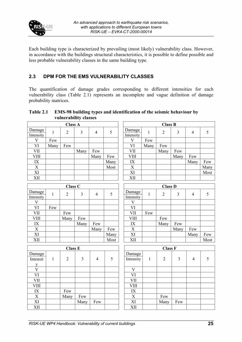
2.3 DPM FOR THE EMS VULNERABILITY CLASSES The quantification of damage grades corresponding to different intensities for each vulnerability class (Table 2.1) represents an incomplete and vague definition of damage probability matrices. Table 2.1 EMS-98 building types and identification of the seismic behaviour by
vulnerability classes Class A Class B
Damage DamageIntensity 1 2 3 4 5
Intensity 1 2 3 4 5
V Few V Few VI Many Few VI Many Few VII Many Few VII Many Few VIII Many Few VIII Many Few IX Many IX Many Few X Most X ManyXI XI Most XII XII
Class C Class D Damage DamageIntensity 1 2 3 4 5
Intensity 1 2 3 4 5
V V VI Few VI VII Few VII Few VIII Many Few VIII Few IX Many Few IX Many Few X Many Few X Many Few XI Many XI Many Few XII Most XII Most
Class E Class F Damage DamageIntensit
y 1 2 3 4 5
Intensity 1 2 3 4 5
V V VI VI VII VII VIII VIII IX Few IX X Many Few X Few XI Many Few XI Many Few XII XII

An advanced approach to earthquake risk scenarios,
with applications to different European towns RISK-UE – EVK4-CT-2000-00014
RISK-UE WP4 Handbook: Vulnerability of current buildings
26
Beta distribution is used to calculate continuous DPM for every vulnerability class as follows
PDF: ( ) ( )( ) ( )
( ) ( )( ) 1t
1qt1q
abx-ba-x
qt qtxp −
−−−
β−−ΓΓ
Γ= a ≤ x < b (2-1)
CDF: ( ) ( )∫ εε= ββ
x
a
dpxP (2-2)
where: a, b, t and q are the parameters of the distribution, and x is the continuous variable which ranges between a and b. The parameters of the beta distribution are correlated with the mean damage grade µD as follows:
( )D2D
3D 2875.0052.0007.0tq µ+µ−µ= (2-3)
The parameter t affects the scatter of the distribution; and if t=8 is used, the beta distribution looks very similar to the binomial distribution. For use of the beta distribution, it is necessary to make reference to the damage grade D, which is a discrete variable, characterized by 5 damage grades plus the grade zero damage (absence of damage). It is advisable to assign value 0 to the parameter a and value 6 to the parameter b (Lagomarsino et al., 2002). The qualitative definitions of the quantities in EMS-98 damage matrices are interpreted through membership functions χ, that define affiliation of single values of the parameter to a specific set, i.e.,
1. χ = 1, the membership is plausible; 2. χ = 0 – 1, the value of the parameter is rare but possible; and, 3. χ = 0, the parameter doesn’t belong to the set. The membership functions for the quantities (percentage of buildings) named low, many or most are defined by means of a straight line in the vague zones (Fig. 2.1). The plausible values of the parameter µD are the ones for which all EMS-98 quantity definitions are plausible. The possible values of the parameter µD are the ones for which all EMS-98 quantity definitions are still plausible or possible, with at least one which is only possible. Using the above procedure, the plausible and possible bounds of the mean damage grade for each vulnerability class are defined (Fig. 2.2).
2.4 VULNERABILITY INDEX AND SEMI-EMPIRICAL VULNERABILITY CURVES The membership of a building to a specific vulnerability class is defined by a vulnerability index. Its values are arbitrary, as it represents only a score that quantifies the seismic behaviour of the building. The vulnerability index ranges between 0 and 1, being values close

An advanced approach to earthquake risk scenarios,
with applications to different European towns RISK-UE – EVK4-CT-2000-00014
RISK-UE WP4 Handbook: Vulnerability of current buildings
27
to 1 represent the most vulnerable buildings with these close to 0, the vulnerability of the high-code designed structures.
0
0,2
0,4
0,6
0,8
1
0 10 20 30 40 50 60 70 80 90 100
r = % of damaged buildings
Mem
bers
hip
Func
tion
χB
TM
FEW
MANYMOST
Fig. 2.1 Membership functions for the quantities Few, Many, Most
0
1
2
3
4
5
5 6 7 8 9 10 11 12EMS-98 Intensity
Mea
n D
amag
e G
rade
A--A-A+A++B--B-B+B++C--C-C+C++D--D-D+D++E--E-E+E++F--F-F+F++
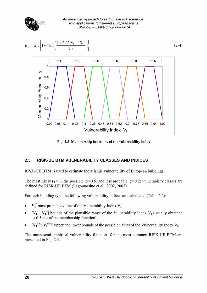
Fig. 2.2 Plausible and possible behaviour for each vulnerability class The membership functions of the six vulnerability classes have a plausible (χ=1) and linear possible ranges, defining the transition between two adjacent classes (Fig. 2.3). The LM1 method defines mean semi-empirical vulnerability functions that correlate the mean damage grade µD with the macroseismic intensity I and the vulnerability index VI. These functions are fitting the DPM's discrete point (Fig. 2.2).
An advanced approach to earthquake risk scenarios,
with applications to different European towns RISK-UE – EVK4-CT-2000-00014
RISK-UE WP4 Handbook: Vulnerability of current buildings
28
−+
+=µ3.2
1.13V 6.25Itanh1 5.2 ID (2-4)
0
0,2
0,4
0,6
0,8
1
-0,02 0,06 0,14 0,22 0,3 0,38 0,46 0,54 0,62 0,7 0,78 0,86 0,94 1,02
Vulnerability Index VI
Mem
bers
hip
Func
tion
χ
F E D C B A
Fig. 2.3 Membership functions of the vulnerability index
2.5 RISK-UE BTM VULNERABILITY CLASSES AND INDICES RISK-UE BTM is used to estimate the seismic vulnerability of European buildings. The most likely (χ=1), the possible (χ=0.6) and less probable (χ=0.2) vulnerability classes are defined for RISK-UE BTM (Lagomarsino et al., 2002, 2003). For each building type the following vulnerability indices are calculated (Table 2.2):
• VI
* most probable value of the Vulnerability Index VI;
• [VI- ; VI
+] bounds of the plausible range of the Vulnerability Index VI (usually obtained as 0.5-cut of the membership function);
• [VImin; VI
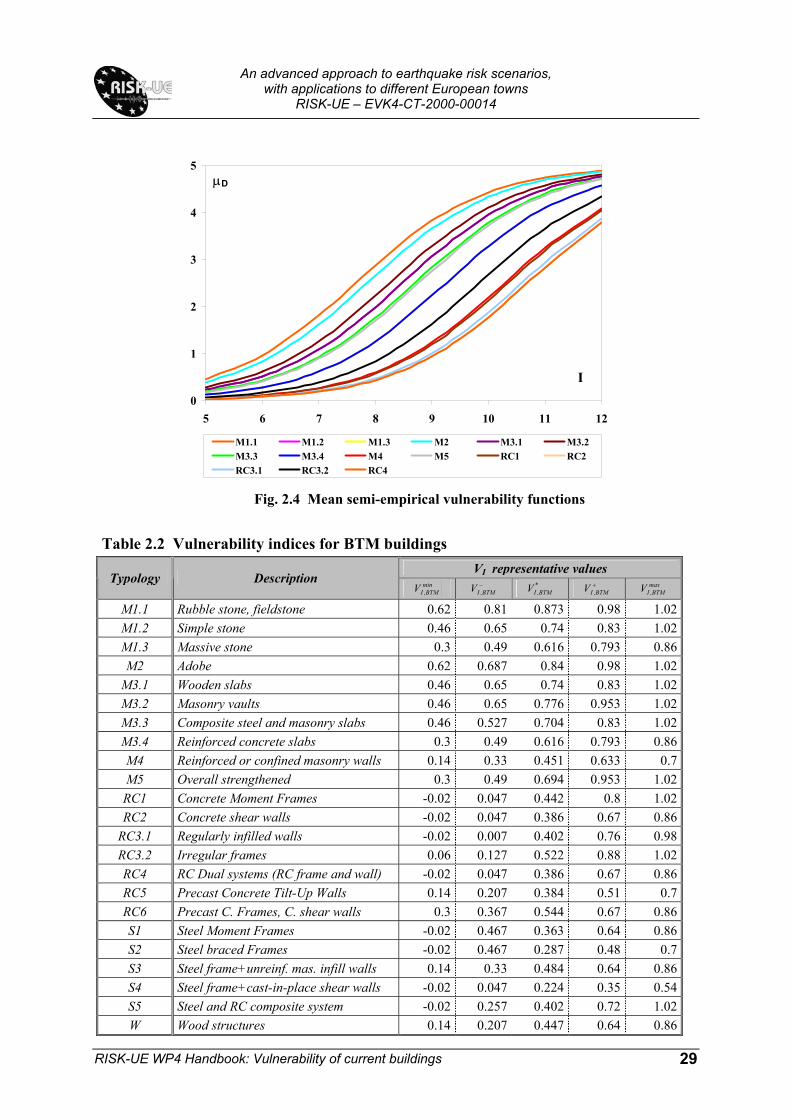
max] upper and lower bounds of the possible values of the Vulnerability Index VI. The mean semi-empirical vulnerability functions for the most common RISK-UE BTM are presented in Fig. 2.4.
An advanced approach to earthquake risk scenarios,
with applications to different European towns RISK-UE – EVK4-CT-2000-00014
RISK-UE WP4 Handbook: Vulnerability of current buildings
29
0
1
2
3
4
5
5 6 7 8 9 10 11 12
M1.1 M1.2 M1.3 M2 M3.1 M3.2M3.3 M3.4 M4 M5 RC1 RC2RC3.1 RC3.2 RC4
µD
I
Fig. 2.4 Mean semi-empirical vulnerability functions
Table 2.2 Vulnerability indices for BTM buildings
VI representative values Typology Description
minBTM,IV −
BTM,IV *BTM,IV +
BTM,IV maxBTM,IV
M1.1 Rubble stone, fieldstone 0.62 0.81 0.873 0.98 1.02M1.2 Simple stone 0.46 0.65 0.74 0.83 1.02M1.3 Massive stone 0.3 0.49 0.616 0.793 0.86M2 Adobe 0.62 0.687 0.84 0.98 1.02
M3.1 Wooden slabs 0.46 0.65 0.74 0.83 1.02M3.2 Masonry vaults 0.46 0.65 0.776 0.953 1.02M3.3 Composite steel and masonry slabs 0.46 0.527 0.704 0.83 1.02M3.4 Reinforced concrete slabs 0.3 0.49 0.616 0.793 0.86M4 Reinforced or confined masonry walls 0.14 0.33 0.451 0.633 0.7M5 Overall strengthened 0.3 0.49 0.694 0.953 1.02RC1 Concrete Moment Frames -0.02 0.047 0.442 0.8 1.02RC2 Concrete shear walls -0.02 0.047 0.386 0.67 0.86
RC3.1 Regularly infilled walls -0.02 0.007 0.402 0.76 0.98RC3.2 Irregular frames 0.06 0.127 0.522 0.88 1.02RC4 RC Dual systems (RC frame and wall) -0.02 0.047 0.386 0.67 0.86RC5 Precast Concrete Tilt-Up Walls 0.14 0.207 0.384 0.51 0.7RC6 Precast C. Frames, C. shear walls 0.3 0.367 0.544 0.67 0.86S1 Steel Moment Frames -0.02 0.467 0.363 0.64 0.86S2 Steel braced Frames -0.02 0.467 0.287 0.48 0.7S3 Steel frame+unreinf. mas. infill walls 0.14 0.33 0.484 0.64 0.86S4 Steel frame+cast-in-place shear walls -0.02 0.047 0.224 0.35 0.54S5 Steel and RC composite system -0.02 0.257 0.402 0.72 1.02W Wood structures 0.14 0.207 0.447 0.64 0.86

An advanced approach to earthquake risk scenarios,
with applications to different European towns RISK-UE – EVK4-CT-2000-00014
RISK-UE WP4 Handbook: Vulnerability of current buildings
30
2.6 VULNERABILITY ANALYSIS
2.6.1 Processing of Available Data Any available database related to buildings must be taken into consideration, classifying the information contained from a geographic and a consistency point of view (Table 2.3). Moreover all the knowledge about observed vulnerability or traditional construction techniques must be collected as well. The distribution, the number and the quality of the available information influence all the parameters involved in the vulnerability analysis.
Table 2.3 Processing of the available data
Data characteristics Consequences Single building Minimum survey
unit Set of buildings Minimum unit to make reference for the VI evaluation.
Single building Geographic
Minimum geocoded unit Set of buildings
Minimum unit for damage and scenarios representations.
Specific survey with vulnerability assessment purposes. Data origin
Other origins
∆Vf
Typological Identifications VI Quality
Data Consistency Behaviour modifiers identifications ∆Vm
Observed Vulnerability Existing Knowledge Expert judgment ∆Vr
2.6.2 Direct and Indirect Typological Identification When a building typology is directly identified within BTM, the vulnerability index values (VI
*, VI- ,VI
+ ,VImin, VI
max) are univocally attributed according to the proposed Table 2.2. If the available data are not enough to perform a direct typological identification it is useful to define more general categories on the base of the experience and the knowledge of the construction tradition. The typological distribution inside the defined categories is supposed to be known. For each category the vulnerability index values (VI
*, VI- ,VI
+ ,VImin, VI
max) are evaluated knowing the percentage of the different building types recognized inside the certain category
*iI
tt
*iI BTMCAT
V pV ∑= (2-5)
where pt is the ratio of buildings inside the category Ci supposing to belong to certain building type..

An advanced approach to earthquake risk scenarios,
with applications to different European towns RISK-UE – EVK4-CT-2000-00014
RISK-UE WP4 Handbook: Vulnerability of current buildings
31
2.6.3 Regional Vulnerability Factor ∆VR A Regional Vulnerability Factor ∆VR is introduced to take into account the particular quality of some building types at a regional level. It modifies the vulnerability index VI
* on a base of an expert judgment or taking into consideration of observed vulnerability. The Regional Vulnerability Factor ∆VR could be introduced both referring to a typology or to a category.
2.6.4 Behaviour Modifier ∆Vm There are different methods that evaluate the vulnerability through the weighted average or the sum of the partial scores to obtain a global score, which practically represents a vulnerability index (ATC-21, GNDT II Level). The proposed procedure is conceptually similar introducing the behaviour modifiers whose values are presented in Tables 2.4 and 2.5. The overall score that modifies the characteristic vulnerability index VI
* can be evaluated, for a single building, simply summing all the modifier scores.
∑=∆ mm VV (2-6)
Table 2.4 Scores for the vulnerability factors Vm: masonry buildings Vulnerability Factors Parameters
Good maintenance -0,04 State of preservation Bad maintenance +0.04 Low (1 or 2) -0.02
Medium (3, 4 or 5) +0.02 Number of floors High (6 or more) +0.06 Wall thickness
Distance between walls Connection between walls (tie-rods, angle bracket) Structural system
Connection horizontal structures-walls
-0,04 ÷ +0,04
Soft-story Demolition/ Transparency +0.04 Plan Irregularity … +0.04
Vertical Irregularity … +0.02 Superimposed floors +0.04
Roof weight + Roof Thrust Roof Roof Connections +0.04
Retrofitting interventions -0,08 ÷ +0,08Aseismic Devices Barbican, Foil arches, Buttresses
Middle -0.04 Corner +0.04 Aggregate building: position Header +0.06
Staggered floors +0.02 Aggregate building: elevation Buildings of different height -0,04 ÷ +0,04
Foundation Different level foundation +0.04 Slope +0.02 Soil Morphology Cliff +0.04

An advanced approach to earthquake risk scenarios,
with applications to different European towns RISK-UE – EVK4-CT-2000-00014
RISK-UE WP4 Handbook: Vulnerability of current buildings
32
For a set of buildings considered belonging to a certain typology, the contribution of each single factor are added, weighing with the ratio of buildings within the set:
∑=∆ k,mkm V rV (2-7) where rk is the ratio of buildings characterized by the modifying factor k, with score Vm,k.
Table 2.5 Scores for the vulnerability factors Vm: R.C. buildings ERD level Vulnerability Factors Pre or Low Code Medium Code High Code
Code Level +0,16 0 -0,16 Bad Maintenance +0.04 +0.02 0
Low (1 or 2) -0,04 -0,04 -0,04 Medium (3, 4 or 5) 0 0 0 Number of floors High (6 or more) +0,08 +0,06 +0,04
Shape +0.04 +0.02 0 Plan Irregularity Torsion +0.02 +0.01 0 Vertical Irregularity +0.04 +0.02 0
Short-column +0.02 +0.01 0 Bow windows +0.04 +0.02 0
Aggregate buildings (insufficient aseismic joint) +0,04 0 0
Beams -0,04 0 0 Connected Beans 0 0 0 Foundation Isolated Footing +0,04 0 0
Slope +0.02 +0.02 +0.02 Soil Morphology Cliff +0.04 +0.04 +0.04
2.6.5 Total vulnerability index The total vulnerability index value is calculated as follows:
mR*II VVVV ∆+∆+= (2-8)
2.6.6 Uncertainty Range Evaluation ∆Vf The knowledge of additional information limits the uncertainty of the building behaviour. Therefore it is advisable not only to modify the most probable value, but also to reduce the range of representative values. This goal is achieved modifying the membership function trough a filter function (f), centered on the new most probable value (VIdef ), depending on the width of the filter function ∆Vf. The width ∆Vf depends on the type of the available data for vulnerability analysis (Table 2.6). The upper and lower bound of the meaningful range of behaviour can be evaluated as follows:

An advanced approach to earthquake risk scenarios,
with applications to different European towns RISK-UE – EVK4-CT-2000-00014
RISK-UE WP4 Handbook: Vulnerability of current buildings
33
fIsupI VVV ∆+= (2-9a)
fIinfI VVV ∆−= (2-9b) Table 2.6 Suggested values for ∆Vf
Single Building
Set of buildings
Non specific existing data base 0.08 0.08 ∆Vf Typology/Category Data surveyed for seismic vulnerability
purposes 0.04 0.04
The VIdef is calculated as follows:
( )fminiinfIIdef VV ;VmaxV ∆+= (2-10a)
( )fmaxisupIIdef VV ;VminV ∆−= (2-10b)
where max
imini V,V are the limits of the membership functions.
2.7. SUMMARY ON DAMAGE ESTIMATION The procedure for damage estimation described in the previous chapters are summarized in the following steps:
STEP 1 – ESTIMATION OF THE VULNERABILITY INDEX VI
Single Building Set of buildings
Typology V*I BTM
Values from Table 2.2 [ ] [ ]BTM BTM
* *I t I
tV Set = q V S.b.⋅∑
qt is the ratio of buildings inside the set supposing to belong to a certain building type
VI*
Category V*I C
cat BTM
* *I i t I t
tV = p V⋅∑
pt is the ratio of buildings inside the category Ci supposing to belong to a certain building type
[ ] [ ]cat cat
* *I c I
cV Set = q V S.b.⋅∑
qc is the ratio of buildings inside the set supposing to belong to a certain building category
∆Vm Typology/Category m mV V ∆ = ∑ m k m,k
kV r V ∆ = ∑
rk is the ratio of buildings characterized by the modifying factor k, with score Vm,k
∆VR Typology/Category RV ∆
Established on base of an expert judgment or available observed vulnerability data
R t R tt
V r V ∆ = ∆∑
Where rt is the ratio of buildings recognized as belonging to a specific typology t affected by the recognized ∆VR t
mR*II VVVV ∆+∆+=

An advanced approach to earthquake risk scenarios,
with applications to different European towns RISK-UE – EVK4-CT-2000-00014
RISK-UE WP4 Handbook: Vulnerability of current buildings
34
STEP 2 – ESTIMATION OF THE MEAN DAMAGE GRADE, µD
The mean damage grade shall be estimated for BTM vulnerability index IV and the corresponding seismic intensity I as follows:
−++=µ
3.21.13V 6.25Itanh1 5.2 I
D (2-4, Repeated)
STEP 3 – ESTIMATION OF THE DAMAGE DISTRIBUTION (Damage Probability Matrix and Fragility Curves)
The damage distribution shall be calculated using the beta distribution.
PDF: ( ) ( )( ) ( )
( ) ( )( ) 1t
1rt1r
abx-ba-x
rt rtxp −
−−−
β −−ΓΓΓ
= a ≤ x < b (2-1, Repeated)
CDF: ( ) ( )∫ εε= ββ
x
a
dpxP (2-2, Repeated)
a=0; b=6; t=8; ( )D
2D
3D 2875.0052.0007.0tr µ+µ−µ= (2-3, Repeated)
The discrete beta density probability function is calculated from the probabilities associated with damage grades k and k+1 (k = 0, 1, 2, 3, 4, 5), as follows
( ) ( )kP1kPpk ββ −+= (2-11) The fragility curve defining the probability of reaching or exceeding certain damage grade are obtained directly from the cumulative probability beta distribution as follows:
( ) ( )kP1DDP k β−=≥ (2-12)

An advanced approach to earthquake risk scenarios,
with applications to different European towns RISK-UE – EVK4-CT-2000-00014
RISK-UE WP4 Handbook: Vulnerability of current buildings
35
3. LM2 Method
3.1. AN OVERVIEW The LM2 Method uses two sets of building resistance/damage models (or functions):
• Capacity Model; and, • Fragility Model.
and an adequate representation of the expected seismic input (or demand) to quantify potential damage to buildings resulting from expected ground shaking. The capacity model, or the capacity (i.e. pushover) curve is an overall force-displacement capacity of the structure that estimates the expected peak response of building at a given demand. Capacity models are developed to represent the first mode response of the building assuming that it is the predominant mode of buildings’ vibration and that it primarily controls the damage genesis and progress. Capacity curves are based on engineering parameters (design, yield, and ultimate structural strength levels) characterizing the nonlinear behaviour of model building classes. They distinguish between materials of construction, construction tradition, experience and technology used, as well as prescribed (by code) and achieved (in practice) levels of seismic protection. Fragility model predicts conditional probabilities for a building of being in (Psk[Ds=ds|Y=yk]) or exceeding (Psk[Ds>ds|Y=yk]) specific damage states (ds) at specified levels of ground motion (yk). In the latter case, the conditional probability of being in a specific damage state is then defined as a difference between adjacent fragility curves. The level and the frequency content of seismic excitation control the peak building response levels, or its performance. The LM2 Method, likely the FEMA/NIBS (1997) procedure, expresses the seismic input in terms of demand spectrum that is based either on the 5% damped building-site specific response spectrum modified to account for structural behaviour out of the elastic domain, or on its alternate, an analogous inelastic response spectrum. The representation of both the capacity (pushover) curve and the demand spectrum is in spectral acceleration (Sa, ordinate) and spectral displacement (Sd, abscissa) coordinate system. This format of presentation is referred as ADRS (Acceleration-Displacement Response Spectra, Mahaney, 1993), or just AD spectra. Adequately, the fragility curves are represented in the coordinate system which abscissa is spectral displacement (Sd) and the ordinate a conditional probability that a particular damage state is meet (P[Ds=ds]) or exceeded (P[Ds>ds]).

An advanced approach to earthquake risk scenarios,
with applications to different European towns RISK-UE – EVK4-CT-2000-00014
RISK-UE WP4 Handbook: Vulnerability of current buildings
36
3.2 BUILDING DAMAGE ASSESSMENT The objective of damage assessment is, for an individual building or a building group, to estimate the expected seismic losses based on sufficiently detailed analysis and evaluation of the vulnerability (damageability) characteristics of the building/building group at a given
level of earthquake ground motions. The conditional probability that particular building or building group will reach certain damage state shall be determined as follows (Fig.3.1):
STEP-1: Select of the model building from the RISK-UE BTM representing adequately buildings’ or buildings’ group characteristics (construction material, structural system, height class, expected/identified design and performance level, etc.);
STEP-2: For selected model building define the capacity model and convert it in capacity spectrum;
STEP-3: Determine/model building’s site-specific demand spectrum;
Fig. 3.1 Damage Estimation Process
Damage States N = None; Mi = Minor; Mo = Moderate; S = Severe; C = Collapse
0
0.1
0.2
0.3
0.4
0.5
N M Mo S C
P[D
=ds]
Performance point
0
0.2
0.4
0.6
0.8
1
Sd (cm)
P[d>
ds]
RISK-UE BTM

An advanced approach to earthquake risk scenarios,
with applications to different European towns RISK-UE – EVK4-CT-2000-00014
RISK-UE WP4 Handbook: Vulnerability of current buildings
37
STEP-4: Calculate/model the expected buildings’ response (performance) by intersecting capacity and demand spectra, and determine the intersection (performance) point; and,
STEP-5: From corresponding fragility model estimate conditional probabilities that for a determined performance point the building or building group will exhibit certain damage states.
The term ‘calculate‘ refers to damage assessment for an individual building, while the term ‘model’ for assessments related to a building class.
3.3 MODELLING CAPACITY CURVES AND CAPACITY SPECTRUM
3.3.1 Capacity Curve A building capacity curve, termed also as ‘pushover’ curve is a function (plot) of a buildings’ lateral load resistance (base shear, V) versus its characteristic lateral displacement (peak building roof displacement, ∆R). Building capacity model is an idealized building capacity curve defined by two characteristic control points: 1) Yield capacity, and 2) Ultimate capacity, i.e.:
Yield capacity (YC, Fig. 3.2-1) is the lateral load resistance strength of the building before structural system has developed nonlinear response. When defining factors like redundancies in design, conservatism in code requirements and true (rather than nominal as defined by standards for code designed and constructed buildings) strength of materials have to be considered. Ultimate capacity (UC, Fig. 3.2-1) is the maximum strength of the building when the global structural system has reached a fully plastic state. Beyond the ultimate point buildings are
Fig. 3.2-1 Building Capacity Model
Ultimate Capacity (UC)
Yield Capacity (YC)
Design Capacity (DC)
∆R ∆u ∆y ∆d λ∆y
Vd
Vy
Vu
V

An advanced approach to earthquake risk scenarios,
with applications to different European towns RISK-UE – EVK4-CT-2000-00014
RISK-UE WP4 Handbook: Vulnerability of current buildings
38
assumed capable of deforming without loss of stability, but their structural system provides no additional resistance to lateral earthquake force. Both, YC and UC control points are defined as:
YC (Vy, ∆y): sy CV γ= 224
TVy
y π=∆ (3-1a)
UC (Vu, ∆u): syu CVV λγλ == 2
2
4πλµγλµ TCsyu =∆=∆ (3-1b)
where: Cs design strength coefficient (fraction of building’s weight), T true “elastic” fundamental-mode period of building (in seconds), γ “overstrength” factor relating design strength to “true” yield strength, λ “overstrength” factor relating ultimate strength to yield strength, and µ “ductility” factor relating ultimate (∆u) displacement to λ times the yield (∆y)
displacement (i.e., assumed point of significant yielding of the structure) Up to the yield point, the building capacity is assumed to be linear with stiffness based on an estimate of the true period of the building. From the yield point to the ultimate point, the capacity curve transitions in slope from an essentially elastic state to a fully plastic state. Beyond the ultimate point the capacity curve is assumed to remain plastic. In countries with developed seismic codes and other construction standards, and rigorous legal system assuring their strict implementation, the design strength, Cs is based on prescribed lateral-force design requirements. It is a function of the seismic zone and other factors including site soil conditions, the type of lateral-force-resisting system and building period. However, the design strength of pre-code buildings, and/or in construction environments characterized with ether bare implementation of design standards and seismic codes or improper monitoring of their implementation, is dominantly controlled by local construction tradition and practice as well as quality of locally available construction materials. The overstrength (γ, λ) and ductility (µ) parameters are defined by the code requirements, based on experimental/empirical evidence and/or on an expert judgment. Building capacity curves could be developed either analytically, based on proper formulation and true nonlinear (Response History Analysis, RHA) or nonlinear static (NSP) analyses of formulated analytical prototypes of model buildings, or on the basis of the best expert’s estimates on parameters controlling the building performance. The latter method, based on parameter estimates prescribed by seismic design codes and construction material standards, in the following is referred as the Code Based Approach (CBA). Chapter 4 details approaches used by RISK-UE partners to develop capacity curves for characteristic model building types being the distinctive features of European built environment.

An advanced approach to earthquake risk scenarios,
with applications to different European towns RISK-UE – EVK4-CT-2000-00014
RISK-UE WP4 Handbook: Vulnerability of current buildings
39
3.3.2 Capacity Spectrum For assuring direct comparison of building capacity and the demand spectrum as well as to facilitate the determination of performance point, base shear (V) is converted to spectral acceleration (Sa) and the roof displacement (∆R) into spectral displacement (Sd). The capacity model of a model structure presented in AD format (Fig. 3.2-2) is termed Capacity Spectrum (Freeman, 1975, 1998). To enable estimation of appropriate reduction of spectral demand, bilinear form of the capacity spectrum is usually used for its either graphical (Fig. 3.2-2) or numerical [(Ay, Dy) and (Au, Du), Eqs. 3-2] representation. Conversion of capacity model (V, ∆R) to capacity spectrum shall be accomplished by knowing the dynamic characteristics of the structure in terms of its period (T), mode shape (φi) and lumped floor mass (mi). For this, a single degree of freedom system (SDOF) is used to represent a translational vibration mode of the structure. Two typical control points, i.e., yield capacity and ultimate capacity, define the Capacity spectrum (Fig. 3.2-2):
YC (Ay, Dy): 1αγs
ayyC
SA == 224
TA
SD ydyy π
== (3-2a)
UC (Au, Du): 1αγ
λλ syauu
CASA ===
2
2
1 4παγ
λµλµ TCDSD s
yduu === (3-2b)
Fig. 3.2-2 Building Capacity Spectrum
Ultimate Capacity (UC)
Yield Capacity (YC)
Design Capacity (DC)

An advanced approach to earthquake risk scenarios,
with applications to different European towns RISK-UE – EVK4-CT-2000-00014
RISK-UE WP4 Handbook: Vulnerability of current buildings
40
where α1is an effective mass coefficient (or fraction of building weight effective in push-over mode), defined with the buildings modal characteristics as follows
[ ]∑ ∑
∑φ
φ=α 2
iii
2ii
1mm
m (3-3)
where: mi is i-th story masses, and φI I-th story modal shape coefficient. Based on first mode vibration properties of vast majority of structures, literature suggests even more simplified approaches. Each mode of an MDOF system can be represented by an equivalent SDOF system with effective mass (Meff) equalling to
MM 1eff α= (3-4) where M is the total mass of the structure. When the equivalent mass of SDOF moves for distance Sd, the roof of the multi-storey building will move for distance ∆R. Considering that the first mode dominantly controls the response of the multi-storey buildings, the ratio of ∆R/Sd = PFR1 is, by definition the modal participation for the fundamental (first) mode at a roof level of MDOF system:
∑ ∑ φφφ= 1R2111R )m/m(PF (3-5)
where φR1 is the first mode shape at the roof level of MDOF system. For most multi-storey buildings Freeman (1998) suggest α1 ≈ 0.80 and PFφR ≈ 1.4. Consequently, Sa = γ [V/(α1Mg)] and Sd = γ (∆R/PFφR) can be estimated at Sa = 1.25 γ Cs (3-6a) Sd = γ ∆R/1.4 (3-6b) Based on analysis of 17 RC multi-storey buildings, Milutinovic and Trendafiloski (2002) estimated α1 = 0.73 and PFφR = 1.33 (σα1 = 0.05, σPFφR = 0.02) for RC frame and α1 = 0.71 and PFφR = 1.47 (σα1 = 0.04, σPFφR = 0.09) for RC dual-system buildings. To define quantitatively the capacity model and the related AD spectrum, five parameters are to be known or estimated:
1) Design strength (Cs); 2) Overstrength factors γ and λ; 3) Ultimate point ductility (µ); and, 4) Typical elastic period of the structure T.

An advanced approach to earthquake risk scenarios,
with applications to different European towns RISK-UE – EVK4-CT-2000-00014
RISK-UE WP4 Handbook: Vulnerability of current buildings
41
The capacity model parameters (Ay, Dy and Au, Du) developed analytically for model buildings constituting the RISK-UE BTM being identified in RISK-UE cities are presented in Tables 3.1. Tables 3.2 summarize the capacity model parameters estimated by IZIIS and UTCB based on expert judgement of Cs, γ, λ, µ and T parameters prescribed by seismic codes and other accompanied standards. In the following these models are referred as CBA (Code Based Approach) capacity as well as fragility models. Graphic presentations of analytically and CBA developed capacity models are given in Appendix A. The fundamental period of the buildings (T) can be estimated using empirically developed formulas (Table 3.3) modified to reflect true structural properties. For code designed buildings Cs and γ are prescribed and can be estimated with relatively high confidence. Displacement control codes with limitations on interstory drift and roof displacement for design and control earthquake levels prescribe the maximum allowable ductility (µ). Force control codes have no such limitations, so µ should be decided based on the experimental data, or by expert judgment. The capacity models and related capacity spectra as well, need not to be exact in order to be useful. A reasonable approximation of the yield and of the ultimate strengths will give a general idea how the building will respond to various earthquake demands. Consequently, the estimates on capacity of each building or building class should be based on the best estimates of typical design parameters (yield and ultimate strengths) used in its design and construction. Even within the same construction-material building category the design parameters can vary substantially. For pre-code buildings they are dependent on engineering tradition and construction practice, while for Code designed buildings, on standards in effect at time of buildings’ design and construction.
3.4 MODELLING FRAGILITY A building fragility model (Fig. 3.3) consists of a suite of fragility curves defining the conditional probability of being in P[D=ds] or exceeding P[D>ds] a certain damage state ds. LM2 method considers four damage states denoted as: Minor, Moderate, Severe and Collapse (Table 1.4). Each fragility curve from a fragility model is characterized by the median value and the lognormal standard deviation (β) of seismic hazard parameter; i.e., the spectral displacement Sd:
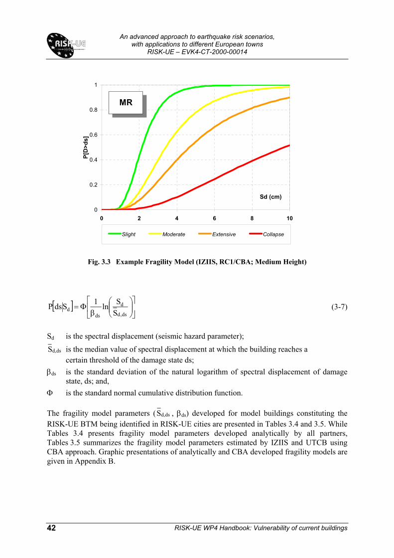
An advanced approach to earthquake risk scenarios,
with applications to different European towns RISK-UE – EVK4-CT-2000-00014
RISK-UE WP4 Handbook: Vulnerability of current buildings
42
[ ]
β
Φ=ds,d
d
dsd S
Sln1SdsP (3-7)
Sd is the spectral displacement (seismic hazard parameter);
dsd,S is the median value of spectral displacement at which the building reaches a certain threshold of the damage state ds; βds is the standard deviation of the natural logarithm of spectral displacement of damage
state, ds; and, Φ is the standard normal cumulative distribution function. The fragility model parameters ( dsd,S , βds) developed for model buildings constituting the RISK-UE BTM being identified in RISK-UE cities are presented in Tables 3.4 and 3.5. While Tables 3.4 presents fragility model parameters developed analytically by all partners, Tables 3.5 summarizes the fragility model parameters estimated by IZIIS and UTCB using CBA approach. Graphic presentations of analytically and CBA developed fragility models are given in Appendix B.
0
0.2
0.4
0.6
0.8
1
0 2 4 6 8 10
Sd (cm)
P[D
>ds]
Slight Moderate Extensive Collapse
MR
Fig. 3.3 Example Fragility Model (IZIIS, RC1/CBA; Medium Height)

An advanced approach to earthquake risk scenarios,
with applications to different European towns RISK-UE – EVK4-CT-2000-00014
RISK-UE WP4 Handbook: Vulnerability of current buildings
43
RISK-UE partners used several methods to define median values of structural fragility:
Masonry buildings: the median values of structural fragility (AUTh, UNIGE and CIMNE) are based on building drift ratios that describe the threshold of damage states (Table 3.6).
RC buildings:
IZIIS, UTCB: the median values of structural fragility are based on correlation between the damage index and the damage state thresholds as defined by Park, Ang & Wen (1992), CIMNE: the median values of structural fragility are based on building drift ratios that describe the threshold of damage states (Table 3.6).
AUTh: Hybrid method, under development. UNIGE: Under development
The original FEMA/NIBS approach proposes that the median values of structural fragility are based on building drift ratios that describe the threshold of damage states. Damage-state drift ratios are converted to spectral displacement by using the following equation:
dsd,S = δR,Sds α2 h (3-8) where: δR,Sds is the drift ratio at the threshold of structural damage state, ds α2 is the fraction of the building (roof) height at the location of pushover model
displacement h is the typical height of the model building type of interest. Building drift ratios are different for each model building type (including height-defined sub-types) and seismic design level. It was used by UTCB for development of fragility models for RC1 and RC2 buildings, only. The total variability associated to each structural damage state βSds, is modelled by combination of three contributors to structural damage variability βC, βD and βM(Sds). The original FEMA/NIBS method assumes that the variability of building response depends jointly on demand and capacity, thus a complex process of convolving probability distributions (Eq. 3-9) of the demand spectrum and the capacity curve (model) has been implemented in developing HAZUS.
( )[ ] ( )2)Sds(M2
DCSds ,CONV β+ββ=β (3-9)
where: βSds is the lognormal standard deviation that describes the total variability for structural
damage state, ds, βC is the lognormal standard deviation parameter that describes the variability of the
capacity curve,

An advanced approach to earthquake risk scenarios,
with applications to different European towns RISK-UE – EVK4-CT-2000-00014
RISK-UE WP4 Handbook: Vulnerability of current buildings
44
βD is the lognormal standard deviation parameter that describes the variability of the demand spectrum,
βM(Sds) is the lognormal standard deviation parameter that describes the uncertainty in the estimate of the median value of the threshold of structural damage state, ds.
However, UTCB assumed that the capacity and demand as independent variables, and modelled the total variability as a RMS value of all three uncertainty contributors (Eq. 3-10).
( )2)Sds(M2
D2
CSds β+β+β=β (3-10) IZIIS used Nonlinear Response History Analysis (NRHA) to develop capacity and associated fragility models for RC1 and RC4 model building classes. Assuming strain-hardening constitution law, the NRHA analyses have been performed for 26 different RC1 and RC4 real buildings by using 7 selected time histories characteristic for the territory of FYRoM and 25 acceleration levels varied from 0.02g to 0.55g. The lognormal standard deviation, ranging from 0.30-0.60 has directly been obtained from the aggregate results of NRHA analyses. To obtain the standard deviation corresponding to each spectral displacement CIMNE and UNIGE assumed that the probability of each damage state at its spectral displacement is the 50% and that the probability of the other damage states are following the same beta distribution used in the LM1 method. Summary overview of techniques used by different WP4 partners for development of fragility models is presented in Table 3.8. The more detailed discussion is presented in Chapter 4.
3.5 DEMAND SPECTRUM The level and frequency content of seismic excitation controls the peak building response. The elastic response spectrum (Sae) is an extremely useful toll characterizing ground motions demand. It also provides convenient means to summarize the peak responses of all possible linear SDOF systems to a particular component of ground motion. It is usually computed for 5 percent damping being representative for a waist majority of structures.
3.5.1 General procedure The application of the Capacity Spectrum technique requires that both, the structural capacity and the demand spectra (elastic spectra reduced for developed level of nonlinearity) be defined in AD (spectral acceleration vs. spectral displacement) coordinate system. General procedure for developing demand spectrum assumes: STEP 1: Calculation of elastic, 5 percent damped, site-specific demand spectrum for
selected period range or a set of discrete period values; STEP 2: For buildings with elastic damping radically different than 5 percent, the 5
percent damped site-specific demand spectrum should either be modified, or a new elastic spectrum calculated by considering the proper damping ratio;

An advanced approach to earthquake risk scenarios,
with applications to different European towns RISK-UE – EVK4-CT-2000-00014
RISK-UE WP4 Handbook: Vulnerability of current buildings
45
STEP 3: Conversion of elastic demand spectrum in AD format. STEP 4: Reduction of elastic AD demand spectrum to account for developed
nonlinearity. Traditionally the elastic seismic demand is defined in the form of an elastic pseudo-acceleration spectrum (Sae) which ordinates [Sae(T)] are directly linked to corresponding ordinates of elastic displacement spectra [Sde(T)] by factor (T2/4π2). While, for defining the elastic demand any spectrum form can be used, the most convenient one is of Newmark-Hall type, i.e., a spectrum with constant acceleration, constant velocity and constant displacement regions.
3.5.2 Elastic Demand Spectrum, RISK-UE Approach The method of developing of 5 percent-damped response/demand spectra is detailed in WP2 Handbook. For RISK-UE Cities 5 percent-damped response/demand spectra are calculated by using Ambraseys 1996 attenuation law. To each grid cell discretizing the urban area assigned are Sae(Ti) values for characteristic discrete period values of Ti = 0., 0.3, 0.6, 1.0 and 2.0 s., and adequate city’s’ zoning has been performed. Over the period range of interest for building damage/loss assessments a model and procedure for calculating 5 percent-damped demand spectra is developed by UNIGE (Lagomarsino et. al., 2002). Based on limited number of known [Sae(T), T] pairs a full period range demand spectra can be fitted by a set of piecewise anchored linear and nonlinear segments:
( )
( ) ( )( ) ( )
( )( ) ( )
≥
≤<≤<≤
≤<≤−
−+−
=−
DD
D
DkiCki
TTi
i
Ckkiik
ikikki
ae
TTTT
TTTTTTTTT
TTTTTTT
TTT
ATS ik
ik
2
/log/log
β
β
ββββ
ββ
(3-11)
where:
Sae(T) is the ordinate of the elastic response spectrum T is the vibration period of linear SDOF A is the peak ground acceleration Ti, Tk is an initial and a final period of each period range TC is a corner period at the beginning of constant velocity region TD is a corner period at the beginning of constant displacement region βi,k,D is factor defined as Sae(Ti,k,D)/A The advantage of such formulation (Eq. 3-11) is that within the acceleration region (0.0 ≤ T ≤ TC) the acceleration is not necessarily constant and may be varied linearly between one or more arbitrary defined points (Fig. 3.4-1). The model in itself assures for flexibility in modelling spectral shapes predominated by intermediate and longer period content. Typical example of such spectral shape is a spectrum developed for the City of Bucharest.

An advanced approach to earthquake risk scenarios,
with applications to different European towns RISK-UE – EVK4-CT-2000-00014
RISK-UE WP4 Handbook: Vulnerability of current buildings
46
For predefined corner periods TC = 0.4s and TD = 2.85s, and arbitrary period selected to comply with the corner period of acceleration region (TB=0.1s) Irizarry et al., 2003 tested the constant acceleration fitting reliability of Lagomarsino et. al. 2003 formulation for Barcelona soil conditions. Results compared to those derived by simplified Eurocode 8 formulation encountered lower RMS and percentage error.
Summary on Construction of Elastic Demand Spectra, Sae(T) STEP 1: Define corner periods and corresponding spectral ordinates for the beginning of
constant velocity (TC) and constant displacement (TD) ranges; STEP 2: Define corner periods and corresponding spectral ordinates
[Ti, Sae(Ti), i=1, 2, .., N] that provide the best piecewise-linear fit to calculated spectra over the constant acceleration range;
STEP 3: For spectral values [Sae(Tj)] calculated for characteristic discrete period values of
Tj, j = 1, 2, …, M, define spectral acceleration values over the constant velocity (TC < T < TD) and constant displacement (T > TD) ranges by using equations 3-11.
3.5.3 AD Conversion of Elastic Demand Spectrum For an elastic SDOF system the following relation applies between the pseudo acceleration (Sae) and displacement (Sde) response spectra:
( ) ( ) 224
TTS
TS aede π
= (3-12)
Thus, each spectral acceleration ordinate associated to period T, is converted into corresponding spectral displacement ordinate by multiplying it with a factor T2/4π2. The Sea/Sde plot, as presented in Fig. 3.4-2, is usually referred to as seismic demand in AD format.
0
1
2
3
4
5
6
7
8
9
10
11
0 0.1 0.2 0.3 0.4 0.5 0.6
Sd (m)
BucharestThessalonikiNice
0
1
2
3
4
5
6
7
8
9
10
11
0 0.25 0.5 0.75 1 1.25 1.5 1.75 2 2.25 2.5 2.75 3
T (s)
Buchar est
Thessal oni ki
Ni ce
Fig. 3.4-1 5% Damped Elastic Demand Spectra
Fig. 3.4-2 5% Damped Elastic Demand Spectra in AD Format
T1
T2 TC
TD
TC
TC

An advanced approach to earthquake risk scenarios,
with applications to different European towns RISK-UE – EVK4-CT-2000-00014
RISK-UE WP4 Handbook: Vulnerability of current buildings
47
3.5.4 Ductility Strength Reduction of AD Demand Spectrum The acceleration spectrum [Sa(T)] and the displacement spectrum [Sd(T)] for an inelastic SDOF system of a bilinear force-deformation relationship are defined as (Vidic et al., 1994):
( ) ( )µRTS
TS aea =
(3-13)
( ) ( ) )(4 2
2
TSTTSR
TS aded πµµ
µ
==
where;
µ is the ductility factor, defined as the ratio between the maximum displacement and the yield displacement; and,
Rµ is strength reduction factor due to ductility, counting for hysteretic energy dissipation of ductile structures.
For selected damping ratio and predefined ductility, the Rµ factor converts the elastic response spectrum [Sae(T)] to the corresponding nonlinear one [Sa(T)]. Since Sa(T) or Sd(T) are defined for predefined value of µ, they are often referred as constant ductility spectra. Several proposals (Miranda, 1996; Cosenza and Manfredi, 1997; Fajfar and Vidic, 2000) have been made for the Rµ factor (Table 3.7, Fig. 3.5). Some of the proposals (Fajfar and Vidic, 2000) use bilinear strength reduction representation or a combination of nonlinear (constant acceleration range) and linear (constant velocity and displacement ranges) segments (Cosenza
0
1
2
3
4
5
6
7
8
9
10
0 0.4 0.8 1.2 1.6 2
T
F-2 F-4 F-6 F-8 C-2 C-4C-6 C-8 M-2 M-4 M-6 M-8
Rµ µ=8
µ=6
µ=4
µ=2
Fig. 3.5 Strength Reduction Factors /F - Fajfar and Vidic, 2000; C - Cosenza and Manfredi, 1997; M - Miranda, 1996./

An advanced approach to earthquake risk scenarios,
with applications to different European towns RISK-UE – EVK4-CT-2000-00014
RISK-UE WP4 Handbook: Vulnerability of current buildings
48
and Manfredi, 1997) anchored at the corner period at the beginning of the constant velocity range (TC = T1, Table 3.7); whereas Mirandas’, 1996 model, distinguishing for site-soil conditions, is nonlinear over the entire period range. Irrespective of the modelling approach, the strength reduction factor estimates are close to each other and agree fairly well. Because of its simplicity, RISK-UE uses bilinear representation of the strength reduction factor Rµ (Vidic et al, 1994; Fajfar, 2000):
( )1 1 CC
C
TR T TT
R T T
µ
µ
µ
µ
= − + < = ≥
(3-14)
where TC is a characteristic period of the ground motion, typically defined as the transition period where the constant acceleration segment of the response spectrum passes to the constant velocity segment (corner period at the beginning of constant velocity range). A typical value of TC, as proposed by Faifar, 2000 is TC = 0.6s, or TC = 0.7s (Cosenza and Manfredi, 1997).
3.5.5 Seismic Demand for Equivalent SDOF System The capacity spectrum method initially characterises seismic demand by an elastic response spectrum. Converted and plotted in AD format it shows the spectral accelerations as a function of spectral displacements. The AD format allows the demand spectrum to be “overlaid” on the buildings’ capacity spectrum. The intersection of the demand and capacity spectra is seismic demand [from the structure]. It represents a point where demand and capacity are equal, and often is termed building ‘performance’ point, or simply ‘Performance Point’. The location of the performance point must satisfy two conditions:
1. The point must lie on the capacity spectrum curve in order to represent the structure at the given displacement; and,
2. The point must lie on a spectral demand curve, reduced from the elastic 5 percent damped response spectrum, that represents the nonlinear demand at the same structural displacement.
If the performance point is located in the linear range of the capacity, it defines the actual displacement of the structure. This is not normally the case as most structures experience inelastic (nonlinear) behaviour when exposed to strong seismic action. For seismic inputs being of interest for damage/loss assessment, the performance points will regularly be out of linear, i.e., in inelastic (nonlinear) capacity range. When the performance point is located in the nonlinear range of the capacity, in the general case, determination of the performance point requires a trial and error search for satisfying the two criteria specified above. In the following, presented are three alternate procedures. All are based on the same concepts and mathematical relations, but vary in assumptions made in solution process and the dependence on graphical versus analytical techniques.

An advanced approach to earthquake risk scenarios,
with applications to different European towns RISK-UE – EVK4-CT-2000-00014
RISK-UE WP4 Handbook: Vulnerability of current buildings
49

An advanced approach to earthquake risk scenarios,
with applications to different European towns RISK-UE – EVK4-CT-2000-00014
RISK-UE WP4 Handbook: Vulnerability of current buildings
50
Performance Point for General Form of Capacity Spectra Term ‘General Form of Capacity Spectra’ assumes a capacity spectra of linear form until the yield point and nonlinear post-yield segment. The procedure presented below is designed as hand or spreadsheet iteration method of converging on the performance point. To define performance point a trial point (SdTR, SaTR) on the capacity spectrum should be selected as an initial estimate. A first choice of trial point could be the displacement obtained using the equal displacement approximation (Fig. 3.6-1), or, it may be the end point of capacity spectrum, or, any other point chosen based on the expert judgement. Based on the spectral acceleration and the spectral displacement defining the trial point (SdTR, SaTR), the strength reduction factor accounting for nonlinear effects associated with it shall be calculated, and then, the demand spectra reduced for calculated strength reduction. The reduced demand spectrum intersects the capacity spectrum at (SdNEW, SaNEW) point. If the displacement at the intersection is equal to initially assumed (SdTR), or is within 5 percent (0.95SdTR ≤ SdNW ≤ 1.05SdTR) of the displacement of the trial performance point, the point (SdNEW, SaNEW) is the performance point, i.e., the unique point where the capacity equals demand.
If the demand spectrum does not intersect the capacity spectrum within the acceptable tolerance, a new trial point shall be selected and the procedure repeated until the accepted tolerance is reached. The choice of a new trial point might be the intersection point determined in the previous step (SdTR = SdNEW, SaTR = SaNEW), or any other point chosen based on expert judgement. For more detailed discussion on the approach the reader is refered to Chapter 8 of ATC-40 document.
Fig. 3.6-1 General Spectrum Procedure
Initial SdTR, SaTR point chosen based on equal displacement approximation
Te
SaTR
Spectral Displacement, cm
SdTR
Capacity Spectrum
5% damped response spectrum
Spec
tral
Acc
eler
atio
n, g
Sd

An advanced approach to earthquake risk scenarios,
with applications to different European towns RISK-UE – EVK4-CT-2000-00014
RISK-UE WP4 Handbook: Vulnerability of current buildings
51
Performance Point for Bilinear Representation of Capacity Spectrum In the case the capacity spectrum is represented by bilinear shape, as it is the case with developments achieved under RISK-UE, a simplified and more direct approach can be used for defining the performance point (Fig. 3.6-2). It is based on the assumption that not only the initial slope of the bilinear representation of the capacity model remains constant, but also the yield point and the post-yield slope. This simplifying assumption allows a direct solution without drawing multiple demand spectra, i.e.:
STEP 1: Plot the 5 percent damped elastic spectrum and the capacity spectrum on the same chart;
STEP 2: Chose several values of Sd,i, i=1, 2, 3, …, N, such as Sd,i > Sdy, Sd,i+1 > Sd,i STEP 3: For each chosen Sd,i define ductilities µi = Sd,i/Sdy, spectral periods Ti,
Ti = 2π√(Sd,i/Sa,i) and define the spectral range (acceleration Ti < TC, or velocity Ti ≥ TC) where it falls
STEP 4: Calculate strength reduction factors Rµ,i using the appropriate expression of Eqs. 3-14
STEP 5: Calculate reduced spectral accelerations (Sa,i) by reducing the corresponding 5% damped elastic spectral accelerations (Sae,i) for adequate strength reduction factor Rµ,i;
iiaeia RSS ,,, / µ= (3-15)
STEP 6: Plot the calculated discrete acceleration/displacement spectral values (Sd,i, Sa,i)
and draw a line connecting plotted points. The intersection of this piecewise linear
Fig. 3.6-2 Capacity Spectrum Procedurefor Bilinear Capacity Model
Spec
tral
Acc
eler
atio
n, g
Spectral Displacement, cm
5% damped response spectrum
Capacity Spectrum Sap
SaY
Performance point at intersection ofCapacity spectrum and line plotted as specified in step 6
Line connecting points plotted as specified in step 6
Te
DY=SdY Sdp Sdi Sd

An advanced approach to earthquake risk scenarios,
with applications to different European towns RISK-UE – EVK4-CT-2000-00014
RISK-UE WP4 Handbook: Vulnerability of current buildings
52
line with the capacity spectrum is the demand spectral displacement, i.e., the performance point.
Although procedure requires plotting of multiple (Sd,i, Sa,i) points, the only (Sd,i, Sa,i) point that has any real significance is the one that lies on the capacity spectrum curve. This point defines the intersection point of the capacity spectrum with the adequate constant damping demand spectrum, and thus defines the demand displacement. It is evident (Fig. 3.6-2) that the (Sd,i, Sa,i) piecewise line steadily slopes down until intersect with the capacity spectrum. This provides opportunity for the procedure to be fully coded and completely automated. Performance Point for Elastic-Perfectly Plastic Representation of Capacity Spectrum While the above-presented procedure also applies, for this particular case (Fig. 3.6-3) there is closed mathematical solution (Fajfer, 2000), thus no plotting is required at all. An estimate on the displacement due to a given seismic demand is made using a simple technique called ‘the equal displacement approximation’. This approximation is based on the assumption that the inelastic spectral displacement (Sd, Fig. 3.6-3) is the same as that which would occur if the structure remained perfectly elastic (Sde).
The intersection of the radial line corresponding to the elastic period [Te, Te = 2π√(Sde/Sae)] of idealized elastic-perfectly plastic system with the elastic 5% damped response spectra (Sae) defines the acceleration (i.e. the strength) and the corresponding displacement (Sde) demands required for elastic (linear) behaviour of the system. The yield acceleration (Say) represents both the acceleration demand and the capacity of the inelastic system. The ratio between the accelerations corresponding to the elastic and inelastic systems represents the strength reduction factor due to ductility, i.e.;
Fig. 3.6-3 Capacity Spectra Procedure -Elastic-Perfectly Plastic Capacity Model
Te<TC
Te>TCTC
5% damped response spectrum
Sd=Sde Sd Dy
Say
Sae
Sa
µ
Dd
Sad
Spectral Displacement, cm
Spec
tral
Acc
eler
atio
n, g
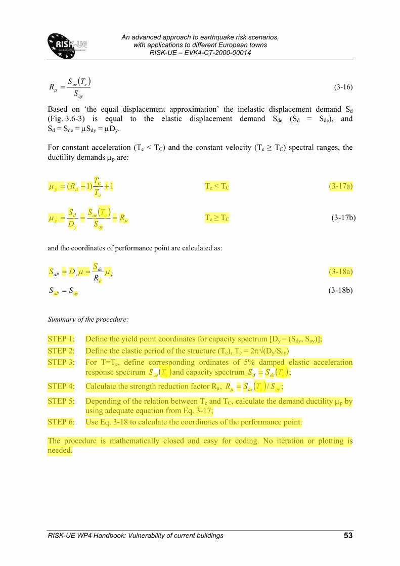
An advanced approach to earthquake risk scenarios,
with applications to different European towns RISK-UE – EVK4-CT-2000-00014
RISK-UE WP4 Handbook: Vulnerability of current buildings
53
( )ay
eae
STS
R =µ (3-16)
Based on ‘the equal displacement approximation’ the inelastic displacement demand Sd (Fig. 3.6-3) is equal to the elastic displacement demand Sde (Sd = Sde), and Sd = Sde = µSdy = µDy. For constant acceleration (Te < TC) and the constant velocity (Te ≥ TC) spectral ranges, the ductility demands µp are:
1)1( +−=e
Cp T
TRµµ Te < TC (3-17a)
( )µµ R
STS
DS
ay
eae
y
dp === Te ≥ TC (3-17b)
and the coordinates of performance point are calculated as:
pde
ydP RS
DS µµµ
== (3-18a)
ayaP SS = (3-18b) Summary of the procedure: STEP 1: Define the yield point coordinates for capacity spectrum [Dy = (Sdy, Say)]; STEP 2: Define the elastic period of the structure (Te), Te = 2π√(Dy/Say) STEP 3: For T=Te, define corresponding ordinates of 5% damped elastic acceleration
response spectrum ( )eae TS and capacity spectrum ( )eded TSS = ;
STEP 4: Calculate the strength reduction factor Rµ, ( ) ayeae STSR /=µ ;
STEP 5: Depending of the relation between Te and TC, calculate the demand ductility µp by using adequate equation from Eq. 3-17;
STEP 6: Use Eq. 3-18 to calculate the coordinates of the performance point. The procedure is mathematically closed and easy for coding. No iteration or plotting is needed.
Francisco Sa
Realce
Francisco Sa
Realce
Francisco Sa
Realce
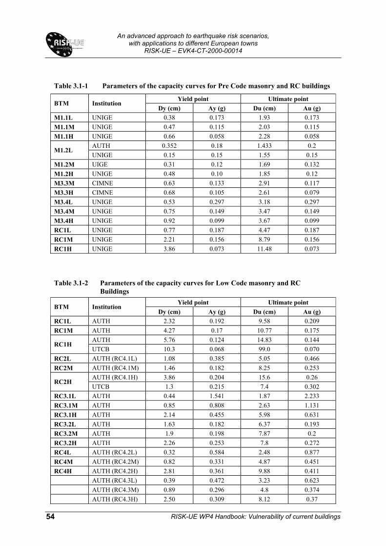
An advanced approach to earthquake risk scenarios,
with applications to different European towns RISK-UE – EVK4-CT-2000-00014
RISK-UE WP4 Handbook: Vulnerability of current buildings
54
Table 3.1-1 Parameters of the capacity curves for Pre Code masonry and RC buildings
Yield point Ultimate point BTM Institution
Dy (cm) Ay (g) Du (cm) Au (g) M1.1L UNIGE 0.38 0.173 1.93 0.173 M1.1M UNIGE 0.47 0.115 2.03 0.115 M1.1H UNIGE 0.66 0.058 2.28 0.058
AUTH 0.352 0.18 1.433 0.2 M1.2L
UNIGE 0.15 0.15 1.55 0.15 M1.2M UIGE 0.31 0.12 1.69 0.132 M1.2H UNIGE 0.48 0.10 1.85 0.12 M3.3M CIMNE 0.63 0.133 2.91 0.117 M3.3H CIMNE 0.68 0.105 2.61 0.079 M3.4L UNIGE 0.53 0.297 3.18 0.297 M3.4M UNIGE 0.75 0.149 3.47 0.149 M3.4H UNIGE 0.92 0.099 3.67 0.099 RC1L UNIGE 0.77 0.187 4.47 0.187 RC1M UNIGE 2.21 0.156 8.79 0.156 RC1H UNIGE 3.86 0.073 11.48 0.073
Table 3.1-2 Parameters of the capacity curves for Low Code masonry and RC Buildings
Yield point Ultimate point BTM Institution
Dy (cm) Ay (g) Du (cm) Au (g) RC1L AUTH 2.32 0.192 9.58 0.209 RC1M AUTH 4.27 0.17 10.77 0.175
AUTH 5.76 0.124 14.83 0.144 RC1H
UTCB 10.3 0.068 99.0 0.070 RC2L AUTH (RC4.1L) 1.08 0.385 5.05 0.466 RC2M AUTH (RC4.1M) 1.46 0.182 8.25 0.253
AUTH (RC4.1H) 3.86 0.204 15.6 0.26 RC2H
UTCB 1.3 0.215 7.4 0.302 RC3.1L AUTH 0.44 1.541 1.87 2.233 RC3.1M AUTH 0.85 0.808 2.63 1.131 RC3.1H AUTH 2.14 0.455 5.98 0.631 RC3.2L AUTH 1.63 0.182 6.37 0.193 RC3.2M AUTH 1.9 0.198 7.87 0.2 RC3.2H AUTH 2.26 0.253 7.8 0.272 RC4L AUTH (RC4.2L) 0.32 0.584 2.48 0.877 RC4M AUTH (RC4.2M) 0.82 0.331 4.87 0.451 RC4H AUTH (RC4.2H) 2.81 0.361 9.88 0.411 AUTH (RC4.3L) 0.39 0.472 3.23 0.623 AUTH (RC4.3M) 0.89 0.296 4.8 0.374 AUTH (RC4.3H) 2.50 0.309 8.12 0.37
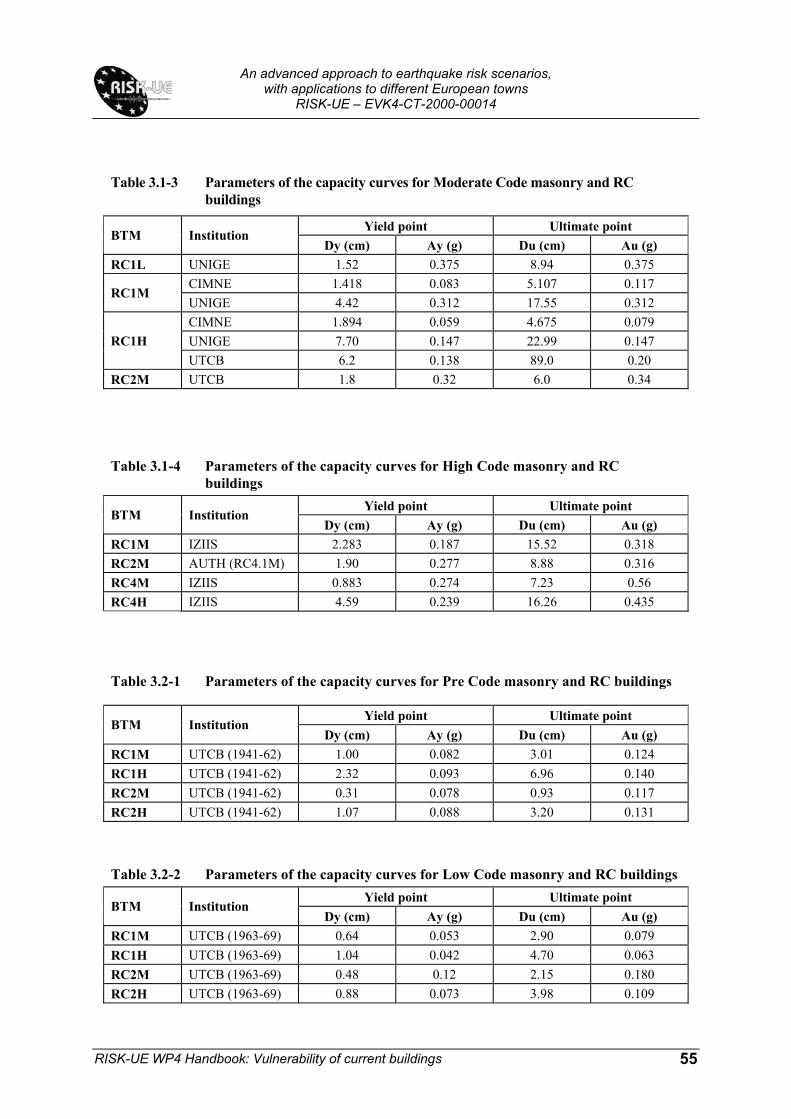
An advanced approach to earthquake risk scenarios,
with applications to different European towns RISK-UE – EVK4-CT-2000-00014
RISK-UE WP4 Handbook: Vulnerability of current buildings
55
Table 3.2-1 Parameters of the capacity curves for Pre Code masonry and RC buildings
Yield point Ultimate point BTM Institution
Dy (cm) Ay (g) Du (cm) Au (g) RC1M UTCB (1941-62) 1.00 0.082 3.01 0.124 RC1H UTCB (1941-62) 2.32 0.093 6.96 0.140 RC2M UTCB (1941-62) 0.31 0.078 0.93 0.117 RC2H UTCB (1941-62) 1.07 0.088 3.20 0.131
Table 3.2-2 Parameters of the capacity curves for Low Code masonry and RC buildings Yield point Ultimate point
BTM Institution Dy (cm) Ay (g) Du (cm) Au (g)
RC1M UTCB (1963-69) 0.64 0.053 2.90 0.079 RC1H UTCB (1963-69) 1.04 0.042 4.70 0.063 RC2M UTCB (1963-69) 0.48 0.12 2.15 0.180 RC2H UTCB (1963-69) 0.88 0.073 3.98 0.109
Table 3.1-3 Parameters of the capacity curves for Moderate Code masonry and RC buildings
Yield point Ultimate point BTM Institution
Dy (cm) Ay (g) Du (cm) Au (g) RC1L UNIGE 1.52 0.375 8.94 0.375
CIMNE 1.418 0.083 5.107 0.117 RC1M
UNIGE 4.42 0.312 17.55 0.312 CIMNE 1.894 0.059 4.675 0.079 UNIGE 7.70 0.147 22.99 0.147 RC1H UTCB 6.2 0.138 89.0 0.20
RC2M UTCB 1.8 0.32 6.0 0.34
Table 3.1-4 Parameters of the capacity curves for High Code masonry and RC buildings
Yield point Ultimate point BTM Institution
Dy (cm) Ay (g) Du (cm) Au (g) RC1M IZIIS 2.283 0.187 15.52 0.318 RC2M AUTH (RC4.1M) 1.90 0.277 8.88 0.316 RC4M IZIIS 0.883 0.274 7.23 0.56 RC4H IZIIS 4.59 0.239 16.26 0.435

An advanced approach to earthquake risk scenarios,
with applications to different European towns RISK-UE – EVK4-CT-2000-00014
RISK-UE WP4 Handbook: Vulnerability of current buildings
56
Table 3.2-3 Parameters of the capacity curves for Moderate Code masonry and RC buildings
Yield point Ultimate point BTM Institution
Dy (cm) Ay (g) Du (cm) Au (g) RC1L IZIIS (1964-81) 0.10 0.18 0.22 0.20
IZIIS (1964-81) 1.51 0.17 3.31 0.19 UTCB (1970-77) 0.68 0.056 3.07 0.084 RC1M UTCB (1978-89) 1.26 0.141 12.63 0.282 IZIIS (1964-81) 3.52 0.10 7.75 0.11 UTCB (1970-77) 1.11 0.045 5.01 0.067 RC1H UTCB (1978-89) 2.87 0.160 28.73 0.320 UTCB (1970-77) 0.45 0.112 2.00 0.168
RC2M UTCB (1978-89) 0.51 0.167 4.06 0.333 UTCB (1970-77) 0.94 0.077 4.22 0.116
RC2H UTCB (1978-89) 1.68 0.188 13.42 0.375
Table 3.2-4 Parameters of the capacity curves for High Code masonry and RC buildings Yield point Ultimate point
BTM Institution Dy (cm) Ay (g) Du (cm) Au (g)
RC1L IZIIS (1981) 0.07 0.13 0.59 0.26 IZIIS (1981) 1.31 0.15 10.44 0.29
RC1M UTCB (1990-02) 1.58 0.176 15.79 0.353 IZIIS (1981) 4.58 0.13 36.63 0.26
RC1H UTCB (1990-02) 3.59 0.200 35.91 0.400
RC2M UTCB (1990-02) 0.63 0.208 5.07 0.417 RC2H UTCB (1990-02) 2.10 0.234 16.77 0.469
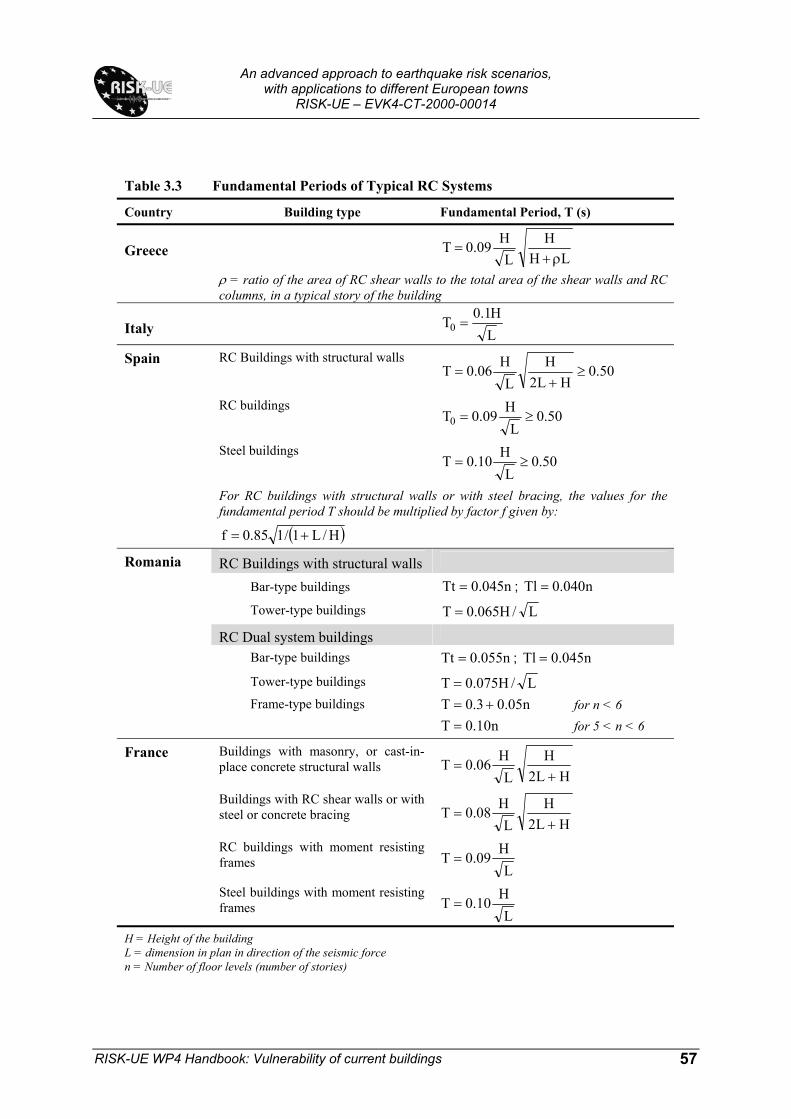
An advanced approach to earthquake risk scenarios,
with applications to different European towns RISK-UE – EVK4-CT-2000-00014
RISK-UE WP4 Handbook: Vulnerability of current buildings
57
Table 3.3 Fundamental Periods of Typical RC Systems
Country Building type Fundamental Period, T (s)
Greece
LHH
LH09.0T
ρ+=
ρ = ratio of the area of RC shear walls to the total area of the shear walls and RC columns, in a typical story of the building
Italy
LH1.0T0 =
Spain RC Buildings with structural walls 50.0
HL2H
LH06.0T ≥
+=
RC buildings 50.0
LH09.0T0 ≥=
Steel buildings 50.0
LH10.0T ≥=
For RC buildings with structural walls or with steel bracing, the values for the fundamental period T should be multiplied by factor f given by:
( )H/L1/185.0f +=
Romania RC Buildings with structural walls
Bar-type buildings n045.0Tt = ; n040.0Tl =
Tower-type buildings L/H065.0T = RC Dual system buildings
Bar-type buildings n055.0Tt = ; n045.0Tl = Tower-type buildings L/H075.0T =
Frame-type buildings n05.03.0T += for n < 6
n10.0T = for 5 < n < 6
France Buildings with masonry, or cast-in-place concrete structural walls
HL2H
LH06.0T
+=
Buildings with RC shear walls or with steel or concrete bracing
HL2H
LH08.0T
+=
RC buildings with moment resisting frames L
H09.0T =
Steel buildings with moment resisting frames L
H10.0T =
H = Height of the building L = dimension in plan in direction of the seismic force n = Number of floor levels (number of stories)

An advanced approach to earthquake risk scenarios,
with applications to different European towns RISK-UE – EVK4-CT-2000-00014
RISK-UE WP4 Handbook: Vulnerability of current buildings
58
Table 3.4-1 Parameters of the fragility curves for Pre Code masonry buildings
Bldg. Properties Spectral Displacements (cm)
Height (m) Interstory drift at
threshold of damage state Slight Moderate Extensive Complete
BT
M
Partn
er
Roo
f
Mod
al
Slig
ht
Mod
erat
e
Exte
nsiv
e
Com
plet
e
Med
ian
Bet
a
Med
ian
Bet
a
Med
ian
Bet
a
Med
ian
Bet
a
M1.2L 4 0.15 0.36 0.71 1.55 M1.2M 4 0.31 0.51 0.86 1.69 M1.2H 4 0.48 0.69 1.03 1.85 M3.3M 2 17.0 0.44 0.40 0.63 0.50 1.20 0.75 2.91 0.70 M3.3H 2 24.0 0.46 0.30 0.68 0.65 1.68 0.65 2.61 0.65
Partners: 1-AUTH; 2-CIMNE; 3-IZIIS; 4-UNIGE; 5-UTCB Table 3.4-2 Parameters of the fragility curves for Low Code masonry and RC buildings
Bldg. Properties Spectral Displacements (cm)
Height (m) Interstory drift at
threshold of damage state Slight Moderate Extensive Complete
BT
M
Partn
er
Roo
f
Mod
al
Slig
ht
Mod
erat
e
Exte
nsiv
e
Com
plet
e
Med
ian
Bet
a
Med
ian
Bet
a
Med
ian
Bet
a
Med
ian
Bet
a
M1.2_1 1 0.145 0.437 0.335 0.656 0.447 0.564 0.64 0.385M1.2_2 1 1.518 0.8 2.466 0.9 3.134 0.7 3.587 0.6M3.4_1 1 0.289 0.85 0.374 0.8 0.468 0.7 0.553 0.65M3.4_2 1 1.686 0.5 2.059 0.5 2.513 0.5 4.090 0.65RC1H 5 37.97 27.94 0.00 0.01 0.01 0.02 7.82 0.65 17.88 0.75 27.94 0.85 68.16 0.95RC2H 5 31.00 21.99 0.02 0.06 0.09 0.24 0.52 0.65 1.30 0.75 2.09 0.85 5.22 0.95
Partners: 1-AUTH; 2-CIMNE; 3-IZIIS; 4-UNIGE; 5-UTCB Table 3.4-3 Parameters of the fragility curves for Moderate Code masonry and RC buildings
Bldg. Properties Spectral Displacements (cm)
Height (m) Interstory drift at
threshold of damage state Slight Moderate Extensive Complete
BT
M
Partn
er
Roo
f
Mod
al
Slig
ht
Mod
erat
e
Exte
nsiv
e
Com
plet
e
Med
ian
Bet
a
Med
ian
Bet
a
Med
ian
Bet
a
Med
ian
Bet
a
RC1M 2 15.8 0.99 0.28 1.42 0.36 2.34 0.50 5.11 0.61RC1H 2 24.0 1.33 0.28 1.89 0.29 2.59 0.34 4.68 0.45RC1H 5 30.8 24.8 0.00 0.01 0.01 0.03 11.67 0.65 21.61 0.75 31.79 0.85 72.03 0.95RC2M 5 22.0 16.2 0.00 0.00 0.00 0.00 0.46 0.65 1.02 0.75 1.58 0.85 3.84 0.95
Partners: 1-AUTH; 2-CIMNE; 3-IZIIS; 4-UNIGE; 5-UTCB

An advanced approach to earthquake risk scenarios,
with applications to different European towns RISK-UE – EVK4-CT-2000-00014
RISK-UE WP4 Handbook: Vulnerability of current buildings
59
Table 3.4-4 Parameters of the feagility curves for High Code RC buildings Bldg. Properties Spectral Displacements (cm)
Height (m) Interstory drift at
threshold of damage state Slight Moderate Extensive Complete
BT
M
Partn
er
Roo
f
Mod
al
Slig
ht
Mod
erat
e
Exte
nsiv
e
Com
plet
e
Med
ian
Bet
a
Med
ian
Bet
a
Med
ian
Bet
a
Med
ian
Bet
a
RC1M 3 2.50 0.50 3.97 0.43 5.18 0.43 10.54 0.51RC4M 3 0.70 0.50 1.27 0.41 1.68 0.40 3.07 0.40RC4H 3 1.97 0.46 3.18 0.33 4.27 0.30 8.72 0.32
Partners: 1-AUTH; 2-CIMNE; 3-IZIIS; 4-UNIGE; 5-UTCB Table 3.5-1 Parameters of the fragility curves for Pre Code RC buildings
Bldg. Properties Spectral Displacements (cm)
Height (m) Interstory drift at
threshold of damage state Slight Moderate Extensive Complete
BT
M
Inst
itutio
n
Roo
f
Mod
al
Slig
ht
Mod
erat
e
Exte
nsiv
e
Com
plet
e
Med
ian
Bet
a
Med
ian
Bet
a
Med
ian
Bet
a
Med
ian
Bet
a
RC1L 5 570 342 0.04 0.08 0.13 0.30 0.14 0.65 0.29 0.75 0.44 0.85 1.03 0.95RC1M 5 1710 1026 0.04 0.08 0.12 0.27 0.38 0.65 0.78 0.75 1.18 0.85 2.79 0.95RC1H 5 2850 1710 0.05 0.11 0.16 0.38 0.87 0.65 1.80 0.75 2.73 0.85 6.46 0.95RC2L 5 570 399 0.00 0.01 0.01 0.03 0.01 0.65 0.03 0.75 0.05 0.85 0.11 0.95RC2M 5 1710 1197 0.01 0.02 0.03 0.07 0.12 0.65 0.24 0.75 0.36 0.85 0.86 0.95RC2H 5 2850 1995 0.02 0.04 0.06 0.15 0.40 0.65 0.83 0.75 1.26 0.85 2.97 0.95
Institutions: 1-AUTH; 2-CIMNE; 3-IZIIS; 4-UNIGE; 5-UTCB
Table 3.5-2 Parameters of the fragility curves for Low Code RC buildings Bldg. Properties Spectral Displacements (cm)
Height (m) Interstory drift at
threshold of damage state Slight Moderate Extensive Complete
BT
M
Inst
itutio
n
Roo
f
Mod
al
Slig
ht
Mod
erat
e
Exte
nsiv
e
Com
plet
e
Med
ian
Bet
a
Med
ian
Bet
a
Med
ian
Bet
a
Med
ian
Bet
a
RC1L 5 570 342 0.06 0.12 0.18 0.43 0.20 0.65 0.41 0.75 0.62 0.85 1.47 0.95RC1M 5 1710 1026 0.03 0.07 0.11 0.25 0.34 0.65 0.71 0.75 1.08 0.85 2.55 0.95RC1H 5 2850 1710 0.03 0.07 0.10 0.24 0.56 0.65 1.15 0.75 1.75 0.85 4.14 0.95RC2L 5 570 399 0.01 0.02 0.03 0.07 0.04 0.65 0.08 0.75 0.12 0.85 0.28 0.95RC2M 5 1710 1197 0.02 0.04 0.07 0.16 0.25 0.65 0.53 0.75 0.80 0.85 1.89 0.95RC2H 5 2850 1995 0.02 0.05 0.07 0.18 0.47 0.65 0.98 0.75 1.48 0.85 3.51 0.95
Institutions: 1-AUTH; 2-CIMNE; 3-IZIIS; 4-UNIGE; 5-UTCB
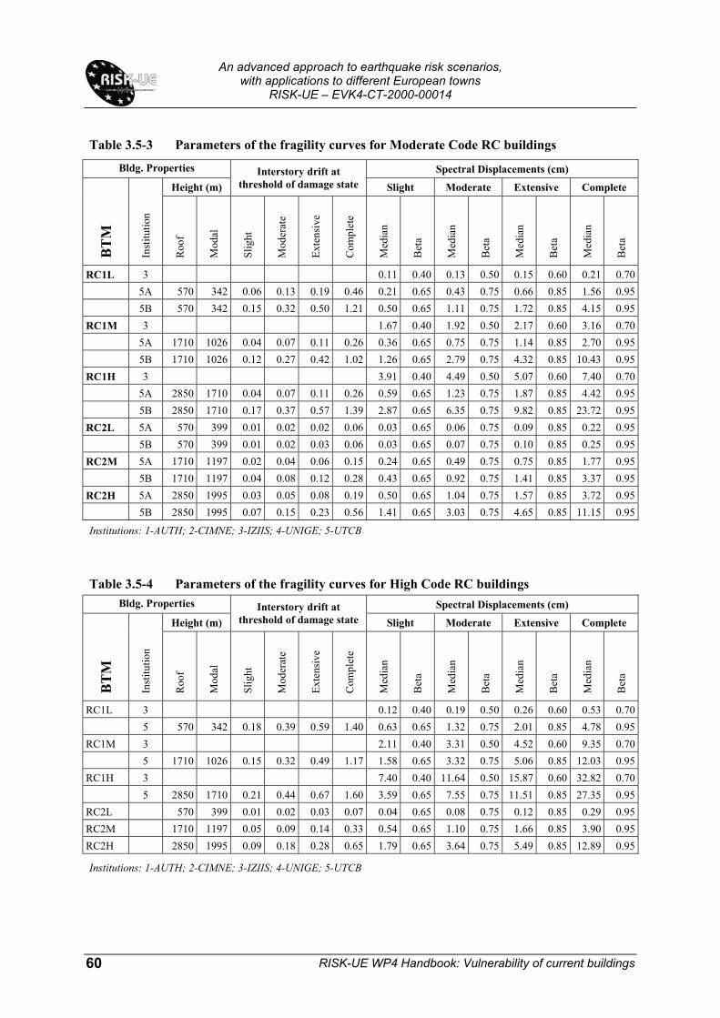
An advanced approach to earthquake risk scenarios,
with applications to different European towns RISK-UE – EVK4-CT-2000-00014
RISK-UE WP4 Handbook: Vulnerability of current buildings
60
Table 3.5-3 Parameters of the fragility curves for Moderate Code RC buildings
Bldg. Properties Spectral Displacements (cm)
Height (m) Interstory drift at
threshold of damage state Slight Moderate Extensive Complete
BT
M
Inst
itutio
n
Roo
f
Mod
al
Slig
ht
Mod
erat
e
Exte
nsiv
e
Com
plet
e
Med
ian
Bet
a
Med
ian
Bet
a
Med
ian
Bet
a
Med
ian
Bet
a
RC1L 3 0.11 0.40 0.13 0.50 0.15 0.60 0.21 0.70 5A 570 342 0.06 0.13 0.19 0.46 0.21 0.65 0.43 0.75 0.66 0.85 1.56 0.95 5B 570 342 0.15 0.32 0.50 1.21 0.50 0.65 1.11 0.75 1.72 0.85 4.15 0.95RC1M 3 1.67 0.40 1.92 0.50 2.17 0.60 3.16 0.70 5A 1710 1026 0.04 0.07 0.11 0.26 0.36 0.65 0.75 0.75 1.14 0.85 2.70 0.95 5B 1710 1026 0.12 0.27 0.42 1.02 1.26 0.65 2.79 0.75 4.32 0.85 10.43 0.95RC1H 3 3.91 0.40 4.49 0.50 5.07 0.60 7.40 0.70 5A 2850 1710 0.04 0.07 0.11 0.26 0.59 0.65 1.23 0.75 1.87 0.85 4.42 0.95 5B 2850 1710 0.17 0.37 0.57 1.39 2.87 0.65 6.35 0.75 9.82 0.85 23.72 0.95RC2L 5A 570 399 0.01 0.02 0.02 0.06 0.03 0.65 0.06 0.75 0.09 0.85 0.22 0.95 5B 570 399 0.01 0.02 0.03 0.06 0.03 0.65 0.07 0.75 0.10 0.85 0.25 0.95RC2M 5A 1710 1197 0.02 0.04 0.06 0.15 0.24 0.65 0.49 0.75 0.75 0.85 1.77 0.95 5B 1710 1197 0.04 0.08 0.12 0.28 0.43 0.65 0.92 0.75 1.41 0.85 3.37 0.95RC2H 5A 2850 1995 0.03 0.05 0.08 0.19 0.50 0.65 1.04 0.75 1.57 0.85 3.72 0.95 5B 2850 1995 0.07 0.15 0.23 0.56 1.41 0.65 3.03 0.75 4.65 0.85 11.15 0.95
Institutions: 1-AUTH; 2-CIMNE; 3-IZIIS; 4-UNIGE; 5-UTCB
Table 3.5-4 Parameters of the fragility curves for High Code RC buildings Bldg. Properties Spectral Displacements (cm)
Height (m) Interstory drift at
threshold of damage state Slight Moderate Extensive Complete
BT
M
Inst
itutio
n
Roo
f
Mod
al
Slig
ht
Mod
erat
e
Exte
nsiv
e
Com
plet
e
Med
ian
Bet
a
Med
ian
Bet
a
Med
ian
Bet
a
Med
ian
Bet
a
RC1L 3 0.12 0.40 0.19 0.50 0.26 0.60 0.53 0.70 5 570 342 0.18 0.39 0.59 1.40 0.63 0.65 1.32 0.75 2.01 0.85 4.78 0.95RC1M 3 2.11 0.40 3.31 0.50 4.52 0.60 9.35 0.70 5 1710 1026 0.15 0.32 0.49 1.17 1.58 0.65 3.32 0.75 5.06 0.85 12.03 0.95RC1H 3 7.40 0.40 11.64 0.50 15.87 0.60 32.82 0.70 5 2850 1710 0.21 0.44 0.67 1.60 3.59 0.65 7.55 0.75 11.51 0.85 27.35 0.95RC2L 570 399 0.01 0.02 0.03 0.07 0.04 0.65 0.08 0.75 0.12 0.85 0.29 0.95RC2M 1710 1197 0.05 0.09 0.14 0.33 0.54 0.65 1.10 0.75 1.66 0.85 3.90 0.95RC2H 2850 1995 0.09 0.18 0.28 0.65 1.79 0.65 3.64 0.75 5.49 0.85 12.89 0.95
Institutions: 1-AUTH; 2-CIMNE; 3-IZIIS; 4-UNIGE; 5-UTCB

An advanced approach to earthquake risk scenarios,
with applications to different European towns RISK-UE – EVK4-CT-2000-00014
RISK-UE WP4 Handbook: Vulnerability of current buildings
61
Dam
age
Gra
de
Definition Displacement Limits (AUTh) Spectral Displacement
Limits (UNIGE, CIMNE)
0 No damage ∆ < 0.7∆y D < 0.7 Dy
1 Slight damage 0.7∆y < ∆ < 0.7∆y+0.05*∆uy 0.7Dy ≤ D < 1.0 Dy
2 Moderate damage 0.7∆y+0.05*∆uy < ∆ < 0.7∆y+0.20*∆uy 1.0 Dy ≤ D < Dy+Duy
3 Extensive damage 0.7∆y+0.20*∆uy < ∆ < 0.7∆y+0.50*∆uy Dy+Duy ≤ D < Du
4 Very heavy damage 0.7∆y+0.50*∆uy < ∆ < 0.7∆y+1.00*∆uy Du ≤ D
∆uy = 0.9∆u-0.7∆y Duy = 0.25*(Du-Dy)
Table 3.7 Strength Reduction Factors
Author Strength reduction factor
Fajfar and Vidic, 2000 (F)
( ) 1TT1R
c+−µ=µ
µ=µR
Cosenza and Manfredi, 1997 (C)
( ) 8.075.0 15.11R −µτ+=µ
1TT
=τ
τ= 1 T > T1
Miranda, 1996 (M)
Φ−µ
+=µ11R
( )[ ]26.0Tln5.1expT21
TT1011 −−−
µ−+=Φ
( )[ ]22.0Tln2expT52
TT1211 −−−
µ−+=Φ
−−−+=Φ
2
S
SS 25.0TTln3exp
T4T3
T3T1
Table 3.6 Building Drift Ratios at the Threshold of Damage States

An advanced approach to earthquake risk scenarios,
with applications to different European towns RISK-UE – EVK4-CT-2000-00014
RISK-UE WP4 Handbook: Vulnerability of current buildings
62
Table 3.8. Principal Steps of Fragility Analysis
Steps Pushover / CBA Nonlinear Dynamic
STEP 1: Define/model capacity spectra (bilinear model)
Define/model dynamic capacity spectra (bilinear model)
STEP 2: Define damage thresshold levels (criteria) Sa
Sd Dy Du
Sd1 Sd2 Sd3 Sd4
( )DuSd
DyDu25.0DySdDySd
Dy7.0Sd
4
3
2
1
=−+=
==
Corralte global damage index (DI) vs spectral displacement (Sd) and calculate mean damage index (DIav) and its tandard deviation (σDI)
0
0.2
0.4
0.6
0.8
1
1.2
1.4
1.6
1.8
2
0 5 10 15 20 25
SDD
I
0
0.5
1
1.5
2
2.5
3
3.5
4
4.5
0 0.2 0.4 0.6 0.8 1 1.2 1.4 1.6
DIav σDI
STEP 3: Calculate cumulative probability (CP) for being in or exceeding certain damage state (k) at certain Sd level (beta distribution Table 3.8.1
( ) ( )kP1DDP k β−=≥
( )kPβ - beta distribution
Calculate cumulative probability (CP) for being in or exceeding certain damage index at certain Sd level (normal distribution)
[ ]
σ−
Φ−=≥DI
avKK
DIDI1DIDIP
DIk=0, 0.1, 0.25, 0.4, 1.0 STEP 4: Perform regrssion analysis for Sd - CP for each damage degree and calculate
median value of the spectral displacement ( ds,dS ) and lognormal standard
deviation (βds) STEP 4A: Calculate directly βds as a function of ultimate ductility µu
( )uS ln07.025.01d
µ+=β ( )uS ln18.02.02d
µ+=β
( )uS ln4.01.03d
µ+=β ( )uS ln5.015.04d
µ+=β
STEP 5: Fragility curves are defined with the steps: 1) 1, 2 and 4A for pushover or CBA only; or 2) 1, 2, 3, 4 for both types of analyses
Table 3.8.1 Beta Distribution
Condition Sd1 Sd2 Sd3 Sd4 Pβ (1)=0.5 0.500 0.119 0.012 0.00 Pβ (2)=0.5 0.896 0.500 0.135 0.008 Pβ (3)=0.5 0.992 0.866 0.500 0.104 Pβ (4)=0.5 1.000 0.988 0.881 0.500
An advanced approach to earthquake risk scenarios,
with applications to different European towns RISK-UE – EVK4-CT-2000-00014
RISK-UE WP4 Handbook: Vulnerability of current buildings
63
4. RISK-UE approaches for developing capacity and fragility models
4.1. AN OVERVIEW The RISK-UE WP4 working group (AUTH, CIMNE, IZIIS, UNIGE and UTCB) proposed several methods for developing L2 capacity and fragility models to be used for elaboration of probabilistic earthquake scenarios i.e. estimation of expected damages and losses in RISK-UE cities. These methods use different analytical approaches and analyze different building types. They present: 1) capacity models as capacity spectrum (AD format); and, 2) fragility models in terms of spectral displacement as lognormal standard distribution functions. In addition to these analytical methods, a so called "Code-based approach" is develop which considers the design parameters included in different European aseismic codes as well as the available experimental data and expert judgment. In the proceeding text these methods are briefly discussed taking into consideration the: • buildings typology;
• method(s) used for seismic response analysis and developing capacity models;
• definition of damage states; and,
• method(s) for developing fragility models and damage probability matrices (DPM). This chapter is based on the reports provided by the partner institutions. The comprehensive list of these contributions is given in the references.
4.2. AUTH WP4 WG APPROACH A hybrid method to seismic vulnerability assessment has been developed by AUTh WP4 WG (Kappos et al., 1995, 1998, 2002, 2003) in recognition of the fact that reliable statistical data for seismic damage from past earthquakes is limited and typically correspond to very small number of intensities. The methods itself combine the available damage databases from the past earthquakes in Greece (Thessaloniki 1978, Kalamata 1986, Pirgos 1993, Aegion 1995) with expert judgment and analytical (mechanical) approaches.
4.2.1 Buildings typology AUTh Method is used to develop capacity and fragility models for: unreinforced masonry (URM) and reinforced concrete (RC) buildings.

An advanced approach to earthquake risk scenarios,
with applications to different European towns RISK-UE – EVK4-CT-2000-00014
RISK-UE WP4 Handbook: Vulnerability of current buildings
64
With several parametric analyses varying the material and geometric characteristics of URM building, prototype buildings are defined to represent M1.2 and M3.4 low rise building stock. RC1, RC2, RC3.1, RC3.2 and RC4 RISK-UE BTM are analyzed as prevailing RC building types.
4.2.2. Methods used for seismic response analysis and developing capacity curves
Two principal methods are used for seismic response analysis and developing capacity curves: 1) nonlinear dynamic time-history analysis; and, 2) pushover analysis. The later approach became a preferred one for further use considering its main advantages such as: there is no need to select or develop earthquake records and there is no need to consider hysteretic behavior of the structures. The 3D pushover analysis of URM buildings uses equivalent frame models and concentrated non-linearity at the ends of the structural elements. The non-linearity is simulated with nonlinear rotational springs, whose constitutive laws are defined by the moment-rotation curve of each element accounting for both flexure and shear. The nonlinear shear behavior has been modeled using a Mohr-Coulomb failure criterion for the definition of shear strength and statistical analysis of experimental results for defining shear deformations. Pushover curves and corresponding capacity spectra are developed for 1-3 story URM buildings (including mean estimation) defined as bilinear curves with the yielding and ultimate point. The modeling approach used to develop capacity curves for RC buildings is based on lumped plasticity models as implemented in SAP2000 nonlinear software code. For the pushover analysis different distributions of the lateral loads were tested and the generalized triangular distribution is adopted as the most representative. The AUTh approach also includes modeling of infill walls in the RC structures based on the traditional diagonal strut concept. 2D and 3D pushover analyses are performed for symmetrical and asymmetrical RC structures, respectively for regular and irregular distribution of infill walls. Pushover curves and corresponding capacity spectra are developed for: • Low Code (1959 Code) RC1(LMH), RC2(LMH), RC3.1(LMH), RC3.2(LMH),
RC4(LMH); and,
• High Code (1995 Code) RC1M, RC2M.

An advanced approach to earthquake risk scenarios,
with applications to different European towns RISK-UE – EVK4-CT-2000-00014
RISK-UE WP4 Handbook: Vulnerability of current buildings
65
4.2.3 Definition of damage states Five damage states are adopted in AUTH method. They are defined in accordance to the damage index presented in Table 4.1. Table 4.1. Damage states and damage index
Damage grade Definition Range of damage index 0 No damage 0 1 Slight damage 0-5 2 Moderate damage 5-20 3 Extensive damage 20-50 4 Very heavy damage and collapse 50-100
The (economic) damage index is defined as a ratio of the cost of repair to cost of replacement of a building. For URM buildings, the damage states are expressed as a function of the roof displacements as follows (Table 4.2) Table 4.2. Damage states and displacement limits
Damage grade Definition Displacement limits 0 No damage <0.7∆y 1 Slight damage 0.7∆y <∆< 0.7∆y+5(0.9∆u-0.7∆y)/100 2 Moderate damage 0.7∆y+(5(0.9∆u-0.7∆y)/100 <∆<
0.7∆y+(20(0.9∆u-0.7∆y)/100 3 Extensive damage 0.7∆y+(20(0.9∆u-0.7∆y)/100 <∆<
0.7∆y+(50(0.9∆u-0.7∆y)/100 4 Very heavy damage 0.7∆y+(50(0.9∆u-0.7∆y)/100 <∆<
0.7∆y+(100(0.9∆u-0.7∆y)/100 For RC buildings, an appropriate models correlating the economic damage index for the RC members to the ductility demands as well as economic damage index for masonry infill panels to the interstory drift are developed by AUTh WP4 WG (Fig. 4.1).
0
0.2
0.4
0.6
0.8
1
0 1 2 3 4 5 6
Dc
µθ
0
0.2
0.4
0.6
0.8
1
0 1 2 3 4 5 6
Dp
x/H
Fig. 4.1. Correlation between structural damage ratio and economic damage ratio

An advanced approach to earthquake risk scenarios,
with applications to different European towns RISK-UE – EVK4-CT-2000-00014
RISK-UE WP4 Handbook: Vulnerability of current buildings
66
4.2.4 Fragility models and damage probability matrices The damage probability matrices are developed by using hybrid approach based on the statistical data and mechanical methods for analysis. The principal steps are the following: 1) construct the columns of DPM for which the statistical data from past earthquakes exist; 2) construct the remaining parts of the DPM on the basis of the results of inelastic time history or pushover analysis considering the criteria elaborated in Table 4.2 and Fig. 4.1. For certain macroseismic intensities (I>10) expert judgment is used to construct corresponding columns of the DPM; 3) establishing link between macroseismic intensity and PGA, as well as evaluation of the spectral displacement for mean predominant period of structures; and, 4) calculation of the median value of spectral displacements and the corresponding standard deviation of the fragility models by regression analysis of the cumulative DPM. Fragility models for Low Rise URM buildings are developed using the procedure described above. The capacity and fragility curves developed by AUTh are presented in the Tables 4.3 and 4.4. Table 4.3. Capacity curves /AUTh/
Yield point Ultimate point BTM Dy (cm) Ay (g) Du (cm) Au (g) Low code
URM_1 0.105 0.28 0.576 0.29 URM_2 0.312 0.16 1.49 0.19 URM_3 0.64 0.11 2.233 0.13 URM 0.352 0.18 1.433 0.2
Low code RC1L 2.32 0.192 9.58 0.209 RC1M 4.27 0.17 10.77 0.175 RC1H 5.76 0.124 14.83 0.144 RC2L 1.08 0.385 5.05 0.466 RC2M 1.46 0.182 8.25 0.253 RC2H 3.86 0.204 15.6 0.26 RC3.1M 0.44 1.541 1.87 2.233 RC3.1L 0.85 0.808 2.63 1.131 RC3.1H 2.14 0.455 5.98 0.631 RC3.2L 1.63 0.182 6.37 0.193 RC3.2M 1.9 0.198 7.87 0.2 RC3.2H 2.26 0.253 7.8 0.272 RC4L 0.32 0.584 2.48 0.877 RC4M 0.82 0.331 4.87 0.451 RC4H 2.81 0.361 9.88 0.411 RC4.3L 0.39 0.472 3.23 0.623 RC4.3M 0.89 0.296 4.8 0.374 RC4.3H 2.50 0.309 8.12 8.37
High Code RC2M 1.90 0.277 8.88 0.316 RC4M 1.17 0.432 4.76 0.517 RC4.3M 1.13 0.353 4.87 0.44

An advanced approach to earthquake risk scenarios,
with applications to different European towns RISK-UE – EVK4-CT-2000-00014
RISK-UE WP4 Handbook: Vulnerability of current buildings
67
Table 4.4. Fragility curves /AUTh/
Bldg. Properties Spectral Displacements (cm) Height (m)
Interstory drift at threshold of damage state Slight Moderate Extensive Complete
BT
M
Roo
f
Mod
al
Slig
ht
Mod
erat
e
Exte
nsiv
e
Com
plet
e
Med
ian
Bet
a
Med
ian
Bet
a
Med
ian
Bet
a
Med
ian
Bet
a
Low Code M1.2_1 0.145 0.44 0.335 0.66 0.447 0.56 0.640 0.38
M1.2_2 1.518 0.80 2.466 0.90 3.134 0.70 3.587 0.60
M3.4_1 0.289 0.85 0.374 0.80 0.468 0.70 0.553 0.65
M3.4_2 1.686 0.50 2.059 0.50 2.513 0.50 4.090 0.65
4.3. CIMNE WP4 WG APPROACH CIMNE WP4 WG used analytical approach to estimate the seismic vulnerability of the residential building stock in Barcelona.
4.3.1 Buildings typology Residential buildings in Barcelona are mainly reinforced concrete and unreinforced masonry buildings. The capacity and fragility models for RC1(MH) and M3.3(MH) buildings are developed considering the fact that these RISK-UE BTM members reasonably represent the dominant structural typology of the residential buildings in Barcelona.
4.3.2. Method used for seismic response analysis and developing capacity curves
The capacity curves for RC buildings are developed using pushover analysis. The RC structures are modeled as several plane frames connected with rigid diaphragms. The pushover analyses of masonry structures are performed using inplane nonlinear macro-element analysis (computer code TreMuri). The capacity spectra for RC1 and M3.3 are developed as bilinear curves.
4.3.3. Definition of damage states and fragility models Considering the capacity spectra, the median spectral displacements defining the damage state thresholds, are determined in a straight forward manner. Assuming the following damage states: 0 none, 1 slight, 2 moderate, 3 extensive and 4 complete, the corresponding mean spectral displacements are given as follows (Eq 4-1)

An advanced approach to earthquake risk scenarios,
with applications to different European towns RISK-UE – EVK4-CT-2000-00014
RISK-UE WP4 Handbook: Vulnerability of current buildings
68
( )DuSd
DyDu25.0DySdDySd
Dy7.0Sd
4
3
2
1
=−+=
==
(4-1)
The approach assumes that the probability of each damage state at its spectral displacement is the 50% and the probability of the other damage states follows the Beta distribution (LM1 approach). The discrete probability distributions for each damage state are summarized in Table 4.5.
Table. 4.5. Probabilities by beta distribution
Condition µD Pβ (1) Pβ (2) Pβ (3) Pβ (4)
Pβ (1)=0.5 0.911 0.500 0.119 0.012 0.00
Pβ (2)=0.5 1.919 0.896 0.500 0.135 0.008
Pβ (3)=0.5 3.081 0.992 0.866 0.500 0.104
Pβ (4)=0.5 4.089 1.000 0.988 0.881 0.500
The lognormal standard deviations corresponding to each median spectral displacement are calculated by regression analysis using the lognormal standard distribution model. Fragility models for RC1 and M3.3 buildings are developed using the approach described above. The capacity and fragility curves developed by CIMNE WP4 WG are presented in the Tables 4.6 and 4.7.
Table 4.6. Capacity curves /CIMNE/
Yield point Ultimate point BTM Dy (cm) Ay (g) Du (cm) Au (g) Moderate code
M3.3M 0.63 0.133 2.91 0.117 M3.3H 0.68 0.105 2.61 0.079 RC1M 1.418 0.083 5.107 0.117 RC1H 1.894 0.059 4.675 0.079
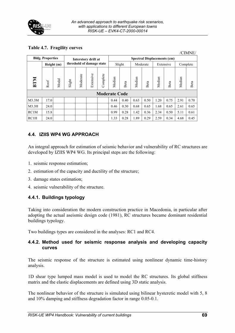
An advanced approach to earthquake risk scenarios,
with applications to different European towns RISK-UE – EVK4-CT-2000-00014
RISK-UE WP4 Handbook: Vulnerability of current buildings
69
Table 4.7. Fragility curves /CIMNE/
Bldg. Properties Spectral Displacements (cm)
Height (m) Interstory drift at
threshold of damage state Slight Moderate Extensive Complete
BT
M
Roo
f
Mod
al
Slig
ht
Mod
erat
e
Exte
nsiv
e
Com
plet
e
Med
ian
Bet
a
Med
ian
Bet
a
Med
ian
Bet
a
Med
ian
Bet
a
Moderate Code M3.3M 17.0 0.44 0.40 0.63 0.50 1.20 0.75 2.91 0.70
M3.3H 24.0 0.46 0.30 0.68 0.65 1.68 0.65 2.61 0.65
RC1M 15.8 0.99 0.28 1.42 0.36 2.34 0.50 5.11 0.61
RC1H 24.0 1.33 0.28 1.89 0.29 2.59 0.34 4.68 0.45
4.4. IZIIS WP4 WG APPROACH An integral approach for estimation of seismic behavior and vulnerability of RC structures are developed by IZIIS WP4 WG. Its principal steps are the following: 1. seismic response estimation;
2. estimation of the capacity and ductility of the structure;
3. damage states estimation;
4. seismic vulnerability of the structure.
4.4.1. Buildings typology Taking into consideration the modern construction practice in Macedonia, in particular after adopting the actual aseismic design code (1981), RC structures became dominant residential buildings typology. Two buildings types are considered in the analyses: RC1 and RC4.
4.4.2. Method used for seismic response analysis and developing capacity curves
The seismic response of the structure is estimated using nonlinear dynamic time-history analysis. 1D shear type lumped mass model is used to model the RC structures. Its global stiffness matrix and the elastic displacements are defined using 3D static analysis. The nonlinear behavior of the structure is simulated using bilinear hysteretic model with 5, 8 and 10% damping and stiffness degradation factor in range 0.05-0.1.

An advanced approach to earthquake risk scenarios,
with applications to different European towns RISK-UE – EVK4-CT-2000-00014
RISK-UE WP4 Handbook: Vulnerability of current buildings
70
Representative set of earthquakes is defined to cover wide amplitude/frequency characteristics of possible future events. Seismic hazard dissagregation techniques are emphasized to estimate the possible hazard-consistent magnitude-distance-predominant period parameters to be used in deciding the representative the time histories from existing earthquake data bases or artificial earthquake generation. An extensive strong motion database from 1979 Montenegro earthquake is used to develop the representative set of earthquake records. Some world-wide earthquake records as well as local strong motion data from 1994 Bitola Earthquake are also included in the stated set. The capacity of the structure is defined by diagram of dynamic capacity that is approximated by bilinear capacity curve using regression analysis. Every point of the diagram of dynamic capacity represents seismic response of the structure for certain PGA and earthquake record. Capacity curves and corresponding capacity spectra are developed for RC1 and RC4 buildings. In order to define the representative capacity spectra for the stated building types an extensive building data base consisted of 52 RC buildings with different structural characteristics is considered.
4.4.3. Definition of damage states Five damage states are adopted in IZIIS method. These damage states are correlated with 1985, Park&Ang Damage index (Table 4.8) as follows Table 4.8. Park and Ang damage index
Damage grade Definition Damage index (DI) range 0 No damage < 0.10 1 Slight damage 0.10-0.25 2 Moderate damage 0.25-0.40 3 Extensive damage 0.40-1.00 4 Collapse > 1.00
4.4.4. Fragility models and damage probability matrices The following procedure is used to develop the fragility curves: 1. Global damage indices are correlated with the corresponding spectral displacements at the
top of the equivalent SDOF system; 2. Normal standard distribution is adopted to model the damage index and its variability for
discretized spectral displacement space (discretization step 0.5-1.0 cm). Corresponding mean value of the damage index (DIav) and the standard deviation σDI are calculated (Fig. 4.2).

An advanced approach to earthquake risk scenarios,
with applications to different European towns RISK-UE – EVK4-CT-2000-00014
RISK-UE WP4 Handbook: Vulnerability of current buildings
71
3. Estimation of the conditional probability [ ]KDIDIP ≥ to reach or exceed certain damage states defined by damage indices DIk (Table 4.8)
[ ]
σ−
Φ−=≥DI
avKK
DIDI1DIDIP (4-2)
4. The parameters of the fragility curves i.e., the median value of the spectral displacement
and the corresponding lognormal standard deviation are estimated using regression analysis of the discrete values [ ]KDIDIP ≥ and the average value of the spectral displacement ranges.
The damage probability matrices are modeled with doubly bounded normalized normal standard distribution as follows (Eq 4-3)
[ ]
σ−
Φ−
σ−
Φ
σ−
Φ−
σ
−Φ
=
+
DI
av1
DI
avn
DI
avK
DI
av1K
DIDIDIDI
DIDIDIDI
dsP (4-3)
ds is damage state, DIk is the global damage index for damage state k; DIn >> 1.0 and DI1 = 0.0.
0
0.2
0.4
0.6
0.8
1
1.2
1.4
1.6
1.8
2
0 5 10 15 20 25
SD
DI
0
0.5
1
1.5
2
2.5
3
3.5
4
4.5
0 0.2 0.4 0.6 0.8 1 1.2 1.4 1.6
DIavσDI
Fig. 4.2. Correlation of Sd and DI
The capacity and fragility curves developed by IZIIS WP4 WG are presented in the Tables 4.9 and 4.10.
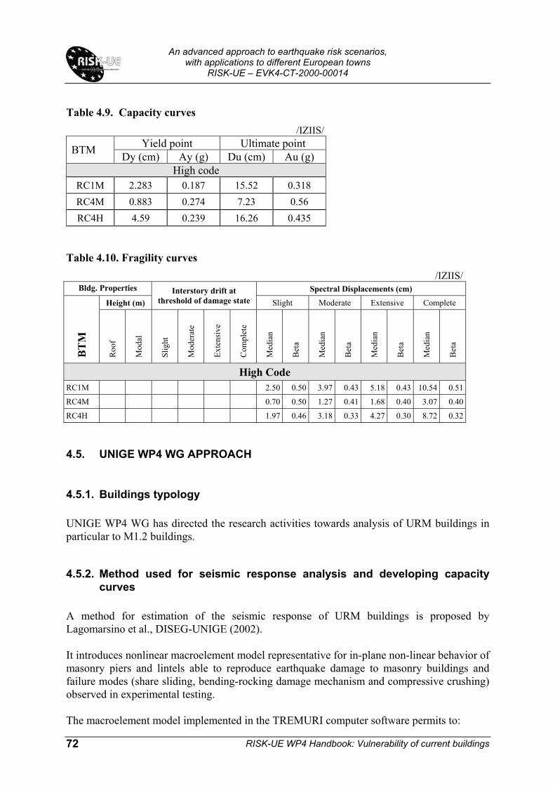
An advanced approach to earthquake risk scenarios,
with applications to different European towns RISK-UE – EVK4-CT-2000-00014
RISK-UE WP4 Handbook: Vulnerability of current buildings
72
Table 4.9. Capacity curves /IZIIS/
Yield point Ultimate point BTM Dy (cm) Ay (g) Du (cm) Au (g) High code
RC1M 2.283 0.187 15.52 0.318 RC4M 0.883 0.274 7.23 0.56 RC4H 4.59 0.239 16.26 0.435
Table 4.10. Fragility curves /IZIIS/
Bldg. Properties Spectral Displacements (cm)
Height (m) Interstory drift at
threshold of damage state Slight Moderate Extensive Complete
BT
M
Roo
f
Mod
al
Slig
ht
Mod
erat
e
Exte
nsiv
e
Com
plet
e
Med
ian
Bet
a
Med
ian
Bet
a
Med
ian
Bet
a
Med
ian
Bet
a
High Code RC1M 2.50 0.50 3.97 0.43 5.18 0.43 10.54 0.51
RC4M 0.70 0.50 1.27 0.41 1.68 0.40 3.07 0.40
RC4H 1.97 0.46 3.18 0.33 4.27 0.30 8.72 0.32
4.5. UNIGE WP4 WG APPROACH
4.5.1. Buildings typology UNIGE WP4 WG has directed the research activities towards analysis of URM buildings in particular to M1.2 buildings.
4.5.2. Method used for seismic response analysis and developing capacity curves
A method for estimation of the seismic response of URM buildings is proposed by Lagomarsino et al., DISEG-UNIGE (2002). It introduces nonlinear macroelement model representative for in-plane non-linear behavior of masonry piers and lintels able to reproduce earthquake damage to masonry buildings and failure modes (share sliding, bending-rocking damage mechanism and compressive crushing) observed in experimental testing. The macroelement model implemented in the TREMURI computer software permits to:
An advanced approach to earthquake risk scenarios,
with applications to different European towns RISK-UE – EVK4-CT-2000-00014
RISK-UE WP4 Handbook: Vulnerability of current buildings
73
• obtain Capacity Curves by 3D pushover analyses;
• evaluate the equivalent hysteretic damping, corresponding to different levels of horizontal displacement;
• detect damage limit states considering global and local damage parameters;
• perform non-linear step-by-step dynamic analyses, in order to validate the simplified method results.
The effectiveness and reliability of the TREMURI program is verified on a full scale model of masonry building, experimentally tested to the collapse in the laboratory of the University of Pavia [Magenes et al., 1997]. The pushover curve is converted into capacity spectrum
roof,dS S β= (4-4) where β = hload / hroof is the ratio between the height of the horizontal resulting force of the applied load vector hload assumed as the height of the equivalent SDOF system, and hroof the roof height. The base-shear is converted into horizontal acceleration by imposing the tangency condition of the linear branch of the curve with the constant period (T = T1) line in the origin of the axes. The base-shear V is divided by the equivalent mass value meq obtained from (Eq 4-5)
eroofd,
2
21
e
eqS 4
T Vm
βπ= (4-5)
where Ve is a value of the base shear in the elastic branch of the pushover curve and e
roofd,S is the corresponding roof displacement.
4.5.3. Fragility models For developing fragility models the following procedure is proposed: 1. Definition of bilinear capacity spectra with the following AD coordinates: yielding point
(Dy, Ay) and ultimate point (Du, Au) 2. definition of damage threshold spectral displacements (Eq 4-6)
( )DuSd
DyDu25.0DySdDySd
Dy7.0Sd
4
3
2
1
=−+=
==
(4-6)
An advanced approach to earthquake risk scenarios,
with applications to different European towns RISK-UE – EVK4-CT-2000-00014
RISK-UE WP4 Handbook: Vulnerability of current buildings
74
3. definition of lognormal standard deviation as a function of ultimate ductility µu (Eq 4-7)
( )u1 ln07.025.0 µ+=β ( )u2 ln18.02.0 µ+=β (4-7)
( )u3 ln4.01.0 µ+=β ( )u4 ln5.015.0 µ+=β The capacity and fragility curves developed by UNIGE WP4 WG are presented in the Tables 4.11 and 4.12.
Table 4.11. Capacity curves /UNIGE/
Yield point Ultimate point BTM
Dy (cm) Ay (g) Du (cm) Au (g) Pre code
M1.1L 0.38 0.173 1.93 0.173 M1.1M 0.47 0.115 2.03 0.115 M1.1H 0.66 0.058 2.28 0.058 M1.2L 0.15 0.15 1.55 0.15 M1.2M 0.31 0.12 1.69 0.132 M1.2H 0.48 0.10 1.85 0.12 M3.4L 0.53 0.297 3.18 0.297 M3.4M 0.75 0.149 3.47 0.149 M3.4H 0.92 0.099 3.67 0.099 RC1L 0.77 0.187 4.47 0.187 RC1M 2.21 0.156 8.79 0.156 RC1H 3.86 0.073 11.48 0.073
Moderate code RC1L 1.52 0.375 8.94 0.375 RC1M 4.42 0.312 17.55 0.312 RC1H 7.70 0.147 22.99 0.147
Table 4.12. Fragility curves /UNIGE/
Bldg. Properties Spectral Displacements (cm)
Height (m) Interstory drift at
threshold of damage state Slight Moderate Extensive Complete
BT
M
Roo
f
Mod
al
Slig
ht
Mod
erat
e
Exte
nsiv
e
Com
plet
e
Med
ian
Bet
a
Med
ian
Bet
a
Med
ian
Bet
a
Med
ian
Bet
a
Pre Code M1.2L 0.15 0.36 0.71 1.55
M1.2M 0.31 0.51 0.86 1.69
M1.2H 0.48 0.69 1.03 1.85

An advanced approach to earthquake risk scenarios,
with applications to different European towns RISK-UE – EVK4-CT-2000-00014
RISK-UE WP4 Handbook: Vulnerability of current buildings
75
4.6. UTCB WP4 WG APPROACH UTCB WP4 WG proposed an analytical approach that uses Monte Carlo simulation technique to obtain parameters of the capacity and fragility models.
4.6.1. Buildings typology Capacity and fragility models are developed for representative RC1H (low and moderate code) as well as RC2M (moderate code) and RC2H (low code) buildings.
4.6.2. Method used for seismic response analysis and developing capacity curves
Pushover analysis is used to estimate the seismic response of buildings and to develop capacity curves. The Monte-Carlo technique as applied to select the values of the input capacity random variables required for pushover analyses. The Latin hypercube to perform stratified sampling of the input variables and to reduce the number of samples by significant decrease in the variance of estimators. In brief, the simulation technique implies the following steps: • simulation of structural parameters;
• random permutations of structural random variables;
• performing push-over analyses using generated samples;
• sample statistics of the results of analyses. Normal probability distribution for concrete strength and a lognormal probability distribution for steel strength might are used (Galambos et al. 1982). The outcome of the pushover analyses is a family of capacity curves, which can be described as mean or mean plus/minus one standard deviation capacity curves.
4.6.3. Damage states Five damage states are adopted in UTCB method. These damage states are correlated with 1985, Park&Ang Damage index (Table 4.8)
4.6.4. Fragility models Fragility models are developed using the following approach: 1. Determine the correlation between Park&Ang damage index and interstory drift as mean
and standard deviation values.

An advanced approach to earthquake risk scenarios,
with applications to different European towns RISK-UE – EVK4-CT-2000-00014
RISK-UE WP4 Handbook: Vulnerability of current buildings
76
2. Identify the mean and standard deviation values of interstory drift at threshold of damage state (Fig. 4.3)
13 stories
0.0
0.5
1.0
1.5
2.0
2.5
3.0
3.5
4.0
4.5
5.0
0.0 0.2 0.4 0.6 0.8 1.0 1.2 1.4 1.6 1.8 2.0
Park&Ang Damage Index
Dri
ft Ra
tio, %
µµ−σµ+σ
Fig. 4.3. Correlation of DI and Drift Ratio
3. The median value of spectral displacement at which the building reaches the threshold of
the damage state, Sd,ds is obtained by multiplying the interstory drift by the height of the building and by the fraction of the building height at the location of push-over mode displacement.
The total variability of each structural damage state, βSds, is modeled by the combination of three contributors to structural damage variability, βC, βD and βM(Sds), as follows (Eq 4-8)
( )2)Sds(M
2D
2CSds β+β+β=β (4-8)
βSds is the lognormal standard deviation that describes the total variability for structural
damage state, ds,
βC is the lognormal standard deviation parameter that describes the variability of the capacity curve,
βD is the lognormal standard deviation parameter that describes the variability of the demand spectrum,
βM(Sds) is the lognormal standard deviation parameter that describes the uncertainty in the estimate of the median value of the threshold of structural damage state, ds.
The capacity and fragility curves developed by UTCB WP4 WG are presented in the Tables 4.13 and 4.14.

An advanced approach to earthquake risk scenarios,
with applications to different European towns RISK-UE – EVK4-CT-2000-00014
RISK-UE WP4 Handbook: Vulnerability of current buildings
77
Table 4.13. Capacity curves /UTCB/
Yield point Ultimate point BTM Dy (cm) Ay (g) Du (cm) Au (g) Low code
RC1H 10.3 0.068 99.0 0.070 RC2H 1.3 0.215 7.4 0.302
Moderate code RC1H 6.2 0.138 89.0 0.20 RC2M 1.8 0.32 6.0 0.34
Table 4.14. Fragility curves /UTCB/
Bldg. Properties Spectral Displacements (cm)
Height (m) Interstory drift at
threshold of damage state Slight Moderate Extensive Complete
BT
M
Roo
f
Mod
al
Slig
ht
Mod
erat
e
Exte
nsiv
e
Com
plet
e
Med
ian
Bet
a
Med
ian
Bet
a
Med
ian
Bet
a
Med
ian
Bet
a
Low Code RC1H 37.97 27.94 0.00 0.01 0.01 0.02 7.82 0.65 17.88 0.75 27.94 0.85 68.16 0.95
RC2H 31.00 21.99 0.02 0.06 0.09 0.24 0.52 0.65 1.30 0.75 2.09 0.85 5.22 0.95
Moderate Code RC1H 30.80 24.84 0.00 0.01 0.01 0.03 11.67 0.65 21.61 0.75 31.79 0.85 72.03 0.95
RC2M 22.00 16.19 0.00 0.00 0.00 0.00 0.46 0.65 1.02 0.75 1.58 0.85 3.84 0.95
4.7. CODE BASED APPROACH (CBA) A hybrid method for development of capacity curves and fragility functions is elaborated (hereafter noted as CBA method). The CBA method is performed as follows: 1. The capacity spectra are modeled as bilinear curves in AD format (Eq 4-9)
YC (Ay, Dy) 1
sy
CA
αγ
= 22y
y T4
AD
π= (4-9)
UC (Au, Du) 1
syu
CAA
αγ
λ=λ= 2
2
1
syu
4TC
DDπα
γλµ=λµ=

An advanced approach to earthquake risk scenarios,
with applications to different European towns RISK-UE – EVK4-CT-2000-00014
RISK-UE WP4 Handbook: Vulnerability of current buildings
78
Cs design strength coefficient (fraction of building’s weight),
T true “elastic” fundamental-mode period of building (seconds),
α1 fraction of building weight effective in push-over mode,
γ “overstrength” factor relating “true” yield strength to design strength,
λ “overstrength” factor relating ultimate strength to yield strength, and
µ “ductility” factor relating ultimate displacement to λ times the yield displacement (i.e., assumed point of significant yielding of the structure)
The design strength, Cs is based on the lateral-force design requirements of the seismic codes. It is a function of the seismic zone and other factors including site soil conditions, the type of lateral-force-resisting system and building period. The coefficient α1 is defined with the buildings modal characteristics as follows (Eq 4-10)
[ ]∑ ∑
∑φ
φ=α 2
iii
2ii
1mm
m mi - story masses; φi - modal shapes (4-10)
The overstrength (γ, λ) and ductility (µ) parameters are defined by the code requirements as well as experimental data and expert judgment. 2. The fragility curves are modeled by lognormal standard distribution; To obtain discrete damage states, the Park & Ang damage index is adopted (Table 4.8): The median values of the spectral displacements pertinent to certain damage state are determined using the following equations (Eq 4-11)
( )uy
yye
yu
y
DAADDAk4
DDDD
DI−
β+−
−= ( )y
yu
yuy DD
DDAA
AA −−
−+= (4-11)
where D is median value of the spectral displacement at certain damage state and k is degradation factor that defines the effective amount of hysteretic damping. Variability of the spectral displacements are obtained using different procedures proposed by: IZIIS, UTCB, UNIGE. The capacity and fragility curves developed by IZIIS and UTCB WP4 WG are presented in the Tables 4.15 and 4.16.

An advanced approach to earthquake risk scenarios,
with applications to different European towns RISK-UE – EVK4-CT-2000-00014
RISK-UE WP4 Handbook: Vulnerability of current buildings
79
Table 4.15. Capacity curves /IZIIS, UTCB/
Yield point Ultimate point BTM Institution Dy (cm) Ay (g) Du (cm) Au (g) Pre Code
RC1M UTCB 1.00 0.082 3.01 0.124 RC1H UTCB 2.32 0.093 6.96 0.140 RC2M UTCB 0.31 0.078 0.93 0.117 RC2H UTCB 1.07 0.088 3.20 0.131
Low Code RC1M UTCB 0.64 0.053 2.90 0.079 RC1H UTCB 1.04 0.042 4.70 0.063 RC2M UTCB 0.48 0.12 2.15 0.180 RC2H UTCB 0.88 0.073 3.98 0.109
Moderate Code RC1L IZIIS 0.10 0.18 0.22 0.20
IZIIS 1.51 0.17 3.31 0.19 UTCB-1 0.68 0.056 3.07 0.084 RC1M UTCB-2 1.26 0.141 12.63 0.282 IZIIS 3.52 0.10 7.75 0.11 UTCB-1 1.11 0.045 5.01 0.067 RC1H UTCB-2 2.87 0.160 28.73 0.320 UTCB-1 0.45 0.112 2.00 0.168 RC2M UTCB-2 0.51 0.167 4.06 0.333 UTCB-1 0.94 0.077 4.22 0.116 RC2H UTCB-2 1.68 0.188 13.42 0.375
High Code RC1L IZIIS 0.07 0.13 0.59 0.26
IZIIS 1.31 0.15 10.44 0.29 RC1M UTCB 1.58 0.176 15.79 0.353 IZIIS 4.58 0.13 36.63 0.26 RC1H UTCB 3.59 0.200 35.91 0.400
RC2M UTCB 0.63 0.208 5.07 0.417 RC2H UTCB 2.10 0.234 16.77 0.469

An advanced approach to earthquake risk scenarios,
with applications to different European towns RISK-UE – EVK4-CT-2000-00014
RISK-UE WP4 Handbook: Vulnerability of current buildings
80
Table 4.16. Fragility Curves /IZIIS, UTCB/
Bldg. Properties Spectral Displacements (cm)
Height (m) Interstory drift at
threshold of damage state Slight Moderate Extensive Complete
BT
M
Inst
itutio
n
Roo
f
Mod
al
Slig
ht
Mod
erat
e
Exte
nsiv
e
Com
plet
e
Med
ian
Bet
a
Med
ian
Bet
a
Med
ian
Bet
a
Med
ian
Bet
a
Pre Code RC1L 5 570 342 0.04 0.08 0.13 0.30 0.14 0.65 0.29 0.75 0.44 0.85 1.03 0.95RC1M 5 1710 1026 0.04 0.08 0.12 0.27 0.38 0.65 0.78 0.75 1.18 0.85 2.79 0.95RC1H 5 2850 1710 0.05 0.11 0.16 0.38 0.87 0.65 1.80 0.75 2.73 0.85 6.46 0.95RC2L 5 570 399 0.00 0.01 0.01 0.03 0.01 0.65 0.03 0.75 0.05 0.85 0.11 0.95RC2M 5 1710 1197 0.01 0.02 0.03 0.07 0.12 0.65 0.24 0.75 0.36 0.85 0.86 0.95RC2H 5 2850 1995 0.02 0.04 0.06 0.15 0.40 0.65 0.83 0.75 1.26 0.85 2.97 0.95
Low Code RC1L 5 570 342 0.06 0.12 0.18 0.43 0.20 0.65 0.41 0.75 0.62 0.85 1.47 0.95RC1M 5 1710 1026 0.03 0.07 0.11 0.25 0.34 0.65 0.71 0.75 1.08 0.85 2.55 0.95RC1H 5 2850 1710 0.03 0.07 0.10 0.24 0.56 0.65 1.15 0.75 1.75 0.85 4.14 0.95RC2L 5 570 399 0.01 0.02 0.03 0.07 0.04 0.65 0.08 0.75 0.12 0.85 0.28 0.95RC2M 5 1710 1197 0.02 0.04 0.07 0.16 0.25 0.65 0.53 0.75 0.80 0.85 1.89 0.95RC2H 5 2850 1995 0.02 0.05 0.07 0.18 0.47 0.65 0.98 0.75 1.48 0.85 3.51 0.95
Moderate Code 3 0.11 0.40 0.13 0.50 0.15 0.60 0.21 0.70
5A 570 342 0.06 0.13 0.19 0.46 0.21 0.65 0.43 0.75 0.66 0.85 1.56 0.95RC1L 5B 570 342 0.15 0.32 0.50 1.21 0.50 0.65 1.11 0.75 1.72 0.85 4.15 0.953 1.67 0.40 1.92 0.50 2.17 0.60 3.16 0.70
5A 1710 1026 0.04 0.07 0.11 0.26 0.36 0.65 0.75 0.75 1.14 0.85 2.70 0.95RC1M 5B 1710 1026 0.12 0.27 0.42 1.02 1.26 0.65 2.79 0.75 4.32 0.85 10.43 0.953 3.91 0.40 4.49 0.50 5.07 0.60 7.40 0.70
5A 2850 1710 0.04 0.07 0.11 0.26 0.59 0.65 1.23 0.75 1.87 0.85 4.42 0.95RC1H 5B 2850 1710 0.17 0.37 0.57 1.39 2.87 0.65 6.35 0.75 9.82 0.85 23.72 0.955A 570 399 0.01 0.02 0.02 0.06 0.03 0.65 0.06 0.75 0.09 0.85 0.22 0.95
RC2L 5B 570 399 0.01 0.02 0.03 0.06 0.03 0.65 0.07 0.75 0.10 0.85 0.25 0.955A 1710 1197 0.02 0.04 0.06 0.15 0.24 0.65 0.49 0.75 0.75 0.85 1.77 0.95
RC2M 5B 1710 1197 0.04 0.08 0.12 0.28 0.43 0.65 0.92 0.75 1.41 0.85 3.37 0.955A 2850 1995 0.03 0.05 0.08 0.19 0.50 0.65 1.04 0.75 1.57 0.85 3.72 0.95
RC2H 5B 2850 1995 0.07 0.15 0.23 0.56 1.41 0.65 3.03 0.75 4.65 0.85 11.15 0.95
High Code 3 0.12 0.40 0.19 0.50 0.26 0.60 0.53 0.70
RC1L 5 570 342 0.18 0.39 0.59 1.40 0.63 0.65 1.32 0.75 2.01 0.85 4.78 0.953 2.11 0.40 3.31 0.50 4.52 0.60 9.35 0.70
RC1M 5 1710 1026 0.15 0.32 0.49 1.17 1.58 0.65 3.32 0.75 5.06 0.85 12.03 0.953 7.40 0.40 11.64 0.50 15.87 0.60 32.82 0.70
RC1H 5 2850 1710 0.21 0.44 0.67 1.60 3.59 0.65 7.55 0.75 11.51 0.85 27.35 0.95
RC2L 5 570 399 0.01 0.02 0.03 0.07 0.04 0.65 0.08 0.75 0.12 0.85 0.29 0.95RC2M 5 1710 1197 0.05 0.09 0.14 0.33 0.54 0.65 1.10 0.75 1.66 0.85 3.90 0.95RC2H 5 2850 1995 0.09 0.18 0.28 0.65 1.79 0.65 3.64 0.75 5.49 0.85 12.89 0.95
Institutions: 1-AUTH; 2-CIMNE; 3-IZIIS; 4-UNIGE; 5-UTCB (5A 1970-77; 5B 1978-89)
An advanced approach to earthquake risk scenarios,
with applications to different European towns RISK-UE – EVK4-CT-2000-00014
RISK-UE WP4 Handbook: Vulnerability of current buildings
81
5. References 1. ATC (1985). Earthquake damage evaluation data for California (ATC-13). Appl.
Technology Council, Redwood City, Calif.
2. ATC 40. Seismic evaluation and retrofit of concrete buildings, Vol. 1, ATC, Report SSC 96-01.
3. ATC 40. Seismic Evaluation and Retrofit of Concrete Buildings, Report ATC-40, Applied Technology Council, Redwood City CA., 1996
4. Barbat A.H. et al. (1996). Damage Scenarios Simulation for Seismic Risk Assessment in Urban Zones, Earthquake Spectra, 12(3), 371-394.
5. Benedetti D., P. Carydis and P. Pezzoli (1998). Shaking table tests on 24 simple masonry buildings, Earthquake Engineering & Structural Dynamics, 27(1), 67-90.
6. Braga F., M. Dolce and D. Liberatore (1982). Southern Italy November 23, 1980 Earthquake: A Statistical Study on Damaged Buildings and an Ensuing Review of the M.S.K.-76 Scale. CNR-PFG n.203, Roma.
7. Building Research Institute, Ministry of Construction, Japan, 1978. Digitized data of strong-motion earthquake accelerograms in Romania (March 4, 1977) by Observational Committee of Strong Motion Earthquake, Kenchiku Kenkyu Shiro No.20, January.
8. Calvi G.M., G.R. Kingsley and G. Magenes (1996). Testing of Masonry Structures for Seismic Assessment, Earthquake Spectra, 12 (1), 145-162.
9. Calvi G.M. (1999). A displacement-based approach for vulnerability evaluation of classes of buildings, Journal of Earthquake Engineering, 3(3), 411-438.
10. Chopra A.K. (1995). Dynamics of structures: theory and applications to earthquake engineering. Englewood Cliffs, N.J.: Prentice Hall.
11. Chopra A.K. and R.K. Goel (1999). Capacity-Demand-Diagram Methods For Estimating Seismic Deformation Of Inelastic Structures: SDF Systems, Report No. PEER-1999/02, Pacific Earthquake Engineering Research Center, 72 p.
12. Cornea T., R. Vacareanu and D. Lungu (2000). Technical Report for Collaborative Research Center (CRC) 461 of SFB, Germany: “Strong Earthquakes: A Challenge for Geosciences and Civil Engineering”, Karlsruhe University, 64 p.
13. Dolce M., A. Kappos, G. Zuccaro and A.W. Coburn (1995). State of the Art Report of W.G. 3 - Seismic Risk and Vulnerability, 10th European Conference on Earthquake Engineering, Vienna, Austria (Aug. - Sep. 1994), Vol. 4, 3049-3077.
14. Dolce, M., Marino, M., Masi, A. and Vona, M. (2000) Seismic vulnerability analysis and damage scenarios of Potenza, International Workshop on Seismic Risk and Earthquake Scenarios of Potenza (Potenza, Italy, Nov. 2000).
15. Fajfar P. and H. Krawlinker, ed. (1997). Seismic design methodologies for the next generation of codes, Proceedings of the International Workshop, Bled, Slovenia, June 24-27, 1997, Balkema Rotterdam, ISBN 90 5410 928 9.
16. Fajfar P. and M. Dolsek (2003). Extension of the Non-linear Method of Simplified Non-linear seismic analysis to Infilled RC Frames, SE40EEE, Ohrid, 2003.

An advanced approach to earthquake risk scenarios,
with applications to different European towns RISK-UE – EVK4-CT-2000-00014
RISK-UE WP4 Handbook: Vulnerability of current buildings
82
17. Fajfar P. (2002). Structural Analysis in Earthquake Engineering - A Breaktrough of Simplified Non-linear Methods. 12th European Conference on Earthquake Engineering, London, 2002.
18. Fardis M.N., F.V. Karantoni and A. Kosmopoulos (1999). Statistical evaluation of damage during the 15-6-95 Aegio Earthquake, Final Report to the Sponsor (EPPO, Athens), Patras (in Greek).
19. FEMA (1997). NEHRP Guidelines for the Seismic Rehabilitation of Buildings, FEMA-273, Washington D.C., Oct. 1997.
20. FEMA/NIBS, HAZUS - Earthquake Loss Estimation Methodology, Vol. 1, 1998.
21. Fishinger M., T. Isakovic and P. Kante (2003). Application of Simplified Nonlinear - N2 Method for Some Common Types of RC Structures, SE40EEE, Ohrid, 2003.
22. Fishinger M., P. Fajfar, M. Dolsek, D. Zamfirescu, A. Stratan, T. Leino, R. Vacareanu, T. Cornea, D. Lungu, S. Wolinski and E. Alarcon. General Methodologies for Evaluating the Structural Performance under Exceptional Loadings.
23. Freeman S.A., J.P. Nicoletti, and J.V. Tyrell (1975). Evaluations of existing buildings for seismic risk - A case study of Puget Sound Naval Shipyard, Bremerton, Washington.
24. Galambos T.V., B. Ellingwood, J.G. McGregor and C.A. Cornell (1982). Probability based load criteria: Assessment of current design practice. Journal of Structural Di-vision, ASCE, vol. 108, No. ST5, pp. 959-977, 1982.
25. HAZUS – Technical Manual 1997. Earthquake Loss Estimation Methodology, 3 Vol.
26. Kappos A.J., K.C. Stylianidis and K. Pitilakis (1998). Development of seismic risk scenarios based on a hybrid method of vulnerability assessment. Natural Hazards, 17(2): 177-192.
27. Kappos A.J. (2001). Seismic vulnerability assessment of existing buildings in Southern Europe, Keynote lecture, Convegno Nazionale “L’Ingegneria Sismica in Italia” (Potenza/Matera, Italy), CD ROM Proceedings.
28. Kappos A.J., K.D. Pitilakis, K. Morfidis and N. Hatzinikolaou (2002). Vulnerability and risk study of Volos (Greece) metropolitan area, 12th European Conference on Earthquake Engineering (London, Sep. 2002), CD ROM Proceedings (Balkema), Paper 074.
29. Kappos A.J., Gr.G. Penelis and C. Drakopoulos (2002). Evaluation of simplified models for the analysis of unreinforced masonry (URM) buildings, Journal of Structural Engineering, ASCE, Vol. 128, No. 7, 890-897.
30. Karantoni F.V. and G. Bouckovalas (1997). Description and analysis of building damage due to Pyrgos, Greece earthquake, Soil Dynamics & Earthquake Engineering, 16(2), 141-150.
31. Kappos A.J. (2001). Seismic Vulnerability Assessment of Existing Buildings in Southern Europe, ANIDIS 2001.
32. Kappos A.J. and E. Papadopoulos (2000). Seismic Vulnerability Assessment of the Potenza Building Stock Using the Greek Methodology, Potenza, 2000.

An advanced approach to earthquake risk scenarios,
with applications to different European towns RISK-UE – EVK4-CT-2000-00014
RISK-UE WP4 Handbook: Vulnerability of current buildings
83
33. Kappos A.J., Ch. Panagiotopoulos and E. Papadopoulos (2003). WP4 - 1st and 2nd Level Analysis: Reinforced Concrete Buildings, Thessaloniki, 2003.
34. Lekidis V.A. et al. (1999). The Aegio (Greece) seismic sequence of June 1995: Seismological, strong motion data and effects of the earthquakes on structures, Journal of Earthquake Engineering, 3(3), 349-380.
35. Lekkas E., I. Fountoulis and D. Papanikolaou (2000). Intensity Distribution and Neotectonic Macrostructure Pyrgos Earthquake Data (26 March 1993, Greece), Natural Hazards 21(1): 19–33.
36. Magenes G. and G.M. Calvi (1997). In-plane seismic response of brick masonry walls, Earthquake Engineering and Structural Dynamics, 26(11), 1091-1112.
37. Milutinovic Z. and H. Kameda (1984). Statistical model for estimation of inelastic response spectra. Proc. of JSCE Struc. Eng. / Earthq. Eng Vol. 1, No. 2, October 1984.
38. Milutinovic Z.V. and G.S. Trendafiloski (2001). Prevalent building typology in the city of Bitola, RISK-UE WP1, Objective 2 Report, IZIIS-Skopje, October 2001.
39. Milutinovic Z.V. and G.S. Trendafiloski (2002). WP4: Level 2 methodology - Code based approach, Case study: Aseismic Design Codes in Macedonia, RISK-UE WP4 L2 Report, IZIIS, Skopje.
40. Moreno R., N. Lantada, R. Bonett, A.H. Barbat and L.G. Pujades (2003). WP4: Vulnerability Assesment of Current Buildings. Capacity and Fragility of the Barcelona's Residential Buildings, Report by CIMNE Working Group, 2003.
41. Newmark N.M. and W.J. Hall (1982). Earthquake Spectra and Design. Berkeley, Calif. Earthquake Engineering Research Inst.
42. Official Gazette of F.P.R. Yugoslavia, No. 61/48.
43. Official Gazette of S.F.R. Yugoslavia, No. 39/64.
44. Official Gazette of S.F.R. Yugoslavia, No. 31/81, 49/82, 29/83, 21/88, 52/90.
45. Official Gazette of S.F.R. Yugoslavia, No. 52/85.
46. Papazachos B. and C. Papazachou (1997). The Earthquakes of Greece, Ziti Editions, Thessaloniki.
47. Park Y.J. and A.H. Ang (1985). Mechanistic seismic damage model for reinforced concrete. Journal of Structural Engineering. ASCE vol. 111 (4): 722-739, 1985.
48. Penelis G.G., D. Sarigiannis, E. Stavrakakis and K.C. Stylianidis (1989). A statistical evaluation of damage to buildings in the Thessaloniki, Greece, earthquake of June, 20, 1978. Proceedings of 9th World Conf. on Earthq. Eng., (Tokyo-Kyoto, Japan, Aug. 1988), Tokyo: Maruzen, VII: 187-192.
49. Penelis Gr.G., A.J. Kappos and K.C. Stylianidis (2002). WP4 – 1st level analysis: Unreinforced masonry buildings, RISK-UE document, May.
50. Penelis Gr.G, A.J. Kappos, K.C. Stylianidis and S. Lagomarsino. Statistical Assessment of the Vulnerability of Unreinforced Masonry Buildings.
51. Penelis Gr.G., A.J. Kappos, K.C. Stylianidis and Ch. Panagiotopoulos. 2nd Level Analysis and Vulnerability Assessment of URM Buildings.
An advanced approach to earthquake risk scenarios,
with applications to different European towns RISK-UE – EVK4-CT-2000-00014
RISK-UE WP4 Handbook: Vulnerability of current buildings
84
52. Proceedings of 1st U.S. National Conference on Earthquake Engineering, 113-22. Berkeley, Calif., EERI.
53. Rubinstein R. Y. (1981). Simulation and the Monte-Carlo method. John Wiley & Sons, New York, 1981.
54. Sandi H. (convener) - Vulnerability and Risk Analysis for Individual Structures and for Systems. Report of EAEE WG 5/10 to the 8-th European Conference on Earthquake Engineering, Lisbon, 1986.
55. Singhal A. and A.S Kiremidjian (1995). Method for Developing Motion Damage Relationships for Reinforced Concrete Frames, Technical Report NCEER-95-0008, May 1995.
56. Singhal A. and A.S. Kiremidjian (1997). A method for earthquake motion-damage relationships with application to reinforced concrete frames. Technical Report NCEER-97-0008. National Center for Earthquake Engineering Research, State University of New York at Buffalo.
57. Theodulidis N.P. and B.C. Papazachos (1992). Dependence of strong ground motion on magnitude-distance, site geology and macroseismic intensity for shallow earthquakes in Greece: Peak horizontal acceleration, velocity and displacement, Soil Dynamics and Earthquake Engineering, 11, 387-402.
58. Tomazevic M. and I. Klemenc (1997). Seismic behavior of confined masonry walls, Earthquake Engineering & Structural Dynamics, 26(10), 1059-71.
59. Trendafiloski G.S. and Z.V. Milutinovic (2003). GIS-oriented method for elaboration of probabilistic earthquake scenarios. Report IZIIS 2003-27, January 2003 (in Macedonian).
60. Văcăreanu R. (1998). Seismic Risk Analysis for a High Rise Building - Proceedings of the 11th European Conference on Earthquake Engineering, Paris, Abstract Volume pg. 513 and CD-ROM.
61. Văcăreanu R. (2000). Monte-Carlo Simulation Technique for Vulnerability Analysis of RC Frames - An Example - Scientific Bulletin on Technical University of Civil Engineering of Bucharest, pg. 9-18.
62. Văcăreanu R. and D. Lungu (2002). Capacity Curves and Fragility Functions for Representative Building Types in Bucharest, RISK-UE WP4 L2 Report, UTCB, Bucharest, Romania.
63. Văcăreanu R., T. Cornea, D. Lungu. Evaluation of seismic fragility of buildings, Earthquake Hazard and Countermeasures for Existing Fragile Buildings, Editors: Lungu D. & Saito T., Independent Film, Bucharest Romania.
64. Văcăreanu R., T. Cornea and D. Lungu. Assesment of Seismic Behavior and Fragility of buildings Using HAZUS and ATC-40 Methodologies.
65. Văcăreanu R. and D. Lungu Capacity and Fragility Curves for Representative Building Types in Bucharest
66. Valles R.E., A.M. Reinhorn, S.K. Kunnath, C. Li and A. Madan (1996). IDARC2D Version 4.0: A Computer Program for the Inelastic Damage Analysis of Buildings, Technical Report NCEER-96-0010, NCEER, State University of New York at Buffalo,

An advanced approach to earthquake risk scenarios,
with applications to different European towns RISK-UE – EVK4-CT-2000-00014
RISK-UE WP4 Handbook: Vulnerability of current buildings
85
1996.
67. Williams M.S. and R.G. Sexsmith (1995). Seismic Damage Indices for Concrete Structures: A State-of-the-Art Review. Earthquake Spectra. Vol. 11(2): 319-345, 1997.
68. WP4. Vulnerability Assessment of Current Buildings. Guidelines for the Implementation of the II Level Vulnerability Methodology (First Proposal for Masonry Buildings), 2002.

An advanced approach to earthquake risk scenarios,
with applications to different European towns RISK-UE – EVK4-CT-2000-00014
RISK-UE WP4 Handbook: Vulnerability of current buildings
86
Appendix A: Capacity models for masonry and RC buildings developed by different approaches and
partners
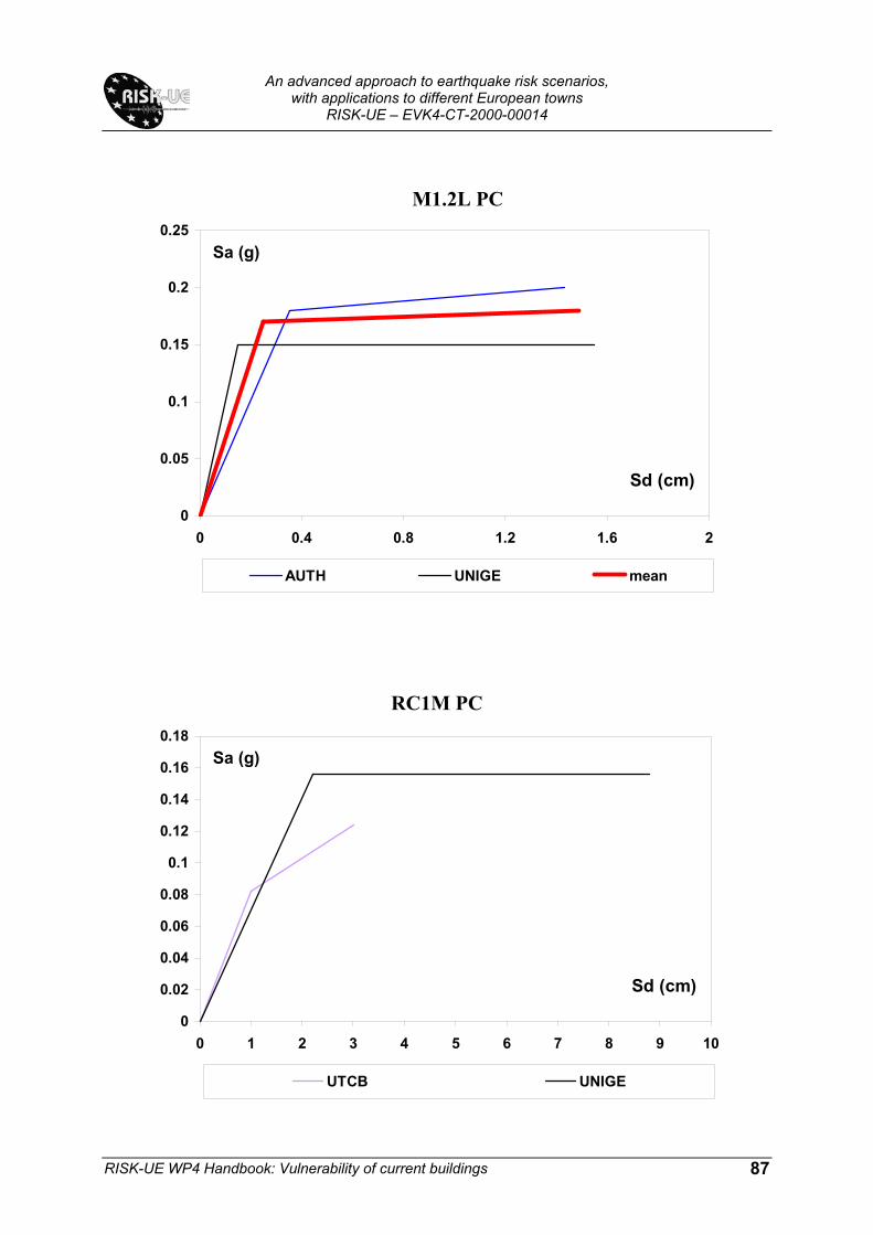
An advanced approach to earthquake risk scenarios,
with applications to different European towns RISK-UE – EVK4-CT-2000-00014
RISK-UE WP4 Handbook: Vulnerability of current buildings
87
M1.2L PC
0
0.05
0.1
0.15
0.2
0.25
0 0.4 0.8 1.2 1.6 2
Sd (cm)
Sa (g)
AUTH UNIGE mean
RC1M PC
0
0.02
0.04
0.06
0.08
0.1
0.12
0.14
0.16
0.18
0 1 2 3 4 5 6 7 8 9 10
Sd (cm)
Sa (g)
UTCB UNIGE

An advanced approach to earthquake risk scenarios,
with applications to different European towns RISK-UE – EVK4-CT-2000-00014
RISK-UE WP4 Handbook: Vulnerability of current buildings
88
RC1H PC
0
0.02
0.04
0.06
0.08
0.1
0.12
0.14
0.16
0 3 6 9 12 15
Sd (cm)
Sa (g)
UTCB UNIGE mean
RC1M LC
0
0.02
0.04
0.06
0.08
0.1
0.12
0.14
0.16
0.18
0.2
0 3 6 9 12 15
Sd (cm)
Sa (g)
UTCB AUTH

An advanced approach to earthquake risk scenarios,
with applications to different European towns RISK-UE – EVK4-CT-2000-00014
RISK-UE WP4 Handbook: Vulnerability of current buildings
89
RC1H LC
0
0.02
0.04
0.06
0.08
0.1
0.12
0.14
0.16
0 10 20 30 40 50 60 70 80 90 100
Sd (cm)
Sa (g)
AUTH UTCB UTCB-A HAZUS mean
RC2M LC
0
0.05
0.1
0.15
0.2
0.25
0.3
0 2 4 6 8 10
Sd (cm)
Sa (g)
AUTH UTCB HAZUS mean
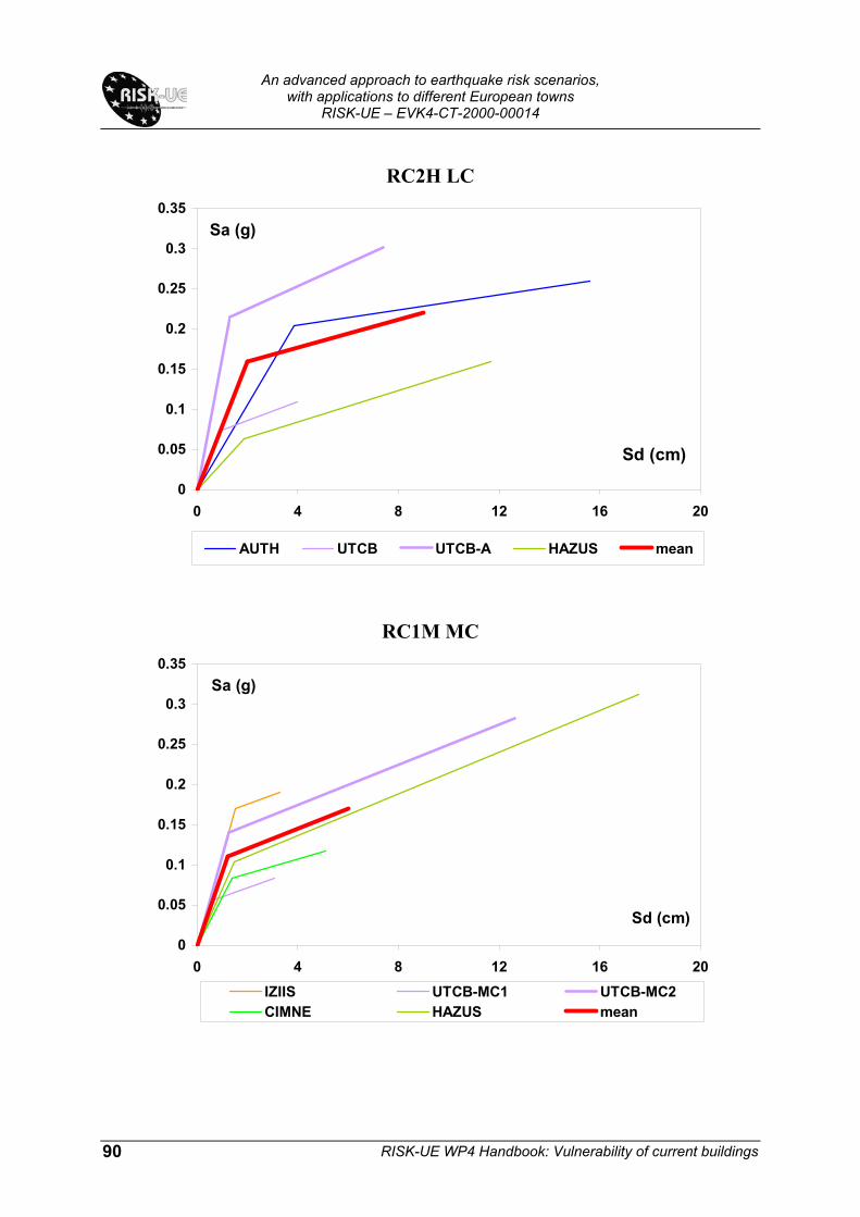
An advanced approach to earthquake risk scenarios,
with applications to different European towns RISK-UE – EVK4-CT-2000-00014
RISK-UE WP4 Handbook: Vulnerability of current buildings
90
RC2H LC
0
0.05
0.1
0.15
0.2
0.25
0.3
0.35
0 4 8 12 16 20
Sd (cm)
Sa (g)
AUTH UTCB UTCB-A HAZUS mean
RC1M MC
0
0.05
0.1
0.15
0.2
0.25
0.3
0.35
0 4 8 12 16 20
Sd (cm)
Sa (g)
IZIIS UTCB-MC1 UTCB-MC2CIMNE HAZUS mean

An advanced approach to earthquake risk scenarios,
with applications to different European towns RISK-UE – EVK4-CT-2000-00014
RISK-UE WP4 Handbook: Vulnerability of current buildings
91
RC1H MC
0
0.05
0.1
0.15
0.2
0.25
0.3
0.35
0 10 20 30 40 50 60
Sd (cm)
Sa (g)
IZIIS UTCB-MC1 UTCB-MC2 UTCB-MC-AUNIGE HAZUS CIMNE mean
RC2M MC
0
0.05
0.1
0.15
0.2
0.25
0.3
0.35
0.4
0.45
0 3 6 9 12 15
Sd (cm)
Sa (g)
UTCB-MC1 UTCB-MC2 UTCB-A HAZUS mean
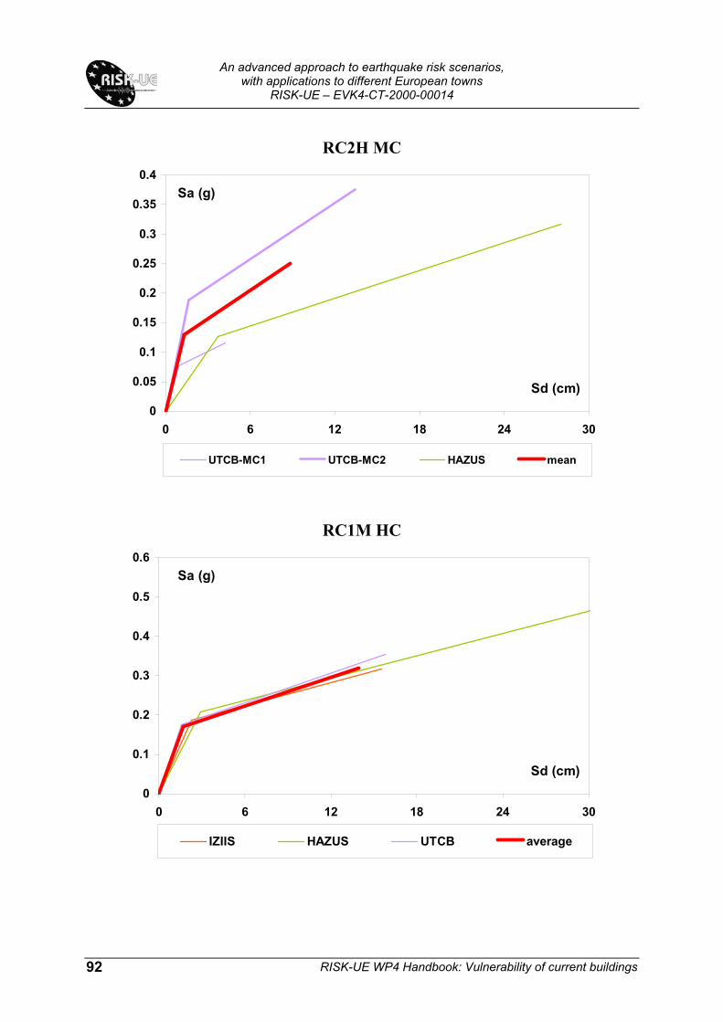
An advanced approach to earthquake risk scenarios,
with applications to different European towns RISK-UE – EVK4-CT-2000-00014
RISK-UE WP4 Handbook: Vulnerability of current buildings
92
RC2H MC
0
0.05
0.1
0.15
0.2
0.25
0.3
0.35
0.4
0 6 12 18 24 30
Sd (cm)
Sa (g)
UTCB-MC1 UTCB-MC2 HAZUS mean
RC1M HC
0
0.1
0.2
0.3
0.4
0.5
0.6
0 6 12 18 24 30
Sd (cm)
Sa (g)
IZIIS HAZUS UTCB average

An advanced approach to earthquake risk scenarios,
with applications to different European towns RISK-UE – EVK4-CT-2000-00014
RISK-UE WP4 Handbook: Vulnerability of current buildings
93
RC1H HC
0
0.05
0.1
0.15
0.2
0.25
0.3
0.35
0.4
0.45
0 10 20 30 40 50
Sd (cm)
Sa (g)
IZIIS UTCB HAZUS mean
RC1M HC
0
0.1
0.2
0.3
0.4
0.5
0.6
0 6 12 18 24 30
Sd (cm)
Sa (g)
AUTH UTCB HAZUS mean

An advanced approach to earthquake risk scenarios,
with applications to different European towns RISK-UE – EVK4-CT-2000-00014
RISK-UE WP4 Handbook: Vulnerability of current buildings
94
RC4M HC
0
0.1
0.2
0.3
0.4
0.5
0.6
0 2 4 6 8 10
Sd (cm)
Sa (g)
IZIIS AUTH mean

An advanced approach to earthquake risk scenarios,
with applications to different European towns RISK-UE – EVK4-CT-2000-00014
RISK-UE WP4 Handbook: Vulnerability of current buildings
95
Pre Code
Yield point Ultimate point BTM Partner
Dy (cm) Ay (g) Du (cm) Au (g) M1.1L UNIGE 0.38 0.173 1.93 0.173 M1.1M UNIGE 0.47 0.115 2.03 0.115 M1.1H UNIGE 0.66 0.058 2.28 0.058 M1.2L Mean 0.25 0.17 1.49 0.18 M1.2M UNIGE 0.31 0.12 1.69 0.132 M1.2H UNIGE 0.48 0.10 1.85 0.12 M3.3M CIMNE 0.63 0.133 2.91 0.117 M3.3H CIMNE 0.68 0.105 2.61 0.079 M3.4L UNIGE 0.53 0.297 3.18 0.297 M3.4M UNIGE 0.75 0.149 3.47 0.149 M3.4H UNIGE 0.92 0.099 3.67 0.099 RC1L UNIGE 0.77 0.187 4.47 0.187
UNIGE 2.21 0.156 8.79 0.156 RC1M
UTCB * 1.00 0.082 3.01 0.124 RC1H Mean 3.09 0.08 9.22 0.11
Low Code
Yield point Ultimate point BTM Partner
Dy (cm) Ay (g) Du (cm) Au (g) RC1L AUTH 2.32 0.192 9.58 0.209
AUTH 4.27 0.17 10.77 0.175 RC1M
UTCB * 0.64 0.053 2.90 0.079 RC1H Mean 3.4 0.08 9.77 0.10 RC2L AUTH (RC4.1L) 1.08 0.385 5.05 0.466 RC2M Mean 0.97 0.15 5.2 0.22 RC2H Mean 2.01 0.16 8.99 0.22 RC3.1L AUTH 0.44 1.541 1.87 2.233 RC3.1M AUTH 0.85 0.808 2.63 1.131 RC3.1H AUTH 2.14 0.455 5.98 0.631 RC3.2L AUTH 1.63 0.182 6.37 0.193 RC3.2M AUTH 1.9 0.198 7.87 0.2 RC3.2H AUTH 2.26 0.253 7.8 0.272 RC4L AUTH (RC4.2L) 0.32 0.584 2.48 0.877 RC4M AUTH (RC4.2M) 0.82 0.331 4.87 0.451 RC4H AUTH (RC4.2H) 2.81 0.361 9.88 0.411 AUTH (RC4.3L) 0.39 0.472 3.23 0.623 AUTH (RC4.3M) 0.89 0.296 4.8 0.374 AUTH (RC4.3H) 2.50 0.309 8.12 0.37

An advanced approach to earthquake risk scenarios,
with applications to different European towns RISK-UE – EVK4-CT-2000-00014
RISK-UE WP4 Handbook: Vulnerability of current buildings
96
Moderate Code
Yield point Ultimate point BTM Partner
Dy (cm) Ay (g) Du (cm) Au (g) IZIIS * 0.10 0.18 0.22 0.20
RC1L UNIGE 1.52 0.375 8.94 0.375
RC1M Mean 1.22 0.11 6.03 0.17 RC1H Mean 3.42 0.10 13.83 0.14 RC2M Mean 1.31 0.13 8.82 0.25
UTCB (1970-77) 0.94 0.077 4.22 0.116 RC2H
UTCB (1978-89) 1.68 0.188 13.42 0.375 High Code
Yield point Ultimate point BTM Partner
Dy (cm) Ay (g) Du (cm) Au (g) RC1L IZIIS * 0.07 0.13 0.59 0.26 RC1M Mean 1.72 0.17 13.92 0.32 RC1H Mean 4.09 0.17 36.27 0.33 RC2M Mean 1.27 0.24 6.98 0.37 RC2H UTCB * 2.10 0.234 16.77 0.469 RC4M Mean 1.03 0.35 6.0 0.54 RC4H IZIIS 4.59 0.239 16.26 0.435

An advanced approach to earthquake risk scenarios,
with applications to different European towns RISK-UE – EVK4-CT-2000-00014
RISK-UE WP4 Handbook: Vulnerability of current buildings
97
Appendix B: Fragility models for masonry and RC buildings developed by different approaches and
partners

An advanced approach to earthquake risk scenarios,
with applications to different European towns RISK-UE – EVK4-CT-2000-00014
RISK-UE WP4 Handbook: Vulnerability of current buildings
98
0
0.2
0.4
0.6
0.8
1
0 6 12 18 24 30
Sd (cm)
P[d>
ds]
UTCB1-1 UTCB1-2 UTCB1-3 UTCB1-4
UTCB2-1 UTCB2-2 UTCB2-3 UTCB2-4
0
0.2
0.4
0.6
0.8
1
0 6 12 18 24 30
Sd (cm)
P[d>
ds]
IZIIS-1 IZIIS-2 IZIIS-3 IZIIS-4
UTCB1-1 UTCB1-2 UTCB1-3 UTCB1-4
RC1L MC
RC1L MC

An advanced approach to earthquake risk scenarios,
with applications to different European towns RISK-UE – EVK4-CT-2000-00014
RISK-UE WP4 Handbook: Vulnerability of current buildings
99
0
0.2
0.4
0.6
0.8
1
0 6 12 18 24 30
Sd (cm)
P[d>
ds]
IZIIS-1 IZIIS-2 IZIIS-3 IZIIS-4UTCB1-1 UTCB1-2 UTCB1-3 UTCB1-4UTCB2-1 UTCB2-2 UTCB2-3 UTCB2-4
RC1L MC

An advanced approach to earthquake risk scenarios,
with applications to different European towns RISK-UE – EVK4-CT-2000-00014
RISK-UE WP4 Handbook: Vulnerability of current buildings
100
0
0.2
0.4
0.6
0.8
1
0 6 12 18 24 30
Sd (cm)
P[d>
ds]
IZIIS-1 IZIIS-2 IZIIS-3 IZIIS-4
UTCB1-1 UTCB1-2 UTCB1-3 UTCB1-4
0
0.2
0.4
0.6
0.8
1
0 6 12 18 24 30
Sd (cm)
P[d>
ds]
IZIIS-1 IZIIS-2 IZIIS-3 IZIIS-4
UTCB2-1 UTCB2-2 UTCB2-3 UTCB2-4
RC1M MC
RC1M MC

An advanced approach to earthquake risk scenarios,
with applications to different European towns RISK-UE – EVK4-CT-2000-00014
RISK-UE WP4 Handbook: Vulnerability of current buildings
101
0
0.2
0.4
0.6
0.8
1
0 6 12 18 24 30
Sd (cm)
P[d>
ds]
IZIIS-1 IZIIS-2 IZIIS-3 IZIIS-4
CIMNE-1 CIMNE-2 CIMNE-3 CIMNE-4
0
0.2
0.4
0.6
0.8
1
0 6 12 18 24 30
Sd (cm)
P[d>
ds]
UTCB2-1 UTCB2-2 UTCB2-3 UTCB2-4
CIMNE-1 CIMNE-2 CIMNE-3 CIMNE-4
RC1M MC
RC1M MC

An advanced approach to earthquake risk scenarios,
with applications to different European towns RISK-UE – EVK4-CT-2000-00014
RISK-UE WP4 Handbook: Vulnerability of current buildings
102
0
0.2
0.4
0.6
0.8
1
0 6 12 18 24 30
Sd (cm)
P[d>
ds]
IZIIS-1 IZIIS-2 IZIIS-3 IZIIS-4
UTCB1-1 UTCB1-2 UTCB1-3 UTCB1-4
0
0.2
0.4
0.6
0.8
1
0 6 12 18 24 30
Sd (cm)
P[d>
ds]
IZIIS-1 IZIIS-2 IZIIS-3 IZIIS-4
IZIIS-A-1 IZIIS-A-2 IZIIS-A-3 IZIIS-A-4
RC1M HC
RC1M HC

An advanced approach to earthquake risk scenarios,
with applications to different European towns RISK-UE – EVK4-CT-2000-00014
RISK-UE WP4 Handbook: Vulnerability of current buildings
103
0
0.2
0.4
0.6
0.8
1
0 6 12 18 24 30
Sd (cm)
P[d>
ds]
IZIIS-1 IZIIS-2 IZIIS-3 IZIIS-4
HAZUS-1 HAZUS-2 HAZUS-3 HAZUS-4
RC1M HC

An advanced approach to earthquake risk scenarios,
with applications to different European towns RISK-UE – EVK4-CT-2000-00014
RISK-UE WP4 Handbook: Vulnerability of current buildings
104
0
0.2
0.4
0.6
0.8
1
0 5 10 15 20 25 30
Sd (cm)
P[d>
ds]
IZIIS-1 IZIIS-2 IZIIS-3 IZIIS-4
UTCB1-1 UTCB1-2 UTCB1-3 UTCB1-4
0
0.2
0.4
0.6
0.8
1
0 5 10 15 20 25 30
Sd (cm)
P[d>
ds]
IZIIS-1 IZIIS-2 IZIIS-3 IZIIS-4
UTCB2-1 UTCB2-2 UTCB2-3 UTCB2-4
RC1H MC
RC1H MC

An advanced approach to earthquake risk scenarios,
with applications to different European towns RISK-UE – EVK4-CT-2000-00014
RISK-UE WP4 Handbook: Vulnerability of current buildings
105
0
0.2
0.4
0.6
0.8
1
0 5 10 15 20 25 30
Sd (cm)
P[d>
ds]
IZIIS-1 IZIIS-2 IZIIS-3 IZIIS-4
CIMNE-1 CIMNE-2 CIMNE-3 CIMNE-4
0
0.2
0.4
0.6
0.8
1
0 5 10 15 20 25 30
Sd (cm)
P[d>
ds]
UTCB2-1 UTCB2-2 UTCB2-3 UTCB2-4
UTCB-A-1 UTCB-A-2 UTCB-A-3 UTCB-A-4
RC1H MC
RC1H MC

An advanced approach to earthquake risk scenarios,
with applications to different European towns RISK-UE – EVK4-CT-2000-00014
RISK-UE WP4 Handbook: Vulnerability of current buildings
106
0
0.2
0.4
0.6
0.8
1
0 5 10 15 20 25 30
Sd (cm)
P[d>
ds]
IZIIS-1 IZIIS-2 IZIIS-3 IZIIS-4
UTCB-1 UTCB-2 UTCB-3 UTCB-4
RC1H HC

An advanced approach to earthquake risk scenarios,
with applications to different European towns RISK-UE – EVK4-CT-2000-00014
RISK-UE WP4 Handbook: Vulnerability of current buildings
107
ANALYTICAL APPROACHES Pre Code masonry buildings
Bldg. Properties Spectral Displacements (cm)
Height (m) Interstory drift at
threshold of damage state Slight Moderate Extensive Complete
BT
M
Partn
er
Roo
f
Mod
al
Slig
ht
Mod
erat
e
Exte
nsiv
e
Com
plet
e
Med
ian
Bet
a
Med
ian
Bet
a
Med
ian
Bet
a
Med
ian
Bet
a
M1.2L 4 0.15 0.36 0.71 1.55M1.2M 4 0.31 0.51 0.86 1.69M1.2H 4 0.48 0.69 1.03 1.85M3.3M 2 17.0 0.44 0.40 0.63 0.50 1.20 0.75 2.91 0.70 M3.3H 2 24.0 0.46 0.30 0.68 0.65 1.68 0.65 2.61 0.65
Partners: 1-AUTH; 2-CIMNE; 3-IZIIS; 4-UNIGE; 5-UTCB Low Code masonry and RC buildings
Bldg. Properties Spectral Displacements (cm)
Height (m) Interstory drift at
threshold of damage state Slight Moderate Extensive Complete
BT
M
Partn
er
Roo
f
Mod
al
Slig
ht
Mod
erat
e
Exte
nsiv
e
Com
plet
e
Med
ian
Bet
a
Med
ian
Bet
a
Med
ian
Bet
a
Med
ian
Bet
a
M1.2_1 1 0.145 0.437 0.335 0.656 0.447 0.564 0.64 0.385M1.2_2 1 1.518 0.8 2.466 0.9 3.134 0.7 3.587 0.6M3.4_1 1 0.289 0.85 0.374 0.8 0.468 0.7 0.553 0.65M3.4_2 1 1.686 0.5 2.059 0.5 2.513 0.5 4.090 0.65RC1H 5 37.97 27.94 0.00 0.01 0.01 0.02 7.82 0.65 17.88 0.75 27.94 0.85 68.16 0.95RC2H 5 31.00 21.99 0.02 0.06 0.09 0.24 0.52 0.65 1.30 0.75 2.09 0.85 5.22 0.95
Partners: 1-AUTH; 2-CIMNE; 3-IZIIS; 4-UNIGE; 5-UTCB Moderate Code masonry and RC buildings
Bldg. Properties Spectral Displacements (cm)
Height (m) Interstory drift at
threshold of damage state Slight Moderate Extensive Complete
BT
M
Partn
er
Roo
f
Mod
al
Slig
ht
Mod
erat
e
Exte
nsiv
e
Com
plet
e
Med
ian
Bet
a
Med
ian
Bet
a
Med
ian
Bet
a
Med
ian
Bet
a
RC1M 2 15.8 0.99 0.28 1.42 0.36 2.34 0.50 5.11 0.61RC1H 2 24.0 1.33 0.28 1.89 0.29 2.59 0.34 4.68 0.45RC1H 5 30.8 24.8 0.00 0.01 0.01 0.03 11.67 0.65 21.61 0.75 31.79 0.85 72.03 0.95RC2M 5 22.0 16.2 0.00 0.00 0.00 0.00 0.46 0.65 1.02 0.75 1.58 0.85 3.84 0.95
Partners: 1-AUTH; 2-CIMNE; 3-IZIIS; 4-UNIGE; 5-UTCB

An advanced approach to earthquake risk scenarios,
with applications to different European towns RISK-UE – EVK4-CT-2000-00014
RISK-UE WP4 Handbook: Vulnerability of current buildings
108
High Code RC buildings
Bldg. Properties Spectral Displacements (cm)
Height (m) Interstory drift at
threshold of damage state Slight Moderate Extensive Complete
BT
M
Partn
er
Roo
f
Mod
al
Slig
ht
Mod
erat
e
Exte
nsiv
e
Com
plet
e
Med
ian
Bet
a
Med
ian
Bet
a
Med
ian
Bet
a
Med
ian
Bet
a
3 2.50 0.50 3.97 0.43 5.18 0.43 10.54 0.513 0.70 0.50 1.27 0.41 1.68 0.40 3.07 0.403 1.97 0.46 3.18 0.33 4.27 0.30 8.72 0.32
Partners: 1-AUTH; 2-CIMNE; 3-IZIIS; 4-UNIGE; 5-UTCB CBA APPROACH Pre Code RC buildings
Bldg. Properties Spectral Displacements (cm)
Height (m) Interstory drift at
threshold of damage state Slight Moderate Extensive Complete
BT
M
Inst
itutio
n
Roo
f
Mod
al
Slig
ht
Mod
erat
e
Exte
nsiv
e
Com
plet
e
Med
ian
Bet
a
Med
ian
Bet
a
Med
ian
Bet
a
Med
ian
Bet
a
RC1L 5 570 342 0.04 0.08 0.13 0.30 0.14 0.65 0.29 0.75 0.44 0.85 1.03 0.95RC1M 5 1710 1026 0.04 0.08 0.12 0.27 0.38 0.65 0.78 0.75 1.18 0.85 2.79 0.95RC1H 5 2850 1710 0.05 0.11 0.16 0.38 0.87 0.65 1.80 0.75 2.73 0.85 6.46 0.95RC2L 5 570 399 0.00 0.01 0.01 0.03 0.01 0.65 0.03 0.75 0.05 0.85 0.11 0.95RC2M 5 1710 1197 0.01 0.02 0.03 0.07 0.12 0.65 0.24 0.75 0.36 0.85 0.86 0.95RC2H 5 2850 1995 0.02 0.04 0.06 0.15 0.40 0.65 0.83 0.75 1.26 0.85 2.97 0.95
Partners: 1-AUTH; 2-CIMNE; 3-IZIIS; 4-UNIGE; 5-UTCB Low Code RC buildings
Bldg. Properties Spectral Displacements (cm)
Height (m) Interstory drift at
threshold of damage state Slight Moderate Extensive Complete
BT
M
Inst
itutio
n
Roo
f
Mod
al
Slig
ht
Mod
erat
e
Exte
nsiv
e
Com
plet
e
Med
ian
Bet
a
Med
ian
Bet
a
Med
ian
Bet
a
Med
ian
Bet
a
RC1L 5 570 342 0.06 0.12 0.18 0.43 0.20 0.65 0.41 0.75 0.62 0.85 1.47 0.95RC1M 5 1710 1026 0.03 0.07 0.11 0.25 0.34 0.65 0.71 0.75 1.08 0.85 2.55 0.95RC1H 5 2850 1710 0.03 0.07 0.10 0.24 0.56 0.65 1.15 0.75 1.75 0.85 4.14 0.95RC2L 5 570 399 0.01 0.02 0.03 0.07 0.04 0.65 0.08 0.75 0.12 0.85 0.28 0.95RC2M 5 1710 1197 0.02 0.04 0.07 0.16 0.25 0.65 0.53 0.75 0.80 0.85 1.89 0.95RC2H 5 2850 1995 0.02 0.05 0.07 0.18 0.47 0.65 0.98 0.75 1.48 0.85 3.51 0.95
Partners: 1-AUTH; 2-CIMNE; 3-IZIIS; 4-UNIGE; 5-UTCB

An advanced approach to earthquake risk scenarios,
with applications to different European towns RISK-UE – EVK4-CT-2000-00014
RISK-UE WP4 Handbook: Vulnerability of current buildings
109
Moderate Code RC buildings
Bldg. Properties Spectral Displacements (cm)
Height (m) Interstory drift at
threshold of damage state Slight Moderate Extensive Complete
BT
M
Inst
itutio
n
Roo
f
Mod
al
Slig
ht
Mod
erat
e
Exte
nsiv
e
Com
plet
e
Med
ian
Bet
a
Med
ian
Bet
a
Med
ian
Bet
a
Med
ian
Bet
a
RC1L 3 0.11 0.40 0.13 0.50 0.15 0.60 0.21 0.70 5A 570 342 0.06 0.13 0.19 0.46 0.21 0.65 0.43 0.75 0.66 0.85 1.56 0.95 5B 570 342 0.15 0.32 0.50 1.21 0.50 0.65 1.11 0.75 1.72 0.85 4.15 0.95RC1M 3 1.67 0.40 1.92 0.50 2.17 0.60 3.16 0.70 5A 1710 1026 0.04 0.07 0.11 0.26 0.36 0.65 0.75 0.75 1.14 0.85 2.70 0.95 5B 1710 1026 0.12 0.27 0.42 1.02 1.26 0.65 2.79 0.75 4.32 0.85 10.43 0.95RC1H 3 3.91 0.40 4.49 0.50 5.07 0.60 7.40 0.70 5A 2850 1710 0.04 0.07 0.11 0.26 0.59 0.65 1.23 0.75 1.87 0.85 4.42 0.95 5B 2850 1710 0.17 0.37 0.57 1.39 2.87 0.65 6.35 0.75 9.82 0.85 23.72 0.95RC2L 5A 570 399 0.01 0.02 0.02 0.06 0.03 0.65 0.06 0.75 0.09 0.85 0.22 0.95 5B 570 399 0.01 0.02 0.03 0.06 0.03 0.65 0.07 0.75 0.10 0.85 0.25 0.95RC2M 5A 1710 1197 0.02 0.04 0.06 0.15 0.24 0.65 0.49 0.75 0.75 0.85 1.77 0.95 5B 1710 1197 0.04 0.08 0.12 0.28 0.43 0.65 0.92 0.75 1.41 0.85 3.37 0.95RC2H 5A 2850 1995 0.03 0.05 0.08 0.19 0.50 0.65 1.04 0.75 1.57 0.85 3.72 0.95 5B 2850 1995 0.07 0.15 0.23 0.56 1.41 0.65 3.03 0.75 4.65 0.85 11.15 0.95
Partners: 1-AUTH; 2-CIMNE; 3-IZIIS; 4-UNIGE; 5-UTCB High Code RC buildings
Bldg. Properties Spectral Displacements (cm)
Height (m) Interstory drift at
threshold of damage state Slight Moderate Extensive Complete
BT
M
Inst
itutio
n
Roo
f
Mod
al
Slig
ht
Mod
erat
e
Exte
nsiv
e
Com
plet
e
Med
ian
Bet
a
Med
ian
Bet
a
Med
ian
Bet
a
Med
ian
Bet
a
RC1L 3 0.12 0.40 0.19 0.50 0.26 0.60 0.53 0.70 5 570 342 0.18 0.39 0.59 1.40 0.63 0.65 1.32 0.75 2.01 0.85 4.78 0.95RC1M 3 2.11 0.40 3.31 0.50 4.52 0.60 9.35 0.70 5 1710 1026 0.15 0.32 0.49 1.17 1.58 0.65 3.32 0.75 5.06 0.85 12.03 0.95RC1H 3 7.40 0.40 11.64 0.50 15.87 0.60 32.82 0.70 5 2850 1710 0.21 0.44 0.67 1.60 3.59 0.65 7.55 0.75 11.51 0.85 27.35 0.95RC2L 570 399 0.01 0.02 0.03 0.07 0.04 0.65 0.08 0.75 0.12 0.85 0.29 0.95RC2M 1710 1197 0.05 0.09 0.14 0.33 0.54 0.65 1.10 0.75 1.66 0.85 3.90 0.95RC2H 2850 1995 0.09 0.18 0.28 0.65 1.79 0.65 3.64 0.75 5.49 0.85 12.89 0.95
Partners: 1-AUTH; 2-CIMNE; 3-IZIIS; 4-UNIGE; 5-UTCB