The structure of credit risk: spread volatility and ratings

transitions

Rudiger Kiesel∗

William Perraudin∗∗

and

Alex Taylor∗∗∗

∗ London School of Economics.∗∗ Birkbeck College, Bank of England and CEPR.∗∗∗ Judge Institute, University of Cambridge.

The views expressed are those of the authors and do not necessarily reflect those of the

Bank of England. We thank Steve Grice for research assistance and Patricia Jackson,

Simone Varotto, Franz Palm, other Bank of England colleagues and seminar participants

at the FSA, the Federal Reserve Board, and CEPR conferences in London and at the

Universite Catholique de Louvain for valuable comments.

Copies of working papers may be obtained from Publications Group, Bank of England,

Threadneedle Street, London, EC2R 8AH; telephone 020-7601 4030, fax 020-7601 3298,

e-mail mapublications@bankofengland.co.uk.

Working papers are also available at www.bankofengland.co.uk/workingpapers/index.htm.

The Bank of England’s working paper series is externally refereed.

Bank of England 2001

ISSN 1368-5562

Contents

Abstract 5

Summary 7

1 Introduction 9

2 Measuring credit risk 11

2.1 Decomposing credit risk 11

2.2 Credit risk measures and market risk 13

3 Spread risk 15

3.1 Descriptive statistics 15

3.2 Spread volatility and investment horizon 16

3.3 Unit root and stationarity tests 17

3.4 Spread volatility and small-sample adjustment 18

3.5 The term structure of spread volatility 20

3.6 Higher moments and spread normality 22

4 Risk measures 23

4.1 Distributional assumptions 23

4.2 Single rating grade VaRs 24

4.3 Value at Risk for actual bank portfolios 27

4.4 The effects of maturity 29

4.5 Sensitivity analysis 29

5 Conclusion 30

Tables and figures 32

Appendix 44

References 46

Abstract

Knowing the relative riskiness of different types of credit exposure is important for

policy-makers designing regulatory capital requirements and for firms allocating economic

capital. This paper analyses the risk structure of credit exposures with different

maturities and credit qualities. We focus particularly on risks associated with (i) ratings

transitions and (ii) spread changes for given ratings. We show that, for high-quality debt,

most risk stems from spread changes. This is significant because several recently proposed

credit risk models assume no spread risk.

Journal of Economic Literature classification numbers C25, G21, G33.

5

Summary

Regulators designing capital requirements for loan portfolios or senior bankers deciding

levels of economic capital for their institutions need to know the magnitudes of the risks

involved in holding portfolios of credit exposure of different types. This paper quantifies

the risks involved in holding large portfolios of different credit qualities and times to

maturity. To accomplish this, we formulate a ratings-based credit risk model and simulate

it for large portfolios of credit exposures.

The model we develop generalises a widely-employed model, namely the Creditmetrics

approach popularised by JP Morgan, to include risks not just of rating transition and

random recoveries but also random shocks to spreads in non-default states. Spread risk is

important since it is highly correlated across different exposures and hence does not

diversify away in large portfolios.

Incorporating spread risk is a difficult task not because of the added complexity of the

credit risk model which is relatively slight, but more because of the difficulty of estimating

a joint distribution of spread changes over the long horizons typically employed in credit

risk modelling. We propose a non-parametric approach to estimating moments of spread

changes over one year or more and argue that over such long periods, spread changes

appear approximately Gaussian.

Our non-parametric approach may be thought of as filtering out high frequency

components of spread volatility, leaving volatility associated with permanent shocks to

spreads. Since a relatively large proportion of the volatility of high credit quality spreads

is made up of short term shocks that are reversed by subsequent, off-setting spread

changes, filtering in this way increases the gap between the volatility of changes in high

and low credit quality spreads.

Basing our discussion on Value at Risk (VaR) measures of risk, we show that spread

volatility contributes much the largest fraction of total risk for investment quality

portfolios. For reasonable confidence levels, portfolios of credit exposures that possess the

same rating profile as that of an average large US bank turn out to have VaRs similar in

magnitude to the capital charges required by the 1988 Basel Accord. Lastly, we document

7

the fact that credit risk has an important maturity dimension in that we show portfolios

with similar ratings profiles but longer maturity possess substantially larger VaRs.

8

1 Introduction

Understanding the relative riskiness of different types of credit exposure is an important

objective for regulators designing regulatory capital requirements and for banks

themselves engaged in the allocation of economic capital. The June 1999 discussion

document on bank capital issued by the Basel Committee(1) contained illustrative capital

charges for differently-rated credit exposures. How appropriate these charges are depends

on one’s assessment of the relative risks involved in holding different credit exposures.

Banks themselves in allocating their economic capital employ risk weights ranging from

less than 1% to over 30%.(2) Again, whether these are appropriate depends on one’s view

of how risk varies across different credit exposures.

Relatively few studies have examined the relative riskiness of different credit exposures.

Carey (1998) looks at the default experience and loss distribution for a large group of

privately-placed US bonds. Carey (2000) calculates risk measures for portfolios of public

bonds by applying bootstrap methods to a large dataset of Moody’s rating histories. Both

papers yield many insights into the structure of credit risk but the approach they take is

‘default-mode’ in that they abstract from changes in portfolio value attributable to rating

migration to non-default rating categories.

In this paper, we investigate the relative riskiness of credit exposures by calculating

Values at Risk (VaRs) for portfolios of credit exposures on a mark-to-market basis.(3) To

do this, we formulate a portfolio risk management model which generalises JP Morgan’s

Creditmetrics techniques(4) by incorporating spread risk. We argue that including

stochastically varying spreads is particularly important for the measurement of the risk of

portfolios since spread risk is strongly correlated across different exposures and hence will

not be diversified away in large portfolios. In Creditmetrics, spreads are deterministic and

(1)See Basel Committee on Banking Supervision (1999).(2)See Greenspan (1998).(3)For a given portfolio, the VaR with a confidence level α is the loss that will be exceeded on a fraction

α of occasions by an investor holding the portfolio. For a small α, VaR is a statistic that sheds light on therisk of catastrophic losses and hence is widely used in financial institutions in the context of decisionsabout appropriate capital levels. The Creditmetrics model employed in this study is a framework forestimating the return distribution of portfolios of credit sensitive investments. In principle, Creditmetricscould be used to generate many different statistics that would shed light on the riskiness of portfolios. Inpractice, it is commonly used to generate VaRs.

(4)See JP Morgan (1997).

9

the only source of correlation is the dependence in the distributions of transitions.

An important step in formulating our model is to estimate the joint distribution of credit

spreads for long horizons. A common industry practice is to implement credit risk models

for one-year holding periods and we follow this approach in our analysis below. At such

horizons, mean-reverting components of spread volatility have largely disappeared and

only random walk innovations in credit spreads remain. Using non-parametric methods,

we estimate moments of long-horizon spread changes and show that spreads over such

horizons are approximately normally distributed.

Using the estimated spread distributions and different ratings transition matrices, we then

simulate returns on portfolios of credit-sensitive exposures with various credit quality

profiles. We study volatilities and VaRs for these portfolios under different assumptions

about the degree of correlation between individual credit exposures, the ratings transition

matrix employed and the credit quality and maturity of the portfolios in question.

Our main results are that spread risk contributes a significant fraction of credit risk for a

portfolio with the same credit ratings profile as the loan book of the average large US

bank. Spread risk is most important for high credit quality portfolios. Risk increases with

the average maturity of the exposures in the portfolio much more for high than for low

credit quality portfolios. It is interesting to note that, according to our simulations, the

appropriate level of capital (based on a VaR calculation with a 0.3% confidence level) for

a bank with a portfolio of average credit quality just exceeds the 8% capital charge

specified by the 1988 Basel Accord.

While several empirical studies of credit risk have been concerned with the distribution of

ratings transitions (see Lucas and Lonski (1992) , Carty and Fons (1993), Carty (1997),

Standard and Poor’s (1998), Altman and Kao (1992a,1992b), and Nickell, Perraudin and

Varotto (2000)), and other papers have studied default premia (see, for example, Jones,

Mason and Rosenfeld (1984), Sarig and Warga (1989), Duffee (1998,1999)), the

contribution of spread risk to credit risk has been neglected. The existing literature on

spreads including Pedrosa and Roll (1998) and Collin-Dufresne, Goldstein and Martin

(1999) only investigates short-term, market-risk aspects of spreads or their empirical

10

properties.

Finally, several recent papers have looked at the riskiness of credit exposures in the

context of evaluating credit risk models proposed by the finance industry. Gordy (2000)

and Crouhy, Galai and Mark (2000) implement credit risk models and calculate levels of

capital for particular portfolios, Nickell, Perraudin and Varotto (1999) evaluate the

performance of credit risk models out of sample, while Lopez and Saidenberg (2000)

discuss cross-sectional evaluation of credit risk models.

Our paper is arranged as follows. In Section 2 we set out the framework of our analysis in

which ratings follow a Markov chain and average spreads for different ratings categories

are random and correlated between categories although independent of transitions. We

describe how one may calculate variances and VaR’s of bond prices and portfolio values.

In Section 3 we describe our non-parametric approach to estimating spread distributions

for long investment horizons from data measured at a higher frequency. In Section 4 we

report results for bond and portfolio volatilities and VaRs. Section 5 concludes.

2 Measuring credit risk

2.1 Decomposing credit risk

The risks associated with the future value of a credit-sensitive exposure may be

partitioned into: (i) the risk that the firm’s ratings changes, (ii) the risk that changes

occur in the average spread of credit exposures with the same final rating as the firm, and

(iii) the risk that the gap between the firm’s idiosyncratic spread and the average spread

of credit exposures with the same ratings changes.(5) Since we are primarily interested in

credit risk measures for portfolios, we concentrate on (i) and (ii), assuming that (iii) is

diversified away.

To describe our framework formally, suppose there are i = 1, 2, . . . , N different ratings

categories of which the Nth corresponds to the default state. Assume that the probability

(5)To see that all credit risk may be decomposed into these three categories, note that knowing (i), (ii)and (iii), rating, average spread and the gap between average spread and the firm’s idiosyncratic spread,one may calculate the level of the firm’s spread.

11

of changes from rating i to rating j over one time period is a constant πij and let

Π ≡ [πij ] denote the matrix of which the ijth element is πij . We will assume that the

default state is absorbing so πNj = 0 for all j = 1, 2, . . . , N − 1 and πNN = 1. Π is then

the transition matrix of a Markov chain followed by ratings changes.

Since our primary concern is with the riskiness of portfolios of credit exposures, we are

interested not just in the distribution of individual exposures but in their joint

distributions. To allow for dependencies between the distributions of transitions for

different exposures, we follow the ordered probit approach employed in

JP Morgan’s (1997) Creditmetrics methodology and used for the econometric study of

ratings transitions by Nickell, Perraudin and Varotto (2000).

This consists of assuming that transitions for a single exposure over a given time horizon

are driven by an unobserved random factor, which has a standard normal distribution.

Conditional on starting in rating i, let Zij j = 1, 2, . . . , N − 1 represent cut-off points such

that Φ(Zi1) = πi1, Φ(Zij)− Φ(Zij−1) = πij for j = 2, 3, . . . , N − 1 and

1− Φ(ZiN−1) = πiN . Given the πi1, πi2, . . . , πiN−1, it is simple to derive the cut-off

points, Zij , by solving the above equations recursively.

To introduce dependencies between the distributions of ratings transitions for different

credit exposures, one may suppose that the latent normal random variables driving

transitions for each exposure are correlated. JP Morgan (1997) suggest that one employ

the correlation coefficients of obligors’ equity returns.(6) For the simulations we perform

below, we experiment with different correlation coefficients in the range suggested by the

examples in JP Morgan (1997).

Knowing the distribution of ratings at the end of a given period does not, of course, imply

that one knows the distribution of values. The additional information required(7) is the

distribution of spreads for different ratings.

JP Morgan (1997) suggest that one use currently observed forward spreads. This amounts

(6)In fact, rather than employing actual equity return correlations, JP Morgan (1997) suggest oneconstruct pseudo-equity returns based on weighted averages of national and sector equity indices where theweights are selected judgmentally. This has the advantage of allowing one to deduce correlations evenwhen the obligor does not have quoted equity.

(7)Here, we are abstracting from changes in the gap between idiosyncratic spreads and the averagespreads of exposures with the same rating.

12

to assuming that the evolution of average credit spreads for different ratings categories is

deterministic. In the present study, we allow explicitly for stochastically changing spreads

and in this regard our approach generalises

JP Morgan’s Creditmetrics.

2.2 Credit risk measures and market risk

Let Sjt(k) denote the jth credit spread with a maturity k at time t. Below, we omit the

dependence on maturity, k, where this does not create ambiguity. The value of a

k-maturity pure discount bond rated i at time t, denoted Pit(k), may be written as:

Pit(k) = exp [−(Rt(k) + Sit(k))k] (1)

where Rt(k) is the default-free k-maturity interest rate at time t. For rating N , ie the

default state, we define the spread to be SNt ≡ − log(ξt)/k where ξt is the recovery rate in

the event of default.

Our interest is in the distributions of changes in individual Pit(k)’s and changes in

weighted sums of bond prices with different i’s and k’s (ie changes in portfolio values). To

simplify matters, we assume zero correlations between transition and spread risks. It

might be interesting to incorporate correlation. One can see in our framework how such

correlations could be added by allowing the latent variables driving transitions to be

correlated with spreads and then solving the model using Monte Carlos. But adding

spread risk is in itself a significant step forward. Furthermore, parameterising the

correlation between ratings transitions and spread changes in a convincing manner based

on data would be difficult to achieve. We therefore prefer to leave the modelling of

spread-transition risk correlations for future research.

We further suppose that future interest rates, Rt(k), are non-stochastic. In their

modelling of credit risk, JP Morgan (1997) and the specialist, credit risk consulting firm

KMV follow the same approach, replacing future interest rates with the

currently-observed forward rates observed at time 0. While this approach is obviously

counter-factual, it may be justified in practice since, in determining appropriate capital

levels, banks often calculate the VaR for their market risk separately from the VaR for

13

their credit risks then sum the two. Hence, supposing interest rates are non-stochastic in

the credit risk calculation does not imply that the bank is ignoring this risk.

Indeed, calculating the VaRs for market and credit risks separately may be a sensible,

conservative approach. If two risks are perfectly correlated, the volatility on their sum

equals the sum of the two volatilities on the individual risks. If risks are normally

distributed, then VaRs are proportional to volatilities and hence the VaR for two perfectly

correlated risks combined equals the sum of their respective VaRs. Knowledge of the true

correlation between market and credit risks is still rudimentary. Duffee (1999) suggests

that spreads and interest rates are negatively correlated, but Morris, Neal and Rolph

(1999) find positive correlations for longer holding periods. Hence, supposing risks are

perfectly correlated, or equivalently (when returns are normal) that the VaRs must be

calculated separately and then summed, seems sensible.

To calculate bond VaR’s and volatilities, we may, therefore, work with the distribution of

exp [−Sitk].(8) Let ψjt(S|S0) be the marginal density for Sjt conditional on the current

vector of credit spreads, S0 ≡ (S10, S20, . . . , SN0)′. Given our assumption that transitions

and spread changes are independently distributed, the conditional density of the spread

one year ahead for an exposure which is initially rated i is:

Ψi1(S|S0) =N∑

j=1

πijψj1(S|S0) (2)

The conditional density of exp [−Si1k], which we need for calculating individual bond

VaRs and volatilities, may then be obtained by an obvious change of variable.

The VaRs and volatilities for portfolios are more difficult to obtain than the

corresponding quantities for spreads or pure discount bond prices since they depend on

the joint distribution of transitions for the different exposures in the portfolio and the

joint conditional distribution of future spreads. Below, we will show that the joint

distribution of spread changes is approximately normal. We employ Monte Carlos to

obtain the VaRs and volatilities, simulating the model described above for multiple

exposures. The steps involved in these Monte Carlos are:

(8)Using exp [−Sitk] rather than exp [−(Rt + Sit)k] makes no difference if the Rt are non-stochastic sincethe volatility and VaRs we calculate are divided by mean values and we only consider portfolios in whichall the individual exposures have the same maturity.

14

(i) Simulate the correlated latent normals which determine the ratings transitions of

the different exposures in the portfolio M times.

(ii) For each realisation, m = 1, 2, . . . ,M , of the latent normals, calculate the different

numbers of units of exposure which are in each of the n = 1, 2, . . . , N ratings

categories, denoted anm. We employ M = 40, 000 in our calculations.(9)

(iii) Simulate l = 1, 2, . . . , L realisations of the correlated spread variables and evaluate:

N∑n=1

anm exp [−Sitlk] . (3)

for l = 1, 2, . . . , L and m = 1, 2, . . . ,M . We set L = 5, 000 for all our VaR

calculations.

(iv) Order the realisations of the expression in equation (3) to form a Monte Carlo

estimate of the distribution function of the portfolio value.

(v) Use this distribution function to obtain moments of the portfolio value and quantiles

for VaR calculations.

For these calculations, we require: (i) a ratings transition matrix, (ii) an assumption

about the correlation coefficients of the latent variables driving transitions, and (iii)

estimates of the joint distribution of future spreads. In the next section, we focus on the

estimation of the joint distribution of spreads.

3 Spread risk

3.1 Descriptive statistics

In estimating spread distributions, we employ daily Bloomberg spread data covering the

period April 1991 to November 1998.(10) The spreads equal yields on notional zero

(9)We checked the sensitivity of the results to this value by calculating jackknife standard errors of theMonte Carlo estimates and concluded that the results were accurate up to the two decimal places reportedin the tables.(10)Bloomberg calculate yield curves for different ratings categories by applying cubic splines on a dailybasis to large cross-sections of similarly-rated corporate bonds. Call and convertibility features are allowedfor using approximate adjustments for the implied option values.

15

coupon bond with different credit ratings and maturities issued by US industrials minus

the yields of US Treasury strips of the same maturity. The Moody’s ratings for which

data was available were AAA, AA12, AA3, A1, A2, A3, BBB1, BBB2, BBB3, BB1, BB2,

BB3, B1, B2, and B3. We focused on AAA, AA12, A2, BBB2, BB2, and B2, taking these

to be representative of spreads for the coarser, non-numbered ratings categories AAA,

AA, A, BBB, BB, and B. For each ratings category, we employed credit spreads for

maturities of 2, 5 and 10 years. Our data series comprise 1,640 daily observations.

Descriptive statistics for daily yields over Treasury on 2, 5 and 10-year maturity zeros of

the coarser ratings categories are shown in Table A. The right-hand columns show

annualized, one-day spread volatilities. At first sight, it is remarkable that the volatilities

vary so little across different ratings categories, especially for investment grade bonds

(BBB and above). As we shall see below, this finding reflects the fact that high-quality

spreads exhibit considerable mean-reverting volatility (presumably reflecting liquidity

shocks) which disappears over longer investment horizons.(11)

The left-hand columns in Table A show sample means of the levels of different spreads.

The term structure of credit spreads evident in these means is, on average,

upward-sloping. This is consistent with remarks in Litterman and Iben (1991) although

inconsistent with the findings of Sarig and Warga (1989) who examined spreads for US

corporates over the period February 1985 to September 1987. (They found that high and

low-quality spread curves were respectively upward and downward-sloping and argued

that this agreed with the predictions of Merton (1974) and Pitts and Selby (1983).)

3.2 Spread volatility and investment horizon

Our main interest is in credit risk over long periods such as one year or more. Sample

volatilities calculated from daily data tell one little about relative riskiness over long

horizons. To see this, consider return volatility over different horizons when spreads are

generated by either (i) a random walk or (ii) a mean-reverting process. A typical random

walk process commonly employed in finance applications is a Brownian motion with drift,

(11)The relatively slight dependence of daily volatilities on maturity does not, of course, imply that thereturn volatilities of the corresponding zero bonds are insensitive to maturity since bond prices depend onspreads multiplied by maturity (see equation (1)).

16

Xt. The process and its conditional variance are

dXτ = µdτ + σdWτ and Var0(Xt) = σ2t (4)

So volatility increases in proportion to the square root of time. In contrast, consider mean

reverting processes of which an example commonly used in finance is the

Ornstein-Uhlenbeck process. Such a process and its conditional variance are

dYτ = α(θ − Yτ )dτ + σdWτ and Var0(Yt) =σ2

2α(1− exp[−2αt]) (5)

Thus, the conditional variance of this process approaches a constant as the horizon, t,

increases.

In general, one might expect that a credit spread will be neither a pure random walk nor

a stationary series, but some combination of the two.(12) To illustrate this, in Figure 1, we

provide measures of the conditional volatility of changes in 5-year, AAA-rated discount

bond spreads against Treasury strips. The top and bottom lines in the figure show the

conditional volatilities obtained by fitting Brownian motion and Ornstein-Uhlenbeck

models to daily data on credit spread changes using Maximum Likelihood techniques.

The middle line shows non-parametric volatility estimates for different time horizons

calculated using overlapping observations.(13)

The fact that the non-parametric volatility estimates lie for most investment horizons

between the volatilities implied by the random walk (Brownian motion) model and the

mean-reverting (Ornstein-Uhlenbeck) model suggests that the true AAA spread process is

first-difference stationary. Although it is not completely obvious from the plot, it is

plausible at least that the non-parametric volatility estimates settle down to a line that is

proportional to the square root of time, which is what one would expect if the unit root

component came to dominate for long investment horizons.

3.3 Unit root and stationarity tests

As the last subsection demonstrated, the presence or otherwise of unit roots in our daily

or weekly spread series has important implications for their long-run statistical properties.

(12)An alternative to our assumption that spreads are driven by sums of stationary and random walkcomponents is to suppose they are fractionally integrated processes. See, for example, Lo (1991).(13)We discuss below how these are calculated.

17

We, therefore, performed unit root tests on 2, 5 and 10-year maturities for ratings

categories AAA, A12, A2, BBB2, BB2, and B2, and, additionally, on 0.25, 0.5, 1, 4, 7,

and 20-year maturities for the investment grade ratings categories. Augmented

Dickey-Fuller and Phillips-Perron tests did not reject (at a 10% level) the presence of

units roots in all the maturities and ratings categories we examined when we used either

daily or weekly data. For some cases, notably higher-rated bond spreads of around 5 years

maturity, the differences in the rejection levels were marginal.

We also carried out the stationarity test proposed by Kwiatkowski, Phillips, Schmidt and

Shin (1992). These led to a 5% rejection of stationarity except for a single series, the

5-year maturity A12 spread. The overall picture suggested by the tests is that the series

include unit roots but that a fraction of the volatility is mean-reverting. For the first

differences of the spreads we obtain the opposite result: every series rejects the unit root

hypothesis at a 1% level in Augmented Dickey-Fuller and Phillips-Perron tests, while the

KPSS-test doesn’t reject at the 10% level. Therefore we conclude that the series of daily

spreads is first-difference stationary. This is in line with the findings of Pedrosa and Roll

(1998) who report a sole rejection (at the 10% level) out of 60 comparable spread time

series.

3.4 Spread volatility and small-sample adjustment

Although we are interested in the joint distribution of spreads, we initially focus on the

term structure of spread volatility, defined as

σ2(k) ≡ Varn(Sn+k − Sn) (6)

where, for simplicity, we omit the subscript for rating. To see how one may estimate this

term structure and what the properties of the estimator are likely to be, consider a

discrete time spread process Si for i = 0, 1, . . . . Suppose that the first difference in Si

equals

Si − Si−1 = µ+B(L)εi (7)

18

where B(L) is the lag operator, Var(εi) = σ2ε and Cov(εi, εi−j) = ρjσ

2ε for all i and j. It

follows that for any positive integer k

σ2(k) = k

1 + 2

k−1∑j=1

k − j

kρj

σ2

ε (8)

Taking a limit as k → ∞ yields

σ2(∞) ≡ limk→∞

σ2(k)/k =

1 + 2

∞∑j=1

ρj

σ2

ε (9)

which, in fact, is the spectral density of ∆Sn at frequency zero. To estimate σ2(k), we

may either substitute sample autocorrelation coefficients, ρj , wherever the population

equivalents appear in equation (8), or we may calculate a scaled sample variance using

overlapping observations:

σ2(k) =1

T − k

T∑n=k

(Sn − Sn−k − k

T(ST − S0)

)2

(10)

where T is the number of observations in the sample. In large samples, these two

estimators are equivalent but in small samples they will differ and may exhibit significant

bias.

To adjust for the small-sample bias, we follow the approach of Cochrane (1988).(14) His

approach works as follows. Beveridge and Nelson (1981) show that any first-difference

stationary process like Sn may be decomposed into the sum of a unit root component Zn

and a stationary process Cn. As Cochrane (1988) notes, the variance of innovations in the

unit root component Zn is the same as the spectral density of ∆Sn at frequency zero

which, as we have already indicated, equals σ2(∞). In other words, the long-run variance

of spreads divided by the horizon, k, approaches that of the unit root component of the

series.

To devise a theoretical small-sample adjustment that will be approximately valid for large

k, one may therefore calculate the bias one would obtain if one calculated a sample

variance with overlapping observations as in equation (10) in the case of a pure unit root

process. Cochrane (1988) derives a bias-adjusted estimator for σ2(k), denoted σ2(k), using

(14)Note that Cochrane’s interest was in second moments. We extend his approach to third and fourthmoments.

19

this method. His bias-adjusted estimator is simply the estimator given in equation (10)

multiplied by T/(T − k + 1) where there are T + 1 observations in the sample and k is the

horizon.

3.5 The term structure of spread volatility

Figure 2 shows the term structure of volatility risk (ie σ2(k) plotted against maturity) for

four different horizons, 1, 5, 125 and 250 days. To estimate the volatility, for example, for

a 4-year A-rated spread, we (i) multiply the 4-year maturity spread by 4 and then (ii)

calculate the standard deviation based on overlapping observations as described above (ie

as in equation (10) multiplied by T/(T − k + 1)).(15) To ensure that volatilities are

comparable for the different investment horizons, we express them in annualized terms, ie

multiplying the 1, 5, 125 and 250-day investment horizon volatilities by the square root of

250, 50, 2 and 1. Finally, we multiplied the volatilities by 100 so they are expressed as

percentages.

For the shortest investment horizon of 1 day, the investment grade spread volatilities for

AAA, AA, A, and BBB ratings categories are strikingly similar. For example, for a

maturity of 5 years, the different investment grade volatilities vary by only a handful of

basis points. Sub-investment grade spread volatilities are somewhat greater, suggesting

that there is a distinct increase in the relative degree of spread risk when one descends

into sub-investment grade exposures. As one extends the investment horizon towards 250

working days (ie to one year), however, the relative volatilities of spreads for different

ratings becomes much greater.

The reason is that mean-reverting components contribute a larger proportion of the total

volatility of the higher credit quality spreads than of low credit quality spreads. As the

investment horizon increases, the mean-reverting components in the high credit quality

spreads die out so total volatility grows much less than in proportion to the length of the

investment horizon. On the other hand, low credit quality spreads look like random walks

even for short investment horizons, so, as the investment horizon increases, volatility rises

(15)Multiplying by the maturity (4 in our example) is appropriate because we are ultimately interested inthe riskiness of bond values. The fact that we multiply spreads by maturity explains why in Figure 2volatilities are so strongly upward-sloping in maturity.

20

proportionately.

The economic implication is that spread volatility varies quite considerably across different

ratings categories for the holding periods that are of interest for credit risk modelling

purposes, ie one year or more. Volatilities for BBB spreads are more than double those for

AAA spreads for 10-year maturity exposures held over 1 year. The sub-investment grade

exposure volatilities diverge even more from their investment grade equivalents for 1-year

investment horizons than they do for short investment horizons of 1 or 5 days.

Another way to study these effects is to calculate the ratio of the variance of spread

changes over a investment horizon of k days to that over a 1-day investment horizon

multiplied by k.(16) If the spreads were random walks, the ratio should be unity. Figure 3

shows such ratios calculated for 5-year maturity spreads and plotted against the number

of holding-period days, k (starting at k equal to 10). The ratios for the AAA and AA

spread changes are clearly downward-sloping for short holding periods as the impact of

the mean-reverting component quickly dies off. In contrast, the ratios for BB and B are

sharply upward-sloping for short maturities, flattening out for k greater than 60 or so. If

the variance ratio flattens out, this indicates that the unit root component has come to

dominate the total volatility.

Table B shows volatility estimates for changes in 5-year maturity spreads over a 1-year

horizon estimated using overlapping observations as described above and adjusted using

Cochrane-style small-sample adjustments. Volatility shows a strong negative dependence

upon credit quality. We provide asymptotic estimates of standard errors for the

volatilities in parentheses.(17) These standard errors are very conservative. The reason is

that if one is willing to assume that the unit root component has come to dominate earlier

(say at four months) so that σ2(k)/(σ2(1) · k) has settled down to a constant, the

asymptotic standard error would be based on the shorter period rather than one year.

This would yield a standard error around a half as large.

(16)The small-sample adjustments for ratios of sample variances calculated with different numbers ofoverlapping observations is more complicated than simply for a sample variance alone. The reason is thatthe numerator and denominator in the ratio are likely to be correlated. Cochrane (1988) ignores theproblem despite the fact that much of his discussion concerns such variance ratios. We discuss this issuefurther in Section 3.6.(17)To calculate these, we use the fact that the asymptotic variance of σ2(∞) is 4kσ4(∞)/(3T ) (seeAnderson (1971)).

21

The table also includes estimates of correlation coefficients for the different 1-year spread

changes. It is apparent that the spread changes are very closely correlated especially for

spreads from adjacent ratings categories. This correlation is important since it will

introduce a source of correlation between different exposures over and above correlations

in ratings transitions when we come to calculate risk measures on portfolios below.

3.6 Higher moments and spread normality

We now turn to the distribution of spread changes for long horizons. Since spread changes

probably exhibit considerable independence over time, one might expect that the

distribution of Sn+k − Sn would converge to a normal distribution for large k.(18) To

assess this, we calculate skewness and kurtosis coefficients for changes in 5-year spreads

for different ratings categories and over a range of horizons, k.

Again, since we used overlapping observations to calculate the skewness and kurtosis,

small-sample biases were an issue. Relying once more on the fact that for large k the

spread process may be approximated by random walk, we calculated bias corrections for

estimators of the third and fourth central moments of the spread changes, namely the

expression in equation (10) except with the power 2 replaced by 3 and 4 respectively.

Using methods similar to Cochrane, we derive in the Appendix small-sample bias

adjustments for the third and fourth central moments.

A complication (already referred to in footnote 15) is that the skewness and kurtosis

coefficients represent ratios of central moments. Possible correlation between the

numerators and denominators in these ratios may induce small-sample biases that are not

eliminated by Cochrane-style random-walk adjustments. Deriving a small-sample

adjustment that allows for the correlation is difficult analytically. We therefore calculated

the additional bias stemming from the ‘ratio effects’ using Monte Carlos. The values

discussed below are adjusted in this additional way for ratio effects.

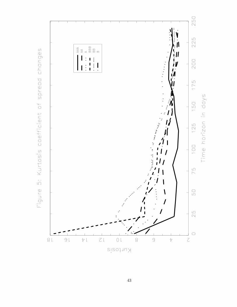
Figures 4 and 5 present estimates of skewness and kurtosis coefficients for the 5-year

(18)Given that spreads are first-difference stationary (see Section 3.3) standard results from time seriesanalysis, eg chapter 6 of Fuller (1996), imply the validity of a version of the Central Limit Theorem forSn+k − Sn under appropriate moment conditions on the innovations.

22

maturity spread changes for different ratings categories, plotted against length of

investment horizon.(19) The issue here is the degree to which the distributions of spread

changes appear to converge to normal distributions. An indication of this is the extent to

which kurtosis approaches three and skewness converges to zero. Figure 5 suggests that

the very high kurtosis evident in spread changes over short periods substantially dies off

as the period lengthens. For spread changes over 1 year, the kurtosis of spread changes for

all six ratings categories that we consider is close to or just over 3, the value kurtosis takes

for a normally distributed random variable. On the other hand, the skewness coefficients

for spread changes appear to turn from positive to negative as the length of the period

increases.

Using Monte Carlos, we calculated 95% confidence intervals for skewness and kurtosis

estimates for a 1-year horizon with overlapping observations assuming that the true

process was a random walk with drift and based on the same number of observations as in

our sample. For kurtosis, the confidence interval was 2.45 to 5.16, while for skewness it

was -1.40 to 1.40. This suggests that the estimated kurtosis and skewness for a 1-year

horizon were within reasonable sampling errors of the levels appropriate for normally

distributed processes.

4 Risk measures

4.1 Distributional assumptions

The results of the previous section imply it is reasonable to suppose that the distribution

of spreads over a 1-year horizon, Sjt for j = 1, 2, . . . , N − 1, is approximately joint normal

with variances and covariances based on our small-sample-adjusted estimates. We assume

that the distribution of the ‘spread’ in the default state, SNt ≡ − log(ξt)/k, is such that

the recovery rate, ξt, is beta distributed. This is consistent with the assumption of JP

Morgan (1997). We select the parameters of the beta distribution for ξt so that recoveries

have a mean and standard deviation of 51.13% and 25.45%. These were the moments

estimated by Carty and Lieberman (1996) in their study of recoveries on Moody’s rated

(19)The skewness and kurtosis plots are adjusted for small-sample bias using Monte Carlos.

23

defaulting senior unsecured bonds.(20) Finally, we suppose that recovery-rate risk is

independent across individual exposures and independent of other sources of risk. This is

the standard approach in credit risk modelling although it might be questioned.(21)

We experimented with different transition matrices. The baseline matrix we employed was

the transition matrix for US industrials estimated by Nickell, Perraudin and Varotto

(2000) using senior, unsecured ratings for all Moody’s-rated obligors from January 1970 to

December 1997, see Table C. This matrix is consistent with those reported in Carty and

Fons (1993) and Carty (1997) except for our use of more up-to-date data and the

restriction to industrials.(22) It made sense to employ transition matrices for industrials

since the Bloomberg spread data we employed was for that sector.(23)

Rather than employing a transition matrix based simply on the historical experience of

ratings transitions, Creditmetrics recommend that one use matrices for which the

long-run behaviour accords with the long-run, steady-state distribution of ratings. The

lower part of Table C contains a matrix of this type in which transition probabilities have

been adjusted to fit a given set of steady-state probabilities recommended by the

Creditmetrics manual. The Creditmetrics matrix differs significantly from our baseline

transition matrix estimated from Moody’s data. It implies higher volatility especially for

lower-rated obligors and has small probabilities of very large rating category changes for

highly-rated bond issuers.

4.2 Single rating grade VaRs

In Table D, we report single rating grade, 1-year holding-period VaRs for portfolios of 500

exposures, each having the same initial rating. Each exposure in the portfolio consists of a

5-year maturity,(24) pure discount bond so its price has the form exp[−Sjt(k)k] multiplied

(20)Carey (1998) provides some evidence that recoveries on private placements is higher at about 60%.(21)In a credit-derivative pricing model, Das and Tufano (1996) suppose that interest-rate andrecovery-rate risk are correlated.(22)It is also very similar to the one based on Moody’s data, which appears in Chapter 6 of theCreditmetrics manual.(23)We do not address the issue within this study of the stability of ratings transition matrices, either inthe time series dimension looked at by Blume, Lim and MacKinlay (1998) or the cross-sectional stabilitystudied by Nickell, Perraudin and Varotto (2000).(24)When we calculate a VaR for say an n-year maturity bond, we mean that the bond will have amaturity of n years at the end of the 1-year horizon of the VaR calculation.

24

by the price of a default-free pure discount bond.(25) We are only interested in the credit

risk component of total risk, so we only consider changes in the spread factor

exp[−Sjt(k)k] in our VaR calculation.

The baseline transition matrix employed in the VaR calculations is the matrix for US

industrials estimated by Nickell, Perraudin and Varotto (2000). This matrix differs from

those reported by Moody’s themselves in, for example, Carty (1997), only because of

differences in sample period. We report VaRs for 1% and 0.3% confidence levels. Many

banks use confidence levels like 0.3% (or even smaller) but 1% VaR calculations are more

statistically reliable since only 30 years of data are used in the estimation of ratings

transition matrices.

We also calculate VaRs using a transition matrix suggested by the Creditmetrics manual

which is designed to capture the steady-state behaviour of ratings changes (ie the

distribution of ratings changes over long horizons). This matrix has larger probabilities of

substantial ratings changes (including transitions into default) for highly-rated

exposures.(26) Throughout, we suppose that the correlation coefficient for the

credit-quality latent variables, ρ, equals 0.2.

We calculate VaRs in three ways: (i) default-mode (labelled ‘D’), (ii) mark-to-market

mode allowing for ratings transition and recovery-rate risk (labeled ‘D+T’), and (iii)

mark-to-market mode allowing for ratings transition, recovery rate and spread risk

(labelled ‘D+T+S’). Default-mode VaRs (D) effectively only count losses in value

associated with exposures that actually default. Mark-to-market mode calculations

(D+T) correspond to standard implementations of Creditmetrics.(27) In all cases, the

VaRs are scaled by the initial value of the portfolio and multiplied by 100. This scaling

means that they are of the same order as standard percentage capital charges like those

(25)We choose a 5-year maturity since this is the (value-weighted) average maturity for one bank withwhich we have had discussions. The effective maturity of a credit may be longer than thecontractually-specified one, since banks are often reluctant to raise their lending rates when a particularcustomer’s credit standing deteriorates for fear of spoiling a long-term banking relationship. Hence, 5years may be a reasonable assumption even when the average maturity of a bank’s book is shorter.(26)In the Moody’s data employed by Nickell, Perraudin and Varotto (2000) which comprised allnon-municipals rated by Moody’s in the period January 1970 to December 1997, not a single obligor ratedA or above defaulted within a one-year horizon; but the Creditmetrics transition matrix includes asignificant default probability even for AAA-rated borrowers.(27)When we omit spread risk, we set spreads equal to the sample averages of the Bloomberg data.

25

suggested by Basel Committee on Banking Supervision (1999).

As expected, the single rating grade VaRs reported in Table D increase sharply as credit

quality declines from AAA to CCC. The rate of increase is greatest for the default-mode

VaRs (D) and least for the mark-to-market VaRs with spread risk (D+T+S). In general,

D+T+S VaRs exceed those for D+T which in turn exceed those for D. The differences are

greatest for high credit quality exposures and largely disappear for CCC-rated exposures

since default risk dominates for low credit quality exposures.

The degree to which spread risk increases VaRs especially for high credit quality bonds is

striking. For AA and A-rated exposures, VaRs with spread risk are three times higher

when spread risk is included (and the calculation is performed using the Moody’s data

transition matrix). The increase is less considerable if the calculations employ the

Creditmetrics transition matrix because, for high-rated bonds, the transition risk is much

greater.

One may compare our results with those of Carey (2000). For single-grade portfolios

comprising BBB, BB, and B-rated exposures, his baseline 1% VaRs (equal to the

difference between the 99% loss percentile and the means in his Table C) equal 0.9%,

2.4% and 5.3%. These may be compared with our default-mode VaRs for BBB, BB and B

portfolios of 0.5%, 3.7%, and 8.6% respectively. The fact that our results are slightly

higher for BB and B (although not for BBB) probably reflects our more conservative

assumptions about loss given default.

An interesting issue is whether credit risk varies across industries. In particular, are

exposures to financials including banks more or less risky than those to industrials?(28)

The upper part of Table E contains VaRs for single rating grade portfolios calculated

using the ratings transition matrix for banks and other financials estimated by Nickell,

Perraudin and Varotto (2000).

For high credit quality portfolios, the bank-other-financial VaRs in the upper part of

Table E are very similar to the corresponding VaRs for industrials in Table D. When

(28)It is often presumed that banks of a given rating are less risky counterparties than industrials. This iswhy they receive favourable treatment in the Basel Accord and in the capital weight proposals in BaselCommittee on Banking Supervision (1999).

26

credit quality is low, however, the VaRs based on a bank and other financial transition

matrix are higher. This reflects the fact, noted by Nickell, Perraudin and Varotto (2000),

that when a bank’s credit standing declines below BBB, the likelihood that it will survive

is much smaller than for a comparably-rated industrial.

Another important issue is the sensitivity of our results to assumptions about recovery

rates. Carey (1998) argues that recoveries on private placements (which in some ways

resemble loans) is higher than those on bonds. The lower part of Table E reports VaRs

assuming a mean recovery rate of 60% rather than the 51% rate used in all our other VaR

calculations. The VaRs with the higher recovery rates are broadly unchanged from those

reported in Table D for investment quality (BBB and above) ratings categories. For very

low quality credits, the VaRs with the higher recovery rate are about a third lower in the

B and CCC categories.

Lastly, it is important to consider the sensitivity of our calculations to the degree of

diversification. Table F contains 0.3% VaRs for single rating grade portfolios satisfying

our baseline assumptions (five-year maturity, industrial transition matrix, spread and

transition risks included), but containing 5, 10, 50, and 100 equal-sized exposures rather

than the 500 exposures assumed in the VaRs of Tables D and E. The most striking feature

of the results in Table F is that, in the case of low credit quality portfolios, the VaRs only

become substantially larger than those in Table D when the number of exposures drops to

50 or below. This suggests that diversification begins to influence VaR calculations rather

early as the number of exposures in the portfolio increases. In part, this reflects the fact

that spread risk, which dominates for high credit quality exposures, is highly correlated.

4.3 Value at Risk for actual bank portfolios

Single rating grade VaRs reveal much about the structure of credit risk, but it is also

important to consider portfolios like those of actual banks made up of differently-rated

exposures. Table G reports 1% and 0.3% VaRs for three such realistic portfolios under

different assumptions about the correlation between the latent variables that generate

ratings transitions for different obligors. The ratings distributions of the three portfolios

(each of which contains 500 equal-sized exposures) are based on data in Gordy (2000).

27

The ‘average quality portfolio’ has the same ratings distribution as the average of a large

sample of US banks surveyed by the Federal Reserve Board (see Gordy (2000)). The

‘high-quality’ portfolio has the average distribution of a subset of banks surveyed which

had relatively low-risk portfolios. The ‘investment quality’ portfolio has the same shares

invested in different ratings categories as that part of the average portfolio which was

rated BBB or above.(29)

We calculate VaRs under different assumptions about the correlation coefficient of the

latent variables, denoted ρ, namely that ρ equals 0.1, 0.2, or 0.3. The Creditmetrics

manual reports a matrix of typical correlation coefficients for a sample of bonds. The

average of the off-diagonal entries in their correlation matrix is 0.198, to some extent

justifying our choice of 0.2 as a baseline value.

The portfolio VaRs in Table G again suggest that spread risk is important, especially

when the correlation parameter ρ is relatively small. In this case, transition risk is

diversified away in large portfolios but spread risk is correlated across different exposures

and hence is not diversified. Even when ρ = 0.2, the high-quality portfolio has a VaR

which is a third higher when spread risk is included.

For the average quality portfolio, the VaRs are about a fifth higher with spread risk for ρ

= 0.2 and a third higher for ρ = 0.1. These and other results appear less sensitive to the

choice of transition matrix when one calculates portfolio VaRs rather than VaRs for

individual bond values. It is noticeable that, with the baseline correlation coefficient of ρ

= 0.2, the average portfolio VaR (for our assumed confidence levels) is between 5.5% and

7%, only a little lower than the 8% level built into the 1988 Basel Accord. Using the

Creditmetrics transition matrix, the figures are slightly higher at 6% to 7.5%.

Again, one may compare the default-mode VaRs reported in Table G with the results of

Carey (2000) since he calculates quantiles of the loss distribution for the same average

quality portfolio. The 1% VaR implied by the results in his Table 2 is 2.1%. Once again,

(29)More specifically, the average portfolio contains 15 AAA, 25 AA, 67 A, 156 BBB, 162 BB, 56 B, and20 CCC-rated credits each of the same face value and the same maturity of 5 years. The high-qualityportfolio which is another portfolio considered by Gordy (2000) contains 19 AAA, 30 AA, 146 A, 190BBB, 95 BB, 13 B, and 6 CCC-rated credits. The investment quality portfolio contains 28 AAA, 48 AA,128 A, 297 BBB-rated credits.

28

this is probably slightly lower than our baseline (ρ = 0.2) default-mode VaR for the

average portfolio of 3.2% because of our more conservative loss given default assumptions.

4.4 The effects of maturity

A dimension of credit risk that one might expect would be important is maturity. Table H

shows 0.3% VaRs calculated on a default-mode basis (D) and on a mark-to-market basis

with and without spread risk (D+T+S and D+T, respectively) for our three portfolios

and for different maturities. The holding period for the VaR in all cases is 1 year and the

maturities of the portfolios at the end of that year are 2, 5 and 10 years.

At short maturities spread risk matters very little, reflecting the fact that spreads are

multiplied by maturity when they enter bond pricing formulae. On the other hand,

recovery rates are independent of maturity, so these come to matter substantially as

maturity shrinks. These observations also explain why high-quality debt shows a much

more marked dependence on maturity than the average portfolio which contains a

substantial proportion of non investment grade exposures.

4.5 Sensitivity analysis

Given the multi-stage nature of the estimations and calculations we perform in this paper,

it is difficult to put standard errors on the VaRs we report. (To do so would involve

repeated simulation of computationally demanding Monte Carlo estimates.) In Table I,

we therefore perform a sensitivity analysis, perturbing the estimates employed in our

calculations by reasonable amounts and then seeing how this affects VaRs. We are

particularly interested in the robustness of our finding that spread risk is important

especially for high credit quality portfolios. Hence, in Table I, we report portfolio VaRs

under the assumption that all the spread volatilities and covariances are reduced by one

standard deviation. The 1% VaR for the average portfolio falls from 5.6% to 5.1% while

that for the investment quality portfolio drops from 2.8% to 2.2%. We conclude from this

that our results are reasonably robust to changes in the spread volatility estimates.

29

5 Conclusion

This paper attempts to quantify the riskiness of different kinds of credit exposure, looking

both at credit quality and maturity dimensions. We also examine the composition of

credit risk, in particular the relative importance of risks associated with ratings

transitions, recovery rates and changes in spreads for different ratings categories.

Our conclusions are, first, that spread risk is important for relatively high-quality debt,

and models such as Creditmetrics that assume zero spread risk may underestimate the

riskiness of highly-rated portfolios.

Second, under reasonable assumptions about correlations of ratings transitions, the total

VaRs we obtain including spread risk are of the order of 7% for a portfolio of 5-year

maturity exposures with a credit quality distribution equal to the average of a large

sample of US banks. It is interesting that this is close to the 8% required by the 1988

Basel Accord. Similar investment quality portfolios, on the other hand, yield VaRs of the

order of 3%-4%.

Third, the dependence of VaRs on maturity depends very much on whether the exposures

are low or high credit quality. Low credit quality exposures are quite insensitive to

maturity because recovery risk is a substantial fraction of total risk. For high credit

quality exposures, spread risk is more important and this leads to a strong positive

dependence on maturity since spreads are scaled up by maturity when they enter bond

values expressions.

An important question is to what degree are our conclusions applicable to bank loan

books as well as to bond portfolios?(30) Typically, banks adjust their lending rates quite

infrequently so some of our conclusions about the importance of spread risk might appear

to be less relevant for loan portfolios. Furthermore, the impact of fluctuations in value

due to liquidity shocks might affect bond portfolios differently from portfolios of loans.

In our view, the smoothness of loan spreads reflects the fact that banks are conducting

long-term relationships with borrowers and not any corresponding smoothness in the

(30)Carey (1995) considers the consistency of bond and loan pricing while Altman and Suggitt (2000)compare the transition probabilities of loans and bonds.

30

credit standing of borrowers. Furthermore, our procedures for estimating spread risk over

long horizons specifically filters out high-frequency, mean-reverting components of risk

such as liquidity shocks. It is plausible, therefore, to argue that a reasonable fraction of

the spread risk we measure is applicable to loan as well as bond portfolios.

31

Table A: Descriptive statistics for daily spread data

Means VolatilitiesMaturity (years) 2 5 10 2 5 10AAA 27.7 31.2 30.7 2.3 2.1 2.8

(0.2) (0.1) (0.2) (0.1) (0.1) (0.3)AA 34.8 35.2 36.3 2.5 2.1 2.8

(0.2) (0.1) (0.2) (0.0) (0.1) (0.3)A 46.4 54.1 58.7 2.3 2.2 2.8

(0.4) (0.3) (0.3) (0.2) (0.1) (0.3)BBB 70.1 74.4 80.5 2.1 2.1 2.8

(0.7) (0.5) (0.4) (0.1) (0.1) (0.3)BB 163.1 179.6 216.9 3.1 3.0 3.8

(1.9) (1.1) (0.9) (0.2) (0.2) (0.4)B 307.0 334.5 350.9 3.8 4.0 4.3

(2.2) (1.5) (1.1) (0.3) (0.3) (0.4)Note: Means are sample means of spread levels in basispoints. Volatilities are sample standard deviations of dailyspread changes in basis points. Newey-West standarderrors appear in parentheses.

Table B: Five-year spread correlations at a one-year horizon

VolatilitiesAAA AA A BBB BB B0.41 0.45 0.95 1.27 2.42 4.77

(0.09) (0.10) (0.21) (0.27) (0.53) (1.05)Correlation matrix

AAA AA A BBB BB BAAA 1.00 0.75 0.63 0.67 0.51 0.53AA 0.75 1.00 0.76 0.73 0.49 0.57A 0.63 0.76 1.00 0.91 0.62 0.59BBB 0.67 0.73 0.91 1.00 0.71 0.57BB 0.51 0.49 0.62 0.71 1.00 0.62B 0.53 0.57 0.59 0.57 0.62 1.00Note: Asymptotic standard errors appear in brackets.Volatilities are standard deviations of one-year changesin spreads multiplied by maturity (5) and by 100.

32

Table C: Transition matrices

Moody’s data †AAA AA A BBB BB B CCC D

AAA 91.60 7.80 0.70 0.00 0.00 0.00 0.00 0.00AA 1.10 89.30 9.10 0.30 0.20 0.00 0.00 0.00A 0.10 1.90 92.40 4.80 0.60 0.20 0.00 0.00BBB 0.00 0.10 3.90 89.90 4.90 0.80 0.10 0.20BB 0.00 0.10 0.40 3.40 87.00 7.40 0.20 1.50B 0.00 0.10 0.20 0.50 6.20 84.00 2.30 6.80CCC 0.00 0.00 0.00 0.60 1.90 7.30 73.10 17.00D 0.00 0.00 0.00 0.00 0.00 0.00 0.00 100.00

Creditmetrics ‡AAA AA A BBB BB B CCC D

AAA 87.74 10.93 0.45 0.63 0.12 0.10 0.02 0.02AA 0.84 88.23 7.47 2.16 1.11 0.13 0.05 0.02A 0.27 1.59 89.05 7.40 1.48 0.13 0.06 0.03BBB 1.84 1.89 5.00 84.21 6.51 0.32 0.16 0.07BB 0.08 2.91 3.29 5.53 74.68 8.05 4.14 1.32B 0.21 0.36 9.25 8.29 2.31 63.89 10.13 5.58CCC 0.06 0.25 1.85 2.06 12.34 24.86 39.97 18.60D 0.00 0.00 0.00 0.00 0.00 0.00 0.00 100.00Note: Transition matrices (in per cent) are for one year.† Source: Nickell, Perraudin and Varotto (2000).‡ Source: JP Morgan (1997).

33

Table D: Single grade VaRs

Using Moody’s data transition matrix(Nickell, Perraudin and Varotto (2000))

1% VaR 0.3% VaRRating D+T+S D+T D D+T+S D+T DAAA 0.95 0.10 0.00 1.13 0.16 0.00AA 1.20 0.40 0.00 1.52 0.57 0.00A 2.31 0.67 0.00 2.74 1.03 0.00BBB 3.65 2.42 0.95 4.68 3.54 1.69BB 7.43 5.80 4.12 9.40 7.72 5.88B 13.11 10.67 9.77 15.76 13.58 13.80CCC 17.00 15.50 15.00 19.87 18.23 18.22

Using JP Morgan transition matrix(JP Morgan (1997))

1% VaR 0.3% VaRRating D+T+S D+T D D+T+S D+T DAAA 1.04 0.54 0.19 1.31 0.86 0.33AA 1.58 1.09 0.18 2.16 1.58 0.33A 2.47 1.12 0.26 3.03 1.66 0.45BBB 3.46 2.01 0.45 4.30 2.81 0.79BB 8.56 6.58 3.70 10.88 8.85 5.54B 14.14 11.67 8.58 17.10 14.80 11.50CCC 18.85 17.68 15.55 22.15 21.26 19.05Notes: Portfolios consist of 500 exposures of equal face value.VaRs are measured in per cent of the expected value. The correlationcoefficient of the latent transitions, ρ, equals 0.2.D indicates default-mode VaR calculation.D+T corresponds to standard Creditmetrics.D+T+S corresponds to Creditmetrics including spread risk.

34

Table E: Single grade VaRs

Using bank transition matrix(Nickell, Perraudin and Varotto (2000))

1% VaR 0.3% VaRRating D+T+S D+T D D+T+S D+T DAAA 0.94 0.10 0.00 1.12 0.13 0.00AA 1.24 0.33 0.00 1.50 0.43 0.00A 2.29 0.74 0.00 2.76 1.08 0.00BBB 3.68 2.21 0.99 4.61 2.95 1.61BB 9.25 8.08 4.19 11.90 10.83 5.86B 12.21 9.02 9.85 14.72 11.52 12.95CCC 21.88 21.81 17.51 24.05 24.01 20.53

Using industrial transition matrix 60% recovery rate(JP Morgan (1997))

1% VaR 0.3% VaRRating D+T+S D+T D D+T+S D+T DAAA 0.95 0.10 0.00 1.13 0.15 0.00AA 1.24 0.41 0.00 1.50 0.59 0.00A 2.27 0.68 0.00 2.72 0.98 0.00BBB 3.57 2.18 0.76 4.52 3.23 1.28BB 6.92 4.89 3.25 8.68 6.66 4.78B 11.58 7.97 7.07 13.58 10.29 9.62CCC 13.42 11.25 10.56 15.50 13.59 13.20See notes to Table D.

Table F: Diversification: 1% VaRs

Using Moody’s data transition matrix(Nickell, Perraudin and Varotto (2000))

Rating # Bonds100.00 50.00 10.00 5.00

AAA 1.11 1.06 1.13 1.15AA 1.46 1.53 1.67 2.08A 2.86 2.82 3.15 3.80BBB 4.91 5.15 8.88 13.38BB 10.10 10.69 15.72 21.12B 16.73 17.84 24.68 33.99CCC 21.70 22.75 32.88 42.74See notes to Table D.

35

Table G: Portfolio VARs

Using industrial transition matrix(Nickell, Perraudin and Varotto (2000))

1% VaR 0.3% VaRPortfolio ρ D+T+S D+T D D+T+S D+T DAverage 0.10 4.69 2.69 1.95 5.65 3.51 2.68

0.20 5.58 4.26 3.18 7.05 5.90 4.550.30 6.76 5.80 4.33 9.05 8.47 6.25

High 0.10 3.31 1.63 1.03 3.98 2.20 1.370.20 3.76 2.63 1.52 4.76 3.60 2.330.30 4.41 3.58 2.11 6.10 5.33 3.13

Investment 0.10 2.55 1.01 0.41 3.04 1.43 0.600.20 2.84 1.65 0.60 3.56 2.48 0.970.30 3.17 2.27 0.81 4.31 3.49 1.51

Using Creditmetrics transition matrix(JP Morgan (1997))

1% VaR 0.3% VaRPortfolio ρ D+T+S D+T D D+T+S D+T DAverage 0.10 4.98 3.14 1.79 6.03 4.07 2.36

0.20 6.03 4.74 2.85 7.62 6.41 4.060.30 7.27 6.29 3.89 9.66 8.86 5.51

High 0.10 3.42 1.82 0.87 4.13 2.36 1.180.20 4.01 2.87 1.33 5.08 3.88 1.950.30 4.70 3.74 1.81 6.27 5.32 2.85

Investment 0.10 2.60 0.98 0.27 3.14 1.32 0.400.20 2.80 1.61 0.36 3.50 2.34 0.620.30 3.19 2.19 0.43 4.22 3.15 0.87

Notes: Portfolios consist of 500 exposures of equal face value.The ratings compositions of portfolios is given in the text.VaRs are measured in per cent of the expected value.D indicates default-mode VaR calculation.D+T corresponds to standard Creditmetrics.D+T+S corresponds to Creditmetrics including spread risk.

Table H: Effect of maturity on 0.3% VaRs

2yr bonds 5yr bonds 10yr bondsPortfolio D+T+S D+T D+T+S D+T D+T+S D+TAverage quality 5.97 5.83 7.05 5.90 11.62 6.43High quality 3.18 2.94 4.76 3.60 8.79 4.73Investment quality 1.79 1.49 3.56 2.48 7.06 4.00See notes to Table D. ρ = 0.2.

36

Table I: Sensitivity analysis 1% VaR

Using Moody’s data transition matrix(Nickell, Perraudin and Varotto (2000))

Portfolio D+T+S D+T DAverage 5.08 4.26 3.18High 3.18 2.63 1.52Investment quality 2.24 1.65 0.60Notes: Calculations are same as in Table G except thatspread variances are reduced by one standard deviation.The composition of the portfolios is explained in the text.Simulations use transition matrix based on Moody’s data andρ = 0.2. For definitions of D, D+Tand D+T+S, see notes to Table D.

37

Notes to Figures

Figure 1The figure shows conditional volatilities for different horizons estimated on daily spread dataassuming they follow (i) an Onstein-Uhlenbeck, (ii) an arithmetic Brownian motion with drift, and(iii) a discrete-time, first-difference stationary process. Maximum Likelihood estimation isemployed in cases (i) and (ii) while in case (iii) the volatilities are estimated using anon-parametric technique described in the text.

Figure 2Volatilities for different ratings are plotted against maturity for four different investment horizons.Volatilities are divided by the square root of the investment horizon and multiplied by 100 so theyare in per cent. For the one-day horizon, investment grade volatilities (BBB2 and above) showalmost no variation for a given maturity. Spreads for longer horizons vary substantially acrossratings category for given maturities.

Figure 3The ratio of estimated spread variances for different investment horizons (k) to k times the one-dayvariance is shown plotted against k. For a random walk, the (population) ratio equals unity. Forfirst difference stationary series, the ratio converges asymtotically to a constant for large k.

Figure 4The skewness coefficient (defined as the third central moment divided by the cubed standarddeviation) is shown for spread changes over different time horizons and ratings categories.

Figure 5The kurtosis coefficient (defined as the fourth central moment divided by the squared variance) isshown for spread changes over different time horizons and ratings categories.

38

39

40

41

42

43

Appendix

Cochrane-type bias correction

We assume that the data generating process is a pure unit root process, ie equation (7) becomes

Si − Si−1 = µ+ εi (A1)

with εi assumed to be i.i.d. with expectation zero and variance σ2ε . We are interested in

constructing an estimator for σ2ε using k-lagged differences, ie

Sn − Sn−k = kµ+k−1∑j=0

εn−j

Using k(ST − S0)/T as an estimator for µ we can write the nominator of the standard samplevariance

Nσ =T∑

n=k

((Sn − Sn−k)− k

T(ST − S0)

)2

=T∑

n=k

kµ+

k−1∑j=0

εn−j − k

T

Tµ+

T−1∑j=0

εT−j

2

=T∑

n=k

n∑

j=n−k+1

εj − k

T

T∑j=1

εj

2

Defining Zn =∑n

j=n−k+1 εj and using the fact that the εi are i.i.d with zero mean (ieVar(ε) = E(ε2)) we get

E(Nσ) =T∑

n=k

(E(Z2

n)−2kTE(ZnZT ) +

k2

T 2E(Z2

T ))

= E(ε2)T∑

n=k

(k − 2k2

T+

k2

T

)= σ2

ε (T − k + 1)(T − k)k

T

So in order to get an unbiased estimator for σ2ε using the quantity Nσ we have to multiply it by

T

k(T − k + 1)(T − k)

which is just the Cochrane adjustment. So we define

σ2(k) =T

(T − k)(T − k + 1)

T∑j=k

[(Sj − Sj−k)− k

T(ST − S0)

]2

(A2)

as the Cochrane estimator of the variance.

We can repeat the above procedure to obtain unbiased versions for the estimation of thecorrelation between categories, the skewness and the kurtosis.

For estimation of the correlation we assume that the covariance structure between categories isgiven by

Cov(εAj , εB

i ) = E(εAj , εB

i ) = δijρ

44

where δij = 1 for i = j and zero elsewhere. An unbiased estimator of the sample covarianceγAB(k) in the random walk model is then (proceeding as above)

γAB(k) =T

(T − k)(T − k + 1)

T∑j=k

[(SAj − SA

j−k)− µA][(SBj − SB

j−k)− µB ] (A3)

(use the Cochrane sample means µ = kT (ST − S0)). The correlations ρAB(k) can then be estimated

as

ρAB(k) =γAB(k)

σ(k)Aσ(k)B(A4)

The sample skewness estimator is a quotient with nominator

NS =T∑

n=k+1

((Sn − Sn−k)− k

T(ST − S0)

)3

With the technique above we get

E(NS) = (T − k + 1)(T − k)(T − 2k)k

T 2E(ε3)

So the adjusted skewness estimator is given by

T 2

(T − k + 1)(T − k)(T − 2k)NS

(σ(k))3

Finally, for the sample kurtosis estimator the nominator is

NK =T∑

n=k+1

((Sn − Sn−k)− k

T(ST − S0)

)4

andE(NK) = (T − k + 1)(T − k)(T 2 − 3kT + 3k2)

k

T 3E(ε4)

So the adjusted kurtosis estimator is given by

T 3

(T − k + 1)(T − k)(T 2 − 3kT + 3k2)NK

(σ(k))4

45

References

Altman, E I (1997), ‘Rating migration of corporate bonds - comparative results andinvestor/lender implications’, mimeo, Salomon Brothers, New York.

Altman, E I and Kao, D L (1992a), ‘The implications of corporate bond ratings drift’,Financial Analysts Journal, pages 64-75.

Altman, E I and Kao, D L (1992b), ‘Rating drift of high yield bonds’, Journal of FixedIncome, pages 15-20.

Altman, E I and Suggitt, H J (2000), ‘Default rates in the syndicated bank loan market: amortality analysis’, Journal of Banking and Finance, Vol.24(1-2), pages 229-54.

Anderson, T W (1971), The statistical analysis of time series, Wiley, New York.

Basel Committee on Banking Supervision (1999), ‘Consultative paper on a new capitaladequacy framework’, Bank for International Settlements, Basel, Switzerland.

Beveridge, S and Nelson, C R (1981), ‘A new approach to decomposition of economic timeseries into permanent and transitory components with particular attention to measurement of thebusiness cycle’, Journal of Monetary Economics, Vol.7, pages 151-74.

Blume, M E, Lim, F and MacKinlay, A C (1998), ‘The declining credit quality of UScorporate debt: myth or reality?’, Journal of Finance, Vol.53(4), pages 1,389-413.

Carey, M (1995), ‘Are bank loans mispriced?’, unpublished mimeo, Federal Reserve Board,Washington DC.

Carey, M (1998), ‘Credit risk in private debt portfolios’, Journal of Finance, Vol.53(4), pages1,363-87.

Carey, M (2000), ‘Dimensions of credit risk and their relationship to economic capital’, mimeo,Federal Reserve Board, Washington DC.

Carty, L V (1997), ‘Moody’s rating migration and credit quality correlation, 1920-1996’, Specialcomment, Moody’s Investors Service, New York.

Carty, L V and Fons, J (1993), ‘Measuring changes in credit quality’, Moody’s Special Report,Moody’s Investors Service, New York.

Carty, L V and Lieberman, D (1996), ‘Corporate bond defaults and default rates’, InvestorsReport Service, Moody’s Global Credit Research.

Cochrane, J H (1988), ‘How big is the random walk in GNP?’, Journal of Political Economy,Vol.96(5), pages 893-920.

Collin-Dufresne, P, Goldstein, R S and Martin, J S (1999), ‘The determinants of creditspread changes’, mimeo, Ohio State University, Columbus, OH.

Crouhy, M, Galai, D and Mark, R (1999), ‘A comparative analysis of current credit riskmodels’, Journal of Banking and Finance, Vol.24(1-2), pages 59-118.

Das, S and Tufano, P (1996), ‘Pricing credit sensitive debt when interest rates, credit ratingsand credit spreads are stochastic’, Journal of Financial Engineering, Vol.5, pages 161-98.

Duffee, G R (1998), ‘The relation between Treasury yields and corporate bond yield spreads’,

46

Journal of Finance, Vol.53(6) pages 2,225-41.

Duffee, G R (1999), ‘Estimating the price of default risk’, Review of Financial Studies,Vol.12(1), pages 197-226.

Fuller, W (1996), Introduction to statistical time series, Springer-Verlag, New York.

Gordy, M (1999), ‘A comparative anatomy of credit risk models’, Journal of Banking andFinance, Vol.24(1-2), pages 119-50.

Greenspan, A (1998), ‘The role of capital in optimal banking supervision and regulations’,FRBNY Economic Policy Review, pages 163-68.

Jones, E P, Mason, S P and Rosenfeld, E (1984), ‘Contingent claims analysis of corporatecapital structures: an empirical investigation’, Journal of Finance, Vol.39(3), pages 611-27.

JP Morgan (1997), Creditmetrics - technical document, JP Morgan, New York.

Kwiatkowski, D, Phillips, P, Schmidt, P and Shin, Y (1992), ‘Testing the null hypothesisof stationary against the alternative of a unit root’, Journal of Econometrics, Vol.54, pages 159-78.

Litterman, R and Iben, T (1991), ‘Corporate bond valuation and the term structure of creditspreads’, Journal of Portfolio Management, pages 52-64.

Lo, A W (1991), ‘Long-term memory in stock market prices’, Econometrica, Vol.59(a), pages1,279-313.

Lopez, J A and Saidenberg, M R (1999), ‘Evaluating credit risk models’, Journal of Bankingand Finance, Vol.24(1-2), pages 151-66.

Lucas, D J and Lonski, J G (1992), ‘Changes in corporate credit quality 1970-1990’, Journalof Fixed Income, pages 7-14.

Merton, R C (1974), ‘On the pricing of corporate debt: the risk structure of interest rates’,Journal of Finance, Vol.29, pages 449-70.

Morris, C, Neal, R and Rolph, D (1999), ‘Credit spreads and interest rates’, mimeo, IndianaUniversity, Indianapolis.

Nickell, P, Perraudin, W R and Varotto, S (1998), ‘Ratings versus equity based credit riskmodels: an empirical study’, forthcoming Bank of England working paper.

Nickell, P, Perraudin, W R and Varotto, S (2000), ‘The stability of ratings transitions’,Journal of Banking and Finance, Vol.24(1-2), pages 203-28.

Pedrosa, M and Roll, R (1998), ‘Systematic risk in corporate bond credit spreads’, Journal ofFixed Income, pages 7-26.

Pitts, C and Selby M (1983), ‘The pricing of corporate debt: a further note’, Journal ofFinance, Vol.8, pages 1,311-13.

Sarig, O and Warga, A (1989), ‘Some empirical estimates of the risk structure of interestrates’, Journal of Finance, Vol.44(5), pages 1351-60.

Standard and Poor’s (1998), ‘Ratings performance 1997 - stability and transition’, ResearchReport, Standard and Poor’s, New York.

47